DISCUSSION PAPER SERIES

IZA DP No. 11433

Christian BelzilFrançois Poinas

Estimating a Model of Qualitative and Quantitative Education Choices in France

MARCH 2018

Any opinions expressed in this paper are those of the author(s) and not those of IZA. Research published in this series may include views on policy, but IZA takes no institutional policy positions. The IZA research network is committed to the IZA Guiding Principles of Research Integrity.The IZA Institute of Labor Economics is an independent economic research institute that conducts research in labor economics and offers evidence-based policy advice on labor market issues. Supported by the Deutsche Post Foundation, IZA runs the world’s largest network of economists, whose research aims to provide answers to the global labor market challenges of our time. Our key objective is to build bridges between academic research, policymakers and society.IZA Discussion Papers often represent preliminary work and are circulated to encourage discussion. Citation of such a paper should account for its provisional character. A revised version may be available directly from the author.

Schaumburg-Lippe-Straße 5–953113 Bonn, Germany

Phone: +49-228-3894-0Email: publications@iza.org www.iza.org

IZA – Institute of Labor Economics

DISCUSSION PAPER SERIES

IZA DP No. 11433

Estimating a Model of Qualitative and Quantitative Education Choices in France

MARCH 2018

Christian BelzilCREST, CNRS, Ecole Polytechnique, CIRANO and IZA

François PoinasToulouse School of Economics, University of Toulouse Capitole

ABSTRACT

IZA DP No. 11433 MARCH 2018

Estimating a Model of Qualitative and Quantitative Education Choices in France*

We estimate a structural model of education choices in which individuals choose between

a professional (or technical) and a general track at both high school and university levels

using French panel data (Génération 98). The average per-period utility of attending

general high school (about 10,000 euros per year) is 20% higher than that of professional

high school (about 8000 euros per year). About 64% of total higher education enrollments

are explained by this differential. At the same time, professional high school graduates

would earn 5% to 6% more than general high school graduates if they both entered

the labor market around age 18. The return to post-high school general education is

highly convex (as in the US) and is reaped mostly toward the end of the higher education

curriculum. Public policies targeting an increase in professional high school enrollments of

10 percentage points would require a subsidy of 300 euros per year of professional high

school.

JEL Classification: C51, I23, I26, J24

Keywords: education choices, returns to schooling, professional education, structural model

Corresponding author:Christian BelzilDepartment of EconomicsEcole Polytechnique91128 Palaiseau CedexFrance

E-mail: christian.belzil@polytechnique.edu

* A previous version of this paper has been circulated under the title “A Qualitative Approach to the Estimation

of the Returns to Schooling in France”. We are grateful to participants to the Association Française de Sciences

Economiques congress 2014 in Lyon, European Economic Association congress 2014 in Toulouse, International

Association for Applied Econometrics conference 2016 in Milan, and seminar participants at BETA - University of

Nancy in 2017, CREST-INSEE Paris in 2017 and LMU Munich in 2017.

1 Introduction

We estimate a structural model of education choices which captures both thequalitative and quantitative dimensions of education choices using French paneldata (Generation 98 ) on educational choice trajectories made in the 1990’s andearly career wages between 1998 and 2003. One specificity of the French systemis the existence of a professional track at the senior high school level (lycee)and a technical track (BTS 1 and DUT 2) at the university level. These tracksdiffer from the general track in the type of training delivered to the students.The professional track provides training to acquire professional skills specificto manual or clerical occupations (e.g. plumbing, butchery, logistics) and thetechnical track teaches students technical skills (e.g. in commerce and sales,agronomy, chemistry) to occupy technical support functions. All those whohave obtained a senior high school degree retain the option to enter general ortechnical higher education at a later stage. By modeling all of these aspects, wecan separately identify the professional-general and the technical-general wagedifferentials from their utility differentials and can also estimate the disutilityof switching tracks.

We use the model estimates to evaluate the cost of policies reducing thegeneral-professional net utility gap in order to increase professional high schoolenrollments. Our paper therefore contributes to the structural literature on ed-ucation choices, to the voluminous literature on estimating returns to schoolingand also to the public policy debate about the relative merits of general andprofessional education systems.3

The main findings are as follows. Our structural estimates reveal that theaverage utility of attending general high school (about 10,000 euros per year)is 20% higher than for professional high school. This differential may be inter-preted as an indication that general education entails a much higher consump-tion value than professional high school. At the same time, professional highschool graduates would earn 5% to 6% more than general high school graduatesif they both entered the labor market around age 18.

Individual heterogeneity in per-period utilities of attending education isfound to be important but its distribution appears to be more compressed thanwhat has been estimated for the US.4 About half of individual heterogeneity intastes for schooling is explained by parental background while the other half isexplained by persistent unobserved heterogeneity.

Our model provides an explanation for why very few individuals switch fromprofessional high school to general higher education as we find that the switchingcost of entering general education is about 1340 euros per year and therefore

1Brevet de Technicien Superieur2Diplome Universitaire de Technologie3In February 2018, the French government announced its intention to stimulate an increase

in apprenticeship enrollments (a subset of professional high school enrollments) with the in-troduction of a monthly subsidy of 30 euros paid directly to apprentices. See “Apprentissage,les grands axes de la reforme” (in French), http://www.lemonde.fr, 9 February 2018.

4Keane and Wolpin (1997) is the seminal piece in the literature. The structural literatureis surveyed in Belzil (2007).

2

represents a 20% reduction in the utility of attending general higher educationwhen compared with an individual graduating from a general high school.

As our model separates the qualitative dimension from the usual quanti-tative approach to the return to schooling, we can also assert that the returnto general education is highly convex (as in the US) and is reaped toward theend of the higher education curriculum. Indeed, the average return to generalhigher education is about 7% per year of education but the marginal return ispractically 0 during the first 2 years. The total wage premium of a completehigher education curriculum in the general track compared with a general highschool degree is about 34%.5

The convexity of the returns to higher education and the relatively highutility cost of switching from the professional to the general track imply thatthe option value of a general education track is much higher than that of aprofessional high school degree. The discounted utility gain of a high schoolprofessional education (measured until age 30) is found to be 7,715 euros whilethe option value of a professional high school degree is practically 0.

Finally, we find that an increase in the per-period utility of attending pro-fessional high school of 300 euros per year of attendance would be sufficient toraise enrollments by 10 percentage points (from 28% to 38%) and would alsoreduce high school drop-out by 3 percentage points (from 16% to 13%) andhigher education enrollments by 5 percentage points (from 44% to 39%).

Indeed, equalizing the net utilities of professional and general high schoolswould dramatically reduce the incentives to attend higher education. Our es-timates indicate that about 64% of total higher education enrollments are ex-plained by the existing general-professional utility differential at the high schoollevel. Without it, only 16% of the population would enroll in higher education(either general or technical). Interestingly, setting the utilities of technical andgeneral higher education to an equal level (while leaving the high school utilitydifferential unchanged) would reduce general higher education enrollments by 8percentage points. As a result, about 75% of all higher education enrollmentswould be in the technical track.

The remaining portion of the paper is structured as follows. In Section 2, wediscuss the related literature. In the following section, we describe the Frencheducational system in details. In Section 4, we present the data and the modelthat we estimate structurally is presented in Section 5. The next section isdevoted to the main results.

2 Background Literature

Our paper contributes to the literature on education choices. A first generationof structural microeconometric papers modeling education within a partial equi-

5While this estimate may seem much lower than most college-high school wage differentialreported for the late 90’s and early 2000’s in the US (usually between 70% and 80%), it isimportant to note that most estimates reported for the US are obtained ordinary least squaresand do not account for selectivity.

3

librium framework has focussed on issues such as occupation choices (Keane andWolpin, 1997), the decision to drop-out of high school (Eckstein and Wolpin,1999), evaluating the impact of borrowing constraints on education (Keane andWolpin, 2001) or measuring the ability bias in the presence of a convex wageschooling relationship (Belzil and Hansen, 2002). A relatively smaller number ofpapers have modeled schooling and occupational choices within an equilibriumframework. For instance, Heckman, Lochner, and Taber (1998) and Lee andWolpin (2010) estimated equilibrium models of the labor market using aggre-gate production technologies so to identify the major causes explaining changesin the wage distribution and in employment patterns. Gemici and Wiswall(2014) investigated movements in college major specific skill prices (especiallythe sciences) and document the importance of changes in schooling cost andgender specific changes in household production needed to explain changes inmajor choices. All of those papers, except for Gemici and Wiswall (2014), usethe 1979 cohort of the National Longitudinal Survey of Youth (the NLSY79)and naturally focus on the quantitative dimension of schooling. They thereforeignore the qualitative aspects.

A second contribution is the estimation of the qualitative aspects of thereturns to schooling. This dimension has been neglected in the empirical lit-erature. This may look surprising as in most western countries, educationaldecisions entail a qualitative dimension. In the US, the qualitative dimension isparticularly relevant in higher education when individuals select a college major.It is now widely recognized that the choice of a college major can have as muchimplications for future earnings than the decision to invest in post-secondaryeducation. For instance, many US studies have reported that the wage gapbetween science-engineering majors and humanities are virtually as high as thewage gap between college and high school graduates.6

Although the distinction between professional and general high school trackshas not attracted much attention in the US, some studies have attempted tomeasure the differences in returns between tracks. For instance, Altonji (1995)uses variation in the curriculum of high school programs across the US and findsa small positive effect of taking more academic subjects in high school.7 Meer(2007) estimates the impact of attending secondary vocational education onincome in the US. His findings are consistent with the presence of comparativeadvantage in the type of tracking chosen by high school students.

In continental Europe, qualitative educational choices are particularly im-portant as the general education system co-exists with an important professionaltrack. Indeed, the economic success of many countries is sometimes imputedto an efficient apprenticeship or vocational school system. For instance, thewell developed German apprenticeship system is often praised an an efficientmethod to annihilate youth employment. Some recent papers investigate track-

6In their survey of the literature on field choices, Altonji, Arcidiacono, and Maurel (2016)report several descriptive statistics documenting wage differences between different collegemajors. The choice of majors in France is analyzed in Beffy, Fougere, and Maurel (2012).

7Altonji highlights that his study contains several caveats that prevent drawing policyconclusions.

4

ing policies, and in particular how allowing students to switch tracks affect theireducational outcomes. Dustmann, Puhani, and Schonberg (2017) exploit vari-ation in age of school entry due to date-of-birth cutoff rules in Germany. Theyfind results consistent with the fact that allowing children to switch tracks dur-ing secondary education compensates differences in outcomes attributed to theage of children.8 De Groote (2017) estimates a structural model of track choicein Flanders. He shows that policies that allow students to downgrade to a trackless intensive in academic training reduces grade retention and high school dropout.9

Although France is known to favor an education system largely centeredupon general skills, it also provides professional opportunities both at high-school and higher education (undergraduate) levels, but many policy analystsclaim that professional education is both under-developed and under-valuedwhile public universities tend to be over-crowded (Gary-Bobo and Trannoy,2015). Indeed, the desire to raise apprenticeship enrollments recently expressedby the French government is largely motivated by the large failure rates observedin French universities.10 Our paper therefore contributes to the public policydebate about the design of the French education system and specifically aboutthe relevance of investing in professional education.

3 The French Education System

Before presenting the econometric model, and discussing the main results, wegive a description of the French educational system. We focus on the roleof professional secondary education and technical early higher education. Aschematic representation of the education system is presented in Table 1.

The French education system is basically organized in three main levels: pri-mary education, secondary education and higher education. All individuals areenrolled in general primary education schools (ecoles primaires). After com-pletion of primary education, which typically happens at age 11 for those whohave not experienced any interruption or any grade repetition, individuals entersecondary education.

3.1 Secondary Education

Secondary education basically takes place in two different consecutive institu-tions: college (called “junior high school” hereafter) and lycee (called “seniorhigh school” or simply “high school” hereafter). After completion of college(normally around age 15), individuals choose one of the three types of lycee:

8Adda et al. (2013) have estimated a dynamic model of job mobility using a sample ofGerman youths who have attended professional education but they do not model educationchoices per-se.

9Hanushek et al. (2017) investigate how employment rates differ with respect to the typeof education (general / vocational) received using data on 18 different countries.

10See “Apprentissage, les grands axes de la reforme” (in French), http://www.lemonde.fr,9 February 2018.

5

Tab

le1:

Th

eF

ren

chE

du

cati

on

Syst

em

Fre

nch

term

inolo

gy

English

transl

ati

on

Entr

yT

erm

inal

Natu

reof

age

age

train

ing

Phase

1co

lleg

eJunio

rhig

hsc

hool

11

15

Gen

eral

Phase

2L

ycee

pro

fess

ion

elSen

ior

hig

hsc

hool

(pro

fess

ional)

16

18

or

19

Pro

fess

ional

Lyc

eete

chn

iqu

eSen

ior

hig

hsc

hool

(tec

hnolo

gic

al)

16

18

Gen

eral

Lyc

eege

ner

al

Sen

ior

hig

hsc

hool

(gen

eral)

16

18

Gen

eral

Phase

3B

TS

-DU

TT

echnic

al

earl

yhig

her

educa

tion

(under

gra

duate

)19

20

Tec

hnic

al

DE

UG

Gen

eral

earl

yhig

her

educa

tion

(under

gra

duate

)19

20

Gen

eral

Phase

4L

icen

ce,

ma

itri

seIn

term

edia

tehig

her

educa

tion

(3and

4yea

rsco

lleg

e)21

21

or

22

Gen

eral

Phase

5M

ast

er,

doc

tora

tA

dva

nce

dhig

her

educa

tion

(5yea

rsco

lleg

eor

more

)23

24

to27

Gen

eral

Note

:E

ntr

yan

dte

rmin

al

ages

corr

esp

on

dto

the

norm

al

ages

,i.

e.fo

rth

ose

wh

oh

ave

not

exp

erie

nce

dany

inte

rru

pti

on

or

any

gra

de

rep

etit

ion

.

6

general, technological or professional. The completion of high school delivers anational diploma, the French baccalaureat, comparable to the British A level,that is necessary to enter higher education.

3.1.1 Professional High School

When individuals enter a professional high school, they can choose between twodifferent diplomas: a CAP (Certificat d’Aptitude Professionnelle) or a BEP(Brevet d’Etudes Professionnelles). Both are professional certificates lasting 2years. After completing a CAP or a BEP, one may continue to professionalhigh school and complete a professional baccalaureat, which takes two years.

The curriculum in each of these diplomas is composed of a mix of training toacquire general skills (French, mathematics, history, geography, physics, foreignlanguage, arts, sports) and training to acquire professional skills specific to achosen professional specialization (plumbing, butchery, bakery, logistics, etc.).The share of professional training in the different programs ranges from 40 to60%.

The objective of these professional degrees is to train individuals to enterthe labor market after secondary school in manual or clerical jobs.11 Individualswho complete a professional baccalaureat can also enter higher education. Allprofessional high school degrees can be obtained with an apprenticeship trainingcurriculum. When choosing this option, the student spends some time takingclasses and works for the residual time in a firm (with a very specific employmentcontract).

3.1.2 General and Technological High Schools

Individuals deciding to enroll in a general or technological high school completea specific baccalaureat at the end of high school. This usually takes three years.The first of the three years is common between the two types of degrees and thestudent chooses which type of baccalaureat to study in the second year.

The general baccalaureat delivers academic (general) education. Studentswho enroll in this program choose a field of specialization after the first year(sciences, economic and social sciences or literature). The completion of a gen-eral baccalaureat is usually followed by higher education in order to grant amarketable professional qualification.

The technological baccalaureat provides a mix of general training and techni-cal training. Technical training focuses on a given field of specialization (sciencesand technologies for laboratories, sciences and technologies for management, sci-ences and technologies for social and health services, etc.). The objective of atechnological baccalaureat degree is to allow students to pursue education intechnical higher education degrees.

11After the completion of a CAP or a BEP, one has the possibility to enter another type ofhigh school (the technological one in most of the cases) to take the corresponding baccalaureat.This path also takes two years.

7

3.2 Higher Education

The higher education system can be divided into three types of degrees. Thefirst type is short-duration technical diplomas (two years after baccalaureat),such as BTS (Brevet de Technicien Superieur, taught in high schools) or DUT(Diplome Universitaire de Technologie, taught in universities). These diplomasare opened to a limited number of students and admission is granted througha relatively selective process. The training delivered in these programs is spe-cialized in a given field (commerce and sales, hospitality, hotel administrationand tourism, agronomy, chemistry, etc.) and the objective is to make holders ofthese diplomas entering the labor market in technical support functions.

The second type is a general university diploma (requiring 2 years or morebeyond the baccalaureat). Basically, a student completes a DEUG (Diplomed’Etudes Universitaires Generales), which entails passing the baccalaureat examand studying for two more years. Then, the student has the option to continueso to obtain successively a bachelor (licence, three years after a baccalaureat), amaıtrise (four years after a baccalaureat) and a master degree (five years aftera baccalaureat).12 It should be noted that, in France, admission to a Universityis unrestricted, conditional on holding a baccalaureat of any type.

The third type of higher education consists of all diplomas that may beobtained in grandes ecoles. These schools give high level qualifications (bac-calaureat and five years), mostly in the fields of engineering and management.Admission in these schools is very selective.

4 The Data: Generation 98

Generation 98 is a large scale panel dataset based on surveys conducted inFrance by Cereq.13 14 It provides detailed information on the socio-demographicbackground and employment characteristics of young individuals who left schoolin the year 1998 and were interrogated in early 2001. Re-interviews have beenconducted for parts of the sample in 2003, 2005 and 2007. The aim of Generation98 is to document many aspects of early labor market transitions. In particular,Generation 98 provides information on spells of employment, unemployment,and training experienced between school completion (labor market entrance)and the date of the survey. Therefore, information on up to 10 years of thegeneration’s working life is available and each period of employment is welldocumented. The personal labor market history of survey respondents has beenreconstructed, month by month, during the observation period.

12This university system has been reformed in 2002, following the Bologna process (whosegoal was to standardize higher educational systems across european countries). In France, ithas consisted in the suppression of the DEUG and the maıtrise diplomas.

13French Center for Research on Education, Training and Employment.14This dataset has also been used in Beffy, Fougere, and Maurel (2012) to analyze the choice

of the field of study in Higher Education and Belzil and Poinas (2010) to analyze differencesin schooling attainments and access to permanent employment between second-generationimmigrants and their French-natives counterparts.

8

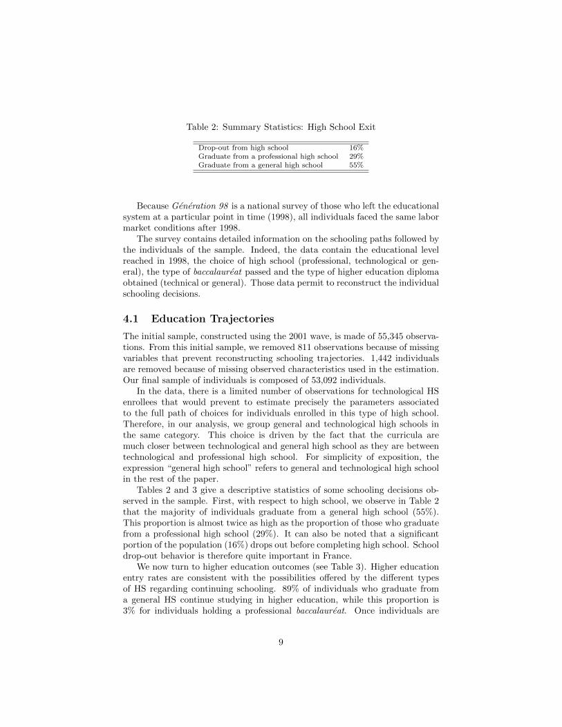
Table 2: Summary Statistics: High School Exit

Drop-out from high school 16%Graduate from a professional high school 29%Graduate from a general high school 55%

Because Generation 98 is a national survey of those who left the educationalsystem at a particular point in time (1998), all individuals faced the same labormarket conditions after 1998.

The survey contains detailed information on the schooling paths followed bythe individuals of the sample. Indeed, the data contain the educational levelreached in 1998, the choice of high school (professional, technological or gen-eral), the type of baccalaureat passed and the type of higher education diplomaobtained (technical or general). Those data permit to reconstruct the individualschooling decisions.

4.1 Education Trajectories

The initial sample, constructed using the 2001 wave, is made of 55,345 observa-tions. From this initial sample, we removed 811 observations because of missingvariables that prevent reconstructing schooling trajectories. 1,442 individualsare removed because of missing observed characteristics used in the estimation.Our final sample of individuals is composed of 53,092 individuals.

In the data, there is a limited number of observations for technological HSenrollees that would prevent to estimate precisely the parameters associatedto the full path of choices for individuals enrolled in this type of high school.Therefore, in our analysis, we group general and technological high schools inthe same category. This choice is driven by the fact that the curricula aremuch closer between technological and general high school as they are betweentechnological and professional high school. For simplicity of exposition, theexpression “general high school” refers to general and technological high schoolin the rest of the paper.

Tables 2 and 3 give a descriptive statistics of some schooling decisions ob-served in the sample. First, with respect to high school, we observe in Table 2that the majority of individuals graduate from a general high school (55%).This proportion is almost twice as high as the proportion of those who graduatefrom a professional high school (29%). It can also be noted that a significantportion of the population (16%) drops out before completing high school. Schooldrop-out behavior is therefore quite important in France.

We now turn to higher education outcomes (see Table 3). Higher educationentry rates are consistent with the possibilities offered by the different typesof HS regarding continuing schooling. 89% of individuals who graduate froma general HS continue studying in higher education, while this proportion is3% for individuals holding a professional baccalaureat. Once individuals are

9

Table 3: Summary Statistics: Higher Education Outcomes

After Aftergeneral professional

high school high schoolHigher education entry rate

Graduate from higher education 89% 3%Stop schooling after high school 21% 97%

Higher education exit level (conditional on higher education entry)General early higher education graduate (baccalaureat and 2 years) 6% 7%Technical early higher education graduate (baccalaureat and 2 years) 38% 81%Intermediate higher education graduate (baccalaureat and 3 or 4 years) 29% 10%Advanced higher education graduate (baccalaureat and 5 years or more) 27% 2%

enrolled in higher education, the vast majority of the ones who graduate froma professional high school get mainly an undergraduate technical degree (81%).Among the individuals who graduate from a general HS, 56% get an intermediateor advanced degree.

4.2 Wage Data

We use wages reported in the first two interview waves (2001 and 2003). Asa consequence, we have access to panel data that cover the first five years ofindividuals working life (from 1998 to 2003). We construct our panel by keepingone monthly wage observation for each year from 1998 to 2003 for full timeemployed individuals. Wages are expressed in 2001 euros. Observations withextreme values of wages have been removed from the sample. Wage descriptivestatistics as well as the number of observations for each year are reported inTable 18 in Appendix A.

5 Structural Model

5.1 Structure of the Educational System

We characterize the education system using three dimensions. One dimensionis purely qualitative and designates the education track (General, Professionalor Technical). The second dimension refers to the level of education (seniorhigh school level or higher education). Finally, the third dimension is the gradelevel and refers to the number of years characterizing any track-level specificcombination. The notation is defined as follows.

• The tracks are: General (G), Professional (P ), Technical (T ). We treatdrop-outs (those who do not attend senior high school) as the outsideoption.

10

• The two levels are denoted as follows: Low (L) which corresponds to lycee(senior high school) and High (H) corresponding to university (highereducation).

• The different grade levels are noted using numbers (1, 2, 3).15

It should be noted that Technical education (corresponding to BTS andDUT ) is only available at higher level (first two years in higher education).So, this means that there is no technical option at the low level. Similarly,the professional track exists only at the lower level. So, to some extent, thetechnical track plays a role similar to the professional track, but only at thehigher education level. General higher education incorporates different gradelevels (1 to 3). Those grades correspond to early higher education graduate(DEUG), intermediate higher education (licence, maitrise) and advanced highereducation (master, doctorat).

5.2 Preferences

The per-period utility functions are meant to capture the consumption values,net of direct costs, associated to each combination of track-level-grade. Onekey contribution of our analysis is the incorporation of switching costs betweentracks. In order to capture the psychic costs (disutility) of switching educationaltracks, we let the utilities of early higher education in the general and technicalsystems to depend on the track attended at the lower educational level (highschool level). Similarly, the utilities of intermediate or advanced higher educa-tion in the general system also depend on the track attended at the early highereducation level.

As a general rule, we use a superscript s to distinguish per-period utilities ofschool from employment and the remaining superscripts to index the tracks, thelevels and the grades. Each per-period utilities depend on observed heterogene-ity, measured by a vector of characteristics Xi, and on an unobserved specifictaste for each specific educational sector {θGi , θPi , θTi }.

The list of observed covariates is composed by parents occupation, parentscountry of origin, a dummy for living in an urban area, a dummy indicating ifthe individual has been delayed at school before grade 6 and a gender dummy.Summary statistics can be found in Table 18 in Appendix A.

We first document the notation for the utilities of attending senior-highschool (the low level). For those utilities, there is no grade dimension.16

15The level dimension is specific to higher education. No grade dimension is considered atthe high school level (see below).

16The outside option category (drop-out from high school) corresponds to decisions of stop-ping education before completing senior high-school, whatever the number of years of educa-tion completed.

11

High school (Low level, L)

The utility of general education at high school (low) level is denoted

Us,GLit = Xiβ

GL + θGi + εs,GLit .

The utility of professional education at high school level is denoted

Us,PLit = Xiβ

PL + θPi + εs,PLit ,

where εs,GLit and εs,PL

it are stochastic utility shocks. Their distribution is docu-mented below.

Finally, the utility of the drop-out (outside) option is set to 0.

Higher Education (High level, H)

The utility of attending general higher education (at grade 1) is denoted

Us,GH1it = Xiβ

GH + θGi + δGP · 1(prof. high school) + δG1 + εs,GH1it ,

where 1(prof. high school) is an indicator equal to 1 when one has attendedprofessional high school. The parameter δGP is a utility shifter that measuresthe disutility switching cost for those who started in the professional track andswitched to a general program. δG1 is an intercept specific to grade 1 in generalhigher education.

The utility of attending technical higher education (at grade 1) is denoted

Us,TH1it = Xiβ

TH + θTi + δTP · 1(prof. high school) + εs,THit ,

where δTp measures the cost of switching from professional to technical.The utility of attending general higher education (at grade 2) is denoted

Us,GH2it = Xiβ

GH + θGi + δGT · 1(tech. early HE) + δG2 + εs,GH2it ,

where 1(tech. early HE) is an indicator equal to 1 when one has attended tech-nical education in grade 1 and δGT measures the cost of switching from technicalto general. Finally, δG2 measures the change in utility of attending a highergrade level.

The utility of attending general higher education (at grade 3) is denoted

Us,GH3it = Xiβ

GH + θGi + δGT · 1(tech. early HE) + δG3 + εs,GH3it ,

where δG3 (like δG2 ) measures changes in utility when progressing to a highergrade level.

εs,GH1it , εs,TH

it , εs,GH2it and εs,GH3

it are stochastic utility shocks.Finally, we assume that all the utility shocks are i.i.d. and follow a type 1

extreme value distribution (Rust, 1987).

12

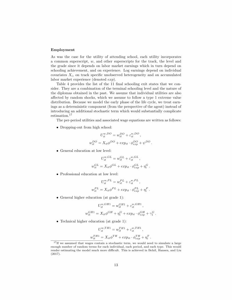
Employment

As was the case for the utility of attending school, each utility incorporatesa common superscript, w, and other superscripts for the track, the level andthe grade since it depends on labor market earnings which in turn depend onschooling achievement, and on experience. Log earnings depend on individualcovariates Xi, on track specific unobserved heterogeneity and on accumulatedlabor market experience (denoted exp).

Table 4 provides the list of the 11 final schooling exit states that we con-sider. They are a combination of the terminal schooling level and the nature ofthe diplomas obtained in the past. We assume that individual utilities are alsoaffected by random shocks, which we assume to follow a type 1 extreme valuedistribution. Because we model the early phase of the life cycle, we treat earn-ings as a deterministic component (from the perspective of the agent) instead ofintroducing an additional stochastic term which would substantially complicateestimation.17

The per-period utilities and associated wage equations are written as follows:

• Dropping-out from high school:

Uw,DOit = wDO

it + εw,DOit ,

wDOit = Xitφ

DO + expit · φDOexp + ψDO .

• General education at low level:

Uw,GLit = wGL

it + εw,GLit ,

wGLit = Xitφ

GL + expit · φGLexp + ηGi .

• Professional education at low level:

Uw,PLit = wPL

it + εw,PLit ,

wPLit = Xitφ

PL + expit · φPLexp + ηPi .

• General higher education (at grade 1):

Uw,GH1it = wGH1

it + εw,GH1it ,

wGH1it = Xitφ

GH + ηGi + expit · φGHexp + γG1 .

• Technical higher education (at grade 1):

Uw,TH1it = wTH1

it + εw,TH1it ,

wTH1it = Xitφ

TH + expit · φTHexp + ηTi .

17If we assumed that wages contain a stochastic term, we would need to simulate a largeenough number of random terms for each individual, each period, and each type. This wouldrender estimating the model much more difficult. This is achieved in Belzil, Hansen, and Liu(2017).

13

Tab

le4:

Fin

al

Sch

ool

Exit

Lev

els

Nam

eof

level

Yea

rsof

Mod

eln

ota

tion

sed

uca

tion

Tra

ckL

evel

Gra

de

Refe

ren

ce

cate

gory

fin

al

level

HS

dro

p-o

ut

0D

O-

-F

inal

levels

aft

er

profe

ssio

nal

secon

dary

ed

ucati

on

Pro

fess

ion

al

HS

gra

du

ate

2P

L-

Tec

hn

ical

earl

yH

Egra

du

ate

aft

erp

rofe

ssio

nal

HS

4T

H1

Gen

eral

earl

yH

Egra

du

ate

aft

erp

rofe

ssio

nal

HS

4G

H1

Fin

al

levels

aft

er

gen

eral

secon

dary

ed

ucati

on

Gen

eral

HS

gra

du

ate

2G

L-

Tec

hn

ical

earl

yH

Egra

du

ate

aft

ergen

eral

HS

4T

H1

Gen

eral

earl

yH

Egra

du

ate

aft

ergen

eral

HS

4G

H1

Inte

rmed

iate

HE

gra

du

ate

aft

ergen

eral

HS

an

dte

chn

ical

earl

yH

E5

GH

2In

term

edia

teH

Egra

du

ate

aft

ergen

eral

HS

an

dgen

eral

earl

yH

E5

GH

2A

dvan

ced

HE

gra

du

ate

aft

ergen

eral

HS

an

dte

chn

ical

earl

yH

E7

GH

3A

dvan

ced

HE

gra

du

ate

aft

ergen

eral

HS

an

dgen

eral

earl

yH

E7

GH

3

Note

:H

Sst

an

ds

for

“H

igh

Sch

ool”

,H

Est

an

ds

for

“H

igh

erE

du

cati

on

”.

14

• General higher education (at grade 2):

Uw,GH2it = wGH2

it + εw,GH2it ,

wGH2it = Xitφ

GH + expit · φGHexp + ηGi + γG2 .

• General higher education (at grade 3):

Uw,GH3it = wGH3

it + εw,GH3it ,

wGH3it = Xitφ

GH + expit · φGHexp + ηGi + γG3 .

The unobserved heterogeneity terms ηGi , ηPi and ηTi represent unobserved

market abilities in track-specific jobs and are the market pendants of the vectorof unobserved taste for each specific track {θGi , θPi , θTi }. The parameters tobe estimated may be grouped as follows: φDO, φGL, φPL, φGH , φTH measurethe impact of observed heterogeneity on earnings for each education class andψDO is the intercept term of the drop-out wage equation. Finally, γG1 , γG2 , γG3are parameters measuring the effect of grade level (within the higher educationgeneral system) on earnings.

5.3 Observed Wages

To close the model, we assume that observed wages, wit, are measured witherror. They are the sum of a deterministic part, denoted wit, and which isused by the agent to take decisions, and a measurement error term, denoted εit.Formally, we have that

wfit = wf

it + εfit for f = DO,GL, ...GH2, GH3 ,

where we assume that εfit ∼ N (0, σf ) and are independent across i, t and f .

5.4 Value Functions

Because the data do not allow us to observe discontinuous schooling-employmentpatterns, we must assume that employment is a terminal state. The valuefunctions of the work options are composed of the sum of discounted expectedutilities of working assuming a constant earnings growth rate which depends oneducational outcome.

In order to characterize the value functions of leaving the educational systemfor employment, we first set a terminal date, denoted T , corresponding to 30years of age. As an example, this means a total time horizon of 14 years in totalfor someone dropping-out from high school. To set the value functions, we usethe standard number of years of education to attain each education level (yearsof education are shown in Table 4).

15

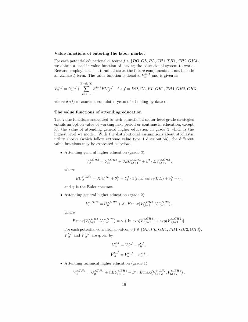
Value functions of entering the labor market

For each potential educational outcome f ∈ {DO,GL,PL,GH1, TH1, GH2, GH3},we obtain a specific value function of leaving the educational system to work.Because employment is a terminal state, the future components do not includean Emax(.) term. The value function is denoted V w,f

it and is given as

V w,fit = Uw,f

it +

T−df (t)∑j=t+1

βj−1EUw,fij for f = DO,GL,PL,GH1, TH1, GH2, GH3 ,

where df (t) measures accumulated years of schooling by date t.

The value functions of attending education

The value functions associated to each educational sector-level-grade strategiesentails an option value of working next period or continue in education, exceptfor the value of attending general higher education in grade 3 which is thehighest level we model. With the distributional assumptions about stochasticutility shocks (which follow extreme value type 1 distribution), the differentvalue functions may be expressed as below.

• Attending general higher education (grade 3):

V s,GH3it = Us,GH3

it + βEUs,GH3i,t+1 + β2 · EV w,GH3

i,t+2 ,

where

EUs,GH3it = Xiβ

GH + θGi + δGT · 1(tech. early HE) + δG3 + γ ,

and γ is the Euler constant.

• Attending general higher education (grade 2):

V s,GH2it = Us,GH2

it + β · Emax(V s,GH3i,t+1 , V w,GH2

i,t+1 ) ,

where

Emax(V s,GH3i,t+1 , V w,GH2

i,t+1 ) = γ + ln[exp(Vs,GH3

i,t+1 ) + exp(Vw,GH2

i,t+1 )] .

For each potential educational outcome f ∈ {GL,PL,GH1, TH1, GH2, GH3},V

s,f

it and Vw,f

it are given by

Vs,f

it = V s,fit − ε

s,fit ,

Vw,f

it = V w,fit − εw,f

it .

• Attending technical higher education (grade 1):

V s,TH1it = Us,TH1

it + βEUs,TH1i,t+1 + β2 · Emax{V s,GH2

i,t+2 , V w,TH1i,t+2 } .

16

• Attending general higher education (grade 1):

V s,GH1it = Us,GH1

it + βEUs,GH1i,t+1 + β2 · Emax{V s,GH2

i,t+2 , V w,GH1i,t+2 } .

• Professional education at low level:

V s,PLit = Us,PL

it + βEUs,PLi,t+1 + β2 · Emax{V s,GH1

i,t+2 , V s,TH1i,t+2 , V w,PL

i,t+2 } .

• General education at low level:

V s,GLit = Us,GL

it + βEUs,GLi,t+1 + β2 · Emax{V s,GH1

i,t+2 , V s,TH1i,t+2 , V w,GL

i,t+2 } .

As in Rust (1987), choice probabilities at each decision node obey the logisticform. In order to build the likelihood function of observed education outcomesand trajectories, we write down the probabilities of each schooling path chosen.This set of probabilities defines all possible educational trajectories that thedata allow us to identify. To build the likelihood, we define a vector Hi thatrecords the highest grade attainment as well as all relevant information relevantto individual trajectories. In Appendix B, we reproduce all choice probabilitiesthat are used in to obtain individual contributions to the likelihood and whichexhaust all possible outcomes for Hi.

5.5 The Likelihood

The contribution to the likelihood for an individual has two components: thefirst component corresponds to the schooling decisions and the second partcorresponds to the wages.

For schooling decisions, the individual contribution to the likelihood is theprobability associated to the observed schooling path. This contribution, de-noted Pr(Hi = hi), is built from the relevant transition probabilities and de-pends onXi as well as on the vector of unobserved heterogeneity (θGi , θ

Pi , θ

Ti , η

Gi , η

Pi , η

Ti ).

For observed wages, the contribution to the likelihood for individual i, con-ditional on history hi, is given by

LW (wit | Hi, Xi, ηGi , η

Pi , η

Ti ) =

T∏t=1

Pr(wit|Hi, Xi,, ηGi , η

Pi , η

Ti )1(eit=1) ,

where Pr(wit|Hi, Xi,, ηGi , η

Pi , η

Ti ) is the wage density at period t and eit is an

indicator equal to 1 if individual i is full-time employed at period t.The total individual likelihood, conditional on unobserved type, is:

Li(Hi, wit;Xi, θGi , θ

Pi , θ

Ti , η

Gi , η

Pi , η

Ti ) = Pr(Hi = hi|Xi, θ

Gi , θ

Pi , θ

Ti , η

Gi , η

Pi , η

Ti ) ·

T∏t=1

Pr(wi,t,|Hi, Xi,, ηGi , η

Pi , η

Ti )1(ei,t=1) .

17

The distribution for the individual specific unobserved heterogeneity is ap-proximated with a discrete distribution. Therefore, assuming that there are Mtypes of individuals, each type m is endowed with the following set:

(θGm, θPm, θ

Tm, η

Gm, η

Pm, η

Tm) for m = 1, . . . ,M ,

where the type probabilities are specified as logistic transforms:

pm =exp(qm)∑M

m=1 exp(qm)m = 1, . . . ,M ,

where qm’s are parameters to be estimated, with the restriction that qM = 0.The mixed likelihood for an individual i is given by

Li(·) =

M∑m=1

pm · Lim ,

where Lim is the likelihood conditional on type m.The model is estimated by maximization of the sum of all individual log

likelihoods.

6 Empirical Results

As a first step, we estimated the model with 4 types (a relatively standardnumber in the structural literature) and also considered larger numbers. Wefound that the improvements in model fit beyond 5 types were marginal. Forthis reason, we base our presentation of the results on the specification with 5types. The discount factor β is fixed to 0.95.

The list of observed covariates, represented by the vector X in the model, iscomposed by parents occupation, parents country of origin, a dummy for livingin an urban area, a dummy indicating if the individual has been delayed atschool before grade 6 and a gender dummy. Summary statistics can be foundin Table 18 in Appendix A.

The model with 5 types contains 191 parameters. However, and as is oftenthe case in complicated non-linear models, many parameters do not raise specificinterest. For this reason, we base our presentation mostly on simulations of alarge number of individual trajectories reflecting the distribution of types andstochastic shocks and use simulated data to analyze the main properties of themodel. This sample constitutes our control group which will be used later toevaluate the cost of raising professional high school attendance. All structuralparameter estimates can be found in Appendix C, Tables 20 to 25.

6.1 Model fit

In a first set of tables (Tables 5, 6 and 7), we compare predicted outcomes withfrequencies observed in the data. We investigate the capacity of our model to

18

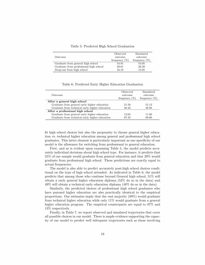
Table 5: Predicted High School Graduation

Observed SimulatedOutcome outcome outcome

frequency (%) frequency (%)Graduate from general high school 54.81 55.05Graduate from professional high school 29.01 29.29Drop-out from high school 16.18 15.65

Table 6: Predicted Early Higher Education Graduation

Observed SimulatedOutcome outcome outcome

frequency (%) frequency (%)After a general high school

Graduate from general early higher education 51.58 51.12Graduate from technical early higher education 48.42 48.88

After a professional high schoolGraduate from general early higher education 12.65 11.00Graduate from technical early higher education 87.35 89.00

fit high school choices but also the propensity to choose general higher educa-tion vs. technical higher education among general and professional high schoolgraduates. This latter element is particularly important as one specificity of ourmodel is the allowance for switching from professional to general education.

First, and as is evident upon examining Table 5, the model predicts accu-rately individual decisions about high school type. For instance, it predicts that55% of our sample would graduate from general education and that 29% wouldgraduate from professional high school. These predictions are exactly equal toactual frequencies.

The model is also able to predict accurately post-high school choices condi-tional on the type of high school attended. As indicated in Table 6, the modelpredicts that among those who continue beyond General high school, 51% willobtain a early general higher education diploma (52% do so in the data) and49% will obtain a technical early education diploma (48% do so in the data).

Similarly, the predicted choices of professional high school graduates whohave pursued higher education are also practically identical to the empiricalproportions. Our estimates imply that the vast majority (89%) would graduatefrom technical higher education while only 11% would graduate from a generalhigher education program. The empirical counterparts are equal to 87% and13% respectively.

Finally, in Table 7, we report observed and simulated trajectories that coverall possible choices in our model. There is ample evidence supporting the capac-ity of our model to predict well infrequent trajectories such as those involving

19

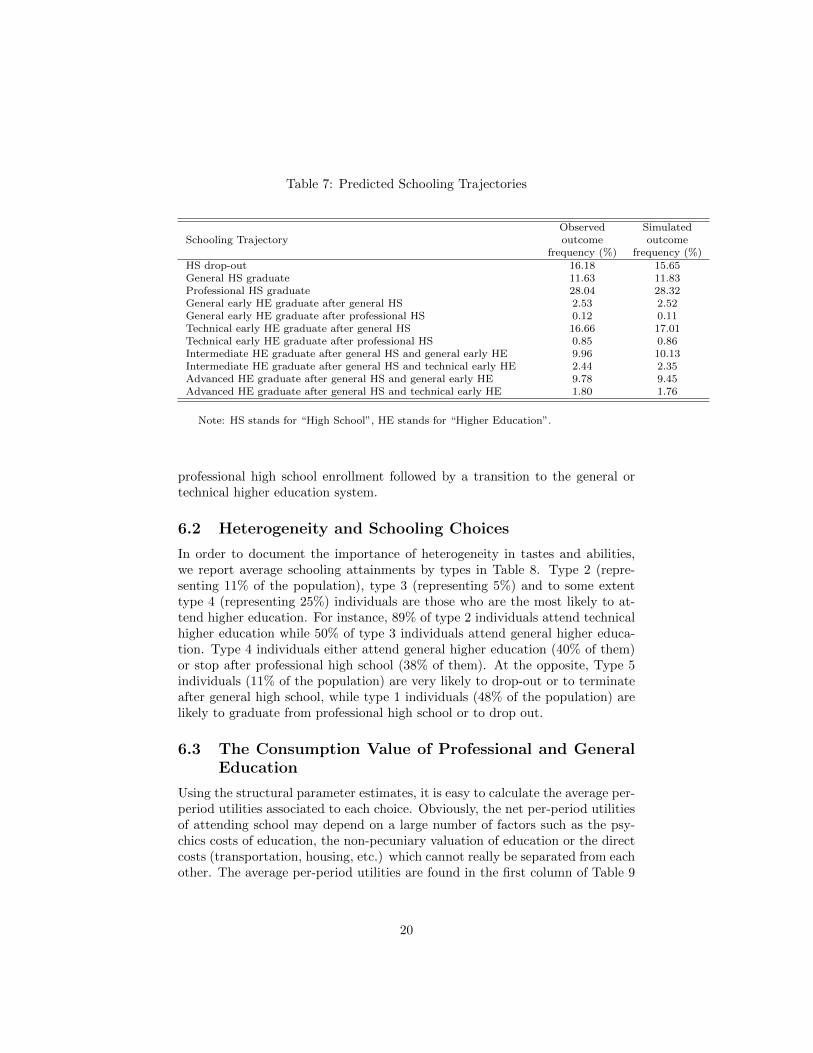
Table 7: Predicted Schooling Trajectories

Observed SimulatedSchooling Trajectory outcome outcome

frequency (%) frequency (%)HS drop-out 16.18 15.65General HS graduate 11.63 11.83Professional HS graduate 28.04 28.32General early HE graduate after general HS 2.53 2.52General early HE graduate after professional HS 0.12 0.11Technical early HE graduate after general HS 16.66 17.01Technical early HE graduate after professional HS 0.85 0.86Intermediate HE graduate after general HS and general early HE 9.96 10.13Intermediate HE graduate after general HS and technical early HE 2.44 2.35Advanced HE graduate after general HS and general early HE 9.78 9.45Advanced HE graduate after general HS and technical early HE 1.80 1.76

Note: HS stands for “High School”, HE stands for “Higher Education”.

professional high school enrollment followed by a transition to the general ortechnical higher education system.

6.2 Heterogeneity and Schooling Choices

In order to document the importance of heterogeneity in tastes and abilities,we report average schooling attainments by types in Table 8. Type 2 (repre-senting 11% of the population), type 3 (representing 5%) and to some extenttype 4 (representing 25%) individuals are those who are the most likely to at-tend higher education. For instance, 89% of type 2 individuals attend technicalhigher education while 50% of type 3 individuals attend general higher educa-tion. Type 4 individuals either attend general higher education (40% of them)or stop after professional high school (38% of them). At the opposite, Type 5individuals (11% of the population) are very likely to drop-out or to terminateafter general high school, while type 1 individuals (48% of the population) arelikely to graduate from professional high school or to drop out.

6.3 The Consumption Value of Professional and GeneralEducation

Using the structural parameter estimates, it is easy to calculate the average per-period utilities associated to each choice. Obviously, the net per-period utilitiesof attending school may depend on a large number of factors such as the psy-chics costs of education, the non-pecuniary valuation of education or the directcosts (transportation, housing, etc.) which cannot really be separated from eachother. The average per-period utilities are found in the first column of Table 9

20

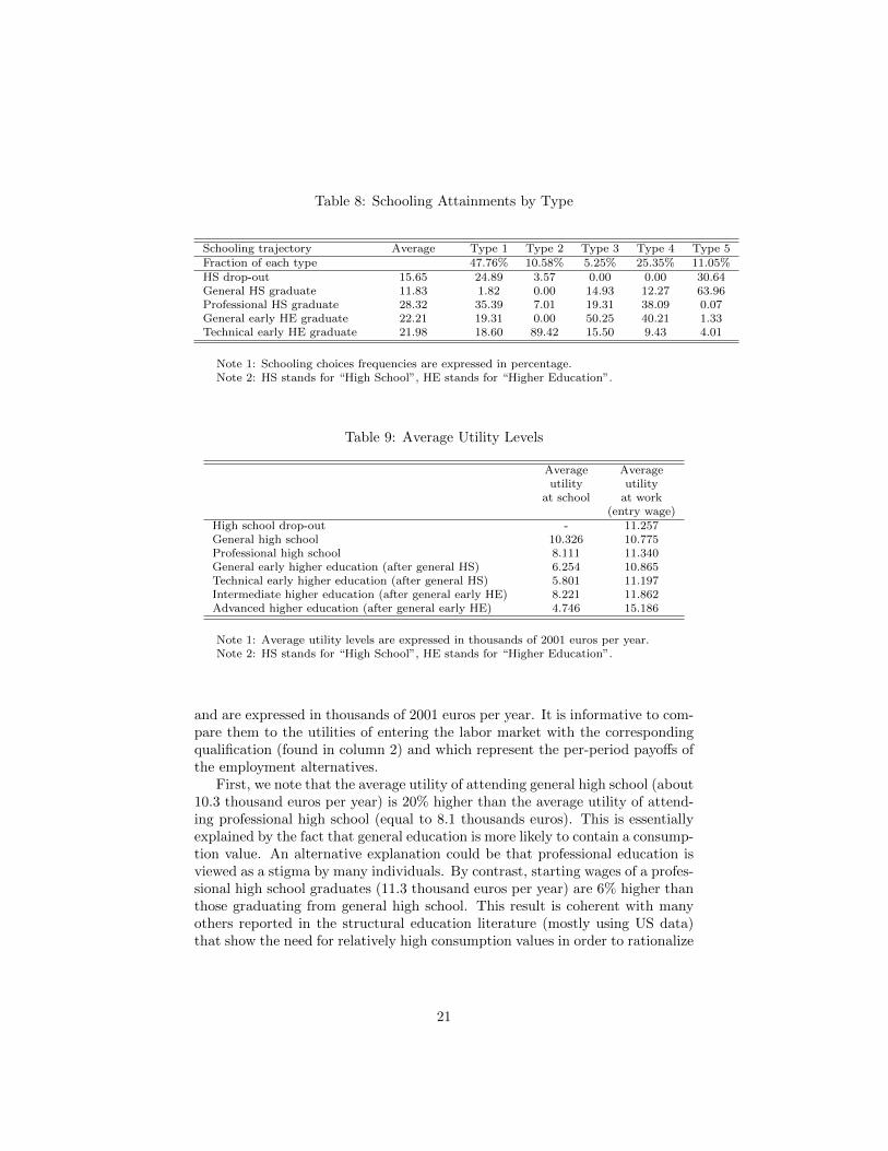
Table 8: Schooling Attainments by Type

Schooling trajectory Average Type 1 Type 2 Type 3 Type 4 Type 5Fraction of each type 47.76% 10.58% 5.25% 25.35% 11.05%HS drop-out 15.65 24.89 3.57 0.00 0.00 30.64General HS graduate 11.83 1.82 0.00 14.93 12.27 63.96Professional HS graduate 28.32 35.39 7.01 19.31 38.09 0.07General early HE graduate 22.21 19.31 0.00 50.25 40.21 1.33Technical early HE graduate 21.98 18.60 89.42 15.50 9.43 4.01

Note 1: Schooling choices frequencies are expressed in percentage.Note 2: HS stands for “High School”, HE stands for “Higher Education”.

Table 9: Average Utility Levels

Average Averageutility utility

at school at work(entry wage)

High school drop-out - 11.257General high school 10.326 10.775Professional high school 8.111 11.340General early higher education (after general HS) 6.254 10.865Technical early higher education (after general HS) 5.801 11.197Intermediate higher education (after general early HE) 8.221 11.862Advanced higher education (after general early HE) 4.746 15.186

Note 1: Average utility levels are expressed in thousands of 2001 euros per year.Note 2: HS stands for “High School”, HE stands for “Higher Education”.

and are expressed in thousands of 2001 euros per year. It is informative to com-pare them to the utilities of entering the labor market with the correspondingqualification (found in column 2) and which represent the per-period payoffs ofthe employment alternatives.

First, we note that the average utility of attending general high school (about10.3 thousand euros per year) is 20% higher than the average utility of attend-ing professional high school (equal to 8.1 thousands euros). This is essentiallyexplained by the fact that general education is more likely to contain a consump-tion value. An alternative explanation could be that professional education isviewed as a stigma by many individuals. By contrast, starting wages of a profes-sional high school graduates (11.3 thousand euros per year) are 6% higher thanthose graduating from general high school. This result is coherent with manyothers reported in the structural education literature (mostly using US data)that show the need for relatively high consumption values in order to rationalize

21

education choices.18

The per-period utility differential between general and professional atten-dance may be particularly interesting in light of the debate regarding the im-portance of the consumption value. In the structural literature, it is difficult toseparate from other elements affecting the per-period utility. However, in thepresence of two parallel systems which are both free of tuition (French lyceesdo not charge any tuition), the utility differential may help identify the non-pecuniary elements if one is willing to assume that other elements such as goodsand services consumption while in school and direct costs (such as transporta-tion) are invariant to the type of high school attended. If one assumes furtherthat the consumption value is only present for general education, then one couldinterpret the 20% differential as the share of the total per-period utility of at-tending general high school explained by non-pecuniary elements.

Similarly, the per-period utility differential between general early higher edu-cation and technical higher education, which is equal to 8% ((6,254-5,801)/5,801),may also be explained by a higher consumption value for general higher educa-tion at the upper level.

However, when compared to high school, the utilities of attending the earlyphase of general and technical higher education are somewhat lower (6.3 thou-sand euros and 5.8 thousand euros respectively). Because higher education isalso free in France, this reduction is most likely explained by a certain level ofdisutility setting in when moving toward upper education levels. It is interest-ing to note that entry wages representing the payoffs of the alternative option(to work instead of attending higher education), and which are equal to 10.9thousand euros and 11.2 thousand euros, are much higher than the per-periodutilities of attending education.

While the utility of attending the intermediate level is comparable to theutility of attending general high school (8.2 thousand euros), the utility of ad-vanced higher education is found to be very low (about 4.7 thousand euros peryear), especially when compared to its entry wage pendant equal to 15.2 thou-sand euros. This is most likely explained by an increasing level of disutilityfor higher education as one progresses from intermediate to advanced levels. Inturn, this disutility could reflect pure aging effects or heavier psychic costs ofeducational investments when reaching advanced levels.

In Table 10, we report the average utilities of attending education for eachtype.

The utilities are particularly dispersed at higher education attendance level.First, the utilities of attending general high school range from 6059 euros for type2 to 15,000 euros for type 3, while for professional high school, the range is from4274 euros (type 2) to 11220 euros (for type 4). However, for general early highereducation, the lowest utility is 1980 euros (type 2) while the highest one is 10,934euros (for type 3). It is interesting to note that type 1 individuals who representalmost half of the population are endowed with an average utility almost equal to

18See Keane and Wolpin (1997) for a seminal piece. The structural literature is surveyed inBelzil (2007).

22

Table 10: Average Schooling Utility Levels by Type

Type 1 Type 2 Type 3 Type 4 Type 5Fraction of each type 47.76% 10.58% 5.25% 25.35% 11.05%General high school 10.282 6.059 14.999 12.078 8.357Professional high school 7.134 4.274 10.148 11.220 7.905General early higher education (after general HS) 6.212 1.980 10.934 8.007 4.285Technical early higher education (after general HS) 5.404 1.927 10.528 7.402 5.309

Note 1: Average utility levels are expressed in thousands of 2001 euros per year.Note 2: HS stands for “High School”.

the population average (6,212 euros) and also that none of the types is endowedwith a per-period utility of education that is at least as large at the average entrywage of high school graduates (about 11,000 euros). It is helpful to compare ourestimates to the distribution of the period utility of attending college reportedin Keane and Wolpin (1997). These authors essentially report that the felicityof attending college is well above the average earnings of young American malesaged 18 for a significant portion of the population and also much below foranother significant share. This therefore suggests that the consumption valueof higher education is less dispersed in France than in the US.19

6.4 The Costs of Switching Tracks

One specificity of the French education system is that it is meant to facilitate (orat least render possible) movements from one track to another. However, suchmovements are relatively uncommon. For instance, and among professional HighSchool graduates, only 3% will eventually graduate from early higher education,and they do so almost exclusively in a technical program. Movements acrosstracks are substantially more frequent in higher education. Among individualswho graduate from technical early higher education, 20% switch to generalintermediate higher education while 80% decide to enter the labor market.

Our model explains the relatively scarce movements from professional highschool to general higher education as we allow for an extra-disutility term affect-ing the utility of attending higher education when coming from the professionalsystem. In total, there are 3 instances where switching costs may be acting.The results, found in Table 11 indicate clearly the movement from a profes-sional high school to general early higher education is by far the most costly interms of per-period utilities. Our estimate, equal to -1.34 thousand euros peryear, implies a 21.5% reduction in the utility of attending general higher edu-cation for a randomly chosen individual who would have attended professional

19As an illustration, Keane and Wolpin (1997) report that the utility of attending schoolmay be as high as $15,000 for the high schooling types whereas the average yearly wage atcomparable age may be between $10,000 and $11,000.

23

Table 11: Utility Shifts Induced by Track Switching

Parameter PercentageType of track switching estimate of utility

shiftSwitching from professional secondary education -1.343 -21.48%to general early higher education

Switching from professional secondary education 0.099 1.71%to technical early higher education

Switching from technical early higher education -0.092 -1.11%to general intermediate higher education

education. This essentially means that switching to a general track removes asubstantial fraction of the consumption value of general education.

Switching from technical early education to the general track (at the inter-mediate level) appears to be costly as well, but much less than moving from aprofessional high school. Its cost, which is about 90 euros per year, representsonly a 1.1% drop in the per-period utility of attending.

It is however interesting to note that moving from the professional trackto the technical early higher education track provides a positive shift of 100euros per year and corresponds to a 1.71% increase in utility. This most likelyindicates that the professional high school academic curriculum is adequate topermit the average student in the population to enter technical education.

6.5 Sources of Selectivity

One interesting question is to what extent individual heterogeneity is explainedby observed family background characteristics as opposed to unobserved het-erogeneity. We first decompose the relative contributions of observed and unob-served heterogeneity to the initial track decision. The results, shown in Table 12,indicate that observed and unobserved heterogeneity are close to play an equallybalanced role as observed characteristics account for 52% of total heterogeneityand unobserved heterogeneity accounts for 48%. However, it is equally inter-esting to note that after conditioning on the initial track, the importance ofobserved family characteristics practically vanishes as unobserved heterogeneityabsorbs more than 95% of the explained variations in education decision.

7 Measuring the Option Values of Professionaland General Education

The structure of our model allows us to measure two different components ofthe returns to schooling. One component is qualitative since it attempts tomeasure differences in wages explained by different tracks given the same length

24

Table 12: Variance Decomposition of Track Choices

Track choice Track choicein secondary in early higher

education educationObserved heterogeneity 52% 4%Unobserved heterogeneity 48% 96%

Table 13: Qualitative Returns to the Type of Secondary Education

Entry wages Wages 5 years afterlabor market entry

ATE ATT ATE ATTGeneral high school graduate ref. ref. ref. ref.

Professional high school graduate 0.054∗∗∗ 0.062∗∗∗ 0.062∗∗∗ 0.070∗∗∗

(0.002) (0.002) (0.002) (0.002)

Note 1: Standard errors under parenthesis. Significance levels: ∗∗∗ 1%; ∗∗ 5%; ∗ 10%.Note 2: The returns are conditional on leaving school after high school graduation.

of education. The second refers to the classical return to an extra year ofeducation (given track) and is particularly relevant for the general track sincethe professional track is short and leads to market entrance in young age. Wenow analyze both.

7.1 Qualitative Returns: The Distinction between Profes-sional and General Education

We define the qualitative component of the returns to schooling as the differencein mean wages between professional and general education graduates who haveinvested the same number of years. To obtain it, we therefore compute expectedwages conditional on stopping after completing the secondary level (around age18) for both options. Differences in mean wages are therefore solely due tothe qualitative nature of the education curriculum. The estimates are foundin Table 13. Because our model allows for a causal effect of education on thepost-schooling growth rate, we present estimates obtained using entry wages aswell as estimates obtained 5 years after labor market entry.

Using simulated outcomes, it is also possible to differentiate between theaverage return in the population (designated as ATE in Table 13) and theaverage return for those having chosen the treatment (designated by ATT inTable 13).

First, the positive estimate for the ATE on entry wages, and equal to 0.054,indicates that conditional on stopping after high school, professional educationgenerates higher wages than general education. This may simply reflect the fact

25

that a general high school education curriculum builds up skills that are mostlyuseful at stimulating subsequent skill accumulation but that are not highlyrewarded in the labor market. Note also that this positive differential is not anartifact driven by selectivity since it is computed over the entire population.

After conditioning on professional education being the optimal choice, thedifference in mean wages of those who actually chose professional education andtheir mean counterfactual wages had they chosen general education (the ATT)is equal 0.062 and is therefore compatible with the existence of comparativeadvantages. This essentially means that those who work after a professional highschool degree are better at performing tasks related to this sort of educationthan the average person in the population.

Finally, it is also important to remark that the positive wage premium infavor of those graduating from professional high school does not vanish oncepost-schooling experience sets in. Both the ATE estimate (0.062) and the ATTestimate (0.070) measuring the wage differential 5 years beyond labor marketentrance remain positive and indicate that professional high school graduatesstill outperform general high school graduates after entering the market.

7.2 Quantitative Returns

Because professional education is terminal for most people who choose it, it ismore logical to measure quantitative returns for the general/technical tracksonly. As our model is meant to capture heterogeneity across high school tracksbut does not introduce additional heterogeneity for higher education, we onlyconsider average quantitative returns in the population and ignore the distinc-tion between average treatment effects and treatment for the treated.

In order to compute those returns, we use general high school graduation as abenchmark and therefore compare expected wages at various levels to expectedwages obtained upon general high school graduation. It is also important toremember that there is a fundamental asymmetry between general and techni-cal education in that technical education is only an option at the initial stageof higher education while general higher education offers three distinct stages(early, intermediate and advanced).

First, the results found in Table 14 indicate clearly that return to early gen-eral higher education when measured at entry in the market (equal to 0.008)is below the return to a technical degree (equal to 0.044) but exceeds it after5 years. That is when incorporating differences in returns to experience be-tween general and technical education, the benefit of a general early educationdegree reaches almost 15% (the estimate is 0.146) while the benefit attached toa technical degree is below 10% (the estimate is 0.093).

As is the case for the US, the returns to general education are highly convex.The financial return to the first two years of general education is practicallyequal to 0 (0.008) but completing a third year (obtaining an intermediate highereducation diploma) raises wages by almost 10% compared to a general highschool graduate (0.096). This implies an average return of 3% per year ofschooling over the first 3 years. However, completing 5 years has a significant

26

Table 14: Quantitative Returns after General Secondary Education

Entry Wages 5 yearsEducational outcome wages after labor

market entryGeneral high school graduate ref. ref.

General early higher education graduate (2 years) 0.008∗∗∗ 0.146∗∗∗

(0.003) (0.003)

Technical early higher education graduate (2 years) 0.044∗∗∗ 0.093∗∗∗

(0.005) (0.005)

Intermediate higher education graduate (3 years) 0.096∗∗∗ 0.233∗∗∗

(0.003) (0.003)

Advanced higher education graduate (5 years) 0.343∗∗∗ 0.480∗∗∗

(0.004) (0.006)

Note 1: Standard errors under parenthesis. Significance levels: ∗∗∗ 1%; ∗∗ 5%; ∗ 10%.Note 2: Years of schooling are indicated in deviation to high school graduation.

impact as the differential with a high school graduate raises to 34% (0.343).Those numbers imply marginal returns of 12% per year of schooling over thelast 2 years. When averaged over 5 years, the return to general education raisesto about 7% per year of schooling and therefore reaches a value comparable tothose reported for the US (Belzil, 2007). However, it is clear that the financialbenefit of general higher education is only reaped at the end of the curriculum.

It is important to note that the returns to technical higher education arereaped earlier than those of general education. The wage differential betweena person completing two years of technical higher education and a general highschool graduate, equal to 4.4%, implies an average return of 2% per year in theearly phase.

Finally, we find that a fair portion of the return to general education isreaped in terms of post-education wage growth. After 5 years of experience,those who have obtained an advanced higher education degree would earn 48%more than general high school graduates. This means that after 5 years oflabor market experience, about 30% of the return to schooling is explained bydifferences in the slope of early career age earnings profiles.

7.3 The Option Value of General and Professional Educa-tion

The convexity of the wage schooling relationship (within the general track),along with the relatively high cost of switching from the professional to thegeneral track, suggest that one major reason for enrolling in general educationin high school is a significant option value. To clarify this point, we measurethe option value associated to each type of school. More precisely, we computethe difference between the lifetime utility gain (until age 30) of completing

27

Table 15: Option Value of the Type of Secondary Education

Option value Option valueof of

general professionalhigh school high school

Total utility gain (consumption value of schooling and wages) 7.715 -1.334Wage gain -15.282 -11.432

Note 1: Utility levels and wages are expressed in thousands of 2001 euros per year.Note 2: The option value is calculated as the average difference in the sum of discounted

lifetime utility flows between individuals who stop schooling at the secondary education leveland individuals who stop schooling at a more advanced level (higher education).

professional education and the lifetime utility gain of entering the labor marketafter professional education. We proceed similarly for general education. Toobtain a feeling of the importance of the consumption value of education, wealso measure option values after removing the schooling utility components.This measure allows us to quantify the relative importance of forgone earningsand especially to what extent individuals involved in higher education maycompensate the earnings penalty of education by subsequent higher earnings.

Not surprisingly, as shown in Table 15, the option value of entering a generalhigh school track is much higher than its professional counterpart. For thegeneral track, the discounted utility gain realized until age 30 is equal to 7,715euros. This gain is however positive mostly because higher education generatesa consumption value. If we removed the utility components (affecting highereducation attendance) and measured the option value only based in realizedearnings until age 30, the option value becomes negative and equal to -15,282euros. This is explained by the fact that by age 30, total lifetime earnings ofthose attending university are still lower than those of high school graduateswho started to work at age 18.

The option value of attending the professional track is small in absoluteterms but actually negative (-1,334). When incorporating only earnings, it iseven more negative as our estimate is equal to -11,432 euros.

A similar computation maybe carried for the early phase of general highereducation and technical higher education as both of these choices offer the pos-sibility to continue and reach higher levels of general or technical education.Results are found in Table 16. As was the case for both general and pro-fessional high school, the option value of entering general early education ispositive when incorporating the consumption value (4,417 euros) but becomesnegative (-17,692) when only wages are taken into account. It is interesting tonote that technical higher education entails the largest option values as the valueobtained from utility gains reaches 13,689 euros while the wage-based measure isstill negative (-8,608 euros) but smaller in absolute terms than those measured

28

Table 16: Option Value of the Type of Early Higher Education

Option value Option valueof general of technical

early higher early highereducation education

Total utility gain (consumption value of schooling and wages) 4.417 13.689Wage gain -17.692 -8.608

Note 1: Utility levels and wages are expressed in thousands of 2001 euros per year.Note 2: The option value is calculated as the average difference in the sum of discounted

lifetime utility flows between individuals who stop schooling at the secondary education leveland individuals who stop schooling at a more advanced level (higher education).

for general high school, professional high school and general higher education.

8 Evaluating the Cost of Raising ProfessionalHigh School Attendance

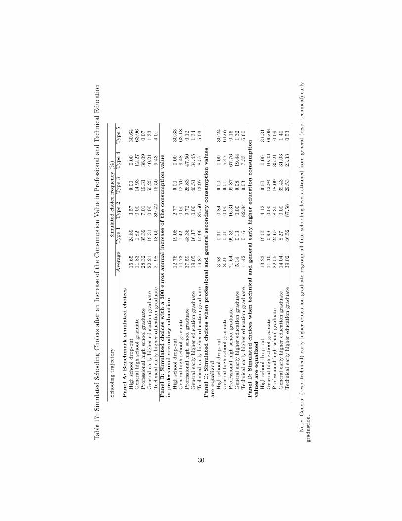
We now turn to the following question: by how much should the per-periodutility of attending professional high school increase if public authorities wishedto raise professional high school enrollments by 10 percentage points? As alreadymentioned, French students tend to favor general education over professionalalternatives. However, many policy analysts claim that professional educationis both under-developed and under-valued in France. There are good reasonsfor that. Public universities tend to be over-crowded and a non-trivial share ofthose entering general higher education drop-out without obtaining any diploma(Gary-Bobo and Trannoy, 2015). As a consequence, tracking those students ill-prepared for general education toward more applied education curricula may bean efficient way to reduce youth-unemployment.

Although the level of the target is intrinsically ad-hoc, we choose a 10 per-centage points increase because it would still leave higher education as the preva-lent option. Such an increase would correspond to a movement from a 28% to38% in professional high school enrollment rates. We are however agnosticabout the method used to achieve this increase. Obviously, an increase in theutility of attending professional high school could be obtained by implementinga subsidy or a cash transfer conditional on enrollment. Other methods, such aspublic information campaigns and the like, could also raise the desirability ofprofessional education by reducing potential stigma attached to it.

To answer this question, we modify the distribution of the per-period util-ities of attending professional high school by calibrating a shift parameter tothe desired enrollment target (38%). Although the utility gap between profes-sional and general high school attendance was found to be as high as 2000 euros

29

Tab

le17

:S

imu

late

dS

chool

ing

Ch

oice

saft

eran

Incr

ease

of

the

Con

sum

pti

on

Valu

ein

Pro

fess

ion

al

an

dT

ech

nic

al

Ed

uca

tion

Sch

oolin

gtr

aje

ctory

Sim

ula

ted

choic

efr

equ

ency

(%)

Aver

age

Typ

e1

Typ

e2

Typ

e3

Typ

e4

Typ

e5

Pan

el

A:

Ben

ch

mark

sim

ula

ted

ch

oic

es

Hig

hsc

hool

dro

p-o

ut

15.6

524.8

93.5

70.0

00.0

030.6

4G

ener

al

hig

hsc

hool

gra

du

ate

11.8

31.8

20.0

014.9

312.2

763.9

6P

rofe

ssio

nal

hig

hsc

hool

gra

du

ate

28.3

235.3

97.0

119.3

138.0

90.0

7G

ener

al

earl

yh

igh

ered

uca

tion

gra

du

ate

22.2

119.3

10.0

050.2

540.2

11.3

3T

ech

nic

al

earl

yh

igh

ered

uca

tion

gra

du

ate

21.9

818.6

089.4

215.5

09.4

34.0

1P

an

el

B:

Sim

ula

ted

ch

oic

es

wit

ha

300

eu

ros

an

nu

al

increase

of

the

con

sum

pti

on

valu

ein

profe

ssio

nal

secon

dary

ed

ucati

on

Hig

hsc

hool

dro

p-o

ut

12.7

619.0

82.7

70.0

00.0

030.3

3G

ener

al

hig

hsc

hool

gra

du

ate

10.7

31.4

20.0

012.7

09.4

863.1

8P

rofe

ssio

nal

hig

hsc

hool

gra

du

ate

37.5

948.3

69.7

226.8

347.5

00.1

2G

ener

al

earl

yh

igh

ered

uca

tion

gra

du

ate

19.0

516.1

70.0

046.5

134.4

51.3

4T

ech

nic

al

earl

yh

igh

ered

uca

tion

gra

du

ate

19.8

714.9

687.5

013.9

78.5

75.0

3P

an

el

C:

Sim

ula

ted

ch

oic

es

wh

en

profe

ssio

nal

an

dgen

eral

secon

dary

con

sum

pti

on

valu

es

are

equ

ali

zed

Hig

hsc

hool

dro

p-o

ut

3.5

80.3

10.8

40.0

00.0

030.2

4G

ener

al

hig

hsc

hool

gra

du

ate

8.2

10.0

10.0

00.0

15.4

761.6

7P

rofe

ssio

nal

hig

hsc

hool

gra

du

ate

71.6

499.3

916.3

199.8

767.7

60.1

6G

ener

al

earl

yh

igh

ered

uca

tion

gra

du

ate

5.1

40.1

30.0

00.0

819.4

41.3

2T

ech

nic

al

earl

yh

igh

ered

uca

tion

gra

du

ate

11.4

20.1

682.8

40.0

37.3

36.6

0P

an

el

D:

Sim

ula

ted

ch

oic

es

wh

en

techn

ical

an

dgen

eral

early

hig

her

ed

ucati

on

con

sum

pti

on

valu

es

are

equ

ali

zed

Hig

hsc

hool

dro

p-o

ut

13.2

319.5

54.1

20.0

00.0

031.3

1G

ener

al

hig

hsc

hool

gra

du

ate

11.1

60.9

80.0

012.9

410.4

366.6

8P

rofe

ssio

nal

hig

hsc

hool

gra

du

ate

22.5

524.6

78.3

018.0

935.2

10.0

9G

ener

al

earl

yh

igh

ered

uca

tion

gra

du

ate

14.0

48.2

70.0

039.4

331.0

31.4

0T

ech

nic

al

earl

yh

igh

ered

uca

tion

gra

du

ate

39.0

246.5

287.5

829.5

323.3

30.5

3

Note

:G

ener

al

(res

p.

tech

nic

al)

earl

yh

igh

ered

uca

tion

gra

du

ate

regro

up

all

fin

al

sch

oolin

gle

vel

satt

ain

edfr

om

gen

eral

(res

p.

tech

nic

al)

earl

ygra

du

ati

on

.

30

(Table 9), reaching a 10 percentage points increase would not require to closethis gap entirely. Simulated schooling choice frequencies, reported in Panel Bof Table 17, indicate that an increase of 300 euros in the utility of attendingprofessional high school would be sufficient to raise enrollments from 28% to38%. They also indicate that an increase of 300 euros would reduce high schooldrop-outs by 3 percentage points (from 16% to 13%). At the same, this realloca-tion in favor of professional high school would be accompanied by a decrease inhigher education enrollments of about 5 percentage points (from 44% to 39%).

To illustrate the importance of the consumption value when choosing anoptimal high school track, we push our analysis further and answer the fol-lowing question: How would schooling decisions change if both utilities wereequalized (while leaving the utilities of general and technical higher educationunchanged)? The resulting frequencies, reported in Panel C of Table 17, il-lustrate the dominant role that per-period utilities play in schooling choices asprofessional enrollments would go from 28% (the benchmark) to 72%. Equal-izing net utilities of attending general and professional high school would alsopractically annihilate the incentive to attend higher education as enrollmentswould fall by 28 percentage points (from 44% to 16%). This may partly be ex-plained by the convexity of the wage-schooling relationship for higher education.Returns to higher education are reaped mostly after attending 5 years of gen-eral higher education while returns to professional high school training exceedthose of general high school for those entering the market at 18. So withouta 20% differential in per-period utilities, about 64% of total higher educationenrollments (28% / 44%) would vanish.

A similar exercise may be performed with early higher education. Recall thatthe average utility of attending general early higher education (6254 euros peryear) is about 8% higher than the average utility of the early phase of generalhigher education (5801 euros per year). As shown in Panel D of Table 17, settingboth utilities equal (while leaving utilities of high school attendance unchanged)would end up doubling technical higher education enrollments (from 22% to39%) and reduce general higher education enrollments by 8 percentage points.As a result, about 75% of all higher education enrollments would be in thetechnical track (39% / 53%).

To summarize, either at the senior high school level or at the higher edu-cation level, the decision to attend general education is largely dominated bynon-pecuniary dimensions. Without it, general education enrollments woulddecrease substantially.

9 Conclusion

We have estimated a structural model of education choices in which individualschoose between a professional and a general track using French panel data. Asis the case for the US, French education choices are also largely driven by non-pecuniary elements and our estimates indicate that this is mostly explained bythe high consumption value of general education. Our findings suggest that pro-

31

fessional education entails higher financial returns for those entering the marketaround age 18, but that investing in general education offers an important op-tion value which can only be reaped after 5 years of higher education. Withouta large positive general-professional utility differential, the incentive to attendgeneral higher education would be dramatically reduced as about 64% of totalhigher education enrollments are explained by the existing general-professionalutility differential. We find that an increase of 300 euros in the net utility ofattending professional high school would be sufficient to increase professionalhigh school enrollments by 10 percentage points.

Our results also suggest avenues for future research. In our model, financialincentives to invest in education are represented by differences in earnings (andearnings growth) across educational outcomes. In actual labor markets, it isconceivable that young individuals also base their decisions on unemploymentoutcome differentials. This suggests that modeling earnings risk through dif-ferential layoff probabilities or unemployment duration may be highly relevant.This is an avenue for future research that we are currently contemplating.

32

References

Adda, J., C. Dustmann, C. Meghir, and J.M. Robin. 2013. “Career Progres-sion, Economic Downturns, and Skills.” Working Paper No. 18832, NationalBureau of Economic Research, February.

Altonji, J.G. 1995. “The Effects of High School Curriculum on Education andLabor Market Outcomes.” The Journal of Human Resources 30:409–438.

Altonji, J.G., P. Arcidiacono, and A. Maurel. 2016. “The Analysis of FieldChoice in College and Graduate School: Determinants and Wage Effects.”Elsevier, vol. 5 of Handbook of the Economics of Education, chap. 7, pp. 305– 396.

Beffy, M., D. Fougere, and A. Maurel. 2012. “Choosing the Field of Studyin Postsecondary Education: Do Expected Earnings Matter?” Review ofEconomics and Statistics 94:334 – 347.

Belzil, C. 2007. “The return to schooling in structural dynamic models: a sur-vey.” European Economic Review 51:1059–1105.

Belzil, C., and J. Hansen. 2002. “Unobserved Ability and the Return to School-ing.” Econometrica 70:2075–2091.

Belzil, C., J. Hansen, and X. Liu. 2017. “Dynamic Skill Accumulation, Educa-tion Policies, and the Return to Schooling.” Quantitative Economics 8:895–927.

Belzil, C., and F. Poinas. 2010. “Education and Early Career Outcomes ofSecond-Generation Immigrants in France.” Labour Economics 17:101–110.

De Groote, O. 2017. “The Effects of High School Curriculum. A Model of Pro-gram and Effort Choice.” Unpublished.

Dustmann, C., P.A. Puhani, and U. Schonberg. 2017. “The Long-term Effectsof Early Track Choice.” The Economic Journal 127:1348–1380.

Eckstein, Z., and K.I. Wolpin. 1999. “Why Youths Drop out of High School: TheImpact of Preferences, Opportunities, and Abilities.” Econometrica 67:1295–1339.

Gary-Bobo, R., and A. Trannoy. 2015. “La Crise du Financement des Univer-sits Franaises: Impot sur le Revenu des Anciens Etudiants ou pret a Rem-boursement Contingent.” In L’universite Desorientee. La Decouverte, no. 16in Regards Croises sur l’Economie.

Gemici, A., and M. Wiswall. 2014. “Evolution of Gender Differences in Post-Secondary Human Capital Investments: College Majors.” International Eco-nomic Review 55:23 – 56.

33

Hanushek, E.A., G. Schwerdt, L. Woessmann, and L. Zhang. 2017. “GeneralEducation, Vocational Education, and Labor-Market Outcomes over the Life-cycle.” Journal of Human Resources 52:48–87.

Heckman, J.J., L. Lochner, and C. Taber. 1998. “Explaining Rising Wage In-equality: Explorations with a Dynamic General Equilibrium Model of LaborEarnings with Heterogeneous Agents.” Review of Economic Dynamics 1:1 –58.

Keane, M.P., and K.I. Wolpin. 1997. “The Career Decisions of Young Men.”The Journal of Political Economy 105:473–522.

—. 2001. “The Effect of Parental Transfers and Borrowing Constraints on Ed-ucational Attainment.” International Economic Review 42:1051 – 1103.

Lee, D., and K.I. Wolpin. 2010. “Accounting for Wage and Employment Changesin the US from 19682000: A Dynamic Model of Labor Market Equilibrium.”Journal of Econometrics 156:68 – 85, Structural Models of Optimization Be-havior in Labor, Aging, and Health.

Meer, J. 2007. “Evidence on the Returns to Secondary Vocational Education.”Economics of Education Review 26:559 – 573.

Rust, J. 1987. “Optimal Replacement of GMC Bus Engines: An EmpiricalModel of Harold Zurcher.” Econometrica 55:999–1033.

34

Appendix

A Descriptive Statistics

Table 18: Summary Statistics: Wage Data

Year Number of Mean Std. dev. Min. Max.observations

1998 25361 1091.39 333.66 646.00 3684.001999 22184 1096.12 318.90 646.77 3792.042000 17346 1105.94 344.81 646.71 3733.492001 39603 1225.03 425.28 646.46 3761.422002 5039 1139.68 351.22 647.66 3665.972003 2076 1113.66 334.64 647.25 3241.79Total/Average 111609 1144.61 373.46 646.00 3792.04

Note: Monthly wages of full-time employed workers, expressed in 2001 euros.

Table 19: Summary Statistics: Observed Characteristics used in the Estimation

Variable MeanFather’s occupation

Tradesman 0.1081Executive 0.1723Technician 0.0841White collar 0.2655Blue collar 0.2752No occupation 0.0947

Mother’s occupationTradesman 0.0414Executive 0.1020Technician 0.0467White collar 0.4818Blue collar 0.1252No occupation 0.2029

Parents’ country of originFrance 0.8016OECD 0.0752Non-OECD 0.1232

Urban location 0.7523Late at school 0.2299Man 0.5131

35

B Choice Probabilities and Educational Trajec-tories

As in Rust (1987), choice probabilities at each decision node obey the logisticform.

At low level, we have the probabilities of choosing

• General low level: P s,GL1,it =

exp(V

s,GL

it

)exp(V

s,GL

it

)+exp

(V

s,PL

it

)+exp

(V

w,DO

it

) ,

• Professional low level: P s,PL1,it =

exp(V

s,PL

it

)exp(V

s,GL

it

)+exp

(V

s,PL

it

)+exp

(V

w,DO

it

) ,

• Drop out (entering the labor market): Pw,DO1,it =

exp(V

w,DO

it

)exp(V

s,GL

it

)+exp

(V

s,PL

it

)+exp

(V

w,DO

it

) .

Conditional on graduating from general high school, we have the probabili-ties of choosing

• General early higher education: P s,GH12,it =

exp(V

s,GH1

it

)exp(V

s,GH1

it

)+exp

(V

s,TH1

it

)+exp

(V

w,GL

it

) ,

• Technical early higher education: P s,TH12,it =

exp(V

s,TH1

it

)exp(V

s,GH1

it

)+exp

(V

s,TH1

it

)+exp

(V

w,GL

it

) ,

• Labor market: Pw,GL2,it =

exp(V

w,GL

it

)exp(V

GH1)+exp

(V

TH1)+exp

(V

w,GL

it

) .

Conditional on graduating from professional high school, we have the prob-ability of choosing

• General early higher education: P s,GH13,it =

exp(V

s,GH1

it

)exp(V

s,GH1

it

)+exp

(V

s,TH1

it

)+exp

(V

w,PL

it

) ,

• Technical early higher education: P s,TH13,it =

exp(V

s,TH1

it

)exp(V

s,GH1

it

)+exp

(V

s,TH1

it

)+exp

(V

w,PL

it

) ,

• Labor market: Pw,PL3,it =

exp(V

w,PL

it

)exp(V

s,GH1

it

)+exp

(V

TH1)+exp

(V

w,PL

it

) .

At the end of general higher education (grade 1), we have the probability ofchoosing

• General higher education (grade 2): P s,GH24,it =

exp(V

s,GH2

it

)exp(V

s,GH2

it

)+exp

(V

w,GH1

it

) ,

• Labor market: Pw,GH14,it =

exp(V

w,GH1

it

)exp(V

s,GH2

it

)+exp

(V

w,GH1

it

) .

36

At the end of technical higher education (grade 1), we have the probabilitiesto choose

• General higher education (grade 2): P s,GH25,it =

exp(V

s,GH2

it

)exp(V

s,GH2

it

)+exp

(V

w,TH1

it

) ,

• Labor market: Pw,TH15,it =

exp(V

w,TH1

it

)exp(V

s,GH2

it

)+exp

(V

w,TH1

it

) .

Finally, at the end of general higher education (grade 2), we have the prob-ability of choosing

• General higher education (grade 3): P s,GH36,it =

exp(V

s,GH3

it

)exp(V

s,GH3

it

)+exp

(V

w,GH2

it

) .

As attending higher education in grade 3 is the highest level in the model,the probability of entering the labor market after completing this grade isequal to the probability of graduating at that level, i.e. Pw,GH3

6 = P s,GH36 .

• Labor market: Pw,GH26,it =

exp(V

w,GH2

it

)exp(V

s,GH3

it

)+exp

(V

w,GH2

it

) .

In order to build the likelihood function of observed education outcomes andtrajectories, we now write down the probabilities of each schooling attainmentand distinguish on the basis of the path chosen. This set of probabilities definesall possible educational trajectories that the data allow us to identify. To buildthe likelihood, we define a vectorHi that records the highest grade attainment aswell as all relevant information relevant to individual trajectories. The followinglist exhausts all possible outcomes for Hi.

• Drop-out: hDOit = Pw,DO

1,it .

• General low level: hGLit = P s,GL

1,it ∗ Pw,GL2,it .

• Professional low level: hPLit = P s,PL

1,it ∗ Pw,PL3,it .

• General higher education level (grade 1) after general low level: hGLGH1it =

P s,GL1,it ∗ P

s,GH12,it ∗ Pw,GH1

4,it .

• General higher education level (grade 1) after professional low level: hPLGH1it =

P s,PL1,it ∗ P

s,GH13,it ∗ Pw,GH1

4,it .

• Technical higher education level (grade 1) after general low level: hGLTH1it =

P s,GL1,it ∗ P

s,TH12,it ∗ Pw,TH1

5,it .

• Technical higher education level (grade 1) after professional entry level:

hPLTH1it = P s,PL

1,it ∗ Ps,TH13,it ∗ Pw,TH1

5,it .

• General higher education level (grade 2) after general early HE: hGHEGH2it =

P s,GL1,it ∗ P

s,GH12,it ∗ P s,GH2

4,it ∗ Pw,GH26,it .

37

• General higher education level (grade 2) after technical early HE: hTHEGH2it =

P s,GL1,it ∗ P

s,TH12,it ∗ P s,GH2

5,it ∗ Pw,GH26,it .

• General higher education level (grade 3) after general early HE: hGHEGH3it =

P s,GL1,it ∗ P

s,GH12,it ∗ P s,GH2

4,it ∗ Pw,GH36,it .

• General higher education level (grade 3) after technical early HE: hTHEGH3it =

P s,GL1,it ∗ P

s,TH12,it ∗ P s,GH2

5,it ∗ Pw,GH36,it .

C Parameter Estimates

Table 20: Schooling Consumption Value Parameter Estimates: Utility Shifters

Estimate (S.E.)Switching sector utility shifters

From professional to general sector (δGP ) -1.343 (0.166)From professional to technical sector (δTP ) 0.099 (0.156)From technical to general sector (δGT ) -0.092 (0.027)

Grade level utility shiftersAttending general early higher education (δG1 ) -0.226 (0.059)Attending general intermediate higher education (δG2 ) 1.741 (0.279)Attending general advanced higher education (δG3 ) -1.733 (0.050)

Note: Standard errors under parenthesis.

38

Tab

le21

:S

chool

ing

Con

sum

pti

on

Valu

eP

ara

met

erE

stim

ate

s:Im

pact

of

Ob

serv

edC

hara

cter

isti

cs

Gen

eral

Pro

fess

ion

al

Gen

eral

Tec

hn

ical

edu

cati

on

edu

cati

on

edu

cati

on

edu

cati

on

at

hig

hsc

hool

at

hig

hsc

hool

at

hig

her

at

hig

her

level

level

educa

tion

level

edu

cati

on

level

Est

imate

(S.E

.)E

stim

ate

(S.E

.)E

stim

ate

(S.E

.)E

stim

ate

(S.E

.)F

ath

er’s

occu

pati

on

Tra

des

man

0.4

65

(0.0

39)

0.4

03

(0.0

31)

0.2

33

(0.0

25)

0.0

84

(0.0

42)

Exec

uti

ve

0.1

65

(0.0

36)

-0.0

15

(0.0

26)

0.7

28

(0.0

24)

0.4

03

(0.0

33)

Tec

hn

icia

n0.8

64

(0.0

20)

0.6

80

(0.0

22)

0.2

77

(0.0

30)

0.1

47

(0.0

54)

Wh

ite

collar

0.6

60

(0.0

30)

0.7

03

(0.0

25)

0.0

20

(0.0

21)

-0.1

67

(0.0

29)

Blu

eco

llar

ref.

ref.

ref.

ref.

No

occ

up

ati

on

-0.0

08

(0.0

49)

-0.0

45

(0.0

28)

0.2

03

(0.0

28)

-0.0

51

(0.0

39)

Mo

ther

’soc

cupa

tio

nT

rad

esm

an

1.9

78

(0.0

81)

2.0

51

(0.0

99)

0.1

97

(0.0

33)

0.1

90

(0.0

47)

Exec

uti

ve

0.9

10

(0.0

20)

0.5

09

(0.0

40)

0.4

53

(0.0

28)

0.2

99

(0.0

49)

Tec

hn

icia

n1.1

95

(0.0

43)

1.2

81

(0.0

68)

0.2

47

(0.0

34)

0.1

85

(0.0

45)

Wh

ite

collar

1.6

83

(0.0

26)

1.8

07

(0.0

44)

0.0

36

(0.0

26)

-0.0

20

(0.0

55)

Blu

eco

llar

ref.

ref.

ref.

ref.

No

occ

up

ati

on

1.5

28

(0.0

67)

1.7

08

(0.0

56)

0.0

64

(0.0

25)

0.0

02

(0.0

45)

Pa

ren

ts’

cou

ntr

yo

fo

rigi

nF

ran

cere

f.re

f.re

f.re

f.O

EC

D0.7

79

(0.0

15)

0.6

36

(0.0

18)

0.0

16

(0.0

12)

0.0

04

(0.0

08)

Non

-OE

CD

0.5

86

(0.0

36)

0.5

14

(0.0

25)

-0.0

06

(0.0

19)

-0.1

03

(0.0

31)

Urb

an

loca

tion

0.8

02

(0.1

41)

0.9

65

(0.1

56)

0.2

50

(0.0

21)

0.1

43

(0.0

44)

Late

at

sch

ool

1.2

85

(0.0

25)

1.9

68

(0.0

26)

-0.7

75

(0.0

27)

-0.6

04

(0.0

27)

Man

3.3

61

(0.0

61)

3.5

90

(0.0

57)

0.5

47

(0.0

17)

0.8

39

(0.0

25)

Note

:S

tan

dard

erro

rsu

nd

erp

are

nth

esis

.

39

Tab

le22

:W

age

Equ

ati

on

sP

ara

met

erE

stim

ate

s:Im

pact

of

Ob

serv

edC

hara

cter

isti

cs

Gen

eral

Pro

fess

ion

al

Gen

eral

Tec

hn

ical

hig

hsc

hool

edu

cati

on

edu

cati

on

edu

cati

on

edu

cati

on

dro

p-o

ut

at

hig

hsc

hool

at

hig

hsc

hool

at

hig

her

at

hig

her

level

level

edu

cati

on

level

edu

cati

on

level

Est

imate

(S.E

.)E

stim

ate

(S.E

.)E

stim

ate

(S.E

.)E

stim

ate

(S.E

.)E

stim

ate

(S.E

.)F

ath

er’s

occu

pati

on

Tra

des

man

0.0

17

(0.0

02)

0.0

14

(0.0

02)

0.0

12

(0.0

02)

0.0

15

(0.0

03)

0.0

16

(0.0

02)

Exec

uti

ve

0.0

35

(0.0

02)

0.0

46

(0.0

02)

0.0

43

(0.0

02)

0.0

49

(0.0

02)

0.0

52

(0.0

02)

Tec

hn

icia

n0.0

26

(0.0

02)

0.0

21

(0.0

03)

0.0

20

(0.0

02)

0.0

24

(0.0

03)

0.0

26

(0.0

03)

Wh

ite

collar

0.0

10

(0.0

02)

0.0

00

(0.0

02)

-0.0

02

(0.0

02)

0.0

01

(0.0

02)

0.0

04

(0.0

02)

Blu

eco

llar

ref.

ref.

ref.

ref.

ref.

No

occ

up

ati

on

0.0

05

(0.0

03)

0.0

06

(0.0

03)

0.0

05

(0.0

03)

0.0

06

(0.0

03)

0.0

07

(0.0

03)

Mo

ther

’soc

cupa

tio

nT

rad

esm

an

0.0

48

(0.0

03)

0.0

17

(0.0

03)

0.0

15

(0.0

03)

0.0

20

(0.0

04)

0.0

16

(0.0

03)

Exec

uti

ve

0.0

37

(0.0

02)

0.0

32

(0.0

03)

0.0

32

(0.0

02)

0.0

37

(0.0

03)

0.0

32

(0.0

03)

Tec

hn

icia

n0.0

35

(0.0

03)

0.0

19

(0.0

03)

0.0

15

(0.0

03)

0.0

22

(0.0

04)

0.0

18

(0.0

03)

Wh

ite

collar

0.0

31

(0.0

02)

0.0

03

(0.0

02)

-0.0

01

(0.0

02)

0.0

04

(0.0

02)

0.0

02

(0.0

02)

Blu

eco

llar

ref.

ref.

ref.

ref.

ref.

No

occ

up

ati

on

0.0

27

(0.0

02)

-0.0

05

(0.0

02)

-0.0

07

(0.0

02)

-0.0

04

(0.0

03)

-0.0

07

(0.0

02)

Pa

ren

ts’

cou

ntr

yo

fo

rigi

nF

ran

cere

f.re

f.re

f.re

f.re

f.O

EC

D0.0

19

(0.0

02)

0.0

05

(0.0

02)

0.0

06

(0.0

02)

0.0

03

(0.0

03)

0.0

00

(0.0

02)

Non

-OE

CD

0.0

19

(0.0

02)

0.0

08

(0.0

02)

0.0

04

(0.0

02)

0.0

04

(0.0

02)

0.0

03

(0.0

02)

Urb

an

loca

tion

-0.0

02

(0.0

01)

-0.0

51

(0.0

02)

-0.0

49

(0.0

02)

-0.0

56

(0.0

02)

-0.1

68

(0.0

04)

Late

at

sch

ool

0.1

10

(0.0

02)

0.0

48

(0.0

01)

0.0

50

(0.0

01)

0.0

41

(0.0

02)

0.0

43

(0.0

01)

Man

0.0

33

(0.0

02)

0.0

23

(0.0

02)

0.0

17

(0.0

02)

0.0

23

(0.0

02)

0.0

22

(0.0

02)

Lab

or

mark

etex

per

ien

ce-0

.006

(0.0

01)

0.0

26

(0.0

01)

0.0

28

(0.0

00)

0.0

54

(0.0

01)

0.0

36

(0.0

01)

Note

:S

tan

dard

erro

rsu

nd

erp

are

nth

esis

.

40

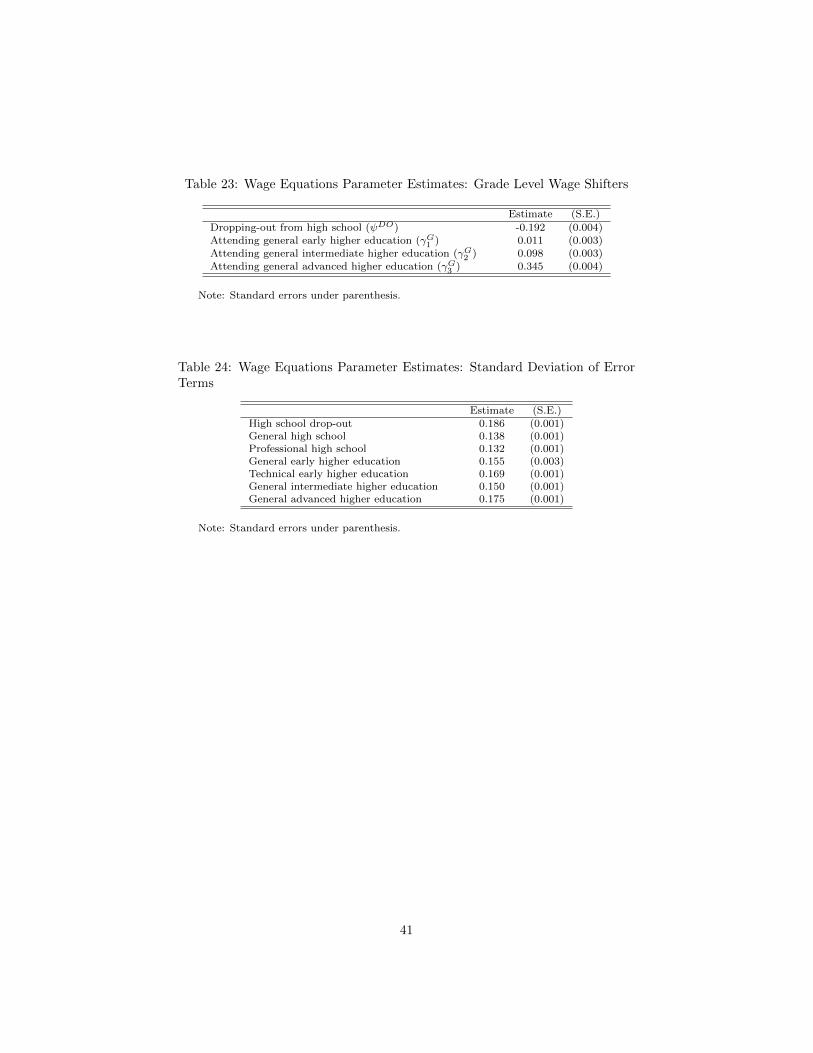
Table 23: Wage Equations Parameter Estimates: Grade Level Wage Shifters

Estimate (S.E.)

Dropping-out from high school (ψDO) -0.192 (0.004)Attending general early higher education (γG1 ) 0.011 (0.003)Attending general intermediate higher education (γG2 ) 0.098 (0.003)Attending general advanced higher education (γG3 ) 0.345 (0.004)

Note: Standard errors under parenthesis.

Table 24: Wage Equations Parameter Estimates: Standard Deviation of ErrorTerms

Estimate (S.E.)High school drop-out 0.186 (0.001)General high school 0.138 (0.001)Professional high school 0.132 (0.001)General early higher education 0.155 (0.003)Technical early higher education 0.169 (0.001)General intermediate higher education 0.150 (0.001)General advanced higher education 0.175 (0.001)

Note: Standard errors under parenthesis.

41

Tab

le25:

Un

ob

serv

edH

eter

ogen

eity

Para

met

ers

Typ

e1

Typ

e2

Typ

e3

Typ

e4

Typ

e5

Est

imate

(S.E

.)E

stim

ate

(S.E

.)E

stim

ate

(S.E

.)E

stim

ate

(S.E

.)E

stim

ate

(S.E

.)D

istr

ibu

tion

param

ete

rs

(qk)

1.4

68

(0.0

34)

-0.0

38

(0.0

33)

-0.7

36

(0.0

36)

0.8

30

(0.0

30)

--

Typ

eP

rob

ab

ilit

ies

(pk)

0.4

78

0.1

06

0.0

53

0.2

53

0.1

10

Param

ete

rs

insc

hooli

ng

con

sum

pti

on

valu

e(θ

s)

Gen

eral

sect

or

5.8

52

(0.1

23)

1.6

17

(0.0

39)

10.5

77

(0.2

47)

7.6

47

(0.1

88)

3.9

22

(0.0

64)

Pro

fess

ion

al

sect

or

2.3

10

(0.1

40)

-0.5

62

(0.1

08)

5.3

29

(0.2

36)

6.3

94

(0.3

00)

3.0

76

(0.1

92)

Tec

hn

ical

sect

or

4.9

39

(0.0

91)

1.4

58

(0.1

60)

10.0

63

(0.1

85)

6.9

36

(0.1

37)

4.8

39

(0.2

27)

Param

ete

rs

inw

ages

(ηs)

Gen

eral

sect

or

-0.2

87

(0.0

00)

-0.2

75

(0.0

00)

0.3

07

(0.0

03)

0.0

08

(0.0

02)

-0.2

13

(0.0

02)

Pro

fess

ion

al

sect

or

-0.1

93

(0.0

02)

-0.1

26

(0.0

04)

0.3

60

(0.0

05)

0.0

26

(0.0

03)

-0.2

75

(0.0

00)

Tec

hn

ical

sect

or

-0.1

54

(0.0

03)

0.1

71

(0.0

03)

-0.2

41

(0.0

01)

-0.0

26

(0.0

21)

-0.2

16

(0.0

03)

Note

:S

tan

dard

erro

rsu

nd

erp

are

nth

esis

.

42