Dichotomizing Children’s Behavior Problems:

Carving Nature at Its Joints

Sandy Braver, Jenessa Shapiro & Amy Weimer

SPRI and Quant Seminar Presentation

2

Statisticians Have Strongly Argued Against Dichotomizing Inherently

Continuous Variables (MacCallum et al., 2002)

• Very Common Practice• Derives from a “Group” ANOVA Mentality• Medical Model:Categories of Disease, Not Continua• Can Handle Through Regression Instead, But Not All

Researchers Know This• A Number of Statistical and Inferential Problems

Result

3

Statistical Problems

• “Dichotomization is rarely defensible and often will yield misleading results.”

• Lower Statistical Power• Cutpoints Are Typically Arbitrary• Other Cutpoints Might Not Replicate Result• Cutpoint Itself (e.g. median) Won’t Replicate• Forces one into nonsensical positions:

1 and 62 (both below cutpoint) are the SAME, but 62 and 63 (one below and one above cutpoint) are

DIFFERENT

4

But Real World Often Demands Dichotomization

• Selection Problems• Screening• At Risk• Insurance• DSMIV • (But see Fall 2005 Special Issue of Journal of

Abnormal Psychology, which argues for replacing categorical approach of DSMIV with a DIMENSIONAL Approach in Forthcoming DSMV)

5

Dichotomization Natural and Appropriate for Some Medical

Problems • Cancer

For Other Problematic Conditions, Dichotomization More Arbitrary•High Blood Pressure•Diabetes•Depression and Most Mental Health Conditions

• Pregnancy• Death

6

NIMH: “Congress is Interested in Us Preventing or Treating Serious Mental

Health Problems”

“I Need to Show Them We Can Prevent Schizophrenia”

Our Primary Dependent Variable at PRC: Child Well-Being or Mental Health

“Caseness” Desired By Policy-Makers; Detecting Children Who Are

Seriously Mentally ill

7

Current Standard:Child Behavior Checklist (CBCL)

Achenbach• E.g., The 2001 Annual Report to Congress on

the Evaluation of the Comprehensive Community Mental Health Services for Children and Their Families Program says:

“The CBCL (Achenbach, 1991a) has been identified as the most reliable and valid parent report measure currently available for assessing children's emotional and behavioral problems (Reitman, Hummel, Franz, & Gross, 1998).”

8

Characteristics of the CBCL• 133 items: “Argues A Lot”; “Depressed, Withdrawn”• not true=0, somewhat or sometimes true =1, very true or often

true=2• Parent Report, Youth Self-Report, Teacher Report• Total Problems Score; Broad Band (Internalizing,

Externalizing); Narrow Band (e.g., Attention Problems/Hyperactivity, Oppositional Defiant, and Somatization)

• Raw Score, T-Score• Clinical Cutoff: “Internalizing, Externalizing, and Total

Problems scale T-scores are considered in the clinical range if they are above 63, while scores from 60 to 63 are borderline. Scores in the clinical range indicate a need for clinical care.”

• High Reliability (Alpha and Test-Retest)• Excellent National Norms• Lots of Validation Studies• Thousands of studies use the CBCL and report the percent of

their study group in the clinical (and borderline clinical) range, reifying the arbitrary clinical range cutoff

9

Alternatives to the CBCL

• Rutter• DISC (Takes several hours to administer,

many hours to train and certify testors, matches Psychiatrists’ DSM Diagnosis)

• Short Form of CBCL, the Behavior Problem Index (BPI) 32 items

• Not Copyrighted—Free• We Use BPI

10

Validation Studies Need a Criterion

• CBCL’s Criterion is referred to as “Referral Status”

• That is, A Clinic Sample vs A “Matched” Non-Clinic Sample Were Assessed

• Lots of differences are found between the two “status groups” on various CBCL variables, which establishes validity of scale

11

Cutoff Determination ALSO requires a criterion variable

• Choice of Cutoff Value for Caseness Determination can and should use the same criterion variable as for Validity studies

• This is a very common problem in medical settings (e.g., high blood pressure, diabetes) and human resources settings (e.g., hire, no hire)

• a technology (ROC) for distinguishing “normal” from “case” has developed and received acceptance

12

Brief Primer on Cutoff Determination:ROC (Receiver Operating Characteristic,

Signal Detection) Analysis

Diagnosis

- +

Tests’ Value Relative to Proposed Cutoff

Below False

Negative(FN)

At or Above

False Positive(PN)

13

ROC Analysis Uses Constructs of Sensitivity & Specificity

• SE: {Sensitivity}: Is the proposed cutoff value sensitive? Does it detect most of the Positive Cases?

• SP: {Specificity}: Is the proposed cutoff value specific to the positive cases? Does it correctly indicate the cases that are NOT POSITIVE

• For a good test, with a well selected cutoff, both should be very high.

14

Sensitivity & Specificity ExampleDiagnosis

- +Test’s Value Relative to Proposed Cutoff

Below A=500 B=200 A+B=700

At or Above

C=100 D=200 C+D=300

A+C=600 B+D=400 T=1000

=A+B+C+D50.

400DB

200D

SE=Sensitivity=Prob of pos test given pos diag=

833.600CA

500A

SP=Specificity= Prob of neg test given neg diag=

1-Specificity= Prob of POS test given neg diag=.167

1-Specificity Should be LOW

15

Ideal pointCoordinates of the Curve

Test Result Variable(s): educ Educational Level (years)

7.00 1.000 1.000

10.00 .911 .861

13.00 .671 .269

14.50 .647 .269

15.50 .326 .116

16.50 .190 .005

17.50 .151 .000

18.50 .116 .000

19.50 .012 .000

20.50 .004 .000

22.00 .000 .000

Positive ifGreater Thanor Equal To

aSensitivity 1 - Specificity

The test result variable(s): educ Educational Level (years)has at least one tie between the positive actual state groupand the negative actual state group.

The smallest cutoff value is the minimumobserved test value minus 1, and the largest cutoffvalue is the maximum observed test value plus 1.All the other cutoff values are the averages of twoconsecutive ordered observed test values.

a.

Best Cutoff

1-SP too high

SE too low

ROC Graph (SPSS):Sensitivity & 1-Specificity Are Calculated

Repeatedly, for Each Potential Cutoff Value

A CONVINCING Cutoff Should Be Noticeably Better Than Its Neighbors

Potential Cutoffs

15

16

A CONVINCING Cutoff Should Be Noticeably Better Than Its Neighbors• Otherwise, Cutoff Is Arbitrary

• Flat ROC Curves Provide No Compelling Rationale For Choosing One Cutoff Value vs Another For This Important Real World Choice

• Depends on Emphasis on SE or SP

Alternatives to Sensitivity & Specificity (Helena Kraemer)

Diagnosis

- +

Test’s Value Relative to Proposed Cutoff

Below A=500 B=200 A+B=700

At or Above

C=100 D=200 C+D=300

A+C=600 B+D=400 T=1000=A+B+C+D

PVP=predictive value of a positive test =(D=200)/((C+D=300) =.67PVN=predictive value of a negative test =(A=500)/((A+B=700)=.71

Quality PVP=κ(0,0)=(PVP-P)/(1-P)=(.67-.4)/(1-.4)=.44, weights avoiding False PositivesP=Prevalence (of a Pos Diag) =(B+D=400)/(T=1000)=.40

Quality PVN=κ(1,0)=(PNP-(1-P))/P=(.71-.6)/.4=.29,weights avoiding False NegativesCohen’s Kappa [κ(.5,0)]=.35, weights FN & FP equally

Weighted Kappa [κ(r,0)] [e.g. κ(.8,0)]=.31, weights FN & FP relatively, by r

Efficiency=EFF=Overall Prob of Correct Class=(A+D=500+200=700)/(T=1000)=.70

PHI coefficient (Φ)

r =WFN/(WFN+WFP), W is weight; r of .8 means that FN are 4 times worse than FP 4/(4+1)

17

http://www.erlbaum.com/Documents/JPA/3_04/2%20x%202%20Stat%20Calculator.xls

Diagnosis Present Diagnosis AbsentTest Positive 118 52 170

Test Negative 69 761 830187 813 1000

Prevalence 0.187 Prevalence* Enter #(*Enter prevalence as a value between 0 and 1)

Sensitivity 0.631 SensitivitySpecificity 0.936 Specificity

Odds ratio (OR) 25.027 Odds ratio (OR)Likelihood Ratio+ (LR+) 9.866 Likelihood Ratio+ (LR+)

Likelihood Ratio- (LR-) 2.537 Likelihood Ratio- (LR-)

Positive Predictive Power (PPP) 0.694 Positive Predictive Power (PPP)Negative Predictive Power (NPP) 0.917 Negative Predictive Power (NPP)

Overall Correct Classification (OCC) 0.879 Overall Correct Classification (OCC)Incremental PPP 0.507 Incremental PPPIncremental NPP 0.104 Incremental NPP

Quality PPP 0.624 Quality PPPQuality NPP 0.555 Quality NPP

Kappa 0.588 KappaKraemer's Kappa 0.594 Kraemer's Kappa

Phi coefficient 0.589 Phi coefficientPretest Odds+ 0.230 Pretest Odds+

Posttest Odds+ 2.269 Posttest Odds+Pretest Odds- 4.348 Pretest Odds-

Posttest Odds- 11.029 Posttest Odds-

Dx Present Dx AbsentTest Positive

Test Negative

**Program created by Jared DeFife, Adelphi University, 2004.

*Formulas and calculations based on Streiner, D.L. (2003). Diagnosing tests: Using and misusing diagnostic and screening tests. Journal of Personality Assessment, 81(3), 209-219.

DIAGNOSTIC EFFICIENCY STATISTICS CALCULATOR*

For statistics based upon the observed prevalence rate from your SAMPLE, use the results below:

To customize a prevalence rate that is based on a POPULATION (I.e. not from your sample),

enter a prevalence rate below then calculate by

click ing on the YELLOW BOX :

**ALWAYS CLICK HERE TO CALCULATE FINAL RESULTS**

Enter raw data into RED cells then click the YELLOW box to calculate:

Population Prevalence Adjusted Table:

18

19

Example 1

0

0.2

0.4

0.6

0.8

1

0 0.2 0.4 0.6 0.8 1

k(0,0) Qual PVP

k(1,

0) Q

ual

PV

N

3

4

2

sens & spec

0

0.2

0.4

0.6

0.8

1

0 0.1 0.2 0.3 0.4 0.5 0.6 0.7 0.8 0.9 1

1 - spec

sen

s

6

5

4

3

2

Raw Data Example 1

0

0.2

0.4

0.6

0.8

1

1 2 3 4 5 6 7 8

scoreP

rob

of

crit

weighted kappas and phi

0

0.1

0.2

0.3

0.4

0.5

1 2 3 4 5 6 7

score

κ(.2,0) κ(.4,0) κ(.5,0)=Cohen's κ(.6,0) κ(.8,0) phi

rpbi Note that it’s>Φ

20

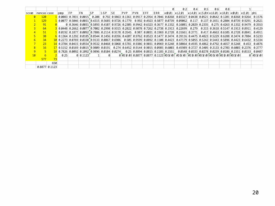
0 0.2 0.4 0.5 0.6 0.8 1score noncasecase prop FP FN SP 1-SP SE PVP PVN EFF ERR κ(0,0) κ(.2,0) κ(.4,0) κ(.5,0)=Cohen'sκ(.6,0) κ(.8,0) κ(0,0) κ(1,0) phi

0 120 1 0.0083 0.7031 0.0015 0.208 0.792 0.9863 0.1361 0.9917 0.2954 0.7046 0.0268 0.03327 0.0438 0.0521 0.0642 0.1201 0.0268 0.9264 0.15761 129 1 0.0077 0.5046 0.0031 0.4315 0.5685 0.9726 0.1779 0.992 0.4923 0.5077 0.0739 0.09062 0.117 0.137 0.1651 0.2804 0.0739 0.9291 0.26212 91 0 0 0.3646 0.0031 0.5893 0.4107 0.9726 0.2305 0.9942 0.6323 0.3677 0.1332 0.16081 0.2029 0.2335 0.275 0.4263 0.1332 0.9479 0.35533 64 3 0.0448 0.2662 0.0077 0.7002 0.2998 0.9315 0.2822 0.9878 0.7262 0.2738 0.1913 0.22699 0.279 0.315 0.3618 0.5147 0.1913 0.8911 0.41294 51 1 0.0192 0.1877 0.0092 0.7886 0.2114 0.9178 0.3545 0.987 0.8031 0.1969 0.2728 0.31661 0.3771 0.417 0.4663 0.6105 0.2728 0.8841 0.49115 38 6 0.1364 0.1292 0.0185 0.8544 0.1456 0.8356 0.4207 0.9762 0.8523 0.1477 0.3474 0.39116 0.4475 0.4823 0.5229 0.6288 0.3474 0.7884 0.52336 34 10 0.2273 0.0769 0.0338 0.9133 0.0867 0.6986 0.505 0.9599 0.8892 0.1108 0.4423 0.47179 0.5055 0.5242 0.5443 0.5896 0.4423 0.6432 0.53347 23 14 0.3784 0.0415 0.0554 0.9532 0.0468 0.5068 0.5781 0.9386 0.9031 0.0969 0.5248 0.50864 0.4935 0.4862 0.4792 0.4657 0.5248 0.453 0.48768 16 17 0.5152 0.0169 0.0815 0.9809 0.0191 0.274 0.6452 0.9144 0.9015 0.0985 0.6003 0.45989 0.3727 0.3405 0.3133 0.2703 0.6003 0.2376 0.37779 5 18 0.7826 0.0092 0.1092 0.9896 0.0104 0.0274 0.25 0.8894 0.8815 0.1185 0.1551 0.0548 0.0333 0.0278 0.0239 0.0186 0.1551 0.0153 0.0487

10 6 2 0.25 0 0.1123 1 0 0 #DIV/0! 0.8877 0.8877 0.1123 #DIV/0! #DIV/0! #DIV/0! #DIV/0! #DIV/0! #DIV/0! #DIV/0! 0 #DIV/0!577 73

6500.8877 0.1123

21

Example 2

0

0.2

0.4

0.6

0.8

1

0 0.1 0.2 0.3 0.4 0.5 0.6

k(0,0) Qual PVP

k(1,

0) Q

ual

PV

N

3

4

2

sens & spec

0

0.2

0.4

0.6

0.8

1

0 0.1 0.2 0.3 0.4 0.5 0.6 0.7 0.8 0.9 1

1 - spec

sen

s

6

5

4

3

2

Raw Data Example 1

0

0.2

0.4

0.6

0.8

1 2 3 4 5 6 7 8

score

Pro

b o

f cr

it

weighted kappas and phi

0

0.1

0.2

0.3

0.4

0.5

0.6

0.7

1 2 3 4 5 6 7

score

κ(.2,0) κ(.4,0) κ(.5,0)=Cohen's κ(.6,0) κ(.8,0) phi

rpbi

Φ>rpbi

22

Example 3

0

0.2

0.4

0.6

0.8

1

0 0.05 0.1 0.15 0.2 0.25 0.3 0.35 0.4 0.45

k(0,0) Qual PVP

k(1,

0) Q

ual

PV

N

3 42

sens & spec

0

0.2

0.4

0.6

0.8

1

0 0.1 0.2 0.3 0.4 0.5 0.6 0.7 0.8 0.9 1

1 - spec

sen

s

6

5

4

3

2

weighted kappas and phi

0

0.1

0.2

0.3

0.4

0.5

1 2 3 4 5 6 7

score

κ(.2,0) κ(.4,0) κ(.5,0)=Cohen's κ(.6,0) κ(.8,0) phi

Raw Data Example 3

0

0.2

0.4

0.6

1 2 3 4 5 6 7 8

score

Pro

b o

f cr

it

rpbi

Φsubstantially>rpbi

23

Example 4

0

0.1

0.2

0.3

0 0.1 0.2 0.3 0.4 0.5

k(0,0) Qual PVP

k(1,

0) Q

ual

PV

N

3 42 5 6

sens & spec

0

0.2

0.4

0.6

0.8

1

0 0.1 0.2 0.3 0.4 0.5 0.6 0.7 0.8 0.9 1

1 - spec

sen

s

6

5

4

3

2

weighted kappas and phi

0

0.1

0.2

0.3

0.4

1 2 3 4 5 6 7

score

κ(.2,0) κ(.4,0) κ(.5,0)=Cohen's κ(.6,0) κ(.8,0) phi

rpbi

Φsubstantially>rpbi

Raw Data Example 4

0

0.2

0.4

0.6

1 2 3 4 5 6 7 8

score

Pro

b o

f cr

it

24

Only A Peaked ROC Curve Provides Strong Rationale for A Specific Value For

Cutoff, Whatever the Index Chosen• Chooses Same Cutoff By Any Criterion• No Need to Defend Choice of SE & SP, vs PVP

& PVN, vs Quality version, vs Kappas• No Need to Defend Weights for FN vs FP in

Kappas• No Need to Know Prevalence• A Peaked ROC curve will result only if the raw

data has a “Joint”, • Joint on all curves at same point• Want to “carve” (choose as cutoff) right at

Nature’s joint

25

Applying ROC Concepts to CBCL• Needs a True Dichotomous Criterion• i.e., the “Diagnosis”• Achenbach Uses Referral Status, the Same Variable Used as

Criterion in Validity Studies, As Recommended• Referred vs Not Referred • i.e., Clinic Cases vs Normal• The cutoff of 63 (Clinical Range) was chosen by Achenbach in order

to meet the following Criterion: Minimizing Error (=ERR=FN+FP=1-Efficiency)

• (i.e., Maximize EFF)• Difficulties with this Approach:

Doesn’t Provide ROC Curves, so Can’t Determine Whether ROC is Peaked, Whether that Cutoff Is Noticeably Better Than Neighbors

Is Equal Weighting of FN & FP Appropriate For Caseness?

26

Our Biggest Issue with the CBCL: The Validity Criterion Chosen

• They Say It’s “Referred vs Non-Referred”, But It’s Really Not

• It’s Really Clinic vs Non-Clinic• Not Known WHO Referred Or If “Referred” By Anyone At

All• This Leads to the Question of Which Kids Get to Clinic• Empirical Research on Parents Taking Kids to Clinic

Shows Many Factors Are Influential, Only One of Which is Kid’s Mental State (Lobitz and Johnson, 1975)Parents’ LabelingParent’s Belief in Efficacy of Clinical Therapy Insurance IssuesParent’s (Mother’s) Own Clinical Levels

27

Their Method Prevents Estimation of Prevalence, Needed For Some Indexes

• What Is prevalence of serious mental illness in Adolescents?

• Major Review Article of 52 Studies (Roberts,1998)• Lots Of Issues• What’s Criterion, What’s Population?• 3 to 54%• Median: About 15%• This “Feels About Right” to Diagnosticians• Matches Prevalence of Other Mental Health

Problems• CBCL Clinical Range T Score of 63 = About 15%

28

Is There Another Easy To Use True Dichotomous Criterion? Our Idea

• Teacher Report of Referral

• Actual Referral, Not Whether Being Seen

• Matches Notions About NEED For Services, Rather Than Use Of Services

• Teachers Are More Neutral Than Parents

• Teachers Have Better Frame Of Reference For Disturbed Behavior

29

Alternative: Peer Report of Psychopathology

• Data Suggests Peers of Adolescents Are Excellent Judges of Pathology

• Sociometrics Ratings of Peers Predict Better Than Any Other Variable Later Problem Behavior

• Sociometrics Cumbersome to Acquire

• Teachers Good Detectors of Sociometric Data

• Teacher Report on Peers Proxy for Peer Report

30

PAYS Data Set

• About 400 families• All with 7th Graders• Recruited from schools in AZ and

Riverside, CA• Will be 3 Waves• Mother, Father, Child Report on BPI

Internalizing and Externalizing• 2 Teacher Reports on our adapted version

of BPI

31

* p < .001

Correlations of Teacher 1, Teacher 2, Child, Mom and Dad on BPI

1 2 3 4 5

1. Teacher 1 .57* .33* .26* .32*

2. Teacher 2 .39* .30* .39*

3. Child's CBCL .35* .28*

4. BPI (Mom) .47*

5. BPI (Dad)        

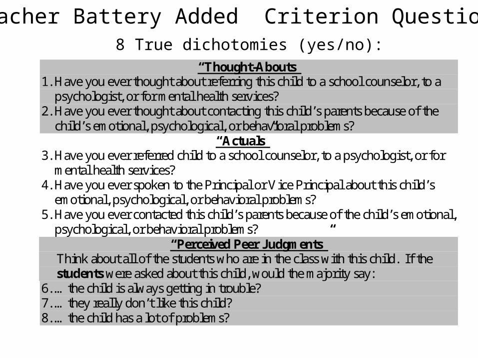
8 True dichotomies (yes/no):

Teacher Battery Added Criterion Questions

“Thought-Abouts” 1. Have you ever thought about referring this child to a school counselor, to a

psychologist, or for mental health services? 2. Have you ever thought about contacting this child’s parents because of the

child’s emotional, psychological, or behavioral problems? “Actuals”

3. Have you ever referred child to a school counselor, to a psychologist, or for mental health services?

4. Have you ever spoken to the Principal or Vice Principal about this child’s emotional, psychological, or behavioral problems?

5. Have you ever contacted this child’s parents because of the child’s emotional, psychological, or behavioral problems?

“Perceived Peer Judgments” Think about all of the students who are in the class with this child. If the students were asked about this child, would the majority say: 6. …the child is always getting in trouble? 7. …they really don’t like this child? 8. …the child has a lot of problems?

33

2 3 4 5 6 7 8 T1-T2 cor % yes

Has teacher ever thought about:1. Contacting this child's parents because of the child's emotional, psychological, or .52* .41* .77* .43* .51* .37* .49* .37* 17.9

2. Referring this child to a school counselor, to a psychologist, or for mental health services? .44* .47* .68* .46* .34* .56* .13* 9.5

Has teacher ever :3. Spoken to Principal or Vice Principal about this child's emotional, psychological, or behavior problems? .45* .46* .43* .33* .42* .19* 5.8

4. Contacted this child's parents because of the child's emotional, psychological, or behavior problems? .41* .51* .36* .48* .36* 13.9

5. Referred this child to a school counselor, to a psychologist, or for mental health services? .32* .28* .45* .14* 5.2

Would majority of kids in child's class say:

6. Child always is getting into trouble? .44* .55* .42* 8.4

7. They really don't like this child? .68* .04 4.0

8. This child has a lot of problems? .21* 5.2

Correlations of 8 dichotomous items; Percent of Teachers that said “Yes” for each item

* p<.05

34

Teacher BPI % yesHas teacher ever thought about:

1. Contacting this child's parents because of the child's emotional, psychological, or behavior problems? .56* 17.92. Referring this child to a school counselor, to a psychologist, or for mental health services? .42* 9.5Has teacher ever :3. Spoken to Principal or Vice Principal about this child's emotional, psychological, or behavior problems? .31* 5.84. Contacted this child's parents because of the child's emotional, psychological, or behavior problems? .49* 13.95. Referred this child to a school counselor, to a psychologist, or for mental health services? .33* 5.2Would majority of kids in child's class say:

6. Child always is getting into trouble? .49* 8.47. They really don't like this child? .29* 4.08. This child has a lot of problems? .37* 5.2

Correlations between individual dichotomies (N=700)with teacher BPI

* p<.001

35

Teacher Thought About Contacting Parentssens & spec

0

0.2

0.4

0.6

0.8

1

0 0.1 0.2 0.3 0.4 0.5 0.6 0.7 0.8 0.9

1 - spec

sen

s

6

5

43

2

7

0

0.2

0.4

0.6

0.8

1

0 0.1 0.2 0.3 0.4 0.5 0.6 0.7 0.8 0.9

k(0,0) Qual PVP

k(1,

0) Q

ual

PV

N

3

4

2

5

6

8

7

weighted kappas and phi

0

0.1

0.2

0.3

0.4

0.5

0.6

0.7

0 1 2 3 4 5 6 7 8 9 10

score

κ(.2,0) κ(.4,0) κ(.5,0)=Cohen's κ(.6,0) κ(.8,0) phi

rpbi

0

0.1

0.2

0.3

0.4

0.5

0.6

0.7

0.8

0.9

1

1 2 3 4 5 6 7 8 9 10 11

score

pro

po

rtio

n c

ases

36

Teacher Actually Contacted Parentssens & spec

0

0.2

0.4

0.6

0.8

1

0 0.1 0.2 0.3 0.4 0.5 0.6 0.7 0.8 0.9

1 - spec

sen

s

6

5 4

32

7

0

0.2

0.4

0.6

0.8

1

0 0.1 0.2 0.3 0.4 0.5 0.6

k(0,0) Qual PVP

k(1,

0) Q

ual

PV

N

3

4

2

5

6

8

7

weighted kappas and phi

0

0.1

0.2

0.3

0.4

0.5

0.6

0 1 2 3 4 5 6 7 8 9 10

score

κ(.2,0) κ(.4,0) κ(.5,0)=Cohen's κ(.6,0) κ(.8,0) phi

rpbi

0

0.1

0.2

0.3

0.4

0.5

0.6

0.7

0.8

0.9

1

1 2 3 4 5 6 7 8 9 10 11

score

pro

po

rtio

n c

ases

Better, but still no real joint

37

thought actual peerTeacher

BPI % Yesthought 1 0.77* 0.58* 0.58* 19.8

actual 1 0.57* 0.54* 16.1

peer 1 0.52* 10.8

Teacher BPI 1

Combine Dichotomies: 1 if ANY, 0 if NONE

38

Thought Aboutssens & spec

0

0.2

0.4

0.6

0.8

1

0 0.1 0.2 0.3 0.4 0.5 0.6 0.7 0.8 0.9

1 - spec

sen

s

6

5

4

3 2

7

0

0.1

0.2

0.3

0.4

0.5

0.6

0.7

0.8

0.9

1

1 2 3 4 5 6 7 8 9 10 11

score

pro

po

rtio

n c

ases

0

0.2

0.4

0.6

0.8

1

0 0.1 0.2 0.3 0.4 0.5 0.6 0.7 0.8 0.9

k(0,0) Qual PVP

k(1,

0) Q

ual

PV

N

3

4

2

5

6

8

7

weighted kappas and phi

0

0.1

0.2

0.3

0.4

0.5

0.6

0.7

0 1 2 3 4 5 6 7 8 9 10

score

κ(.2,0) κ(.4,0) κ(.5,0)=Cohen's κ(.6,0) κ(.8,0) phi

rpbi

39

Actualssens & spec

0

0.2

0.4

0.6

0.8

1

0 0.1 0.2 0.3 0.4 0.5 0.6 0.7 0.8 0.9

1 - spec

sen

s

6

5

4 32

7

0

0.2

0.4

0.6

0.8

1

0 0.1 0.2 0.3 0.4 0.5 0.6 0.7 0.8

k(0,0) Qual PVP

k(1,

0) Q

ual

PV

N

3

4

2

5

6

8

7

weighted kappas and phi

0

0.1

0.2

0.3

0.4

0.5

0.6

0.7

0 1 2 3 4 5 6 7 8 9 10

score

κ(.2,0) κ(.4,0) κ(.5,0)=Cohen's κ(.6,0) κ(.8,0) phi

rpbi

0

0.1

0.2

0.3

0.4

0.5

0.6

0.7

0.8

0.9

1

1 2 3 4 5 6 7 8 9 10 11

score

pro

po

rtio

n c

ases

40

Peerssens & spec

0

0.2

0.4

0.6

0.8

1

0 0.1 0.2 0.3 0.4 0.5 0.6 0.7 0.8 0.9

1 - spec

sen

s

6 5 43 2

7

weighted kappas and phi

0

0.1

0.2

0.3

0.4

0.5

0.6

0.7

0 1 2 3 4 5 6 7 8 9 10

score

κ(.2,0) κ(.4,0) κ(.5,0)=Cohen's κ(.6,0) κ(.8,0) phi

rpbi

0

0.2

0.4

0.6

0.8

1

0 0.1 0.2 0.3 0.4 0.5 0.6 0.7

k(0,0) Qual PVP

k(1,

0) Q

ual

PV

N

34

2

5

6

8

7

0

0.1

0.2

0.3

0.4

0.5

0.6

0.7

0.8

0.9

1

1 2 3 4 5 6 7 8 9 10 11

score

pro

po

rtio

n c

ases

Nature at the Joint?

41

So, pick a score of 6 on BPI as Cutpoint with Peers as Criterion

SP .91

1-SP .09

SE .70

PVP .50

PVN .96

EFF .89

ERR .11

κ(0,0) .44

κ(.2,0) .47

κ(.4,0) .51

κ(.5,0)=Cohen's .52

κ(.6,0) .54

κ(.8,0) .59

κ(1,0) .64

phi .53

But why not just ask teacher the dichotomous

questions:

Forget the BPI