Diagnosing atmosphere-ocean general circulation model errors

relevant to the terrestrial biosphere using the Koppen

climate classification

Anand Gnanadesikan1 and Ronald J. Stouffer1

Received 6 September 2006; revised 12 October 2006; accepted 18 October 2006; published 16 November 2006.

[1] Coupled atmosphere-ocean-land-sea ice climatemodels (AOGCMs) are often tuned using physicalvariables like temperature and precipitation with the goalof minimizing properties such as the root-mean-squareerror. As the community moves towards modeling the earthsystem, it is important to note that not all biases haveequivalent impacts on biology. Bioclimatic classificationsystems provide means of filtering model errors so as tobring out those impacts that may be particularly importantfor the terrestrial biosphere. We examine one suchdiagnostic, the classic system of Koppen, and show that itcan provide an ‘‘early warning’’ of which model biases arelikely to produce serious biases in the land biosphere.Moreover, it provides a rough evaluation criterion for theperformance of dynamic vegetation models. State-of-the artAOGCMs fail to capture the correct Koppen zone in about20–30% of the land area excluding Antarctica, andmisassign a similar fraction to the wrong subzone.Citation: Gnanadesikan, A., and R. J. Stouffer (2006),

Diagnosing atmosphere-ocean general circulation model errors

relevant to the terrestrial biosphere using the Koppen climate

classification, Geophys. Res. Lett., 33, L22701, doi:10.1029/

2006GL028098.

1. Introduction

[2] The process of developing climate models involves avast array of choices. Numerical schemes, parameterizationsof subgrid-scale processes, parameter values within theseparameterizations- a host of issues face any model devel-opment team. The recent process of model development forthe Intergovernmental Panel on Climate Change (IPCC)Fourth Assessment Report (AR4) at the Geophysical FluidDynamics Lab (GFDL) involved both qualitative metrics(e.g. maintenance of a reasonable thermohaline overturningand El Nino) and quantitative metrics (e.g. minimization ofthe maximum error and RMS error in sea surface temper-ature, minimization of the near-surface air temperature andprecipitation errors). An implicit assumption for many suchmetrics, however, is that biases in temperature and precip-itation are weighted equally regardless of location. Forexample, a 0.3 m/yr underprediction in precipitation in theAmazon rainforest (where the mean precipitation is high) isweighted the same as a 0.3 m/yr underprediction in themiddle of North America (which could flip a region fromgrassland to desert).

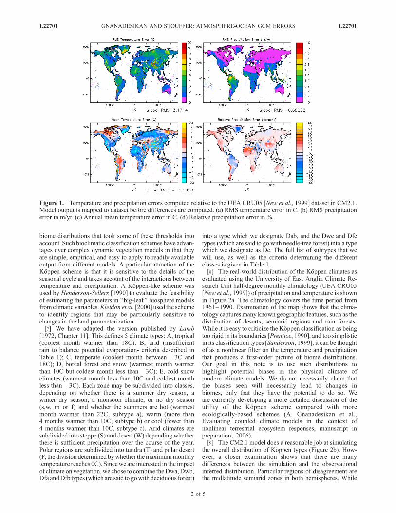
[3] From the point of view of physical climate, this is avery defensible approach. It protects modelers from beingaccused of tuning the ‘‘skill score’’ of their particular modelso as to maximize the good points of that model. However,as we will demonstrate in this note, not all model errors areequivalent in how they impact biology. There is evidencethat the terrestrial biosphere is affected by key thresholdswhich must be properly simulated in order for models to beable to simulate the present-day biosphere and to be crediblein simulating its future evolution. This demands that devel-opers of coupled models consider not only the raw physicalfields such as temperature and precipitation, but additionaldiagnostics which are sensitive to the impact of these fieldson biospherically relevant processes.[4] An illustration of how models are evaluated from a

physical point of view is shown in Figure 1, which showssurface temperatures and precipitation over land in a sim-ulation using the CM2.1 global coupled climate model[Delworth et al., 2006] recently developed at GFDL. Thismodel consists of ocean, sea ice, and atmosphere models,with a land model based on that of Milly and Shmakin[2002] that does not include vegetative feedback. Exami-nation of the mean and RMS precipitation errors (Figure 1)shows that there are large errors over the tropical regions,particularly the Amazon, and smaller errors over the tem-perate midlatitudes. Large temperature errors are also seenover the Sahara. At the edges of mountainous areas (par-ticularly the Tibetan plateau), smoothing of topographywithin the model leads to significant errors in temperature.The percentage precipitation errors are largest over theSahara, where precipitation rates are low, and in mountain-ous regions.[5] Different errors, however, will not have equivalent

impacts when considered from the point of view of indi-vidual organisms. An example of this that is familiar toevery gardener is the ability of plants to survive coldwinters. A 2C cold bias may well mean that a particularplant is unable to survive a winter, while a 2C warm biasmay have little effect. Similarly, vegetation may be verysensitive to whether or not the ground dries out during thesummer. This paper examines these effects using a classicbioclimatic model, proposed originally by the climatologistW. Koppen. We show that the distribution of Koppenclimate types within models provides a way of isolatingerrors that can be important for land biology, thus providingguidance for developers of physical climate models.

2. Koppen Climate Index

[6] During the first part of the 20th century, the clima-tologist W. Koppen developed a scheme for predicting

GEOPHYSICAL RESEARCH LETTERS, VOL. 33, L22701, doi:10.1029/2006GL028098, 2006ClickHere

for

FullArticle

1NOAA Geophysical Fluid Dynamics Laboratory, Princeton, NewJersey, USA.

This paper is not subject to U.S. copyright.Published in 2006 by the American Geophysical Union.

L22701 1 of 5

biome distributions that took some of these thresholds intoaccount. Such bioclimatic classification schemes have advan-tages over complex dynamic vegetation models in that theyare simple, empirical, and easy to apply to readily availableoutput from different models. A particular attraction of theKoppen scheme is that it is sensitive to the details of theseasonal cycle and takes account of the interactions betweentemperature and precipitation. A Koppen-like scheme wasused by Henderson-Sellers [1990] to evaluate the feasibilityof estimating the parameters in ‘‘big-leaf’’ biosphere modelsfrom climatic variables.Kleidon et al. [2000] used the schemeto identify regions that may be particularly sensitive tochanges in the land parameterization.[7] We have adapted the version published by Lamb

[1972, Chapter 11]. This defines 5 climate types: A, tropical(coolest month warmer than 18C); B, arid (insufficientrain to balance potential evaporation- criteria described inTable 1); C, temperate (coolest month between �3C and18C); D, boreal forest and snow (warmest month warmerthan 10C but coldest month less than �3C); E, cold snowclimates (warmest month less than 10C and coldest monthless than �3C). Each zone may be subdivided into classes,depending on whether there is a summer dry season, awinter dry season, a monsoon climate, or no dry season(s,w, m or f) and whether the summers are hot (warmestmonth warmer than 22C, subtype a), warm (more than4 months warmer than 10C, subtype b) or cool (fewer than4 months warmer than 10C, subtype c). Arid climates aresubdivided into steppe (S) and desert (W) depending whetherthere is sufficient precipitation over the course of the year.Polar regions are subdivided into tundra (T) and polar desert(F, the division determined bywhether themaximummonthlytemperature reaches 0C). Sincewe are interested in the impactof climate on vegetation, we chose to combine theDwa, Dwb,Dfa andDfb types (which are said to gowith deciduous forest)

into a type which we designate Dab, and the Dwc and Dfctypes (which are said to go with needle-tree forest) into a typewhich we designate as Dc. The full list of subtypes that wewill use, as well as the criteria determining the differentclasses is given in Table 1.[8] The real-world distribution of the Koppen climates as

evaluated using the University of East Anglia Climate Re-search Unit half-degree monthly climatology (UEA CRU05[New et al., 1999]) of precipitation and temperature is shownin Figure 2a. The climatology covers the time period from1961–1990. Examination of the map shows that the clima-tology captures many known geographic features, such as thedistribution of deserts, semiarid regions and rain forests.While it is easy to criticize the Koppen classification as beingtoo rigid in its boundaries [Prentice, 1990], and too simplisticin its classification types [Sanderson, 1999], it can be thoughtof as a nonlinear filter on the temperature and precipitationthat produces a first-order picture of biome distributions.Our goal in this note is to use such distributions tohighlight potential biases in the physical climate ofmodern climate models. We do not necessarily claim thatthe biases seen will necessarily lead to changes inbiomes, only that they have the potential to do so. Weare currently developing a more detailed discussion of theutility of the Koppen scheme compared with moreecologically-based schemes (A. Gnanadesikan et al.,Evaluating coupled climate models in the context ofnonlinear terrestrial ecosystem responses, manuscript inpreparation, 2006).[9] The CM2.1 model does a reasonable job at simulating

the overall distribution of Koppen types (Figure 2b). How-ever, a closer examination shows that there are manydifferences between the simulation and the observationalinferred distribution. Particular regions of disagreement arethe midlatitude semiarid zones in both hemispheres. While

Figure 1. Temperature and precipitation errors computed relative to the UEA CRU05 [New et al., 1999] dataset in CM2.1.Model output is mapped to dataset before differences are computed. (a) RMS temperature error in C. (b) RMS precipitationerror in m/yr. (c) Annual mean temperature error in C. (d) Relative precipitation error in %.

L22701 GNANADESIKAN AND STOUFFER: ATMOSPHERE-OCEAN GCM ERRORS L22701

2 of 5

the model does, for example, reproduce the Namib andAtacama deserts, it does not capture the Argentinian Pam-pas, the Kalahari, the Central Asian steppes or the rainshadow of the Rockies. In fact, (Figure 2c) 45.2 Mkm2 ofthe land surface is classified in the wrong type, or 30.8% ofthe land area excluding Antarctica. Moreover, 38.0 Mkm2

(25.9%) is in the wrong subtype (Figure 2d), with aparticularly significant region being the Amazonian rainforest. In total over half of the land outside Antarctica isclassified in the wrong Koppen type or subtype (using thelist in Table 1). Some of the regions (such as the Amazon)are subject to large precipitation and temperature errors.

Table 1. Koppen Vegetation Types Used in This Paper With Nominal Vegetation Typesa

Type Name (Nominal Vegetation Types) Criteria

1. Af Tropical wet (Tropical evergreen rain forest) Tmin > 18C, not BS or BW, Pmin > 62. Am Tropical moist (Tropical evergreen rain forest) Tmin > 18C, not BS or BW,

6 > Pmin > (250 � Pyear)/253. Aw Tropical Dry (Savanna/Woodland) Tmin > 18C, not BS or BW,

6, (250 � Pyear)/25 > Pmin

4. BS Semiarid (Bush to grassland) 2(Tave + Poff) > Pyear > (Tave + Poff)Poff = 0, > 30% of rain in winterPoff = 7, no wet seasonPoff = 14, > 30% of rain in summer

5. BW Desert (waste to cactus/seasonal vegetation) (Tave + Poff) > Pyear6. Cs Temperate winter wet

(Evergreen broad-leaf forest)18C > Tmin > �3C, not BS or BW,Pmax > 3Pmin, winter max., summer min.

7. Cfa Hot temperate moist (Broad-leaf forest) 18C > Tmin > �3C, not BS or BW,Not Cs or Cw, Tmax > 22C

8. Cfb Warm temperate moist (Broad-leaf forest) 18C > Tmin > �3C, not BS or BW,Not Cs or Cw, Tmax < 22C.4+ months warmer than 10C.

9. Cfc Cool temperate moist (Needle-tree forest) 18C > Tmin > �3C, not BS or BW,Not Cs or Cw, Tmax < 22C.Less than 4 months warmer than 10C.

10. Cw Temperate summer wet (Evergreen forest) 18C > Tmin > �3C, not BS or BW,Pmax > 10Pmin, summer max., winter min.

11. Dab: Cold winters/warm summers (deciduous forest) Tmax > 10C, �3C > Tmin, not BS or BW4+ months warmer than 10C.

12. Dc: Cold winters/cool summers (evergreen forest) �3C > Tmin, not BS or BW4+ months warmer than 10C.

13. Et: Tundra (tundra, dwarf trees, mosses) 10C > Tmax > 0C, Tmin < �3C14. Ef Polar desert (permanent ice or rock, little plant life) Tmax < 0C

aAs discussed by Prentice [1990], actual vegetation may differ. Tmin,max,ave are the minimum monthly, maximum monthly,and annual-average temperature in C. Pmin,max,year are the minimum monthly, maximum monthly, and annually-integratedprecipitation in cm.

Figure 2. Biases in the climate model revealed using the Koppen scheme. (a) Koppen types from data. (b) Koppen typesin CM2.1. (c) Regions (data) misidentified in CM2.1 by type. (d) Regions (data) misidentified in CM2.1 by subtype.

L22701 GNANADESIKAN AND STOUFFER: ATMOSPHERE-OCEAN GCM ERRORS L22701

3 of 5

However, in other regions (such as steppes of central Asia)the errors are less obvious.[10] It is interesting to compare the distributions of errors

across 10 models submitted to the IPCC AR4 (Table 2).While it is obvious that a perfect simulation of temperatureand precipitation would produce a perfect simulation ofKoppen climate types (assuming perfect observations ofprecipitation and temperature), larger errors do not neces-sarily correspond to worse simulation of climate types. Thiscan be clearly seen by comparing the two models from theHadley Centre. The newer HadGEM model [Johns et al.,2006] has the best simulation of the distribution of Koppenclimates of any of the 10 models considered here, despiteranking 9th in RMS temperature error and 6th in RMSprecipitation error. By contrast the HadCM3 model [Gordonet al., 2000] ranks 1 and 2nd in temperature and precipita-tion errors respectively while ranking 8th with respect to the

Koppen type simulation. It is worth noting that the signif-icant improvement in, for example, the distribution of theAm type (which accounts for much of the improvement inthe distribution of subtypes) is not obvious from an exam-ination of the figures of Johns et al. [2006].[11] By running the Koppen diagnostic in different mod-

els, it is possible to make some statements about the sourceof the important biases. Figures 3a and 3b show the errors inKoppen type and subtype in a slab model [e.g., Manabe andStouffer, 1979], run with the same atmosphere and landmodel as in the CM2.1 coupled model, but with a slabocean whose mean temperatures are computed using fluxadjustments that significantly reduce errors in temperature[Findell et al., 2006]. Significant improvements over theAOGCM are seen in Southern Africa and in the southernpart of the rain shadow of the Rockies, but the failure toproduce enough precipitation in the Amazon basin and tocapture the semiarid regions in the Caucasus remains.Interestingly, when the model is run with the dynamic landmodel (LM3) of Shevliakova et al. [2006] the errors do notchange substantially (Figures 3c and 3d). This shows thatour land model does not cause the climate to shift to a newstate, implying no strong feedbacks between the land andthe large-scale atmospheric circulation that impact oursimulation. It also suggests that certain errors in the landmodel simulation (such as the putting forest in semiaridzones throughout Midwest North America) can be attributedto biases in the physical simulation.

3. Summary

[12] One of the great challenges in modeling the bio-sphere is that global biogeochemical cycles may be sensi-tive to aspects of the physical climate which may not be at

Table 2. Errors in Koppen Type and Subtype Compared With

RMS Temperature and Precipitation Errorsa

Model

Area inWrong

Type, Mkm2

Area inWrong

Subtype, Mkm2

RMSTemp.

Error, �C

RMSPrecip.

Error, m/yr

HadGEM 36.1 36.0 3.71 0.69MPI 41.9 37.7 2.58 0.62GFDL CM2.1 45.1 37.7 3.17 0.68CCSM 3.0 44.9 39.9 2.95 0.70CSIRO 47.6 39.9 3.43 0.70MIROC-med 51.8 40.4 3.27 0.66IPSL 50.9 42.3 3.70 0.80HadCM3 51.8 44.2 2.91 0.60CCCMA T63 54.2 50.1 3.68 0.68PCM 58.7 45.3 4.14 0.87

aCompared with Koppen types and subtypes computed from the UEACRU dataset.

Figure 3. Biases in the Koppen diagnostic in two slab models run with the same atmosphere as the GFDL coupled climatemodel. (a and b) Models with the same land model as in CM2.1, the so-called LM2 model which is based on the LaD modelofMilly and Shmakin [2002] in which vegetation is fixed. (c and d) An early version of the LM3 model of Shevliakova et al.[2006] in which vegetation is allowed to evolve.

L22701 GNANADESIKAN AND STOUFFER: ATMOSPHERE-OCEAN GCM ERRORS L22701

4 of 5

the top of the list for physical climate modelers to evaluatewhen building a model or which may have very subtlesignatures. This is particularly true when looking at systemswhich exhibit nonlinear responses (of which the threshold-type ecosystem responses we examine here are a specialcase). Other examples include deep watermass formationdue to open-ocean convection, which responds asymmetri-cally to heating and cooling [Stouffer and Manabe, 2003]and disease patterns, which can depend on the spectrum ofinterannual variability as well as the mean state of climate[Koelle et al., 2005]. Nonlinear responses can result inrelatively small errors in regions whose climate is near athreshold having a bigger impact than larger errors inregions whose climate is far from a threshold. In ourmodels, for example, the errors associated with the failureto reproduce the semiarid zones in Central Asia are smallerthan those found in the coastal North China Plain- which isnonetheless relatively well simulated from a bioclimaticpoint of view.[13] While we have argued looking at threshold-type

behavior can make a significant difference when diagnosingthe realism of coupled models, this paper does not purportto be a complete study of all the issues surrounding suchresponses. We wish to conclude by highlighting a number ofcritical issues.[14] 1. Which thresholds are actually important? Some

thresholds, like whether the ground freezes or dries out canclearly be linked to biogeochemical responses. But whatabout the boundary between the temperate zone and tropicalzones (determined by whether the minimum monthly tem-perature dips below 18C)?[15] 2. How sharp are thresholds in reality? It is not clear

that the boundary between ecosystems should be anywherenear as sharp as in a Koppen-type scheme. If a physicalmodel is close to one side of an overly sharp threshold, theresult will be to make the model far too sensitive to changesin climate that push it across that threshold.[16] 3. To what extent are thresholds based on mean

monthly behavior actually proxies for other behavior? Formany organisms, it is not the mean monthly temperaturewhich is important, but whether or not temperatures dropbelow the frost damage point for buds or leaves onindividual organisms for a single day during that month[Loehle, 1998].[17] Further exploration of these issues, particularly in the

context of land models, is clearly warranted. The Koppenscheme can be thought of as a simple, empirical, but notparticularly sophisticated land model. It should prove inter-esting to revisit these issues using some more recentlydeveloped schemes. Feddema [2005] presents a revisionof the Thornthwaite [1948] classification, long favored byphysical climatologists as being more mechanistically basedthan the Koppen scheme. Hofmann et al. [2005] suggestusing a multivariate spatial clustering scheme that picks outseparate regimes based on the raw climate variables-essentially allowing the data to choose where thresholdsoccur. Jolly et al. [2006] propose a bioclimatic classifi-cation scheme which evaluates whether foliar phenologyis limited by minimum daily temperature, photoperiod, ormaximum vapor pressure deficit- using satellite productsand in-situ data to evaluate key thresholds that determinewhether or not foliage is evergreen or deciduous. It will be

important for Earth SystemModelers to identifywhether theirown land models are governed by similar thresholds and tomake a good case for the realism of such thresholds. Only bydoing this will the community be able to evaluate whether asimulation is truly skillful, or whether errors in the physicshave been buried by unrealistic assumptions (and incorrectthresholds) in biospheric models. In the meantime, we rec-ommend that bioclimatic schemes such as theKoppen climateclassification be considered a standard part of future efforts todevelop and evaluate AOGCMs.

[18] Acknowledgments. We wish to thank Elena Shevliakova, Ser-gey Malyshev, and Cyril Crevoisier for useful discussions and twoanonymous reviewers for useful comments. AG wishes to thank hisstudents from the Community Middle School Science Olympiad programfor reintroducing him to the Koppen scheme.

ReferencesDelworth, T. L., et al. (2006), GFDL’s CM2 global coupled climate models-part 1: Formulation and simulation characteristics, J. Clim., 19, 643–674.

Feddema, J. J. (2005), A revised Thornthwaite-type global classification,Phys. Geogr., 26, 442–466.

Findell, K. L., T. Knutson, and P. C. D. Milly (2006), Weak simulatedextratropical responses to complete tropical deforestation, J. Clim., 19,2835–2850.

Gordon, C., C. Cooper, C. A. Senior, H. T. Banks, J. M. Gregory, T. C.Johns, J. F. B. Mitchell, and R. A. Wood (2000), The simulation of SST,sea ice extents and ocean heat transports in a version of the Hadley Centrecoupled model without flux adjustments, Clim. Dyn., 16, 147–168.

Henderson-Sellers, A. C. (1990), Predicting generalized ecosystem groupswith the NCARCCM: First steps toward an interactive biosphere, J. Clim.,3, 917–940.

Hofmann, F. M., W. W. Hargrove, D. J. Erickson, and R. J. Oglesby (2005),Using clustered climate regimes to analyze and compare predictions fromfully coupled general circulation models, Earth Interactions, 9(10), 1–27,doi:10.1175/EI110.1.

Johns, T. C., et al. (2006), The new Hadley Centre climate model(HadGEM1):Evaluation of coupled simulations, J. Clim., 19, 1327–1353.

Jolly, W. M., R. Nemani, and S. W. Running (2006), A generalized,bioclimatic index to predict foliar phenology, Global Change Biol., 11,619–632.

Koelle, K., X. Rodo, M. Pascual, M. Yunus, and G. Mostafa (2005),Refractory periods and climate forcing in cholera dynamics, Nature,436, 696–700.

Kleidon, A., K. Fraedrich, and M. Heimann (2000), A green planet versus adesert world: Estimating the maximum effect of vegetation on the landsurface climate, Clim. Change, 44(4), 471–493.

Lamb, H. H. (1972), Climate: Present, Past and Future, vol. 1, Funda-mentals and Climate Now, 613 pp., Methuen, New York.

Loehle, C. (1998), Height growth rate tradeoffs determine northern andsouthern range limits for trees, J. Biogeogr., 25, 735–742.

Manabe, S., and R. J. Stouffer (1979), A CO2-climate sensitivity study witha mathematical model of the global climate, Nature, 282, 491–493.

Milly, P. C. D., and A. B. Shmakin (2002), Global modeling of land, water,and energy balances, J. Hydrometeorol., 3, 283–299.

New, M. G., M. Hulme, and P. D. Jones (1999), Representing twentieth-century space-time climate variability. part I: Development of a 1961–90mean monthly terrestrial climatology, J. Clim., 12, 829–856.

Prentice, K. C. (1990), Bioclimatic distribution of vegetation for generalcirculation model studies, J. Geophys. Res., 95(D8), 11,811–11,830.

Sanderson, M. (1999), The classification of climates from Pythagoras toKoppen, Bull. Am. Meteorol. Soc., 80, 669–673.

Shevliakova, E., R. J. Stouffer, M. Spelman, S. Malyshev, and S. Pacala(2006), Feedbacks Between Terrestrial Biosphere and Climate in theGFDL Dynamic Land/Slab Ocean Climate Model, Eos Trans. AGU,87(52), Fall Meet. Suppl., Abstract A54A-06.

Stouffer, R. J., and S. Manabe (2003), Equilibrium response of thermoha-line circulation to large changes in atmospheric CO2, Clim. Dyn., 20,759–773.

Thornthwaite, C. W. (1948), An approach to the rational classification ofclimate, Geogr. Rev., 38, 55–94.

�����������������������A. Gnanadesikan and R. J. Stouffer, NOAA Geophysical Fluid Dynamics

Laboratory, Biospheric Processes Group, P.O. Box 308, Princeton, NJ08542, USA. (anand.gnanadesikan@noaa.gov)

L22701 GNANADESIKAN AND STOUFFER: ATMOSPHERE-OCEAN GCM ERRORS L22701

5 of 5