d.g. pitt, j.e. almendinger, r. bell, and s. roos final .... pitt, j.e. almendinger, r. bell, and s....

An Examination of the RelationshipBetween Watershed Structure and Water Quality

in the Valley Creek and Browns Creek Watershedsby

D.G. Pitt, J.E. Almendinger, R. Bell, and S. Roos

Final Project Reportto the

Metropolitan CouncilEnvironmental Services

Twin Cities Water Quality Initiative (TCQI) Program

30 June 2003

Department of Landscape ArchitectureUniversity of Minnesota

St. Croix Watershed Research Station

A program of the

Produced by the

In collaboration with the

i

FUNDINGPrimary funding for this project provided by the Twin Cities Water Quality Initiative (TCQI)Program of the Metropolitan Council Environmental Services. Secondary matching fundsprovided by the St. Croix Watershed Research Station of the Science Museum of Minnesota.

COOPERATIONS AND ACKNOWLEDGMENTSIn addition to the major funding from the Metropolitan Council Environmental

Services (MCES), a number of other agencies, organizations, and private citizens assisted thisproject by providing cooperation in the form of additional funding, permission to access thecreeks, previously compiled data, time and labor, and use of equipment. In particular, thisproject would have been impossible without the cooperation of the Belwin Foundation, whichallowed construction of the key monitoring stations on the two main branches of Valley Creekand free access to these sites. A special thanks also goes to Irene Qualters, who personallyprovided a source of continuing funds to allow maintenance of SCWRS operations on ValleyCreek beyond the study periods funded by this TCQI project and a previous project funded by theLegislative Commission on Minnesota Resources. Personnel at the Washington County Soiland Water Conservation District (now called the Washington Conservation District) providedstream monitoring data for the mouth of Browns Creek (also funded primarily by MCES) andshared other data regarding Valley Creek and area lakes. The Minnesota Department ofNatural Resources also provided valuable information about both Valley and Browns creeks,and the Minnesota Department of Agriculture, through Paul Wotska, kindly provided pesticideanalysis on selected samples. We also acknowledge the continuing interest and support fromboth watershed districts, the Valley Branch Watershed District and the Browns CreekWatershed District, along with their associated consulting engineers, Barr Engineering andEmmons & Olivier Resources, respectively. Cooperating agencies and individuals are listedbelow; we apologize to those whom we forgot or were otherwise too numerous to listindividually. We gratefully acknowledge the help of all these individuals and agencies.

Government AgenciesBrowns Creek Watershed District Minnesota Pollution Control AgencyCity of Afton U.S. Dept. of Agriculture ARSCity of Stillwater U.S. Geological SurveyLegislative Commission on Minnesota Resources

Valley Branch Watershed District

Metropolitan Council Environmental Services Washington CountyMinnesota Dept. of Agriculture Washington County Soil and WaterMinnesota Dept. of Health Conservation DistrictMinnesota Dept. of Natural Resources

ii

COOPERATIONS AND ACKNOWLEDGMENTS(continued)

Private CitizensThe following citizens kindly allowed access to Valley Creek through their property:

Ms. Bette Barnett Mr. Raymond Lindeman Mr. Lance PetersonMs. Andrea Baur Mr. & Mrs. Randy Meier Mr. & Mrs. Gary RidenhowerMs. Marnie Becker Mrs. Evelyn Meissner Mr. Steve RosenmeierMr. & Mrs. Scott Blasko Ms. Alida Messinger Mr. & Mrs. Patrick RugloskiDr. & Mrs. John Doyle Mr. & Mrs. Arnie Milano Mr. & Mrs. Steve SeitzerMs. Donna Hanson Mr. Eric Nelson Mr. & Mrs. Mike SnyderMr. & Mrs. John Hornickel Ms. Winifred Netherly

The following citizens kindly allowed us to collect water samples from their wells:

Mr. Mark Alberg Mr. Alan Kemp Ms. Margie O’LoughlinMr. Wayne Dunbar Mr. Patrick Kruse Ms. Lenore ScanlonMr. & Mrs. Donald Erickson Mr. & Mrs. Richard Livesay Mr. & Mrs. Tim SinclairMr. Mark Hubman

Educational and Private InstitutionsBell Museum of Natural History Stillwater Area High SchoolBelwin Foundation University of St. ThomasSt. Paul Public Schools

OTHER REPORTS

This TCQI project funded three separate reports, only the second of which is contained in thisdocument:1. Watershed Hydrology of Valley Creek and Browns Creek: Trout streams influenced by

agriculture and urbanization in eastern Washington County, Minnesota, 1998-992. An Examination of the Relationship Between Watershed Structure and Water Quality in

the Valley Creek and Browns Creek Watersheds (this document)3. An Atlas of Watershed Structure in the Browns Creek and Valley Creek Basins

(available in both hard copy and as a searchable PDF document on CD-ROM)

iii

TABLE OF CONTENTSABSTRACT.......................................................................................................................................................................... 1

INTRODUCTION ............................................................................................................................................................... 2

EFFECTS OF URBANIZATION ON TROUT STREAM HYDROLOGY ...................................................................................... 2VALLEY CREEK AND BROWNS CREEK: TWO WASHINGTON COUNTY TROUT STREAMS................................................ 3OPPORTUNITY TO EXAMINE RELATIONSHIPS BETWEEN WATERSHED STRUCTURE AND WATER QUALITY

PERFORMANCE .................................................................................................................................................................. 4Availability of Water Quality Data ............................................................................................................................. 4Availability of Watershed Structure Data................................................................................................................... 5Partnership Between the St. Croix Watershed Research Station and the Dept. of Landscape Architecture........... 5

PROJECT OBJECTIVES.................................................................................................................................................. 6

METHODS ........................................................................................................................................................................... 6

MEASUREMENT OF WATERSHED STRUCTURE VARIABLES.............................................................................................. 6Identification of Structural Variables ......................................................................................................................... 6Measurement of Structural Dimensions Within Sampling Basins ............................................................................. 7

SELECTION OF WATERSHED STRUCTURE VARIABLES FOR INCLUSION IN THE ANALYSIS.............................................. 8SELECTION OF WATER QUALITY VARIABLES FOR INCLUSION IN ANALYSIS ................................................................ 10

Stream Water Quality Variables ............................................................................................................................... 11Lake Water Quality Variables................................................................................................................................... 12Groundwater Quality Variables................................................................................................................................ 12

DESIGN OF ANALYSIS PROCEDURES TO EXAMINE RELATIONSHIPS BETWEEN WATERSHED STRUCTURE AND WATER

QUALITY.......................................................................................................................................................................... 13Effects of Flow Regime on Stream Water Quality.................................................................................................... 13Bivariate Effects of Watershed Structure on Water Quality .................................................................................... 14Multivariate Effects of Watershed Structure on Water Quality............................................................................... 15

RESULTS AND DISCUSSION ....................................................................................................................................... 17

EFFECTS OF FLOW REGIME ON WATER QUALITY VARIABLES ...................................................................................... 17BIVARIATE EFFECTS OF WATERSHED STRUCTURE ON WATER QUALITY VARIABLES ................................................. 18

Stream Sample Analyses............................................................................................................................................ 18Lake Sample Analyses ............................................................................................................................................... 22Piezometer Sample Analyses..................................................................................................................................... 25Bedrock Well, Quaternary Well, and Spring Sample Analyses ............................................................................... 27

MULTIVARIATE EFFECTS OF WATERSHED STRUCTURE ON WATER QUALITY VARIABLES.......................................... 28Stream Sample Analyses............................................................................................................................................ 28Lake Sample Analyses ............................................................................................................................................... 37Piezometer Sample Analyses..................................................................................................................................... 40Bedrock Well, Quaternary Well, and Spring Sample Analyses. .............................................................................. 43

CONCLUSIONS................................................................................................................................................................ 44

INFLUENCE OF FLOW REGIME ON STREAM WATER QUALITY ....................................................................................... 44Bivariate Effects of Flow Regime on Water Quality ................................................................................................ 44Multivariate Effects of Flow Regime on Water Quality........................................................................................... 45

INFLUENCE OF IMPERVIOUS SURFACE AREA.................................................................................................................. 45NUTRIENT BUFFERING CAPACITY OF WATERSHEDS...................................................................................................... 46

Buffering Nitrogen Movement................................................................................................................................... 46Buffering Phosphorous Movement............................................................................................................................ 47

INFLUENCE OF SURFICIAL GEOLOGIC DEPOSITS............................................................................................................ 48INTEGRATED UNDERSTANDING OF THE CREEKS’ HYDROLOGY.................................................................................... 48

REFERENCES CITED .................................................................................................................................................... 49

iv

LIST OF TABLES

Table 1. Summary of water quality sampling in the Browns Creek and Valley Creek watersheds p. 51

Table 2. Watershed structure characteristics included in the Atlas of Watershed Structure in theValley Creek and Browns Creek Basins. pp. 52-53

Table 3. Variables used to measure watershed structural characteristics for the stream and lake samplestations. p. 54

Table 4. Key variables used to represent characteristics of watershed structure for stream samplebasins. p.55

Table 5. Key variables used to represent characteristics of watershed structure for lake sample basins. p. 55

Table 6. Key variables used to represent characteristics of watershed structure for piezometer samplebasins. p. 56

Table 7. Key variables used to represent characteristics of watershed structure for bedrock well tracesample basins. p. 56

Table 8. Rotated factor structure of water quality variables for stream samples in Valley Creek andBrowns Creek. p. 57

Table 9. Rotated factor structure of water quality variables for lake samples in Valley Creek andBrowns Creek. p.58

Table 10. Rotated factor structure of water quality variables for groundwater samples in Valley Creekand Browns Creek. p. 59

Table 11. Mean values of 31 water quality variables measured in Valley Creek and Browns Creekstream samples under different flow regimes. p. 60

Table 12. Coefficients of partial correlation between water quality variables and watershed structurevariables controlling for effects of flow regime in stream water samples. p. 61

Table 13. Coefficients of correlation between water quality variables and watershed structurevariables in lake samples. p. 62

Table 14. Coefficients of correlation between water quality variables and watershed structurevariables in piezometer samples. p. 63

Table 15. Coefficients of correlation between water quality variables and trace area structure variablesin bedrock well samples. p. 64

Table 16. Regression coefficients and coefficients of determination derived from regression of waterquality variables on watershed structure variables for stream water samples. pp. 65-66

Table 17. Regression coefficients and coefficients of determination derived from regression of waterquality variables on watershed structure variables for lake water samples. p. 67

Table 18. Regression coefficients and coefficients of determination derived from regression of waterquality variables on watershed structure variables for piezometer samples. p. 68

Table 19. Regression coefficients and coefficients of determination derived from regression of waterquality variables on trace area structure variables for bedrock well samples. p. 69

1

An Examination of the Relationship Between WatershedStructure and Water Quality in the Valley Creek andBrowns Creek Watersheds

ByDAVID G. PITT

1*, JAMES E. ALMENDINGER2, RHONDA BELL

3 AND STEPHEN ROOS

4

1Department of Landscape Architecture, College of Architecture and Landscape Architecture, University ofMinnesota, 89 Church Street SE, Minneapolis, MN 55445 (612-625-7370; [email protected])

2St. Croix Watershed Research Station, Science Museum of Minnesota, 16910 152nd St. N, Marine on St.Croix, MN 55047 (651-433-5953)

3Civitas Corporation, Inc. Denver, CO

4Center for Rural Design, College of Architecture and Landscape Architecture, College of Agricultural,Food and Environmental Sciences, University of Minnesota, 277 Coffey Hall, 1420 Eckles Avenue, St.Paul, MN 55108

*Corresponding author

ABSTRACTRegression analysis was used to examine the effects of the physiographic,

hydrographic, and land cover structure of the Valley Creek and Browns Creek watershedsin Washington County, MN on several measures of water quality in streams (as measuredin both high and low flow regimes), lakes, and groundwater sampled within the twowatersheds. Findings suggested that interpretations of water quality within the twocreeks must consider the mix of urbanization with other land uses, particularly forestcover and wetland area in the watershed. The influence of land cover patterns on waterquality must also be considered relative to the topography on which they occur as well asthe drainage properties of the soils and surficial geologic deposits that underlie the landcover pattern. Finally, interactions between the imperviousness of the watershed ssurfaces and flow regime affect both the quantity and the quality of runoff flowing intothe creeks.

2

INTRODUCTIONWater is an effective vector of both dissolved and suspended constituents.

Surface water and groundwater flows within a watershed typically converge on streamsas the ultimate point of discharge. The hydrology (both quality and quality) of streamwater is a product of interactions between physiographic, hydrographic, and land coverattributes of the watershed through which and over which surface water and groundwatertravel in their path toward stream discharge. Therefore, stream water hydrology providesan integrated measure of environmental quality within a watershed that is a direct productof interaction between physical, hydrologic, and land cover dimensions1 of watershedstructure. Trout streams are particularly sensitive indicators of the integrated, cumulativeenvironmental quality in a watershed because trout and their invertebrate food basedepend on high water quality.

Effects of Urbanization on Trout Stream HydrologyThe greatest perceived threat to trout stream water quality in the Twin Cities

Metropolitan Area is urbanization related to a rapidly expanding population base. Duringthe decade of the 1990 s, the percent of statewide population accounted for by residentsliving in the total metropolitan area increased from 58% to 60%. Within the metropolitanarea, the urban core grew by three percent while the developing fringe expanded by 28%.Thus, much of the urban growth and development occurring in the state exists within thedeveloping fringe of the metropolitan area. Of the 545,380 new residents in the stateduring the 1990 s, 68% found homes within the developing fringe2. Streams locatedwithin the developing fringe provide habitat for most of the remaining viable troutpopulations in the metropolitan area.

Urbanization can radically alter the hydrology of trout streams by providing newsources of suspended and dissolved materials (e.g., silt, nutrients, petrochemicals, heavymetals, etc.) that are detrimental to the trout stream ecosystem. Urbanization can alsoincrease the impervious area in a watershed, thereby increasing runoff quantities andvelocities, peak flows, and attendant erosion. The increased temperature of summerrunoff from warm impervious surfaces is especially damaging to trout populations.

The adverse effects of urbanization on trout stream hydrology can be exacerbateddepending upon the physiographic and hydrographic conditions present in the localewhere development occurs. For example, the effects of urbanization on trout streamhydrology are likely to be accentuated in watersheds containing structural characteristicsthat promote runoff rather than infiltration of surface flows. Thus, examinations of the

1 Each quantifiable attribute of watershed structure may be represented as an independentaxis in multivariate space, and each watershed can be plotted as a point in thismultidimensional space. In this sense, the physiographic, hydrographic, and land coverattributes of the watershed may be viewed as dimensions of watershed structure.2 Peterson, D. The new Minnesota: More urban, more diverse. Star Tribune. Thursday,March 29, 2001. p.1.

3

relationships between land cover and hydrological performance of a stream must considerthe physical and hydrological structure of the watershed in which the land cover exists.

Valley Creek and Browns Creek: Two Washington County TroutStreams

Valley Creek in southeastern Washington County, and Browns Creek in east-central Washington County are notable trout streams in the Twin Cities MetropolitanArea. Their hydrologies provide sensitive, integrative measures of watershed quality in aregion where such measures are most needed. The eastern portion of Washington Countyis among the fastest growing regions of the Metropolitan Area. The watershed of ValleyCreek is largely rural in nature, with 25% of the land area still devoted to agriculturaluses and over 30% of the watershed area in forest cover. Lawn and impervious surfaces,two measures of urbanization, collectively cover approximately 12% of the Valley Creekwatershed. Urban and agricultural land uses within the watershed are physically removedfrom the immediate valley of most of the creek s perennial reaches. The creek harborsnaturally reproducing brook, brown, and rainbow trout populations.

The Browns Creek watershed, on the other hand, has already experiencedintensive urbanization on its eastern and southern edges from the expansion of the city ofStillwater. Approximately 10% of the Browns Creek watershed remains in agriculture,while forest covers approximately 17% of the watershed. Over 20% of the Browns Creekwatershed is covered by lawn and impervious surfaces. Parcel sizes are considerablysmaller in Browns Creek, with parcels under one acre in size accounting for 8% of thewatershed area. Such parcels account for less than 1% of the land area in the ValleyCreek watershed. Over two-thirds of the Valley Creek watershed area is divided intoparcels exceeding 10 acres in size, while such parcels account for less than half of theBrowns Creek watershed area. Because the Browns Creek watershed has alreadyexperienced more intensive urbanization, the hydrologic regime of Browns Creek hasbeen more severely disturbed than is true for the Valley Creek hydrologic regime. Thedifferences in the development patterns between the two watersheds are attributable inpart to the fact that the City of Stillwater provides a regional sewage treatment systemthat extends into adjacent hinterlands. The availability of this civic infrastructure haspermitted higher densities of development to occur in the Browns Creek watershed thanis true in the Valley Creek watershed.

The physical and hydrologic characteristics of the two watersheds have someimportant similarities and differences. Both watersheds contain similar patterns ofbedrock geology, with St. Croixan sedimentary formations created during the later phasesof the Cambrian and Ordovician Periods being the predominate formation. The twowatersheds contrast with one another in terms of their surficial geology. The BrownsCreek watershed is composed of two principal surficial geologic formations. The TwinCities Formation is a series of glacial moraine formations deposited during the laterphases of the Wisconsinan glaciation. These morainal deposits are associated with boththe Superior lobe, which overspread central and northern Washington Countyapproximately 35,000 years BP (before present), and the Grantsburg sublobe of the DesMoines lobe which overspread northwestern Washington County approximately 16,000years BP. The Mississippi Valley Formation is a series of outwash plains deposited by

4

the melting of the Superior and Des Moines ice lobes. The Valley Creek watershed alsocontains expansive areas of the Twin Cities and Mississippi Valley Formations.However, within this dominant matrix, the Browns Creek watershed contains moreextensive deposits of glacial lake basins and organic deposits. In addition, the southernportion of the Valley Creek watershed contains portions of the Taopoli Plain, a morainalformation deposited during pre-Wisconsinan glaciations. The Taopoli Plain morainaldeposits are at least 100,000 years older than the Superior lobe deposits. Because theTaopoli Plain landscape is considerably older than the Twin Cities Formation or theMississippi Valley Formation, it has experienced considerably more erosion.Consequently, slopes are longer, and the drainage network of this portion of thewatershed is better developed than is the drainage network in the Wisconsinan landscape.In addition, portions of the Valley creek watershed are covered with soils formed inwind-blown silt deposited immediately after the Wisconsinan glaciation. In contrast allof the soils in the Browns Creek watershed formed in either the Twin Cities or theMississippi Valley Formations.

Opportunity to Examine Relationships Between WatershedStructure and Water Quality Performance

On the one hand, the two watersheds are quite similar to one another. They bothexist in a common framework of bedrock geology, and they are situated on the easternedge of a burgeoning metropolitan area. Similar types of development pressures exist inthe two watersheds, but the two watersheds are at different points in time in thedevelopment process, and they contain varying levels of infrastructure to accommodatethe pressures for growth and development. The two watersheds also possess bothsimilarities and differences in their patterns of structural characteristics relating tosurficial geology, surficial hydrology, and soils. The similarities and differences in landuse, physical characteristics, and surficial hydrology between the two watersheds providean opportunity to examine the interaction between land use and watershed structure onwater quality performance.

Availability of Water Quality DataThe St. Croix Watershed Research Station of the Science Museum of Minnesota

sampled about 60 locations in the two watersheds during 1998 and 1999 for a wideassortment of water quality parameters. Regular monthly or bimonthly monitoring ofstream-water quality occurred at three main sites (mouth, north branch, and south branch)in both watersheds, plus three auxiliary sites in the Browns Creek watershed. The Stationgathered additional surface-water grab samples on a limited basis at 15 additional streamsites and eight lakes in the Valley Creek area, and at one additional stream site and sevenlakes in the Browns Creek area. All stream sites (including intermittent channels) andmost lakes were within the surficial watersheds of the creeks; a few lakes outside thesurficial watersheds were included because of being within the inferredgroundwatersheds. Finally, the Station collected groundwater samples from four stream-bed piezometers, six bedrock wells, and seven spring sites in the Valley Creekgroundwatershed, and from three stream-bed piezometers, two Quaternary-deposit wells,

5

and four bedrock wells in the Browns Creek groundwatershed. Three other piezometersalong Browns Creek were not included in data analysis because downward gradientsmade them potentially unrepresentative of groundwater. Nine of the piezometers wereco-located at stream-sampling sites. A more complete discussion of these data and theprocedures used in sampling can be found in a companion report to this report entitledWatershed hydrology of Valley Creek and Browns Creek: Trout streams influenced byagriculture and urbanization in eastern Washington County, Minnesota, 1998-99. Table1 summarizes the sites used in sampling water quality in each watershed.

Availability of Watershed Structure DataWith funding provided from 1997 to 1999 by the Legislative Commission on

Minnesota Resources, the Science Museum of Minnesota completed a project entitled"Watershed Science: Integrated Research and Education Program." As part of thisproject the Department of Landscape Architecture at the University of Minnesotaprepared "An Atlas of Physiography, Hydrology and Land Use in the Valley BranchWatershed." This atlas documented the physiographic, hydrologic, and land use structureof the Valley Creek watershed as of 1994, and it contained the geographic informationneeded to characterize watershed structure for Valley Creek. This document served as aprototype for compilation of similar information in the Browns Creek watershed. Havingcompleted development of the Browns Creek geographic and water quality databases, wecould then focus on the subject of this report an examination of the relationshipsbetween watershed structure (as characterized by geology, hydrology, and land cover) inthe Valley Creek and Browns Creek watersheds and various parameters of water qualityin the two creeks.

Partnership Between the St. Croix Watershed Research Station and theDept. of Landscape Architecture

The work reported in this paper represents a partnership between the St. CroixWatershed Research Station of the Science Museum of Minnesota and the University ofMinnesota Department of Landscape Architecture. Compilation of the geographicinformation for the Valley Creek watershed was completed under a contractualrelationship between the Station and the Department under auspices of the LegislativeCommission on Minnesota Resources. Compilation of geographic information for theBrowns Creek watershed, completion of "An Atlas of Watershed Structure in the BrownsCreek and Valley Creek Basins," and the analysis of relationships between watershedstructure and water quality parameters was completed under auspices of a grant to theStation from the Metropolitan Council s Twin Cities Water Quality Initiative.

6

PROJECT OBJECTIVESThe contribution of the Department of Landscape Architecture toward fulfillment

of the Research Station s obligations to the Metropolitan Council include:

1. Compilation of a geographic information database to describe the structure of theBrowns Creek watershed in terms of its bedrock and surficial geology, soils,surficial hydrology, and land cover.

2. Preparation of an atlas presenting the geographic themes used in examining therelationship between watershed structure and water quality in the two watersheds.

3. Examination of correlations between various dimensions of watershed structure asrepresented in the atlas and various parameters of water quality as contained in theResearch Station s water-quality database. Specifically, this objective seeks to:a. Identify key relationships between selected parameters of surface and

groundwater quality and key dimensions of watershed structure related tophysiography, hydrography, and land cover; and

b. Estimate predictive models for surface and groundwater quality in the twocreeks as functions of structural dimensions related to physiography,hydrography, and land cover.

Procedures and findings of the first two objectives are discussed in An Atlas ofWatershed Structure in the Browns Creek and Valley Creek Basins, a companiondocument to this report. This report focuses on discussions related to objective three.

METHODSFour sets of methodological issues were critical to examining relationships

between dimensions of watershed structure and parameters of water quality. Theseinclude:1. Measurement of watershed structure variables;2. Selection of watershed structure variables for inclusion in the analysis;3. Selection of water quality variables for inclusion in analysis; and4. Design of analysis procedures to examine relationships between watershed structure and

water quality.

Measurement of Watershed Structure Variables

Identification of Structural VariablesThe report titled "An Atlas of Watershed Structure in the Browns Creek and

Valley Creek Basins" presents maps of various geographic themes relating to watershedstructure in the two basins. Table 2 presents the watershed structure dimensions includedin the atlas, the values delineated within the atlas for each watershed structure theme, andthe sources of the information.

7

Some of the watershed structural class values presented in Table 2 containinconsistencies in their dimensional classes. For example, the soil permeabilitydimension contains class values that are not mutually exclusive. Other structuraldimensions in Table 2 contain class values that are present in one of the watersheds butnot in the other. Resolution of these inconsistencies is presented in the column of Table 2labeled Revised structural class values included in data analyses. The watershedstructural analyses reported in this report are based on the data as categorized by therevised structural class values.

The compilation, processing, and analysis of the themes, as well as thepreparation of the maps, used geographic information system (GIS) software produced bythe Earth Systems Research Institute (ESRI) of Redlands, California. The ESRI productknow as Arc-InfoTM Version 7.2 provided the technology for compiling, processing, andanalyzing spatial information, while ESRI s ArcViewTM provided the technology for themap displays contained in the atlas. Both systems operated on a Dell Dimension XPST850TM using a Windows NTTM operating system, and maps were produced on a HewlettPackard DeskJet 1220cTM color inkjet printer.

Measurement of Structural Dimensions Within Sampling Basins3

The location of each of the 60 surface-water and groundwater sampling sites wasplotted on a 7.5 minute USGS topographic quadrangle. The surficial drainage basinscontributing water to the stream and lake sites were plotted and digitized for subsequentanalysis. Because the six piezometers included in the data analysis were driven into thestream bed at the same locations as regularly sampled stream sites, the basins digitizedfor the stream sites were also presumed appropriate for the piezometer sites. Finally, thegroundwater flow traces leading to each of the other 19 groundwater sites (bedrock wells,Quaternary wells, and springs) sampled were drawn on a 7.5 minute USGS TopographicQuadrangle. The alignments of the traces were estimated on the basis of groundwaterlevels available through the Minnesota Geological Survey’s County Well Index. For theValley Creek watershed, these levels were mapped for each aquifer by S.E. Grubb(Emmons and Olivier Resources, Lake Elmo, MN, written communication, 1999, asdocumented in Almendinger and Grubb, 1999); groundwater levels in the Prairie duChien and Jordan aquifers were chosen to determine the traces used in this report,because these were the aquifers most likely to contribute groundwater to Valley Creek.For the Browns Creek watershed, groundwater levels in the Quaternary aquifer asmapped by the Minnesota Geological Survey (Kanivetsky and Cleland, 1990) were usedto determine the ground water traces, because the creek apparently receives most of itsgroundwater from this aquifer (Almendinger, 2003). The traces were expanded by 100meters on each side to identify a 200 meter wide strip of landscape that could becontributing water to a specified well or spring.

The stream-water sampling basins, lake-water sampling basins, piezometersampling basins, and groundwater traces were plotted over each of the themes mapped in"An Atlas of Watershed Structure in the Browns Creek and Valley Creek Basins." The

3 A sampling basin is that area of the landscape that may contribute water to a samplingpoint.

8

landscape area contributing to each of the 66 included sampling sites was examined interms of the revised structural class values for each of the watershed structuraldimensions described in Table 2. The percentage of the plotted basins containing variouscategories of the structural dimension represented on the map was calculated. Fourexamples help illustrate application of this process to various dimensions of watershedstructure:

1. The stream-water sampling basins were overlaid on the hydric soils map. Thepercentage of each basin containing hydric soils was then recorded.

2. The lake-water sampling basins were overlaid on the soil slopes map. Thepercentage of each basin containing soils with slopes in each of the followingclasses was recorded: (a) 0-3%; (b) 3-6%; (c) 6-12%; (d) 12-18%; (e) 18-25%; and(f) >25%.

3. The piezometer sampling basins were overlaid on the surficial geology map. Thepercentage of each basin containing surficial geologic formations in each of thefollowing classes was recorded: (a) glacial till; (b) outwash deposits; (c) floodplain;(d) glacial lake deposits; and (e) organic deposits.

4. The bedrock-well and spring-flow trace areas were overlaid on the bedrock geologymap. The percentage of each trace area containing bedrock geologic formations ineach of the following classes was recorded: (a) Platteville-Glenwood Formation; (b)St. Peter Sandstone; (c) Prairie du Chien Group; (d) Jordan Sandstone; and (e) St.Lawrence and Franconia Formation.

Selection of Watershed Structure Variables for Inclusion in theAnalysis

Table 3 presents the 46 variables that were used to initially characterize andmeasure the physiographic, hydrologic, and land cover structure for the 66 samplingbasins and traces.

This study was designed to relate water-quality variables with key dimensions ofwatershed structure pertaining to physiography, hydrology, and land cover. Use of all 46variables presented in Table 3 was neither practical nor necessary in this analysis.Identification of key variables to represent each dimension of watershed structurepresented in Table 3 was required. The identified key variables would then serve asrepresentatives for that dimension of watershed structure in examining relationshipsbetween watershed structure and water quality.

Identification of key representative variables for the watershed structuredimensions was conducted separately for four types of sample station basins (i.e., the 25stream sample basins, the 15 lake sample basins, the 7 piezometer station basins, and the19 well and spring station trace areas). The analyses conducted to identify these keyvariables pursued two strategies. Among the structural dimensions where only twovariables are identified in Table 3 (i.e., surficial geology, depth to bedrock, depth to soilsaturation, soil permeability, soil flooding, and hydric soils), the variable whosefrequency distribution best approximated a normal distribution was selected to representthat structural dimension. In addition to yielding higher quality of data, such a procedurealso makes sense conceptually. All of these dimensions contain two variables, and

9

measurements on one of these variables are mutually exclusive with measurements on theother. For example, soils are classified as either hydric or non-hydric. A measurement ofthe percent of a drainage basin containing hydric soils would have as its inverse thepercent of the basin containing non-hydric soils. Similarly, the inverse of the percent ofsoils in a drainage basin that never flood is the percent of the soils that do flood on a rare,occasional, or regular basis.

The collection of variables contained within each of the remaining structuraldimensions on Table 3 were examined separately using factor analysis with varimaxrotation, kaiser normalization, and an eigenvalue = 1.0. This statistical analysisprocedure is a form of principal components analysis, and it identifies the simplestmathematical structure that can be used to describe all of the variability that exists amongvariables within a particular watershed structural dimension. The analysis creates factorsor groups of related variables that contribute to the overall variability in a similar manner.The analysis also identifies how strongly each variable loads onto the extracted factors.These loading coefficients can be interpreted as correlation coefficients that describe thedegree of association between an extracted factor and a particular variable. Variablespossessing a high loading coefficient with a particular factor can be selected asrepresentatives for that factor. For example, factor analysis of the land cover variables inTable 3 produced three factors. Collectively, the three factors explained 89% of thevariance among all ten of the land cover variables. Each factor individually accountedfor approximately 30% of the total variance. The variable identified as % of basinoccupied by wetlands as interpreted from aerial photography had the strongest loadingcoefficient (i.e., correlation) with the first factor (0.97), and it was selected to representthat factor. In a similar manner, the variable identified as % of basin occupied byimpervious surfaces had the strongest correlation with the second factor (>0.83), and itwas selected to represent that factor. The variable % of basin occupied by forest hadthe strongest correlation with the third factor (-0.91), and it was selected represent thisfactor. Factor analyses of the variables in the slope and soil infiltration capacitywatershed structure dimensions each produced two factors. In addition, factor analysis ofthe land cover dimension produced three factors. Thus, two variables were selected torepresent both the slope and soil infiltration capacity dimensions, and land cover wasrepresented by three variables.

For the stream and lake sample station basins, these analyses reduced the 46variables described in Table 3 to 15 variables. As noted above, the slope and soilinfiltration capacity dimension each contained two variables, and the land coverdimension contained three variables. The skewness of these 15 variables wassubsequently examined for each type of sample station basin. Variables having skewnessvalues exceeding 1.0 or less than -1.0 were transformed into their logarithmic (base 10)form. The final forms of the 15 variables that were used to measure watershed structurefor the stream sample stations are presented in Table 4. Tables 5, 6 and 7 present thevariables used to measure watershed structure for lake sample basins, the piezometerstation basins and the bedrock well and spring sample traces (15, 13 and 13 variablesrespectively. The identification of key variables for the piezometer and bedrock well andspring sample basins deviated slightly from the procedures outlined above in a desire toexamine specific relationships between land use and groundwater quality.

10

Selection of Water Quality Variables for Inclusion in AnalysisAs noted earlier, the St. Croix Watershed Research Station of the Science

Museum of Minnesota gathered both periodic and grab samples from about 66 samplingstations located in the Valley Creek and Browns Creek watersheds during the 1998 and1999 calendar years. As many as 31 physical or chemical parameters were measured foreach sample. These parameters are identified in Table 8. As noted earlier, theprocedures used in gathering and analyzing these samples and a discussion of the data arepresented in a companion paper by Almendinger (2003) entitled Watershed Hydrologyof Valley Creek and Browns Creek.

As was true for the watershed structure variables, the use of all 31 water qualityvariables is neither practical nor necessary for accomplishment of the objectives of thisinvestigation. Identification of key variables to be included in the analysis was required.Analyses were conducted separately to identify key water quality variables for the streamwater samples, the lake samples, and groundwater samples (i.e., samples from the in-stream piezometers, bedrock wells, Quaternary wells, and springs were aggregatedtogether).

The identification of key variables followed two strategies. Some of the variablesin Table 8 such as dissolved oxygen, total suspended solids, total nitrogen and totalphosphorous are prototypical indicators of water quality. These prototypical indicatorvariables were selected for inclusion in the study because of their standard use in waterquality investigations.

In addition to hand-selecting specific variables for inclusion in the analysis, factoranalysis was conducted on the 31 water quality parameters. As noted earlier, thisstatistical analysis identifies the simplest mathematical structure that can be used todescribe all of the variability that exists among a set of variables. The analysis createsfactors or groups of related variables that contribute to the overall variability in a similarmanner. The analysis also identifies a loading coefficient that can be interpreted asdescribing the correlation between each variable and each factor. Based on themagnitude of the loading coefficients, a variable can be selected as a representative foreach of the various factors that are extracted. In addition, the amount of total variabilitythat is accounted for by all factors is defined. This measures the overall combinedstrength of all factors in explaining variability among all of the variables entered into theanalysis. The relative strength of each factor in explaining total variability is indicated bya statistic known as eigenvalue.

Factor analysis was conducted separately on the stream water samples, lakesamples and groundwater samples. For purposes of conducting the factor analyses,missing values for a particular variable in each of these analyses were replaced by meanvalues for the respective variable. After selecting variables to serve as representatives forthe factor structures that emerged from the three factor analyses, the distributions ofselected variables were examined. This analysis was conducted for only those samplescontaining actual (as opposed to missing) values. Variables having skewness valuesexceeding 1.0 or less than -1.0 were transformed into their logarithmic (base 10) values.The results of these analyses are presented in Tables 8, 9 and 10, respectively, and theyare discussed below.

The factor analyses performed on the variables describing the watershed structuredimensions were driven by a desire to find the most parsimonious combination of

11

variables to describe a set of a priori determined dimensions. For watershed structuredimensions in Table 3 that contained more than two variables, the factor analyses wereconducted to determine which combination of variables best described the total varianceamong all variables associated within a particular dimension. The factor analysesperformed on the water quality variables, on the other hand, were conducted in an attemptto define the most logical mathematical structure of variance among 31 parameters ofwater quality. Furthermore, the factor analyses were conducted on three different typesof water (i.e., flowing surface water, lake water, and groundwater). Thus, a more detailedpresentation of the water quality parameter factor analysis is presented.

Stream Water Quality VariablesTable 8 presents the results of the factor analysis conducted on the water quality

variables for the 612 stream water quality samples. The analysis extracted nine factors,which collectively accounted for 81% of the total variability in the 31 variables.

The strongest factor accounted for 30.3% of the total variance, and variablesloading strongly on this factor include calcium (0.92), magnesium (0.91) and strontium(0.94). Calcium and magnesium are often indicators of the presence of groundwater.Calcium was selected as a representative for this factor because it is a major cation (asopposed to strontium) and because its loading coefficient was slightly larger than that ofmagnesium. The second factor accounted for 13.4% of the total variance. Variablesloading most strongly on this factor include dissolved inorganic carbon (0.86) and totalphosphorous (-0.77). These coefficients suggest that this factor is also a groundwatersignal, and the dissolved inorganic carbon variable was selected as the representativevariable for this factor. The third factor accounted for 9.9% of the total variance withsodium (0.91) and chloride (0.94) having the strongest loading coefficients. Theseloading coefficients suggest this factor may be an indicator of surface runoff eventscontaining quantities of road salt. Chloride was selected as the indicator variable for thisfactor.

The fourth factor accounted for 7.0% of the total variance. Total nitrogen, with aloading coefficient of 0.86, was the only variable to load substantially on this factor. Thefifth factor accounted for 5.4% of the total variance. Iron (-0.79) and manganese (-0.74)loaded most strongly on this factor, and iron was selected as the representative for factorfive. The sixth factor appeared to be an indicator of surface runoff activity, and the twovariables possessing the strongest loading coefficients were total suspended solids (0.90)and volatile suspended solids (0.88). Total suspended solids was selected as arepresentative for this factor which accounted for 4.6% of the total variance.

Factor seven accounted for 3.7% of the total variance. Variables loading moststrongly on this factor include heavy oxygen (0.82) and deuterium (0.82). Heavy oxygenwas selected as the indicator for this factor, which appears to a signal for the evolution ofgroundwater into surface water as evaporation occurs. One variable, percent dissolvedoxygen, loaded onto the eighth factor (0.79), and this factor accounted for 3.3% of thetotal variance. Finally, the ninth factor also accounted for 3.3% of the total variance.The variable possessing the strongest loading coefficient (pH at 0.89) was selected as arepresentative for this factor. In addition to the nine variables selected as representatives

12

for the nine factors that emerged from the factor analysis, total phosphorous was alsoselected because of its well-known importance in aquatic ecology.

In summary, ten variables were selected for inclusion in the analysis of streamwater quality and watershed structure. After transforming some variables to theirlogarithmic (base 10) forms, as appropriate, these variables included calcium, dissolvedinorganic carbon, log (base 10) chloride, total nitrogen, log (base 10) iron, log (base 10)total suspended solids, heavy oxygen, % dissolved oxygen, pH, and log (base 10) totalphosphorous.

Lake Water Quality VariablesTable 9 presents the results of the factor analysis conducted on the water quality

variables for the 47 lake water quality samples. The analysis extracted seven factors,which collectively accounted for 88% of the total variability in the 31 variables.

The factor structure of the lake water sample analysis is similar to that from thestream water sample analysis. While there is variability in terms of when a variableemerged in the factor structure, the list of representative variables emerging from the lakewater analysis is identical to the list of representative variables emerging from the streamwater analysis. The first factor to emerge from the lake water analysis accounted for27.4% of the total variance, and calcium had the strongest loading coefficient on thisfactor (0.95). Factor two accounted for 24.1% of the total variance. While aluminum,barium, manganese and bromide all loaded more strongly than iron on this factor, ironwas selected as a representative variable for this factor because of its relatively highloading coefficient (0.91) and because of a desire to maintain consistency in methodswith the stream water analysis. The third factor accounted for 9.7% of the total variance,and total suspended solids had the strongest loading coefficient with this factor (0.90).

Percent dissolved oxygen loaded most strongly on the fourth factor (0.90), andthis factor accounted for 9.2% of the total variance. Total nitrogen loaded most stronglyon the fifth factor (0.89), and this factor accounted for 7.1% of the total variance. Factorsix accounted for 6.9% of the total variance, and chloride loaded most strongly (0.95) onthis factor. Finally, pH was selected as a surrogate for the seventh factor. In addition toselecting these seven variables as surrogates for the factor structure that emerged fromthe lake water analysis, total phosphorous was also selected for inclusion.

In summary, eight variables were selected for inclusion in the analysis of lakewater quality and watershed structure. After transforming variables to their logarithmic(base 10) forms, as appropriate, these variables included calcium, log (base 10) iron, log(base 10) total suspended solids, % dissolved oxygen, log (base 10) total nitrogen,chloride, log (base 10) pH, and log (base 10) total phosphorous.

Groundwater Quality VariablesTable 10 presents the results of the factor analysis conducted on the water quality

variables for the 48 groundwater quality samples. The analysis extracted ten factors,which collectively accounted for 86% of the total variability in the 31 variables. Thefactor structure of the groundwater sample analysis is similar to that from the stream

13

water and lake water sample analyses, and the list of representative variables emergingfrom the groundwater analysis is identical.

Three additional considerations affected selection of the groundwater variables.Some of the variables (i.e., pH and % dissolved oxygen) had a low number of actualmeasurements, and they were removed from further analysis. Because this analysis wasbeing conducted exclusively on groundwater samples, only the dissolved forms ofnutrient variables were selected (i.e., dissolved nitrogen and dissolved phosphorous asopposed to total phosphorous or total nitrogen). Finally, the distribution of selectedvariables varied slightly between the 20 piezometer samples and the 24 well and springsamples.

Seven variables were selected for inclusion in the analysis of groundwater qualityand watershed structure. After transforming variables to their logarithmic (base 10)forms, as appropriate, these variables included calcium, dissolved inorganic carbon, iron,log (base 10) heavy oxygen, log (base 10) dissolved nitrogen (for piezometer samples),dissolved nitrogen (for bedrock well samples), chloride, and log (base 10) dissolvedphosphorous.

Design of Analysis Procedures to Examine RelationshipsBetween Watershed Structure and Water Quality4

Design of procedures to analyze relationships between watershed structurevariables and water quality variables proceeded in three phases. Since the stream watersamples were gathered under three different flow regimes, the first phase examinedrelationships between the water quality variables and the flow regime in which they werecollected. Bivariate relationships were then examined between water quality variablesselected for the stream, lake, piezometer and bedrock well samples and watershedstructure variables selected for the basins draining into the respective sampling stations.Finally, multivariate relationships between watershed structure variables and each of theselected water quality variables were examined.

Effects of Flow Regime on Stream Water QualityThe stream water samples were gathered at varying flow regimes. For Valley

Creek, where hourly flow values were available, low flows were defined as those at orbelow the 10th percentile, medium flows from the 10th to the 90th percentile, and highflows above the 90th percentile, for all flows measured for the calendar year. For BrownsCreek, not enough hourly flows were available to calculate percentiles. Flow regimeswere estimated from those at Valley Creek, except where field evidence indicatedotherwise. Of the 612 total stream samples gathered, 57 were collected under low flowconditions, 384 were sampled under medium flow conditions, and 171 were gatheredunder high flow conditions. Before examining the effect of watershed structure on waterquality parameters, the effects of flow regime on water quality needed to be ascertained.

4 The authors are grateful to Dr. Sanford Weisberg, Professor of Applied Statistics in theSchool of Statistics at the University of Minnesota for his help in designing the dataanalyses.

14

This was accomplished by performing one-way analysis of variance on each of thestream water quality variables. In these analyses, flow regime was treated as a maineffect. Each of the 31 water quality variables was examined as a dependent measure todetermine whether obtained values were affected by flow regime. For those water qualityvariables wherein flow regime significantly (p<0.05) affected observed values, a ScheffeMultiple Comparison test was conducted to identify the effect of flow regime.

Bivariate Effects of Watershed Structure on Water QualitySimple correlation was used to examine the effects of selected watershed structure

variables on key water quality variables. Simple correlation is a statistical analysisprocedure that examines the extent to which variance (i.e., variability) in measures on onevariable is associated with variance on measures for another variable. The procedureproduces a coefficient of correlation (r), which describes the association or correlationbetween the two variables. This coefficient varies between -1.0 and +1.0. As the valueapproaches one (either -1.0 or +1.0), the measure of association or correlation betweenthe two variables increases. Correlation coefficients tending toward +1.0 indicate a directrelationship between the variables, while coefficients tending toward -1.0 indicate aninverse relationship.

The focus of the analysis was on examining relationships between water qualityvariables measured in the stream, lake, piezometer and bedrock well samples andvariables used to characterize watershed structure of the topographic or flow trace basinscontributing surface or groundwater flow to each sampling station. Specifically, theinterest was in determining how variance in the watershed structure variables affectedvariance in the water quality variables. In this analysis, each of the water qualityvariables was considered a dependent variable. Pearson correlation coefficients werecalculated to describe the association of each dependent water quality variable withpertinent independent measures of watershed structure for the basin contributing flow tothe station from which the sample was collected. In the instance of the stream watersamples, partial correlation coefficients were calculated to control for the effects of flowregime on the water quality variables.

The square of the correlation coefficient (r2) is called the coefficient ofdetermination. This coefficient describes the amount of variance in a dependent variablethat can be attributed to variance in an independent variable. This coefficient variesbetween 0 and 1.0. Coefficients of 0.60 mean that 60% of the variance in the dependentvariable can be explained by variance in the independent variable. Coefficients of 0.95mean that 95% of the variance in dependent variable can be explained by variance in theindependent variable.

The analysis also calculates the probability that values as large as those derivedfrom the analysis for the correlation coefficient or the coefficient of determination couldhave been produced by random chance. Probabilities of less than 5 chances in 100 (p †0.05) are often recognized as being statistically significant. In a sense, statisticalsignificance means that the effects described by the coefficients are real i.e., theyare not a product of random chance. It is important to point out that a coefficient ofdetermination can be statistically significant without being very meaningful. Forexample, an r2 value of 0.33 may be statistically significant (i.e., not a product of random

15

chance), but it still means that only one-third of the variance in a dependent variable canbe explained by variance in the independent variable. Two-thirds of the variance in thedependent variable is attributable to sources other than variance on the independentvariable. There is also a relationship between the probability that a correlation coefficientof a given magnitude will prove to be statistically significant and the size of the samplefrom which the coefficient was calculated. As the sample size increases, the magnitudeof the coefficient needed to obtain statistical significance decreases. Some of thecorrelation analyses conducted on the stream samples were based on sample sizes thatexceeded 500 records. With samples of this size, correlation coefficients as low as r=0.10 may be statistically significant. Thus, a logic that is based on other than statisticalsignificance is often needed to interpret data from samples as large as those used in thisstudy.

Multivariate Effects of Watershed Structure on Water QualityStep-wise multiple regression was used to examine the combined multivariate

effects of selected watershed structure variables on key water quality variables. Multipleregression is a statistical analysis procedure that examines the extent to which variance(i.e., variability) in a dependent variable can be explained by variance in a specificmathematical combination of a series of independent variables. The procedure producesa coefficient of multiple correlation (R), which describes the association or correlationbetween the dependent variable and a specified combination of independent variables.This coefficient varies between 0 and +1.0. As the value approaches 1.0, the measure ofassociation or correlation between the dependent and the specified combination ofindependent variables increases.

The square of the multiple correlation coefficient (R2) is called the coefficient ofdetermination. This coefficient describes the amount of variance in the dependentvariable that can be attributed to variance in the combined effects of the independentvariables, as specified in the regression model. As is true for the coefficient ofdetermination in simple regression, this coefficient varies between 0 and 1.0.Coefficients of 0.60 mean that 60% of the variance in the dependent variable can beexplained by variance in the independent variables. Coefficients of 0.95 mean that 95%of the variance in the dependent variable can be explained by variance in the independentvariables.

The analysis also calculates the probability that values as large as those derivedfrom the analysis for the multiple correlation coefficient (R) or the coefficient ofdetermination (R2) could have been produced by random chance. Probabilities of lessthan 5 chances in 100 (p < .05) are often recognized as being statistically significant.As noted earlier, statistical significance does not necessarily imply important causalrelationships. For example, an R2 value of 0.33 may be statistically significant (i.e., not aproduct of random chance), but it still means that only one-third of the variance in adependent variable can be explained by variance in the independent variables. Two-thirds of the variance in the dependent variable is attributable to sources other than theindependent variables.

In these analyses, independent variables measuring dimensions of watershedstructure were allowed to enter the regression model using a forward step-wise

16

procedure. In forward step-wise entry, independent variables enter the model based ontheir ability to contribute uniquely to the explanation of variance in the dependentvariable. Thus, the first independent variable entered into the regression model accountsfor the greatest amount of variance in the dependent variable. The second variableentering the model accounts for the largest amount of the remaining unexplainedvariance. The entry procedure continues until all variables that are capable ofcontributing to the explanation of variance in the dependent variable have entered themodel. The effects of an independent variable in explaining variance in a dependentvariable within a multiple regression analysis may be different than the effects of thesame independent variable in explaining variance in the dependent variable within asimple correlation analysis. This difference is attributable to the fact that multipleregression examines the unique contribution of each independent variable to explainingtotal variance in a dependent variable after the contributions of more powerfulindependent variables have been removed from the model. In contrast, simple correlationanalysis examines relationships between total variance in the dependent variable and totalvariance in the independent variable.

Multiple regression analysis calculates a regression coefficient for each variableentering the model and it calculates the statistical significance of this coefficient. Theregression coefficient defines the effect created on the dependent variable theindependent variable is changed by one unit. For example, an independent variablehaving a regression coefficient of 1.0 will produce one unit of change in the dependentvariable for every unit of change that occurs in the independent variable. The analysisalso calculates a constant, which defines the starting point of the mathematical functiondescribed by the regression model.

The parameters that are estimated by regression analysis allow construction ofmodels that can be used to predict future occurrences either within the two watershedswherein the study was conducted or in other watersheds. The estimated constant valueand the regression coefficients can be applied to other sets of data containing similarwatershed structure measurements to predict water quality conditions in other locations.The coefficient of determination provides a measure of potential accuracy in suchextensions of the model. As this coefficient approaches one (1.0), there is greaterassurance that functions similar to those described by the regression model will existelsewhere. The probability estimates for both the coefficient of determination and theregression coefficients describe that likelihood that these functions are occurring simplyby virtue of random chance.

These analyses were conducted separately for each of the identified stream waterquality variables, each of the lake water quality variables, each of the piezometer waterquality variables and each of the bedrock well water quality variables. Thus, a step-wiseforward regression analysis was conducted for each of the ten variables selected todescribe stream water quality, each of the eight variables selected to describe lake waterquality, and each of the variables selected to describe piezometer and bedrock waterquality, respectively. The dependent variables included in these analyses are highlightedin Tables 8, 9 and 10, respectively. Independent variables in these analyses include thosevariables previously identified in Tables 4, 5, 6 and 7, respectively.

The analysis procedure was modified slightly in examining the effects ofwatershed structure on stream water quality. A dummy variable was constructed to

17

describe the flow regime occurring when the samples were collected. The originalvariable used to define the flow regime at the time of sampling was redefined such thatlow and moderate flows were combined into one category and high flows were defined asa separate category. The low/moderate flow category was assigned a value of zero (0),while the high flow category was assigned a value of one (1). Interactions between thedummy flow regime variable and the 15 watershed structure variables were calculated bymultiplying each of the watershed structure variables by the dummy flow regimevariable. The interaction variables were added to the list of independent variables. In theregression analysis, the dummy flow regime variable was forced into the regressionmodel and the remaining independent variables were then allowed to enter using aforward step-wise procedure. This procedure allowed removal of the effects of flowregime prior to examining the effects of each of the watershed structure variables on thedependent water quality variables. It also allowed estimation of how the presence of highflow events altered the predictive models of the selected water quality variables.

RESULTS AND DISCUSSIONThe discussion of findings is presented in three parts:a. A discussion of the effects of flow regime on the water quality variables;b. A discussion of the bivariate effects of selected dimensions of watershed structure

on selected water quality variables; andc. A discussion of the multivariate effects of selected dimensions of watershed

structure on selected water quality variables.

Effects of Flow Regime on Water Quality VariablesTable 11 presents findings from the one-way analyses of variance that were

conducted to examine the effect of flow regime on each of the 32 water quality variablesfor the stream samples.

Many of the stream sample water quality variables were affected significantly byflow regime. Some of these effects appear to result from high runoff events movingmaterial from the watersheds into the creeks, while others provide evidence of high flowsdiluting flows attributable to baseflow from groundwater discharge. High flow regimesproduced significantly (p<0.05) higher levels of suspended solids, phosphorous, anddissolved organic carbon. These materials typically flush out of a watershed into streamsduring periods of high runoff. High flows also produced significant decreases in specificconductivity, dissolved inorganic carbon, alkalinity, silicon, calcium, and magnesium.High measures of these variables are often used as indicators for the contribution ofgroundwater to stream flows. The fact that they were reduced during high flow eventsprovides evidence of a change in the relative composition of channel flow betweensurface runoff and groundwater discharge at periods of high flow. The increasedcontribution of surface water during high flow events appeared to have a diluting effecton these groundwater indicator variables.

Finally, the lower levels of heavy oxygen and deuterium in the samples duringhigh flow events point to the source of surface runoff in altering the balance of surfaceand groundwater in channel flow. Snow and early spring rains are isotopically lighter

18

(i.e., more negative) compared to non-spring precipitation. For both Valley Creek andBrowns Creek, the highest flows tend to be during spring snowmelt. These flows reflectthe input of this isotopically-light direct runoff.

Bivariate Effects of Watershed Structure on Water QualityVariables

Findings from the examination of the bivariate effects of watershed structure onwater quality are discussed separately for the stream samples, lake samples, piezometersamples and bedrock well and spring samples. This discussion examines therelationships between watershed structure variables and each of the water qualityvariables. This analysis includes only those watershed structure variables identifiedthrough factor analysis as reported in Tables 4 through 7 and only those water qualityparameters identified through factor analysis as reported in tables 8 through 10. Thediscussion is based on correlation coefficients that exceed r =0.30.

Stream Sample AnalysesTable 12 presents results from the partial correlation analyses conducted with ten5

of the water quality variables from the stream water samples as dependent measures andselected watershed structure variables as independent measures. The individualdependent measures of stream water quality are listed across the top of Table 12 whilethe independent measures of watershed structure are listed down the left margin of thetable. The table contains only significant (p<0.05) partial correlation coefficients thatdescribe the association between independent measures of watershed structure anddependent measures of water quality as measured in the stream samples. The partialcorrelation coefficients describe these relationships while controlling for variance that isattributable to the effect of differences in flow regime on the day of sample collection.

Of the 150 associations examined between water quality variables and watershedstructure variables for the stream samples, 94 or slightly less than two-thirds producedpartial correlation coefficients were statistically significant. Slightly less than one-third(n= 47) of the correlation coefficients had a magnitude exceeding r = 0.30. Table 12illustrates that two of the water quality measures (pH and log 10 of total suspendedsolids) exhibited no correlations with watershed structure variables whose coefficientsexceeded r = 0.30. Two additional water quality variables (% dissolved oxygen and log10 total phosphorous) exhibited only one correlation with watershed structure variableswhose coefficient exceeded r = 0.30. The remaining 11 variables exhibited correlationswith between 3 and 12 watershed structure variables having a magnitude exceeding r =0.30.

The preponderance of relatively low correlation coefficients in Table 12 calls intoquestion the validity and reliability of the measurement methods used as they relate to

5 Total phosphorous was included along with the nine variables listed in bold face onTable 9. Total phosphorous was also selected because of its well-known importance inaquatic ecology.

19

both the water quality and the watershed structure variables. Such challenges aremitigated by the fact that three of the water quality variables (total nitrogen, log 10 ironand log 10 chloride) exhibited correlations exceeding r = 0.30 with at least 10 or morewatershed structure variables. Many of these associations, especially for total nitrogen,are characterized by correlation coefficients exceeding r = 0.60. The attainment of theselarger correlation coefficients between water quality variables and watershed structurevariables lends measures of both validity and reliability to the measurement proceduresused in these analyses. The preponderance of low correlation coefficients in Table 12may also be a result of the inability of bivariate analyses strategies to capture underlyingassociations among the data points. This suggestion lends credence to the multivariateanalyses reported subsequently in this paper.

The effects of various dimensions of watershed structure exhibiting an associationcharacterized by a partial correlation coefficient exceeding r = 0.30 will be describedseparately.

1. Total Phosphorous. Of the 15 watershed structure variables, only the percent ofthe sample station s drainage basin containing forest cover exhibited a correlationwith total phosphorous that exceeded r = 0.30. The inverse nature of thisrelationship (r = -0.44) suggests that the forest cover released less phosphorous thanother cover types, as one might expect in comparison with urban or agriculturalcover types.

2. Total Nitrogen. While the correlation coefficients between total nitrogen and thewatershed structure variables were among the highest that emerged from thecorrelation analyses, they were also among the more difficult to interpret in anintegrated manner. Several pieces of evidence suggest that total nitrogen may be aproduct of both overland flow processes and subsurface flows within thewatersheds. Increases in wetland area within a sample station s drainage basin wereassociated with decreases in total nitrogen in the stream samples. This findingimplies that some denitrification of runoff may occur as runoff spends more timewithin a wetland. An increase in wetland area would also be associated with anincrease in the percentage of a sampling station s drainage basin containing slopesof less than 3%. The inverse relationship between total nitrogen and slopes lessthan 3% supports this proposition. Areal increases for wetlands, impervious, andforest cover types result in decreases in total area for agricultural cover. To theextent that agricultural cover is more likely to be a source for total nitrogen inoverland flow, reductions in agricultural area would also lead to reductions in totalnitrogen.

Subsurface flows also appeared to affect total nitrogen levels in the streamsamples. Direct relationships exist between measures of total nitrogen in channelflow and the presence within a drainage basin of a larger proportion of non-hydricsoils, soils that never flood, and soils containing deep zones of saturation. Inverserelationships existed between nitrogen levels in channel flow and basins containingextensive areas of steeper slopes. The inverse relationship between the extent ofimpervious cover in a basin and nitrogen levels in channel flow can also beinterpreted as a sign of a decreased ability of nitrogen-laden water within a basin to

20

infiltrate into soils and move through subsurface pathways into channel flow.Collectively, these conditions relate to more nitrogen infiltrating into samplingstation basins and moving through substrate toward surface runoff channels. Theylink conditions that promote infiltration, deep percolation and movement ofsubsurface watershed flows with higher levels of nitrogen in surface streams. Thisinterpretation is refuted by the finding that higher nitrogen levels in the streamsamples were inversely associated with the extent of the basin containing soils withhigh infiltration capacities6. Perhaps the increased infiltration permitted greateruptake of nitrogen by plants in the vadose zone, resulting in the retention ofnitrogen within the drainage basin.

In addition to the patterns described above, measures of total nitrogen in thestream channel samples were also directly correlated with the percent of thestation s drainage basin containing highly erosive soils. Nitrogen levels were alsoinversely correlated with the percent of the basin containing Prairie du Chien orJordan Sandstone as the first bedrock formation.

3. Dissolved Inorganic Carbon and Calcium. Relationships between the measuresof watershed structure and dissolved inorganic carbon paralleled those betweenwatershed structure and calcium. In addition, dissolved inorganic carbon andcalcium are often used as indicators of the presence of groundwater within channelflow. Thus, these two water quality variables are discussed jointly.

Measures of dissolved inorganic carbon (DIC) and calcium were inverselycorrelated with the percent of the basin containing impervious surfaces and thepercent of the basin containing till surficial geologic formations. DIC and calciumwere directly related to the percent of the watershed in forest cover, the percent ofthe basin containing soils with high infiltration capacity (i.e., Hydrologic Group A),the percent of the basin containing soil saturation zones deeper than 72 inches, andwith the percent of the basins soils that are not hydric. These findings suggest thatas the basin surface area becomes more impermeable, either because of increasedglacial till or because of increased human settlement, DIC and calcium measures inchannel flow decline. As conditions more favorable to infiltration and deeppercolation occur, DIC and calcium levels in channel flow increase. Reducedinfiltration capacity may alter the balance between surface water and groundwaterin the stream channel, producing conditions more favorable to the presence ofsurface water. Such a balance could dilute signals of groundwater contribution tochannel flow, such as dissolved inorganic carbon and calcium ions. Theserelationships may be reversed in situations more favorable to increased infiltration,deep percolation and movement of water through subsurface flows back into thestream channel. This pattern is refuted by the finding of decreased levels of DICand calcium in stream samples from basins containing shallower depths to bedrock.Shallower depths to bedrock would be expected to bring groundwater flows closer

6 Soil infiltration rates were measured indirectly in Table 12 by variables describing thepercent of a sampling point s watershed that contained soils in Hydrologic Soil Group Aand the percent of a sampling point s watershed that contained soils in Hydrologic SoilsGroups C and D.

21

to the surface and increase the likelihood of groundwater flow in the channel.However, this pattern seemed not to prevail in the data.

4. Iron. Correlations exceeding a magnitude of r = 0.30 were associated withmeasures of iron ions and 10 watershed structure variables. Iron measures weredirectly correlated with the percent of the sample station s drainage basincontaining wetlands, the percent of the basin containing highly erosive soils, thepercent of the basin containing soils with low infiltration capacity, the percent ofthe basin containing soils with bedrock depth exceeding 60 inches, and the percentof the basin contain slopes of less than three percent. Inverse correlations existedfor iron measures in the stream samples and the percent of the drainage basin inforest cover, the percent of the basin containing soils that never flood, the percent ofthe basins containing soils with depths to saturation exceeding 72 inches, thepercent of basin s area containing non-hydric soils and the percent of the basincontaining slopes exceeding 6%. This pattern is qualitatively opposite that shownfor percent dissolved oxygen. Flat, saturated landscapes, especially those withorganic (peat) soils, tend to report lower levels of percent dissolved oxygen, andconsequently allow higher concentrations of iron, which is soluble only underreducing (i.e., low dissolved oxygen) conditions.

5. Chloride. As was true with the iron, correlations exceeding a magnitude of r =0.30 were associated with chloride concentration and 10 watershed structurevariables. Direct correlations existed between chloride measures in the streamsamples and the percent of the sampling station s drainage basin containingwetlands, the percent of the basin containing impervious cover, the percent of thebasin containing soils with bedrock depths exceeding 60 inches, the percent of thebasin containing till formations and the percent of the basin containing steeperslopes. Inverse correlations existed between chloride measures and the percent ofthe basin containing highly erosive soils, the percent of the basin that contains soilsthat never flood, the percent of the basin containing soils with saturation zonesdeeper that 72 inches, the percent of the basin containing soils with lowpermeability ratings and the percent of the basin containing soils that are not hydric.Interpretation of these findings is difficult. On the one hand, more impermeablesurfaces on steeper slopes may provide a ready conduit for the transport of roadsalts into a stream channel. The correlation of chloride measures with greaterpercentages of wetlands, hydric soils and flooded soils and shallower depths to soilsaturation suggests that a runoff hypothesis may be particularly useful in periods ofhigh runoff. A runoff hypothesis is not supported, however, by the findings thathigher measures of chloride are associated with the presence of soils having higherrates of permeability and greater depths to bedrock. Such conditions suggestsubsurface movement of chloride. On the other hand, such bedrock and permeablesoil conditions may be more likely to occur in situations where population and roaddensity are higher.

6. Heavy Oxygen. In the Valley Creek and Browns Creek watersheds, as in otherstudies, the largest concentrations of heavy oxygen (18O, measured as δ18O, the per

22

mil difference between the 18O/16O ratio in the sample versus that in standard meanocean water) occur in lakes where evaporation has selectively removed the lighteroxygen (as H2

16O vapor) (Almendinger, 2003). In the Browns Creek watershed, thechain of lakes that includes Long Lake allows considerable evaporativeconcentration of H2

18O. Consequently, the south branch of Browns Creek bears thisheavy oxygen signature. Because this basin has a high percentage of imperviouscover, this variable correlates highly with heavy oxygen. Perhaps the summertime-hot impervious surfaces cause a greater evaporative concentration of 18O per unitvolume than would be expected from lake evaporation alone; or, perhaps simply theevaporation within the Long Lake chain itself may be enough to create this heavy-oxygen signal. In contrast, the lightest values of oxygen were found in thesnowmelt runoff (Almendinger, 2003). Thus, concentrations of heavy oxygenshould correlate negatively with factors promoting such runoff (e.g., percentage ofbasin containing low permeability soils). However, positive correlations with thepercent coverage within a basin of steep slopes (>6%) and percent of imperviouscover confound this interpretation and demonstrate the importance of localhydrologic conditions. In fact, impervious surfaces could be hypothesized tocorrelate with both heavy and light oxygen isotopes: heavy oxygen isotopes couldresult in summer from high evaporation rates per unit volume from hot impervioussurfaces, and light oxygen isotopes could result during winter and spring fromrunoff of isotopically light snowmelt. Impervious surfaces may correlate with therange in isotopic content, whereas systems with more infiltration and less overlandrunoff may have more equable isotopic signals because of mixing alonggroundwater flow paths. Further work would need to be done to test thishypothesis.

Lake Sample AnalysesTable 13 presents results from the correlation analyses conducted with eight of the

water quality variables from the lake water samples as dependent measures and selectedwatershed structure variables as independent measures. The individual dependentmeasures of lake water quality are listed across the top of Table 13 while the independentmeasures of watershed structure are listed down the left margin of the table. The tablecontains significant (p<0.05) correlation coefficients that describe the associationbetween independent measures of watershed structure and dependent measures of waterquality as measured at the lake samples.

Of the 120 associations examined between water quality variables and watershedstructure variables for the stream samples, 23 or slightly more than one-sixth producedcorrelation coefficients that were statistically significant. All of the correlationcoefficients had a magnitude exceeding r = 0.30. Table 13 illustrates that two of thewater quality measures (pH and percent dissolved oxygen) exhibited no correlations withwatershed structure variables. An additional water quality variable (total suspendedsolids) exhibited only one correlation with watershed structure variables with amagnitude exceeding r = 0.30, and two variables (total nitrogen and total phosphorous)exhibited two correlations with watershed structure variables with magnitudes exceeding

23

r = 0.30. The remaining three variables exhibited correlations with between 5 and 7watershed structure variables with a magnitude exceeding r = 0.30.

The effects of various dimensions of watershed structure exhibiting an associationwith each water quality variable characterized by a correlation coefficient exceeding r =0.30 will be described separately.

1. Total Suspended Solids. Of the 15 watershed structure variables, only the percentof the sample station s drainage basin containing impervious surfaces exhibited acorrelation with total suspended solids that exceeded r = 0.30. The direct nature ofthis relationship (r = 0.31) suggests that as impervious area within a samplingstation s drainage basin increased, total suspended solids in the lake sampleincreased. As in most lakes, the particles composing the total suspended solidswere largely organic matter, presumably algal particles. A few of the higher totalsuspended solids values had an organic matter content below 50%, suggesting inputof inorganic particles from turbid runoff.

2. Total nitrogen. Measures of total nitrogen in the lake samples were directlycorrelated with the percent of the sampling station s drainage basin that containednon-hydric soils and inversely correlated with the percent of the basin containingslopes less than 3%. Whereas the interpretation of the stream sample correlationanalyses seemed to suggest a subsurface association between watershed structureand stream water quality, the lake sample analyses suggest a surface runoffassociation. Higher levels of lake sample nitrogen appeared to be associated withbasins containing non-hydric soils occurring on slopes that are steeper than 3%.Such conditions are more likely to create conditions favorable to the surfacetransport of nitrogen from basin to lake.

3. Calcium. Measures of calcium in the lake samples were directly correlated withthe percent of the sampling station s basin covered by impervious surfaces, thepercent of the basin in forest cover, the percent of the basin that contains soilswhich never flood, the percent of the basin containing soils with saturation depthsexceeding 72 inches and the percent of the basin containing non-hydric soils.Calcium was inversely correlated with the percent of the basin containing soils withlow infiltration capacity and with the percent of the basin containing till surficialgeologic formations. As was true for the stream samples, calcium measures in thelake samples appear to be related to infiltration and deep percolation of surfacewater and subsurface movement of this water into lake discharge. Evidence for thishypothesis is provided by the facts that calcium was directly related to the presenceof forest cover, the absence of flooded and hydric soils, the absence of soils withlow infiltration capacities, the presence of soils having increased depths tosaturation, and the absence of less permeable glacial till formations. All of theseconditions relate to higher levels of infiltration, percolation, and subsurface flows.This hypothesis is not supported by the direct correlation of calcium in lake sampleswith impervious surface area within the sampling station drainage basin. Becausecalcium levels in epilimnetic lake water are sensitive to biological productivity,

24

which can vary from day to day, such data interpretations should be viewed withcaution.

An additional hypothesis was put forth in Almendinger (2003), wherein thecalcium (and magnesium and DIC) concentration was inversely related to thecoverage by lakes and wetlands in the watershed. Because lakes commonlyprecipitate calcium carbonate in this ecoregion, watersheds with a greater coverageof lakes would sequester more calcium carbonate in lake sediments, leaving lessavailable to occur in other lakes, groundwater, and stream water.

4. Iron. The presence of iron in the lake samples was directly correlated with thesampling station s drainage basin area that contained soils that were highly erosive,never flooded, and non-hydric. Higher measures of iron were also recorded inbasins containing soils with larger extents of soils having deeper zones of saturationand larger extents of soils with lower levels of permeability. Finally, highermeasures of iron were also associated with the absence of surficial geologicformations containing till. The association of higher measures of iron with theabsence of till, the absence of hydric or flooded soils, and the presence of soilshaving deeper zones of saturation suggest that iron is moving from the watershedinto the lakes via subsurface flow patterns. The association of higher iron measureswith the presence of soils having lower permeability rates does not support thishypothesis. As with calcium, the sensitivity of iron to biological productivity andrespiration (affecting redox conditions in the lake) makes data interpretationdifficult.

5. Chloride. As with the stream sites, chloride was related to percent imperviouscover, most likely because of the input of road salt from these surfaces. Therelationship of chloride to other factors (e.g., an increased presence of highlyerosive soils, an increased presence of soils having a depth to bedrock exceeding 60inches, an increased presence of Prairie du Chien or Jordan Sandstone formations,and the absence of soils having low infiltration capacities) is more difficult tointerpret.

6. Total Phosphorous. Higher measures of total phosphorous in the lake sampleswere associated with an increased presence of wetlands in the sampling station sdrainage basin and an increased presence of non-hydric soils. The association ofhigher levels of phosphorous with an increased presence of wetlands suggests thatthe wetlands may be releasing phosphorous within the basins. However, morecommonly wetlands are expected to sequester some phosphorus as accumulatedbiomass; they would have a net release of phosphorus under conditions of alteredhydrology, e.g., dry climate cycles or anthropogenic drainage that allowed netdecomposition of accumulated organic matter. However, Washington County doesnot appear to be experiencing a dry climate cycle, as groundwater levels have beenat historic high levels during the past few decades. We do not know the status ofwetland drainage in the study watershed, although we presume it has beenminimized during the last 10 years because of regulatory changes. Furthermore,this phosphorus-wetland relationship is in near-opposition to the other relationship

25

found, that between phosphorous and the increased presence of non-hydric soils.Consequently, we can offer no convincing interpretations of these relationshipsfound in our data set.

Piezometer Sample AnalysesTable 14 presents results from the correlation analyses conducted with seven of

the water quality variables from the piezometer water samples as dependent measures andselected watershed structure variables as independent measures. The individualdependent measures of piezometer water quality are listed across the top of Table 14while the independent measures of watershed structure are listed down the left margin ofthe table. The table contains significant (p<0.05) correlation coefficients that describe theassociation between independent measures of watershed structure and dependentmeasures of water quality as measured in the piezometer samples.

Of the 105 associations examined between water quality variables and watershedstructure variables for the stream samples, 34 (about one-third) produced correlationcoefficients that were statistically significant. All of the correlation coefficients had amagnitude exceeding r = 0.53. Table 14 illustrates that all of the variables exhibitedcorrelations with between 3 and 7 watershed structure variables at a magnitude exceedingr = 0.53.

The effects of various dimensions of watershed structure exhibiting an associationwith each water quality variable will be described separately.

1. Dissolved Phosphorous. Dissolved phosphorous levels in the piezometer sampleswere inversely correlated with the percent of the sampling station s basin containingforest cover, the percent of the basin containing soils with high infiltration capacity,and the percent of the basins containing outwash surficial geologic deposits. Thesefindings suggest that increased forest cover tends to retain its phosphorous andrelease only small amounts in dissolved form. The inverse correlation with anincreased presence of soils possessing a high-infiltration rate and the increasedpresence of outwash soils also implies that conditions are not conducive for themobilization of dissolved phosphorous, perhaps because of the oxidizing conditionsthat may be present in the soils.

2. Dissolved Nitrogen. Levels of dissolved nitrogen in the piezometer samples weredirectly correlated with the percent of a basin that contained outwash deposits.Dissolved nitrogen was inversely correlated with the percent of the samplingstation s drainage basin that contained wetlands, impervious surfaces and lawncover. Both watersheds contain a relatively high percent of area in agriculture(25% for Valley Branch and 10% for Browns Creek). As agricultural area increaseswithin the watersheds, the percent of area devoted to other cover types decreases.Because nitrogen was likely associated with inputs from agricultural land use,higher agricultural area would simultaneously produce higher levels of nitrogen andlower areas of wetlands, impervious and lawn cover types. Wetlands can also treatand remove nitrate, through denitrification, producing perhaps another reason forthe inverse correlation. Nitrogen may be correlated positively with the presence of

26

outwash soils because these soils promote rapid infiltration of water withoutsignificant treatment, delivering nitrate-rich water to the surficial aquifer.

3. Dissolved Inorganic Carbon. Higher levels of dissolved inorganic carbon (DIC)in the piezometer samples were directly correlated with greater percentages ofcropland in the sampling station s basin. They were inversely correlated with thepresence of lakes and wetlands as well as with the presence of impermeable surfacearea in the sampling station s basin. Lakes can precipitate calcium carbonate andtherefore may reduce DIC in the aquifer tapped by the piezometer. Still, thecorrelations are difficult to interpret and may not be meaningful.

4. Calcium. Calcium levels in the piezometer samples were inversely correlated withthe percent of the sampling station s basin in wetlands as well as with the percent ofthe basin in lawn cover. For the same reasons given above for DIC, thesecorrelations are difficult to interpret and may not be meaningful.

5. Iron. Iron levels in the piezometer samples were directly correlated with thepresence of lakes and wetlands in the sampling station s basin. Iron was alsodirectly related to the percent of the sampling station s drainage basin thatcontained soils with low infiltration capacities as well as the percent of the basincontaining Jordan Sandstone or Prairie du Chien Formations as the first bedrockformation. The saturated sediments of lakes and wetlands can contribute to lowredox conditions in groundwater, and this promoted the solution and transport ofiron in an aquifer.

6. Chloride. Chloride levels in the piezometer samples were directly correlated withthe percent of the sampling station s drainage basin that contained forest cover,soils with high permeability and outwash deposits. Chloride was inversely relatedto the percentage of lawn cover in the sampling basins. The positive correlation ofchloride in the piezometer samples with the presence of highly permeable soils andoutwash soils is understandable, as these conditions permit passage of water andhighly soluble chloride through the the aquifer. The correlations with forest cover(positive) and percent lawn cover (negative) appear spurious.

7. Heavy Oxygen. Higher levels of heavy oxygen isotopes in the piezometer sampleswere recorded from basins containing larger percentages of lakes and wetlands andfrom basins containing larger percentages of soils with low infiltration capacities.These findings suggest that the impermeable soils may be enhancing surface runoffflows. When impounded in wetlands or lakes, this increased runoff evaporates, aprocess that increases the concentration of heavy oxygen isotopes. The fact thatthis signal is being seen in piezometer samples suggests that lake water containingheavy oxygen isotopes may be seeping from these bodies and migrating bysubsurface flow into the piezometer samples. Heavy oxygen isotopes measureswere also inversely correlated with the percent of crop cover in the samplingstation s drainage basin and directly correlated with the percent of the basincontaining Jordan Sandstone or Prairie du Chien Formations as the first bedrock.

27

Bedrock Well, Quaternary Well, and Spring Sample AnalysesTable 15 presents results from the correlation analyses conducted with seven of

the water quality variables from the bedrock wells, Quaternary wells, and springs asdependent measures and selected watershed structure variables as independent measures.The individual dependent measures of groundwater quality from these sources are listedacross the top of Table 15 while the independent measures of watershed structure arelisted down the left margin of the table. The table contains significant (p<0.05)correlation coefficients that describe the association between independent measures ofwatershed structure and dependent measures of water quality as measured in thesegroundwater samples.

Of the 105 associations examined between water quality variables and watershedstructure variables, 14 or slightly more than one-sixth produced correlation coefficientsthat were statistically significant (p<0.05). All of the correlation coefficients had amagnitude exceeding r = 0.53. None of the watershed structure variables exhibitedsignificant correlations with dissolved phosphorous or chloride. Table 15 illustrates thatall of the variables exhibited correlations with between 3 and 7 watershed structurevariables at a magnitude exceeding r = 0.52.

The effects of various dimensions of watershed structure exhibiting an associationwith each water quality variable will be described separately.

1. Dissolved Nitrogen. Dissolved nitrogen levels in the bedrock well, Quaternarywell, and spring water samples were directly correlated with the percent of the welltrace area that contained impervious cover, lawn, crops, and outwash deposits.Dissolved nitrogen levels were inversely correlated with the percent of the welltrace area containing forest cover. Not surprisingly, the data suggest that croplandand urban land (lawn and impervious surfaces) are sources of nitrogen, thetransmission of which into aquifers is promoted by the presence of outwash soils.In contrast, forests supply little nitrogen.

2. Dissolved Inorganic Carbon. Dissolved organic carbon (DIC) levels within thesegroundwater samples were inversely correlated with the percent of the well tracearea that contained lakes and the percent of the well trace that contained soils withhigh infiltration capacities. DIC was directly correlated with the percent of the welltrace area containing soils with low permeability and the percent of the trace areacontaining Prairie du Chien or Jordan Sandstone formations as first bedrock. Asnoted before, lakes can remove calcium carbonate from the hydrologic system,thereby also reducing DIC. The Prairie du Chien is a carbonate bedrock unit. Itwould be an obvious contributor to high DIC levels in aquifer waters.

3. Calcium. Measures of calcium ions in the bedrock well, Quaternary well, andspring water samples were directly correlated with the percent of the well trace areathat contained extents of lawn, cropland, or impervious surfaces. These correlationsare not easily interpretable, and they may be spurious. One would think that

28

calcium would have correlations with watershed structure variables that paralleledthose of DIC.

4. Iron. Iron ion levels in these groundwater samples were directly correlated withthe percent of the well trace area that contained Prairie du Chien or JordanSandstone formations as first bedrock. Iron levels were inversely correlated withthe percent of the trace area that contained water or wetlands cover. Finally, ironwas also inversely correlated with the percent of the trace area containing soils withhigh infiltration capacities as well as the percent of the trace area containing soilswith low infiltration capacities. There is an obvious and unexplainablecontradiction in the fact that iron in the groundwater samples appeared to beinversely correlated with the extent of the trace area that contained soils with bothhigh and low infiltration capacities. However, the fact that iron increases with lesssurface water or wetland area in the well trace implies a relationship between higherlevels of iron and higher rates of infiltration within the trace area. In addition, theinverse correlation with surface water (i.e., lakes and wetlands) is in contrast to thepositive correlation found for the piezometers. These differences, if notcontradictions, indicate that such correlations for may not be meaningful.

5. Heavy Oxygen. Measures of heavy oxygen isotopes in these groundwater sampleswere inversely correlated with the percent of the trace area that contained cropland.No explanation for this correlation is obvious. In contrast to groundwater inpiezometers, no correlation was found between heavy oxygen in these groundwatersamples and percent of trace area covered by lakes and wetlands. Perhaps the flowlines tapped by the bedrock and Quaternary wells, and some springs, are too deep tobe influenced meaningfully by many of the surface features mapped above its flowtrace.

Multivariate Effects of Watershed Structure on Water QualityVariables

Findings from the examination of the effects of watershed structure on waterquality are discussed separately for the stream samples, lake samples, piezometersamples, and other groundwater (bedrock well, Quaternary well, and spring) samples.

Stream Sample AnalysesTable 16 presents results from the step-wise regression analyses conducted with

ten of the water quality variables from the stream water samples as dependent measuresand selected watershed structure variables as independent measures. The individualdependent measures of stream water quality are listed across the top of Table 16 whilethe independent measures of watershed structure are listed down the left margin of thetable. The table contains regression coefficients that describe the effect of significantindependent variables for each of the regression models as well as summary statistics(e.g., coefficients of determination) that describe the overall strength of the models. Eachof the models will be briefly described.

29

1. pH. The regression model for pH was the weakest of the ten models generated forthe stream samples, having an R2 of 0.05. This value means that while statisticallysignificant relationships exist between the watershed structure variables and pH,these relationships contribute almost nothing to explaining variance in the observedpH values.

2. Percent Dissolved Oxygen. The regression model generated for percent dissolvedoxygen in the stream samples was also not a strong model, having an R2 of 0.22.Once again, while statistically significant relationships exist between percentdissolved oxygen and three watershed structure variables, these relationshipscontribute little to explaining variance in the percent dissolved oxygen values.

3. Total Suspended Solids. The regression model for total suspended solids(measured in logarithmic form) generated an R2 of 0.50. Measures of totalsuspended solids were directly related to (a) flow regime; and (b) the percentage ofthe sample station drainage basins that contained soils with permeability values lessthan 6.0 inches per hour. Levels of total suspended solids were inversely related to(a) the percent of the sample station drainage basin containing forest cover, (b) thepercent of the basin containing non-hydric soils, and (c) the percent of the basincontaining highly erosive soils. In high flow conditions, the logarithmic value oftotal suspended solids was also inversely related to the portion of the basincontaining slopes exceeding six percent.

Many of these relationships have intuitive appeal. The production of largerquantities of sediment would be expected during periods of high flow. Greateramounts of suspended solids were also more likely to be generated from basinswhere runoff rather than infiltration or retention is promoted, i.e., basins having lowsoil permeability, lower abundance of wetland soils, and lower abundance of forestarea. Less explicable is the fact that basins containing larger amounts of highlyerosive soils produced lower measures of total suspended solids. Similarly, the factthat basins containing larger geographic extents of steeper land produced lowermeasures of suspended solids under high flow conditions is not intuitivelyunderstandable.

The predictive model for the logarithmic form of total suspended solids hastwo forms, depending upon whether or not flow conditions are at a high stage.During periods of low or moderate value, the predictive model for the logarithmicvalue of total suspended solids measured at the stream sampling stations isestimated as:

Y = 11.66 + 7.73(X1) - 0.81(X2) - 5.12(X3) + 0.03(X4) - 0.03(X5)

During periods of high flow, this model becomes:

Y = 11.66 + 7.73(X1) - 0.81(X2) - 5.12(X3) + 0.03(X4) - 0.03(X5) - 4.46(X6)

30

where: Y = predicted logarithmic form of total suspended solids measured at astream sample station

X1 = flow regime value (0 if low/moderate; 1 if high)X2 = logarithmic form of the percent of the sample station s drainage basin

in forest coverX3 = logarithmic form of the percent of the sample station s drainage basin

in highly erosive soilsX4 = percent of the sample station s drainage basin that contain soils with

permeability < 6 inches/hourX5 = percent of the sample station s drainage basin that contain non-hydric

(wetlands) soilsX6 = percent of the sample station s drainage basin that contain soils steeper

than six percent

4. Total Phosphorous. Sixty-four percent of the variance in the logarithmic form oftotal phosphorous measured at the stream sample stations was attributable tovariance in selected watershed structure variables (i.e., R2 = 0.64). Directrelationships existed between total phosphorous and (a) flow regime and (b) thepercent of the station s basin that is covered by impermeable surfaces. An inverserelationship existed between total phosphorous measured at a sample station and thepercent of the station s basin that contained soils with a depth to saturationexceeding 72 inches. During periods of high flow, total phosphorous measured at asampling station was also inversely related to the percent of the sampling station sbasin that is in wetlands, contains wetland soil conditions or contains forest landcover.

Higher flow levels, more impervious surface area and soils with shallowdepths to saturation were associated with generating increasing levels of runoff.These factors were likely to contribute to transporting phosphorous from thewatershed into the streams. In high flow regimes, increased forest area and wetlandconditions also seemed to establish increased watershed buffering capacity. Theseland covers created opportunities to retain phosphorous within the watershed beforeit reaches the stream.

Under low or moderate flow conditions, the predictive model for thelogarithmic form of total phosphorous measured at the stream sampling stations isestimated as:

Y = 2.53 + 4.70(X1) + 0.61(X2) - 0.02(X3)


Y = 2.53 + 4.70(X1) + 0.61(X2) - 0.02(X3) - 0.67(X4) - 0.75(X5) - 0.04(X6)

where: Y = predicted logarithmic form of total phosphorous measured at a streamsample station

X1 = flow regime value (0 if low/moderate; 1 if high)

31

X2 = logarithmic form of the percent of the sample station s drainage basinin impervious surfaces

X3 = the percent of the sample station s drainage basin containing soils withdepth to saturation >72 inches

X4 = logarithmic form of the percent of the sample station s drainage basinin wetlands

X5 = logarithmic form of the percent of the sample station s drainage basinin forest cover

X6 = percent of the sample station s drainage basin that contain non-hydric(wetlands) soils

5. Total Nitrogen. Of the ten regression models created to estimate water qualityparameters for the stream samples, the total nitrogen model proved to be thestrongest. The specified combination of watershed structure variables contained inthe model accounted for 86% of variance in the measurements of total nitrogen atthe stream sample stations (i.e., R2 = 0.86) Total nitrogen was inversely related toflow, with higher measurements recorded during low and moderate flow events.Total nitrogen measurements were also inversely related to the percent of thesampling station s basin that was in wetlands as well as to the percent of the basinthat contained soils with depth to bedrock of less than 60 inches. Nitrogen values atthe sampling stations increased as the percent of the station s basin that containedsoils with low infiltration capacity increased. During high flow events, totalnitrogen values were further enhanced by the presence of forest cover and non-hydric soils in the sampling station basins. During high flow events, nitrogen levelswere reduced with increases in the percentage of a sampling station s basin thatcontained till surface geology formations and soils having saturation zones deeperthan 72 inches.

The fact that nitrogen levels were higher during periods of low or moderateflow suggests that this nutrient is contributed largely by groundwater discharge tothe creeks baseflow. Nitrogen levels also decreased with a reduction in the percentof the sampling station basins that contain soils with depths to bedrock that exceed60 inches. Thus, in a basin containing a greater percentage of shallow bedrock,nitrogen may be moving from surface sources into the groundwater regime andeventually discharging into the stream s baseflow. During periods of high runoff,when nitrogen discharge from baseflow is diluted, the presence of larger percentageof forest cover and wetlands in the sampling basins may retain some runoff andthereby reduce the dilution effect.

Under low or moderate flow conditions, the predictive model for nitrogenvalues measured at the stream sampling stations is estimated as:

Y = 25.44 - 11.20(X1) - 1.68(X2) + 0.03(X3) - 11.52(X4)


Y = 25.44 - 11.20(X1) - 0.53(X2) + 0.08(X3) - 11.52(X4) + 2.32(X5) - 0.11(X6)+0.18(X7) - 0.03(X8)

32

where: Y = predicted value of total nitrogen measured at a stream sample stationX1 = flow regime value (0 if low/moderate; 1 if high)X2 = logarithmic form of the percent of the sample station s drainage basin

in wetlandsX3 = the percent of the sample station s drainage basin containing soils with

low infiltration capacityX4 = logarithmic form of the percent of the sample station s drainage basin

containing soils with depth to bedrock >60 inchesX5 = logarithmic form of the percent of the sample station s drainage basin

in forest coverX6 = percent of the sample station s drainage basin containing soils with

depth to zone of saturation >72 inchesX7 = percent of the sample station s drainage basin that contain non-hydric

(wetlands) soilsX8 = percent of the sample station s basin contain till surface geologic

formations

6. Dissolved Inorganic Carbon. Seventy-two percent of the variance in the dissolvedinorganic carbon (DIC) measures at the stream water sampling stations wasattributable to variance in watershed structure variables (i.e., R2 = 0.72). Dissolvedinorganic carbon is often an indicator of groundwater contribution to stream flow,and low to moderate flow events did experience higher levels of DIC. This patternis further reinforced by the facts that DIC levels were directly related to the percentof a sampling station s basin that contained slopes of less than 3% and soils withsaturation zones at depths of greater than 72 inches. DIC levels were inverselyrelated to the presence of till surface geologic formations within the samplingstation basins. All three of these watershed conditions are favorable to theinfiltration of precipitation to recharge the groundwater regime. This pattern is notsupported, however, by the facts that DIC levels increased with greater amounts ofimpervious surface area and with larger percentages in the sampling station basinsof soils containing low infiltration capacities. Such conditions suggest anassociation of higher DIC levels and conditions favorable to the generation ofsurface runoff, which does not make apparent sense.

During high flow events, increased levels of DIC were associated withincreasing areas of wetlands, forest cover, and soils that do not flood. As withnitrogen, DIC is diluted during high flow events, and land covers that reduce totalrunoff volume can reduce the degree of dilution.

Under low or moderate flow conditions, the predictive model for dissolvedinorganic values measured at the stream sampling stations is estimated as:

Y = -103.14 - 125.29(X1) + 26.02(X2) + 1.01(X3) + 1.31(X4) - 0.31(X5) +0.30(X6)


33

Y = -103.14 - 125.29(X1) + 26.02(X2) + 1.01(X3) + 1.31(X4) - 0.31(X5) +0.30(X6) + 17.03(X7) + 27.79(X8) + 0.89(X9)

where: Y = predicted value of dissolved inorganic carbon measured at a streamsample station


in impervious surface areaX3 = the percent of the sample station s drainage basin containing soils with

low infiltration capacityX4 = percent of the sample station s drainage basin containing soils with

depth to zone of saturation >60 inchesX5 = percent of the sample station s basin containing till surface geologic

formationsX6 = percent of the sample station s basin containing soils with slopes < 3%X7 = logarithmic form of the percent of the sample station s drainage basin

in wetlandsX8 = percent of the sample station s drainage basin in forest coverX9 = percent of the sample station s drainage basin containing soils that

never flood

7. Calcium. Seventy-three percent of the variance in the calcium ion measures at thestream water sampling stations was attributable to variance in watershed structurevariable (i.e., R2 = 0.73). As is true for dissolved inorganic carbon, calcium is oftenan indicator of groundwater contribution to stream flow, and its concentration isinversely related to flow because of dilution during high runoff events. Under lowto moderate flow conditions, calcium levels in the stream samples were alsoinversely related to the percent of the sampling station s drainage area thatcontained soils with depth to bedrock exceeding 60 inches or till surface geologicformations. The greater the area of shallow bedrock, the higher the calciumconcentrations, suggesting that direct contact of infiltrating water with the bedrockenhances calcium content, at least during baseflow conditions. This is an especiallylikely possibility given the extensiveness of the Prairie du Chien bedrock, a unitcontaining large amounts of calcium carbonate, throughout both watersheds.During high flow events, calcium levels were also directly related to the percent ofwetlands present in a sampling station s basin as well as the presence of soils withinthe basin having depths to saturation zone that exceeded 72 inches. As withnitrogen and DIC, these features encourage stormwater retention and infiltration,thereby reducing total runoff volume and limiting the dilution of calcium that couldotherwise take place during high flows.

Under low or moderate flow conditions, the predictive model for thecalcium ion values measured at the stream sampling stations is estimated as:

Y = 47.86 - 83.25(X1) - 161.67(X2) - 0.69(X3)


34

Y = 47.86 - 83.25(X1) - 161.67(X2) - 0.69(X3) + 22.54(X4) + 0.80(X5)

where: Y = predicted value of calcium ions measured at a stream sample stationX1 = flow regime value (0 if low/moderate; 1 if high)X2 = logarithmic form of the percent of the sample station s drainage basin

containing soils with depth to bedrock >60 inchesX3 = percent of the sample station s basin containing till surface geologic

formationsX4 = logarithmic form of the percent of the sample station s drainage basin

in wetlandsX5 = percent of the sample station s drainage basin containing soils with

depth to zone of saturation >72 inches

8. Iron. Sixty-six percent of the variance in the logarithm of iron concentrations at thestream water sampling stations was attributable to variance in watershed structurevariables (i.e., R2 = 0.66). Iron concentration varied directly with flow regime.High flows produced higher measures of iron than the medium or low flow stages.This direct relationship is somewhat surprising, as one would expect iron to be asignal of groundwater. When deoxygenated, groundwater can have high ironconcentrations. Iron ion measures were inversely related to the percent of thestations basins containing forest. Under low/moderate flow conditions, ironmeasures were directly related with the percent of the sampling stations drainagebasin that contained soils with slopes of less than 3%. Under high flow regimes,however, iron measures were inversely related with the presence of level slopes7.Most of these relations imply that iron concentrations in streams are enhanced byfactors that promote runoff rather than infiltration. We have no clear explanationfor these results and caution that they may not be meaningful.

Under low or moderate flow conditions, the predictive model for thelogarithmic form of total iron ions measured at the stream sampling stations isestimated as:

Y = 0.11 + 0.99(X1) - 1.88(X2) + 0.04(X3)


Y = 0.11 + 0.99(X1) - 1.88(X2) + 0.01(X3)

where: Y = predicted logarithmic form of iron ions measured at a stream samplestation

X1 = flow regime value (0 if low/moderate; 1 if high)

7 Under high flow conditions, the total effect of the variable relating to the percent of thebasin containing soils with slopes less than 3% is +0.04(X3) (i.e., the effect underlow/moderate flow conditions) - 0.03(X3) (i.e., the effect generated by high flowconditions) = +0.01(X3).

35


X3 = logarithmic value of the percent of the sample station s drainage basincontaining soils with slopes less than 3%

9. Chloride. Among the ten stream water analyses, the chloride analysis produced thesecond strongest regression model. Eighty-three percent of the total amount ofvariance in the logarithmic form of measures of the chloride ion at the streamsampling stations was explained by watershed structure variables (i.e., R2 = 0.83).Higher levels of chloride were associated with a larger percent of sampling stationdrainage basins containing impervious surfaces. This is likely a product of theincreased ability of impervious surfaces to generate runoff that would transportresidual chloride measures on road surfaces into the streams. At the same time,however, lower measurements of the chloride ion were obtained during periods ofhigh flow. This may be attributable to the diluting effect of the higher levels ofrunoff generated during these periods. Note, however, that this dilution effectduring high flows was evident only in the Valley Creek watershed, whichdominated this sample set because of the number of samples collected there. Infact, Browns Creek showed the opposite pattern, where chloride concentrationsincreased during the few snowmelt runoff events sampled there.

Chloride measures were also inversely related to the percent of a samplingstation drainage basin that contained highly erosive soils and directly related to thepresence of non-hydric soils in the drainage basins. During periods of high flow,the increased presence of wetlands and forest cover in the sampling station drainagebasins was also directly related to higher measures of chloride ions. As discussedearlier, we suggest that these land cover types enhance chloride concentrationsduring runoff events because they reduce runoff volume and thereby limit dilutionof chloride not because these cover types are themselves sources of chloride.

Under low or moderate flow conditions, the predictive model for thelogarithmic form of chloride ions measured at the stream sampling stations isestimated as:

Y = 1.63 - 0.36(X1) + 0.84(X2) - 0.74(X3) + 0.004(X4)


Y = 1.63 - 0.36(X1) + 0.84(X2) - 0.74(X3) + 0.004(X4) + 0.12(X5) + 0.23(X6)

where: Y = predicted logarithmic form of chloride ions measured at a streamsample station


in impervious surface areaX3 = logarithmic form of the percent of the sample station s drainage basin

containing highly erosive soils

36

X4 = percent of the sample station s drainage basin containing non-hydricsoils

X5 = logarithmic form of the percent of the sample station s drainage basinin wetlands


10. Heavy Oxygen. Sixty-four percent of the variance in the heavy oxygen content(18O, as in H2

18O) was attributable to variance in watershed structure variables (i.e.,R2 = 0.64). Heavy oxygen was inversely related to flow, i.e., the higher the flow,the lower (more negative) the heavy oxygen content. Under baseflow conditions,heavy oxygen was apparently strongly related to impervious cover. However,under high flow conditions, the influence of impervious cover was much reduced,and heavy oxygen was more directly related to forest cover.

The sources and modifications of heavy oxygen, as well as the specifichydrologic setting of the two creeks may explain these results. Most heavy oxygenvalues clustered near the median value (δ18O ¯ -9 per mil). Heavier (less negative)values typically were measured in lakes, where evaporation had concentratedheavier oxygen values, and in stream reaches fed by outflow from these lakes.Lighter (more negative) values resulted from snowmelt runoff, because cold seasonprecipitation is depleted in heavy oxygen relative to warm season precipitation.

The inverse relation between flow and heavy oxygen is clearly related to thefact that snowmelt runoff is composed largely of isotopically light water, andsnowmelt contributes to the largest annual runoff event in both creeks. In fact,water temperature, alone, is a good predictor of heavy oxygen (r2 = 0.71 for asample regression of δ18O on temperature). The reason for the direct correlation ofheavy oxygen and impervious cover under baseflow conditions is not clear and maybe mostly spurious. The south branch of Browns Creek had a high imperviouscover relative to other sites, and a high heavy oxygen content at baseflow but thissite was fed by outflow from a chain of lakes, including Long Lake. The highheavy oxygen content was certainly related to lake evaporation. However,evaporation from runoff generated on summertime-warm pavements may in factenhance the heavy-oxygen signal (see Almendinger, 2003). More work could bedone to sample such runoff directly to test whether it has an enriched heavy-oxygensignal prior to reaching the lake. Note that during high flows, snowmelt runoffoverwhelmed such lake outflow and the relation between heavy oxygen andimpervious cover was effectively eliminated. The direct relation between heavyoxygen and forest cover under high flow conditions is again one of reduceddilution of channel water by runoff. That is, forest cover helps to reduce runoffvolumes, thereby keeping heavy oxygen content of the stream greater than if mixedwith the light snowmelt runoff.

Under low or moderate flow conditions, the predictive model for the heavyoxygen isotopes measured at the stream sampling stations is estimated as:

Y = -15.01 - 10.06(X1) + 9.01(X2)

37


Y = -15.01 - 10.06(X1) + 0.88(X2) + 9.87(X3)

where: Y = predicted value of heavy oxygen isotopes measured at a stream samplestation


in impervious surface areaX3 = logarithmic form of the percent of the sample station s drainage basin

in forest cover

Lake Sample AnalysesTable 17 presents results from the step-wise regression analyses conducted with

eight of the water quality variables from the lake water samples as dependent measuresand selected watershed structure variables as independent measures. The individualdependent measures of lake water quality are listed across the top of Table 17 while theindependent measures of watershed structure are listed down the left margin of the table.The table contains regression coefficients that describe the effect of significantindependent variables for each of the regression models as well as summary statistics(e.g., coefficients of determination) that describe the overall strength of the models. Onlyone of the models (i.e., the model for the chloride ion) achieved a coefficient ofdetermination exceeding 0.50. For the remaining seven models, other undeterminedfactors exerted greater influence than did the independent variables. The identities andeffects of these undetermined factors cannot be determined from our data set. Note thatmost of the lakes were sampled only twice, once in the summer and once in the winterthrough the ice. Seasonal variations in many of the measured parameters dominated thevariance structure and probably masked the potential influence of some watershedstructure variables. Only those variables that were conservative and persistent enough totranscend seasonal variability were identified in our analysis. Each of the models will bebriefly described.

1. pH. Multiple regression analysis failed to generate a significant regression modelto describe relationships between the logarithmic value of pH in the lake samplesand the independent measures of watershed structure.

2. Percent Dissolved Oxygen. Multiple regression analysis failed to generate asignificant regression model to describe relationships between percent dissolvedoxygen in the lake samples and the independent measures of watershed structure.

3. Total Suspended Solids. The variance in the logarithmic values of total suspendedsolids in the lake samples that was explained by the watershed structure variables isonly 7% (i.e., R2 = 0.07). This value means that while statistically significantrelationships exist between the watershed structure variables and the logarithmicvalues of total suspended solids, these relationships contribute almost nothing to

38

explaining variance in the observed total suspended solids values in the lakesamples. The only watershed structure variable to have a significant relationshipwith the logarithmic value of total suspended solids is the logarithmic value of thepercent of the sampling station drainage basin that contains impervious surfaces.This relationship, though small, could be real. Runoff from impervious surfacescould deliver fines to a lake, depending upon the source of these fine particles in thelake s watershed. Or, perhaps more likely, runoff that causes significant lake levelchange (i.e., bounce ) could cause shoreline erosion and consequently contributeto the suspension of fines in the lake.

4. Total Nitrogen. The variance in the logarithmic values of total nitrogen in the lakesamples that were explained by the watershed structure variables is 19% (i.e., R2 =0.19). This value means that while statistically significant relationships existbetween the watershed structure variables and the logarithmic values of totalnitrogen, these relationships contribute little to explaining variance in the observedtotal nitrogen values in the lake samples. The logarithmic value of total nitrogenwas inversely related to the amount of forest cover in a sampling station drainagebasin and directly related to the amount of non-hydric soils present in the basin.These relationships do make qualitative sense in that forests (as opposed to urban oragricultural lands) would not contribute much nitrogen. Hydric soils (as opposed tonon-hydric soils) could reduce nitrates via denitrification.

5. Calcium. Fifty percent of the variance in the calcium ion measures at the lakesampling stations was attributable to variance in watershed structure variables (i.e.,R2 = 0.50). Calcium ion measures in the lake samples were directly related to thepercent of the sampling station s drainage basin that contained impervious surfacesand inversely related to the amount of till geologic formations present in the basins.We see no obvious reason for the relation between calcium and impervious cover.Calcium content should be enhanced by input of calcium-rich groundwater intolakes, which can be related to the permeability of the surface aquifer. The relativelylow permeability of till aquifers (as opposed to outwash aquifers) could account forthe inverse relationship between calcium and the presence of till in the lake basins.

The predictive model for calcium ions in the lake samples is estimated as:

Y = 20.58 + 29.20(X1) - 0.48(X2)

where: Y = predicted value of calcium ions measured at a lake sample stationX1 = logarithmic form of the percent of the lake sample station basin area

covered by impervious surfacesX2 = percent of the lake sample station basin area containing till geologic

formations

6. Iron. Forty-five percent of the variance in the logarithmic form of the iron ionmeasures at the lake sampling stations was attributable to variance in watershedstructure variables (i.e., R2 = 0.45). Watershed structure variables contributingdirectly to the regression model included the percent of the lake station basin area in

39

forest cover. Inverse relationships existed between the measures of iron ions and:a) the percent of the lake sample drainage basins that contained soils with highinfiltration capacity; and b) the percent of the basin occupied by till surfacegeologic formations. We find no obvious explanations for these relationships.

The predictive model for the logarithmic form of the iron ions measured inthe lake samples is estimated as:

Y = 5313.88 + 161.41(X1) - 229.39(X2) - 108.69(X3)

where: Y = predicted logarithmic form of the value of iron ions measured at a lakesample station

X1 = percent of the lake sample station basin area containing forest coverX2 = percent of the lake sample station basin containing soils with high

infiltration capacityX3 = percent of the lake sample station basin area containing till geologic

formations

7. Chloride. Among the eight lake sample analyses conducted, the chloride analysisproduced the strongest regression model. Fifty-six percent of the variance in thechloride ion measures at the lake sampling stations was attributable to variance inwatershed structure variables (i.e., R2 = 0.56). Measures of chloride ions weredirectly correlated with the logarithmic form of the percent of impervious surfaceswithin the lake sample station drainage basins as well as with the percent of thebasins containing Jordan Sandstone or Prairie du Chien formations as the firstbedrock formation. The relation between chloride and impervious cover is clear, asthese surfaces deliver road salt to receiving waters. The relationship betweenchloride and the occurrence of Prairie du Chien and Jordan Sandstone bedrock unitsseems spurious.

The predictive model for chloride ions in the lake samples is estimated as:

Y = -6.07 + 22.17(X1) + 0.18(X2)

where: Y = predicted value of chloride ions measured at a lake sample stationX1 = logarithmic form of the percent of the lake sample station basin area

covered by impervious surfacesX2 = percent of the lake sample station basin containing Jordan Sandstone or

Prairie du Chien formations as the first bedrock formation

8. Total Phosphorous. Forty-seven percent of the variance in total phosphorous measures atthe lake sampling stations was attributable to variance in watershed structure variables (i.e.,R2 = 0.47). Watershed variables directly associated with phosphorous include (a) percentof the lake sample station drainage basin containing non-hydric soils and (b) percent of thebasin containing soils with slopes steeper than 6%. These factors may be associated withgreater runoff, and therefore with greater delivery of particle-bound phosphorous to lakes.Total phosphorous measurements were inversely associated with the percent of the lakesample station basin containing highly erosive soils and with the percent of the basin

40

containing soils with a depth to saturation zone exceeding 72 inches. We have no goodexplanation for these inverse relations.

The predictive model for the logarithmic value of the total phosphorousvalues measured in the lake samples is estimated as:

Y = 0.24 - 0.01(X1) - 0.02(X2) + 0.04(X3) + 0.01(X4)

where: Y = predicted value of the logarithmic form of total phosphorous measuredat a lake sample station

X1 = percent of the lake sample station basin area containing forest coverX2 = percent of the lake sample station basin containing soils with a depth to

saturation that exceeds 72 inchesX3 = percent of the lake sample station basin containing non-hydric soilsX4 = percent of the lake sample station basin containing soils with slopes

greater than 6%

Piezometer Sample AnalysesTable 18 presents results from the step-wise regression analyses conducted with

seven of the water quality variables from the piezometer water samples as dependentmeasures and selected watershed structure variables as independent measures. Theindividual dependent measures of piezometer water quality are listed across the top ofTable 18 while the independent measures of watershed structure are listed down the leftmargin of the table. The table contains regression coefficients that describe the effect ofsignificant independent variables for each of the regression models as well as summarystatistics (e.g., coefficients of determination) that describe the overall strength of themodels. Many of the models described in Table 18 have relatively high coefficients ofdetermination (i.e., greater than 0.70). The validity of these coefficients must beinterpreted with care, as none of these analyses was conducted on a data set thatcontained more than 17 complete records. Each of the models will be briefly described.

1. Dissolved Phosphorous. Among the seven piezometer sample analyses conducted,the analysis of the logarithmic form of dissolved phosphorous measures producedthe strongest regression model. Eighty-eight percent of the variance in thelogarithmic form of the dissolved phosphorous measures at the piezometersampling stations was attributable to variance in watershed structure variables (i.e.,R2 = 0.88). Direct relationships occurred between measures of dissolvedphosphorous and the percent of the piezometer sampling station drainage basin thatcontained wetlands or forest cover. Dissolved phosphorous measures wereinversely related to the percent of the drainage basin containing Jordan Sandstoneor Prairie du Chien Formations as the first bedrock formation. We have nosatisfactory explanation for any of these relations.

The predictive model for the logarithmic form of the dissolved phosphorousvalues measured in the piezometer samples is estimated as:

Y = 1.30 +1.76(X1) + 5.68(X2) - 0.12(X3)

41

where: Y = predicted value of the logarithmic form of dissolved phosphorousmeasured at a piezometer sample station

X1 = logarithmic form of the percent of the piezometer sample station basinarea containing wetlands

X2 = logarithmic form of the percent of the piezometer sample station basinarea covered by forest

X3 = percent of the piezometer sample station basin containing JordanSandstone or Prairie du Chien Formation as the first bedrock formation

2. Dissolved Nitrogen. Seventy-four percent of the variance in the logarithmic formof the dissolved nitrogen measures at the piezometer sampling stations wasattributable to variance in watershed structure variables (i.e., R2 = 0.74). The onlywatershed structure variable exhibiting a significant relationship with dissolvednitrogen was the percent of the piezometer sample station basin containing lawncover, which was inversely related to dissolved nitrogen. The reasons for thisinverse relationship are unclear.

The predictive model for the logarithmic form of the dissolved nitrogenvalues measured in the piezometer samples is estimated as:

Y = 1.37 - 0.13(X1)

where: Y = predicted value of the logarithmic form of dissolved nitrogen measuredat a piezometer sample station

X1 = percent of the piezometer sample station basin area containing lawncover

3. Dissolved Inorganic Carbon. Fifty-three percent of the variance in thelogarithmic form of the dissolved nitrogen measures at the piezometer samplingstations was attributable to variance in watershed structure variables (i.e., R2 =0.53). The only watershed structure variable exhibiting a significant relationshipwith dissolved nitrogen was the logarithmic form of the percent of the piezometersample station basin containing surface water cover, which was inversely related todissolved inorganic carbon. Lakes may remove DIC via photosynthetic use ofdissolved carbon dioxide and precipitation of calcium carbonate. However, calciumwould be expected to follow the same pattern, but apparently does not.

The predictive model for the dissolved inorganic carbon values measured inthe piezometer samples is estimated as:

Y = 1.37 - 7.36(X1)

where: Y = predicted value of the dissolved inorganic carbon measured at apiezometer sample station

X1 = logarithmic form of the percent of the piezometer sample station basinarea containing surface water cover

42

4. Calcium. Seventy-seven percent of the variance in the calcium ion measures at thepiezometer sampling stations was attributable to variance in watershed structurevariables (i.e., R2 = 0.77). The calcium measures were inversely related to both thelogarithmic form of the percent of the piezometer sample station basins containingwetlands and the percent of the basins containing agricultural crop cover. Neitherrelationship is easily interpreted.

The predictive model for calcium ions in the piezometer samples isestimated as:

Y = 89.91 - 22.35(X1) - 1.89(X2)

where: Y = predicted value of the calcium ions measured at a piezometer samplestation

X1 = logarithmic form of the percent of the piezometer sample station basinarea containing wetlands.

X2 = percent of the piezometer sample station basin area containingagricultural crop cover

5. Iron. Eighty-three percent of the variance in the iron ion measures at the piezometersampling stations was attributable to variance in watershed structure variables (i.e., R2 =0.83). The iron ion measures were directly related to the percent of the piezometersample station drainage basin containing surface water or wetland cover and to thelogarithmic form of the percent of the basin containing soils having low infiltrationcapacity. All of these factors could lead to lower redox conditions in the groundwater,which could enhance iron mobilization.

The predictive model for iron ions in the piezometer samples is estimatedas:

Y = -5.76 + 0.23(X1) + 5.43(X2)

where: Y = predicted value of the iron ions measured at a piezometer samplestation

X1 = percent of the piezometer sample station basin area containing surfacewater or wetlands

X2 = logarithmic form of the percent of the piezometer sample station basinarea containing soils with low infiltration capacity

6. Chloride. Seventy-one percent of the variance in the chloride ion measures at thepiezometer sampling stations was attributable to variance in watershed structure variables(i.e., R2 = 0.71). Measures of chloride ions were directly related to the logarithmic formof the percent of the piezometer sample station drainage basin area that containedoutwash surficial geologic formations. This pattern suggests a link between theinfiltration of chloride into outwash formations within the watershed and thereappearance of chloride as discharge to stream baseflow.

The predictive model for chloride ions in the piezometer samples isestimated as:

43

Y = -60.31 + 44.21(X1)

where: Y = predicted value of the chloride ions measured at a piezometer samplestation

X1 = logarithmic form of the percent of the piezometer sample station basinarea containing outwash surficial geologic deposits

7. Heavy Oxygen. Eighty-three percent of the variance in the logarithmic form of heavy oxygenisotope measures at the piezometer sampling stations was attributable to variance in watershedstructure variables (i.e., R2 = 0.83). Heavy oxygen was directly related to the percent of thestation s drainage basin that contained surface water cover or wetlands. As noted previously,evaporation from lakes can concentrate heavy oxygen, perhaps thereby influencing groundwaterconditions that are down gradient from these water bodies.

The predictive model for heavy oxygen isotopes in the piezometer samplesis estimated as:

Y = 0.05 + 0.02(X1)

where: Y = predicted value of the logarithmic form of the heavy ions measured at apiezometer sample station

X1 = percent of the piezometer sample station basin area containing surfacewater or wetlands

Bedrock Well, Quaternary Well, and Spring Sample Analyses.Table 19 presents results from the step-wise regression analyses conducted with

seven of the groundwater quality variables from the bedrock well, Quaternary well, andspring water samples as dependent measures and selected watershed structure variableswithin the flow traces of these groundwater sources as independent measures. Theindividual dependent measures of groundwater quality are listed across the top of Table19 while the independent measures of watershed structure within the groundwater-flowtraces are listed down the left margin of the table. The table contains regressioncoefficients that describe the effect of significant independent variables for each of theregression models as well as summary statistics (e.g., coefficients of determination) thatdescribe the overall strength of the models. Only two of the regression models producedcoefficients of determination above 0.50. Each of these models will be briefly described.

1. Dissolved Nitrogen. Fifty-four percent of the variance in the dissolved nitrogenmeasures at the bedrock well, Quaternary well, and spring sampling stations wasattributable to variance in watershed structure variables within the groundwater-flow traces (i.e., R2 = 0.54). The values of dissolved nitrogen in these groundwatersamples was directly related to the logarithmic form of the percent of the flow-tracearea that was covered by impervious surfaces. We are skeptical of this relationship.The highest nitrogen values were found in groundwater from the Valley Creekwatershed. They are likely the result of years of agriculture in the basin. The

44

relationship to impervious cover, much of which has originated only within the pastfew years is very likely spurious and misleading.

Nonetheless, the predictive model for dissolved nitrogen in the bedrockwell, Quaternary well, and spring samples is estimated as:

Y = -1.73 + 5.29(X1)

where: Y = predicted value of dissolved nitrogen measured at a bedrock wellsample station

X1 = logarithmic form of the percent of the well sample station flow tracearea that contains impervious surfaces

2. Dissolved Inorganic Carbon. Sixty percent of the variance in the dissolved inorganic carbonmeasures at the bedrock well sampling stations was attributable to variance in watershedstructure variables within the well traces (i.e., R2 = 0.60). The dissolved inorganic carbonmeasures were inversely related to the logarithmic form of the percent of the well traces thatcontained soils having a high infiltration capacity. We see no obvious explanation for thisrelationship.

The predictive model for dissolved inorganic carbon in the bedrock wellsamples is estimated as:

Y = 53.50 - 12.43(X1)

where: Y = predicted value of dissolved inorganic carbon measured at a bedrockwell sample station

X1 = logarithmic form of the percent of the well sample station flow tracearea containing soils with high infiltration capacity

CONCLUSIONSSeveral generalized patterns emerge from the analyses of variance, the simple

correlation analyses, and the multiple regression analyses.

Influence of Flow Regime on Stream Water Quality

Bivariate Effects of Flow Regime on Water QualityAs illustrated in Table 11, flow regime exhibited significant bivariate

relationships with several of the stream water quality variables. Total suspended solids,phosphorous, and dissolved organic carbon increased in channel flow during periods ofhigh runoff. High flows also produced significant decreases in specific conductivity,dissolved inorganic carbon, alkalinity, silicon, calcium, and magnesium. The reductionof these typical indicators of groundwater contribution to channel flow suggests thediluting effects of increased surface runoff during periods of high flow. This pattern wasreinforced by the finding that higher quantities of isotopically lighter snowmelt andearly spring precipitation produced isotopically-light direct runoff.

45

Multivariate Effects of Flow Regime on Water QualityAs illustrated in Table 16, flow regime influenced six of the ten water quality

variables examined using multivariate regression analysis. These six variables includedtotal suspended solids, total phosphorous, total nitrogen, dissolved inorganic carbon,calcium, and heavy oxygen. The effect of flow regime on dissolved oxygen and pH wasinsignificant, while the effect on iron and chloride was inconclusive.

In most instances, the significant effects of flow regime on the water qualityvariables in the stream samples were conceptually understandable. These effectsprovided evidence of hydrologic processes known to exist in watersheds. For example,the presence of dissolved inorganic carbon and calcium ions are often used as indicatorsfor the presence of groundwater. Both of these indicators were inversely related to flowregime, meaning that measurements of the dissolved inorganic carbon and calciumvariables were higher for samples gathered during low and moderate flow events thanthey were for samples collected during high flows. Increased precipitation and runoffduring the high flow events alter the balance between surface water and groundwater inchannel flow by contributing increased amounts of surface water. With higher quantitiesof surface water, the groundwater signals were diluted.

This dilution effect can lead to counter-intuitive results regarding the effect ofcertain land cover types. For example, total nitrogen content was inversely related toflow, i.e., high levels of nitrogen carried in baseflow were simply diluted by surficialrunoff during snowmelt events. Yet, at high flows, total nitrogen was directly related toareal coverages of forest and wetlands. Does this mean that forests and wetlands werebeing flushed of accumulated nitrogen that was then carried to the stream? We believethis is unlikely, and that a better explanation is that forest and wetland cover reduced totalrunoff volume. During runoff events, nitrogen concentrations were still more dilute thanduring baseflow just less dilute with the presence of forest and wetlands than theywould have been without.

The inverse relationship between heavy oxygen isotopes and flow regime is alsoconceptually understandable. Values of heavy oxygen isotopes recorded during periodsof high flow were lower than were values recorded during low or moderate flow. Thispattern is attributable to the greater influx of isotopically light water from snowmeltrunoff. The presence of impervious surface area within a basin further enhanced deliveryof this snowmelt to the stream.

Finally, total dissolved solids and phosphorous are often indicators of overlandrunoff, as these materials are transported from a watershed into a stream during periodsof high flow. Measures of both of these variables were higher during high flow events.

Influence of Impervious Surface AreaThe amount of impervious area present in a sampling station s drainage basin had

some important and consistent consequences on water quality. Impervious area wasdirectly related to increases in phosphorous and chloride ions in the stream samples andan increase in chloride and total dissolved solids in the lake samples. Phosphoroustransport within a watershed is primarily associated with adsorption to soil particles and

46

movement of these particles from watershed to stream. To the extent that pavementfacilitates the flow of phosphorous-laden sediment, increasing impervious area could leadto an increase in phosphorous. Impervious area is also an indicator of developmentwithin a watershed. To the extent that increased development results in increased use ofphosphorous-based fertilizers and delivery of yard waste to gutters and storm sewerswithin the watershed, increases in impermeable surface area could result in increases inphosphorous. Increased impervious area also often means increased use of road salt tomelt snow and ice in the winter. Such a pattern could explain the direct associationbetween chloride ions and impervious area.

The simple correlation analyses revealed that an increase in impervious surfacearea within a basin was also associated with a decrease in dissolved inorganic carbon(DIC) and calcium in the stream samples and with a decrease in DIC in the piezometersamples. These findings further suggest that in addition to affecting qualitativedimensions of surface runoff, impervious surface area may also have affected thehydrologic balance within a basin. As indicated earlier, DIC and calcium are indicatorsof the presence of groundwater. A decrease in DIC and calcium in channel flow inassociation with an increase in impermeable surface area suggests that the groundwatersignals may have been diluted by an increase in surface runoff. A decline in DIC andcalcium in piezometer water in association with an increase in impervious surfacessuggests that less infiltration and percolation of precipitation may have occurred becauseof an increased impervious area in a basin, although the net effect of urbanimperviousness on groundwater recharge is complex and variable. Imperviousness wasalso related to heavy oxygen isotope content of runoff. While this relation may bespurious and site-specific to the southern part of the Browns Creek watershed, whererunoff passes though a large evaporative basin (Long Lake) prior to entering the creek,we conjecture that runoff from warm pavements in summer may become isotopicallyheavy prior to entering the lake, and that heavy oxygen may in fact be a summertimeurban signal. This conjecture needs to be tested, however. Paradoxically, some of theisotopically lightest water was delivered to Browns Creek during snowmelt runoff, whererunoff from impervious surfaces was less mixed with heavier pre-existing water (seeAlmendinger, 2003). Hence we further conjecture that the annual range in heavy oxygenisotope content (heavy in summer, light in winter and spring) could be related to theimpervious cover in a watershed.

Nutrient Buffering Capacity of WatershedsSome evidence exists to suggest that certain conditions in the drainage basins of

the sampling points were helping to buffer nutrient movement from the watersheds intothe stream, lake, piezometer, well, or spring sampling stations.

Buffering Nitrogen Movement.Two sets of patterns are discernable in an examination of relationships between

movement of total nitrogen levels and watershed characteristics. The first pattern ischaracterized by conditions that retard nitrogen movement from the watershed into thestream channel. In the stream samples, lower levels of total nitrogen were associated

47

with the increased presence in the watershed of forest cover, soils having high infiltrationcapacities and soils having gentle slopes. Increasing amounts of basin forest cover werealso associated with decreasing measures of dissolved nitrogen in the well water samples.Furthermore, the increased presence within a basin of wetlands and hydric or flooded soilconditions were associated with decreased levels of total nitrogen in the stream samples.Total nitrogen levels in the lake samples was also correlated with increased amounts ofnon-hydric soils in the lake sample s basins. Collectively, these conditions suggest lowerlevels of nitrogen in the stream samples may be associated with increased infiltrationwithin the watershed as long as there is sufficient vegetative cover or other forms ofbiologic activity to absorb or denitrify dissolved nitrogen in the infiltrated runoff. Inaddition, these land cover types are all non-agricultural, and they do not add artificiallyhigh levels of nitrogen to the landscape.

In basins that do not possess the nitrogen retention potential associated with forestcover or wetlands, there is evidence that the infiltrated nitrogen may move directly intosubsurface pathways that eventually lead to discharge into stream or piezometer samples.Nitrogen levels in stream samples were directly correlated with basins that containedgreater extents of soils with deeper saturation zones. Increasing depth to saturation zonewould allow greater amounts of infiltration to percolate below the root zone. Once belowthe root zone, nitrogen can more readily move through subsurface flow into stream andpiezometer samples, especially if geologic materials in this zone are highly permeable.The presence of outwash deposits in a basin was associated with increased measures ofnitrogen in both the piezometer and the well water samples.

These two sets of inferences reinforce the importance of maintaining nitrogen-buffering capacity with the cover pattern of the two watersheds. Existing wetlands andforest cover appear to play significant roles in the retention of nitrogen in the basins.Their protection and expansion should be encouraged as a means of preventing theleakage of nitrogen from the watersheds into the streams. Also, agricultural bestmanagement practices should be implemented to reduce the input of nitrogen togroundwater, as this subsurface pathway is the primary mover of nitrogen to the creeks.

Buffering Phosphorous MovementHigher measures of total phosphorous in the stream samples were associated with

decreasing amounts of forest in the sampling station s basin, the presence of soils havinglow infiltration capacities, the presence of highly erosive soils, increasing amounts of tillsurficial geologic deposits, and increasing amounts of impervious surface area. Underlow and moderate flow conditions, phosphorous levels were moderated by the presenceof soils having deeper depths to saturation. Under high flow conditions, phosphorouslevels were also moderated by the presence of wetlands and forest cover within thesampling station s drainage basin. Dissolved phosphorous measures in the piezometersamples increased with a decline in forest cover and declining amounts of both soilshaving high infiltration capacities and outwash surficial geologic deposits. Collectively,these findings suggest that phosphorous levels in stream and piezometer samples weresensitive to the buffering capacity afforded by forested areas and permeable surfaces.Greater amounts of erosive soils provided a source from which phosphorous-laden soilparticles can move. Decreased infiltration capacity due to soil and surficial geologic

48

conditions generates larger volumes and velocities of runoff to move these particles intostream channels. Increased infiltration capacity and the presence of forest cover, on theother hand, retards the volume of runoff, resulting in less sediment and phosphorousdelivery to stream channels. These findings stress the importance of proper managementof forest cover and permeable soils as agents for buffering the movement of phosphorousfrom the basins into stream channels.

Influence of Surficial Geologic DepositsWithin the two watersheds, the most prevalent surficial geologic formations are

till and outwash. Till generally has a lower capacity for infiltration of surface water andlower internal permeability. These properties of till manifest themselves in associationwith the dissolved inorganic carbon (DIC) and the calcium ion regression models.Higher percentages of till within the stream sampling station drainage basins wereassociated with lower levels of both DIC and calcium. The lower infiltration capacitiesand permeability of these till deposits may influence the balance of surface runoff tobaseflow within the streams. Increased surface runoff may be diluting the values of DICand calcium. Increasing extents of till in the surficial geologic formations also resulted inincreased chloride and phosphorous levels in the stream samples. This pattern likewisereflects the lower infiltration capacities associated with till deposits, which promotesincreased overland runoff during snowmelt or storm events.

An alternative hypothesis is that the till deposits were more common in themorainal and ice-contact landforms, more prevalent in the Browns Creek watershed thanin the Valley Creek watershed, and that these pocked landforms had a greater arealcoverage of lakes than other landforms. Lower concentrations of DIC and calcium (andmagnesium) may be related to mineral precipitation and sequestering of thesecomponents in lake sediment. These two hypotheses to explain lower DIC and calciumconcentrations (dilution by runoff and sequestration in lake sediment) are not mutuallyexclusive, and the latter does nothing to explain the increased chloride and phosphorusconcentrations.

Integrated Understanding of the Creeks’ HydrologyCollectively, these patterns suggest that interpretation of water quality

performance in the Valley Creek and Browns Creek watersheds is complex. Asmeasured by impermeable surface area, urbanization occurring in the watersheds is notthe sole determinant of water quality in the streams. This study suggests thatinterpretations of water quality within the two creeks must consider the mix ofurbanization with other land uses, particularly forest cover and wetland area in thedrainage basin. The findings also suggest that the influence of land cover patterns onwater quality must be considered relative to the topography on which they occur as wellas the drainage properties of the soils and surficial geologic deposits that underlie theland cover pattern. Finally, it is also apparent that the dynamics of water quality in thetwo creeks changes dramatically during periods of high flow. Interactions between theimperviousness of the watershed s surfaces and flow conditions affect both the quantityand the quality of runoff flowing into the creeks.

49

The findings of this study suggest that increased reliance on infiltration may be asuccessful strategy for moderating the flow of larger quantities of runoff into the creeks.The infiltration facilities must, however, be designed to have sufficient capacity to storethe large volumes of runoff associated with high flow conditions. Infiltration may also beable to mitigate adverse water quality in the creeks that is associated with overland runoffflowing from the watersheds into the creeks. But the findings of this study imply thatincreased infiltration strategies will only provide these water quality benefits if they arecombined with careful design of land cover patterns that retain, or at least minimize,soluble materials moving through the hydrologic cycle within the watershed. In theabsence within the watershed of sufficient areas of forest and wetlands to absorb thesoluble substances, the infiltrated materials are likely to travel via subsurface pathwaysand find their way into groundwater, and eventually surface-water, flows.

REFERENCES CITED

Almendinger, J.E., 2003, Watershed hydrology of Valley Creek and Browns Creek: Troutstreams influence by agriculture and urbanization in eastern Washington County,Minnesota, 1998-99. Report to the Metropolitan Council Environmental Services:St. Croix Watershed Research Station, Science Museum of Minnesota. 80 p.

Almendinger, J.E., and Grubb, S.E., 1999, Monitoring and Modeling Valley CreekWatershed: 5. Groundwater Hydrology and Flow Model. Report to the LegislativeCommission on Minnesota Resources: St. Croix Watershed Research Station,Science Museum of Minnesota.

Kanivetsky, R. and Cleland, J.M., 1990, Hydrogeology. Plate 5. Geologic Atlas,Washington County, Minnesota. County Atlas Series, Atlas C-5. Swanson, L., andMeyer, G.N. (eds.). St. Paul, MN: University of Minnesota, Minnesota GeologicalSurvey.

51

Table 1. Summary of water-quality sampling sites in the Valley Creek and BrownsCreek watersheds

___________________________________________________________Number of Sites

Type of Site Valley Creek Browns Creek

Stream sites:Regular sampling 3 6Grab sampling 15 1

Lake sites 8 7

Groundwater sites:Piezometers 4 3 + 3 not includedSprings 7Quaternary wells 2Bedrock wells 6 4

___________________________________________________________Totals 43 26___________________________________________________________

NOTES: 60 site locations, plus piezometers co-located at nine stream sites, for a total of 69 sites.Three piezometer sites were rejected for analysis because downward head gradients indicated thatsamples would not be representative of groundwater entering the creek. Consequently, a total of 66sites were included in the data analysis.

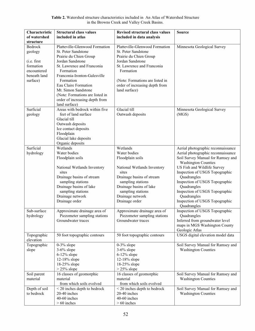
52

Table 2. Watershed structure characteristics included in An Atlas of Watershed Structure in the Browns Creek and Valley Creek Basins.

Characteristicof watershedstructure

Structural class valuesincluded in atlas

Revised structural class valuesincluded in data analysis

Source

Bedrockgeology

(i.e. firstformationencounteredbeneath landsurface)

Platteville-Glenwood FormationSt. Peter SandstonePrairie du Chien GroupJordan SandstoneSt. Lawrence and Franconia FormationFranconia-Ironton-Galesville FormationEau Claire FormationMt. Simon Sandstone(Note: Formations are listed inorder of increasing depth fromland surface)

Platteville-Glenwood FormationSt. Peter SandstonePrairie du Chien GroupJordan SandstoneSt. Lawrence and Franconia Formation

(Note: Formations are listed inorder of increasing depth fromland surface)

Minnesota Geological Survey

Surficialgeology

Areas with bedrock within five feet of land surfaceGlacial tillOutwash depositsIce contact depositsFloodplainGlacial lake depositsOrganic deposits

Glacial tillOutwash deposits

Minnesota Geological Survey(MGS)

Surficialhydrology

WetlandsWater bodiesFloodplain soils

National Wetlands Inventory sitesDrainage basins of stream sampling stationsDrainage basins of lake sampling stationsDrainage networkDrainage order

WetlandsWater bodiesFloodplain soils

National Wetlands Inventory sitesDrainage basins of stream sampling stationsDrainage basins of lake sampling stationsDrainage networkDrainage order

Aerial photographic reconnaissanceAerial photographic reconnaissanceSoil Survey Manual for Ramsey and Washington CountiesUS Fish and Wildlife SurveyInspection of USGS Topographic QuadranglesInspection of USGS Topographic QuadranglesInspection of USGS Topographic QuadranglesInspection of USGS Topographic Quadrangles

Sub-surfacehydrology

Approximate drainage area of Piezometer sampling stationsGroundwater traces

Approximate drainage area of Piezometer sampling stationsGroundwater traces

Inspection of USGS Topographic QuadranglesInferred from groundwater levelmaps in MGS Washington CountyGeologic Atlas

Topographicelevation

50 foot topographic contours 50 foot topographic contours USGS digital elevation model data

Topographicslope

0-3% slope3-6% slope6-12% slope12-18% slope18-25% slope> 25% slope

0-3% slope3-6% slope6-12% slope12-18% slope18-25% slope> 25% slope

Soil Survey Manual for Ramsey and Washington Counties

Soil parentmaterial

16 classes of geomorphicmaterial from which soils evolved

16 classes of geomorphicmaterial from which soils evolved


Depth of soilto bedrock

< 20 inches depth to bedrock20-40 inches40-60 inches> 60 inches

< 20 inches depth to bedrock20-40 inches40-60 inches> 60 inches


53

Table 2. (continued)

Characteristicof watershedstructure

Structural class valuesincluded in atlas

Revised structural class valuesincluded in data analysis

Source

Depth to zoneof saturation insoils

<12 inches12-24 inches<24 inches12-36 inches18-36 inches24-36inches24-42inches24-48 inches36-60 inches48-72 inches> 72 inches

<12 inches12-36 inches36-72 inches> 72 inches


Soilinfiltrationcapacity(Based on soilhydrologicgroup rating)

HighHigh to moderateModerate to lowLow

HighHigh to moderateModerate to lowLow


Soilpermeability

< 0.2 inches per hour0.2-6.0 inches per hour0.6-2.0 inches per hour2.0-20.0 inches per hour2.0-6.0 inches per hour6.0-20.0 inches per hour>20.0 inches per hour

< 6.0 inches per hour6.0-20.0 inches per hour>20.0 inches per hour


Frequency ofsoil flooding

NoneRareCommonFrequent

NoneRareCommonFrequent


Hydric soils Presence/absence of hydric soils(i.e. soils formed in a wetlandhydrologic regime)

Presence/absence of hydric soils Soil Survey Manual for Ramsey and Washington Counties

Soil erodibility Highly erosive soilPossibly erosive soilNot highly erosive soil

Highly erosive soilPossibly erosive soilNot highly erosive soil


Land cover Water bodyWetlandCrop landImperviousLawn (e.g. turfgrass aroundresidences)ForestShrub and grassland complex

Water bodyWetlandCrop landImperviousLawn (e.g. turfgrass aroundresidences)ForestShrub and grassland complex

Aerial photo and field reconnaissance

Land parcels Parcel boundaries Parcel boundaries Washington County Surveyor s Office

54

Table 3. Variables used to measure watershed structural characteristicsfor the stream and lake sample stations.

Watershed StructureCharacteristic

Variables Used to Measure Structural Characteristic

Bedrock geology* % basin occupied by St. Peter Sandstone deposits*% basin occupied by Prairie du Chien Group deposits*% basin occupied by Jordan Sandstone deposits*% basin occupied by Prairie du Chien Group or Jordan Sandstone deposits*% basin occupied by St. Lawrence-Franconia Formation deposits*

Surficial geology* % basin occupied by outwash deposits*% basin occupied by till deposits*

Slope % basin occupied by slopes less than 3%% basin occupied by slopes 3-6%% basin occupied by slopes > 6%% basin occupied by slopes 6-12%% basin occupied by slopes 12-18%% basin occupied by slopes 18-25%% basin occupied by slopes > 25%

Depth to bedrock % basin occupied by soils with depth to bedrock < 60 inches% basin occupied by soils with depth to bedrock > 60 inches

Depth to soil saturation % basin occupied by soils with depth to saturation < 72 inches% basin occupied by soils with depth to saturation > 72 inches

Soil infiltration capacity*

% basin occupied by soils with high infiltration capacity*% basin occupied by soils with moderately high infiltration capacity*% basin occupied by soils with high or moderately high infiltration capacity*% basin occupied by soils with moderately low infiltration capacity*% basin occupied by soils with low infiltration capacity*% basin occupied by soils with moderately low or low infiltration capacity*

Soil permeability* % basin occupied by soils with permeability < 6 inches per hour*% basin occupied by soils with permeability > 6 inches per hour*

Soil flooding % basin occupied by soils that are commonly or frequently flooded% basin occupied by soils that are never flooded

Hydric soils % basin occupied by hydric soils% basin occupied by non-hydric soils

Soil erodibility % basin occupied by highly erosive soils% basin occupied by potentially highly erosive soils% basin occupied by highly erosive or potentially highly erosive soils% basin occupied by not highly erosive soils

Land cover* % basin occupied by National Wetland Inventory Site*% basin occupied by surface water*% basin occupied by wetlands as interpreted from aerial photography*% basin occupied by surface water or by wetland as interpreted from aerial photography*% basin occupied by lawn*% basin occupied by impervious surfaces*% basin occupied by crop land*% basin occupied by lawn, impervious surfaces or crop land*% basin occupied by forest*% basin occupied by grassland complex*

NOTES: Variables identified with and asterisk (*) were also used to measure structural dimensions for thepiezometer and bedrock well stations.

55

Table 4. Key variables used to represent characteristics of watershed structurefor stream sample basins



Bedrock geology % basin occupied by Prairie du Chien Group or Jordan Sandstone depositsSurficial geology % basin occupied by till depositsSlope % basin occupied by slopes less than 3%

Log (base 10) of % basin occupied by slopes > 6%Depth to bedrock Log (base 10) % basin occupied by soils with depth to bedrock > 60 inchesDepth to soil saturation % basin occupied by soils with depth to saturation > 72 inchesSoil infiltration capacity

% basin occupied by soils with high infiltration capacity% basin occupied by soils with moderately low or low infiltration capacity

Soil permeability % basin occupied by soils with permeability < 6 inches per hourSoil flooding % basin occupied by soils that are never floodedHydric soils % basin occupied by non-hydric soilsSoil erodibility Log (base 10) % basin occupied by highly erosive soilsLand cover Log (base 10) % basin occupied by wetlands as interpreted from aerial

photographyLog (base 10) % basin occupied by impervious surfacesLog (base 10) % basin occupied by forest

Table 5. Key variables used to represent characteristics of watershed structurefor lake sample basins



Bedrock geology % basin occupied by Prairie du Chien Group or Jordan Sandstone depositsSurficial geology % basin occupied by till depositsSlope % basin occupied by slopes less than 3%

% basin occupied by slopes > 6%Depth to bedrock % basin occupied by soils with depth to bedrock > 60 inchesDepth to soil saturation % basin occupied by soils with depth to saturation > 72 inchesSoil infiltration capacity

% basin occupied by soils with high infiltration capacity% basin occupied by soils with moderately low or low infiltration capacity

Soil permeability % basin occupied by soils with permeability < 6 inches per hourSoil flooding % basin occupied by soils that are never floodedHydric soils % basin occupied by non-hydric soilsSoil erodibility Log (base 10) % basin occupied by highly erosive soilsLand cover % basin occupied by wetlands as interpreted from aerial photography

Log (base 10) % basin occupied by impervious surfaces% basin occupied by forest

56

Table 6. Key variables used to represent characteristics of watershed structurefor piezometer sample basins



Bedrock geology % basin occupied by Prairie du Chien Group or Jordan Sandstone depositsSurficial geology Log (base 10) % basin occupied by outwash depositsSoil infiltration capacity

Log (base 10) % basin occupied by soils with high infiltration capacityLog (base 10) % basin occupied by soils with moderately low or low infiltration capacity

Soil permeability % basin occupied by soils with permeability < 6 inches per hourLand cover Log (base 10) % basin occupied by surface water

Log (base 10) % basin occupied by wetlands as interpreted from aerial photographyLog (base 10) % basin occupied by surface water or by wetland as interpreted from aerial photography% basin occupied by lawnLog (base 10) % basin occupied by impervious surfaces% basin occupied by crop land% basin occupied by lawn, impervious surfaces or crop landLog (base 10) % basin occupied by forest

Table 7. Key variables used to represent characteristics of watershed structurefor bedrock well trace sample basins



Bedrock geology % basin occupied by Prairie du Chien Group or Jordan Sandstone depositsSurficial geology % basin occupied by outwash depositsSoil infiltration capacity

Log (base 10) % basin occupied by soils with high infiltration capacity% basin occupied by soils with moderately low or low infiltration capacity

Soil permeability % basin occupied by soils with permeability < 6 inches per hourLand cover Log (base 10) % basin occupied by surface water

Log (base 10) % basin occupied by wetlands as interpreted from aerial photography% basin occupied by surface water or by wetland as interpreted from aerial photography% basin occupied by lawnLog (base 10) % basin occupied by impervious surfaces% basin occupied by crop land% basin occupied by lawn, impervious surfaces or crop landLog (base 10) % basin occupied by forest

57

Table 8. Rotated factor structure of water quality variables for stream samplesin Valley Creek and Browns Creek.

FactorWater Quality Variable 1 2 3 4 5 6 7 8 9Temperature .05 .31 .04 -.54 .13 -.12 .15 -.34 .14Specific Conductivity .03 .66 -.09 .25 .08 -.104 .04 -.29 -.16pH* -.05 -.02 -.01 -.04 .03 -.04 .03 -.04 .89*Dissolved oxygen -.007 .01 -.002 .04 -.007 .03 -.04 .72 -.34% dissolved oxygen -.01 -.006 .02 .12 .14 -.08 -.02 .79* .24Total suspended solids* -.14 -.26 -.06 .07 -.02 .90* -.08 -.01 -.02Volatile suspended solids -.16 -.22 -.04 .04 -.05 .88 -.11 -.02 -.01% volatile suspended solids .16 .19 .27 .35 .06 -.36 .02 .04 .30Total phosphorous -.25 -.77 -.21 .12 .03 .35 .0009 -.04 -.08Dissolved phosphorous -.22 -.83 -.22 .16 .08 .03 .01 .0009 -.08Total nitrogen* .02 .14 -.10 .86* .14 .12 -.04 .02 -.03Dissolved nitrogen .08 .23 -.02 .83 .13 -.06 -.04 .04 .02Dissolved organic carbon -.08 -.53 .30 -.25 -.30 .15 -.04 -.28 -.08Dissolved inorganic carbon* .31 .86* -.10 .22 .06 -.15 .06 .04 -.03Alkalinity .30 .86 -.10 .21 .06 -.15 .06 .04 -.03Silicon .87 .16 -.28 -.01 -.15 -.10 .11 -.009 -.03Calcium* .92* .18 -.12 .11 .23 -.09 .002 -.002 -.01Magnesium .91 .18 -.10 .10 .29 -.10 -.03 -.00001 -.01Sodium -.18 -.03 .91 -.06 -.13 -.11 .21 -.02 -.02Potassium -.80 -.18 -.30 .06 -.05 .12 -.32 .005 -.02Iron* -.25 -.03 -.10 -.13 -.79* .09 -.15 -.07 -.01Sulfate .74 .17 -.16 .18 .45 .04 -.28 .02 -.01Chloride* .006 .01 .94* -.05 -.09 -.11 .14 -.02 -.03Aluminum -.77 -.12 -.35 .005 .10 .14 -.22 -.007 .003Barium -.29 .01 .44 -.02 .14 .16 .22 .10 .14Manganese .02 -.02 .36 -.06 -.74 -.08 -.21 -.07 -.06Strontium .94 .18 -.04 .02 .05 -.13 .18 -.008 -.01Fluoride .84 .18 -.21 .02 .05 .005 .22 .02 .03Bromide .58 .11 .07 0.06 .61 -.12 -.23 -.01 -.03Heavy oxygen* 0.30 .06 .36 -.11 .12 -.14 .82* -.06 .03Deuterium .38 .08 .27 -.09 .15 -.14 .82 -.06 .04% total variance explained 30.3% 13.4% 9.9% 7.0% 5.4% 4.6% 3.7% 3.3% 3.3%

NOTES: 1. Extraction Method: Principal Component Analysis. Rotation Method: Varimax with Kaiser Normalization. 2. Bold face* indicates variable selected as surrogate for each factor.

58

Table 9. Rotated factor structure of water quality variables for lake samplesin Valley Creek and Browns Creek.

FactorWater Quality Variable 1 2 3 4 5 6 7Temperature -.10 .001 -.07 .69 -.45 .004 -.42Specific Conductivity .82 .01 -.08 -.08 .18 .29 .04pH* -.34 -.02 .04 .73 -.32 .14 -.37Dissolved oxygen -.14 -.03 -.37 .70 .27 -.16 .24% dissolved oxygen* -.17 -.02 -.27 .90 .005 -.08 .01Total suspended solids* .005 .02 .90 -.10 .14 -.06 -.06Volatile suspended solids -.08 .02 .84 -.25 .19 -.005 -.05% volatile suspended solids -.12 -.02 -.28 -.64 -.01 .02 -.14Total phosphorous -.23 .05 .77 .24 .17 .004 .37Dissolved phosphorous -.39 .04 .55 .09 -.002 -.13 .47Total nitrogen* .08 .03 .30 .02 .89 .09 -.06Dissolved nitrogen .19 .02 .13 -.11 .89 -.11 -.13Dissolved organic carbon -.64 -.14 .30 -.12 .29 .26 .08Dissolved inorganic carbon .94 .05 -.09 -.06 .01 -.03 .04Alkalinity .94 .05 -.09 -.06 .01 -.03 .04Silicon .63 .73 -.03 -.02 -.06 -.02 .02Calcium* .95* -.19 -.03 -.09 .06 .01 -.04Magnesium .95 -.17 -.08 -.02 .04 -.01 -.07Sodium -.07 -.05 -.04 -.07 -.04 .96 .05Potassium -.27 .90 .15 .003 .11 .01 .17Iron* -.20 .91 .14 .06 -.04 -.05 .15Sulfate .89 .11 -.13 -.02 0.10 .06 .05Chloride* .16 .12 -.06 -.01 .01 .95 .12Aluminum -.02 .99 -.04 .002 -.02 .02 -.0005Barium -.02 .99 -.04 .002 -.01 .02 .001Manganese .04 .96 .05 -.06 .04 .02 -.05Strontium .77 .53 -.07 -.10 .04 .14 .05Fluoride .04 .99 -.05 -.005 .01 .04 .08Bromide -.01 .99 -.04 -.0001 -.02 .02 -.002Heavy oxygen -.90 .24 -.16 .12 -.09 .02 .12Deuterium -.84 .41 -.19 .08 -.07 .03 .12% total variance explained 26.7% 24.1% 9.7% 9.2% 7.1% 6.9% 4.6%


59

Table 10. Rotated factor structure of water quality variables for groundwater samplesin Valley Creek and Browns Creek.

FactorWater Quality Variable 1 2 3 4 5 6 7 8 9 10Temperature -.02 -.10 -.91 .15 -.06 -.10 .14 .08 .02 .04Specific Conductivity .26 -.12 .19 .31 -.07 -.23 .20 -.74 .01 .12pH* -.09 -.24 .18 -.17 .06 .20 -.08 .56* .04 .53Dissolved oxygen .10 -.14 .25 .92 .06 .02 -.15 -.09 .05 .01% dissolved oxygen* .12 -.15 .10 .94* .04 .002 -.16 .01 .06 .01Total suspended solids* .09 .002 .93* .21 .09 .27 .02 -.22 -.03 -.03Volatile suspended solids .06 .01 .90 .33 .08 -.02 .04 .06 .0007 .04% volatile suspended solids .13 .02 -.23 .23 -.03 -.14 .04 .80 .10 .20Total phosphorous .38 .10 -.08 .08 .0006 .04 .04 .10 -.07 .83Dissolved phosphorous .30 .31 .06 -.44 -.18 .12 .02 .33 .08 -.02Total nitrogen* .16 -.17 .06 -.05 -.03 -.22 -.09 .26 .72* -.26Dissolved nitrogen -.13 -.13 -.05 .08 .03 .13 .02 -.09 .80 .12Dissolved organic carbon -.02 -.004 .001 -.12 .47 .71 -.008 .27 -.07 -.20Dissolved inorganic carbon* .90* -.05 .14 .06 .01 -.007 .19 .08 .08 .06Alkalinity .90 -.05 .14 .06 .01 -.007 .19 .08 .08 .06Silicon -.33 .70 -.11 -.08 .04 -.48 -.09 -.05 .14 .16Calcium* .02 -.25 -.13 .09 .07 -.57 .18 .09 .62* -.04Magnesium .72 -.47 -.21 .02 .20 -.15 -.09 -.22 .15 .03Sodium .14 -.16 .15 .08 .83 .25 .08 .13 -.13 .02Potassium .75 -.29 -.13 .11 .19 -.03 -.02 -.08 -.36 .15Iron* .17 .74* -.006 -.24 -.12 .28 .34 -.10 .02 .16Sulfate .10 -.62 -.11 .11 .35 -.30 -.24 -.04 .19 .09Chloride* .02 .06 .13 .04 .91* -.05 .25 -.03 .17 -.04Aluminum -.10 .30 .05 .07 .02 .83 -.004 -.01 .03 .26Barium .41 .10 -.08 -.19 -.04 .05 .78 -.08 -.14 -.01Manganese .62 .27 -.06 -.16 .11 .15 .47 -.23 -.27 18Strontium -.30 0.4 -09 -.008 .17 -.42 .61 .34 .10 -.04Fluoride -.56 -.12 .02 -.17 -.61 .07 .28 .31 .007 -.09Bromide .15 .004 .004 -.13 .16 -.01 .78 -.10 .10 .02Heavy oxygen* -.10 .92* .05 -.06 .09 .08 -.05 .03 -.21 -.01Deuterium -.09 .93 .04 -.12 .06 .08 -.03 .02 -.17 -.05% total variance explained 13.8% 13.0% 9.5% 8.2% 8.0% 7.9% 7.8% 7.2% 6.6% 4.4%


60

Table 11. Mean values of 31 water quality variables measured in Valley Creekand Browns Creek stream samples under different flow regimes.

Flow RegimeWater Quality Variable Low Medium High OverallTemperature (°Celsius) 8.89a 11.94b 9.35a 10.94Specific Conductivity (_ S) 454.98a 457.48a 386.57b 437.43pH 7.67a 7.45b 7.42b 7.46Dissolved oxygen (mg/l) 12.21a 11.69a 11.65a 11.73% dissolved oxygen 107.15a 102.46b 102.42b 102.89Total suspended solids (mg/l) 9.10a 13.38a 108.98b 39.69Volatile suspended solids 3.66a 5.15a 22.15b 9.76% volatile suspended solids 70.24a 59.60b 41.40c 55.51Total phosphorous (_ g/l) 64.28a 68.56a 350.31b 146.89Dissolved phosphorous (_ g/l) 32.74a 42.43a 207.47b 87.64Total nitrogen (mg/l) 4.74a 4.15b 4.27ab 4.24Dissolved nitrogen (mg/l) 4.38a 4.08a 3.98a 4.08Dissolved organic carbon(mg/l)

1.80a 2.57b 4.03c 2.91

Dissolved inorganic carbon(mg/l)

42.14a 41.71a 30.46b 38.60

Alkalinity (meq/l) 3.53a 3.50a 2.59b 3.25Silicon (mg/l) 5.89a 5.99a 5.44b 5.83Calcium (mg/l) 39.21a 39.27a 35.50b 38.21Magnesium (mg/l) 16.25a 16.29a 14.67b 15.83Sodium (mg/l) 8.48a 8.68b 8.38c 8.57Potassium (mg/l) 3.25a 3.11a 3.87b 3.33Iron (mg/l) 0.11a 0.11a 0.12a 0.11Sulfate (mg/l as S) 3.29a,b 3.25b 3.07a 3.20Chloride (mg/l) 17.36a 17.70a 16.99a 17.47Aluminum (mg/l) 0.04a 0.04a 0.05b 0.04Barium (mg/l) 0.04a 0.04a 0.04a 0.04Manganese (mg/l) 0.04a 0.04a 0.04a 0.04Strontium (mg/l) 0.05a 0.05a 0.05b 0.05Fluoride (mg/l) 0.11a 0.11a 0.10b 0.11Bromide (mg/l) 0.007a,b 0.007a 0.006b -.007Heavy oxygen _18 O -9.86a -9.72a -10.18b -9.86Deuterium _D -70.22a -69.20a -72.50b -70.22

NOTES: 1. Values followed by identical letters (a,b,c) are not significantly different at p<.05 using the ScheffeMultiple Comparison test. 2. Values in bold face represent water quality variables examined in the stream sample analysis.

61

Table 12. Coefficients of partial correlation between water quality variables and watershed structure variablescontrolling for effects of flow regime in stream water samples.

Water Quality Variables (dependent variables)Watershed Structure Variable(independent variables) pH %

dissolvedoxygen

Log 10 totalsuspended

solids

Log 10 totalphosphorous

Totalnitrogen

Dissolvedinorganic

carbon

Calciumion

Log 10ironion

Log 10chloride

ion

Heavyoxygen

Log % watershed area in wetland cover -.15** -.82** -.10* .39** .54** .25*Log % watershed area in impervious cover -.26** .18** .17** -.73** -.38** -.50** .77** .38**Log % watershed area in forest cover .13* .15** -.16** -.44** -.10* .45** .42** -.62**Log % watershed area containing highly erosivesoils

-.14* .22** .40** .51** -.50** -.28*

% watershed area containing soils in HydrologicGroup A

-.25** -.47** .26** .36**

% watershed area area containing soils inHydrologic Groups C/D

.17** .48**

% watershed area containing soils that never flood .23** -.19** -.20** .80** .26** .25** -.48** -.35**% watershed area containing soils with saturationzone deeper than 72 inches

.24** -.20** -.27** .76** .35** .34** -.52** -.44** -.24*

% watershed area containing soils withpermeability < 6 in./hr.

.78** .12* -.63** -.40**

Log % watershed area containing soils withbedrock deeper than 60 inches

-.31** .20** .21** -.88** -.31** -.26* .48** .47** .27*

% watershed area containing soils that are nothydric

.23** -.21** -.22** .81** .29** .26* -.49** -.34**

% watershed area containing till surface geologicformation

.13* .19** .25** -.35** -.53** .43**

% watershed area containing soils with slopes <3%

-.26** .17** .18** -.69** -.15** .54**

Log of % watershed area containing soils withslopes > 6%

.14* -.21** -.53** -.32** .58** .34**

% watershed area containing Jordan or Prairie duChien bedrock geologic formation

-.27** .12** -.58** .28*

NOTES: Only significant (p < 0.05) partial correlation coefficients are shown. ** p < 0.01

* p < 0.05

62

Table 13. Coefficients of correlation between water quality variablesand watershed structure variables in lake samples.

Water Quality Variables (dependent variables)Watershed Structure Variable (independent variables) Log 10

pHa%

dissolvedoxygena


solids

Log 10total

nitrogen

Calciumion

Log 10iron ion

Chlorideion


% Watershed in wetland cover .34*Log % watershed in impervious cover .31* .33* .54**% watershed in forest cover .42**Log % watershed containing highly erosive soils .33* .53**% watershed containing soils in Hydrologic Group A% watershed containing soils in Hydrologic GroupsC/D

-.36* -.39*

% watershed containing soils that never flood .43** .32*% watershed containing soils with saturation zonedeeper than 72 inches

.59** .45**

% watershed containing soils with permeability < 6in./hr.

.32*

% watershed containing soils with bedrock deeperthan 60 inches

.35*

% watershed containing soils that are not hydric .37* .45** .35* .38*% watershed containing till surface geologicformation

-.63** -.48

% watershed containing soils with slopes < 3% -.34*% watershed containing soils with slopes > 6%% watershed containing Jordan or Prairie du Chienbedrock geologic formation

.59**

NOTES: Only significant (p<0.05) correlation coefficients are shown.** p < 0.01 * p < 0.05 a None of the watershed structure variables exhibited significant relationships with this water quality variable.

63

Table 14. Coefficients of correlation between water quality variablesand watershed structure variables in piezometer samples.

Water Quality Variables (dependent variables)Watershed Structure Variable(independent variables) Log 10

Dissolvedphosphorous

Log 10dissolvednitrogen

Dissolvedinorganic

carbon

Calciumion

Ironion

Chlorideion

Log10heavyoxygen

Log 10 % watershed in lakes -.74** .57* .80**Log 10 % watershed in wetlandcover

-.70* -.60** -.67** .69** .83**

% watershed in water or wetland -.70** -.53* .70** .87**Log 10 % watershed in imperviouscover

-.72* -.61**

% watershed in lawn cover -.88** -.62* -.70**% watershed in lawn, impervious orcrops (i.e. total disturbed area)

.54* -.78** -.91**

% watershed in crop cover .65** -.78** -.89**Log 10 % watershed in forest cover -.76* .58*Log 10 % watershed containing soilsin Hydrologic Group A

-.66* .71**

Log 10 % watershed containing soilsin Hydrologic Groups C/D

.80** .57*

% watershed containing soilswith permeability < 6 in./hr.Log 10 % watershed containingoutwash surface geologic formation

-.75* .78** .85**

% watershed containing Jordan orPrairie du Chien bedrock geologicformation

.53* .70**

NOTES: Only significant (p < 0.05) correlation coefficients are shown.** denotes p < 0.01* denotes p < 0.05

64

Table 15. Coefficients of correlation between water quality variablesand trace area structure variables in bedrock well samples.

Water Quality Variables (dependent variables)Trace Area Structure Variable(independent variables) Log10

Dissolvedphosphorous a

Dissolvednitrogen

Dissolvedinorganic

carbon

Calciumion

Ironion

Chlorideion a

Log10heavyoxygen

Log % trace area in lakes -.52* -.61**Log % trace area in wetland cover% trace area in water or wetland -.65**Log % trace area in impervious cover .75**% trace area in lawn cover% trace area in lawn, impervious or crops(i.e. total disturbed area)

.64** .55*

% trace area in crop cover -.63*Log % trace area in forest cover -.60**Log % trace area containing soilsin Hydrologic Group A

-.79** -.69**

% trace area containing soilsin Hydrologic Groups C/D

-.62**

% trace area containing soilswith permeability < 6 in./hr.

.62**

% trace area containing outwashsurface geologic formation

.60*

% trace area containing Jordan orPrairie du Chien bedrock geologicformation

.56** .71**

NOTES: Only significant (p < 0.05) correlation coefficients are shown.** denotes p < 0.01* denotes p < 0.05a None of the trace area structure variables exhibited significant relationships with this water quality variable.

65

Table 16. Regression coefficients and coefficients of determination derived from regressionof water quality variables on watershed structure variables for stream water samples.

Water Quality Variables (dependent variables)Watershed Structure Variable(independent variables) pH % dissolved

oxygenLog 10 totalsuspended

solids


Totalnitrogen

Constant 5.91** 585.06** 11.66** 2.53** 25.44**Flow Regime (Flow) -0.08 -1.15 7.73** 4.70** -11.20**Log % Watershed in wetland cover (Wetland) 8.84** -1.68**Log % watershed in impervious cover(Impervious)

0.61**

Log % watershed in forest cover (Forest) -0.81**Log % watershed containing highly erosive soils(Erosive)

-5.12**

% watershed containing soils in HydrologicGroup A (HydroA)% watershed containing soils in HydrologicGroups C/D (HydroC/D)

0.03**

% watershed containing soils that never flood(NoFlood)% watershed containing soils with saturation zonedeeper than 72 inches (Water Table)

-.02**

% watershed containing soils with permeability <6 in./hr. (Perm)

-0.74** 0.03**

Log % watershed containing soils with bedrockdeeper than 60 inches (Deep Bedrock)

-1.16* -220.46** -11.52**

% watershed containing soils that are not hydric(No Hydric)

-0.03**

% watershed containing till surface geologicformation (Till)

0.007**

% watershed containing soils with slopes < 3%(Flat)Log of % watershed containing soils with slopes >6% (Steep)

2.27**

% watershed containing Jordan or Prairie duChien bedrock geologic formation (Jordan-PdC)Interaction of Flow x Wetland -0.67** 1.15**Interaction of Flow x ImperviousInteraction of Flow x Forest -0.75** 2.32**Interaction of Flow x ErosiveInteraction of Flow x HydroAInteraction of Flow x HydroC/D 0.05**Interaction of Flow x NoFloodInteraction of Flow x Water Table -0.11**Interaction of Flow x PermInteraction of Flow x Deep BedrockInteraction of Flow x No Hydric -.04** 0.18**Interaction of Flow x Till -.03**Interaction of Flow x FlatInteraction of Flow x Steep -4.46**Interaction of Flow x Jordan-PdC

Coefficient of determination (Adjusted R2) 0.05 0.22 0.50 0.64 0.86F-value of regression model 4.74** 19.93** 90.12** 137.31** 254.22**Degrees of freedom 4,293 4,271 6,529 6,451 10,411

NOTES: Only significant (p < 0.05) are shown.** p < 0.01 * p < 0.05

66

Table 16. Regression coefficients and coefficients of determination derived from regressionof water quality variables on watershed structure variables for stream water samples (continued).

Water Quality Variables (dependent variables)Watershed Structure Variable(independent variables) Dissolved

inorganiccarbon

Calciumion

Log 10iron ion

Log 10chloride

ion

Heavyoxygen

Constant -103.14** 47.86** .11 1.63** -15.01**Flow Regime (Flow) -125.29** -83.25** .99** -0.36* -10.06**Log % Watershed in wetland cover (Wetland)Log % watershed in impervious cover(Impervious)

26.02* 0.84** 9.01**

Log % watershed in forest cover (Forest) -1.88**Log % watershed containing highly erosive soils(Erosive)

-0.74**

% watershed containing soils in HydrologicGroup A (HydroA)% watershed containing soils in HydrologicGroups C/D (HydroC/D)

1.01**

% watershed containing soils that never flood(NoFlood)% watershed containing soils with saturationzone deeper than 72 inches (Water Table)

1.31**

% watershed containing soils with permeability< 6 in./hr. (Perm)Log % watershed containing soils with bedrockdeeper than 60 inches (Deep Bedrock)

-161.67**

% watershed containing soils that are not hydric(No Hydric)

0.004**

% watershed containing till surface geologicformation (Till)

-0.31** -0.69**

% watershed containing soils with slopes < 3%(Flat)

0.30** 0.04**

Log of % watershed containing soils with slopes> 6% (Steep)% watershed containing Jordan or Prairie duChien bedrock geologic formation (Jordan-PdC)Interaction of Flow x Wetland 17.03** 22.54** .12**Interaction of Flow x Impervious -8.13**Interaction of Flow x Forest 27.79** .23* 9.87**Interaction of Flow x ErosiveInteraction of Flow x HydroAInteraction of Flow x HydroC/DInteraction of Flow x NoFlood 0.89**Interaction of Flow x Water Table 0.80*Interaction of Flow x PermInteraction of Flow x Deep BedrockInteraction of Flow x No HydricInteraction of Flow x TillInteraction of Flow x Flat -0.03**Interaction of Flow x SteepInteraction of Flow x Jordan-PdC

Coefficient of determination (Adjusted R2) 0.72 0.73 0.66 0.83 0.64**F-value of regression model 126.91** 46.06** 35.24** 69.02** 29.99Degrees of freedom 9,424 5,80 4,65 6,78 4,62

NOTES: Only significant (p < 0.05) are shown.** p < 0.01; * p < 0.05

67

Table 17. Regression coefficients and coefficients of determination derived from regressionof water quality variables on watershed structure variables for lake water samples.


pHa%

dissolvedoxygena


solids

Log 10total

nitrogen

Calciumion

Log 10iron ion

Chlorideion


Constant 0.28 -.043 20.58** 5313.88** -6.07 0.24% Watershed in wetland coverLog % watershed in impervious cover 0.63* 29.20** 22.17**% watershed in forest cover -0.005* 161.41** -0.01**Log % watershed containing highly erosive soils% watershed containing soils in Hydrologic Group A -229.39**% watershed containing soils in Hydrologic Groups C/D% watershed containing soils that never flood% watershed containing soils with saturation zonedeeper than 72 inches

-0.02**

% watershed containing soils with permeability < 6in./hr.% watershed containing soils with bedrock deeper than60 inches% watershed containing soils that are not hydric 0.01** 0.04**% watershed containing till surface geologic formation -.048** -108.69**% watershed containing soils with slopes < 3%% watershed containing soils with slopes > 6% 0.01**% watershed containing Jordan or Prairie du Chienbedrock geologic formation

0.18**

Coefficient of determination (Adjusted R2) 0.07 0.19 0.50 0.45 0.56 0.47F-value of regression model 4.48* 5.40* 17.7** 13.56** 22.65** 9.14**Degrees of freedom 1,43 2,35 2,32 3,43 2,32 4,33

NOTES: Only significant (p < 0.05) coefficients are shown.** p < 0.01 * p < 0.05 a Regression analysis failed to generate a significant (p < 0.05) model.

68

Table 18. Regression coefficients and coefficients of determination derived from regressionof water quality variables on watershed structure variables for piezometer samples.


Dissolvedphosphorous

Log 10Dissolvednitrogen

Dissolvedinorganic

carbon

Calciumion

Ironion

Chlorideion

Log10heavyoxygen

Constant 1.30 1.37** 48.88** 89.91** -5.76** -60.31** .05Log 10 % watershed in lakes -7.36**Log 10 % watershed in wetland cover 1.76** -22.35**% watershed in water or wetland .23** .02**Log 10 % watershed in impervious cover% watershed in lawn cover -.13**% watershed in lawn, impervious or crops(i.e. total disturbed area)% watershed in crop cover -1.89**Log 10 % watershed in forest cover 5.68*Log 10 % watershed containing soilsin Hydrologic Group ALog 10 % watershed containing soilsin Hydrologic Groups C/D

5.43*

% watershed containing soilswith permeability < 6 in./hr.Log 10 % watershed containing outwashsurface geologic formation

44.21**

% watershed containing Jordan orPrairie du Chien bedrock geologicformation

-.12*

Coefficient of determination (Adjusted R2 ) .88 .74 .53 .77 .83 .71 .83F-value of regression model 22.84** 26.04** 20.01** 24.42** 34.63** 35.14** 69.08**Degrees of freedom (3,6) (1,8) (1,16) (2,12) (2,12) (1,13) (1,13)

NOTES: Only significant (p < 0.05) coefficients are shown.** denotes p < 0.01* denotes p < 0.05

69

Table 19. Regression coefficients and coefficients of determination derived from regressionof water quality variables on trace area structure variables for bedrock well samples.

Water Quality Variables (dependent variables)Trace Area Structure Variable(independent variables) Log10

DissolvedPhosphorousa

Dissolvednitrogen

Dissolvedinorganic

carbon

Calciumion

Ironion

Chlorideiona

Log10heavyoxygen

Constant -1.73 53.50** 44.92** -.51 .44**Log % trace area in lakesLog % trace area in wetland cover% trace area in water or wetlandLog % trace area in impervious cover 5.29**% trace area in lawn cover -.009*% trace area in lawn, impervious or crops(i.e. total impervious area)

.30*

% trace area in crop coverLog % trace area in forest coverLog % trace area containing soilsin Hydrologic Group A

-12.43**

% trace area containing soilsin Hydrologic Groups C/D% trace area containing soilswith permeability < 6 in./hr.% trace area containing outwashsurface geologic formation% trace area containing Jordan orPrairie du Chien bedrock geologicformation

.04**

Coefficient of determination (Adjusted R2 ) .54 .60 .26 .47 .33F-value of regression model 19.55** 29.91** 6.52* 15.31** 6.46*Degrees of freedom (1,15) (1,18) (1,15) (1,15) (1,10)

NOTES: Only significant (p < 0.05) coefficients are shown.** p < 0.01 * p < 0.05 a Regression analysis failed to generate a significant (p < 0.05) model.

d.g. pitt, j.e. almendinger, r. bell, and s. roos final .... pitt, j.e. almendinger, r. bell, and s....

Documents