dft md part1
DESCRIPTION
Density functional theory and molecular dynamicsTRANSCRIPT

Dr. Markus Drees, TU München
Introduction to Computational Chemistry for
Experimental Chemists... (Part 1/2)
Universität
Augsburg
Universität
Regensburg
11th PhD seminar, Garching, September 12th 2008

Outline of today
A) What is computational chemistry?Definitions - Methods - Types of calculations
B) From a Formula to calculated Properties
Graphical interfaces - input files - basis sets - calculation - output analysis
C) How to evaluate Mechanisms with Computational Chemistry
Mechanism theorems - energetic evaluation - transition states and kinetics
D) A Word on Costs and Accuracy
Phrases of prejudice - computational costs - accuracy

A) What is computational chemistry?Definitions - Methods - Types of calculations

A) What is Computational Chemistry? - Definitions
Chemistry, that is investigated in silico
Computational Chem. Cheminformatics
- Storage and analysis of compound
data (databases!)
- Virtual screening (identification of
targets in pharmacy)
- QSAR => quantitative structure-
activity relationship
==> related field: statistics
- Simulation / Modelling of structural
features
- Calculation of molecular properties
and energies
- Ab initio (simulation from the
beginning) and molecular mechanics
-Quantum / Molecular dynamics
==> related field:
theoretical chemistry
A) What is Computational Chemistry? - Method classes (I)
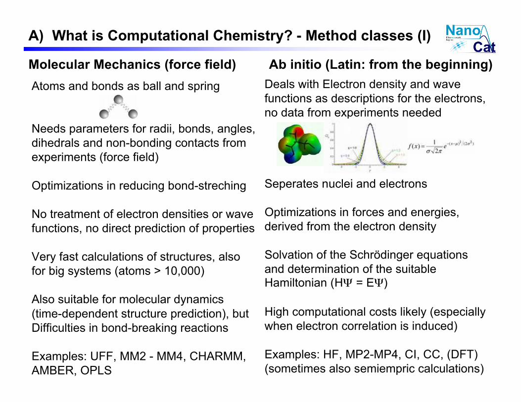
Molecular Mechanics (force field) Ab initio (Latin: from the beginning)
Atoms and bonds as ball and spring
Needs parameters for radii, bonds, angles,
dihedrals and non-bonding contacts from
experiments (force field)
Optimizations in reducing bond-streching
No treatment of electron densities or wave
functions, no direct prediction of properties
Very fast calculations of structures, also
for big systems (atoms > 10,000)
Also suitable for molecular dynamics
(time-dependent structure prediction), but
Difficulties in bond-breaking reactions
Examples: UFF, MM2 - MM4, CHARMM,
AMBER, OPLS
Deals with Electron density and wave
functions as descriptions for the electrons,
no data from experiments needed
Seperates nuclei and electrons
Optimizations in forces and energies,
derived from the electron density
Solvation of the Schrödinger equations
and determination of the suitableHamiltonian (H! = E!)
High computational costs likely (especially
when electron correlation is induced)
Examples: HF, MP2-MP4, CI, CC, (DFT)
(sometimes also semiempric calculations)

A) What is Computational Chemistry? - Method classes (II)
Semiempirics Density functional theory
Mixture of force-field and ab initio
calculation
Reduction of the system (Hueckel => onlyvalid for "-electrons)
Treatment only of valence eletrons
(AM1, MNDO, PM3-PM5)
Simple Hamiltonian used to solve a
simplier Schroedinger equations in
combination with force-field parameters
==> not always suitable for all
configurations of an element
Fast calculations in comparison the ab
initio methods
Also suitable for molecular dynamics
(time-dependent structure prediction),
even for reaction prediction
Correlation between wave function and
electron density (Hohenberg-Kohn)
=> All physical properties derived from
wave functions are also predictable by
electron density
Problem: Exact functional to calculate
electron correlation and exchange is not
exactly known! => All DFT “methods“ are
approximations of this functional
Good treatment of electron correlation
(better than in HF, while with less cost
than in post-HF methods)
Problems with intermolecular interactions
(dispersion, van der Waals-forces)
Examples:B3LYP, PBE, BLYP, BP88,
O3LYP, MPW1K, ...

A) What is Computational Chemistry? - Method classes (III)
QM/MM (or Hybrid Calculation)
Useful for larger molecules (biochemistry!) or solvent systems:
Distribution of the molecule into at least two parts: a QM part and a MM part
QM: normally the reaction center (higher accuracy)
MM: expresses the sterically more demanding sites that play only the role of
spectators.
Example: ONIOM

A) What is Computational Chemistry? - Calculation types (I)
- Geometry optimization of a ground state
Minimizes the energy, while intramoleculare forces are brought to 0.
Needs a structural starting point from the user.
Delivers the best structure an its total electronic energy
- Frequency calculation
Delivers the force constants and the vibrational frequencies
Simulations IR and Raman Spectra
Distinguishes a ground state from a transition state (number of negative frequencies)
Delivers thermodynamical data (enthalpy, entropy, free energy, heat capacities, ...)
- Search for a transition state of a chemical reaction
Optimizies the initial structure, while intramoleculare forces are brought to 0.
Follows the most negative frequency of the initial structure
Some algorithms determine the initial TS structure from the geometry of the educt(s)
and product(s)
Determination of barrier heights and kinetics (in combination with frequency
calculation)
To be considered today!

A) What is Computational Chemistry? - Calculation types (II)
- Population analysis
Determines the distribution of the electrons into the molecular orbitals
Delivers dipole moments
Creates graphical expressions of orbitals
- NMR calculation
Simulates the external field of the NMR source as perturbation for the
electron density
Delivers chemical shifts (in combination with a standard) and - very time consuming -
even coupling constants
- UV/VIS calculation
Calculates the most feasible electron excitations
Methods: time-dependent DFT or CIS (configuration interaction - singlets)
- Solvation energies
Implicit methods (SCRF) via correlation of an external reaction field in relation to the
polarity of the solvent, solvent models: PCM, Dipole, ...
Explicit calculations (addition of the solvent molecules to molecular systems) are more
time consuming than implicit methods
To be considered in part 2!

B) From a Formula to calculated Properties Graphical interfaces - input files - basis sets - calculation -
output analysis

B) From a formula to calculated properties - programs
Examples for program suites:
-GAUSSIAN
-NWCHEM
-GAMESS
-TURBOMOLE
-ADF (DFT only)
-MOPAC (Semiempric and HF)
-TINKER (Molecular mechanics)

B) From a formula to calculated properties - graphical interfaces
Graphical interfaces as source for initial geometries:
(GaussView as example)
Also possible is the use of programs like Chem3D or the conversion of crystal
structure data into xyz coordinates or Z-matrix.

B) From a formula to calculated properties - input files
Input files contain: - the level of theory (method and basis sets)
- (initial) geometry of the investigated system
- system requirements (no. of proceesors, memory)
- additional data depending on the type of calculation
Example: Optimization of Ammonia%chk=nh3_zmat.chk
%mem=3800MB
%nproc=2
#opt b3lyp/6-311++G**
Ammonia as ZMat
0 1 N
H 1 B1
H 1 B2 2 A1
H 1 B3 3 A2 2 D1
B1 1.00000000
B2 1.00000000
B3 1.00000000
A1 109.47120255
A2 109.47125080 D1 -119.99998525
%chk=nh3_xyz.chk
%mem=3800MB
%nproc=2
#opt b3lyp/6-311++G**
Ammonia in cart coordinates
0 1 N 0.00000000 0.00000000 0.00000000
H 0.00000000 0.00000000 1.00000000
H 0.94280915 0.00000000 -0.33333304
H -0.47140478 -0.81649655 -0.33333304
Z matrix (left) vs.
cart. coordinates (right)
taken from Gaussian03

B) From a formula to calculated properties - basis sets (I)
Mathematical functions to describe the electrons (wave character)
Mostly used: Linear combinations of gauss functions
Linear combinations of Gauss functions are flexible enough to model
s, p, d and f orbitals!

B) From a formula to calculated properties - basis sets (II)
Minimal basis: STO-NG (N primitive Gauss functions as linear combination
for one orbital each) => Lousy accuracy
Often used: Split valence basis set
(Inner shell orbitals with other numbers of gauss functions than valence shell
orbitals)
3 - 21G
Sum of 3 Gauss functions for inner shell orbitals
Separation for valence shell orbitals into two basis functions consisting of 2
and 1 Gauss functions (carbon: 1s=3, 2s=3, 2p=3: 9 Gaussian functions)
6 - 31G
Sum of 6 Gauss functions for inner shell orbitals
Separation for valence shell orbitals into two basis functions consisting of 3
and 1 Gauss functions (carbon: 1s=6, 2s=4, 2p=4: 14 Gaussian functions)
6 - 311G
Sum of 6 Gauss functions for inner shell orbitals
Separation for valence shell orbitals into three basis functions consisting of 3
and a pair of independent gauss func. (C: 1s=6, 2s=5, 2p=5: 16 Gauss func.)
B) From a formula to calculated properties - basis sets (III)
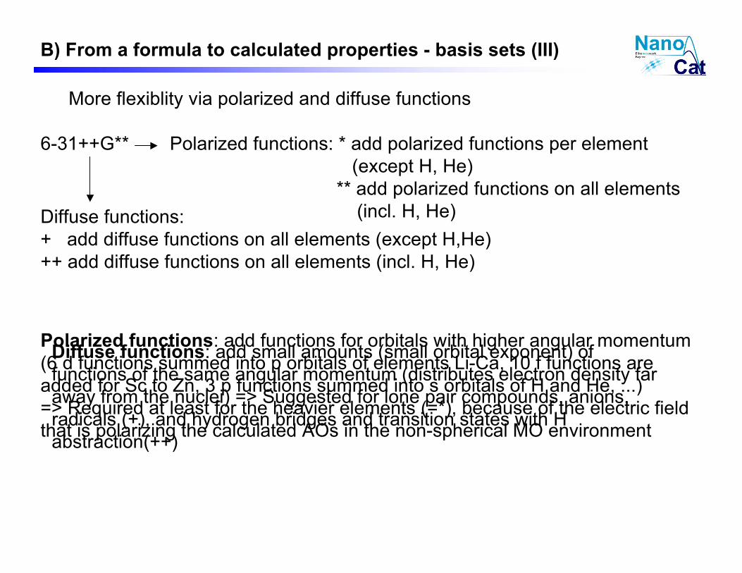
More flexiblity via polarized and diffuse functions
6-31++G** Polarized functions: * add polarized functions per element
(except H, He)
** add polarized functions on all elements
(incl. H, He)Diffuse functions:
+ add diffuse functions on all elements (except H,He)
++ add diffuse functions on all elements (incl. H, He)
Polarized functions: add functions for orbitals with higher angular momentum
(6 d functions summed into p orbitals of elements Li-Ca, 10 f functions are
added for Sc to Zn, 3 p functions summed into s orbitals of H and He, ...)
=> Required at least for the heavier elements (=*), because of the electric field
that is polarizing the calculated AOs in the non-spherical MO environment
Diffuse functions: add small amounts (small orbital exponent) of
functions of the same angular momentum (distributes electron density far
away from the nuclei) => Suggested for lone pair compounds, anions,
radicals (+), and hydrogen bridges and transition states with H
abstraction(++)

B) From a formula to calculated properties - basis sets (III)
More flexiblity via polarized and diffuse functions
6-31++G** Polarized functions: * add polarized functions per element
(except H, He)
** add polarized functions on all elements
(incl. H, He)Diffuse functions:
+ add diffuse functions on all elements (except H,He)
++ add diffuse functions on all elements (incl. H, He)
Diffuse functions: add small amounts (small orbital exponent) of
functions of the same angular momentum (distributes electron density far
away from the nuclei) => Suggested for lone pair compounds, anions,
radicals (+), and hydrogen bridges and transition states with H
abstraction(++)

B) From a formula to calculated properties - basis sets (IV)
What about heavier atoms (transition metals)?
Description of metals via ECPs (Effective core potential)
#Valence shell orbitals via basis functions
#Inner shell electrons summed up into an averaged field
#Relativistic effects easily incorporated
Examples: LANL2DZ / Hay-Wadt; Stuttgart-Dresden-(Köln)-ECPs
Suggestions for suitable basis sets (number of atoms < 90):
6-31G* is regarded to be the minimum requirement for publications
Smaller systems (number of atoms < 20): 6-311+G** might be useful
Anions, Radicals: 6-31+G* might be required

B) From a formula to calculated properties - calculations
From the basis set to a valid wave function: SCF cycle
Complex evaluation of Integrals!
SCF = self-consistent field

B) From a formula to calculated properties - calculations (II)
Geometry Optimization: also a calculation cycle
Initial
structure
SCF procedure
(Determination of the wave
function and the energy)
Calculation of
orbital energies
Check for reaching the thresholds in
forces and changes in coordinates
and SCF energy down to 0?
Algorithm for determing the
geometry for the next point on
energy surface
Final summary of optimized geometry
End of optimzation run
First derivative of the SCF energy
with respect to the vector of location
For TS searches: also evaluation of
the second derivatives (Hessian
matrix)
YES
NO

B) From a formula to calculated properties - calculations (III)
Geometry Optimization: Minimum versus Transition state
Reactant(s) (Local Minimum)
Transition state
(1st order saddle point)Product(s) (Local Minimum)
Potential Energy Surface (PES)

B) From a formula to calculated properties - calculations (IV)
Transition state searches - Strategies
The search for transition states is one of the toughest businesses in
computational chemistry.
=> Mostly no automaticity, human interaction is needed
Strategies:
A) Draw your TS structure guess as accurate as you think.
Most negative eigenvector is followed. This might be also an unwanted
motion in the molecule (e.g. methyl rotation).
B) Pre-optimization
Draw the molecule with a reasonable geometry especially at the reaction
center. Freeze the reaction coordinate(s) and make a normal geometry
optimization (to avoid other unwanted modes).
Open the frozen coordinates and search the TS.

B) From a formula to calculated properties - output analysis
Analysis of output files: text file or graphical tools (GaussView, MOLDEN)
Geometry optimization:
Intermediate step: SCF Done: E(RB+HF-LYP) = -760.849791059 A.U. after 14 cycles
Convg = 0.4573D-08 -V/T = 2.0696 S**2 = 0.0000
Item Value Threshold Converged?
Maximum Force 0.061492 0.000450 NO
RMS Force 0.005240 0.000300 NO
Maximum Displacement 0.188036 0.001800 NO
RMS Displacement 0.044821 0.001200 NO
Predicted change in Energy=-1.175625D-02

B) From a formula to calculated properties - output analysis (II)
Optimization accomplished: Item Value Threshold Converged?
Maximum Force 0.000011 0.000450 YES
RMS Force 0.000001 0.000300 YES
Maximum Displacement 0.001232 0.001800 YES RMS Displacement 0.000269 0.001200 YES
Predicted change in Energy=-1.834641D-09
Optimization completed.
-- Stationary point found.
----------------------------
! Optimized Parameters !
! (Angstroms and Degrees) !
-------------------------- --------------------------
! Name Definition Value Derivative Info. !
-------------------------------------------------------------------------------- ! R1 R(1,2) 1.7311 -DE/DX = 0.0 !
! R2 R(1,3) 1.7724 -DE/DX = 0.0 !
! R3 R(1,4) 2.3156 -DE/DX = 0.0 !
! R4 R(1,20) 2.4801 -DE/DX = 0.0 !
! R5 R(1,21) 2.5229 -DE/DX = 0.0 !
! R6 R(1,22) 2.5034 -DE/DX = 0.0 !
! R7 R(1,23) 3.156 -DE/DX = 0.0 !
! R8 R(1,24) 2.4604 -DE/DX = 0.0 !
! R9 R(1,25) 3.163 -DE/DX = 0.0 ! ! R10 R(1,26) 2.4485 -DE/DX = 0.0 !
....
103,-0.4177548259\H,2.9027772668,-1.9957406754,1.1866693856\H,2.109005 4958,-2.5938312578,-0.2920838803\\Version=AM64L-G03RevC.02\State=1-A\H
F=-760.883834\RMSD=4.495e-09\RMSF=5.242e-06\Dipole=-1.8589791,0.386761
,-0.5495466\PG=C01 [X(C10H18Mo1O4)]\\@
Electronic energy! (atomic units: 1 au = 627.50956 kcal/mol)

B) From a formula to calculated properties - output analysis (III)
Graphical analysis of the profile of a geometry optimization (TS search)
in MOLDEN (left) and GaussView (right)

B) From a formula to calculated properties - output analysis (IV)
Frequency calculations:
Summary of vibrational modes
Harmonic frequencies (cm**-1), IR intensities (KM/Mole), Raman scattering
activities (A**4/AMU), depolarization ratios for plane and unpolarized incident light, reduced masses (AMU), force constants (mDyne/A),
and normal coordinates:
1 2 3
A A A
Frequencies -- -540.2082 25.3888 35.6969
Red. masses -- 8.7207 3.1003 3.7200
Frc consts -- 1.4994 0.0012 0.0028
IR Inten -- 79.5409 0.5030 0.7834
Atom AN X Y Z X Y Z X Y Z 1 42 0.00 0.01 0.00 0.00 0.01 0.00 -0.02 0.03 -0.03
2 8 0.02 0.00 -0.01 -0.04 0.03 0.01 -0.04 0.11 -0.06
3 8 -0.04 0.03 0.02 0.03 0.00 0.02 0.02 -0.03 -0.02
4 8 0.39 0.12 -0.11 0.00 0.01 0.05 0.01 0.01 0.05
5 6 -0.05 0.05 0.24 0.00 -0.01 -0.02 0.01 -0.04 0.04
6 6 0.03 0.08 0.08 0.00 -0.04 0.14 0.02 -0.05 0.16
7 6 0.07 0.01 0.13 0.10 -0.13 -0.13 0.04 -0.13 -0.03
8 6 -0.18 -0.03 0.07 -0.08 0.13 -0.11 -0.02 0.05 0.01
One true imaginary frequency => transition state

B) From a formula to calculated properties - output analysis (IV)
Frequency calculations: Thermodynamic data
-------------------
- Thermochemistry -
-------------------
Temperature 298.150 Kelvin. Pressure 1.00000 Atm.
Atom 1 has atomic number 42 and mass 97.90550
Atom 2 has atomic number 8 and mass 15.99491
Atom 3 has atomic number 8 and mass 15.99491
Atom 4 has atomic number 8 and mass 15.99491
Atom 5 has atomic number 6 and mass 12.00000
Atom 6 has atomic number 6 and mass 12.00000 Atom 7 has atomic number 6 and mass 12.00000
Atom 8 has atomic number 6 and mass 12.00000
...
Zero-point correction= 0.265624 (Hartree/Particle) Thermal correction to Energy= 0.284234
Thermal correction to Enthalpy= 0.285178
Thermal correction to Gibbs Free Energy= 0.218585
Sum of electronic and zero-point Energies= -760.618210
Sum of electronic and thermal Energies= -760.599600
Sum of electronic and thermal Enthalpies= -760.598656 Sum of electronic and thermal Free Energies= -760.665249
E (Thermal) CV S
KCal/Mol Cal/Mol-Kelvin Cal/Mol-Kelvin
Total 178.360 68.622 140.157
Electronic 0.000 0.000 0.000
Translational 0.889 2.981 42.993
Rotational 0.889 2.981 32.417
Vibrational 176.582 62.661 64.747
Adjustable isotope pattern, temperature, pressure
#H enthalpy
#G Gibbs free energy

B) From a formula to calculated properties - output analysis (V)
Graphical analysis of the vibrational modes of the transition state

C) How to evaluate Mechanisms with
Computational Chemistry
Mechanism theorems - energetic evaluation -
transition states and kinetics

C) How to evaluate Mechanisms with Computational Chemistry
What is a reaction mechanism?
- Collection of elementary processes (also called elementary steps or
elementary reactions) that explains how the overall reaction proceeds.
- A proposal from which you can work out a rate law that agrees with the
observed rate laws.
- Rationalization of a chemical reaction
But: Is the explanation of experimental (and computational) results alone a
proof of the correctness of a mechanism?
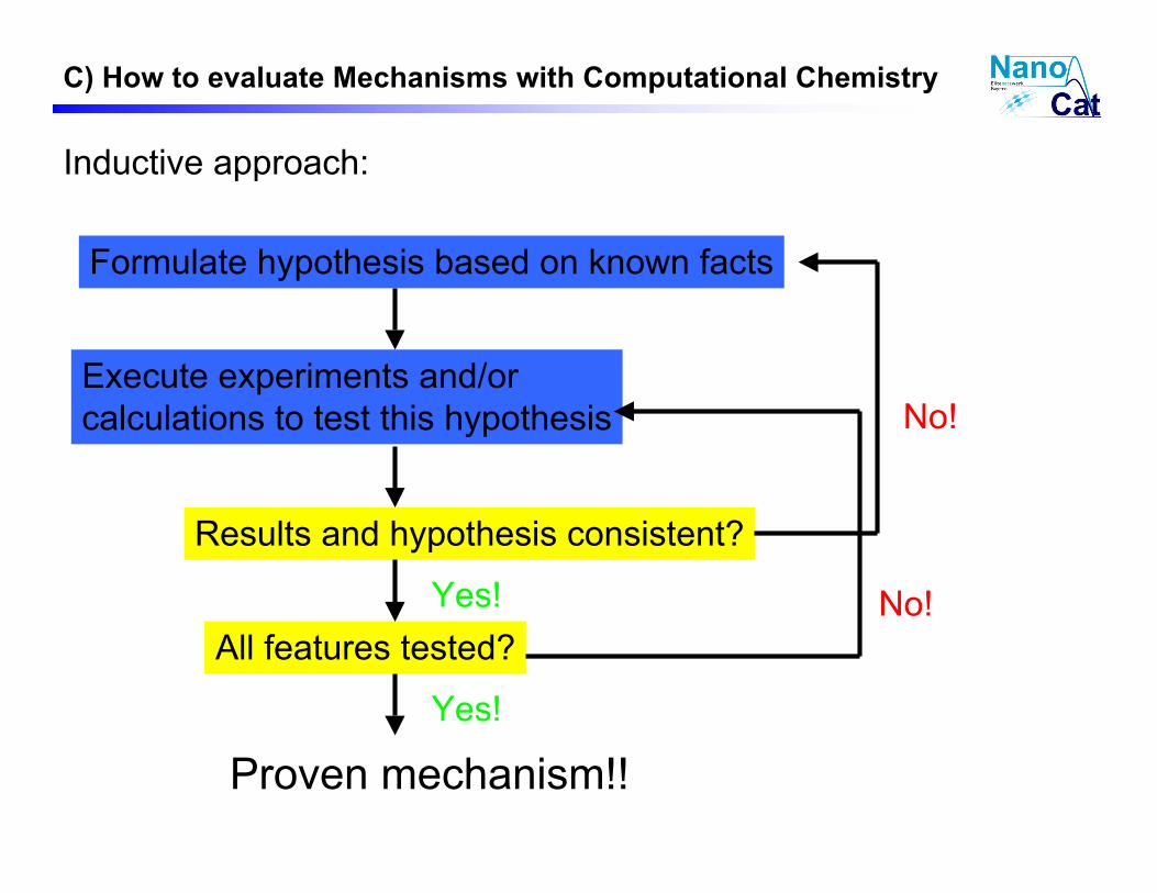
Inductive approach:
Formulate hypothesis based on known facts
Execute experiments and/or
calculations to test this hypothesis
Results and hypothesis consistent?
All features tested?
Proven mechanism!!
No!
Yes! No!
Yes!
C) How to evaluate Mechanisms with Computational Chemistry

C) How to evaluate Mechanisms with Computational Chemistry
Case study: Hydrosilylation of benzaldehyde
Possible mechanistic pathways!
Drees and Straßner, Inorg. Chem. 2007, 10850-9

C) How to evaluate Mechanisms with Computational Chemistry
How to check mechanistic pathways in computational chemistry?
1. Optimize all structures of the pathways (starting material, intermediates,
transition states, products) - be aware of isomers!
2. Frequency calculations in order to distinguish from minima structure
and transition state and to obtain the thermodynamical data
3. Choose a point on the PES to scale all the energies to (zero point).
Non-catalytic reaction: sum of reactants.
Catalytic cycle: starting point or the resting state
4. Substrate the energies of the zero-point from the energy of the desired
calculated point
5. Important: Do not loose atoms or fragments, even when compounds
are added or eliminated during the reaction!
Energy evaluation approach:

C) How to evaluate Mechanisms with Computational Chemistry

C) How to evaluate Mechanisms with Computational Chemistry
Further approaches:
- If kinetic data is available (rate constants, derived activation energies), a
comparison with the calculated barriers of the rate-determining step is
useful.
- Kinetic isotope effects could also be evaluated computationally
(=>isotope pattern at the frequency calculation!)
!
KIE = e"#G
$(D )"#G
$(H )
RT
- Simulation of spectroscopy (NMR, IR, UV) and comparison with
measurements - although with higher absolute errors than the energy
approach
derived from
!
KIE =k(H)
k(D)

C) How to evaluate Mechanisms with Computational Chemistry
Excursion: Transition states and kinetics
!
k = A " e#Ea
RT
!
k =kT
h" e
#$G
%
RT =kT
h" e
#$S
%
R " e#H
%
RT
Arrhenius equation
=> Simplest approach to calculate reaction rates or activation barriers
Transition state theory (Eyring)
=> Incorporation of the laws of thermodynamics to have access to
activation enthalpy and entropy

C) How to evaluate Mechanisms with Computational Chemistry
Meaning of the activation energies: Free energy of activation $G‡
Downside: Temperature- and concentration-dependent But: the easiest parameter for evaluation
Correlated via kinetic measurements.
A fair comparison: correlation of $G‡ with $G0 in a linear relationship.
#Example: Hammett equation
Correlation between kinetic data from a test reaction and substituent effects
!
logk
k0
"
# $
%
& ' = ()
%>0: substituent more electron withdrawing than H
%<0: substituent less electron withdrawing than H
&>0: reaction accelerated by electron withdrawing substituent
&<0: reaction accelerated by electron donating substituent
Connection to $G‡:
!
" =
#$G%
#&
'
( )
*
+ ,
#$G
#&
'
( )
*
+ ,
=
T
-.1
2.303RT/#$H%
#&

C) How to evaluate Mechanisms with Computational Chemistry
Meaning of the activation energies: Activation enthalpy $H‡
Experimental value: from the gradient in the Eyring plot (ln(k/T) vs. 1/T))
!
lnk
T
"
# $ $
%
& ' ' = (
)S*
R+ ln
k
h
"
# $ $
%
& ' ' (1
T+H
*
R
Temperature independent
#Fair comparison between theory and experiment
Interpretation as the heat that is needed to reach the reaction barrier

C) How to evaluate Mechanisms with Computational Chemistry
Meaning of the activation energies: Activation entropy $S‡
Sign of $S‡ in unimolecular reactions:
$S‡ <0 !loss of degrees of freedom in the transition state
(e.g. hydrogen transfer, cleavage of a C-X bond via HX eliminiation,
rearrangements, cyclic transition states, system crossings)
$S‡ >0 !gain of degrees of freedom in the transition state
(e.g. C-C cleavage, peroxide cleavage, biradical formations without
system crossings)

D) A Word on Costs and Accuracy Phrases of prejudice - computational costs - accuracy

D) A Word on Costs and Accuracy
„Regardless of what the experimental result would be, the computational
chemist tries to find the level of theory, where the experiment would be verified.“
(Or if the computational chemist is not your friend, but your enemy: „Regardless
of what the experimental result would be, the computational chemist tries to find
the level of theory, where the computational approach delivers a more feasible
mechanism that also fits the experimental result.“)
„Four computational chemists working on one problem would result in five
different computational results for the same experiment.“
„A computational study always needs more computational runs than initially
thought.“ (Murphy’s law for impossible time-management)
„A model system (e.g. smaller substituents) always has different behaviors
than the desired system, but saves a lot of computer time“
Well-known prejudice phrases:

D) A Word on Costs and Accuracy
Comparison of various levels of
theory in calculating the G2 test suite.
(Hundreds of molecules incl. reaction
energies)
taken from the Gaussian manual
Accuracy considerations
Level 2 // Level 1:
Geometry optimization at Level 1,
Energy calculation at level 2 for the
optimized geometry from level1.

D) A Word on Costs and Accuracy
Cost considerations
CPU = computer time
Memory = RAM memory
Disk = Disk space needed
Direct: solve integrals in the memory without storing data on the hard disk
Conventional: solve the integrals using a lot of temporary files on disk
N = number of basis sets
O = number of occupied orbitals
V = number of virtual orbitals

D) A Word on Costs and Accuracy
Cost meets accuracy
SCF Cycle for methane
SCF Cycle for pentane
The computational chemist has always to consider the need for a
specific accuracy in the focus of the higher computational costs
that this might cause.

Further reading....
Computational:
I.N. Levine - Quantum Chemistry - Prentice Hall
(broad overview)
W. Koch, M. C. Holthausen - A Chemist‘s Guide to Density Functional
Theory - Wiley-VCH
(as the name indicates, focus on DFT ,but also with a lot of physical formulas)
A. Szabo, N. S. Ostlund - Modern Quantum Chemistry: Introduction to
Advanced Electronic Structure Theory - Dover
(partly hardcore derivation of all the theory - HF and post-HF only)
Mechanisms:
B.K. Carpenter - Determination of Organic Reaction Mechanisms -
Wiley&Sons
(rather old book, focuses on kinetics and thermodynamical values)

... To be continued!
Thank you very much for your kindest attention!