development of p-y curves for piedmont residual soils · development of p-y curves for piedmont...
TRANSCRIPT
B-424 {2)
DEVELOPMENT OF P-Y CURVES FOR
PIEDMONT RESIDUAL SOILS
Prepared by
Michael Simpson, Graduate Research Assistant Dan A. Brown, Gottlieb Associate Professor of Civil Engineering
FEBRUARY 2003
DEVELOPMENT OF P-Y CURVES FOR
PIEDMONT RESIDUAL SOILS
Project No. B-424 (2)
Prepared by
Michael Simpson Dan A. Brown
Department of Civil Engineering Auburn University

ABSTRACT
DEVELOPMENT OF P-Y CURVES FOR PIEDMONT RESIDUAL SOILS
P-y curves can be used to predict a piles response to lateral loading. Computer
programs such as COM624 incorporate many p-y criteria which include: soft clay, stiff
clay below the water table, stiff clay above the water table, sand, and vuggy limestone. A
computer program can easily predict deflections and moments along the length of a pile
by using known soil strength parameters. But, there is no specific criterion for producing·
p-y curves for residual soils; therefore accurate computer solutions predicting pile
behavior to lateral loading in residual soils cannot be obtained. The behavior of residual
soils cannot be captured using these other criterion for developing p-y curves. A research
project was conducted at the Auburn University Geotechnical Test Site to create a
method to develop p-y curves for Piedmont residual soils.
Five full-scale lateral load tests and several in-situ tests to observe soil strength
were performed at the test site and analyzed. The data were used to backcalculate p-y
curves for the residual soil present at this site.
Linear p-y curves were input to COM624 until the pile deflections calculated
matched those measured in the field. The slopes of these p-y curves (k) were plotted
versus depth. A trend was observed between these k values and the in-situ soil tests
ii

performed at the site. A simple p-y relation was used to generate p-y curves by
correlating the in-situ data with the k values.
Deflections produced by COM624 were checked by comparison with the
deflections measured in the field. The deflections calculated were accurate and
conservative. The deflected shape of the pile was also similar to those observed in the
field tests.
A useful p-y criterion was developed for Piedmont residual soils. P-y curves can
be generated using data from an in-situ test performed in the residual soil. With these p-y
curves, computer programs can be used to quickly and accurately predict pile behavior
under lateral loading
iii

Style manual or journal used: ASCE Author's Guide to Journals, Books, and Reference
Publications
Computer software used: Microsoft Word, Microsoft Excel. COM624
IV

TABLE OF CONTENTS
LIST OF FIGURES ............................................................................... vii LIST OF TABLES .................................................................................. xi
1. INTRODUCTION 1.1 GENERAL .............................................................................. 1 1.2 OBJECTIVES ............................................................................ 2
2. BACKGROUND 2.1 INTRODUCTION ...................................................................... 3 2.2 P-Y METHOD ......................•.................................................... 4
2.2.1 P-Y CURVES FOR SOFT CLAY ........................................ 7 2.2.2 P-Y CURVES FOR SAND ............................................. 10 2.2.3 P-Y CURVES FOR STIFF CLAY ABOVE THE WATER
TABLE ..................................................................... 15 2.2.4 P-Y CURVES FOR STIFF CLAY BELOW THE WATER
TABLE ..................................................................... 17 2.3 PIEDMONT SOILS ................................................................... 22
2.3.1 RESIDUAL SOILFORMATION ..................................... .24 2.3.2 RESIDUAL SOIL PROFILE ........................................... .26
2.4 ENGINEERING PROPERTIES ..................................................... 28 2.4.1 STRENGTH ............................................................... 29 2.4.2 COMPRESSIBILITY .................................................... 30 2.4.3 SHRINKAGE AND EXPANSION .................................... 31 2.4.4 COMPACTION .................... ~ ..................................... 32 2.4.5 PERMEABILITY ........................................................ 32 2.4.6 GROUNDWATER ....................................................... 33
3. FIELD TEST PROGRAM 3.1 INTRODUCTION .................................................................... 34 3.2 SITE DESCRIPTION ................................................................ 34 3.3 SITE LAYOUT AND PILE PROPERTIES ...................................... .41 3.4 TEST SETUP .......................................................................... 42 3.5 TESTING PROCEDURE ........................................................... .44
4. TEST RESULTS 4.1 INTRODUCTION ..................................................................... 46 4.2 INCLINOMETER DATA .......................................................... .46 4.3 LVDT DATA .......................................................................... 47
v

4.4 STRAIN" DAT A ....................................................................... 48
5. ANALYSIS OF TEST RESULTS 5.1 IN"TRODUCTION .................................................................... 64 5.2 COMPUTATIONAL MODEL. ..................................................... 65 5.3 COM624 P-Y CRITERIA ............................................................... 67 5.4.1 DEVELOPMENT OF P-Y CURVES ............................................ 74 5.4.2 PROPOSED MODEL .............................................................. 85 5.5 P-Y CURVE RESULTS ............................................................... 85 5.6 SENSITIVITY TO EI. .............................................................. 105 5.7 SUMMARY .......................................................................... 106
6. SUMMARY AND CONCLUSIONS 6.1 SUMMARY .......................................................................... 108 6.2 CONCLUSIONS .................................................................... 108 6.3 RECOMMENDATIONS FOR FURTHER RESEARCH ..................... 109
REFERENCES .................................................................................... 110
vi

LIST OF FIGURES
Figure 2.1 Model of a pile under lateral load ................................................... .4
Figure 2.2 Conceptual p-y curve ....................................................................................... 5
Figure 2.3 Characteristic shape of the p-y curve for soft clay below the water table for
static loading ......................................................................................... 10
Figure 2.4 Characteristic shape of proposed p-y criteria for sand and static loading ...... 13
Figure 2.5 Non-dimensional coefficient B for soil resistance vs. Depth .................... 14
Figure 2.6 Characteristic shape of proposed p-y criteria for stiff clay ....................... 18
Figure 2.7 Characteristic shape of proposed p-y criteria for static loading in stiff clay ... 21
Figure 2.8 Location and idealized section of Piedmont and Blue Ridge .................... 23
Figure 2.9 Typical weathering profile of Piedmont Soil.. .................................... 25
Figure 3.1 Auburn University Test Site Plasticity Summary ................................. 36
Figure 3.2 Particle Size Distribution ...... : ........................................................ 37
Figure 3.3 Young's Modulus from DMT........................ . ........................... .38
Figure 3.4 SPT Blow Count ....................................................................... 38
Figure 3.5 PMT Modulus .......................................................................... 39
Figure 3.6 Particle Size Distribution ............................................................. .40
Figure 3.7 Auburn University Geotechnical Research Site Layout ......................... .41
Figure 3.8 Static Test Setup ...... ~ ............................................................... .43
vii
Figure 4.1 Shaft 1 Lateral Deflection vs. Depth from Inclinometer Data ................. .49
Figure 4.2 Shaft 2 Lateral Deflection vs. Depth from Inclinometer Data .................. 50
Figure 4.3 Shaft 3 Lateral Deflection vs. Depth from Inclinometer Data .................. 51
Figure 4.4 Shaft 5 Lateral Deflection vs. Depth from Inclinometer Data .................. 52
Figure 4.5 Shaft 6 Lateral Deflection vs. Depth from Inclinometer Data .................. 53
Figure 4.6 Load vs. Deflection from L VDT Data ............................................. 54
Figure 4. 7 Shaft 1 Strain Measurements at Low Loads ....................................... 55
Figure 4.8 Shaft 2 Strain Measurements at Low Loads ....................................... 56
Figure 4.9 Shaft 3 Shaft 3 Strain Measurements at Low Loads .............................. 57
Figure 4.10 Shaft 6 Strain Measurements at Low Loads ..................................... 58
Figure 4.11 Shaft 1 Strain Measurements at Increased Loads ............................... 59
Figure 4.12 Shaft 2 Strain Measurements at Increased Loads ................................. 60
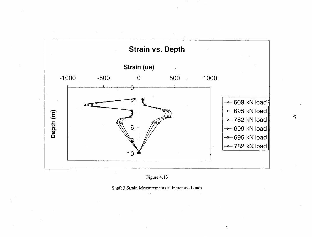
Figure 4.13 Shaft 3 Strain Measurements at Increased Loads ................................. 61
Figure 4.14 Shaft 5 Strain Measurements at Increased Loads ................................. 62
Figure 4.15 Shaft 6 Strain Measurements at Increased Loads ................................. 63
Figure 5.1 Moment vs. EI from COM624 ....................................................... 66
Figure 5.2 Load vs. Pile Head Deflection for Stiff Clay ....................................... 68
Figure 5.3 Stiff Clay Deflection vs. Depth for 569 kN Load ................................. 69
Figure 5.4 Load vs. Pile Head Deflection for Sand ............................................. 71
Figure 5.5 Sand Deflection vs. Depth for 569 kN Load ...................................... 72
Figure 5.6 Sand Deflection vs. Depth for 747 kN Load ....................................... 73
Figure 5.7 Es from Back Fit Attempt ............................................................. 75
viii
Figure 5.8 Young's Modulus from DMT ....................................................... 78
Figure 5.9 SPT Blow Count ....................................................................... 79
Figure 5.10 PMT Modulus .......................................................................... 80
Figure 5.11 Load vs. Deflection from Field Load Tests ....................................... 81
Figure 5.12 Non-linear Decrease in Soil Stiffness with Increased Deflection ............. 82
Figure 5.13 Es vs. log y/b .......................................................................... 83
Figure 5.14 Degradation Plot for Es ............................................................. 84
Figure 5.15 p-y Curve for Piedmont Residual Soil. ............................................ 84
Figure 5.16 CPT Results ........................................................................... 88
Figure 5.17 DMT Load vs. Pile Head Deflection ............................................. 89
Figure 5.18 DMT Normalized Deflection vs. Depth for 397 kN Load ..................... 90
Figure 5.19 DMT Normalized Deflection vs. Depth for 569 kN Load ...................... 91
Figure 5.20 DMT Normalized Deflection vs. Depth for 747 kN Load ...................... 92
Figure 5.21 CPT Load vs. Pile Head Deflection ............................................... 93
Figure 5.22 CPT Normalized Deflection vs. Depth for 397 kN Load ....................... 94
Figure 5.23 CPT Normalized Deflection vs. Depth for 569 kN Load ....................... 95
Figure 5.24 CPT Normalized Deflection vs. Depth for 747 kN Load ....................... 96
Figure 5.25 SPT Load vs. Pile Head Deflection ................................................. 97
Figure 5.26 SPT Normalized Deflection vs. Depth for 397 kN Load ....................... 98
Figure 5.27 SPT Normalized Deflection vs. Depth for 569 kN Load ....................... 99
Figure 5.28 SPT Normalized Deflection vs. Depth for 747 kN Load ...................... 100
Figure 5.29 PMT Load vs. Pile Head Deflection .............................................. 101
Figure 5.30 PMT Normalized Deflection vs. Depth for 397 kN Load ..................... 102
ix

Figure 5.31 PMT Normalized Deflection vs. Depth for 569 kN Load ..................... 103
Figure 5.32 PMT Normalized Deflection vs. Depth for 747 kN Load ..................... 104
Figure 5.33 Deflection vs. Depth with Varying Concrete Strength ......................... 105
x
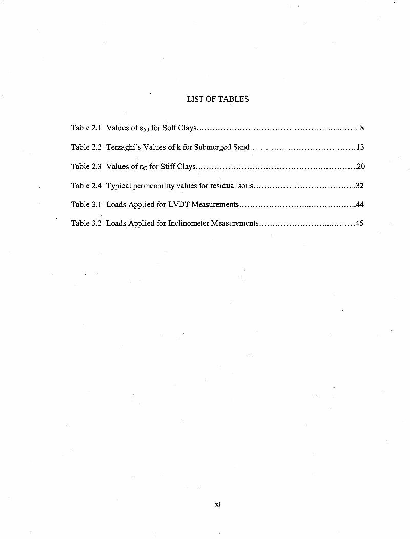
LIST OF TABLES
Table 2.1 Values of Bso for Soft Clays ............................................................. 8
Table 2.2 Terzaghi's Values ofk for Submerged Sand ....................................... 13
Table 2.3 Values of Be for Stiff Clays ............................................................ 20
Table 2.4 Typical permeability values for residual soils ...................................... 32
Table 3.1 Loads Applied for LVDT Measurements ........................................... .44
Table 3.2 Loads Applied for Inclinometer Measurements ................................... .45
xi

1.1 General
CHAPTERl
INTRODUCTION
A drilled shaft consists of a drilled hole that is filled with fluid concrete, which
can be reinforced by lowering a rebar cage into the excavation. A drilled shaft that is
sized adequately and reinforced properly can sustain large lateral loads created by earth
pressures, wind pressures, water pressures, earthquakes, impact loads, etc. Drilled shafts
are used often in the case of a large lateral load for structures such as bridges, towers, and
signs. The economic advantage of drilled shafts often occurs as a result of the fact that a
large diameter drilled shaft can be installed to replace groups of driven piles (O'Neill and
Reese, 1999).
The solution to the lateral load problem involves the pile deflection and the
reaction of the soil in which it is embedded. The deflection caused by the lateral loading
of a shaft creates reactions in the soil, where the equations of static equilibrium must be
satisfied. The problem created is a soil-structure-interaction problem, which requires
numerical relationships between the pile deflection and soil reaction. In order to
understand the pile behavior under lateral loading, some knowledge of the soil response
must be obtained. Analysis of tI:ie data from full-scale load tests provides the best means
to develop full understanding of a particular soil.
1
2
Computer programs such as FHW A COM624 are used in the analysis of laterally
loaded piles. With the input of known soil parameters, the computer program can predict
deflections and moments along the pile. This is possible because the program has p-y
criteria for certain soil types such as sand, clay above the water table, and clay below the
water table. But the program lacks a p-y criterion for Piedmont residual soils. These
soils cannot be modeled with the traditional p-y curves used in such a program. Residual
soils are weathered in-place and do not have engineering characteristics similar to
sedimentary deposits. Therefore, a criterion for developing p-y curves for Piedmont
residual soils is needed.
1.2 Objectives
The objectives of this research is as follows:
1. Six full-scale static lateral load tests were conducted in Piedmont residual soil
at the Spring Villa geotechnical test site located in Opelika, Alabama. Five of
the shafts were constructed without defects and one constructed with defects.
This research includes analysis of the data produced from the testing of the
five non-defective shafts.
2. From the analysis, recommendations for computing p-y curves for laterally
loaded piles in the piedmont residuum will be presented.

2.1 Introduction
CHAPTER2
BACKGROUND
There is not currently a design procedure for p-y curves for laterally loaded
drilled shafts in piedmont soils. Much research can be found in literature with respect to
laterally loaded piles in many different geologic settings. Yet, there is little knowledge
for geotechnical practice in piedmont residual soils. The literature on piedmont residual
soils reflects the knowledge of the geology, but the lack of research on design procedures.
There are many design methods for laterally loaded drilled shafts in soil. The p-y
method is the most widely used for the design of drilled shafts under lateral load. The p
y method solved using computers is used because of its simplicity. Four other methods
available for the solution of a single laterally loaded pile include: The elastic method,
curves and charts, static method (Broms Method), and non-dimensional curves (Reese,
1984). The elastic method and curves and charts method are not as widely used. The
elastic method is thought to have limited applications, and a large number of curves and
charts are needed for a simple case. The non-dimensional and Broms Method are a good
way to check the computer output and response of the pile. The focus of this paper will
be on the p-y method and its application to silty soils.
3
4
2.2 p-y Method
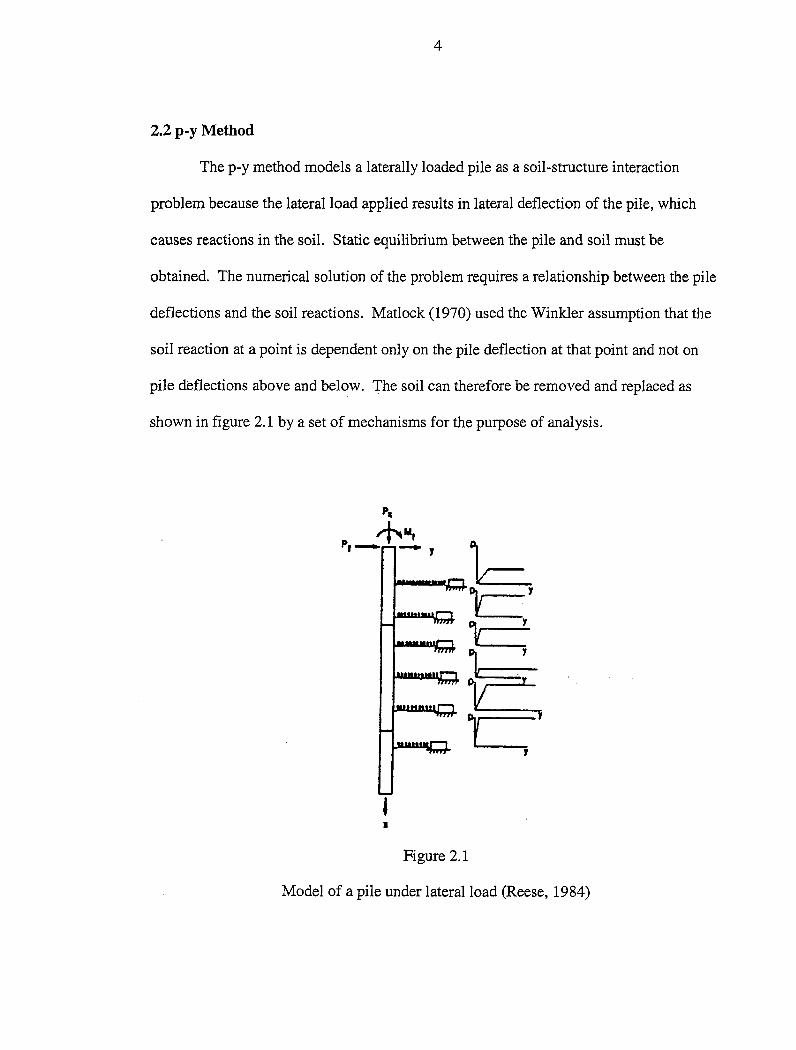
The p-y method models a laterally loaded pile as a soil-structure interaction
problem because the lateral load applied results in lateral deflection of the pile, which
causes reactions in the soil. Static equilibrium between the pile and soil must be
obtained. The numerical solution of the problem requires a relationship between the pile
deflections and the soil reactions. Matlock (1970) used the Winkler assumption that the
soil reaction at a point is dependent only on the pile deflection at that point and not on
pile deflections above and below. The soil can therefore be removed and replaced as
shown in figure 2.1 by a set of mechanisms for the purpose of analysis.
Pa
~ .. , P,_ -,
I
Figure 2.1
Model of a pile under lateral load (Reese, 1984)
5
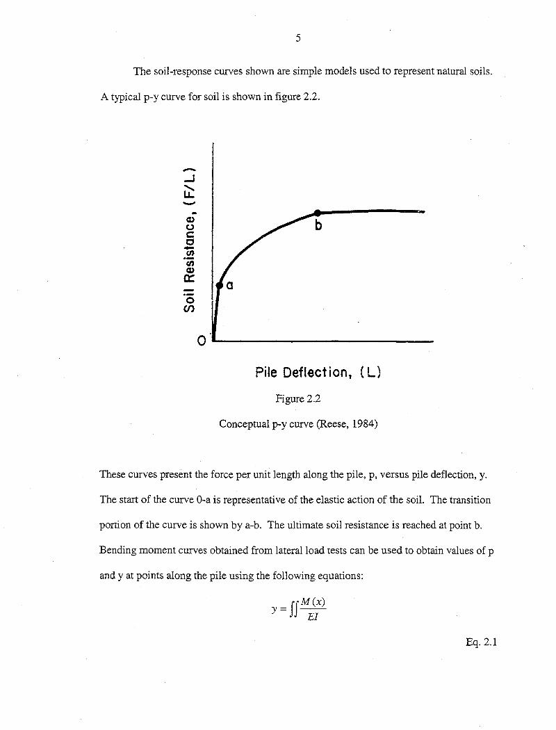
The soil-response curves shown are simple models used to represent natural soils.
A typical p-y curve for soil is shown in figure 2.2.
-_J
U: -.. a.> (.) c: c -en ·-en a.>
a::: 0 en
0
Pile Deflection, ( L)
Figure 2.2
Conceptual p-y curve (Reese, 1984)
These curves present the force per unit length along the pile, p, versus pile deflection, y.
The start of the curve 0-a is representative of the elastic action of the soil. The transition
portion of the curve is shown by a-b. The ultimate soil resistance is reached at point b.
Bending moment curves obtained from lateral load tests can be used to obtain values of p
and y at points along the pile using the following equations:
= fJM(x) y EI
Eq. 2.1

6
dz P=-M(x)
dx2
Eq.2.2
If p-y curves can be predicted, equation 2.3 can be solved to yield pile deflection, pile
rotation, bending moment, shear, and soil reaction for any load below failure.
Eq. 2.3
EI is the flexural rigidity of the pile, y is the lateral deflection of the pile at a point x
along the length of the pile, x is the position along the pile, P x is the axial load on the pile,
p is the soil reaction per unit length, and W is the distributed load along the length of the
pile (Reese, 1984). The equation can be solved using a finite difference equation 2.4
Ym-2Rm-I + Ym-/ -2Rm-1 -2Rm +Pxh2 )+ Ym(Rm-1 +4Rm +Rm+I -2Pxh 2 +kmh4
)
+ Y m+l - 2Rm - 2Rm+I + Pxh2
) + Y m+2Rm+I - Wm = 0
Eq. 2.4
where Ym is the deflection at point m along the pile, Rm is the flexural rigidity at point m,
Px is the axial load, km is the soil modulus at point m, and Wm is the distributed load at
point m. Once the deflections are obtained, the shear, moment, and slope can be found at
all points along the pile. A computer program such as FHW A COM624 is a more widely
used method of obtaining the deflections. The computer saves time and avoids human
error. This method only applies for the solution of a general case using the p-y method.
Application of the p-y method to real world problems and conditions is not as simple.
The p-y or nonlinear response method can be applied to a wide range of soil
types. Presented methods include: p-y curves for soft clay (Matlock, 1970), p-y curves

7
for sand (Reese, Cox, and Koop, 1974), p-y curves for stiff clay above the water table
(Reese and Welch, 1975), and p-y curves for stiff clay below the water table (Reese, Cox,
and Koop, 1975). These four methods cover a wide area of soil profiles.
2.2.1 p-y curves for Soft Clay
Matlock (1970) proposed a method for the development of p-y curves in soft clay.
The program was sponsored by a group of five oil companies for research on laterally
loaded piles for offshore structures in soft normally consolidated marine clay. The test
pile was 12.75 inches in diameter and embedded 42 feet. The pile was instrumented with
35 pairs of electric resistance strain gages to provide extremely accurate bending moment
measurements. The pile was driven into ciays near Lake Austin, Texas then recovered
and retested in clays in Sabine Pass, Texas.
The structural analysis of this problem is equivalent to a complex beam-column
on an inelastic foundation. The Winkler assumption allows for the separation of the soil
into several independent layers providing soil resistance p and pile deflection y.
Differentiation of the measured bending moments resulted in accurate curves of the
distribution of soil reaction along the pile. The integration of the bending moment
diagrams resulted in the deflection along the pile. Incremental loads were applied for
selected depths and p was plotted as a function of y. The recommended design procedure
was based on these experimental p-y curves.
The upper portions of the soils at Lake Austin had been subjected to desiccation
and contained joints and fissures. The Sabine clay was more typical of a slightly
overconsolidated marine deposit. Therefore the development of design criteria is based
8
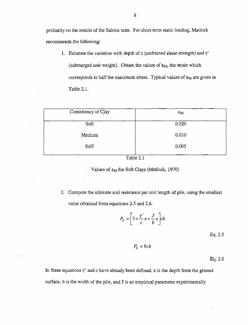
primarily on the results of the Sabine tests. For short-term static loading, Matlock
recommends the following:
1. Estimate the variation with depth of c (undrained shear strength) and y'
(submerged unit weight). Obtain the values of Eso, the strain which
corresponds to half the maximum stress. Typical values of Eso are given in
Table 2.1.
Consistency of C_lay Eso
Soft 0.020
1vledium (\(\1(\ v.V.lV
Stiff 0.005
Table 2.1
Values of Eso for Soft Clays (Matlock, 1970)
2. Compute the ultimate soil resistance per unit length of pile, using the smallest
value obtained from equations 2.5 and 2.6.
Eq. 2.5
Pu= 9cb
Eq. 2.6
In these equations y' and c have already been defined, x is the depth from the ground
surface, b is the width of the pile, and J is an empirical parameter experimentally

9
determined to be 0.5 for soft clays and 0.25 for medium clays. Using these equations the
value of Pu is calculated at each depth a p-y curve is needed.
3. Obtain y50, the deflection at half the ultimate soil resistance using equation 2. 7.
Eq. 2.7
4. Calculate the points for the p-y curve using equation 2.8. The value of p
remains constant once the value of y = 8y50 is reached.
I
P -o 5( Y ]3
-- -Pu Yso
Eq.2.8
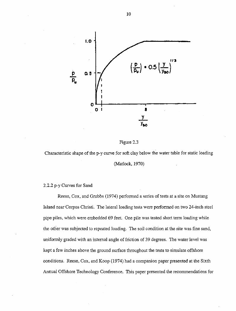
Matlock developed a procedure for obtaining p-y curves for cyclic loading, which will
not be discussed. Figure 2.3 shows a p-y curve for short-term static loading using
Matlock' s procedure for soft clay below the water table.
10
1.0
HJ
p o. e {-G;) • os l-!;) -
QL-.~----~------..,.---------...------
0 I
y -Ye.o
Figure 2.3
Characteristic shape of the p-y curve for soft clay below the water table for static loading
(Matlock, 1970)
2.2.2 p-y Curves for Sand
Reese, Cox, and Grubbs (1974) performed a series of tests at a site on Mustang
Island near Corpus Christi. The lateral loading tests were performed on two 24-inch steel
pipe piles, which were embedded 69 feet. One pile was tested short term loading while
the other was subjected to repeated loading. The soil condition at the site was fine sand,
uniformly graded with an internal angle of friction of 39 degrees. The water level was
kept a few inches above the ground surface throughout the tests to simulate offshore
conditions. Reese, Cox, and Koop (1974) had a companion paper presented at the Sixth
Annual Offshore Technology Conference. This paper presented the recommendations for

11
p-y curves in sand. Although the tests were performed in submerged sand, the tests are
applied to sands above the water table by making appropriate unit weight adjustments
depending on the position of the water table.
For both static and cyclic loading, a series of lateral loads were applied to the test
piles. Using the proper instrumentation during testing, bending moment curves were
obtained from each load applied to the piles. The bending moment curves obtained
during testing, along with the proper boundary condition for each loading type, allows for
the values of p and y to be calculated by solving equations 2.1 and 2.2. The solution of
equation 2.1 can be obtained with accurate results unlike equation 2.2. Accurate moment
measurements are required in order to solve equation 2.2 analytically.
The soil resistance curves in this study were obtained by assuming the soil
modulus could be described as a function of depth by a nonlinear curve. The parameters
for the nonlinear curve were calculated from the test data, which allowed the analytical
solution to be obtained for the soil reaction curve. Although there was some basis for this
method from theory, the empiricism involved in the recommendations was developed
because the behavior of the sand did not yield a completely rational analysis.
The ultimate soil resistance was found using free body diagrams and assuming the
Mohr-Coulomb failure theory was valid for sand. Equations 2.9 and 2.10 give the value
of ultimate soil resistance near the ground surf ace and well below the ground surf ace,
respectively.
[
_K-"-0 -,.H_t_an_</>_s_in_/3_+ tan f3 (b + H tan /3 tan o: )l ~1 = yH tan (/3 - </>)cos o: tan (/3 - </>)
+ K 0 H tan /3(tan </>sin f3 - tan o: )- Kab
Eq. 2.9

12
Eq. 2.10
In the above equations, y is the unit weight of the sand, <!> is the angle of internal friction,
b is the pile diameter, H is the depth below the ground surface, Ka is the Rankine
coefficient of minimum active earth pressure, ~ is equal to 45 + <j>/2 and is obtained from
Rankine's theory for passive pressure, a. is equal to <j>/2, and Ko is the coefficient of earth
pressure at rest. Equations 2.9 and 2.10 can be set equal to find a depth Xr. which defines
the intersection where the ultimate soil resistance near the surface and well below the
ground surface meets. Equation 2.9 should be used above this depth, and equation 2.10
below. P-y curves may be constructed at desired depths using these equations. A p-y
curve developed using this method is shown in Figure 2.4. The curve contains three
straight lines and a parabola. To yield a consistent shape between the experimental and
recommended p-y curves, the parabola and second straight line were chosen empirically.
The slope of the initial portion of the p-y curve is shown in Table 2.2.

13
x: l4
l : 13.
X: l2
p l: x,
Yu I
I I
x=O
y
Figure 2.4
Characteristic shape of proposed p-y criteria for sand and static loading (Reese, Cox, and
Koop, 1974)
Relative Density Loose Medium Dense
~ange of k (lbs/in") 2.6-7.7 7.7-26 26-51
Table 2.2
Terzaghi's Values of k for Submerged Sand (Reese, Cox, and Koop, 1974)

14
An empirical adjustment factor was needed to adjust the computed ultimate soil
resistance values for agreement with the measured values. The factor was obtained by
dividing the observed values by the computed values. The computed values were then
adjusted by this factor to obtain Pu proposed in the method. The intermediate portion of
the curve is defined by the points p and y corresponding to k, m, and u in Figure 2.4. The
respective values of Ym and Yu were found to be b/60 and 3b/80. The value of Pm can be
obtained by multiplying the ultimate soil resistance (Eq. 2.9 and 2.10) by an empirical,
non-dimensional factor B shown in figure 2.5.
0 '
1.0
2.0
l
b 3.0
4.0
5.0
6.0
8
1.0 2.0
\rllcfCYCLIC) \
' I t ~ I ,
I
f > 5.0 , Be= 0.55 Bs = 0.5
Figure 2.5
Non-dimensional coefficient B for soil resistance vs. depth (Reese, Cox, and Koop, 1974)
The p-y curve is constructed by a parabola between points k and m. The parabola
intersects the origin and connects at point m with a slope equal to the slope of line from
m to u. Point k is the intersection of the parabola with the initial straight line. Beyond u
the line is horizontal. A step-by-step method to obtain the values for the parabola and
lines is given in the recommendation, but will not be discussed.

15
2.2.3 p-y curves for Stiff Clay Above the Water Table
Welch and Reese (1972) laterally tested a drilled shaft 30 inches in diameter and
42 feet long. The site tested was located in Houston, Texas. The soil at the site consisted
of 28 feet of stiff to very stiff clay red clay, 2 feet of silt and clay layers, and very stiff tan
silty clay to a depth of 42 feet. The developed criteria are for laterally loaded drilled
shafts, both static and cyclic loading, above the water table because the water table was
located at a depth of 55 feet at the time of testing. A steel pipe 10 inches in diameter was
used as the instrument pipe, which extended two feet above the ground for a total length
of 44 feet. Strain gauges were then placed at strategic points along the pile to obtain the
required measurements. Reese and Welch (1975) analyzed the data obtained to create p
y curves.
The goal in obtaining these experimental p-y curves was to solve equations 2.1
and 2.2 previously discussed. To ensure simple differentiation and integration, a
polynomial describing a truncated power series was used to describe the data. A least
squares curve-fitting technique was then employed to fit the function to the data. A
polynomial of degree seven was found to fit the data without erratic behavior. This curve
was then double integrated to obtain the deflection of the shaft as a function of depth.
The shear was obtained by differentiating the polynomial and the soil reaction was
obtained by differentiating the shear. The p-y curves were then obtained by plotting the
soil reaction and deflection at selected depths for different loads. The recommendations
were based on these p-y curves.

16
Using the value suggested by Skempton (1951) for a long strip footing, the
deflection at half the ultimate load can be found using equation 2.7 referenced in
Matlock's soft clay recommendations. Laboratory triaxial tests were run and Eso was
found to be .005 in/in and using equation 2.7, the average value of Yso was calculated to
be 0.375 in. The ultimate soil reaction was not reached at all depths since this is a deep
foundation problem, so the values of ultimate soil reaction were estimated using equation
2.11.
I
.!_ = o.5(LJ4
Pu Yso
P =Pu for y >- l6y50
Eq. 2.11
This equation was obtained from the curve formed by plotting the values of P/Pu and
y/yso. This equation is similar to the one proposed by Matlock, and the values when
compared were in reasonable agreement near the ground surface. Since this is the most
critical zone, Matlock's equations for ultimate soil resistance were adopted (Eq. 2.5 and
2.6). The only difference used in this method is that c is the average undrained shear
strength from the ground surface to depth x, instead of the undrained shear strength at the
depth x.
An assumption was made that the shape of the laboratory stress-strain curves and the
experimental p-y curves would be similar. This correlation forms equation 2.12.
( 2.5bJ 2 y= -- e 8 so
Eq. 2.12

17
With laboratory stress-strain curves, equations 2.5, 2.6, 2.7, 2.11, and 2.12 can be used to
predict p-y curves for a deep foundation in stiff clay above the water table with a given
diameter and short-term static loading. P-y curves for cyclic loading can be obtained
with the addition of extra steps to account for the effects of repeated load.
2.2.4 p-y curves for Stiff Clay Below the Water Table
Reese, Cox, and Koop (1975) presented a design method for creating p-y curves
to the Seventh Annual Offshore Technology Conference for laterally loaded piles in stiff
clay. The criterion gives recommendations for p-y curves for stiff clay below the water
table. Two-24 inch-diameter piles and one 6-inch pile 50 feet in length were driven into
stiff clay and subjected to lateral loading near Austin, Texas. These piles were tested
with short-term cyclic and static loads. The water table was maintained at a few inches
above ground during testing to simulate clay below the water table (marine conditions).
The soils at the sight consisted of stiff, preconsolidated, clays of marine origins. Some
preliminary studies of experimental p-y curves were undertaken to establish if there was a
diameter effect seen from the tests of the 6-inch and 24 inch diameter piles. The studies
were unproductive and the recommendations were based only on the 24-inch diameter
·tests.
A characteristic p-y curve for short-term cyclic loading can be seen in Figure 2.6.
The curve has an initial straight line from the origin to point 1; two parabolic sections,
from point 1 to point 2 and from point 2 to point 3; two straight lines from point 3 to
point 4 and a horizontal line beyond point 4. At low magnitudes of soil stress and strain,

c ......... Ill .0
-a.
18
STATIC
4
y, m.
Figure 2.6
Characteristic shape of proposed p-y criteria for stiff clay (Reese, Cox, and Koop, 1975)
a straight-line relationship is often observed. The slopes of the initial straight lines were
determined using equation 2.13.
E =E. s y
Eq. 2.13
Es is the initial soil modulus; p and y are the coordinates of the initial portion of the p-y
curve.
The ultimate soil resistance, near the ground surface, uses the idea of a wedge of
clay moving up and out from the pile. Several assumptions were made in order to obtain
this equation including: the cl~y has a constant shear strength over the depth H, the
wedge of soil moving up and out can be defined by three plane surfaces and a plane next
to the pile, the undrained shear strength of the clay is fully developed along the sliding
surfaces, the bottom surface of the wedge is at a 45° with the horizontal, and there is no

19
vertical force between the pile and upward-moving soil. Equation 2.14 was derived from
this simplified failure model.
Eq. 2.14
Pc is the ultimate soil resistance at depth H, Ca is the average undrained shear strength
from the surface to depth H, b is the diameter of the pile, and y' is the submerged unit
weight of soil. At a certain depth below the ground surface, the soil will fail by flowing
horizontally around the pile. Assuming that blocks of soil around the pile have failed,
equation 2.15 is developed.
Pc= llcb
Eq. 2.15
In this equation, c is the undrained shear strength at the depth for the p-y curve. The
smaller of these two values is used for the ultimate soil resistance. The ultimate soil
resistances calculated were found to be larger than the values obtained experimentally. It
was decided to adjust the ultimate soil resistance empirically by dividing the observed
ultimate soil resistance by the computed ultimate soil resistance. The observed and
computed values agree with the use of this empirical coefficient. The remainder of the p
y curve derivation uses the concept that a load deflection curve can be related to the
stress-strain curve from a laboratory specimen, which has already been discussed.
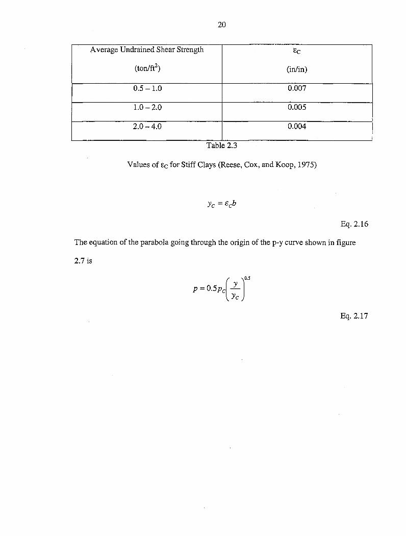
Recommendations are given for the instance when there are no laboratory stress
strain curves for the soil. Two parameters used are Ee given in table 2.3 and Ye given by
equation 2.16.
20
Average Undrained Shear Strength Ee
(ton/ft2) (in/in)
0.5 -1.0 0.007
1.0-2.0 0.005
2.0-4.0 0.004
Table 2.3
Values of Ee for Stiff Clays (Reese, Cox, and Koop, 1975)
Eq. 2.16
The equation of the parabola going through the origin of the p-y curve shown in figure
2.7 is
( J0.5
p=0.5pc ~
Eq. 2.17

21
/
/ , { y )0.5 /
p = 0.5Pc y; / ~-.....
STATIC
y-AYc 1.25 Pottset =0.055pc {-A-) Ye
~0.5pc ------ -w u 2 <{ 1-(/)
(/)
w. a:: ...J
0 (/)
0
' I I I I I I I I
:yc=E:cb I
E __ 0.0625Pc SS - Ye
6Ayc DEFLECTION, y • 1n.
Figure 2.7
Characteristic shape of proposed p-y criteria for static loading in stiff clay (Reese, Cox,
and Koop, 1975)
The parabolic shape of the p-y curve begins at the intersection the intersection of the
straight line, which starts at the origin. The parabola continues until the point defined by
the deflection Aye is reached. A is shown in figure 2.7 for the non-dimensional depth x/b
at which the p-y curve is desired. At the deflection point Aye the parabola is offset by
the value in equation 2.18.
( J!.25
y-Ay Poffset =0.055pc C
Aye
Eq. 2.18

22
At the deflection point 6Ayc, the offset stops and the p-y curve becomes a straight line
with a slope given by equation 2.19.
0.0625pc
Ye
Eq. 2.19
The straight line will continue until the deflection point of 18Ayc is reached, and then it
will become a horizontal line beyond that point. This method also allows for the
development of p-y curves for the cyclic case, which will not be discussed.
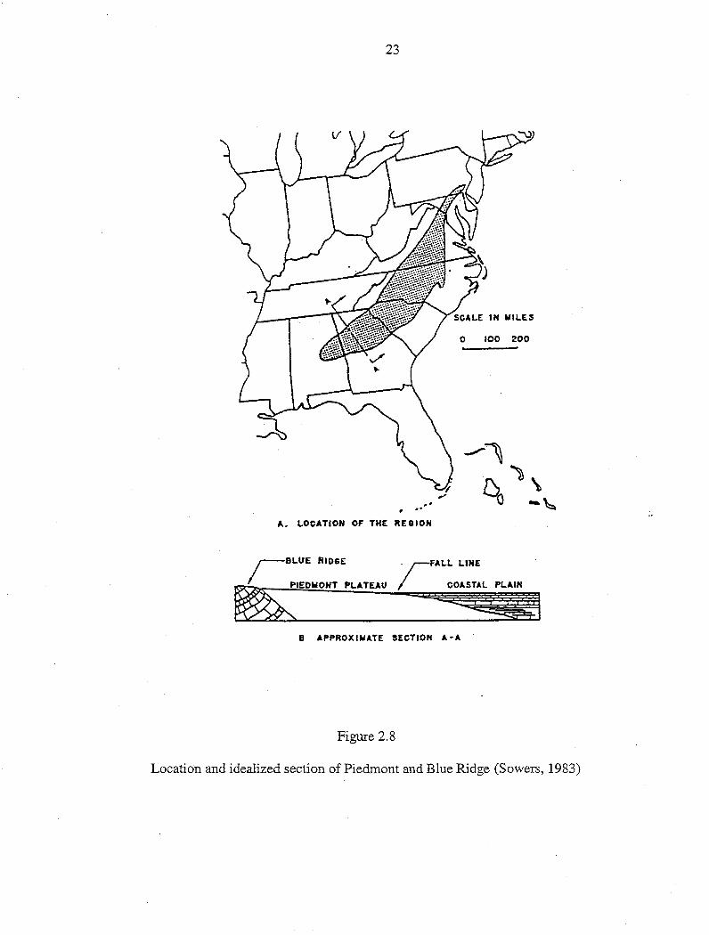
2.3 Piedmont Soils
The Piedmont consists of in-place weathered rock extending from Pennsylvania to
Alabama. It is located between the Atlantic Coastal Plain on the east and the
Appalachian Ridge on the west as shown in figure 2.8. The soil is underlain by the
parent metamorphic rock, which is predominantly composed of gneisses and schists of
early Paleozoic era or older. Intrusive deposits of granite and mafic rocks, such as
gabbro can be found. The engineering behavior of piedmont residual soil is poorly
understood (Vinson and Brown, 1997). The physical structure and engineering properties
of these soils are different from those of sedimentary materials. Since residual soils
retain much of the internal configuration (bedding and defects) of the parent rock, much
of the knowledge from the study of sediments is not applied easily to residual soils
(Sowers, 1963).
23
.. .. A. LOCATION OF THE REGION
0 100 200
/BLUE RIDGE
~IEDNDNT PLATEAU r FALl. 1.INE
COASTAL PLAIN
%Qi !@i2ilt I B APPROXIMATE SECTIOH A·A
Figure 2.8
Location and idealized section of Piedmont and Blue Ridge (Sowers, 1983)

24
2.3.1 Residual Soil Formation
The parent rocks were crystallized after being subjected to intense heat and
pressure. Once cooled, a complex fabric of interlocked mineral grains was formed.
Many of the rocks exhibit evidence of their formation under heat and pressure by the
segregation of their minerals into parallel bands or sheets (Sowers, 1963). The residual
soils are formed by the chemical decomposition of the original rock forming clay
minerals, hydrous micas, iron oxides, and semi-soluble carbonates and bicarbonates.
Mechanical weathering is not a factor because the flat topography does not promote
erosion, yet the humid climate causes rapid and deep weathering. The most important
factors affecting the depth of weathering are the composition of the. rock and the defects
such as faults and fissures (Sowers, 1954). The depth of weathering and the thickness of
the residual soil layer can be extremely variable. Due to the different degree of
weathering with depth, soil zones are formed. The weathering is greatest at shallow
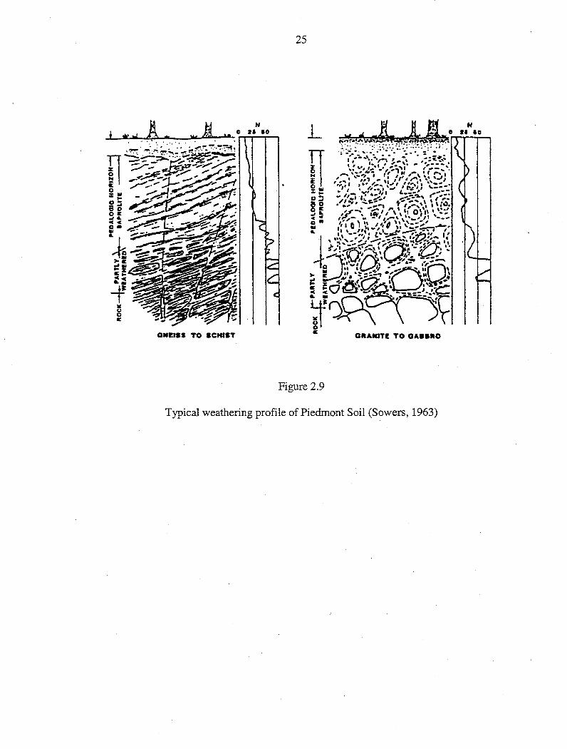
depths and decreases with depth until the parent rock is reached. The typical weathering
zones can be seen in figure 2.9.
* ... A.
GNEISS TO SCHIST
N 26 10
25
OllAICITE TO GAaattO
Figure 2.9
Typical weathering profile of Piedmont Soil (Sowers, 1963)

26
2.3 .2 Residual Soil Profile
The residual soil profile can ordinarily be divided into three zones: the upper
zone of stiff red sandy clays, the intermediate zone of loose to firm micaceous sandy silts,
and the partially weathered zone of gravelly silty sands and some rock. These three
zones are underlain by the unweathered parent rock. There is no perfectly defined
boundary for these zones because they are defined by the degree of weathering which can
be variable. There is normally a gradual transition from one zone to the other. Also, the
boundaries are not horizontal because weathering is accelerated near fractures where
water leaches. Several systems for defining the zones based on weathering have been
proposed including: Sowers (1963), Deere and Patton (1971), Brecke (1975), and Law
Engineering and Marta (1980). The major problem with any of these methods is to
define the boundaries (Sowers, 1983).
The soil of the upper zone shows little evidence of the parent rock from which
they were derived. This zone includes soil minerals such as angular quartz, small
amounts of weathered mica, clay minerals of the kaolinite family, and iron oxides. The
thickness ranges from 3 to 8 feet, but may exceed 10 feet in flat hilltops. The soils are
homogeneous and usually stiff. There are two causes for the stiffness. First, the soils are
desiccated. Since the clays are largely of the kaolinite family, they do not tend to absorb
water and swell. Second, the leaching of the soluble minerals from the surface tends to
cause the accumulation of these minerals in the deeper parts of the upper zone where they
harden into weak cements (Sowers, 1963). Due to the degree of weathering, the upper
zone contains a large amount of fines, which causes a large variability in the plasticity

27
characteristics. Liquid limits can range from 30 to 80, and plasticity indexes from 12 to
45. The soils are classified as CL or CL-:ML by the Unified Soil Classification System
(USCS).
The intermediate zone is often the most important from the foundation
engineering point of view (Sowers, 1963). Most structural foundations will be founded
in this zone because the upper zone is shallow while the intermediate zone is stronger and
deeper in comparison. The soil retains much of the characteristics of the original rock
because it is formed from the incomplete weathering of the parent rock. The soils are not
homogeneous because of the segregation of the soil minerals into bands, which resembles
the banding of the parent rock. These soils are termed saprolites because they are soil,
yet they retain the appearance and structure of the parent rock. These similarities can
include mineral alignment and defects.
The intermediate zone contains predominantly quartz, clay minerals, mica, and
partially weathered feldspars. The soil also contains oxides of iron and manganese,
which gives the soil a wide range of color. The sizes can be variable, but often are
uniform in a given area or band. The saprolite contains typical mica contents of 5 to
25%. The mica comes from the crystalline rocks, which are not as easily weathered as
the feldspars. Some soil bands may be all mica while others may contain none (Sowers,
1963). This creates a wide range of void ratios for the saprolites, because void ratios
increase with mica content. A frequency distribution curve of void ratios, based over
1,000 undisturbed samples indicates that the average void ratio is about 1 (Sowers, 1963).
The intermediate zone usually shows a grain size curve with a uniform to well
graded curve in the sand sizes, representing the unweathered quartz and mica, and a long
28
flat curve for the silt and clay sizes, representing the kaolins. Atterberg limits are not
easily obtained for the saprolite. The soil slides instead of flows in the liquid limit cup,
and the soil is not easily rolled into threads in order to determine the plastic limit. The
range of the liquid limit is approximately 25 to 60, and the plasticity indexes are much
lower from 0 to 20. The soils are J\1L and MH, according to the uses, and are described
as rnicaceous silty sands and sandy silts.
The lower limit of the intermediate zone is not well defined. Weathering becomes
less with depth, until unaltered parent rock is reached. The partially weathered zone
consists of the transition between soil and rock. The zone is characterized by lenses or
bands of relatively sound rock separated by seams of the same sandy silts and silty sands
that are found in the intermediate zone (Sowers, 1963). The lesser weathering can be
seen in grain size curves where gravel and boulder sizes are encountered. The soils are
usually non-plastic, but can be slightly plastic when small percentages of fines are
encountered. The uses classifies the partially weathered zone as GW, GF, SW, and SF.
Most can be described as slightly silty gravelly sands and silty sands (Sowers, 1954).
2.4 Engineering Properties
The engineering properties reflect the degree of weathering and the structure of
the residual soil. The properties of the upper zone resemble properties similar to
homogeneous clays. Desiccation has caused these soils to become preconsolidated and
stiff. The soils of the upper zone do not usually create engineering problems, unlike the
soils of the intermediate and partially weathered zones. These soils create engineering
problems because they are non-homogeneous in nature. This creates much variability in

29
areas such as strength, compressibility, shrinkage and expansion, compaction,
permeability, and groundwater, etc.
2.4.1 Strength
Many tests have been performed on the intermediate and partially weathered
zones including unconfined compression, direct shear, triaxial shear, rotating vane, etc.
While many tests have been made, the very complex nature of the soils makes it difficult
to draw many generalized conclusions (Sowers, 1954). Testing consistently shows the
soils exhibiting strength with no confining pressure and increasing strength with
increasing confinement. The unconfined compression test would predict very low
strength values based on this behavior. Direct shear tests are unreliable, because they
tend to over predict the strength of the soils. The triaxial shear test is the most reliable
method of testing the strength, but many samples and tests are needed to obtain accurate
results.
Many stress conditions can be modeled using various confining pressures with the
triaxial shear test. Undrained shear tests are not commonly performed for analysis of
engineering problems because of the high.permeabilities predicted. The most common
test run on the samples is the consolidated-undrained (CU) triaxial shear test. The sample
is sheared rapidly without drainage after the lateral confining pressure consolidates the
sample. The effective stresses at failure can be obtained from this test by measuring the
pore pressures in the sample. Consolidated-drained (CD) tests can be performed to
obtain the effective stresses directly but are seldom performed due to the longer testing
times.

30
The soils of the intermediate zone can be described using a two-part Mohr
Coulomb failure envelope. A straight line is observed for shearing strengths above 100
to 200 kPa, and a concave downward curve is observed at pressures below. Bonding
between the soil grains (true cohesion) can be observed. All of the physical bonds
between particles in the original rock were not broken during weathering. While soils
containing large amounts of quartz and feldspars exhibit little cohesion, soils containing
large amounts of mica exhibit much more cohesion. Part of the cohesion appears to be
the result of capillary tension since varying the moisture content (without a change in
void ratio) will change the cohesion (Sowers, 1954).
The internal friction appears to result from interlocking of angular quartz and
mica flakes plus the true friction. The increase of weathering and void ratio causes
decreases of the internal friction. Saprolites containing large amounts of mica have much
lower angles of internal friction resulting from higher void ratios.
The shear strength varies because it is anisotropic in nature. Tests with the flaky
minerals oriented parallel to the potential shear plane exhibit about two-thirds to three
fourths the strength perpendicular to it (Sowers, 1983). The strength of banded soils vary
greatly from band to band, and resemble stratified soils.
2.4.2 Compressibility
Materials of the saprolite and the partly weathered zone consolidate similar to
other soils when subjected to vertical pressures with lateral confinement. The materials
become denser with increasing confining stress. A plot of the time rate of consolidation
of a partly saturated saprolite exhibits significant initial and primary consolidation, and
31
usually significant secondary consolidation (Sowers, 1983). Higher permeabilities and
anisotropic effects of the structure of the soil on drainage causes much more rapid
primary consolidation than for clays. Secondary consolidation is often related to
structural settlement and can continue for years. More secondary consolidation can be
observed when there is a significant mica content present. The amount of secondary
settlement is relatively large, similar to that in organic soils (Sowers, 1963).
Stress-void ratio curves for saprolites resemble those for undisturbed
preconsolidated clays. Predicted preconsolidation loads using Casagrande's empirical
method, shows no correlation between depth and preconsolidation stresses. The
preconsolidation present is probably related to the residual mineral bonds of the parent
rock. When the rock cooled, the differential contraction of the various minerals caused
high stresses to develop between the grains (Sowers, 1963).
2.4.3 Shrinkage and Expansion
Most saprolite soils have very low plasticities, yet the volume changes caused by
drying and absorption of moisture sometimes resemble those of highly plastic clays.
Shrinkage and expansion appear to be mechanical processes. Shrinkage occurs when
capillary tension on the pore water compresses the soil. The soils often expand when
dried beyond the shrinkage limit caused by the loss of capillary tension in the dry voids,
which permits the quartz-mica framework to return to its original volume. Likewise, the
expansion of the soil from wettin·g reduces the capillary tension resulting in an increase in
void ratio. Unequal expansion of the soil can break the remaining mineral bonds
(Sowers, 1963).
32
2.4.4 Compaction
The clays, micaceous silts, and rnicaceous silty-sands of the upper and
intermediate zones are not easily compacted. The soils of the partly weathered zone are
good construction materials, yet they are not easily obtainable. The Standard Proctor test
(ASTMD 698-58T) shows maximum dry densities for compacted soils of the
intermediate and partially weathered zones that are lower than satisfactory for the best
fills. The optimum moisture contents vary from 12 to 35 percent. The higher values
correspond to the highly micaceous soils with lower densities. Strengths of these soils
are not as poor as expected from the low maximum densities if the compaction
percentages exceed about 95 percent of the Standard Proctor maximum (Sowers, 1963).
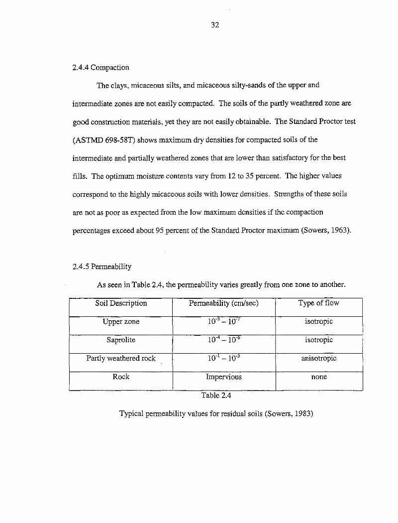
2.4.5 Permeability
As seen in Table 2.4, the permeability varies greatly from one zone to another.
Soil Description Permeability (cm/sec) Type of flow
Upper zone 10-3 -10-' isotropic
Saprolite 10-4 - 10-0 isotropic
Partly weathered rock 10-1 - 10·5 anisotropic
Rock Impervious none
Table 2.4
Typical permeability values for residual soils (Sowers, 1983)
33
The permeability is a function of the degree of weathering, the size of weather resistant
particles, and the fracture patterns. Generally, flow in the upper zone and intermediate
zone is isotropic, while flow in the partly weathered zone is anisotropic. The
permeability of the soil mass may differ greatly from the above values because of dikes
and similar intrusions of unweathered rock or seams which weather into true clays that
obstruct seepage (Sowers, 1963). The permeability is much larger parallel to foliation
than perpendicular to it.
2.4.6 Groundwater
The water levels are often complex and irregular. The normal gravity water table
is usually established in the pervious saprolite of humid regions. Within the partially
weathered zone and the rock, joints and seams form the aquifers (Sowers, 1985).
Artesian water can be found in the rock and partially weathered rock. Typically the
phreatic surface parallels the topography, but irregularities do occur from the anisotropic
permeability of the lower layers. Seasonal rainfall causes fluctuations of several meters
during the year.
3.1 Introduction
CHAPfER3
FIELD TEST PROGRAM
The Auburn University Geotechnical Site provides a facility for research on
foundation behavior in the residual soils of the Piedmont Plateau. The method of
achieving the goai of this research project was to analyze the data from full-scale lateral
load tests. Static lateral loads were applied one foot from the ground surface to six
drilled shafts. The six statically loaded piles were 36 inches in diameter, and were
embedded 36 feet into the residual soil formation. The drilled shafts in a test pair were
spaced approximately 24 feet on center. One of the shafts was purposely defected during
construction. The remaining five shafts with no defects will be discussed in this report.
3.2 Site Description
The Spring Villa Test Site lies in the Southern Piedmont Province. Specifically,
the site is located in Lee County, Alabama. The soil at the site is micaceous sandy or
clayey silt. Sand seams are also prevalent which formed from the intrusion of igneous
quartz into the metamorphic parent rock. The upper zone is approximately two to three
meters from the ground surface, underlain by the saprolite zone.
34
35
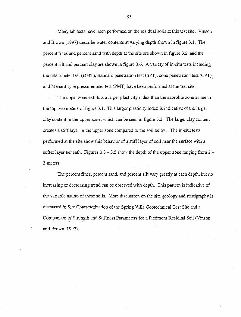
Many lab tests have been performed on the residual soils at this test site. Vinson
and Brown (1997) describe water contents at varying depth shown in figure 3.1. The
percent fines and percent sand with depth at the site are shown in figure 3.2, and the
percent silt and percent clay are shown in figure 3.6. A variety of in-situ tests including
the dilatometer test (DMT), standard penetration test (SPT), cone penetration test (CPT),
and Menard-type pressuremeter test (PMT) have been performed at the test site.
The upper zone exhibits a larger plasticity index than the saprolite zone as seen in
the top two meters of figure 3.1. This larger plasticity index is indicative of the larger
clay content in the upper zone, which can be seen in figure 3.2. The larger clay content
creates a stiff layer in the upper zone compared to the soil below. The in-situ tests
performed at the site show this behavior of a stiff layer of soil near the surface with a
softer layer beneath. Figures 3.3 - 3.5 show the depth of the upper zone ranging from 2 -
3 meters.
The percent fines, percent sand, and percent silt vary greatly at each depth, but no
·increasing or decreasing trend can be observed with depth. This pattern is indicative of
the variable nature of these soils. More discussion on the site geology and stratigraphy is
discussed in Site Characterization of the Spring Villa Geotechnical Test Site and a
Comparison of Strength and Stiffness Parameters for a Piedmont Residual Soil (Vinson
and Brown, 1997).

0
0
2
4
6
-E -.c 8 -c. Cl)
c
10
12
14
36
Water Content (0/o) 20 40 60 80
0 0 xx co x x ox 0 x
ox
ox o~o~x
0 x 0 x
~ x o Plastic Limit
x Liquid Limit
oox
0 x 0 x
ox 0 x
Figure 3.1
Auburn University Test Site Plasticity Summary (Vinson and Brown, 1997)

37
Fines(%) Sand(%)
0 50 100 0 20 40 60 80
0 0
•• •• ... •• • 2 • • 2 • •
J• • • • • -4 • • 4 • •
• • • • • • • •
6 •• •• 6 •• .. . - -E ~ • E • ~ - -.c: 8 • •• .c: 8 • • • - -c. c. Cl) Cl)
c c
10 ..... 10 • ... • • • •
12 • •• • 12 • .. -14 14
• • • • • • • •
Figure 3.2
Particle Size Distribution (Vinson and Brown, 1997)

38
Young's Modulus Derived From DMT
2
-s E -4 ..c: 15.. 5 Q)
Cl 6
7
8
9 0 1,000 2,000 3,000 4,000 5,000 6,000 7,000 8,000 9,000
Modulus (psi)
Figure 3.3
Young's Modulus from DMT (Vinson and Brown, 1997)
Average SPT N-Values
0
2
4 -E 6 -..c: -c.. 8 Q)
Cl 10
12
14 0 2 4 6 8 10 12 14 16 18 20
N-Value (blows/30cm)
Figure 3.4
SPT Blow Count (Vinson and Brown, 1997)

39
Average Modulus Derived From Pressuremeter
Modulus (psi)
0 200 400 600 800 1000 1200 1400
0
2
,..-... 4 E
6 .......... .c ......
8 0. Q)
"O 10
12
14
Figure 3.5
PMT Modulus (Vinson and Brown, 1997)

40
Silt(%) Clay(%) 0 50 100 0 10 20 30
0 0
• •• 2 2 .. • • 4 • 4 • ••• • • •
6 • 6 •
- -E •• E • • - -..r:: 8 • .c 8 •• - -a. a. Cl.) Cl.) c c
10 10
• • • •
12 • •• 12 • ... 14 14
• • ••
Figure 3.6
Particle Size Distribution (Vinson and Brown, 1997)
41
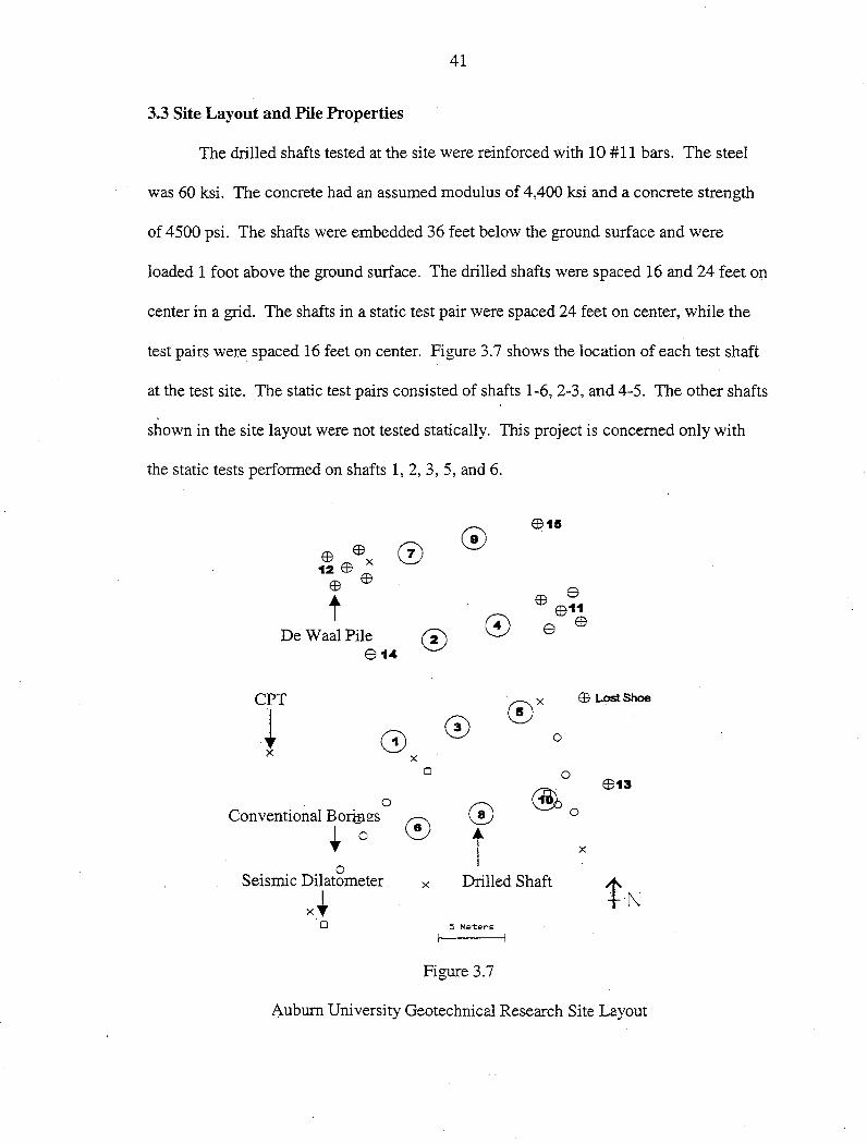
3.3 Site Layout and Pile Properties
The drilled shafts tested at the site were reinforced with 10 #11 bars. The steel
was 60 ksi. The concrete had an assumed modulus of 4,400 ksi and a concrete strength
of 4500 psi. The shafts were embedded 36 feet below the ground surface and were
loaded 1 foot above the ground surface. The drilled shafts were spaced 16 and 24 feet on
center in a grid. The shafts in a static test pair were spaced 24 feet on center, while the
test pairs were spaced 16 feet on center. Figure 3.7 shows the location of each test shaft
at the test site. The static test pairs consisted of shafts 1-6, 2-3, and 4-5. The other shafts
shown in the site layout were not tested statically. This project is concerned only with
the static tests performed on shafts 1, 2, 3, 5, and 6.
E9 E9 x 0 12 ffi
EB ffi
t De Waal Pile 0 El7 14
CPT
.i x 0
0 Conventional BorjpQ:s
t 0
x 0
(!)
0
E915
ffi E9 EJ711
El7 El7
67 Lost Shoe
0
0 $13
® 0
x
0 Seismic Dilatometer x Drilled Shaft
xt 0 5 Meters
Figure 3.7
Auburn University Geotechnical Research Site Layout

42
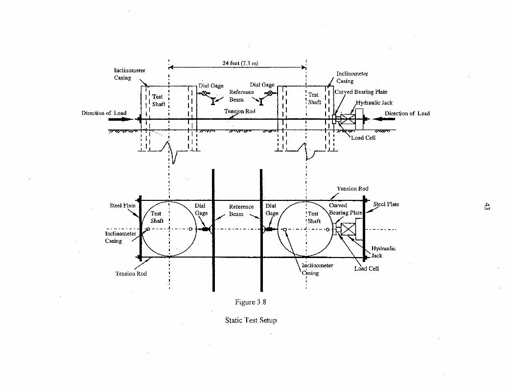
3.4 Test Setup
The instrumentation used in the test setup for this research project allows for
accurate measurements of the shaft deflections. An inclinometer tube was placed into
each shaft during construction. During testing, an inclinometer probe was lowered into
this tube to measure the deflection along the shaft. Strain gages were attached to the
reinforcement cage during construction. Gages were placed on two sides of the shaft that
correspond to the compressive and tensile zones during lateral loading. Bending
moments were monitored by placing the gages at strategic points along the pile: Between
the two shafts were located two stable reference beams, which were used in the
measurement of pile head deflections. The measurements were taken by two Linear
Variable Differential Transformers (LVDT), which were attached to these beams. Two
tension bars were connected to two beams with bolts on the outside of the test shafts.
The purpose of the tension bars was to pull the test shafts together when a load from a
jack was applied. A jack, load cell, and bearing plate were placed between one of the
shafts and the beam located on the outside of that shaft. Figure 3.8 shows the location of
the instruments. The jack was located between the load cell and the beam. The bearing
plate would be located against the shaft, and the load cell in the middle of the two. The
load cell was used to record the load being applied by the jack. The bearing plate was
used to keep the loading only in a lateral direction and relieve any twisting or torsion
caused by the loading method.
Inclinometer Casing
Casing
I I 1-· ····. ; I I I
:11~·,1: ...LJ i J......L
I
I
Tension Rod
24 feet (7 .3 m)
Dial Gage ..-.....---'----~#-. Reference Beam
I I I 11 , 11 I
Inclinometer Casing
·1~._1• ..J.....: ~ J-L
Reference Beam
Dial
Figure 3.8
Static Test Setup
Tension Rod
Oising I

44
3.5 Testing Procedure
Four of the six shafts were loaded similarly. One of the non-defective shafts was
loaded differently because higher loads were needed to fail the defective shaft, which was
being tested against it. More data was recorded for the head deflection because less time
was needed in the testing procedure.
More L VDT measurements were taken than any other measurements during the
tests. The tests only required approximately 5 minutes for each loading. After a load was
applied, the pile was observed. The L VDT measurements were taken after the pile came
to a constant displacement. Once the measurement was taken, the next load would be
applied. Table 3.1 shows the loads applied to each shaft.
Shaft Number Load (kN)
1,2,3,6 87, 174,261,348,435,522,609,
695,782
5 162,334,506,589,67, 757,870,
924
Table 3.1
Loads Applied for L VDT Measurements
Obtaining inclinometer data required more time. The process was very similar as
for the L VDT measurements. A load was applied, and the measurements were taken
45
once the constant deflection was observed. The inclinometer device had to be lowered
the length of the shaft to record all the needed data. Inclinometer data was recorded
every 0.5 m along the shaft, starting 0.5 m below the ground surface. Approximately 30
minutes was needed for the collection of data at each load interval. Due to the time
involved, not as many loadings were observed for each shaft. Table 3.2 shows the
loadings for each shaft.
Shaft Number Load (kN)
1, 6 174,348,522,695
2,3 348,435,522,609,695, 782
5 162,334,506,589,670, 757, 870,924
Table 3.2
Loads Applied for Inclinometer Measurements
Strain data were continuously monitored for each pile to determine the depth at
which the maximum bending moment occurred. The strain measurements were taken at
approximately I.Sm, 2.5 m, 3.5 m, 4.5 m, and lOm. The upper portion of the drilled shaft
is where the largest strain will occur, so this is the area observed. The strain will
decrease greatly with depth. From the strain data, the point when the concrete begins
cracking can be observed. This is the point when the compressive strains become less
than the tensile strains. The strains can be monitored to observe the location of the
maximum bending moment also. The maximum bending moment ocurrs at the location
of maximum strain.

4.1 Introduction
CHAPTER4
TEST RESULTS
The results from the static load tests of the five non-defective shafts are presented
in this chapter. The pile head deflections caused by each load were measured using a
L VDT. Inclinometer data was used to calculate the deflection along the pile for each
loading. Strain measurements were taken to observe where the .maximum bending
moment occurred in each pile, and the load when the concrete begins cracking.
4.2 Inclinometer Data
Inclinometer data from the load tests was used in Microsoft Excel to obtain
calculated deflections along the pile. Inclinometer data was taken for each shaft before
any loading was applied. These data were compared to the data taken while loads were
applied. The comparison of this data was used to obtain a plot of the deflected shape of
the pile. Inclinometer data was obtained every 0.5 meters along the pile, starting at 0.5
meters below the top of the shaft. L VDT measurements were taken to determine the
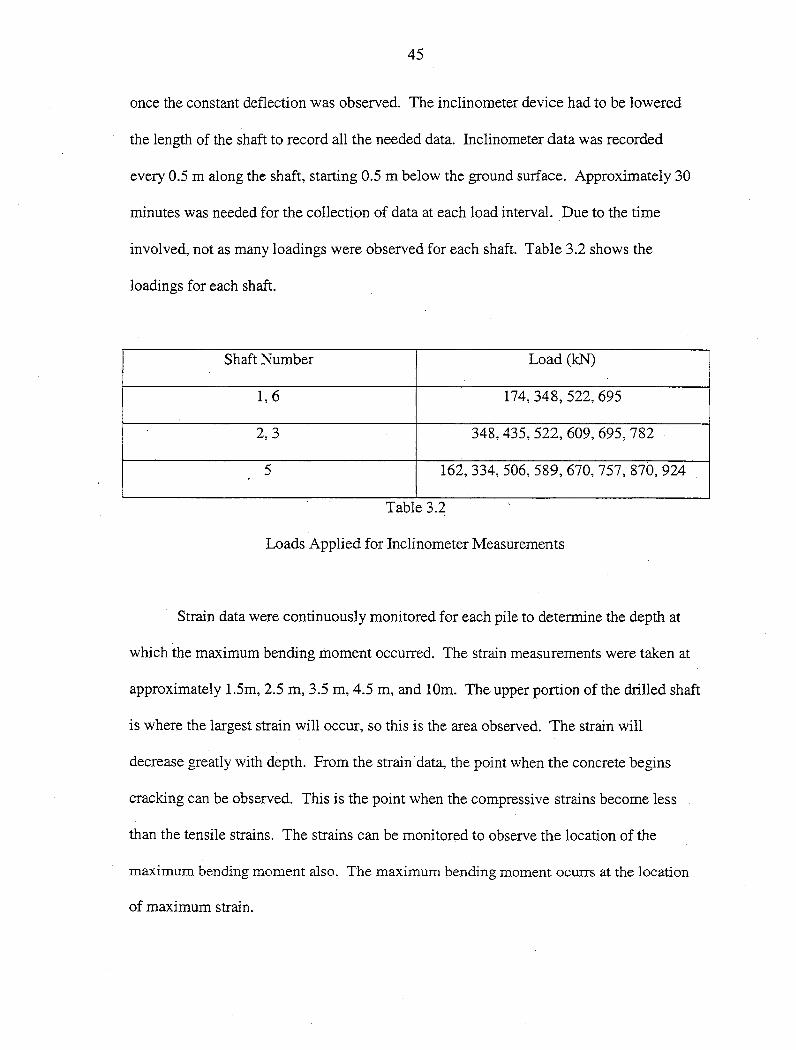
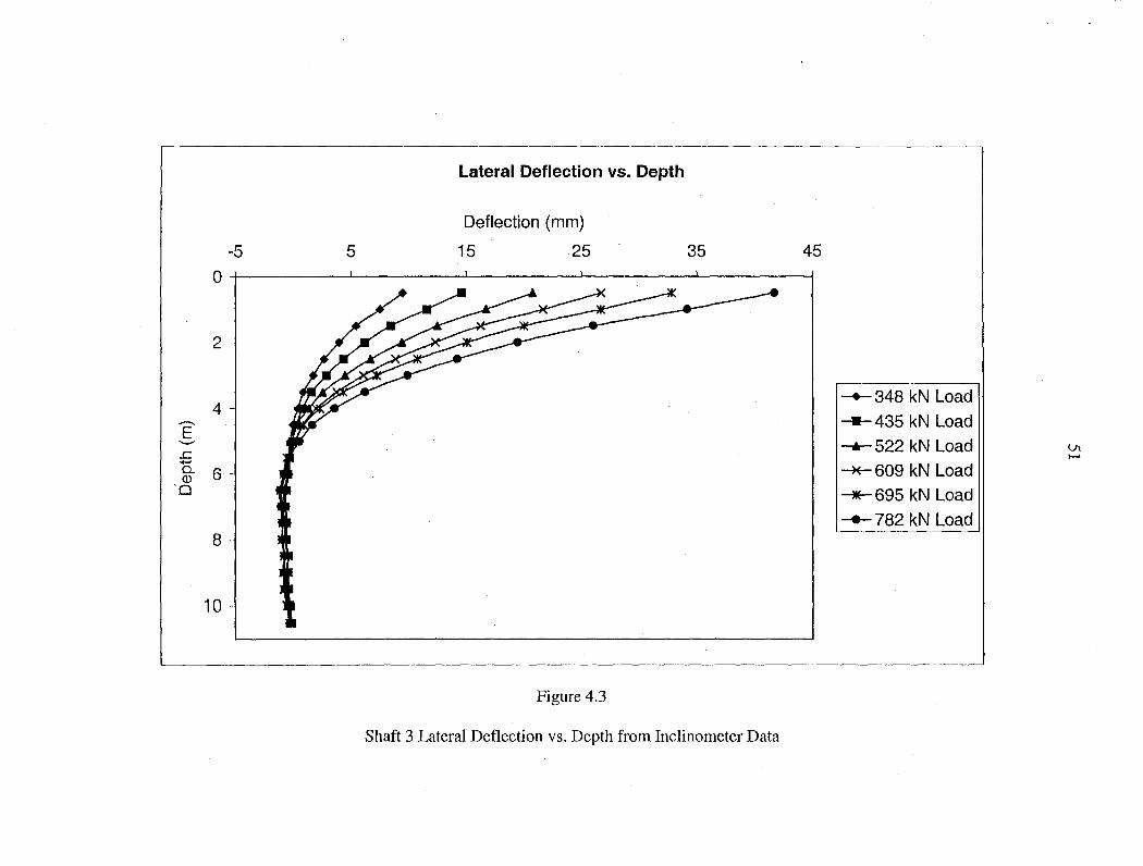
deflections at the pile head. Figures 4.1 - 4.5 shows the deflected shape of each pile for
all loads applied and recorded.
46

47
Test pair 1 - 6 had similar deflections around 35 mm for the highest load of 695
kN. The test pair displayed much different deflections for the lower loadings. Shaft 1
displayed larger deflections than shaft 6 for all other loads applied as shown in figures 4.1
and 4.5. Test pair 2 - 3 displayed a large difference in the deflections calculated for each
load. Shaft 3 experienced a deflection of approximately 42 mm near the ground surface
with an applied load of 782 kN. Shaft 2 only experienced about 29mm of deflection for
the same depth and load. Shaft 5 had a blockage in the tube and the inclinometer data
collected was incomplete; therefore a comparison of the deflections is not discussed. The
inclinometer instrument was unable to lower into the tube past a depth of around 5.5 m
below the ground surface, re.sulting in incomplete data. The problem may have been
caused by an intrusion of concrete during the casting of the shaft.
4.3 L VDT Data
The L VDT' s were used to directly measure the pile head deflection for each pile
and load. Not all the shafts were exposed to the same loadings because of the nature of
loading in pairs, discussed earlier in chapter 3. Figure 4.6 shows the results of the
measurements taken.
As expected the increase in loading causes an increase in the head deflection of
the pile. The non-linear relationship between the loaq and head deflection is shown in
figure 4.6. Shafts 1, 3, 5, and 6 reached a maximum head deflection of approximately 40
mm. Shaft 2 only reached a maximum head deflection of about 30 mm. The data exhibit
a range of behavior reflecting the variability of the response of Piedmont soils, as the
shafts were all of similar diameter and stiffness.

48
4.4 Strain Data
Strain data were continuously monitored for each pile to determine the depth at
which the maximum bending moment occurred. The strain measurements were taken at
approximately 1.5m, 2.5 m, 3.5 m, 4.5 m, and lOm. The maximum bending moment will
occur at the point along the shaft where the maximum strain occurs. This is important in
understanding where a shaft will fail.
The positive values are strains measured in the compressive zone of the loaded
pile, and the negative strains are located in the tension zone of the pile. When the tensile
strains become large the concrete will begin cracking. Once the concrete begins to crack,
the flexural rigidity (EI) will decrease significantly. Figures 4.7, 4.8, 4.9, and 4.10 show
the strain measurements at low loads for shaft 1, 2, 3, and 6. Figures 4.11, 4.12, 4.13,
4.14, and 4.15 show the strain measurements at higher loads for shafts 1, 2, 3, 5, and 6
respectively.
According to the data, the maximum bending moment occurs in the top 1/3 of
each pile, with the strain decreasing greatly with increasing depth below the ground
surface. Shafts 1 and 6 exhibit no cracking of the concrete at lower loads. The
compressive strains are similar to the tensile strains. Measurements of strains at low
loads for shaft 2 and 3 do not exhibit normal strain behavior. The compressive and
tensile strains should peak at the same depth. Therefore an error occurred in the
measurement of these values.
Shafts 1, 2, 5, and 6 clearly indicate at higher loads that the concrete is cracking.
This is indicated by large tensile strains and low compressive strains. Shaft 3 again
exhibited irregular strain behavior caused by measurement error.

Lateral Deflection vs. Depth
Deflection (mm)
-5 5 15 25 35
4 ,........ -+-174 kN Load E .........,
-348 kN Load ..c +:>. ..... \0 Q. 6 - _,.__ 522 kN Load (]) .
0 ~695 kN Load
8
Figure 4.1
Shaft l Lateral Deflection vs. Depth from Inclinometer Data

Lateral Deflection vs. Depth
Deflection (mm)
-5 5 15 25 35 45
2
-+-348 kN Load 4
-435 kN Load -E - --1s- 522 kN Load .c Ul ...... """*-- 609 kN Load
0 0.. 6 <D 0 -+- 695 kN Load
-e-782 kN Load 8
Figure 4.2
Shaft 2 Lateral Deflection vs. Depth from Inclinometer Data
Lateral Deflection vs. Depth
Deflection (mm)
-5 5 15 25 35 45 0 +-~~~~~~~~~~~~~~~~~~~~~~~~~__,
2
-+-- 348 kN Load 4
.......... -11- 435 kN Load E ..._, -...- 522 kN Load U\ .c ,_. ......
~609 kN Load a.. 6 Q) ·o _._ 695 kN Load
---- 782 kN Load 8
10
Figure 4.3
Shaft 3 Lateral Deflection vs. Depth from Inclinometer Data
Lateral Deflection vs. Depth
Deflection (mm)
-5 5 15 25 35 45
1
--+- 162 kN Load
2 - -334 kN Load ......... __..._. 506 kN Load E
............ ~589 kN Load Vt
:5 3 N a... -.- 670 kN Load ())
0 -+-- 757 kN Load 4 -+- 870 kN Load
-924 kN Load
5
Figure 4.4
Shaft 5 Lateral Deflection vs. Depth from Inclinometer Data

Lateral Deflection vs. Depth
Deflection (mm)
-5 5 15 25 35
4 -+-174 kN Load -E .._.. --348 kN Load .c ..... -..- 522 kN Load a. 6 Vl
(]) VJ 0 ~695 kN Load
8
Figure 4.5
Shaft 6 Lateral Deflection vs. Depth from Inclinometer Data

Load vs. Head Deflectiion
1 .-~~~~~~~~~~~~~~~~~~-~~~~~~~~~--.
0.9
0.8
0.7
z 0.6 ~ ::; 0.5 Ctl
.3 0.4
0.3
0.2
0.1
0 --~~~~---,~~~~~-.-~~~~~~~~~~---,~~~~~~
0 10 20 30 40 50
Deflection (mm)
Figure 4.6
Load vs. Deflection from L VDT Data
-+-shaft 1 -shaft2 _._shaft 3
~shafts
"""'*--shaft 6

Strain vs. Depth
Strain (ue)
-150 -100 -50 0 50 100
~87 kN load - -s-174 kN load E ..._. -A:- 261 kN load Vl
..s: Vl
...... --*"- 87 kN load a.
Cl)
c --.-- 261 kN load -e- 782 kN load
Figure 4.7
Shaft 1 Strain Measurements at Low Loads

Strain vs. Depth
Strain (ue)
-80 -60 -40 -20 0 20 40 60
~a7 kN load ..-.. -a-174 kN load E .._...
-&-261 kN load Vt .c: °' .....
~a7 kN load 0. Q)
c ~174 kN load ~261 kN load
Figure 4.8
Shaft 2 Strain Measurements at Low Loads

Strain vs. Depth
Strain (ue)
-100 -50 0 50 100 150
~a1 kN load - -a-174 kN load E ._.. --&-- 261 kN load Vl
J: -l ...., --"*- 87 kN load 0.
Cl> c ~ 174 kN load
-e- 261 kN load
Figure 4.9
Shaft 3 Strain Measurements at Low Loads

-100 -50
--. E -.c .. a. (I) c
Strain vs. Depth
Strain (ue)
0
Figure 4.10
50
/
Shaft 6 Strain Measurements at Low Loads
100
~a7 kN load
-s-174 kN load Ul
~261 kN load 00
-*"- 87 kN load ~174 kN load
-e- 261 kN load

Strain vs. Depth
Strain (ue)
-2000 -1500 -1 000 -500 0 500 1000
2 ~609 kN load ..-. -a- 695 kN load E ._
-tr- 782 kN load VI
.c \0
..... 6 ~609 kN load a. Q)
c ___.__ 695 kN load 8
-e- 782 kN load 10
Figure 4.11
Shaft 1 Strain Measurements at Increased Loads

-1500 -1000
..-. E .._ .c ..... c. Cl) c
Strain vs. Depth
Strain (ue)
-500
8
10
Figure 4.12
0
Shaft 2 Strain Measurements at Increased Loads
500
~609 kN load
-a- 695 kN load O'I
-o- 782 kN load 0
--*- 609 kN load
---*-- 695 kN load
-e--- 782 kN load
-1000 -500
..-.. E ._.. .c: ...... 0. C1> c
Strain vs. Depth
Strain (ue)
0
Figure 4.13
500
Shaft 3 Strain Measurements at Increased Loads
1000
-+- 609 kN load -a- 695 kN load
0\
-6- 782 kN load ~
~609 kN load
--.- 695 kN load .,--&-- 782 kN load
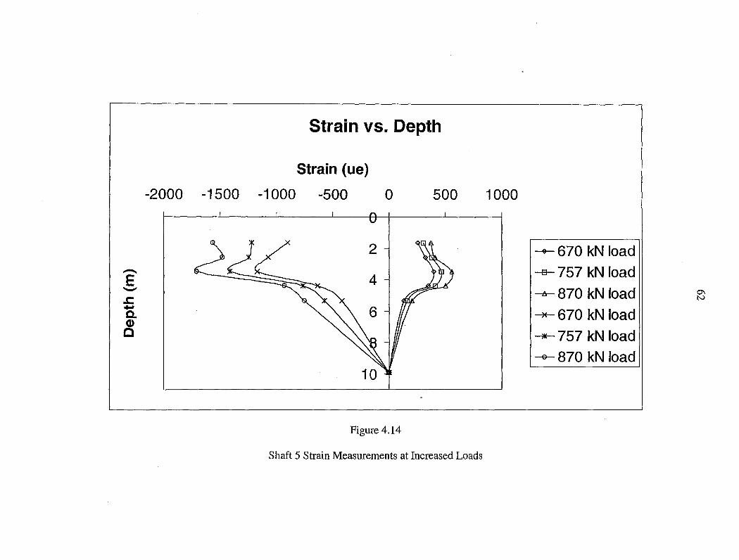
Strain vs. Dep1th
Strain (ue)
-2000 -1500 -1 000 -500 0 500 1000
~670 kN load ...-.. -a- 757 kN load E ._..
-A- 870 kN load O'I
.c N .... -x- 670 kN load Q.
Q)
c ~1s1 kN load
-a- 870 kN load
Figure 4.14
Shaft 5 Strain Measurements at Increased Loads

.-. E .._ ..c: ..... a. Cl> c
Strain vs. Depth
Strain (ue)
-2500 -2000 -1500 -1000 -500
Figure 4.15
0 500 1000
Shaft 6 Strain Measurements at Increased Loads
--+--- 609 kN load -e- 695 kN load
--&- 782 kN load 0\ l>.)
~609 kN load ~695 kN load
~782 kN load
5.1 Introduction
CHAPTERS
ANALYSIS OF TEST RESULTS
The main objective of this research project was to give recommendations for
developing p-y curves for laterally loaded shafts founded in Piedmont soils. Equations
for the development of p-y curves are presented in this chapter. The equations presented
are based on any one of the following in-situ tests in the residual soil:
1. A Dilatometer Test (DMT) with the corresponding modulus CEoMT) in psi.
2. A Cone Penetration Test (CPT) with the corresponding tip resistance (qc) in
Kpa.
3. A Standard Penetration Test (SPT) with the uncorrected blow count (N) for 30
cm.
4. A Pressuremeter Test (PMT) with the corresponding modulus CEPMT) in psi.
Using the equations presented in this chapter, p-y curves can be derived to determine
moments and deflections along the pile. This is easily accomplished using a computer
program such as COM624.
64
65
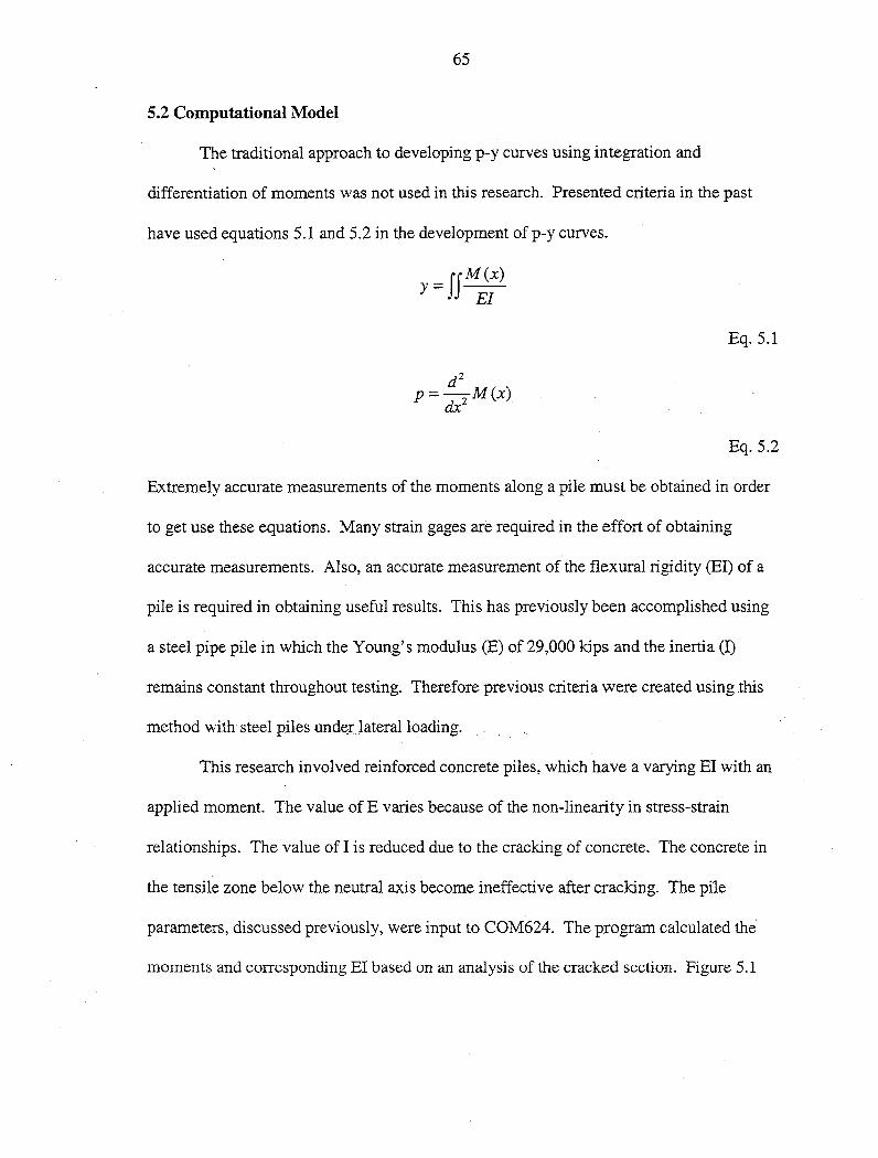
5.2 Computational Model
The traditional approach to developing p-y curves using integration and
differentiation of moments was not used in this research. Presented criteria in the past
have used equations 5.1 and 5.2 in the development of p-y curves.
= ffM(x) y EI
dz p=-
2M(x)
dx
Eq. 5.1
Eq. 5.2
Extremely accurate measurements of the moments along a pile must be obtained in order
to get use these equations. Many strain gages are required in the effort of obtaining
accurate measurements. Also, an accurate measurement of the flexural rigidity (EI) of a
pile is required in obtaining useful results. This has previously been accomplished using
a steel pipe pile in which the Young's modulus (E) of 29,000 kips and the inertia (I)
remains constant throughout testing. Therefore previous criteria were created using this
method with steel piles under.lateral loading.
This research involved reinforced concrete piles, which have a varying EI with an
applied moment. The value of E varies because of the non-linearity in stress-strain
relationships. The value of I is reduced due to the cracking of concrete. The concrete in
the tensile zone below the neutral axis become ineffective after cracking. The pile
parameters, discussed previously, were input to COM624. The program calculated the
moments and corresponding EI based on an analysis of the cracked section. Figure 5.1

66
shows the variation of EI with moment. A p-y analysis for a reinforced concrete pile will
have some computational error resulting from the assumption of a constant EI.
Moment vs. El
4.0E+OS -.----------------------.
-3.5E+08
3.0E+OS
NC 2.5E+08 ., .S- 2.0E+OS ~
- 1 C::C:,f'\O W .v1--r-vu
1.0E+OS
5.0E+07
O.OE+OO --------..,..-------.-----~
0 5000 10000 15000 Moment (in-kip)
Figure 5.1
Moment vs. EI from COM624

67
5.3 COM624 p-y Criteria
COM624 has p-y criteria built into the program, which are used to internally
generate p-y curves and allows the user to simply input soil strength parameters. These
criteria include soft clay, stiff clay below the water table, stiff clay above the water table,
sand, and vuggy limestone. The stiff clay and sand criteria were used to try and match
the deflections measured in the field. The results show that these p-y criteria lack the
capability to predict pile response in residual soils.
Three loads of 397 kN (69,000 lbs), 569 kN (128,000 lbs), and 747 kN (168,000
lbs) were input into the program. For the stiff clay criteria, the undrained shear strength
of 92 kPa (1922 psf) observed from field measurements was input and run. The results
were an extreme over prediction of head deflection; therefore these plots are not shown.
The undrained shear strength and stiffness parameters were adjusted until the head
deflection caused by the 569 kN load matched those measured in the field. The 397 kN
load predicted a pile head deflection lower than those from field tests, shown in figure
5.2. The 747 kN load caused an error to occur in the program from an excessive head
deflection. Although the 569 kN load did match the head deflection, the shape of the
deflected pile was not matched, which can be observed in figure 5.3. These results
suggest that the p-y response of the soil at this site is not well represented by curves
produced using the stiff clay criteria.

0.8
z 0.6 ~ ...._. "'O a:! .3 0.4
0.2
0 10
Load vs. Head Deflectiion
20 30 40 50
Deflection (mm)
Figure 5.2
Load vs. Pile Head Deflection for Stiff Clay
60 70
• shaft 1
• shaft 2
• shaft 3 >< shaft 5
* shaft 6 --0- C624
0\ 00
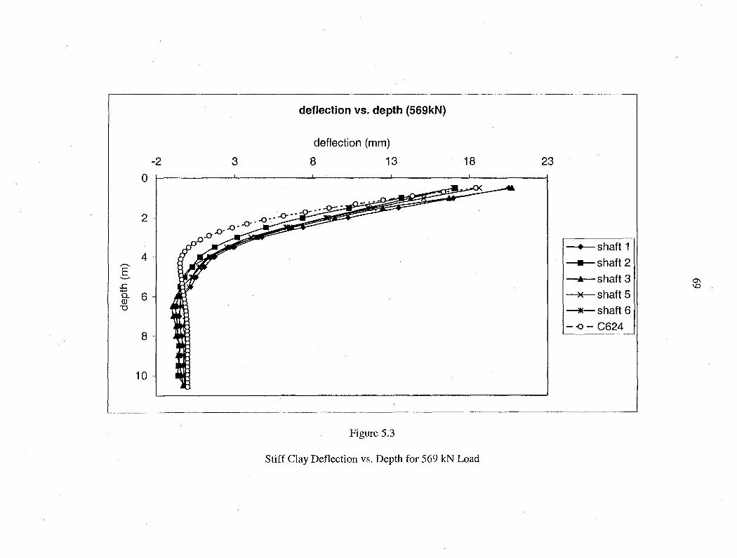
deflection vs. depth (569kN)
deflection (mm)
-2 3 8 13 18 23 0 -I-~~~~--'-~~~~~-'-~~~~~-'--~~~~--'-~~~~~~
2 .() .. ..()- .. .()•.
_{)· .{) . .0.0
• shaft 1 4 • shaft 2 ..........
E shaft 3 ..._.. ... 0\
..c \0 ...... )( shaft 5 Q. 6 -
Q) "O )I( shaft 6
- -0- C624 8
10
Figure 5.3
Stiff Clay Deflection vs. Depth for 569 kN Load

70
The angle of internal friction measured at the site (32°) was input to COM624 using sand
criteria to try and predict pile response similar to that measured in the field. Again the
pile head deflections were over predicted with a large amount of error. The angle and k
were then adjusted similarly to the undrained shear strength for stiff clay until the head
deflections from the 569 kN load matched those from the field tests. Figure 5.4 shows
the similarity in pile head deflection with the field measurements for several loadings.
The 397 kN load had a similar head deflection and deflected shape. The 569 kN and 747
kN loads resulted in head deflections similar to those measured, but the shape of the
deflected piles were different. Figure 5.5 and 5.6 shows how the shape of the deflected
piles were affected by larger lateral loads.
The clay criteria over predicted head deflections at large loads, and resulted in
different deflected shapes of the piles compared to field measurements. The sand criteria
showed similar head deflections for all observed loads, but the shape of the deflected
piles from field tests was not duplicated.
This effort indicates that residual soils cannot be modeled effectively with
existing p-y criteria for stiff clay or sand. The residual soil profile at this site (which is
thought to be typical) has a stiff layer at shallow depths (discussed in chapter 2), which
was not accounted for by these other criteria. The deflected shape of the pile was not
captured very well by either criterion, which is a result of the composition of these soils.
The soils are the result of in place weathering of parent rock. Depending on the parent
rock present, different behavi~r can be observed. The soil does not behave exactly like a
stiff clay or sand, but more as a combination of the two.
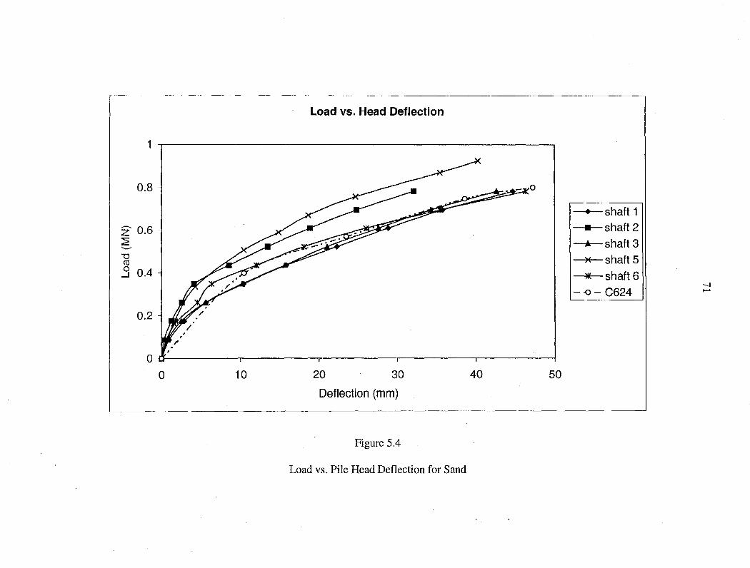
Load vs. Head Deflection
1
0.8
• shaft 1
z 0.6 • shaft 2 ~ ..__... ... shaft 3 "O )( shaft 5 co ..3 0.4 * shaft 6
-..)
- -0 - C624 ,_.
0.2
0 {J-~~~~--r~~~~~-.--~~~~---.~~~~~-.-~~~~---t
0 10 20 30 40 50
Deflection (mm)
Figure 5.4
Load vs. Pile Head Deflection for Sand

deflection vs. depth (56~1kN)
deflection (mm)
-2 3 8 13 18 23
• shaft 1 4 • shaft 2 ....-...
E shaft 3 .___... .. -.....)
..c N ..... )( shaft 5 0.. 6 Q)
\J )I( shaft 6
--0- C624 8
Figure 5.5
Sand Deflection vs. Depth for 569 kN Load
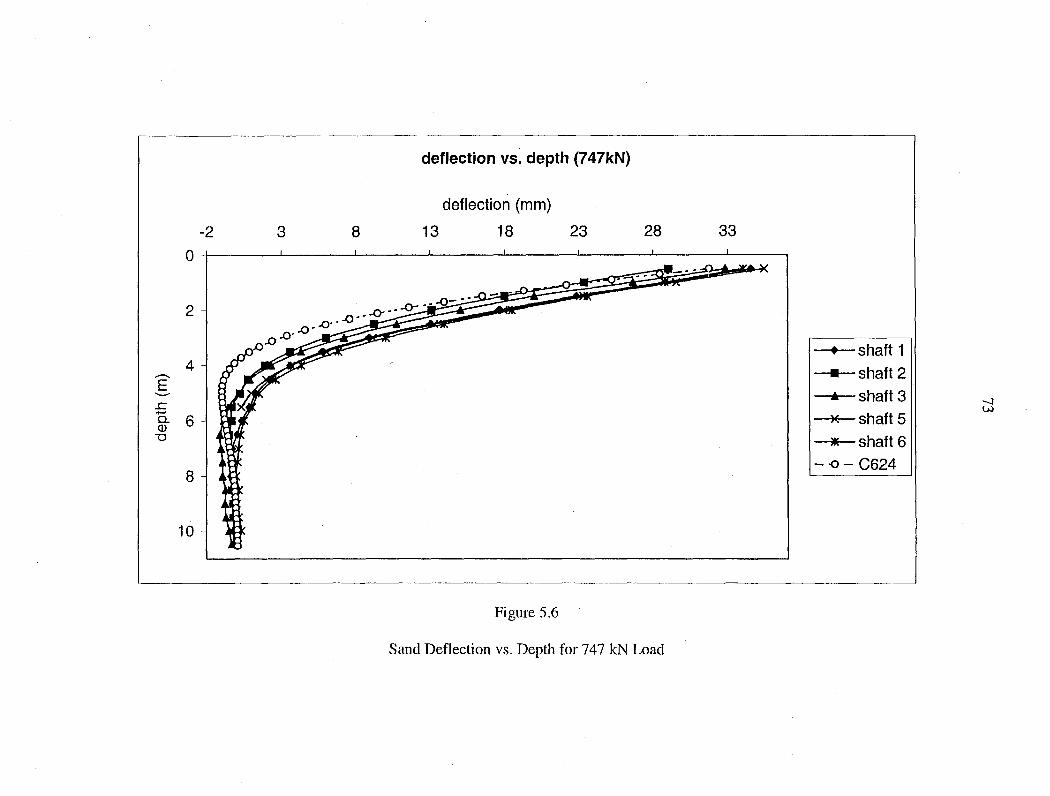
deflection vs. depth (7 47kN)
deflection (mm)
-2 3 8 13 18 23 28 33 0 -1----~~--'-~~~-L-~~~-'-~~~-'--~~--'-~~~--'-~~~-'-~~~
2
• shaft 1 4 shaft 2 -- • E
shaft 3 - • --l .c w ...... )( shaft 5 a. 6 Q)
"'O )I( shaft 6 - -0- C624
8
10
Figure 5.6
Sand Deflection vs. Depth for 747 kN Load

74
5.4.1 Development of p-y curves
In order to develop a form for p-y curves that adequately represent the Piedmont
residual soils, a simple trial and error approach was used to back fit the computer solution
to match the field measurements. Linear p-y curves were entered into COM624, which
resulted in output of deflection data along the length of the pile for each given load. The
slope of the linear p-y curves (k) was varied with depth for each load. The calculated
deflection data were compared to the data from the tested shafts, and the p-y moduli (k)
adjusted trying to match the shape of the two deflected piles.
The resulting pattern in soil stiffness is illustrated on figure 5.7. Es is defined as
k/b to establish a criterion independent of shaft diameter. The p-y relationship is
therefore:
p = (Es)(b)(y)
Eq. 5.3
In-situ data from the site were also observed and similar patterns were present, as
indicated on the plots ofDMT, SPT, and PMT test data versus depth, provided on figures
5. 8 - 5 .10. A strong correlation is observed between the lateral soil resistance on the test
shafts and the measurements of soil stiffness and strength from the in-situ tests.
The lateral soil response is softer at larger lateral displacements because the load
versus deflection showed a strong non-linearity in the lateral load versus deflection
behavior of the test shafts. This can be observed in the test shafts load versus deflection
plot shown in figure 5.11. This non-linear lateral load versus deflection is consistent with
that of other types of p-y relationships used for sands and clays. The non-linear decrease
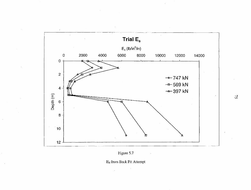
Trial E5
E5 (lb/in2/in)
0 2000 4000 6000 8000 10000 12000 14000
10
Figure 5.7
Es from Back Fit Attempt
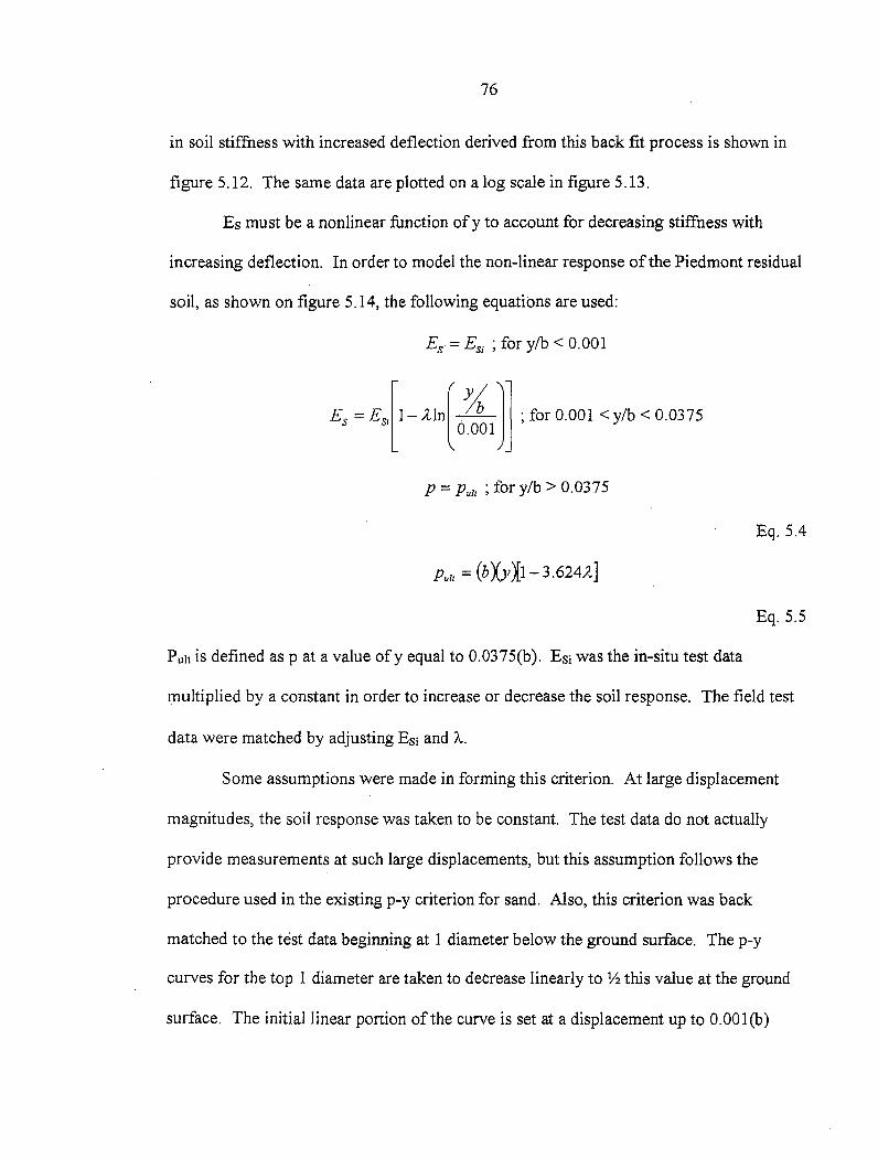
76
in soil stiffness with increased deflection derived from this back fit process is shown in
figure 5 .12. The same data are plotted on a log scale in figure 5 .13.
Es must be a nonlinear function of y to account for decreasing stiffness with
increasing deflection. In order to model the non-linear response of the Piedmont residual
soil, as shown on figure 5.14, the following equations are used:
Es =Es; ; for y/b < 0.001
E, ~ E,.11-Aln( y;; Jl ; for 0.001 < y/b < 0.0375 l 0.001 J
P = Pu1t ; for y/b > 0.0375
Eq. 5.4
Eq. 5.5
Pu11 is defined asp at a value ofy equal to 0.0375(b). Esi was the in-situ test data
multiplied by a constant in order to increase or decrease the soil response. The field test
data were matched by adjusting Esi and A.
Some assumptions were made in forming this criterion. At large displacement
magnitudes, the soil response was taken to be constant. The test data do not actually
provide measurements at such large displacements, but this assumption follows the
procedure used in the existing p-y criterion for sand. Also, this criterion was back
matched to the test data beginning at 1 diameter below the ground surface. The p-y
curves for the top 1 diameter are taken to decrease linearly to 1h this value at the ground
surface. The initial linear portion of the curve is set at a displacement up to O.OOl(b)

77
(0.1% of the shaft diameter). This cutoff is somewhat arbitrary, but it seemed to match
the test data quite well.
Using the presented recommendations; p-y curves can be constructed for
Piedmont residual soils. These p-y curves are based on in-situ test data. A constructed p
y curve in general from is shown in figure 5 .15.

2
3
-S4 .c ....... fil- 5 0
6
7
8
9
0 1,000
Young's Modulus Derived From DMT
2,000 3,000 4,000 5,000 6,000
Modulus (psi)
Figure 5.8
Young's Modulus from DMT (Vinson and Brown, 1997)
7,000 8,000 9,000
._J 00
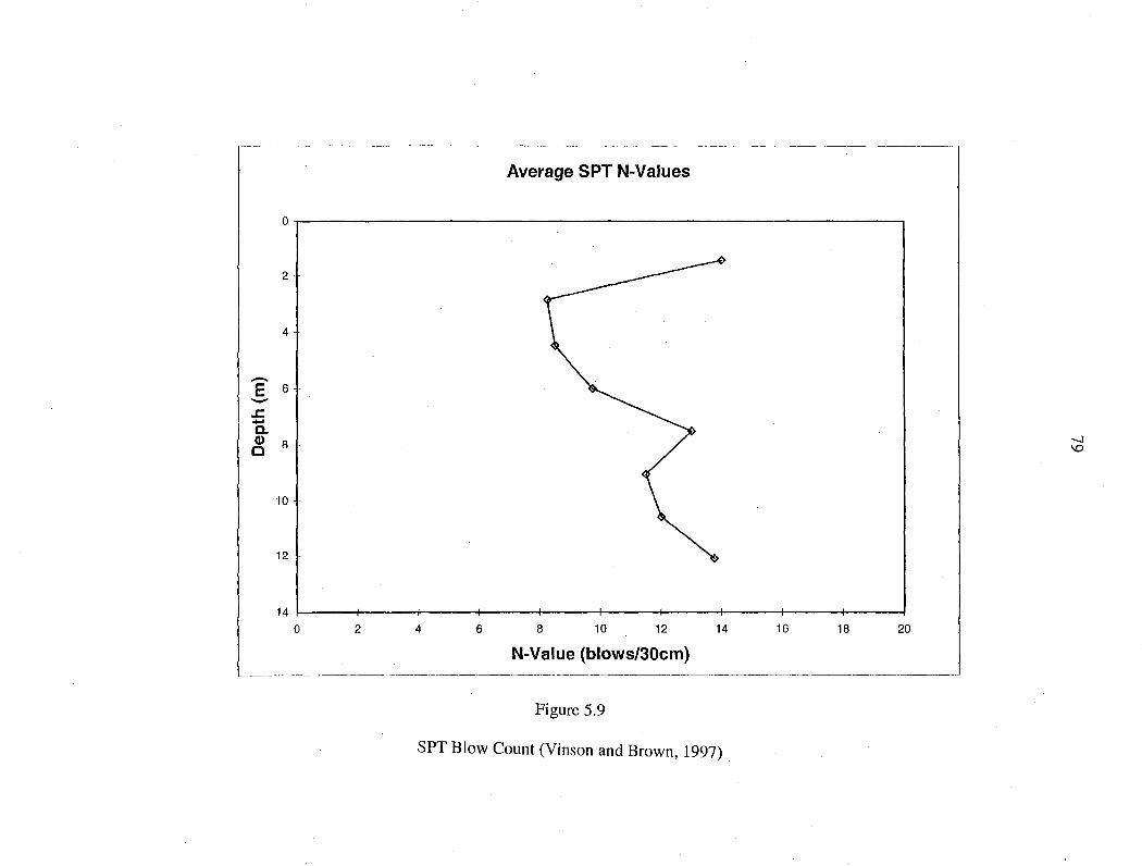
2-
4
-E 6 -.c a. Cl> 8 0
10 --
12 --
------·----------·------------ -------
Average SPT N-Values
14lo~~-+2~~-+4~~-+6~~-+a~~-+10~~-+12~~-+14~~-+16~~--+1a~~-::i20
N-Value (blows/30cm)
Figure 5.9
SPT Blow Count (Vinson and Brown, 1997) _

0
2
-.. 4 E
6 .._... ..c ..... 0.. Q)
8 "'O 10
12
14
Average Modulus Derived Fro1m Pressuremeter
Modulus (psi)
0 200 400 600 800 1000 1200
Figure 5.10
PMT Modulus (Vinson and Brown, 1997)
1400
00 0

0.9
0.8
0.7
- 0.6 z :E ; 0.5·
~ ...I 0.4
0.3
0.2.
0.1 .
Lateral Load Test Load-Deflection Data
~shaft 1
-a-shaft 2
-A-shaft 3
--e-shaft 5
~shaft 6
o-----------i-------------...... -------------------+--------*----------+-----------...... --------..... ----------+------~ 0 5 10 15 20 25 30 35 40 45 50
Deflection (mm)
Figure 5.11
Load vs. Deflection from Field Load Tests
00 .......

180 -+- depth = 1 m 160 -a- depth = 2m
...-.. 140 --&-- depth = 3m c 120 ·-~
c 100 ·-:a 80 -..._... 60 UJ w 40 00
N
20 0
0.00 0.01 0.02 0.03
y/b
Figure 5.12
Non-linear Decrease in Soil Stiffness with Increased Deflection
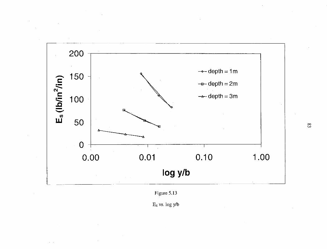
..-.. 150 -+- depth = 1 m
c: ·- -a- depth = 2m C\I .........
c: 100 ·- -tr- depth = 3m :a -.._..
fl)
w 50 00 (.).)
0
0.00 0.01 0.10 1.00
log y/b
Figure 5.13
Es vs. log y/b

1
.001
p
.001 (b)
84
In y/b
Figure5.14
Degradation Plot for Es
.0375 (b)
Figure 5.15
p-y Curve for Piedmont Residual Soil
y

85
5.4.2 Summary of Proposed Model
The proposed model was developed for Piedmont residual soils. The curve
begins as a straight line with a slope ofEsi until a deflection ofO.OOl(b) is reached.
Between a deflection of O.OOl(b) and 0.0375(b) the curve is calculated using equations
5.3 and 5.4.
p =(Es )(b)(y)
E, = E,L- ,un[ )[;. ]] ; for o. oo I < y/b < 0.03 75 l 0.001
Eq. 5.3
Eq. 5.4
The curve becomes constant after a deflection of 0.0375(b) is reached. The soil response
at this point is defined as Pu11. The value of pat this point can be calculated using
equation 5.5.
Pu1t = (bXyll-3.624A-]
Eq. 5.5
Following this model a p-y curve similar in shape to figure 5.15 can be constructed.
5.5 p-y Curve Results
Equations were developed using 4 in-situ test methods. The data from the DMT,
CPT, SPT, and PMT were used to give recommendations for developing p-y curves.
These in-situ tests were chosen because of the available data their widespread use in
geotechnical engineering.
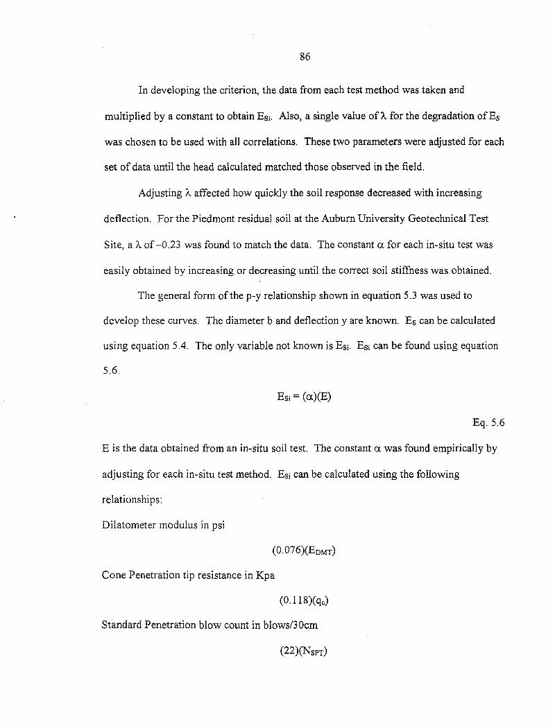
86
In developing the criterion, the data from each test method was taken and
multiplied by a constant to obtain Esi. Also, a single value of A. for the degradation of Es
was chosen to be used with all correlations. These two parameters were adjusted for each
set of data until the head calculated matched those observed in the field.
Adjusting/... affected how quickly the soil response decreased with increasing
deflection. For the Piedmont residual soil at the Auburn University Geotechnical Test
Site, a /... of -0 .23 was found to match the data. The constant a for each in-situ test was
easily obtained by increasing or decreasing until the correct soil stiffness was obtained.
The general form of the p-y relationship shown in equation 5.3 was used to
develop these curves. The diameter b and deflection y are known. Es can be calculated
using equation 5.4. The only variable not known is Esi. Esi can be found using equation
5.6.
Esi = (a)(E)
Eq. 5.6
E is the data obtained from an in-situ soil test. The constant a was found empirically by
adjusting for each in-situ test method. Esi can be calculated using the following
relationships:
Dilatometer modulus in psi
(0.076)(EDMT)
Cone Penetration tip resistance in Kpa
(0.118)(qc)
Standard Penetration blow count in blows/3 Ocm
(22)(NsPT)
87
Menard Pressuremeter modulus in psi
(0.235)(EPMT)
The data obtained from the DMT, SPT, and PMT were shown in figures 5.8, 5.9,
and 5 .10 respective I y. The CPT test data versus depth is shown in figure 5 .16. The CPT
tip resistance was used in development of the criterion because it is a better indicator of
soil strength than the other measurements. However note that the trend of higher
stiffness at shallow depth is less evident in these measurements.
Using the presented equations, p-y curves were developed to predict pile
deflections using COM624. Figures 5.17 - 5.32 provide the measured and computed
deflection data from the DMT, CPT, SPT, and PMT correlations cited above .
. All four equations produced reasonably good agreement with the measured
defl~ctions. The non-linear pile head deflections are predicted, and the deflected shapes
of the piles from the field tests were captured quite well. Shaft 2 and 5 produced lower
head deflections than the other three shafts at similar loads during testing. The equations
presented compare with the head deflections similar to shafts 1, 3, and 6. The design
equations thus fall on the conservative side with respect to the measurements.

Avg.Cone Tip
0 Resistance
2
4 ..-. E 6
'} .__. .c 8 ....., a. c) G) 10 c
~ 12
14
16 0 2000 4000 6000
qc (kPa)
Avg. Sleev1a Avg. Friction Friction Ratio
0 0
2 2
4 4 ........ ........ E E 6 6 ........ ........
.c 8 .c 8 ...... ...... a. a. G) 10 G) 10 c c
12 12
14 14
16 16 0 200 400 0 5
fs (kPa) Rr(%)
Figure 5.16
CPT Results (Vinson and Brown, 1997) .
10
00 00

DMT Load vs. Head Deflection
0.8
• shaft 1
z 0.6 • shaft 2 :E .. shaft 3 -"Cl )( shaft 5 C'O
.3 0.4 ;NE shaft 6 00
- -0 - C624 \0
0.2
0 n-~~~~-.--~~~~-,-~~~~-,-~~~~-.-~~~~~
0 10 20 30 40 50
Deflection (mm)
Figure 5.17
DMT Load vs. Head Deflection

normalized deflection vs. depth (397kN)
deflection/head deflection
-0.1 0.4 0.9
01-~-==~~1 2
• shaft 1 4 • shaft 2 - \0
E 0 - ... shaft 3 .c ....
shaft 5 c. 6 )( Cl)
'O )I( shaft 6
--o-- C624 8
10
Figure 5.18
DMT Normalized Deflection vs. Depth for 397 kN Load

--E -.c ..... a. Q)
"C
-0.1
normalized deflection vs. depth (569kN)
deflection/head deflection
0.4 0.9
0 ;---------------------:-----'--------------------------'-~=--~
2 -
4
6
8
10
Figure 5.19
DMT Normalized Deflection vs. Depth for 569 kN Load
• shaft 1
• shaft 2 \0 ~
" shaft 3 )( shaft 5 )I( shaft 6
- -0- C624

normalized deflection vs. depth i(747kN)
deflection/head deflection
-0.1 0.4 0.9 0 -I-----~~--~--------------'------------------------~~~
2
4 • shaft 1
• shaft 2 -E shaft 3 l.O - .. N ..c - )( shaft 5 a. 6 Cl)
"C )I( shaft 6 --0- C624
8
10
Figure 5.20
DMT Normalized Deflection vs. Depth for 747 kN Load

CPT Load vs. Head Deflection
0.8
• shaft 1
z 0.6 • shaft 2 ~ • shaft 3 -"C
)( shaft 5 cu 0
shaft 6 \0 ...J 0.4 )I( w
- -0- C624
0.2
o~~~~~~~~~~----.~~~~~..,.-~~~~-.-~~~~--;
0 10 20 30 40 50
Deflection (mm)
Figure 5.21
CPT Load vs. Head Deflection

-E -.c .... D. Q)
"C
4
6
8
10
normalized deflection vs. depth (397kN)
deflection/head deflection
0.4
Figure 5.22
CPT Normalized Deflection vs. Depth for 397 kN Load
0.9
• shaft 1
• shaft 2 \0 .. shaft 3 ..i::.
)( shaft 5 )I( shaft 6
--0- C624

-0.1
2
4 -E -.c .... a. 6 Q) "C
8
10
normalized deflection vs. depth (569kN)
deflection/head deflection
0.4
Figure 5.23
CPT Normalized Deflection vs. Depth for 569 kN Load
0.9
• shaft 1
• shaft 2 '° • shaft 3 Vl
)( shaft 5 )I( shaft 6
- -0- C624
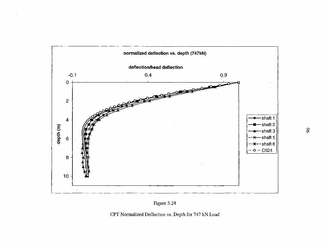
4 -E -.c .... c. 6 Q)
"O
8
10
normalized deflection vs. depth (747kN)
deflection/head deflection
0.4
Figure 5.24
CPT Normalized Deflection vs. Depth for 747 kN Load
0.9
• shaft 1
• shaft 2
'° • shaft 3 °' )( shaft 5 )I( shaft 6
--0- C624

SPT Load vs. Head Deflection
0.8
• shaft 1
z 0.6 --11- shaft 2 :::;; .. shaft 3 -"O
)( shaft 5 m 0 0.4 ...J -*-Shaft6 \0
-.)
--o-- C624
0.2
0 10 20 30 40 50
Deflection (mm)
Figure 5.25
SPT Load vs. Head Deflection

normalized deflection vs. depth (397kN)
deflection/head deflection
2
4 • shaft 1
- • shaft 2 E \0 - • shaft 3 .c 00 ....
)( shaft 5 c.. 6 Cl) "C )I( shaft 6
--0-C624 8
Figure 5.26
SPT Normalized Deflection vs. Depth for 397 kN Load

-0.1
2
4 -E -.c ..... a. 6 Q) 'O
8
normalized deflection vs. depth (569kN)
deflection/head deflection
0.4
Figure 5.27
SPT Normalized Deflection vs. Depth for 569 kN Load
0.9
shaft 1
---shaft2 \0 \0
• shaft 3
-*-shafts
---.- shaft 6
--o-- C624

normalized deflection vs. depth i(747kN)
deflection/head deflection
4 • shaft 1
- • shaft 2 E -- .. shaft 3 ..c 0 - 0 0. 6 )( shaft 5 CD "tJ )I( shaft 6
--O-C624
8
Figure 5.28
SPT Normalized Deflection vs. Depth for 747 kN Load

PMT Load vs. Head Deflection
0.8
• shaft 1
z 0.6 • shaft 2 :: .. shaft 3 -"C )( shaft 5 ca ,__. 0 0
..J 0.4 )K shaft 6 ,__.
- -0- C624
0.2
Qn-~~~~-,-~~~~--,--~~~~~~~~~--.~~~~--i
0 10 20 30 40 50
Deflection (mm)
Figure 5.29
PMT Load vs. Head Deflection

normalized deflection vs. depth (397kN)
deflection/head deflection
-0.1 0.4 0.9
2
• . shaft 1 4
shaft 2 - • ...... E 0 - • shaft 3 N .c - shaft 5 0. 6 )( Cl>
'"C lK shaft 6
--o-- C624 8
Figure 5.30
PMT Normalized Deflection vs. Depth for 397 kN Load

normalized deflection vs. depth (569kN)
deflection/head deflection
-0.1 0.4 0.9
2
--+-shaft 1 4
shaft 2 - • ...... E 0 - -.--shaft3 VJ
..c: ..... shaft 5 Q. 6 )(
Q)
"C )I( shaft 6
--o-- C624 8
Figure 5.31
PMT Normalized Deflection vs. Depth for 569 kN Load

normalized deflection vs. depth (7 47kN)
deflection/head deflection
4 • shaft 1
- • shaft 2 E - ... shaft 3
,..... 0 .c +:>. ....
)( shaft 5 a. 6 CD "C )K shaft 6
--0-C624
8
Figure 5.32
PMT Normalized Deflection vs. Depth for 747 kN Load

105
5.6 Sensitivity to EI
COM624 calculates EI based on the input concrete compressive strength ((' c).
The program calculates the initial concrete modulus as 57,000 (f c)0·5
. For this research,
the concrete strength was approximately 4500 psi. In order to evaluate the influence of
this parameter, some sensitivity tests were performed using COM624.
Presented in figure 5.33 are deflections calculated in COM624 for concrete
strengths of both 4500 and 5500 psi. The plot is the deflection versus depth produced
using the DMT equation with a 569 kN load. Notice that the deflections are almost
identical. Small differences in the measurement of concrete compressive strength do not
appear to significantly influence the computations.
-E -J: -c. (I)
c
-2.0
0
2
4
6
8
10
12
Deflection vs. Depth
Deflection (mm)
3.0 8.0 13.0 18.0
Figure 5.33
~ fc = 4500 psi
-o- fc = 5500 psi
Deflection vs. Depth with Varying Concrete Strength

106
5.7 Summary
COM624 lacks a criterion for computing p-y curves for residual soils. A
formulation has been presented which can be used to compute p-y curves based on
correlations with four types of in-situ test data developed from the Spring Villa Test Site.
Using these p-y curves, COM624 becomes a useful tool in predicting pile behavior in
Piedmont residual soils.
The presented criterion was formed using full-scale lateral load tests and in-situ
tests performed in residual soil. A simple relationship shown in equation 5.3 relates p
with k (Es = k/b) and y. A logarithmic degradation of Es was assumed to account for the
non-linear decrease in soil stiffness with increased load and deflection. The model was
adjusted to back fit the data from the test site. The equation in a general form is as
follows:
where:
p = (Es)(b )(y)
Es =Es; ; for y/b < 0.001
= EJ 1-Aln[ Jj{ ]] ; for 0.001 < y/b < 0.0375 l 0.001
P = Puu ; for y/b > 0.0375
A= -0.23
Esi = (0.076)(EoMT)

= (O. l 18)(qc)
= (22)(NsPT)
= (0.235)(EPMT)
b = diameter of pile
y = deflection
107
The results using this criterion match the data collected in the field to a degree
sufficient for design oflaterally loaded drilled shafts. The shape of the deflected pile is
captured quite well by all four equations. Also, the head deflections calculated using
these equations are conservative. Since the equations produce similar results, each one ,
should be equally useful in design.

6.1 Summary
CHAPTER6
SUMMARY AND CONCLUSIONS
Six Full-scale load tests and several in-situ tests were performed at the Auburn
University Geotechnical Research Site. The data from the in-situ tests were used to
create a criterion for developing p-y curves for Piedmont residual soils. Equations to
develop these p-y curves were formed using the DMT, CPT, SPT, and PMT. Linear p-y
curves were used in COM624 to match the deflections measured in the field tests. A
trend was observed between the in-situ data and the slope of these p-y curves. A simple
relationship, equation 5.3, was used to relate p and y. The equations were then formed by
accounting for the decrease in soil stiffness with increasing deflection, and by
incorporating the in-situ test data to form each equation. The five non-defective load
tests served as a basis for checking the accuracy of this criterion by using COM624 to
predict the deflections from these input p-y curves.
6.2 Conclusions
The objectives of this research were to analyze the load tests performed at the
Spring Villa geotechnical test site located in Opelika, Alabama and from the analysis, to
give recommendations for computing p-y curves for laterally loaded piles in the piedmont
108

109
residuum. A criterion for developing p-y curves was developed using in-situ test data
from the site. The criterion produced results which were similar to the field test data.
The results were conservative and sufficient for design of laterally loaded piles. The data
suggest that a usEful criterion has been developed for Piedmont residual soils.
6.3 Recommendations for Further Research
The following recommendations are made concerning the developed criterion for
p-y curves in Piedmont residual soils:
1. These p-y criteria need to be implemented into COM624 or LPILE using ·a
new subroutine.
2. · Additional tests need to be conducted in other areas of the Piedmont. The
residual soils in which this research was conducted lies in one localized area
of the Southern Piedmont. Different ranges of shaft diameter need to be
tested. Most important, more tests need to be performed in a range of
different soil stiffness and A-horizon thickness.
3. It is important to compare future test results with a variety of in-situ tools,
since the cross-correlations may also vary.
4. Field test data is needed for other silty soil geologic conditions similar to the
Piedmont.
There is much further research needed involving the development of p-y curves for
residual soils.
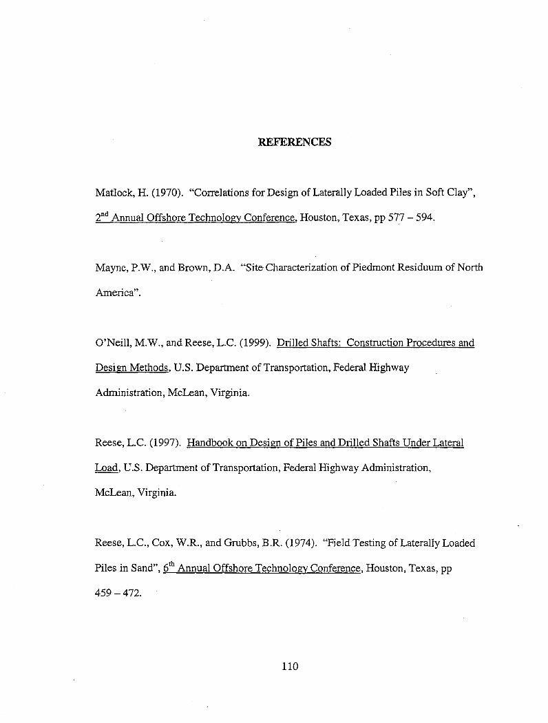
REFERENCES
Matlock, H. (1970). "Correlations for Design of Laterally Loaded Piles in Soft Clay",
2nd Annual Offshore Technology Conference, Houston, Texas, pp 577 - 594.
Mayne, P.W., and Brown, D.A. "Site Characterization of Piedmont Residuum of North
America".
O'Neill, M.W., and Reese, L.C. (1999). Drilled Shafts: Construction Procedures and
Design Methods, U.S. Department of Transportation, Federal Highway
Administration, McLean, Virginia.
Reese, L.C. (1997). Handbook on Design of Piles and Drilled Shafts Under Lateral
Load, U.S. Department of Transportation, Federal Highway Administration,
McLean, Virginia.
Reese, L.C., Cox, W.R., and Grubbs, B.R. (1974). "Field Testing of Laterally Loaded
Piles in Sand", 6th Annual Offshore Technology Conference, Houston, Texas, pp
459-472.
110

111
Reese, L.C., Cox, W.R., and Koop, F.D. (1974). "Analysis of Laterally Loaded Piles in
Sand", 6th Annual Offshore Technology Conference, Houston, Texas, pp 473 -
483.
Reese, L.C., Cox, W.R., and Koop, F.D. (1975). ''Field Testing and Analysis of
Laterally Loaded Piles in Stiff Clay", 7th Annual Offshore Technology
Conference, Houston, Texas, pp 671- 690.
Reese, L.C., and Welch, R.C. (1975). "Lateral Loading of Deep Foundations in Stiff
Clay", Journal of Geotechnical Engineering Division, 101:7, pp 633 - 649.
Robertson, P.K., and Mayne, P.W. (1998). "Geotechnical Site Characterization",
Proceedings of the First International Conference on Site Characterization,
Atlanta, Georgia, pp 1229 - 1234.
Sowers, G.F. (1954). "Soil Problems in the Southern Piedmont Region", Proceedings,
ASCE, Vol. 80, separate 416, pp 1 - 16.
Sowers, G.F. (1963). "Engineering Properties of Residual Soils Derived from Igneous
and Metamorphic Rocks", Proceedings, 2nd Pan American Conference on Soil
Mechanics and Foundation Engineering, Rio De Janeiro, Brazil, Vol. 1, pp 39- 61.

112
Sowers, G.F., and Richardson, T.L. (1983). "Residual Soils of the Piedmont and Blue
Ridge", Transportation Research Record, No. 919, Washington, D.C., pp 10- 16.
Vinson, J.L., and Brown, D.A. (1997). Site Characterization of the Spring Villa
Geotechnical Test Site and a Comparison of Strength and Stiffness Parameters for a
Piedmont Residual Soil, Auburn University Highway Research Center, Auburn,
Alabama.