development of multi-link geometry-based mimo …
TRANSCRIPT

AALTO UNIVERISTY
SCHOOL OF SCIENCE AND TECHNOLOGY
Faculty of Electronics, Communications and Automation
Department of Radio Science and Engineering
Alvaro Palacios Morales
DEVELOPMENT OF MULTI-LINK GEOMETRY-BASED MIMO CHANNEL
MODEL
Thesis submitted in partial fulfillment of the requirements for the degree of Master of
Science in Technology.
Espoo, July 31, 2010
Thesis supervisor:
Prof. Pertti Vainikainen
Thesis instructor:
Lic. Sc. (Tech.). Juho Poutanen


AALTO UNIVERSITY
SCHOOL OF SCIENCE AND TECHNOLOGY
ABSTRACT OF THE
MASTER‟S THESIS
Author: Alvaro Palacios Morales
Title: Development of multi-link geometry-based MIMO channel model
Date: 31. 06. 2010 Language: English Number of pages: 111
Faculty: Faculty of Electronics, Communications and Automation
Department: Department of Radio Science and Engineering
Supervisor: Prof. Pertti Vainikainen
Instructor: Lic. Sc. (Tech.). Juho Poutanen
Abstract:
Forthcoming wireless communication systems need larger capacity. MIMO systems are already
an answer that enables to achieve large increase to the link capacity. However, a wide and
precise knowledge of the radio propagation channel is required in order to exploit the many
benefits and capabilities of MIMO systems.
In this master‟s thesis a multi-link geometry-based MIMO channel model was developed. This
work analyses the effect of common clusters on multi-link MIMO capacity and inter-link
correlation based on simulation studies. Furthermore, the basics on radio wave propagation and
MIMO systems as well as a review on existing MIMO channel models are also provided.
Finally simulation results revealed that, in general, common clusters increase the inter-link
correlation, and so the ML-MIMO capacity decrease. But sometimes cluster geometry together
with array geometry fully determines the MIMO system performance independently of the
significance of common clusters. In addition, it was shown how often the overall system
performance is degraded. Finally, it was also investigated that a common cluster which is really
significant for only one link is not in fact a common cluster.
Keywords: MIMO, common cluster, dual-link capacity, inter-link correlation, geometry-based
channel model, Multi-Link channel modeling, propagation channel.


Development of multi-link geometry-based MIMO channel model Alvaro Palacios
5
Preface
This master‟s thesis study has been carried out in Aalto University School of Science
and Technology, Finland. This work is a small contribution of the WILATI+ project
which is being performed between three Scandinavian universities together with the
NORDITE research program.
First of all, I would like to thank Professor Pertti Vainikainen together with Dr. Tommi
Laitinen, the supervisors of this thesis, for their help and attention in several issues.
I wish to express my gratitude to Lic. Sc. (Tech.) Juho Poutanen, the instructor of this
thesis, who deserves my sincere and deepest thanks for his efficient guidance and
patience during this thesis, for answering always my questions and for his helpful
comments and corrections.
I would like also to thank all the people in the propagation group of the Department of
Radio Science and Engineering. Especially, I would like to mention Dr. Katsuyuki
Haneda for giving me the opportunity to participate together with the propagation
group, for sharing his knowledge with me with invaluable explanations and for his good
humor. My thanks also go to Dr. Veli-Matti Kolmonen and Mikko Kyrö for their help.
Last but not least, warms thanks to my family because without their endless support, I
would never have finished my studies. Especially, thanks for giving me love and
understanding during these years.
Otaniemi, July 24th
, 2010
Alvaro Palacios Morales

Development of multi-link geometry-based MIMO channel model Alvaro Palacios
6
Contents
Preface ............................................................................................................................. 5
Contents ........................................................................................................................... 6
List of Abbreviations ...................................................................................................... 8
List of Symbols .............................................................................................................. 10
List of Figures ............................................................................................................... 13
1 INTRODUCTION .................................................................................................. 16
2 MIMO CHANNEL MODELING ......................................................................... 18
2.1 Propagation principles .................................................................................... 18
2.2 MIMO systems ............................................................................................... 21
2.3 Physical Models.............................................................................................. 25
2.3.1 Deterministic models ......................................................................... 26
2.3.2 Geometry-based stochastic models .................................................... 28
2.3.3 Non-geometric stochastic models ...................................................... 30
2.4 Analytical Models .......................................................................................... 33
2.4.1 Correlation-based models ................................................................... 33
2.4.2 Propagation-motivated models ........................................................... 37
2.5 Existing Standardized Channel Models.......................................................... 41
2.5.1 COST 273 MIMO Channel Model .................................................... 41
2.5.2 WINNER ............................................................................................ 44
2.5.3 IEEE 802.11 n .................................................................................... 45
2.5.4 IEEE 802.16 e / SUI ........................................................................... 46
2.5.5 3GPP SCM ......................................................................................... 46
3 MULTI-LINK MIMO CHANNEL MODELING ............................................... 49
3.1 Motivation on multi-link scenarios ................................................................ 49

Development of multi-link geometry-based MIMO channel model Alvaro Palacios
7
3.2 Earlier works on multi-link modeling ............................................................ 51
3.2.1 Multi-link extension to COST 273 MIMO Channel Model ............... 51
3.3 Development of simple Multi-link MIMO Channel Model ........................... 58
3.3.1 Approach and key features ................................................................. 59
3.3.2 Operating principles ........................................................................... 59
3.3.3 Verification of the channel model ...................................................... 72
3.3.4 Relation to COST 2100 MIMO channel model ................................. 76
4 EFFECT OF COMMON CLUSTERS ON MULTI-LINK MIMO CAPACITY
AND INTER-LINK CORRELATION ................................................................ 78
4.1 Data analysis ................................................................................................... 78
4.1.1 Single-link MIMO Capacity .............................................................. 78
4.1.2 MIMO Capacity with Interference ..................................................... 79
4.1.3 Correlation and Matrix Collinearity ................................................... 80
4.2 Earlier works .................................................................................................. 81
4.3 Results ............................................................................................................ 82
5 CONCLUSIONS .................................................................................................. 101
References.................................................................................................................... 104

Development of multi-link geometry-based MIMO channel model Alvaro Palacios
8
List of Abbreviations
AoA Azimuth of Arrival
AoD Azimuth of Departure
AP Access Point
BS Base Station
BS1 Base Station number 1
BS2 Base Station number 2
CAS Cluster Angular Spread
CDF Cumulative Distribution Function
CDS Cluster Delay Spread
CIR Channel Impulse Response
COST European Cooperation in Science and Technology
DoA Direction of Arrival
DoD Direction of Departure
EoA Elevation of Arrival
EoD Elevation of Departure
GSCM Geometry-based Stochastic Channel Model
GSM Global System for Mobile Communications
IEEE Institute of Electrical and Electronics Engineers
INR Interference to Noise Ratio
MC Matrix Collinearity
MIMO Multiple Input Multiple Output
ML-MIMO Multi-Link Multiple Input Multiple Output
MoM Method of Moments
MPC Multipath Component
MS Mobile Station
NLOS Non-Line-Of-Sight
LAN Local Area Network
LOS Line-Of-Sight

Development of multi-link geometry-based MIMO channel model Alvaro Palacios
9
LTE Long Term Evolution
PDF Probability Distribution Function
PDP Power Delay Profile
RC Relative Capacity
RMS Root Mean Square
RT Ray Tracing
RX Receiver
SIR Signal to Interference Ratio
SISO Single Input Single Output
SNR Signal to Noise Ratio
SUI Stanford University Interim
TX Transmitter
VR Visibility Region
WINNER Wireless World Initiative New Radio
WLAN Wireless Local Area Network
3GPP 3rd
Generation Partnership Project

Development of multi-link geometry-based MIMO channel model Alvaro Palacios
10
List of Symbols
f carrier frequency
wavelength
signal to noise ratio
interference to noise ratio
l direction of departure of the l-lth MPC
l direction of arrival of the l-lth MPC
l propagation delay of the l-lth MPC
l complex amplitude of the l-th MPC
np complex amplitude of the p-th MPC in the n-th cluster
)(
common
i common cluster power ratio for the i-th link
BSΩ , MSΩ azimuth and elevation of departure, and azimuth and elevation of
arrival
Tx
l , Rx
l azimuth angle of departure and arrival for the l-th MPC
RxTx , ll elevation angle of departure and arrival for the l-th MPC
iC H single-link MIMO channel capacity
jiC HH ˆ,ˆ dual-link MIMO channel capacity between the i-th desired link
and the j-th interfering link
d distance between cluster centers
ld distance between TX-RX for the l-th MPC
ad distance between antenna elements in linear arrays
TG , RG antenna gain in transmission and reception
),( th impulse response of the channel
jih , impulse response of the channel between the i-th RX antenna and
the j-th TX antenna

Development of multi-link geometry-based MIMO channel model Alvaro Palacios
11
VV
jih , ,VH
jih , ,HV
jih , ,HH
jih , polarization channel impulse response
),( ftH MIMO channel transfer function
ji,H sub-matrix of the MLH denoting the MIMO link between the i-th
BS and the j-th user
MLH multi-link MIMO channel matrix
polH polarimetric MIMO channel matrix
iH normalized MIMO channel matrix for the i-th link
)(siH channel matrix for the i-th link and s-th realization
)(ˆ siH normalized channel matrix for the i-th link and s-th realization
RNI identity matrix of size RN
PL propagation losses
L number of MPCs
),(MC )()( jiRR matrix collinearity between the correlation matrices of the i-th
link and the j-th link
)(tN number of MPCs in the instant time t
SN number of channel realizations
TN number of TX antennas
RN number of RX antennas
commonN number of active common clusters
totN total number of common clusters
RP , TP received and transmitted power
commonp probability of common clusters
)(
common
iP power of common cluster for the i-th link
)(),(
common kP ni power of the n-th common cluster for the i-th link in the k
measurement time
)(),(
tot kP ni total power of the i-th link in the k measurement time
Development of multi-link geometry-based MIMO channel model Alvaro Palacios
12
(i)
totP total power for the i-th link
lPS phase shift for the l-th MPC
iR instantaneous covariance matrix for the i-th link
)(iR TX correlation matrix for the i-th link
%RC relative capacity
(i)
lifer lifetime of common cluster for the i-th link
disr disjoint distance
)(totcommon, kS total significance of common clusters in the k measurement time
)(common kS n significance for the n-th common cluster in the k measurement
time
)(common ks(i),n significance of the n-th common cluster for the i-th link in the k
measurement time
s distance between the MS and cluster center

Development of multi-link geometry-based MIMO channel model Alvaro Palacios
13
List of Figures
Figure 1: Mechanisms involved in the propagation losses according to the TX-RX
distance. Location 1 provides LOS between TX and RX. If the RX is moving until
location 2, there are also reflections in the Earth plane. Finally, in location 3, diffraction
appears as consequence of an obstacle between TX and RX. ........................................ 20 Figure 2: Example of radio channel with a rich multipath propagation and MIMO
system with 3 antennas at TX and RX. .......................................................................... 21 Figure 3: Schematic illustration of a multi-link MIMO system with U users equipped
with TN antennas each one, and B BSs equipped with RN antennas each one. ............ 23
Figure 4: Classification of MIMO channel and propagation models [5], [6]. ................ 25 Figure 5: Simple propagation scenario generated with the RT procedure. There are three
different rays representing LOS component, reflection on the walls, and diffraction on
the corner. ....................................................................................................................... 27 Figure 6: Visibility tree with 3 layers. ............................................................................ 28
Figure 7: Principles of the GSCM. GSCMs generate propagation channels by placing
clusters of far scatterers at random locations in the cell. ................................................ 30 Figure 8: Illustration of the virtual channel representation. ........................................... 39 Figure 9: Example of finite scatterer model with single-, multiple- and split-scattering.
........................................................................................................................................ 40 Figure 10: General description of COST 273 channel model. ....................................... 43
Figure 11: Modeling a common cluster in a simulated and real environment. .............. 50 Figure 12: Simulation of a) Multi-MS and b) Multi-BS scenario with one common
cluster. ............................................................................................................................ 52 Figure 13: Definition of geometry-dependant conditions in order to consider common
clusters as such. .............................................................................................................. 54 Figure 14: Classification of common cluster according with if they are visible a) only on
the BS side, b) only on the MS side, and c) on both the BS and MS sides. ................... 55
Figure 15: Modeling common clusters in the COST 2100 MIMO channel model. ....... 57 Figure 16: General overview of channel model developed in this thesis. Here, the
generated channel contains two links (MS-BS 1 and MS-BS 2) with 1 uncommon
cluster each one and 1 cluster that is active simultaneously for both links (common
cluster). ........................................................................................................................... 61
Figure 17: Example of dual-link scenario with 2 uncommon clusters each link and 1
common cluster. ............................................................................................................. 62 Figure 18: Method used to calculate DoD and DoA parameters according to the
established reference direction. In this example, the DoD is equal to 45° while the DoA
is -125°. ........................................................................................................................... 64 Figure 19: Percentage of power conveyed by each different cluster. In this particular
example, the significance of common clusters is 60% whereas the uncommon clusters
convey the rest of power, 40%. ...................................................................................... 65 Figure 20: a) DoD vs DoA, and b) Power Delay Profile for each individual MPC. Green
circles correspond to MPCs within common clusters whereas blue circles correspond to
MPCs within uncommon clusters. Note that MPCs within a cluster have close values. 67

Development of multi-link geometry-based MIMO channel model Alvaro Palacios
14
Figure 21: Modeling a common cluster with a) the same significance and b) different
significance for the different links. ................................................................................. 69 Figure 22: Modeling a simple propagation channel with 2 links and only one common
cluster as propagation mechanism. ................................................................................. 73 Figure 23: Simulation results on a) channel capacity and b) inter-link correlation. As the
main propagation mechanism consist in only one common cluster, the inter-link
correlation is always close to one and, in turn, the dual-link to single-link capacity ratio
reaches always the lowest possible value. ...................................................................... 75 Figure 24: First simulation environment studied. MS and BSs are equipped with arrays
of 4 antenna elements. MS-BS1 defines link 1 which contain one uncommon cluster
(red circles). Equivalently, MS-BS2 defines link 2 with its uncommon cluster (blue
circles). Finally, black circles denote the common cluster for link 1 and link 2. As can
be observed, the number of MPCs was set to 4 according to [43]. ................................ 83 Figure 25: Results on a) dual-link channel capacity and b) inter-link correlation for the
first simulation environment. It can be observed how a) the dual-link to single-link
capacity ratio and b) the inter-link correlation decreases and increases with increasing
significance of common clusters, respectively. .............................................................. 85 Figure 26: Second simulation environment studied where the uncommon clusters are
overlaid. .......................................................................................................................... 86 Figure 27: Results on a) dual-link channel capacity and b) inter-link correlation for the
second simulation environment. As there are only common clusters as propagation
mechanism in the channel, the inter-link correlation was always close to one, and thus
the dual-link capacity reached low values compared to the single-link case for any value
of significance................................................................................................................. 87 Figure 28: Third simulation environment studied. Interestingly, here, the uncommon
clusters have symmetric geometry respect to the array. The common cluster still
remains in the same position than in the simulation studies conducted before. ............. 88
Figure 29: Results on a) dual-link channel capacity and b) inter-link correlation for the
third simulated environment. As consequence of the ambiguity of linear arrays [53], the
channel geometry shown in Figure 28 is especially harmful for the system performance
as can be seen here.......................................................................................................... 89 Figure 30: Equivalent scenario to the simulation environment shown in Figure 28. ..... 90 Figure 31: Simulation environments with directions of departure parallel to the MS
array. ............................................................................................................................... 91 Figure 32: a) and c) illustrate the dual-link to single-link capacity ratio and inter-link
correlation respectively for the simulation environment shown in Figure 31a), whereas
b) and d) are for the simulation environment shown in Figure 31b). From these results,
it can be concluded that the channel geometries shown in Figure 31 cannot be resolved
for linear array either. ..................................................................................................... 92 Figure 33: Example of dual-link scenario with 3 uncommon clusters per link and 1
common cluster. The number of MPCs within a cluster was set to 4. The cluster
locations were generated randomly. ............................................................................... 94
Figure 34: CDF over 1000 samples of a) dual-link to single-link capacity ratio and b)
inter-link correlation, for each different value of S_common (significance of common
clusters) ........................................................................................................................... 96

Development of multi-link geometry-based MIMO channel model Alvaro Palacios
15
Figure 35: Dual-link scenario with one common cluster fixed in (0, 20), and one
uncommon cluster per link whose location is generated randomly. .............................. 98 Figure 36: CDF over 1000 samples of a) dual-link to single-link capacity ratio, and b)
inter-link correlation. The simulated curves are shown for the cases mentioned above. 99

Development of multi-link geometry-based MIMO channel model Alvaro Palacios
16
1 INTRODUCTION
Within last decade, radio communication systems have been constantly demanding
higher speed data rates. For developing more efficient systems the radio propagation
channel must be widely investigated. To that end, Multiple Input Multiple Output
(MIMO) systems are a promising solution to improve the system performance of
wireless communication systems.
During the last ten years the MIMO technology has been investigated in detail and
theoretically, the use of MIMO in wireless systems involves many benefits that can
provide enormous capacity gains. This fact led to consider and include MIMO
technology in the recent released IEEE 802.11n standard for WLANs. Since then,
MIMO technology has opened its own way towards actual and commercial products for
the WLAN market. As the MIMO technology has become more common and popular, it
is probable that in the future other wireless access networks will adopt also this
technology.
Nevertheless, WLAN is a constantly growing market that during the last few years has
become more and more popular as a need of this society. Nowadays, this kind of
wireless networks can be found in many places, also known as hotspots, e.g. libraries,
hotels, restaurants, cafeterias, airports, universities, schools, and so forth. These
hotspots in general require the deployment of several base stations to cover a wide area.
Here arises the importance of considering multi-link scenarios for future research.
Hence, modeling MIMO propagations channels in multi-link scenarios is absolutely
necessary.
Previous research about MIMO channel modeling has been mainly focused on single-
link studies. To date, only few studies have been reported in multi-link scenarios.
Modeling multi-link scenarios enables to model and study the correlation between
different links that in turn affects the performance of wireless communications systems.
Firstly, this work aims to develop a simple multi-link geometry-based MIMO channel

Development of multi-link geometry-based MIMO channel model Alvaro Palacios
17
model with conceptual modeling of one of the physical phenomena that determine the
correlation between different links, that is, common clusters. Secondly, the goal of this
thesis relies on investigating the effect of these common clusters on multi-link MIMO
(ML-MIMO) system performance.
This thesis is organized in several chapters as follows. In Chapter 2 a quick review of
the needed propagation basics and MIMO systems is presented together with a literature
review on the existing MIMO channel models. In Chapter 3 motivation in the area of
multi-link MIMO channel modeling and recent works in this field are presented together
with a description of the multi-link geometry-based MIMO channel model developed in
this thesis. In Chapter 4 some simulation results are shown. Finally, conclusions are
given in Chapter 5.

Development of multi-link geometry-based MIMO channel model Alvaro Palacios
18
2 MIMO CHANNEL MODELING
Only recently, MIMO technology has been taken into practical use. The characteristics
of the entire MIMO system are fully determined by the radio propagation channel and it
has not been largely tested under realistic propagation conditions. Hence, understanding
the propagation phenomena occurring in MIMO channels through easy-to-use methods
instead of extensive measurement campaigns has attracted much attention. This fact has
led to the development of channel models for wireless MIMO systems in the most
accurately manner. Hence, channel modeling has become an important prerequisite in
MIMO system development, simulation and deployment. Since then, a variety of
MIMO channels models have been performed within the last decade.
This chapter is organized in the following way. In Section 2.1 a quick review of
propagation basics together with some information on MIMO systems in Section 2.2 is
first presented; after a classification (See Figure 4) and a brief description of MIMO
channel and propagation models is provided in Section 2.3 and Section 2.4. Finally,
some MIMO channel models that are used within current wireless standardization
activities are presented in Section 2.5.
2.1 Propagation principles
Generally, the mechanisms that determine the radio wave propagation and the received
signal levels depend on the wavelength, distance and obstacles between the transmitter
(TX) and the receiver (RX), interacting objects where the waves bounce, dimension and
composition of the objects, and so forth. In the context of this thesis, signal propagation
in free space conditions, diffractions in interposed objects and reflections due to objects
between antennas are considered. Therefore, in order to get an understanding of radio
propagation basics, the following definitions are given:

Development of multi-link geometry-based MIMO channel model Alvaro Palacios
19
Propagation in free space: Under the assumption that a RX is separated by a distance d
from the TX antenna and propagation in ideal conditions, i.e. free space conditions, the
average level of received power P can be predicted with the Friis transmission equation
[1]:
2
4
dGGPP RTTR
(2.1)
where TP is the transmitted power, TG and RG are the antenna gains in TX and RX
respectively, is the wavelength, and d is the TX-RX distance. From the equation
described above (2.1), the power attenuation PL due to the propagation in the medium
can be expressed as:
24
dLP (2.2)
For instance, the free space model can be used in location 1 of Figure 1.
Scattering: Scattering is the physical process where radio waves are forced to deviate
from a straight trajectory due to the non-uniformities in the medium through which they
travel. These non-uniformities causing scattering are known as scatterers. Otherwise
stated, scatterers are physical objects in a real environment that interact with radio
waves causing scattering. Scatterers are usually grouped into clusters.
Reflection: This phenomenon occurs when radio waves bounce from large objects
compared to the wavelength. One simplifier hypothesis is to consider that reflections
occur on smooth and plane surfaces. In such case, reflections can be dealt as a problem
of theory of rays by applying the Snell‟s law, i.e. the angle of the incident and reflected
ray are equivalent. Location 2 of Figure 1 shows also reflections from the Earth's plane.

Development of multi-link geometry-based MIMO channel model Alvaro Palacios
20
Diffraction: Diffraction denotes the phenomenon that occurs when a radio wave interact
with an obstacle. In the frame of this thesis, buildings, corners, and other obstacles may
hide the line-of-sight (LOS) between the TX and RX antenna, and thus cause
diffraction. The hidden area to the TX antenna is known as diffraction area [2]. In the
diffraction area the electromagnetic fields are not null due to the diffraction caused by
the obstacle and, hence, there is still reception even though the attenuations are higher
than in free space conditions. Location 3 of Figure 1 shows an example of diffraction.
Multipath propagation: Broadly speaking, this kind of propagation occurs as a
consequence of reflections and diffractions in the environment, i.e. radio waves carrying
the transmitted information bounce on walls, doors, and other interacting objects,
reaching the RX antenna multiples times through different paths and at slightly different
time instants.
Fading: In wireless communications, fading is a random process that occurs in radio
propagation channels and produces significant variations of the attenuation in the
received signal amplitude. The fading may vary with time, space and/or frequency.
Therefore, a fading channel is a communications channel that experiences fading. In
addition, fading may occur due to multipath propagation, referred to as multipath
fading, or due to interposed obstacles between TX and RX affecting the radio wave
propagation, referred to as shadow fading.
Figure 1: Mechanisms involved in the propagation losses according to the TX-RX distance. Location 1
provides LOS between TX and RX. If the RX is moving until location 2, there are also reflections in the
Earth plane. Finally, in location 3, diffraction appears as consequence of an obstacle between TX and RX.

Development of multi-link geometry-based MIMO channel model Alvaro Palacios
21
2.2 MIMO systems
In wireless communications, a MIMO system contains more than one antenna in both
TX and RX and is capable to receive and/or transmit simultaneously through multiple
antennas, as shown in Figure 2. MIMO exploits a radio wave phenomenon called
multipath propagation. In general, the more antennas a TX or RX uses simultaneously,
the higher is its maximum data rate. However, multiple antennas by themselves do not
increase data rate. Actually, the real benefit comes from how MIMO systems use its
multiple antennas, that is, the advanced signal processing techniques. Therefore, the use
of MIMO systems allows using a set of techniques that allow increasing the
performance of the transmitted data. These techniques include spatial diversity, spatial
multiplexing, and beamforming (array gain).
Figure 2: Example of radio channel with a rich multipath propagation and MIMO system with 3 antennas
at TX and RX.
With spatial multiplexing an outgoing signal stream is divided into multiple parts, called
spatial streams, which are transmitted through different TX antennas [3]. Each
transmission propagates along a different path so that the spatial streams are received by
multiple antennas on the RX with different strengths and delays. Hence, this technique

Development of multi-link geometry-based MIMO channel model Alvaro Palacios
22
improves performance by dividing data into multiple streams transmitted through
multiple antennas.
Spatial diversity combines in reception different signal streams coming from the
multipath propagation in order to obtain a signal stream in better conditions. Therefore,
diversity exploits the existence of multiple antennas to improve range and reliability [4].
This technique is typically employed to counteract the fast fading of the channel that
might affects each signal stream when the number of antennas on the receiving end is
higher than the number of streams being transmitted. Moreover, spatial diversity
technique can also be used in transmission to send an outgoing signal stream
redundantly, each transmitted through different antennas.
Beamforming is a technique for directional signal transmission or reception, i.e. it
enables to steer the beam of the array towards the intended direction in order to
concentrate the radiated power of the outgoing signal stream in such direction [3]. In
reception, beamforming technique is used to improve the received signal strength from
the desired direction while other directions are attenuated. Therefore, this technique
improves in general range and performance by limiting interference [4].
In general, real WLAN environments with MIMO technology are typically multi-link
MIMO systems. ML-MIMO scenarios are the most general scenarios where users and
base stations (BSs) use several antennas. The term multi-link means that several MIMO
links interact with each other as shown in Figure 3. Next, the signal model for ML-
MIMO systems is introduced, which will be used later as operating principle of the
MIMO channel model developed in Section 3.3.

Development of multi-link geometry-based MIMO channel model Alvaro Palacios
23
Figure 3: Schematic illustration of a multi-link MIMO system with U users equipped with TN antennas
each one, and B BSs equipped with RN antennas each one.
Consider a MIMO system for each different link with TN transmitting antennas and
RN receiving antennas as seen in Figure 3. For U users and B BSs, the signal model
would be according to [5] as follows:
U
ML
B
ML
x
x
x
y
y
y
2
1
2
1
HxHy (2.3)
where MLH denotes the multi-link channel matrix that is defined as in [5]:

Development of multi-link geometry-based MIMO channel model Alvaro Palacios
24
UBBB
U
U
ML
,2,1,
,22,21,2
,12,11,1
HHH
HHH
HHH
H
(2.4)
Here, ji,H is the channel matrix for each different MIMO link between the i-th BS and
the j-th user defined as in [5], and [6]:
TRRR
T
T
NNNN
N
N
ji
hhh
hhh
hhh
2,1,
,22,21,2
,12,11,1
,H (2.5)
where jih , is the channel impulse response (CIR) between the i-th RX antenna and the j-
th TX antenna. Indeed, it is the single-input single-output (SISO) channel between each
pair of TX and RX antenna. In wireless communications, the mechanisms of radio
propagation are contained in the CIR. Hence, the CIR consists of contributions of all
individual multipath components (MPCs). Considering a double-directional CIR [7], the
temporal and angular dispersions effects of the channel are described in [6] by:
L
l
lllljih1
RxTx, )()()(),,,,( rr (2.6)
where l , l , l , and l denote the complex amplitude, delay, direction of departure
(DoD), direction of arrival (DoA), respectively, associated with the l-th MPC.
Furthermore, Txr and Rxr denotes the position of the TX and RX, respectively, and L is
the total number of MPCs. Note that polarization can be taken into account by
extending each CIR to a polarimetric 2 x 2 matrix [5] whose entries contain the
coupling between vertical V and horizontal H polarizations [8]:

Development of multi-link geometry-based MIMO channel model Alvaro Palacios
25
HH
ji
HV
ji
VH
ji
VV
ji
hh
hh
,,
,,
polH (2.7)
2.3 Physical Models
Physical MIMO channel models use the basis of electromagnetic wave propagation in
order to characterize an environment through the double-directional multipath
propagation between TX and RX, as described in [7] and [8]. Thereby, they explicitly
model wave propagation parameters such as the complex amplitude, phase, DoD, DoA,
and delay of MPCs. Physical models can be categorized into three different types:
deterministic models, geometry-based stochastic models and non-geometric stochastic
models. Physical models are presented briefly below according to [6], and [9] with
special emphasis in geometry-based stochastic models.
Figure 4: Classification of MIMO channel and propagation models [5], [7].

Development of multi-link geometry-based MIMO channel model Alvaro Palacios
26
2.3.1 Deterministic models
In deterministic channel models the physical parameters are determined in a completely
deterministic way in order to reproduce the actual physical radio propagation channel
for some particular environments. For a given environment or radio link, its geometry
and electromagnetic characteristics can be stored so that the propagation process can be
reproduced or simulated. Therefore, deterministic models are highly accurate and
physically meaningful even though they cannot consider and represent other possible
environments. Due to the high accuracy and similitude to the real propagation process,
deterministic models may be used instead of measurements campaigns when there is not
enough time to set it up or when the case under study is really difficult to measure. For
example, electromagnetic models such as the finite element method (FEM), the method
of moments (MoM) or the finite-difference in time domain (FDTD) study the near field
solving directly the Maxwell‟s equations. Other examples of physical-deterministic
models are ray tracing (RT) and stored measurements. In stored measurements, data
from channel measurements is used as a deterministic channel model. The RT model
uses geometric optics theory, or ray optics, to treat reflected and transmitted rays on
plane surfaces, and diffraction on rectilinear edges. Therefore, using RT models the
multipath propagation can be easily reproduced in the modeled environment. If the
model uses beams instead of rays, then the model is called beam launching or ray
splitting. This ray approximation is under the assumption that the wavelength is
sufficiently small compared with the dimension of the interacting objects in the
environment. Nevertheless, this assumption is usually valid in urban environments and
consequently the electromagnetic field can be represented in a set of rays.

Development of multi-link geometry-based MIMO channel model Alvaro Palacios
27
Figure 5: Simple propagation scenario generated with the RT procedure. There are three different rays
representing LOS component, reflection on the walls, and diffraction on the corner.
Figure 5 shows a simple RT illustration. The RT procedure works as follows: initially
the TX and RX locations are specified then all possible paths (rays) are determined by
the rules of geometrical optics. A maximum number maxN
of successive
reflections/diffractions (prediction order) are usually fixed. Figure 6 shows a RT
strategy with a layered structure called visibility tree which represents the individual
propagation paths between the interacting objects in the simulation environment. The
root node is the TX antenna and each node of the tree represents the objects (wall,
corner, RX antenna, a wedge, etc.) whereas each bracket represents a LOS connection
between those objects. The visibility tree is constructed starting from the root of the
tree. The nodes in the first layer correspond to those objects for which there is LOS to
the TX. In the next layers, two objects will be connected if there is LOS between them.
The visibility tree ends when is reached the layer where the RX is contained. Hence, the
procedure is repeated till the prediction order. Once the visibility tree is built, the path
of each ray is determined going back in the tree structure, i.e. from the last layer to the
root node, and applying the rules of geometrical optics.

Development of multi-link geometry-based MIMO channel model Alvaro Palacios
28
Figure 6: Visibility tree with 3 layers.
2.3.2 Geometry-based stochastic models
Geometry-based stochastic channel models (GSCM), sometimes also known as
statistical channel models, were originally created for channel simulation in systems
with multiple antennas at the BS (diversity antennas, smart antennas). The concept of
geometry-based arises from the characterization of modeled radio channels by cluster
locations or groups of MPCs. Following the definition given in [10], a cluster is a set of
scatterers which have all same long term properties but are not necessarily grouped
closely together. With GSCM the cluster locations are chosen stochastically according
to a prescribed probability density function (Gaussian, uniform, exponential, etc.). The
advantage of GSCM is that they are more suitable for statistical analysis due to its
randomness and can reflect much better a set of physical environments than
deterministic models. In GSCM the CIR is then characterized by the laws of the
propagation applied to specific TX, RX, and cluster geometries and it can be found
through a simple RT procedure.

Development of multi-link geometry-based MIMO channel model Alvaro Palacios
29
In contrast to deterministic models, stochastic models do not need large databases with
channel measurements as input information, and they can even statistically model a
large number of scenarios with only one simulation. Deterministic models, on the other
hand, require a large number of simulations of different channel representations in order
to extract statistical information. Hence, GSCM describe some particular class of
environments or scenarios whose characteristics and behavior are modeled statistically.
GSCM can include single-bounce scattering as well as multiple-bounce scattering, i.e.
the propagation of radio waves occurs using either one cluster or multiple clusters
between de TX and RX. In one hand, single-bounce scattering assumption is often
correct for macrocells, but breaks down in micro- and picocells. Under the single-
bounce scattering assumption the RT procedure becomes really simple: apart from LOS
component, all paths connecting the TX and RX with each cluster consist of two
subpaths. These subpaths are typically characterized by the DoD, DoA and delay
(propagation time that in turn determines the attenuation according to a power law).
However, in many environments the propagation mainly consists in multiple-bounce
scattering. In multiple-bounce assumption, the DoD, DoA, and delay are completely
decoupled and, in turn, the computational complexity increases significantly in GSCM.
For instance, in microcells the propagation mostly consists of waveguiding through
street canyons, which involves multiples reflections and diffractions. For picocells, if
the TX and RX are in different rooms the propagation is also mainly determined by
multiple-bounce scattering. In order to incorporate multiple-bounce scattering into
GSCMs, the concept of twin-cluster is a valid approach that was used for example in the
COST 273 channel model [11].

Development of multi-link geometry-based MIMO channel model Alvaro Palacios
30
Figure 7: Principles of the GSCM. GSCMs generate propagation channels by placing clusters of far
scatterers at random locations in the cell.
The principle of GSCM [10] [12] is shown in Figure 7. One MS is placed within the
simulation environment. One BS with several antennas covers the whole area. Local or
near clusters are placed around the MS and a velocity vector is assigned to the MS.
Each path starts at the TX and is bounced in one or two clusters before reaching the RX.
The CIR is calculated using the RT technique for all possible paths. In Figure 7 two
kind of clusters can be seen: far clusters, and local clusters which are always centered
on the MS. Contribution from far clusters carry less power since they propagate over
long distances, and thus they are attenuated more strongly. However, the existence of
far clusters (e.g. high-rise buildings, mountains, and so forth) can significantly influence
the performance of MIMO systems because they increase the temporal and angular
dispersion, i.e. higher delay and angular spreads are achieved. In Section 2.5, some
existing GSCM for different purposes are shortly described.
2.3.3 Non-geometric stochastic models
Non-geometric stochastic models, on the contrary, characterize physical parameters
stochastically, i.e. describe paths from TX to RX by statistical parameters only, but
without consider the geometry of the clusters locations in the environment. Examples

Development of multi-link geometry-based MIMO channel model Alvaro Palacios
31
are the extension of the Saleh-Valenzuela model [13] [14] and the model developed by
Zwick [15]. The first one deals with clusters of MPCs while the second one considers
MPCs individually.
Saleh and Valenzuela observed that for SISO channel models in indoor scenarios the
MPCs tend to come in groups called clusters. They developed a stochastic broadband
indoor channel model, i.e. the Saleh-Valenzuela model [16], based on the temporal
clustering approach with an exponential decay for both power of MPCs within a single
cluster as well as for the average cluster power over delay. Furthermore, the cluster and
the MPC arrival process within a cluster are modeled as Poisson processes with
different arrival dates. Then, this proposed model was extended in [13] [17] to the
spatial domain for the MIMO case. From experimental data was also observed that each
cluster is a group of MPCs with similar DoDs, DoAs, and delays. Hence, the proposed
narrowband channel model is double-directional and the CIR for L clusters and K MPCs
per cluster can be written as [9]:
)()(1
),( ,Rx,RxRx,Tx,TxTx
1
0
1
0
TxRx kllkll
L
l
K
k
klLK
h
(2.8)
where Tx and Rx are azimuth DoD and DoA. For the l-th cluster, l,Tx and l,Rx
denote the mean DoD and mean DoA. For the l-th cluster and its k-th MPC, kl,Tx and
kl,Rx are the DoD and DoA relative to the respective mean angles, while kl is the
complex amplitude which is modeled by a zero-mean complex Gaussian distribution.
For simplicity, those MPCs corresponding to the same cluster have the same power. The
model is also based on the assumptions that the directions at both link ends are
statistically independent of each other, i.e. DoD and DoA statistics are independent, but
have identical distribution. These assumptions allow characterizing the spatial clusters
in terms of their mean cluster angle and the cluster angular spread [18]. The clusters
centers, i.e. the mean DoDs and mean DoAs of clusters, are uniformly distributed within

Development of multi-link geometry-based MIMO channel model Alvaro Palacios
32
[0, 2π) while the angular MPC distribution )(p within each cluster follows a
Laplacian distribution with an angular standard deviation of σ is given by [9]:
)2
exp(2
1)(
p (2.9)
Adding the delay domain, the double-directional CIR becomes in, as shown also in [9]:
)()()(1
),,( ,Rx,RxRx,Tx,TxTx
1
0
1
0
TxRx kllkllkll
L
l
K
k
kl
LKh
(2.10)
Here, τ denotes delay, l is the delay of the l-th cluster and lk is the delay of the k-th
MPC arrival within the l-th cluster.
On the other hand, Zwick’s model [15] is a stochastic indoor MIMO model that allows a
time-variant, polarization-dependent broadband description of the multipath channel.
Given the time dependent locations of the TX and RX arrays, the channel transfer
function between the center elements of these arrays is shown in [9] as:
)(
1
,RxRx,TxTx
)(2
RxTx ))(())(()(),,,(tN
l
ll
tfj
l ttetft l H (2.11)
where )(tl is the delay, )(, tlTx is the DoD, )(, tlRx is the DoA, and )(tl is the full
polarimetric (2 x 2) transfer matrix for each l-th MPC. The elements of )(tl include
the pathloss and depolarization of all scattering processes. )(tN is the number of MPCs
generated by a birth and death process which is modeled as a Poisson process.
Therefore, after the birth of an MPC, its properties are altered until the death of that
MPC. Under the planar wave assumption, the previous equation can be extended to
MIMO by adding proper phase shifts for each MPC. These phase shifts depend on the
relative location of the considered antenna element with respect to the center element of

Development of multi-link geometry-based MIMO channel model Alvaro Palacios
33
the array and the direction of the MPC. In [19], and [20] deterministic ray tracing results
were used to produce data sets in order to evaluate statistically the parameters in the
proposed model. Based on these results, the MPC power decay versus the relative delay
is modeled as a combination of two exponential decaying curves, the MPC amplitude
around the mean power decay is considered as Rayleigh distributed, DoDs and DoAs
are treated as Laplacian distributed for small delays whereas for larger delays are treated
as uniformly distributed, and the delays of MPCs are uniformly distributed between the
minimum delay given by the distance that connects both arrays and the maximum delay
that depends on the simulated dynamic range.
2.4 Analytical Models
In contrast to physical models, analytical models use a mathematical/analytical way to
describe the impulse response, or equivalently the transfer function, of the channel
between all elements of the antenna arrays at both link ends, i.e. TX and RX locations.
Then, these impulse responses are grouped into a MIMO channel matrix obtained by
analytical mathematical expression. Analytical models capture implicitly physical wave
propagation as well as antenna configuration (antenna pattern, number of antennas,
array geometry, and polarization) and system bandwidth simultaneously. Analytical
models can be split into two subclasses, propagation-motivated models and correlation-
based models which are explained below according to [6], and [9].
2.4.1 Correlation-based models
As the name suggests, correlation-based models characterize the MIMO channel matrix
statistically in terms of the correlation between the elements of the matrix. There are
some popular correlation-based analytical channel models such as the i.i.d (independent
and identical) model, the Kronecker model [21], and the Weichselberger model [22].
Below, some basic principles of correlation-based models will be introduced, followed
by a brief description of the channel models aforementioned.

Development of multi-link geometry-based MIMO channel model Alvaro Palacios
34
Some narrowband analytical models are based on the multivariate complex Gaussian
distribution. The elements of the channel matrix are strictly Rayleig-fading correlated. It
means that the channel matrix elements follow a joint multivariate zero-mean complex
Gaussian distribution [13] expressed as:
}exp{}det{
1)( 1
hRhR
h H
H
H
mnf
(2.12)
Here, Hh vec and }{vec is the vector operation that changes the size of a nm
matrix into a 1mn vector. In (2.12), the mnmn full MIMO channel correlation
matrix [23], [24] which describes the spatial behavior of the MIMO channel can be
modeled by:
}}{vec}{vec{ HE HHRH (2.13)
Following the distribution given in (2.12), MIMO channels can be modeled by
}{vec}{vec 2/1 GRH H or equivalently as
}}{vec{unvec 2/1 GRH H (2.14)
where }{unvec is the inverse operation to }{vec , and G is a nm random matrix with
zero-mean i.i.d. complex circularly symmetric Gaussian elements. Thereby, all antenna
elements have Rayleigh-fading. The operation 2/1)( denotes any matrix square root
fulfilling HHH RRR H)( 2/12/1 .
However, this analytical model has a couple of significant disadvantages. In order to
specify completely HR , 2)(mn real valued parameters for the diagonal and
))1((2
1 mnmn complex valued parameters are needed. Moreover, a direct interpretation
between the correlation matrix HR and the physical propagation phenomena of the

Development of multi-link geometry-based MIMO channel model Alvaro Palacios
35
radio channel is really difficult. Consequently, these disadvantages have lead to
introduce some simplifying assumptions in the full MIMO channel correlation matrix
on the models that will be explained below.
The i.i.d model is the simplest analytical model for MIMO channels. This is an ideal
model that considers a random channel matrix with i.i.d zero-mean, complex circularly
symmetric Gaussian distribution. Hence, IRH 2 , i.e. all elements of the MIMO
channel matrix are not correlated (that implies statistically independent) and have equal
variance 2 . This situation corresponds to a spatially white MIMO channel which only
appears in rich scattering environments with independent MPCs uniformly distributed
in all directions. This model is often used in the information theoretic analysis of MIMO
systems due to only one real-valued parameter (the channel power 2 ) needs to be
specified.
On the other hand, the Kronecker model proposed by [24] approximates the full channel
correlation by the Kronecker product of the TX correlation matrix and the RX
correlation matrix such that it can be expressed as:
RxTx
Rx}{
1RR
RRH
tr (2.15)
where }){(Tx
THE HHR is the TX correlation matrix and }{Rx
HE HHR is the RX
correlation matrix.
Note that }{tr denotes the trace of a matrix and the Kronecker product. Using then
some identities of the Kronecker product which can be found in [9], (2.14) simplifies to
the Kronecker model as follows:
T
tr)(
}{
1 2/1
Tx
2/1
Rx
Rx
kron RGRR
H (2.16)

Development of multi-link geometry-based MIMO channel model Alvaro Palacios
36
Here, G is a matrix of i.i.d. zero-mean, complex circularly symmetric Gaussian random
variables. Apart from a simple analytical treatment of MIMO systems, this model
allows array optimization at both TX and RX independently. Furthermore, the model
consists in receive and transmit correlation matrices as parameters. For an m n MIMO
channel, 22 nm real parameters need to be specified. Because all of this, the
Kronecker model has become pretty popular.
However, the Kronecker model has a deficiency due to its separability assumption. It
enforces a multipath structure with separable DoD-DoA spectrum, i.e. the joint DoD-
DoA spectrum is the product of the DoD spectrum and the DoA spectrum. Hence, the
Kronecker model cannot reproduce MIMO channels with single-bounce scattering.
Finally, the Weichselberger model [22] was proposed in order to mitigate the deficiency
of the Kronecker model, i.e. it aims to obviate the separable DoD-DoA spectra
simplification that neglect the spatial structure of the MIMO channel and describes the
MIMO channel by separated link ends. This model introduces the eigenvalue
decomposition of the RX and TX correlation matrices, as shown in [6], and [9]:
H
H
TxTxTxTx
RxRxRxRx
UUR
UUR
(2.17)
where TxU )( RxU is the unitary matrix whose columns denote the eigenvectors at the
TX (RX) and Tx )( Rx denote the diagonal matrix of the corresponding eigenvalues.
Introducing (2.17) into (2,16), the Kronecker model can also be written as [9]:
TH
trTx
2/1
TxTxRx
2/1
RxRx
Rx
kron}{
1UUGUU
RH (2.18)
where the inner part TxRx UGUG H describes an i.i.d. random matrix with the same
propierties as G. Therefore, the proposed Weichselberger model is [6], [9]:

Development of multi-link geometry-based MIMO channel model Alvaro Palacios
37
T
TxweichselRxweichsel )~
( UGUH (2.19)
Herein, G is again an i.i.d. complex circularly symmetric Gaussian random fading
matrix. The operator is the element-wise Schur-Hadamard product, and weichsel
~ is the
element-wise square root of the power coupling matrix weichsel . An alternative
representation for (2.19) can be found in [9]:
m
l
n
k
T
kllklkg1 1
,Tx,Rx,weichselweichsel uuH (2.20)
where lkg denotes the elements of G, lk,weichsel are the positive and real-valued
elements of the power coupling matrix that determine the average power-coupling
between the l-th and the k-th receive eigenmode, and k,Txu )( ,Rx lu denotes the k-th (l-th)
column of TxU )( RxU , that is, the k-th (l-th) eigenvector of the TX (RX) correlation
matrix. Finally, as shown in [9], the full MIMO channel correlation matrix for this
model results to
m
l
n
k
H
klkllk
1 1
,Rx,Tx,Rx,Tx,weichselweichsel, )()( uuuuRH (2.21)
The parameters in this model are the eigenbases of the TX and RX correlation matrices,
TxU and RxU , and the coupling matrix, weichsel . Then, for modeling an nm MIMO
channel matrix, )1()1( nnmmnm real parameters are needed.
2.4.2 Propagation-motivated models
Propagation-motivated models characterize the channel matrix by modeling propagation
parameters. Some examples are the virtual channel representation [25], the maximum
entropy model [26], and the finite scatterer model [27].

Development of multi-link geometry-based MIMO channel model Alvaro Palacios
38
The virtual channel representation divides the angular range at both link ends into fixed
and discrete direction („virtual angles‟). These directions are determined by the number
of antennas of the considered antenna array. Therefore, for n-element array at one link
end, there are n virtual angles which are chosen such that the steering vectors are
orthonormal to each other. The MIMO channel is modeled by specifying the amplitude
coupling between those virtual angles at both link ends (See Figure 8). The virtual
channel representation [25] can be written as:
TxvirtRxvirt )~
( AGAH (2.22)
where TxA and RxA are orthonormal matrices whose columns contain the steering and
response vectors into the directions of the virtual angles. virt
~ is the positive and real-
valued coupling matrix whose elements represent the amplitude coupling between the
corresponding virtual angles of both link ends. G is modeled by an i.i.d. matrix so that
the fading of the different virtual channel coefficients is independent. An alternative
representation [9] with the orthonormal steering vectors l,Txa and response vectors k,Rxa
can be used:
T
k
m
l
l
n
k
lklkg ,Tx
1
,Rx
1
,virtvirt aaH
(2.23)
Where lkg denotes the elements of G, and lk,virt the elements of the coupling matrix,
respectively. Finally, the full channel correlation matrix of the virtual channel
representation would be [9]:
m
l
H
klk
n
k
llk
1
,Rx,Tx,Rx
1
,Tx,virtvirt, )()( aaaaRH (2.24)

Development of multi-link geometry-based MIMO channel model Alvaro Palacios
39
Figure 8: Illustration of the virtual channel representation.
On the other hand, the maximum entropy model was intended to determine the
distribution of the MIMO channel matrix using a priori information that is available.
This a priori information might include properties of the propagation environment and
system parameters (e.g. bandwidths, DoAs, DoDs, etc.). Hence, the maximum entropy
principle aims to avoid any model assumption not supported by the priori information.
Considering available the prior information that follows: the number of scatterers Txs
and Rxs at the TX and RX, the steering vectors for all TX and RX scatterers contained
in the matrices and , the corresponding scatterer powers TxP and RxP , and the path
gains between TX and RX scatterers, characterized by the coupling matrix . Then, the
maximum entropy channel [26] model is expressed as:
TΦPGΩPΨH 2/1
Tx
2/1
Rx )( (2.25)
where G is an RxTx ss Gaussian matrix with i.i.d. elements; RxP and TxP are the
corresponding scatterer powers; Φ and Ψ are Txsm and Rxsn matrices containing
the steering vectors for all TX and RX scatterers, respectively. More details about this
MIMO channel representation can be found in [6].

Development of multi-link geometry-based MIMO channel model Alvaro Palacios
40
The finite scatterer model [27] treats with the double-directional channel by modeling
the propagation of the signal between the TX and RX in terms of a finite number of
MPCs. Figure 9 illustrates the different propagation mechanisms included in the model
such as single-bounce scattering, multiple-bounce scattering and even both together, i.e.
a “split” component which have a single DoD which is divided into two or more paths
with different DoAs (or vice versa). Hence, each multipath is determined by its DoD,
DoA, complex amplitude, and delay. The finite scatterer model can be modeled as
follows according to [9]:
m
l
T
lk
n
k
lklk
T
1
,RxTx,RxRx
1
TxRx )(~)(~~)(
~ΦaΦasgAGSAH (2.26)
where Rx
~A denotes a matrix whose columns are the response vectors Rx
~a )( ,Rx kΦ and
Tx
~A the matrix whose columns contain the steering vectors, Tx
~a )( ,Tx kΦ . S is the
matrix of the path amplitudes lks , while G is a random fading matrix with lkg as its
elements. The number of DoDs determines the number of columns of S, while the
number of DoAs determines the number of rows of S.
Figure 9: Example of finite scatterer model with single-, multiple- and split-scattering.

Development of multi-link geometry-based MIMO channel model Alvaro Palacios
41
2.5 Existing Standardized Channel Models
Standardized models are an important tool for the design, development and deployment
of new radio systems. They allow evaluate the functionality of different techniques in
order to enhance the capacity and improve the system performance. Some of them were
widely used, e.g. the COST 207 wideband power delay profile (PDP) model [28] was
used in the development of GSM, and as a basis for the decision on modulation and
multiple-access methods. Next, an overview of five standardized directional MIMO
channels models will be provided.
2.5.1 COST 273 MIMO Channel Model
The COST 273 MIMO channel model [29] is a physical model that follows a geometry-
based stochastic approach. It was intentionally designed for macro-, micro-, and
picocells and intended for single-link scenarios, i.e. one MS and one BS. Therefore, the
COST 273 model is not capable to simulate multi-link scenarios. The COST 273 model
was built with a generic cluster-based structure, i.e. it describes the propagation channel
in the delay and the direction domains in both TX and RX sides by clusters or groups of
MPCs. In other words, the COST 273 model generates a multipath radio channel that is
based on clusters that emulate physical scatterers in the environment and visibility
regions (VR).
Clusters are placed in different locations so that it is generated a channel is dispersive in
both domains angular and delay. A general COST 273 channel model implementation is
presented in [30]. In the COST 273 approach, clusters are intended to emulate local
scattering, far scattering or reflections by single bounces and multiple bounces. In such
implementation there are three different kinds of clusters [31]: Local clusters, single-
bounce clusters and twin clusters. Local clusters are located closely around the BS or
MS while the others clusters are defined as far o remote clusters. Single-bounce clusters
are those viewed from both the BS and MS sides which follow a strict geometrical
relationship. Otherwise, those clusters which can not follow this geometrical

Development of multi-link geometry-based MIMO channel model Alvaro Palacios
42
relationship are defined as twin clusters. Furthermore, in this implementation clusters
are defined as ellipsoids in space and the lengths of its axes are related to the maximum
cluster delay spread (CDS) and the cluster angular spread (CAS).
Furthermore, the COST 273 model defines and implements the concept of VRs in order
to emulate the appearance of clusters while the MS is moving in the environment.
Therefore, the dynamic behavior can be emulated with VRs by associating each cluster
with exactly one VR. In a given environment with a certain number of clusters, it is
obvious to notice that all clusters are not capable to contribute to the propagation
channel at the same time. Indeed, clusters that contribute with enough power to the
propagation channel are defined as visible or active. The VRs can be seen as circular
region on the horizontal plane which determines the activity of clusters. Each cluster has
only one VR and it is visible from the MS only when the MS is located inside its VR,
i.e. a cluster becomes active whenever the MS is located inside its VR.
Figure 10 shows a general structure of the COST 273 channel model where the three
types of clusters are represented with several MPCs. In Figure 10, the radio waves travel
from the BS to the MS through MPCs as a result of a reflection in the environment.
Each MPC is characterized by its delay (τ), azimuth and elevation of departure
(AoD/EoD) and azimuth and elevation of arrival (AoA/EoA). Here, AoD and AoA are
referred to DoD and DoA, respectively. Therefore, those MPCs with similar parameters,
i.e. similar delay and directions at both BS and MS sides, are considered as part of the
same cluster.

Development of multi-link geometry-based MIMO channel model Alvaro Palacios
43
Figure 10: General description of COST 273 channel model.
The COST 273 channel model is a double-directional [7] since the time-varying CIR
can be calculated in delay and direction domain as:
)()()(),,,( MSMSBSBSMSBS
npnp
n
np
p
npth ΩΩΩΩΩΩ
(2.27)
Here, specifies the set of active clusters, and np , BS
npΩ , MS
npΩ are the complex
amplitude, the direction of departure (azimuth and elevation), and the direction of
arrival (azimuth and elevation) of the p-th MPC in the n-th cluster, respectively.
Considering a MIMO system using V and U multiple antennas at the BS and MS
respectively, the MIMO channel transfer function is given by [30]:
)()(),( BS
BS
MS
MS
2
np
T
np
fj
n p
npnpeft ΩsΩsH
(2.28)

Development of multi-link geometry-based MIMO channel model Alvaro Palacios
44
where T designates transposition, np denotes the complex amplitude, np denotes the
delay of the p-th MPC in the n-th cluster, and MSs )( BSs is the steering vector of the MS
(BS) array in the direction MS
npΩ BS
npΩ of the p-th MPC in the n-th cluster.
2.5.2 WINNER
The WINNER channel model was developed in [32] for wireless communication
systems in radio frequencies between 2 and 6 GHz and channel bandwidth of up to 100
MHz. The WINNER models are related to the COST 259 model and the 3GPP SCM
model so that they adopted the GSCM principle, the “drop” concept, and the same
generic structure for model all scenarios. WINNER channel models consider seven
indoor, urban micro- and macro-cellular, suburban macro-cellular, and rural scenarios
for both LOS and NLOS conditions. Thanks to five partners with different devices in
different European countries, various measurement campaigns were carried out in order
to provide the parameters (e.g. path-loss, shadow fading characteristics, power delay
profiles, delay spreads, angular spreads, and cross-polarization ratio) for characterize
the scenarios of interest. There are two types of channel models for each scenario:
clustered delay line (CDL) models and generic channel models. CDL models are used
for calibration and comparison simulations. The parameters for the CDL models are
delay, power, AoD, AoA, Ricean K-factor, MS speed, number of rays per cluster, ray
powers, and cluster and composite cluster azimuth-spread at both BS and MS. On the
other hand, the generic models were created for both link- and system-level simulations.
The generic model, also called stochastic multi-segment model, is a ray-based multi-
link model that is antenna independent, scalable, and can generate channels for MIMO
links.
The WINNER modeling work was divided into two parts. Firstly, the channel modeling
effort was focused in create channel models with limited number of parameters for
immediate simulation needs in prioritized propagation scenarios. Hence, the 3GPP SCM
model was selected for cover this need. Secondly, the channel models were upgraded

Development of multi-link geometry-based MIMO channel model Alvaro Palacios
45
due to the narrow bandwidth and the limited frequency applicability range of the 3GPP
SCM. Hence, the SCM model was extended to the SCM-Extended (SCME) model.
More parameters were included, for example, the bandwidth was extended to 100 MHz
by introducing a new concept called intra-cluster delay spread and center frequencies of
5 GHz by defining corresponding path-loss functions. It was also added two more
scenarios: indoor large hall and suburban. Further upgrades to the original model
include the LOS option for all three SCM scenarios. In [32] is available a MATLAB
implementation of the SCME model. The 3GPP adopted a simplified version if this
model for standardization of the long term evolution (LTE).
2.5.3 IEEE 802.11 n
The IEEE 802.11 standard for WLANs developed the TGn channel model [33] which is
focused on MIMO WLANs for indoor environments in the 2 GHz and 5 GHz bands.
The TGn channel model specifies up to six environments (A to F) and the
corresponding parameter sets for each one. Moreover, it considers LOS and NLOS for
environments such as small and large offices, residential homes, and open spaces. An
implementation of the TGn channel model is available at [34]. The 802.11 TGn model
is a physical model with a nongeometric stochastic approach. The directional impulse
response is characterized by a sum of clusters. Based on measurement data, the number
of clusters ranges from 2 to 6 and each cluster contains up to 18 delay taps separated by
at least 10 ns. Then, for each tap is assigned a DoA, DoD and a truncated Laplacian
power azimuth spectrums with angular spread between 20 º and 40 º for both, the DoA
and the DoD. The overall RMS (root mean square) delay spread for the simulation
environment varies between 0 (flat fading) and 150 ns. Each MIMO channel tap is
modeled as is described in [35], whereas the Kronecker model was chosen for describe
the Rayleigh-fading part of the model. The TX and RX correlation matrix are
determined by the power azimuth spectrum and the antenna array geometry. The model
considers time variations in order to emulate those scatterers in the environment which
are in movement. Polarization can also be included as an additional feature.

Development of multi-link geometry-based MIMO channel model Alvaro Palacios
46
2.5.4 IEEE 802.16 e / SUI
Initially, the Stanford University Interim (SUI) developed the SUI channel models for
macrocellular fixed wireless access networks at 2.5 GHz. Subsequently, these models
were enhanced and used in the IEEE 802.16a standard [36]. These models were selected
for scenarios with the following characteristics:
1. Cell radius is less than 10 km.
2. The antenna in the user side is fixed and has to be installed under-the-eave or on
rooftop because NLOS conditions are required.
3. The height of the BS is from 15 to 40 meters, above rooftop level.
4. System bandwidth is flexible from 2 to 20 MHz.
Although these models do not include the MIMO or directional component within the
standard, there are extensions of the standard where it is described. In the original SUI
models, antennas were assumed to be omnidirectional at both sides. Afterwards, a
modified version (for both omnidirectional and directional antennas) of the SUI channel
models were adopted for the IEEE 802.16a models. Furthermore, a spatial channel
model based on 802.16a standard was developed in [37].
2.5.5 3GPP SCM
The 3GPP spatial channel model (SCM) [38] was developed by 3GPP/3GPP2 (3rd
Generation Partnership Project) in order to become in a common reference for
evaluating different MIMO parameters and methods in outdoor environments at a center
frequency of 2 GHz and a system bandwidth of 5 MHz. The 3GPP SCM has two
different parts: calibration model and system-simulation model.
The calibration model allows checking whether the simulation implementation is correct
with respect to the specifications. This simplified channel model is necessary during the
standardization process in order to compare the different implementations of the same

Development of multi-link geometry-based MIMO channel model Alvaro Palacios
47
algorithm developed by different companies. Hence, the calibration model was intended
with the purpose of assess whether two implementations are equivalent instead of
evaluate its performance. It can be implemented either as a physical or analytical
model. The physical model is a non-geometrical stochastic model that is a spatial
extension of the ITU-R channel models [39] and describes the wideband characteristics
of the channel as a tapped delay line. Those taps with different delays have independent
fading, and each tap is characterized by fixed parameters such as its power azimuth
spectrum, angular spread, and means direction, at both BS and MS side. Thus, it allows
representing stationary conditions of the channel. The Doppler spectrum is also
introduced by defining the speed and direction of travel of the MS. The model also
defines a number of antenna configurations.
On the other hand, the simulation model aims to assess the performance. This model is
physical model and distinguishes three different kinds of environments: urban
macrocell, suburban macrocell, and urban microcell. Each environment has different
values for its parameters (angular spread, delay spread, and so forth) but the structure
and the methodology are identical for all of these. It can be both geometrical and
stochastic. For example, considering a single link between one MS and one BS, the
geometrical component is such that the MSs locations, the antenna array orientation as
well as the direction of movement within the cell are chosen randomly. Then, from the
MS position can be determined the pathloss, Okumura-Hata model for macrocells and
Walfish-Ikegami model for microcells. The number of taps with different delays is 6 but
their delay and average power are chosen randomly from a probability density function
as well. The angular dispersion (at the BS and the MS) of each tap is implemented by
representing a set of subpaths which all have the same delay but different DoAs and
DoDs. This means that each path is a cluster with 20 scatterers which have different
directions but equal time of propagation. The mean DoA (or DoD) of one tap is
randomly distributed with a Gaussian distribution whose center is around the mean (the
variance is one of the model parameters). Furthermore, each subpath has different offset
i from the tap mean so that all subpaths have deterministic amplitudes but different
phases. These offsets, i , are fixed and defined previously in the 3GPP standard.

Development of multi-link geometry-based MIMO channel model Alvaro Palacios
48
Therefore, this angular dispersion principle results in Rayleigh and Rice fading.
Furthermore, temporal variation in the impulse response comes from the movement of
the MS, which in turn leads to different phase shifts of the subpaths.
The operating principle of the simulation model works as follows: the entire system
behavior arises from a sequence of simulations, also called “drops”. Each drop is a one
simulation run over a certain time period. That period is usually assumed to be short so
that large-scale channel parameters, such as angle spread, mean DoA, delay spread,
mean DoD, and shadowing stay constant during the drop. Then, these channel
parameters are drawn according to distribution functions. The MS positions are chosen
randomly at the beginning of each drop; however, the BS locations and the cell layout
remain fixed for a certain number of successive drops. The model is antenna
independent, i.e. antenna radiation patterns, antenna geometries, and orientations can be
chosen arbitrary. Once defined all parameters and antenna effects, the analytical results
can be extracted from the physical model. These results consist in a different correlation
matrix for each drop that will be used for the analytical model. Moreover, the simulation
model has several optional features such as a polarization model, far scatterers clusters,
LOS component for microcells, and a modified distribution of the angular dispersion at
the MS, which allows to emulate an urban street canyon propagation environment.

Development of multi-link geometry-based MIMO channel model Alvaro Palacios
49
3 MULTI-LINK MIMO CHANNEL MODELING
So far, all background provided in Chapter 2 describes existing MIMO channel models
that were developed for single-link scenarios. In multi-link scenarios multiple BSs
and/or MSs coexist in the same environment. Although single-link MIMO channel
models can be extended to multi-link scenarios by a simple dropping concept, i.e. using
the same models with several BSs and MSs, the validity of such models is not yet
known due to the lack of investigation.
In this chapter the multi-link concept for channel modeling activities is introduced. In
Section 3.1 the importance to model multi-link scenarios is discussed. After that, earlier
works on multi-link channel models are presented in Section 3.2. Finally, the multi-link
geometry-based MIMO channel model developed in this thesis is described in detail in
Section 3.3.
3.1 Motivation on multi-link scenarios
In general, any realistic wireless network has multiple BSs and/or MSs. It means that all
users have to share the networks resources and interference might appear between them.
Hence, multi-link scenarios are present nowadays in several radio communication
systems. However, investigations on multi-link scenarios are lacking and it has led to
concentrate the research effort on channel modeling for multi-link scenarios. Accurate
and realistic multi-link channel models are important for future radio communication
systems, especially those based on MIMO technology, because in multi-link scenarios
the correlation between different links can be investigated. MIMO systems are suitable
for multi-link scenarios as long as there is capability of interference cancellation.
Indeed, correlation between propagation channels of different links, also referred as
inter-link correlation, must be investigated since it is a crucial property in multi-link
scenarios that determines the overall system performance. Consequently, the physical

Development of multi-link geometry-based MIMO channel model Alvaro Palacios
50
propagation phenomena affecting the inter-link correlation must be modeled somehow
in multi-link scenarios. Common clusters are one the physical propagation phenomena
which increases the inter-link correlation and they can be seen as clusters that are
simultaneously active in different links. Nevertheless, in a real environment there are
also clusters which are active individually for each different link, i.e. clusters which are
not shared for different links, also known as uncommon clusters. As was observed in
[40], if multiple links share the same clusters then the inter-link correlation increases
and the spatial filtering of the links become difficult. Note that systems depending on
the spatial characteristics of the channel such as MIMO systems, can be especially
deteriorated, i.e. the channel capacity decreases. Therefore, the significance of common
clusters should not be underestimated since it can lead to overestimation of the system
performance in simulations. Because of this common clusters are one crucial aspect to
take into account in multi-link scenarios and a key concept in this thesis. Figure 11
illustrate this key concept that will be further explained in Section 3.2.1. In Figure 11,
the equivalence between a modeled and real environment can also be observed.
To summarize, in multi-link scenarios the correlation between links that depends partly
on common clusters can be modeled, and so the ML-MIMO channel capacity can be
thoroughly investigated. That is why the modeling of ML-MIMO radio channels has
attracted special attention within future research activities.
Figure 11: Modeling a common cluster in a simulated and real environment.

Development of multi-link geometry-based MIMO channel model Alvaro Palacios
51
3.2 Earlier works on multi-link modeling
To date, there are not too many contributions on multi-link channel modeling. However,
one of the ongoing implementations on multi-link MIMO channel modeling is under the
framework of the COST activities. In Section 3.2.1 the COST 2100 MIMO channel
model is described, that is, the multi-link extension for the channel model introduced by
the COST 273 action [41]. Therefore, following the reported work in [42], the basic
principles and concepts to consider in multi-link geometry-based MIMO channel
modeling are described.
3.2.1 Multi-link extension to COST 273 MIMO Channel Model
The COST 273 MIMO channel model was intended initially for single-link scenarios,
hence, it is not able to simulate multi-link scenarios successfully. This shortage led to
implement a new channel model based on the previous COST 273 model but with the
capability to simulate multi-link scenarios. This multi-link extension is referred as
COST 2100 MIMO channel model and it is still under development. Hence, COST
2100 model is a continuation of the COST 273 model and it operates with the same
modeling concepts developed under that framework. However, it has many updated
features compared to the COST 273 model. The main update of COST 2100 model is its
capability to simulate multi-link scenarios, i.e. the model supports simulations with
multiple BSs and/or MSs in the simulation environment.
In COST 2100 model, clusters and VRs are generated in the same way as in COST 273
model as described in Section 2.5.1. As multiple BSs can exist in the simulation
environment, clusters are possibly associated with more than one VR. Therefore,
clusters and its corresponding VRs are generated individually for each BS. It should be
kept in mind that VRs in multi-link scenario are important because the quality of a
multi-link channel model depends on how VRs are assigned to different BSs.
Simulating a multi-MS scenario can be easily done by dropping multiples MSs into the
simulation environment and using the same clusters and VRs for each MSs as is shown

Development of multi-link geometry-based MIMO channel model Alvaro Palacios
52
in Figure 12a). However, the real difficulty of simulating multi-link scenarios relies on
multi-BS scenarios as is shown in Figure 12b). In this class of scenarios, one of the
essential properties to take into account is how to realistically model those clusters that
are seen by multiple BSs simultaneously. In principle, the distribution of the clusters
seen by different BSs is more similar as the distance between them decreases. However,
in other scenarios such as corridor scenarios, the clusters seen by different BSs might be
the same even if the BSs are separated by a long distance [40]. Therefore, it is not
relevant to study scenarios where the distance between the BSs is very small, besides it
does not make sense in real wireless networks.
(a)
(b)
Figure 12: Simulation of a) Multi-MS and b) Multi-BS scenario with one common cluster.

Development of multi-link geometry-based MIMO channel model Alvaro Palacios
53
The COST 2100 MIMO channel model is then a cluster-based multi-link channel model
that includes the crucial concept of common cluster. Common cluster is defined as a
cluster which is active simultaneously in different links. In other words, common cluster
means a cluster that is used at the same time by different links as propagation
mechanism of the radio waves. In real environments, this kind of clusters is typically
found in corridor environments with NLOS conditions in indoors, and cities with
skyscrapers or high buildings emulating a canyon in outdoors. As mentioned in Section
3.1, common clusters increase the correlation between different links and make the
spatial filtering of the links difficult. Therefore, common clusters must be taken into
account in simulations since the system performance can be totally influenced by its
effect.
In [40] there are the criteria that any cluster must follow in order to be considered as
common cluster. These criteria are based on the limitations of practical radio
communication systems. Following this criteria, common clusters have to satisfy:
1. The physical scattering object is the same for the different links.
2. The distance between the cluster centers of different links d is less than 10
meters.
3. The angular separation of the cluster centers seen from the terminal is less
than 90º.

Development of multi-link geometry-based MIMO channel model Alvaro Palacios
54
Figure 13: Definition of geometry-dependant conditions in order to consider common clusters as such.
In Figure 13, the small colored circles correspond to individual MPCs whereas the
bigger circles are the cluster centers. As shown in [40], the angular separation of the
cluster centers can be easily related with the distance between the cluster centers d
and the distance between the MS and cluster center s:
22tan 1
s
d (3.1)
In addition, common cluster can be classified into three types, as shown in Figure 14:
1. Common clusters visible only on the BS side.
2. Common clusters visible only on the MS side.
3. Common clusters visible on both the BS and the MS side.

Development of multi-link geometry-based MIMO channel model Alvaro Palacios
55
(a)
(b)
(c)
Figure 14: Classification of common cluster according with if they are visible a) only on the BS side, b)
only on the MS side, and c) on both the BS and MS sides.

Development of multi-link geometry-based MIMO channel model Alvaro Palacios
56
In [42] several additional cluster parameters as inputs for the COST 2100 multi-link
channel model are introduced. These parameters describe how similar are the clusters
seen by different BSs:
1. Probability of common clusters
2. Common cluster power ratio
3. Lifetime of common clusters
4. The disjoint distance of common clusters
The probability of common clusters commonp [42] is the number of clusters
simultaneously used by different BSs with respect to the total number of clusters.
commonp can be simply obtained as:
tot
common
commonN
Np (3.2)
On the other hand, the common cluster power ratio )(
common
i [42] is the power conveyed
by the common cluster with respect to the total power in the i-th link:
)(
tot
)(
common)(
common i
ii
P
P (3.3)
where )(
common
iP and )(
tot
iP are the power of common cluster and the total power for the i-th
link, respectively. In fact, this is the measure that was used as significance of common
clusters (S_common) in the channel model developed in this thesis (See Section 3.3.2).
The lifetime of common cluster )(
life
ir denotes the time that the common cluster is active
for the i-th link (See Figure 15). This lifetime is determined according to the VRs of
each link since in general common clusters are not active during exactly the same time
in the different links. Note that the common cluster VRs for the different links may have

Development of multi-link geometry-based MIMO channel model Alvaro Palacios
57
different radii and even the center points may be in different locations. Therefore, the
disjoint distance disr denotes the distance between the center points of the common
cluster VRs in the different links, as seen in Figure 15.
Figure 15: Modeling common clusters in the COST 2100 MIMO channel model.
As far as the common cluster power is concerned, a measure called significance of
common scatterers was also introduced in [40] in order to quantify the amount of the
total power that is originating from clusters that are common for the different links. In a
dual-link case, the significance of the n-th common cluster is expressed in the k
measurement time instant as:
)()()( ),2(
common
),1(
commoncommon kskskS nnn (3.4)
where )(),(
common ks ni is the significance of the n-th common cluster with respect to the i-th
link defined in [40] as:

Development of multi-link geometry-based MIMO channel model Alvaro Palacios
58
)(
)()(
)(
tot
),(
common),(
commonkP
kPks
i
nini (3.5)
where )(),(
common kP ni is the amount of power originating from n-th common cluster for the
i-th link and )()(
tot kP i is the total power of the i-th link. Therefore, the total significance
of common clusters was proposed in [40] as the sum of the significance for each
individual common clusters )(common kS n :
)(
1
commontotcommon, )()(kN
n
n kSkS (3.6)
where )(kN denotes the total number of clusters that are common for the different
links. The total significance of common clusters )(totcommon, kS gets values between 0 and
1, where 0 means that there are not common cluster for the different links and 1 means
that all clusters are common for the different links.
The so-called significance of common scatterers was investigated in [40] based on the
previous definitions and experimental results obtained through measurements in two
indoor scenarios. These measurements were conducted first in an indoor hall with LOS
conditions and second in an office corridor environment with NLOS conditions. In
addition, several indoor channel measurements in these scenarios were used in order to
define and extract model parameters needed in the COST 2100 model implementation
[43].
3.3 Development of simple Multi-link MIMO Channel Model
One of the goals of this thesis is to develop a simple multi-link geometry-based MIMO
channel model capable to simulate dual-link scenarios. As mentioned in Section 3.1,

Development of multi-link geometry-based MIMO channel model Alvaro Palacios
59
simulating dual-link scenarios allows modeling the correlation between different links
in order to investigate its effect on ML-MIMO channel capacity.
3.3.1 Approach and key features
According to the classification of MIMO channel and propagation models given in
Figure 4, the channel model developed in this thesis is a physical model that adopts the
GSCM principle, and the generic approach to model all scenarios with the same generic
structure. In principle, the channel model was designed for indoor environments at 5.3
GHz band with a focus on MIMO WLANs. However, it can also be used for outdoor
environment by changing the boundaries of the simulation environment and the working
frequency. One of the main features adopted from the COST 273 MIMO channel model
[30] is the concept of clusters. The channel model developed in this thesis generates
clusters that emulate far scattering or single-bounce reflections. The modeling structure
of the whole channel model relies on the concept of distinguish among two different
kinds of clusters: uncommon and common. Another important feature of this channel
model is its capability to simulate multi-link scenarios just by dropping multiple BSs
and/or MSs to the simulation environment. As was already mentioned in Section 3.1,
common clusters are a key feature in this channel model since they allow modeling the
correlation between different links, and thus investigate the ML-MIMO channel
capacity. Finally, an implementation code of this simple multi-link geometry-based
MIMO channel model was developed with MATLAB.
3.3.2 Operating principles
Before going deep into the operating principles, it should be mentioned that any general
implementation of this multi-link geometry-based MIMO channel model consists in
several steps which are listed below. A dual-link case with one MS and two BSs is
considered here.

Development of multi-link geometry-based MIMO channel model Alvaro Palacios
60
1. MS, BS1 and BS2 are dropped in the simulation environment.
2. Common cluster centers and corresponding MPCs are generated.
3. Centers and MPCs for uncommon clusters in link 1 are generated.
4. Propagation parameters for all paths determined by the common and uncommon
clusters in link 1 are calculated.
5. The power of uncommon clusters in link 1 is tuned in order to match with
desired significance of common clusters (0 – 100%).
6. The MIMO channel matrix in link 1 is reconstructed using the propagation
parameters calculated previously in step 4, i.e. DoD, DoA, delay, and power of
clusters.
7. The sequence is repeated from step 3 for the link 2.
8. The MIMO channel matrix is normalized for link 1 and 2.
Next, let us present the basic operating principles of this multi-link geometry-based
MIMO channel model:
First of all, the basic settings configuration allows changing various model parameters
Table 1, which will define the desired simulation environment.
Table 1: Channel model parameters.
Parameter Default value
Carrier frequency 5.3 GHz
Number of BSs 2
Number of MSs 1
Number of common clusters 1
Number of uncommon clusters 1
Number of MPCs within each cluster 1
Number of TX antennas 4
Number of RX antennas 4
Array orientation x

Development of multi-link geometry-based MIMO channel model Alvaro Palacios
61
Distance between antenna elements 2/
Number of channel realizations 100
Significance of common clusters [0,1]
SNR )( 15 dB
INR )( 15 dB
After that, the simulation environment is created based on BSs, MS, and cluster
locations that can be generated in either stochastic (random) or deterministic (manually)
way. In Figure 17, it can be seen that the boundaries of the simulation environment
range tens of meters in both dimensions since the simulation studies carried out in this
thesis are focused generally on indoor scenarios. Figure 16 illustrates a general
overview of the developed channel model. In Figure 16, the radio waves travel between
the TX and the RX through the clusters corresponding to a group of MPCs. Each MPC
is characterized by several propagation parameters such as delay (τ), DoD, DoA, phase
shift (θ) and power of clusters. From the different parameters calculated before, the CIR
or channel transfer function, equivalently, can be exactly reconstructed.
Figure 16: General overview of channel model developed in this thesis. Here, the generated channel
contains two links (MS-BS 1 and MS-BS 2) with 1 uncommon cluster each one and 1 cluster that is active
simultaneously for both links (common cluster).

Development of multi-link geometry-based MIMO channel model Alvaro Palacios
62
Figure 17 illustrates an example of simulation environment after run the channel model
code created with MATLAB. In the figure, two BSs, one MS, two uncommon clusters
(one for each BS) and one common cluster are generated and dropped in the simulation
environment. Firstly, BS1 and BS2 are dropped in the simulation environment.
Secondly, uncommon cluster locations are generated individually for each BS, i.e. red
circles for BS1 and blue circles for BS2. Thirdly, the model generates common cluster
locations (black circles in Figure 17). As the number of MPCs within clusters is four,
cluster centers were initially calculated to generate after the MPC locations. The MPC
locations are uniformly (randomly) distributed at most one meter away around its
cluster center. Note that the distance between the cluster center and its MPCs can be
also changed in the model. Finally, signals are plotted as rays in order to visualize
roughly the length of each path.
Figure 17: Example of dual-link scenario with 2 uncommon clusters each link and 1 common cluster.

Development of multi-link geometry-based MIMO channel model Alvaro Palacios
63
Having fully determined the channel geometry by specific TX, RX, and cluster
locations, the following wave propagation parameters are calculated in order to
characterize each MPC:
1. Delay: The propagation delay l measures the travelling time of radio waves
between the TX and the RX for the l-th propagation path. This time can be
calculated as:
c
d ll (3.7)
where ld is the length of the signal path and c is the speed of light, 8103 m/s.
2. Phase shift: It is known that in radio communications, the received signal arises
from the sum of different propagation paths caused by the reflection of radio
waves with the interacting objects in the environment. Each bounce arrives to
the RX antenna with different amplitudes and phases, depending on the
reflectivity coefficient, and different delay. Considering the transmission of a
carrier-modulated signal, the effect of different delays implies that the signal is
received in the antenna with totally different phases. This change in the phase
for the l-th propagation path is calculated in [1] as:
ll fPS 2 (3.8)
where f is the working frequency at 5.3 GHz, and l is the l-th propagation path
delay.
3. Direction of departure and arrival: They are calculated as the angle between a
reference direction and the direction of each MPC seen from the MS (DoD) and
BS (DoA) sides. Figure 18 shows the criterion that is used to calculate these

Development of multi-link geometry-based MIMO channel model Alvaro Palacios
64
angles, i.e. what reference direction is considered to calculate the DoD and the
DoA. In Figure 18, DoD and DoA always range between -180° and 180°.
Figure 18: Method used to calculate DoD and DoA parameters according to the established reference
direction. In this example, the DoD is equal to 45° while the DoA is -125°.
4. Path loss and received power: The path loss PL of each MPC is calculated as in
the equation (2.2). From equation (2.19), the received power of each individual
MPC considering unity gain antennas is calculated as:
RP
TR
LL
PP
(3.9)
where TP is the transmitted power whose value is set to 1 Watt, and RL is
defined as reflection losses and its value is set to 6 dB in the model.

Development of multi-link geometry-based MIMO channel model Alvaro Palacios
65
Once all propagation parameters for each MPC are calculated, the model generates three
graphics (Power of clusters, DoD vs DoA, and PDP) in order to visualize the differences
between links in terms of delay, direction, and power of its clusters. The following
example results correspond to Figure 17 where there are two uncommon clusters per BS
and one common cluster.
Figure 19 presents a comparison of the amount of the total power that is carried by each
cluster in each propagation channel. In counterclockwise direction, the percentages
correspond first to the uncommon clusters (blue and green color) and second to the
common clusters (brown color).
Figure 19: Percentage of power conveyed by each different cluster. In this particular example, the
significance of common clusters is 60% whereas the uncommon clusters convey the rest of power, 40%.
¡Error! No se encuentra el origen de la referencia. illustrates a comparison of the
geometry between each propagation channel by plotting the DoD and DoA of each
individual MPC. The blue circles correspond to uncommon clusters whereas green
circles correspond to the common cluster. Note that the axes are defined between -180
and 180 degrees according to the criterion chosen above. ¡Error! No se encuentra el
origen de la referencia., on the other hand, shows a comparison of the PDP between
links. Theoretically, in radio communications the PDP is defined as the average of CIRs
due to temporal evolution of the channel (time-variant). Here, the PDP is just used to

Development of multi-link geometry-based MIMO channel model Alvaro Palacios
66
characterize the channel with respect the received power and the propagation delay.
Circles correspond to the common cluster and triangles to uncommon clusters.
a)

Development of multi-link geometry-based MIMO channel model Alvaro Palacios
67
b)
Figure 20: a) DoD vs DoA, and b) Power Delay Profile for each individual MPC. Green circles
correspond to MPCs within common clusters whereas blue circles correspond to MPCs within uncommon
clusters. Note that MPCs within a cluster have close values.

Development of multi-link geometry-based MIMO channel model Alvaro Palacios
68
The significance of common clusters (S_common in the labeling of figures) is a model
parameter that is chosen in a deterministic way in the beginning. Therefore, it is
required to tune the power of uncommon clusters in order to match with the wanted
significance of common clusters for each link. The significance of common clusters
[40] in the i-th link is calculated in the own channel model as already defined in
equation (3.5):
)(
uncommon
)(
common
)(
common
)(
tot
)(
common)(
common ii
i
i
ii
PP
P
P
Ps
(3.10)
where )(
common
iP is the total power of common clusters of the i-th link, )(
uncommon
iP is the total
power of uncommon clusters of the i-th link, and )(
tot
iP is the total power of the i-th link.
Furthermore, the significance of common clusters can be considered equal or different
for the different links, as seen in Figure 21.
From the definition given above (3.10), the total power of uncommon clusters has to be
modified applying an extra attenuation which is calculated as:
)(
common
)(
uncommon
)(
common
)(
common
)(
uncommon
)(
common
)(
common)(
common
)1(ii
ii
ii
ii
sP
sPL
PLP
Ps
(3.11)
It should be paid special attention to extreme cases where the significance of common
clusters is 0 or 1. For 0)(
common is the extra attenuation is infinite, it means that all
power is conveyed by the uncommon clusters since the common clusters are not
contributing to the propagation mechanism of radio waves. On the other hand, for
1)(
common is the extra attenuation is 0 because common clusters convey the entire power
and then )(
uncommon
iP has not to be modified.

Development of multi-link geometry-based MIMO channel model Alvaro Palacios
69
(a)
(b)
Figure 21: Modeling a common cluster with a) the same significance and b) different significance for the
different links.
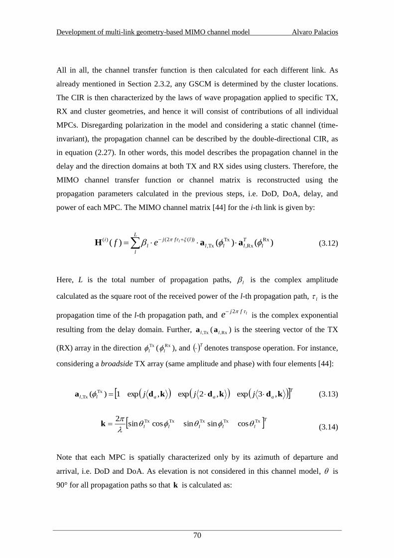
Development of multi-link geometry-based MIMO channel model Alvaro Palacios
70
All in all, the channel transfer function is then calculated for each different link. As
already mentioned in Section 2.3.2, any GSCM is determined by the cluster locations.
The CIR is then characterized by the laws of wave propagation applied to specific TX,
RX and cluster geometries, and hence it will consist of contributions of all individual
MPCs. Disregarding polarization in the model and considering a static channel (time-
invariant), the propagation channel can be described by the double-directional CIR, as
in equation (2.27). In other words, this model describes the propagation channel in the
delay and the direction domains at both TX and RX sides using clusters. Therefore, the
MIMO channel transfer function or channel matrix is reconstructed using the
propagation parameters calculated in the previous steps, i.e. DoD, DoA, delay, and
power of each MPC. The MIMO channel matrix [44] for the i-th link is given by:
L
l
l
T
lll
lfj
l
i lef )()()( Rx
Rx,
Tx
Tx,
))(2()( aaH (3.12)
Here, L is the total number of propagation paths, l is the complex amplitude
calculated as the square root of the received power of the l-th propagation path, l is the
propagation time of the l-th propagation path, and lfje
2 is the complex exponential
resulting from the delay domain. Further, Tx,la ( Rx,la ) is the steering vector of the TX
(RX) array in the direction Tx
l ( Rx
l ), and T denotes transpose operation. For instance,
considering a broadside TX array (same amplitude and phase) with four elements [44]:
Taaall jjj kdkdkda ,3exp,2exp,exp1)( Tx
Tx, (3.13)
Tlllll
TxTxTxTxTx cossinsincossin2
k (3.14)
Note that each MPC is spatially characterized only by its azimuth of departure and
arrival, i.e. DoD and DoA. As elevation is not considered in this channel model, is
90° for all propagation paths so that k is calculated as:

Development of multi-link geometry-based MIMO channel model Alvaro Palacios
71
Tll 0sincos2 RxTx
k (3.15)
For x-oriented arrays, the distance between antenna elements is:
0012
ad (3.16)
For y-oriented arrays, the distance between antenna elements is:
0102
ad (3.17)
Finally, uniformly distributed random phases )(l are applied to the MPCs in order to
create independent channel matrix realizations. This technique that was introduced in
[45] relies on the fact that different realizations of the transfer function can be generated
by changing the phases of the MPCs. This is a well-established fact in radio
communications that theses phases are uniformly distributed random variables, whose
different realizations occur as either TX, RX or clusters move [46]. Therefore, this
technique only requires a single calculation of the propagation parameters of the
channel to get several realizations.
Having calculated all realizations of the channel matrix for each link, the received
power for the i-th link can be expressed as reported in [44], and [47]:
SN
sFi
RTS
i sNNN
P1
2)(
1H (3.18)
where SN , TN , and RN denote the number of channel realizations, TX antennas, and
RX antennas, respectively. Further, )(siH is the s-th realization of the channel matrix
for the i-th link.

Development of multi-link geometry-based MIMO channel model Alvaro Palacios
72
Finally, the MIMO channel matrix for the i-th link and s-th realization is normalized in
the same way as described in [44], and [47]:
i
ii
P
ss
)()(ˆ H
H (3.19)
Hereafter, these channel matrices will be used in the analysis of the inter-link
correlation and consequently in the capacity analysis, as in Section 4.1.
3.3.3 Verification of the channel model
In this section, a simple verification of the multi-link geometry-based MIMO channel
model developed in this work is performed. It must be somehow checked out that the
channel model works properly. To that end, a very simple channel where it is know how
the results should be is used in order to verify that channel matrices, capacities and
correlations are calculated correctly. Figure 22 illustrates the simple dual-link
simulation environment that was chosen for that purpose. In the figure, the simulation
environment contains one common cluster with only one MPC, one MS, two BSs, and
x-oriented arrays in TX and RX with four antenna elements. Link 1 is defined between
MS and BS1 and link 2 between MS and BS2. As the propagation mechanism is only
based on one cluster that is common for BS1 and BS2, the normalized 4 x 4 MIMO
channel matrix for both links should be like:
dddd
cccc
bbbb
aaaa
H (3.20)
where it can be observed that the columns of the channel matrix are equal. This
indicates that the propagation channel seen by the MS side has the same spatial and
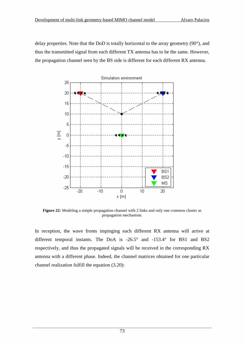
Development of multi-link geometry-based MIMO channel model Alvaro Palacios
73
delay properties. Note that the DoD is totally horizontal to the array geometry (90°), and
thus the transmitted signal from each different TX antenna has to be the same. However,
the propagation channel seen by the BS side is different for each different RX antenna.
Figure 22: Modeling a simple propagation channel with 2 links and only one common cluster as
propagation mechanism.
In reception, the wave fronts impinging each different RX antenna will arrive at
different temporal instants. The DoA is -26.5° and -153.4° for BS1 and BS2
respectively, and thus the propagated signals will be received in the corresponding RX
antenna with a different phase. Indeed, the channel matrices obtained for one particular
channel realization fulfill the equation (3.20):

Development of multi-link geometry-based MIMO channel model Alvaro Palacios
74
Link 1
1965.09805.01965.09805.01965.09805.01965.09805.0
5050.08631.05050.08631.05050.08631.05050.08631.0
7586.06516.07586.06516.07586.06516.07586.06516.0
9294.03691.09294.03691.09294.03691.09294.03691.0
jjjj
jjjj
jjjj
jjjj
Link 2
9959.00907.09959.00907.09959.00907.09959.00907.0
9121.04100.09121.04100.09121.04100.09121.04100.0
7289.06847.07289.06847.07289.06847.07289.06847.0
4662.08847.04662.08847.04662.08847.04662.08847.0
jjjj
jjjj
jjjj
jjjj
As the propagation mechanism is the same for link 1 and link 2, the correlation between
links or inter-link correlation (See Section 4.1 for more details) should be close to one
for all values of significance of common clusters different to 0. Indeed, Figure 23b)
illustrates the expected results for the inter-link correlation. Therefore, the TX
correlation matrices for links 1 and 2 should be the same and all its entries equal to one.
Exactly, the normalized correlation matrices look as expected for both links:
0000.10000.00000.10000.00000.10000.00000.1
0000.00000.10000.10000.00000.10000.00000.1
0000.00000.10000.00000.10000.10000.00000.1
0000.00000.10000.00000.10000.00000.10000.1
jjj
jjj
jjj
jjj
As the inter-link correlation determines the system performance, it might be expected
that the dual-link to single-link capacity ratio (a further explanation can be found in
Section 4.1) will be always close to the theoretical minimum for all significance of
common clusters different to zero. Indeed, Figure 23a) shows the expected results for
the capacity over the significance of common clusters. Figure 23 was obtained under the
assumption that the significance of common clusters is the same for the different links,
as shown in Figure 21a).

Development of multi-link geometry-based MIMO channel model Alvaro Palacios
75
(a)
(b)
Figure 23: Simulation results on a) channel capacity and b) inter-link correlation. As the main
propagation mechanism consist in only one common cluster, the inter-link correlation is always close to
one and, in turn, the dual-link to single-link capacity ratio reaches always the lowest possible value.

Development of multi-link geometry-based MIMO channel model Alvaro Palacios
76
3.3.4 Relation to COST 2100 MIMO channel model
As mentioned in Section 3.2.1, the COST 2100 model is a geometry-based MIMO
channel model capable to simulate multi-link scenarios. However, there are some
relevant differences between the COST 2100 model and the own multi-link geometry-
based MIMO channel model developed in this thesis. Note that COST 2100 model is
the successor of COST 273 model and therefore, there is also an implicit relation with
the COST 273 model in the following comparison. The comparison between the
ongoing COST 2100 model and the channel model developed in this thesis is explained
below:
To begin with, both models follow the same approach since they are a geometry-based
stochastic physical MIMO channel model. They have also a cluster-based structure and
are capable to simulate multi-link scenarios. In both models, clusters are implemented
and treated as a group of MPCs and involves the use two kinds of clusters: common and
uncommon clusters. Both models calculate the power of common clusters as described
in equation (3.3), that is, the significance of common clusters for one specific link. Both
models are double-directional, i.e. they calculate the CIR in delay and direction as in
(2.25) because the generated radio channels are dispersive in the angular and delay
domain. Therefore, the MIMO channel matrices will be derived in both models from the
double-directional channel impulse response.
Although they share this features, the COST 2100 model provides more detailed and
realistic characterization of clusters and MPCs than in the channel model developed in
this thesis (e.g. the COST 2100 cluster-based structure allows to simulate local and far
clusters or reflections by single bounces and multiple bounces). In addition, the COST
2100 model goes further than the own model and includes the concept of VRs in order
to simulate the dynamic behavior of the channel, as explained in Section 3.2.1. It should
be also mentioned that LOS component is not calculated in the own channel model, and

Development of multi-link geometry-based MIMO channel model Alvaro Palacios
77
COST 2100 cluster parameters such as probability of common clusters, lifetime of
common clusters, and disjoint distance of common clusters either.
To sum up, the developed multi-link geometry-based MIMO channel model generates a
static multipath radio channel by single bounce clusters that emulate far scattering and
since there are not VRs, clusters are always active for its corresponding BS. Clusters are
implemented as a conceptual term because they have a simple characterization in
comparison to COST 2100 model. It has been included the option to distinguish
between two types of clusters: common and uncommon, as in the COST 2100 model.
Finally, the MIMO channel calculation is carried out in the same way as in COST
models, i.e. as described in Section 2.5.1.

Development of multi-link geometry-based MIMO channel model Alvaro Palacios
78
4 EFFECT OF COMMON CLUSTERS ON MULTI-LINK
MIMO CAPACITY AND INTER-LINK CORRELATION
The greatest motivation in this thesis is to investigate how the common clusters affect
the ML-MIMO system performance depending on its significance or geometry. As
already mentioned, common clusters for two or more different links are one of the
physical phenomena affecting significantly the correlation between different links in
multi-link scenarios. Hence, radio communication systems depending on the spatial
characteristics of the channel such as MIMO system can be especially deteriorated, e.g.
if multiple links share the same clusters then the inter-link correlation increases and the
spatial filtering of the links becomes difficult. Therefore, it is important to have an
understanding of common clusters because underestimate the significance of common
clusters is not appropriate since it can lead to overestimate the system performance in
system-level simulations.
This chapter is organized in the following way. In Section 4.1, some definitions are
given in order to perform the data analysis that will enable to study the ML-MIMO
channel capacity and the correlation between links. In Section 4.2, previous works
where the dual-link capacity and inter-link correlation are analyzed with measured
channel data from indoor ML-MIMO channels are briefly presented. In Section 4.3, the
capacity and correlation results obtained in this thesis are provided.
4.1 Data analysis
The analysis and processing of the obtained channel matrices are explained in this
section following the same methodology that was conducted in [44] and [47].
4.1.1 Single-link MIMO Capacity
For the single-link case, the vector of received signal can be written as [47]

Development of multi-link geometry-based MIMO channel model Alvaro Palacios
79
nxHy ˆ (4.1)
where H is the normalized channel matrix calculated in (3.19), is the signal to noise
ratio (SNR), and n is a noise vector. Hence, the single-link capacity can be calculated as
[44]:
H
T
NN
CR
HHIH ˆˆdetlogˆ2
(4.2)
where RNI is the identity matrix of size RN , and H
denotes the conjugate transpose.
Finally, considering a dual-link MIMO channel the single-link sum rate capacity would
be 21ˆˆ HH CC .
4.1.2 MIMO Capacity with Interference
For the dual-link case, the received signal can be written as in [48]:
nxHxHy 2211ˆˆ (4.3)
where 1H and 2H represent the normalized channels matrices of the desired and
interfering link. In addition, and are the SNR and the interference to noise ratio
(INR), respectively, and n is a noise vector. Hence, the dual-link capacity with
interference [44], [47] is expressed as
1
211221ˆˆdetlogˆ,ˆ RHHIHH
H
T
NN
CR
(4.4)
where the instantaneous covariance matrix is calculated as

Development of multi-link geometry-based MIMO channel model Alvaro Palacios
80
RN
HIHHR 222
ˆˆ (4.5)
Here, 1H and 2H are the channel matrices of the desired and the interfering user,
respectively. RNI is the identity matrix of size RN and H
denotes the conjugate
transpose. Here, the dual-link sum rate capacity is defined as 1221ˆ,ˆˆ,ˆ HHHH CC .
As far as the results are concerned, the sum rate dual-link channel capacity is compared
with the sum rate single-link channel capacity [47], i.e. the sum-rate channel capacity
with interference cancellation is compared with the sum rate channel capacity with
perfect interference cancellation. Hence, the following relative capacity (RC), i.e. the
dual-link to single-link capacity ratio, measures the percentage of the single-link
capacity and ranges between 0% and 100%:
21
1221
ˆˆ
ˆ,ˆˆ,ˆ
capacityratesumlink-Single
capacityratesumlink-DualRC
HH
HHHH
CC
CC%
(4.6)
4.1.3 Correlation and Matrix Collinearity
Once channel matrices are obtained, a TX correlation matrix is calculated individually
for each link [44]:
S
S
N
sFi
T
N
s
i
H
ii
sN
ss
1
2
1)(
)(1
)()(
H
HH
R (4.7)
where )(siH is an s-th realization of channel matrix for the link i (i = 1, 2), SN the
number of channel realizations, TN the number of transmitter antennas, and H is the

Development of multi-link geometry-based MIMO channel model Alvaro Palacios
81
complex conjugate. Furthermore, the correlation matrix is normalized in order to
remove path losses.
Having calculated the full correlation matrix, the inter-link correlation is investigated as
the collinearity [49] between the correlation matrices )1(R and )2(R . The collinearity
quantifies the channel similarity in the following way:
FF
Htr
)2()1(
)2()1(
)2()1( ,MCRR
RRRR (4.8)
where )1(R and )2(R are the complex-valued matrices to be compared, tr denote the
trace of a matrix, F
denotes the Frobenius norm of a matrix, and H is the matrix
conjugate transpose operation. In general, this measure describes how similar the sub-
spaces of the compared matrices are. The collinearity ranges between zero (no
collinearity, i.e. matrices are orthogonal to each other) and one (full collinearity,
matrices are similar).
4.2 Earlier works
To date, only few contributions have targeted capacity and correlation analysis in multi-
link scenarios. First capacity studies measuring simultaneously multi-user MIMO data
were performed in [50] and [51]. But recently, novel works using measured channel
data have been also performed by Aalto University in the Department of Radio Science
and Engineering in order to analyze the inter-link correlation [44] and dual-link MIMO
channel capacity [47].
In [44] a measurement campaign in a real environment with one TX and two RX was
conducted in order to analyze the inter-link correlation properties between two 4 x 4
MIMO links. In this analysis, after the dual-link channel measurements and data

Development of multi-link geometry-based MIMO channel model Alvaro Palacios
82
processing, the correlation matrices of the links are reconstructed and used to
investigate the inter-link correlation and how the physical propagation mechanisms
produce the inter-link correlation. Conclusions given in this work reveal that the inter-
link correlation arises as a result of the similarity of dominant propagation mechanisms
such as LOS and reflections due to proximity objects, and antenna array geometry.
In [47] the dual-link MIMO channel capacity was analyzed based on simulations and a
channel measurement campaign in an indoor office environment with two 4 x 4 MIMO
links. The measurements were conducted using recently developed measurement system
[52], i.e. using a 5.3 GHz dynamic dual-link dual-polarized wideband MIMO channel
sounder. In order to provide results, the dual-link channel capacity was compared to the
single-link channel capacity. The analysis of the results concluded that the dual-link
channel capacity is more affected by the signal to interference ratio (SIR) than the
spatial separation of the RXs, and the human shadowing produces variations of SIR up
to ±10 dB that cause large fluctuations in the dual-link channel capacity.
4.3 Results
In order to provide results, simulation studies were done using the multi-link geometry-
based MIMO channel model developed in Section 3.3. Each simulation environment is
analyzed based on the previous definitions of Section 4.1. A dual-link case working at
5.3 GHz with NLOS conditions is considered for all conducted simulations.
The results on the dual-link to single capacity ratio and inter-link correlation are
presented for different values of significance ranging between 0 % and 100%. Unless
otherwise noted, the following simulation results consider the same significance of
common clusters for each different link, as shown in Figure 21a).
Initially, a simple simulation environment was created with one common cluster located
between both BSs at [0, 20] and two uncommon clusters around the MS, as seen in

Development of multi-link geometry-based MIMO channel model Alvaro Palacios
83
Figure 24. In the figure, the number of MPCs for each cluster was set to four and the x-
oriented array in TX and RX has four antenna elements. In Table 2 other model
parameters are presented.
Figure 24: First simulation environment studied. MS and BSs are equipped with arrays of 4 antenna
elements. MS-BS1 defines link 1 which contain one uncommon cluster (red circles). Equivalently, MS-
BS2 defines link 2 with its uncommon cluster (blue circles). Finally, black circles denote the common
cluster for link 1 and link 2. As can be observed, the number of MPCs was set to 4 according to [43].

Development of multi-link geometry-based MIMO channel model Alvaro Palacios
84
Table 2: Model parameters for implementation.
Parameter Value
MS position [0, 0] / [m]
BS1 position [-20, 20] / [m]
BS2 position [20, 20] / [m]
Number of uncommon clusters 1
Number of common clusters 1
Number of MPCs 4
Number of channel realizations 100
SNR 15 dB
INR 15 dB
Number of TX antennas 4
Number of RX antennas 4
Array orientation X
Distance between antenna elements 2/
Number of channel realizations 100
SNR 15 dB
INR 15 dB
Figure 25 illustrates the expected results where, in general, the inter-link correlation
increases and the dual-link to single-link capacity ratio decreases with increasing
significance of common clusters. When the significance of common clusters is 0% the
propagation mechanism is only based on the uncommon clusters and the system
performance depends on the cluster geometries. In this case, it can be observed that
different links are not correlated and the dual-link capacity is roughly equal to the
single-link capacity. On the other hand, for 100% of significance of common clusters
the propagation mechanism consists only in the common cluster and then the inter-link
correlation is one whereas the dual-link channel capacity reaches a minimum value
(30% of the single-link channel capacity).

Development of multi-link geometry-based MIMO channel model Alvaro Palacios
85
a)
b)
Figure 25: Results on a) dual-link channel capacity and b) inter-link correlation for the first simulation
environment. It can be observed how a) the dual-link to single-link capacity ratio and b) the inter-link
correlation decreases and increases with increasing significance of common clusters, respectively.

Development of multi-link geometry-based MIMO channel model Alvaro Palacios
86
Secondly, the simulation environment under consideration has the same configuration
(Table 2) than in Figure 24 but different geometry. Here, the uncommon cluster centers
for different links are overlaid in the same location, and so the MPCs could be partially
or totally overlapped. As uncommon clusters behave as common clusters, it is equal to
have a scenario with two common clusters placed in [0, 20] and [10, 0]. Figure 26
shows the simulation environment with this particular geometry.
Figure 26: Second simulation environment studied where the uncommon clusters are overlaid.
Indeed, the main propagation mechanism in this scenario consists in two common
clusters. In Figure 27 it can be seen that the correlation between links is always very
close to one, and so the dual-link capacity decrease. Low values of the dual-link channel
capacity are then observed (20% of the single link capacity) with all significance of
common clusters. Note that the dual-link to single-link capacity ratio remains almost
constant along the significance of common clusters; only small fluctuations are
observed due to the fading of the different propagation paths.

Development of multi-link geometry-based MIMO channel model Alvaro Palacios
87
a)
b)
Figure 27: Results on a) dual-link channel capacity and b) inter-link correlation for the second simulation
environment. As there are only common clusters as propagation mechanism in the channel, the inter-link
correlation was always close to one, and thus the dual-link capacity reached low values compared to the
single-link case for any value of significance.

Development of multi-link geometry-based MIMO channel model Alvaro Palacios
88
Thirdly, the following simulation environment holds the same parameters (See Table 2)
but different geometry of uncommon clusters, as shown in Figure 28. In the figure it can
be seen that the geometry of uncommon clusters is symmetrical respect to the array
orientation.
Figure 28: Third simulation environment studied. Interestingly, here, the uncommon clusters have
symmetric geometry respect to the array. The common cluster still remains in the same position than in
the simulation studies conducted before.
In principle, here, it might be expected the same results than in the first simulation
scenario. Interestingly, Figure 29 shows that the inter-link correlation is always very
high and consequently the dual-link capacity takes low values compared to the single-
link case even if uncommon clusters are not overlaid in the same location. Therefore,
here, the geometry of uncommon clusters and antenna array play an important role in
the ML-MIMO system performance.

Development of multi-link geometry-based MIMO channel model Alvaro Palacios
89
a)
b)
Figure 29: Results on a) dual-link channel capacity and b) inter-link correlation for the third simulated
environment. As consequence of the ambiguity of linear arrays [53], the channel geometry shown in
Figure 28 is especially harmful for the system performance as can be seen here.

Development of multi-link geometry-based MIMO channel model Alvaro Palacios
90
Figure 29 revealed that these results are due to the ambiguity of linear arrays [53] to
distinguish signals impinging on the array from symmetric directions respect its
orientation. For instance, in any linear array using beamforming, if the search is
performed from 0° to 360°, then the mirror image of each signal impinging the array
with respect to 180° is considered as a signal coming from the same direction. In Figure
28 the x-oriented antenna array in the MS is not able to resolve in the spatial domain
those signals travelling through the uncommon clusters. The uncommon cluster for BS1
is seen at angle 135° and its mirror at -135° corresponds to the uncommon cluster for
BS2. These angles cannot be seen as different directions (DoD) due to the ambiguity of
the x-oriented linear array. In such case the simulation environment shown in Figure 28
could be seen as an equivalent scenario with two common cluster locations, as shown in
Figure 30. As a result, the ML-MIMO channel capacity and inter-link correlation are
quite similar to the previous simulation environment (Figure 26) where uncommon
clusters are intentionally overlaid.
Figure 30: Equivalent scenario to the simulation environment shown in Figure 28.

Development of multi-link geometry-based MIMO channel model Alvaro Palacios
91
Even if both directions are parallel to the array, as shown in Figure 31, those directions
cannot be resolved by the array due to the lack of resolution. Interestingly, it was
noticed again a degradation in the ML-MIMO system performance as a consequence of
the clusters and array geometry, as seen in Figure 32.
(a)
(b)
Figure 31: Simulation environments with directions of departure parallel to the MS array.

Development of multi-link geometry-based MIMO channel model Alvaro Palacios
92
a)
b)
c)
d)
Figure 32: a) and c) illustrate the dual-link to single-link capacity ratio and inter-link correlation
respectively for the simulation environment shown in Figure 31a), whereas b) and d) are for the
simulation environment shown in Figure 31b). From these results, it can be concluded that the channel
geometries shown in Figure 31 cannot be resolved for linear array either.
Hence, it can be concluded that the overall system performance might depend on either
common clusters or channel geometry (clusters and arrays). In order to thoroughly
investigate how often each case restrict the ML-MIMO system performance, a set of
1000 samples were taken from simulations that were performed for individual values of
significance of common clusters such as 0%, 1%, 10%, 50%, 99%, 100%. Here, a

Development of multi-link geometry-based MIMO channel model Alvaro Palacios
93
sample can be understood as the obtained value of RC, or MC according to specific
channel geometry after conduct a simulation. For that purpose, it was considered a
random placement of all clusters (common and uncommon). In addition, some model
parameters that were extracted from measurement data in a typical indoor scenario [43]
are used. For instance, it was noticed that the average number of active clusters is 3.69
and the number of MPCs within a cluster is rarely more than five. Table 3 presents the
model parameters configuration that was utilized in order to model an indoor scenario in
a more realistic manner than before.
Table 3: Channel model parameters.
Parameter Value
MS position [0, 0] / [m]
BS1 position [-20, 20] / [m]
BS2 position [20, 20] / [m]
Number of uncommon clusters 3 (random)
Number of common clusters 1 (random)
Number of MPCs 4
Number of channel realizations 100
SNR 15 dB
INR 15 dB
Number of TX antennas 4
Number of RX antennas 4
Array orientation X
Distance between antenna elements 2/
Number of channel realizations 100
SNR 15 dB
INR 15 dB

Development of multi-link geometry-based MIMO channel model Alvaro Palacios
94
Figure 33 shows one possible example of simulation environment. The BSs and MS
were fixed again in the same locations whereas all clusters were uniformly distributed
within simulation environment. The total number of clusters for each link is four and the
number of MPCs within a cluster is also four.
Figure 33: Example of dual-link scenario with 3 uncommon clusters per link and 1 common cluster. The
number of MPCs within a cluster was set to 4. The cluster locations were generated randomly.

Development of multi-link geometry-based MIMO channel model Alvaro Palacios
95
In Figure 34a) it can be observed that for 99% and 100% of significance of common
clusters the ratio between the dual-link and single-link capacity is ranging between 10%
and 25% with 50% of probability. However, for values of significance below 50% the
dual-link to single-link capacity ratio is ranging between 25% and 65% with also 50%
of probability. Moreover, values above 65% are rarely observed for 99% and 100% of
significance; values above 75% are not very common for 50% of significance. In the
extreme cases with low values of significance (below 10%), it can be even reached
theoretical values of 95% but not more. To sum up, lower values of dual-link to single-
link capacity ratio can be reached more probably with increasing significance of
common clusters.
As far as the inter-link correlation is concerned, Figure 34b) shows that curves for 0%,
1% and 10% of significance of common clusters behave similarly. These curves are
almost linear with the inter-link correlation and this situation corresponds to the uniform
distribution of the inter-link correlation between 0 and 1. However, values below 0.6 are
rarely observed for 50% of significance and typically more than 0.95 in the extreme
case, i.e. 99% and 100% of significance of common clusters. In brief, the inter-link
correlation could adopt any value between 0 and 1 with low values of significance of
common clusters, whereas for high significance of common clusters, the inter-link
correlation is always very close to 1 with high probability.

Development of multi-link geometry-based MIMO channel model Alvaro Palacios
96
a)
b)
Figure 34: CDF over 1000 samples of a) dual-link to single-link capacity ratio and b) inter-link
correlation, for each different value of S_common (significance of common clusters)

Development of multi-link geometry-based MIMO channel model Alvaro Palacios
97
Further, it would be also interesting to study a simple scenario where the significance of
common clusters is different for the different links, as shown in Figure 21b). The
following analysis was intended to investigate whether it is meaningful to treat a cluster
as common cluster for the different links when it is very significant only for one of the
links. The analysis is also restricted to a dual-link case with 4 x 4 MIMO links. For
simplicity, one common cluster and two uncommon clusters are again considered, as
seen in Figure 35. The analysis is carried out in four different dual-link scenarios where
the significance of the common cluster for the different links is:
a) %10)1(
common s and %90)2(
common s
b) %90)1(
common s and %10)2(
common s
c) %10)1(
common s and %10)2(
common s
d) %90)1(
common s and %90)2(
common s
First of all, considering the equation (3.4) given in Section 3.2.1, the total significance
of the common cluster for each case is:
a) 3.09.01.0)2(
common
)1(
commoncommon ssS
b) 3.01.09.0common S
c) 1.01.01.0common S
d) 9.09.09.0common S
From these results, it can be concluded that the common cluster in a) and b) as
propagation mechanism should have similar relevance as in c). In order to make sure of
this behavior, an analysis based on simulations is conducted for the different cases.

Development of multi-link geometry-based MIMO channel model Alvaro Palacios
98
Figure 35: Dual-link scenario with one common cluster fixed in (0, 20), and one uncommon cluster per
link whose location is generated randomly.
Figure 35 shows one possible simulation environment with random placement of
uncommon clusters. The rest of model parameters were established as in Table 2.
However, the significance of common clusters was changed for the different links
according to cases a), b), c), and d). Considering this, the CDF was extracted by taking
1000 samples of dual-link to single-link capacity ratio and inter-link correlation. Here, a
single sample is the value taken from the generated environment after simulate.
Figure 36a) illustrates the CDF of the dual-link to single-link capacity ratio.
Interestingly, it can be appreciated that curves corresponding to different significance
for different links have similar evolution than the curve corresponding to 10% of
significance of common clusters for both links. In Figure 36b) the CDF of inter-link
correlation is shown. Therefore, as expected, Figure 36 indicates clearly that cases a)
and b) behave much like c) than d).

Development of multi-link geometry-based MIMO channel model Alvaro Palacios
99
a)
b)
Figure 36: CDF over 1000 samples of a) dual-link to single-link capacity ratio, and b) inter-link
correlation. The simulated curves are shown for the cases mentioned above.

Development of multi-link geometry-based MIMO channel model Alvaro Palacios
100
Intuitively, under the assumption that common clusters have a noticeable difference
between its significance for the different links, e.g. case a) or b), the link with higher
significance will use mainly the common cluster as propagation mechanism. In contrast,
the other link has low significance of common clusters, and thus the main propagation
mechanism consists of its uncommon clusters. Indeed, each link uses different
propagation mechanism as in a dual-link scenario where common clusters have low
significance for both links, e.g. case c), that is, each link using its uncommon clusters.
However, in case d) the common cluster is the main propagation mechanism for link 1
and 2 due to its high significance for both links. As a consequence, the inter-link
correlation is always close to one, as shown in Figure 36b), and values above 65% are
rarely observed for the ratio between the dual-link and single-link capacity, as shown in
Figure 36a).

Development of multi-link geometry-based MIMO channel model Alvaro Palacios
101
5 CONCLUSIONS
As an initial goal of this master‟s thesis, a simple multi-link geometry-based MIMO
channel model was successfully developed. The greatest motivation of this thesis was to
investigate the overall ML-MIMO system performance when two links share the same
clusters. For this reason, it was especially interesting to develop a channel model based
on two kinds of clusters: common and uncommon clusters. Based on earlier studies, it
was observed that common clusters are one of the physical phenomena causing the
correlation between different links. As the developed channel model is then based on
common clusters, it is also capable of controlling the inter-link correlation.
This thesis was started by introducing basic principles and concepts of radio
propagation and MIMO systems. After this, a literature review on MIMO channel
modeling was also given. In this review, physical models and analytical models were
briefly described together with some popular examples from both model types.
The work continued by discussing the motivation on multi-link scenarios as well as a
reviewing briefly earlier works on multi-link scenarios. The channel model developed in
this thesis was presented next, emphasizing in its approach, key features, operating
principles, verification, and relation to other multi-link channel models.
Before starting with the simulation studies, the conducted data analysis was discussed
based on earlier studies related to the issue. Also earlier works investigating the
correlation between links and the dual-link capacity were introduced. After this, the
simulation studies started by analyzing the ML-MIMO channel capacity and inter-link
correlation in different channel representations where the cluster locations were
manually modified to different positions. Results so far showed that, in general,
correlation between links increases whereas dual-link capacity decreases with
increasing significance of common clusters. However, a high correlation between links
and low dual-capacity compared to the single-link capacity was sometimes observed
with all significance of common clusters. In the latter case, it was concluded that

Development of multi-link geometry-based MIMO channel model Alvaro Palacios
102
common clusters are not the main cause limiting the ML-MIMO system performance,
but however, the imposed geometry of clusters and antenna array is what fully
determines the overall system performance. It was found that the reason of this arises
from symmetric or parallel cluster directions to the array which cannot be resolved by
linear arrays due to the lack of resolution.
Next, a set of simulations with random cluster geometries were made in order to
statistically study how often the ML-MIMO system performance might be degraded by
either the common clusters or channel geometry. The reported results revealed that the
inter-link correlation can take any value with low values of significance of common
clusters depending on the channel geometry (clusters and array). As the inter-link
correlation can adopt a wide range of values, the dual-link to single-link channel
capacity can also take any value. However, the inter-link correlation indicated moderate
to very high values whether the significance of common clusters is equal or higher than
50%, respectively.
To conclude the work, it was also considered especially interesting to investigate a dual-
link scenario with one common cluster which has different significance for the different
links and apparently pretty unequal. To that end, a comparison based on simulations
was done in two scenarios with same significance for the different links in order to
investigate which of them had similar behavior. From the observed results, it was found
out that clusters which are common for two links but with large difference between the
significance for each different link cannot be considered as common cluster. As
expected, the ML-MIMO system performance matched more with the scenario where
the cluster that is supposed to be common for the two links has low significance in both
links.

Development of multi-link geometry-based MIMO channel model Alvaro Palacios
103

Development of multi-link geometry-based MIMO channel model Alvaro Palacios
104
References
[1] O. Sallent, J. L. Valenzuela, R. Agustí, Principios de Comunicaciones Móviles,
Edicions UPC, Barcelona, Spain, 2003, 226p.
[2] A. Cardama, L. Jofre, J. M. Rius, J. Romeu, S. Blanch, M. Ferrando, Antenas,
Edicions UPC, Barcelona, Spain, 2002, 468p.
[3] L. Phifer, “802.11n Primer”, Whitepaper, AirMagnet, August 05, 2008,
http://www.airmagnet.com/assets/whitepaper/WP-802.11nPrimer.pdf
[4] Broadcom Corporation, “802.11n: Next-Generation Wireless LAN
Technology”, Whitepaper, April 2006, http://www.buffalo-
technology.com/files/802_11n-WP100-R.pdf
[5] J. Koivunen, “Characterisation of MIMO propagation channel in multi-link
scenarios”, Helsinki University of Technology, Helsinki, Finland, 2007,
http://lib.tkk.fi/Dipl/2007/urn010162.pdf
[6] P. Almers, E. Bonek, A. Burr, N. Czink, M. Debbah, V. Degli-Esposti, H.
Hofstetter, P. Kyösti, D. Laurenson, G. Matz, A. F. Molisch, C. Oestges, and
H. Özcelik, “Survey of channel and radio propagation models for wireless
MIMO systems”, EURASIP Journal on Wireless Communications and
Networking, 2007.
[7] M. Steinbauer, A. F. Molisch, and E. Bonek, “The double-directional radio
channel”, IEEE Antennas and Propagation Magazine, vol. 43, no. 4, pp. 51-63,
2001.

Development of multi-link geometry-based MIMO channel model Alvaro Palacios
105
[8] A. F. Molisch, H. Asplund, R. Heddergott, M. Steinbauer, and T. Zwick, “The
COST 259 directional channel model-part I: overview and methodology”, IEEE
Transactions on Wireless Communications, vol. 5, no. 12, pp. 341-3433, 2006.
[9] H. Özcelik, “Indoor MIMO channel models”, Ph.D. dissertation, Institut für
Nachrichtentechnik und Hochfrequenztechnik, Vienna University of
Technology, Vienna, Austria, 2004, http://www.nt.tuwien.ac.at/mobile
/theses_finished/.
[10] H. Hofstetter, G. Steinbock, “A geometry based stochastic channel model for
MIMO systems”, Forschungszentrum Telekommunikation Wien, Vienna,
Austria, ITG Workshop on Smart Antennas, pp. 194-199, 2004.
[11] http://www.lx.it.pt/cost273.
[12] A. F. Molisch, A. Kuchar, J. Laurila, K. Hugl, E. Bonek, “Efficient
implementation of a geometry-based directional model for mobile radio
channels”, 50th
IEEE Vehicular Technology Conference, vol. 3, pp. 1449-1453,
1999.
[13] J. W. Wallace and M. A. Jensen, “Modeling the indoor MIMO wireless
channel”, IEEE Transactions on Antennas and Propagation, vol. 50, no. 5, pp.
591-599, May 2002.
[14] J. W. Wallace and M. A. Jensen, “Statistical characteristics of measured MIMO
wireless channel data and comparison to conventional models”, in Proceedings
of the 54th
IEEE Vehicular Technology Conference (VTC ’01), vol. 2, pp. 1078-
1082, Sidney, Australia, October 2001.

Development of multi-link geometry-based MIMO channel model Alvaro Palacios
106
[15] T. Zwick, C. Fischer, and W. Wiesbeck, “A stochastic multipath channel model
including path directions for indoor environments”, IEEE Journal on Selected
Areas in Communications, vol. 20, no. 6, pp. 1178-1192, 2002.
[16] A. Saleh and R. Valenzuela, “A statistical model for indoor multipath
propagation”, IEEE Journal on Selected Areas in Communications, vol. 5, no. 2,
pp. 128-137, 2000.
[17] C.-C. Chong, C.-M. Tan, D. Laurenson, S. McLaughlin, M. A. Beach, and A. R.
Nix, “A new statistical wideband spatio-temporal channel model for 5-Ghz band
WLAN systems”, IEEE Journal on Selected Areas in Communications, vol. 21,
no. 2, pp. 139-150, 2003.
[18] Q. H. Spencer, B. D. Jeffs, M. A. Jensen, and A. L. Swindlehurst, “Modeling the
statistical time and angle of arrival characteristic of an indoor multipath
channel”, IEEE Journal on Selected Areas in Communications, vol. 18, no. 3,
pp. 347-360, 2000.
[19] T. Zwick, D. J. Cichon, and W. Wiesbeck, “Microwave propagation modeling in
indoor environments”, in Microwaves and Optronics International Conference,
pp. 629-633, Sindelfingen, Germany, May 1995.
[20] T. Zwick, F. Demmerle, and W. Wiesbeck, “Comparison of channel impulse
response measurements and calculations in indoor environments”, in Antennas
and Propagation Society International Symposium, vol. 2, pp. 1498-1501,
Baltimore, MD, July 1996.
[21] J. P. Kermoal, L. Schumacher, K. I. Pedersen, P. E. Mogensen, and F.
Frederiksen, “A stochastic MIMO radio channel model with experimental
validation”, IEEE Journal on Selected Areas in Communications, vol. 20, no. 6,
pp. 1211-1226, 2002.

Development of multi-link geometry-based MIMO channel model Alvaro Palacios
107
[22] W. Wiechselberger, M. Herdin, H.Özcelik, and E. Bonek, “A stochastic MIMO
channel model with joint correlation of both link ends”, IEEE Transactions on
Wireless Communications, vol. 5, no. 1, pp. 90-99, 2006.
[23] Da-Shan Shiu, G.J. Foschini, M.J. Gans, and J.M. Kahn, “Fading correlation and
its effect on the Capacity of multielement antenna systems”, IEEE Transactions
on Communications, vol. 48, no. 3, pp. 502-513, Mar. 2000.
[24] J.P. Kermoal, L. Schumacher, K.I. Pedersen, P.E. Mogensen, and F.
Frederiksen, “Stochastic MIMO radio chhanel model with experimental
validation”, IEEE Journal on Selected Areas in Communications, vol. 20, no. 6,
pp. 1211-1226, Aug. 2002.
[25] A. M. Syeed, “Deconstructing multiantenna fading channels”, IEEE
Transactions on Signal Processing, vol. 50, no. 10, pp. 2563-2579, 2002.
[26] M. Debbah and R. Müller, “MIMO channel modeling and the principle of
maximum entropy”, IEEE Transactions on Information Theory, vol. 51, no. 5,
pp. 1667-1690, 2005.
[27] A. Burr, “Capacity bounds and estimates for the finite scatterers MIMO wireless
channel”, IEEE Journal on Selected Areas in Communications, vol. 21, no. 5,
pp. 812-818, 2003.
[28] COST 207, “Digital Land Mobile Radio Communications”, Commission of the
European Communities, 1988.
[29] A. F. Molisch, H. Hofstetter, et al., ”The COST273 channel model”, in COST
273 Final Report, L.Correia, Ed., Springer, New York, NY, USA, 2006.

Development of multi-link geometry-based MIMO channel model Alvaro Palacios
108
[30] L. Liu, N. Czink, and C. Oestges, “Implementing the COST 273 MIMO channel
model”, in Proc. NEWCOM-ACoRN Joint Workshop 2009, Barcelona, Spain,
Mar.-Apr. 2009.
[31] N. Czink and C. Oestges, “The COST 273 MIMO channel model: Three kinds
of clusters”, IEEE 10th
Int. Sym., ISSSTA ’08, pp. 282-286, 2008.
[32] http://www.ist-winner.org/.
[33] V. Erceg, L. Schumacher, P. Kyritsi, et al., ”TGn channel models”, Tech. Rep.
IEEE P802.11, Wireless LANs, Garden Grove, California, USA, 2004,
http://www.802wirelessworld.com/8802.
[34] L. Schumacher, “WLAN MIMO channel matlab program”,
http://www.info.fundp.ac.be/~lsc/Research/IEEE_80211_HTSG_CMSC/distribu
tion_terms.html.
[35] M. Steinbauer, “A comprehensive transmission and channel model for
directional radio channel”, in CSOT 259 TD (98) 027, Bern, Switzerland,
February 1998.
[36] V. Erceg, K. V. S. Hari, M. S. Smith, et al., “Channel models for fixed wireless
applications”, Contribution IEEE 802.16.3c-01/29r4, IEEE 802.16 Broadband
Wireless Access Working Group.
[37] C. Oestges, V. Erceg, and A. J. Paulraj, “A physical scattering model for MIMO
macrocellular broadband wireless channels”, IEEE Journal on Selected Areas in
Telecommunications, vol. 21, no. 5, pp. 721-729, 2003.

Development of multi-link geometry-based MIMO channel model Alvaro Palacios
109
[38] 3GPP – 3GPP2 Spatial Channel Model Ad-hoc Group3GPP TR 25.996, “Spatial
Channel Model for Multiple Input Multiple Output (MIMO) Simulations”,
v6.1.0 (2003-09).
[39] International Telecommunications Union, “Guidelines for evaluation of radio
transmission technologies for imt-2000”, Tech. Rep. ITU-R M.1225, The
international Telecommunications Union, Geneva, Switzerland, 1997.
[40] J. Poutanen, K. Haneda, J. Salmi, V.-M. Kolmonen, F. Tufvesson, T. Hult, and
P. Vainikainen, ”Significance of common scatterers in multi-link radio wave
propagation”, TD(10)10069 in 10th
COST 2100 Management Committee
Meeting, Athens, Greece, February 3-5, 2010.
[41] Luis M. Correia (ed.), Mobile Broadband Multimedia Networks – Techniques,
Models and Tools for 4G, Elsevier, Oxford, UK, 2006, 569p.
[42] J. Poutanen, K. Haneda, L. Liu, C. Oestges, F. Tufvesson, and P. Vainikainen,
”Inputs for the COST 2100 multi-link channel model”, TD(10)10067 in 10th
COST 2100 Management Committee Meeting, Athens, Greece, February 3-5,
2010.
[43] J. Poutanen, K. Haneda, L. Liu, C. Oestges, F. Tufvesson, and P. Vainikainen,
”Parameterization of the COST 2100 MIMO channel model in indoor
scenarios”, TD(10)10060 in 10th
COST 2100 Management Committee Meeting,
Athens, Greece, February 3-5, 2010.
[44] V.-M. Kolmonen, K. Haneda, T. Hult, J. Poutanen, F. Tufvesson, and P.
Vainikainen, ”Measurement-based evaluation of inter-link correlation for indoor
multiuser MIMO channels”, IEEE Antennas and Wireless Propagation Letters,
vol. 9, pp. 311-314, April 2010.

Development of multi-link geometry-based MIMO channel model Alvaro Palacios
110
[45] A. F. Molisch, M. Steinbauer, M. Toeltsch, E. Bonek, and R. Thoma, “Capacity
of MIMO systems based on measured wireless channels”, IEEE Journal on
Selected Areas in Telecommunications, vol. 20, no. 3, pp. 561-569, 2002.
[46] W. C. Jakes, Microwave Mobile Communications. Piscataway, NJ: IEEE Press,
1993.
[47] V.-M. Kolmonen, K. Haneda, J. Poutanen, F. Tufvesson, P. Vainikainen, ”Dual-
link capacity analysis of measured time-variant indoor radio channels”,
Electronics Letters, vol. 46, no. 8, pp. 592-593, April 2010.
[48] R. S. Blum, “MIMO capacity with interference”, IEEE Journal on Selected
Areas in Telecommunications, vol. 21, no. 5, pp. 793-801, June 2003.
[49] N. Czink, B. Bandemer, G. Vazquez-Vilar, L. Jalloul, C. Oestges, A. Paulraj,
“Spatial separation of multi-user MIMO channels”, in IEEE 20th
International
Symposium on Personal, Indoor and Mobile Radio Communications, pp. 1059-
1063, Sept. 2009.
[50] J. Koivunen, P. Almers, V.-M. Kolmonen, J. Salmi, A. Richter, F. Tufvesson, P.
Suvikunnas, A. F. Molisch, and P. Vainikainen, ”Dynamic multi-link ndoor
MIMO measurements at 5.3 GHz”, in Proc. European Conf. Antennas
Propagat. (EuCAP ’07), Edinburgh, UK, Nov. 2007, Tu2.9.7
[51] F. Kaltenberger, M. Kountouris, L. Cardoso, R. Knopp, and D. Gesbert,
“Capacity of linear multi-user MIMO precoding schemes with measured channel
data”, in IEEE 9th Workshop on Signal Processing Advances in Wireless
Communications, SPAWC 2008, July 2008, pp. 580-584.
[52] V.-M. Kolmonen, P. Almers, J. Salmi, J. Koivunen, K. Haneda, A. Richter, F.
Tufvesson, A. F. Molisch, and P. Vainikainen, “A dynamic dual-link wideband

Development of multi-link geometry-based MIMO channel model Alvaro Palacios
111
MIMO channel sounder for 5.3 GHz”, accepted for publication in IEEE
Transactions on Instrumentation and Measurement.
[53] C. Proukakis, A. Manikas, “Study of ambiguities of linear arrays”, in IEEE
International Conference on Acoustics, Speech, and Signal Processing, ICASSP-
94, vol. 4, pp. 549-552, Apr. 1994.


113