development of methods to predict high-speed reacting flows in

Development of Methods to Predict High-Speed Reacting Flows inAerospace Propulsion Systems

J. Philip Drummond ∗

NASA Langley Research Center, Hampton, Virginia 23681

This paper discusses the current state-of-the-art of computational capabilities for predicting reacting flowsin high-speed aerospace propulsion systems with an emphasis on the flow fields in scramjets. We begin witha review of the history of efforts to model the scramjet environment and then concentrate on more recentactivities that lead to today’s capabilities. The NASP technology program provided strong motivation foradvancing the computational capabilities of the country in both the government and private sectors. Requiredground test facilities with sufficient test times were limited to around Mach 8, and higher Mach numbers,achievable in pulse facilities, could only be maintained for the order of milliseconds. In addition, the number offacility cycles available to parameterize a given engine flow path were limited, and the facilities were expensiveto operate. Computational capabilities were needed to fill both of these gaps. While the NASP program wasnot successful in developing a vehicle, it did spawn the development of new computational algorithms. TheHyper-X Program beginning in 1995 revived high-speed computational research and development. A flightprogram is the catalyst that drives technology development and synthesizes all of the efforts into a unifiedtool for development of the ultimate experiment, the flight of a hypersonic vehicle. The genesis of most ofthe current day state-of-the-art computational tools for scramjet research and development began with thisprogram. This paper attempts to cover this story from NASP and Hyper-X to the present day.

I. Introduction

Research to develop a high speed airbreathing aerospace propulsion system was underway in the late 1950’s. Amajor part of the effort concentrated on the supersonic combustion ramjet, or scramjet, engine. Work had also begunto develop computational techniques for solving the equations governing the flow through a scramjet engine. Scramjettechnology and the computational methods to assist in its evolution would remain apart another decade, however. Theprinciple barrier was that the computational methods needed for engine evolution lacked the computer technologyneeded for solving the discrete equations resulting from the numerical methods. Even today, computer resourcesremain a major pacing item in overcoming this barrier. Significant advances have been made over the past thirty fiveyears, however, in modeling the supersonic chemically reacting flow in a scramjet combustor. To see how the twofields finally merged, we briefly trace the evolution of the technology in both areas.

Following pioneering efforts of Ferri1 and Digger2 in the 1950’s, a significant increase in the research to developscramjet engine concepts occurred in the 1960’s. In 1965, the NASA Langley Research Center initiated the HypersonicResearch Engine (HRE) Project to develop a high-speed airbreathing technology for application in the propulsion sys-tems of hypersonic cruise vehicles.3 The goal of the HRE Project was to flight test a regeneratively cooled, hydrogenfueled, pylon mounted scramjet on the X-15 research airplane and demonstrate design performance levels. The HREdid not reach the flight demonstration stage due to cancellation of the X-15 program, but the ground-based programdid continue and resulted in the development and construction of two variable geometry engine models. Work withthese models significantly increased the scramjet technology base to be applied in more advanced configurations.

Following completion of the HRE Project, attention moved to propulsion concepts that would provide high per-formance when installed on a vehicle. The original concept, a pylon mounted HRE, would have resulted in excessivelevels of external drag, so the pylon was removed and work began to highly integrate the engine with the airframeof candidate vehicles. In addition, engine weight was reduced by moving from a variable to a fixed geometry whichreduced the engine structure. Out of this activity, the Langley airframe integrated scramjet engine concept was con-ceived. This program has continued to the present day, and has resulted in the successful demonstration of the conceptto produce net thrust in subscale hardware. A detailed review of this program was given by Northam et al.3

In addition to the NASA scramjet research and development program, other government activities included a Navysponsored scramjet program at the Applied Physics Laboratory of the Johns Hopkins University (JHU/APL) 4,5. Thiswork also increased in the 1960’s and was directed towards the development of an air-breathing shipboard missileusing a scramjet propulsion system. Development of this concept continued until 1977. At that time, concern overthe storage of the highly reactive and toxic fuels to be used forced a change to more conventional but safer fuels.

∗Distinguished Research Associate, AIAA Associate Fellow; email: [email protected]

1 of 29

American Institute of Aeronautics and Astronautics

This change resulted in the development of an integral-rocket/dual-combustor ramjet concept that used a fuel-rich gasgenerator to preburn the fuel for a main supersonic combustor, thus allowing the use of hydrocarbon fuels.6

The Air Force also sponsored scramjet research and development during the 1960’s.4 They continued the supportof several programs that were initially funded by the HRE program. In 1964, a program was started at the GeneralApplied Science Laboratory to continue development of a low-speed fixed-geometry scramjet engine. A dual-modescramjet program was continued with the Marquardt Company at the same time. Soon thereafter in 1965, the AirForce began an effort with the United Aircraft Research Laboratory to continue development of a water cooled variablegeometry scramjet design. These three efforts ended in 1968, and only the NASA and JHU/APL programs continuedinto the 1970’s.

During the 1970’s, computational techniques were first applied to study the supersonic reacting flow found in ascramjet combustor. A detailed review of those activities is given by White, et al.4 A summary of that discussion andadditional work is now provided. Some of the earliest work to model supersonic reacting flows was by Ferri7 and hiscolleagues, Morretti8, Edelman9, and Dash.10,11 They employed an explicit viscous characteristics method that splitthe governing equations into hyperbolic and parabolic parts, followed by a coupled numerical solution of each part ateach integration step. Modeling multistep finite-rate chemistry was also included in their solution strategy. Spaldingand his colleagues then took Ferri’s splitting-based approach and improved its efficiency by developing a fully implicitsolution procedure for solving the governing equations.12 Spalding then developed several implicit parabolized Navier-Stokes programs for modeling scramjet combustor flow fields. These codes included the CHARNAL two-dimensionalaxisymmetric program13 and the SHIP three-dimensional program.14 Both programs used the well known SIMPLEsolution procedure for spatially marching the governing equations in the parabolized direction while employing atridiagonal matrix solution procedure to perform repetitive sweeps for solution of the equations in the cross-plane(s).15

These programs assumed that a state of chemical equilibrium always existed, but they were later modified by Evans16

to include the effects of finite-rate chemical reactions. The modified programs were still being used in the mid-2000sfor studies of mixing and reaction in combustor configurations.

The work of Ferri and Spalding was then adapted by Dash to develop the SCORCH program that used a hybridexplicit-implicit procedure for modeling supersonic reacting flows. The method again split the governing equationsinto hyperbolic and parabolic parts. The hyperbolic part was solved using a viscous characteristics approach thatemployed an upwind finite-difference procedure. The parabolic part was solved using an implicit finite-differenceprocedure.17 Work on this program and its application to supersonic combustion problems has continued to the presentday.

While Ferri, his colleagues, and Spalding were developing analysis techniques for direct application to the super-sonic reacting flow problem in a scramjet, other algorithm developments were underway, directed primarily at solvinghigh-speed external flow problems. These techniques ultimately found their way, however, into the internal reactingflow arena. The first of these algorithms was the MacCormack explicit, unsplit predictor corrector method initiallydeveloped to model the hypervelocity impact cratering problem.18 The MacCormack method was a variation of theLax-Wendroff second-order accurate scheme that could be applied to complex geometries. Because of these qualities,the algorithm was readily adopted and used to study a wide class of external flow problems. Implicit algorithms werealso developed for external flow problems in the 1970’s, motivated by the need to resolve the high gradients presentin wall boundary layers. The resolution of boundary layers requires fine computational grids, resulting in a severestability constraint on the marching time step size of an explicit method. Where only a steady state solution was re-quired and time accuracy was not necessary, implicit methods converged much more rapidly. Early work to developimplicit solution techniques for the Navier-Stokes equations was carried out by Briley and McDonald19 and Beam andWarming.20 Both approaches used a spatial factoring procedure that reduced the multidimensional problem to one ofsequentially solving a set of one-dimensional spatial implicit operators. Using this computationally efficient proce-dure, convergence rates one to two orders of magnitude faster than the explicit method were achieved for steady-stateproblems on highly stretched grids.

While the application of implicit methods was generally limited to scramjet inlet flow fields through the late1970’s and early 1980’s, explicit methods were applied extensively in studies of combustor flow fields. In 1977,Drummond developed the two-dimensional TWODLE combustion program, based on the MacCormack method, tomodel internal scramjet combustor flow fields. The code used an equilibrium chemistry scheme to model H2-airreaction and several algebraic eddy viscosity methods to model the turbulence field. The program was applied toseveral scramjet combustor component problems. Particular emphasis was given to the scramjet fuel injector problemin an attempt to better understand the complex flow field in this region of the engine.21,22 Development on the programcontinued into the early 1980’s when the program was used to carry out the first simulation of a scramjet flow fieldusing a two-dimensional model engine module.23 Detailed studies to optimize the configuration of the scramjet fuelinjectors were also completed during this period.24,25

An explicit solution procedure was also employed by Schetz during the early 1980’s to model the APL dual-combustion ramjet described earlier.26 He employed a modular approach to carry out his analysis. The mixing andburning of the center jet from the fuel-rich gas generator was calculated with a jet mixing code27,28 that was modifiedto include a turbulent kinetic energy mixing model, a chemistry model, and other improvements. Because of the high

2 of 29


static pressures and temperatures that were present in the device, a local diffusion-controlled, equilibrium chemistrymodel was used to model reaction in the combustor. Schetz’s procedure for modeling combustor flows was ultimatelycombined with an inlet analysis procedure to compute performance estimates for the dual-combustion ramjet.29

While numerical methods for modeling scramjet flow fields were developing through the 1960’s, 1970’s and early1980’s, there was a parallel growth in computer hardware upon which these methods could be applied. Many of theearly calculations were carried out on IBM 7090 and CDC 6600 class machines. Hardware improvements, that allowedthe consideration of more realistic problems, came in the late 1960’s with the arrival of the CDC 7600 computer. Themost significant hardware improvement came in the mid to late 1970’s, however, when vector processing supercom-puters became available to the computational community. These machines included the CDC Star-100 and the Cray1, followed in the early 1980’s by the Cyber 205 and the Cray X-MP which gave performance capabilities severalorders of magnitude greater than the previous scalar machines.4 Until this time, the state of computer resources hadresulted in a major barrier to advancing the state of the art in modeling supersonic reacting flows. With the Cyber 205and Cray X-MP, however, the researcher was now in a position to begin dealing with the detailed physics containedin these complex flows. The burden now returned at least partially to the state of numerical algorithms used to modelsupersonic combustion. Later experience would show that an even greater challenge rested in the physical modelingused to describe the flow physics in high-speed propulsion systems.

II. NASP and Early Code Development Efforts

As previously described, only the NASA and JHU/APL hypersonic programs continued into the 1970’s.30 Bothprograms were limited to ground based experimental programs and modest theoretical and computational programsto guide and analyze the experimental efforts. A new national hypersonics program was needed to spur developmentand the need for more advanced theoretical and computational tools. The program to develop a single-stage to orbithypersonic vehicle, the National AeroSpace Plane, or X-30, shown in Figure 1 began as a joint Air Force NASAprogram in 1985. That program had actually been underway since 1982 as a highly classified Defense AdvancedResearch Projects Agency (DARPA) project called Copper Canyon.31 Ronald Reagan, in his 1986 State of the UnionAddress, described the program as “a new Orient Express that could, by the end of the next decade, take off fromDulles Airport and accelerate up to twenty-five times the speed of sound, attaining low earth orbit or flying to Tokyowithin two hours.” Unfortunately, the goals of the Orient Express and other uses of a single-stage to orbit vehicle werenot achieved during the program. The related technology program for both an orbital and hypersonic cruise vehiclelasted for over 13 years, however, and other programs, albeit more modest or realistic, have continued to the presentday.

The NASP technology program provided strong motivation for advancing the computational capabilities of thecountry in both the government and private sectors. Ground test facilities with sufficient test times were limited toaround Mach 8, and higher Mach numbers, achievable in pulse facilities, could only be maintained for the order ofmilliseconds. In addition, the number of cycles available to parameterize a given engine flow path were limited, andthe facilities were expensive to operate. Computational capabilities were needed to fill in the gaps. Short term effortsconcentrated on extending existing capabilities for the simulation of high-subsonic and supersonic, turbulent reactingflows.

One of the first efforts in this new hypersonic program involved extension of the TWODLE code32 initially devel-oped as a high-speed combustion research tool to include detailed models for finite-rate chemistry and kinetic-theory-based models for the molecular diffusion of momentum, heat, and species. This extended code evolved into the SPARKcombustion program utilized in a number of early studies of the Copper Canyon and NASP flow paths. Carpenter33

extended the SPARK code to three dimensions and added generalized equilibrium chemistry and finite-rate chemistrymodels that allowed consideration of any fuel-air system with any number of reaction paths.34 Three-dimensionalparabolized Navier-Stokes programs were also developed to model supersonic combustor flow fields. These programsprovided a more efficient solution procedure if the flow field contained no subsonic regions. Chitsomboon developeda three-dimensional parabolized Navier-Stokes (PNS) program35 by extending a two dimensional PNS program thathe had developed earlier.36,37 He solved the conventional parabolized Navier-Stokes equations together with a set ofspecies continuity equations. A new three-dimensional explicit upwind PNS algorithm based on Roe’s flux-differencesplitting was then developed by Korte.38 The method was second order accurate in the marching direction as wellas the cross-stream directions. The algorithm was extended by White to include finite rate chemical reactions. Inaddition, the unsteady Riemann problem, rather than the steady Riemann problem used in the original formulation,was solved using the unsteady Riemann solver of Roe.39 During this same period, Gielda developed a non-reactingthree-dimensional explicit PNS program40 using the MacCormack explicit algorithm.18 Gielda extended his code tomultiple species by adding the parabolized species continuity equations to the governing equation system.41 He alsoincorporated both an equilibrium and a global one-step H2-air finite rate scheme into the program. Kamath then em-ployed the Gielda algorithm to develop a parabolized version of the three-dimensional SPARK combustion code.33 Hegeneralized the coordinate transformation to allow the streamwise coordinate to be orientated in the most supersonicdirection. He also used the generalized equilibrium and finite rate chemistry schemes developed by Carpenter34 so any

3 of 29


Figure 1: Artist’s concept of NASP X-30 hypersonic vehicle

multistep reaction scheme could be considered with the algorithm. All of these codes were vectorized to run efficientlyon available vector supercomputers of the day including the Cray 2 and the Cyber 205.

In addition to the codes extended or sponsored by NASA, the codes developed by Spalding, Dash, MacCormack,and their colleagues continued to be popular tools for modeling supersonic reacting flows typical of those foundin scramjet combustors. The Spalding three-dimensional parabolized Navier-Stokes code, SHIP14, as modified byEvans,16 was still being used to carry out engineering design studies of scramjet configurations as well as basichigh speed fuel-air mixing studies. The two-dimensional parabolized Navier-Stokes code, SCORCH, of Dash17 sawconsiderable use performing analyses of the NASP propulsion system. In addition, the code was also used to carry outseveral fundamental studies of experiments being used to design that propulsion system.

The development of a number of new algorithms was underway in the early or mid-1980s with the majority fallinginto the general class of monotone methods, that is, methods that employed flux-correcting or flux-limiting proceduresto preserve high numerical resolution without the numerical oscillations associated with higher accuracy. Included inthis class of algorithms were Flux Corrected Transport (FCT) methods, total variation diminishing (TVD) methods,and TVD-like methods that exhibit TVD behavior. These algorithms offered the modeler advantages over the previousmethods when studying scramjet problems. Many of the codes utilizing these algorithms were developed to modelsupersonic or hypersonic flow with interacting air chemistry moving about configurations of interest.

The first monotone method applied to chemically reacting flows was the Flux Corrected Transport (FCT) algorithmdeveloped by Boris and Book42–44. Its development actually began in the 1970s and was revisited for propulsive flowsin the late 1980s. In this method, a small amount of artificial diffusion was added to the governing equations in smoothregions of the flow to stabilize the solution. In regions where high gradients existed, larger amounts of diffusion wereadded to maintain monotonicity. The diffusion was added in such a manner that the overall dissipation was held belowthat of the earlier algorithms because most of the diffusion was subsequently removed. Zalesak later generalizedthe approach allowing the method to be readily incorporated into existing algorithms that did not provide monotone

4 of 29


behavior.45 In addition, the method could be more easily generalized to two and three spatial dimensions. A morerecent discussion of the method was given by Oran.46

Much of the new work was motivated by the need to model external flows about hypersonic vehicles includingNASP as well as reentry vehicles. Therefore, the methods were developed to model high-speed strongly shocked flowsundergoing air chemistry. To compute flows of this type, MacCormack and Candler developed an implicit flux splitscheme, as an extension to MacCormack’s explicit predictor-corrector finite difference method,18 to solve the Navier-Stokes equations. MacCormack initially developed the implicit algorithm to consider only nonreacting flows.47 Afinite volume approach was used to discretize the flux terms. In addition, Steger-Warming48 flux vector splittingwas introduced to more properly account for the propagation of information through the flow field. A finite volumeapproach was used to discretize the flux terms. In addition, Steger-Warming48 flux vector splitting was introduced tomore properly account for the propagation of information through the flow field. Following development of the basicalgorithm, Candler and MacCormack extended the method to consider high-speed air flows that were ionized andin thermodynamic and chemical nonequilibrium.49,50 Subsequent successes modeling flows with air chemistry madeit apparent that the algorithms could readily be modified to consider internal flows with combustion chemistry, and,therefore, serve as a means for modeling scramjet combustor flow fields.

Flux splitting methods were also employed by Grossman, Walters, and Cinnella to model high speed chemicallyreacting flow problems. Grossman and Walters initially developed their algorithm to solve the Euler equations fornonreacting flows, but included real gas effects.51 Three forms of flux splitting were considered,including Steger-Warming flux vector splitting,48 van Leer flux vector splitting,52 and Roe flux difference splitting.53. Each of thesesplitting methods was originally derived to be applied to ideal gas flows. They were rederived by Grossman51 to allowtheir application to problems with real gas effects. The flux split equations were solved using a two-step predictor-corrector method that was second-order accurate in space and time. Spatial differences were formed using the MUSCLdifferencing procedure and flux limiting by Anderson.54 Following the successful application of the algorithm to aone-dimensional shock tube problem, real gas splitting was incorporated into a two-dimensional implicit finite volumecode that originally utilized van Leer splitting and Gauss-Seidel line relaxation to solve the equations governing idealgas flows.55

Grossman and Cinnella then extended the algorithms to include vibrational and chemical nonequilibrium56,57

by appending species continuity equations to account for each chemical species present in the reacting flow andvibrational energy conservation equations to account for those species in vibrational nonequilibrium. The authors thenredeveloped the relationships described previously that were required to implement Steger-Warming, van Leer, andRoe flux splitting. Once these splitting approaches had been implemented, a finite volume scheme was used along witheither an explicit Runge-Kutta time integration or an implicit Euler time integration to solve the governing equations.Nonequilibrium effects were modeled with a five species, five-reaction model that included N2, O2, NO,N, and O.Extensions of the algorithm to two- and three-dimensions were then carried out.

Additional interesting work using flux splitting was also conducted by Liou, van Leer, and Shuen.58 The authorsagain employed van Leer flux vector splitting or Roe flux difference splitting and derived real gas versions of theseapproaches. The derivations were begun by assuming a general equation of state for a real gas in equilibrium. Ap-proaches similar to those discussed previously were then used to modify the splitting, but the number of assumptionsemployed were kept to a minimum. The modified splitting was then incorporated into an available TVD algorithm59

and used to model several problems described by the one-dimensional Euler equations. The algorithm was then ex-tended to two- and three-dimensions.

A considerable amount of work was also undertaken to develop new TVD schemes for chemically reacting real gasflows. Beginning in 1985, Yee developed a symmetric TVD scheme that could be employed in the context of eitherexplicit or implicit numerical integration procedures.60 The approach was later generalized to consider chemicallyreacting flows.61 Yee noted that her approach could readily be added to existing algorithms that did not exhibit TVDbehavior, e.g. the 1969 MacCormack method, resulting in a more robust method with better shock capturing qualities.New explicit, semi-implicit, and implicit algorithms employing the symmetric TVD method were then developed anddiscussed.61 An explicit multistep TVD scheme was constructed using the 1969 MacCormack method18 for the firsttwo (predictor-corrector) steps followed by the addition of a conservative dissipation term as a third step, such that theoverall scheme was TVD. The dissipative term was made up of products of eigenvectors of Jacobians of the governingequation system and their associated eigenvalues, an entropy correction, and a limiter function. Details regarding theconstruction of the dissipative term and the determination of its magnitude is given in the reference.62 Finally, a fullyimplicit TVD method was developed including both implicit source and flux terms for situations where both chemistryand fluid scales were small and of the same order.61

When implicit alternating-direction implicit (ADI) procedures were used, the factorization error that resulted whenthe implicit operator was spatially factored could not be neglected in some calculations. An alternate proceduredeveloped by Gnoffo employed point implicit relaxation.63,64 Gnoffo used this procedure in his three-dimensionalfinite volume code with a symmetric TVD upwind discretization of the governing Navier-Stokes, species continuity,vibrational, and electron energy equations. Pseudo-time relaxation was used to drive the solution to a steady state. Thisprocedure proved to be very efficient on vector computers. Two options for coupling the governing fluid and chemistry

5 of 29


equations, strong and weak implicit coupling, were also utilized. With strong implicit coupling, the complete equationset was solved as a unit, an approach typical of those described earlier. Weak implicit coupling involved splittingthe fluid and chemistry equations into two groups, and applying the point-implicit method to each group separatelyduring the relaxation process. The former approach was more physically exact, better accounting for complex waveinteractions and fluid-kinetic coupling. The latter approach allowed for the relaxation strategy and time stepping tobe tailored to the needs of the equation set 64. Air chemistry was modeled in the program using an eleven speciesscheme that included N,O,N2, O2, NO,N

+, O+, N+2 , O

+2 , NO

+, and e−. Further details on the chemistry modeland other physical modeling are given in the reference.65

Another attractive alternative to an ADI integration scheme for solving the spatially discretized governing equa-tions was a lower-upper (LU) scheme that approximately splits the implicit operator into upper and lower operatorsthat are independent of the dimensionality of the problem. Shuen and Yoon developed a scheme for solving the two-dimensional Navier-Stokes and species continuity equations governing chemically reacting flows that employed animplicit finite-volume time marching LU method.66 Details of the derivation of the LU scheme are given in by Shuen,et al.66 The approach was attractive because, even though the method was fully implicit, it required only scalar diag-onal inversion for solution of the flow equations and diagonal block inversion of the species equations. The authorsstated that as a result, the scheme exhibited a fast convergence rate while requiring only about the same amount ofwork as an explicit method.66 This advantage was particularly important when problems with a large number of chem-ical species were being solved. Following development of the LU code RPLUS using this technique, an eight species,fourteen-reaction chemistry model and an algebraic turbulence model were added to the program. Encouraged by theirsuccess, Yu and Shuen then extended the LU code to three-dimensions (RPLUS3D).67

With the exception of Flux Corrected Transport, the methods described in the previous paragraphs have exhib-ited second-order numerical accuracy in both space and time. Two high-order accurate methods were also developedand applied to high-speed combustion problems. These methods offer improved accuracy and reduced phase error.One method was developed by Carpenter using a fourth-order compact finite-difference scheme.33 The scheme wasinitially developed by Abarbanel to accurately solve the Euler equations in two- and three-dimensions.68 Carpenterextended these ideas to the Navier-Stokes equations and used them to alter the 1969 MacCormack method, producinga fourth-order “compact MacCormack” scheme. The modifications did not change the basic structure of the MacCor-mack scheme, allowing it to be easily incorporated into existing codes using the 1969 algorithm. The modificationsignificantly improved the accuracy of the algorithm, while markedly reducing the phase error. As a result, the im-proved scheme was able to crisply capture strong shocks with very little of the pre- and post-shock oscillations presentin the old scheme. The algorithm in fact exhibited a TVD like behavior when capturing waves.

High-order accurate spectral methods were also applied to supersonic reacting flows. Drummond extended aChebyshev spectral method developed for studying transitioning flows69,70 to include finite rate chemical reactions.71

To apply this method to the Navier-Stokes and species continuity equations, the flux terms in these equations wereexpanded in terms of Chebyshev series, and then the required spatial derivatives were taken. The resulting ordinarydifferential equations were then integrated with respect to time using a Runge-Kutta time stepping scheme. Drummondinitially developed this technique for the one-dimensional Euler equations and species continuity equations.71. Themethod was then extended to multiple dimensions where a hybrid spectral-finite difference algorithm was used tomodel two-dimensional supersonic reacting flows.72

Many of these high-speed code development activities reached some degree of maturity toward the end of theNASP era, but much work remained. In the late 1980s and early 1990s, the NASP program began to contract, althoughit was sustained for several years by a technology development program. This program allowed some of the morefundamental activities that we have discussed to continue, including computational and flow diagnostic development,and flow path research. Absent however was the all important flight program that either needed to be underway or atleast planned for the near future. A flight program is the catalyst that drives technology development and synthesizesall of the efforts into a unified tool for development of the ultimate experiment, the flight of a hypersonic vehicle.Hypersonics research has gone through several cycles in the United States over the past 60 years. Fortunately theNASP program was followed in the next few years by another “cycle,” the Hyper-X flight program. The “run-up” toHyper-X sustained the fundamental computational, diagnostic and experimental programs allowing them to mature tothe supporting role that was required for a successful flight program.

III. Hyper-X and a New Generation of High-Speed Reacting Flow Codes for Scramjets

Following more than 40 years of ground-based scramjet research and testing, a strong consensus developed in thehypersonic propulsion community for moving air-breathing technology from ground facilities to flight. Even thoughmuch had been achieved in ground-based facilities, it was impossible to duplicate the complexities of hypersonic flightwithout flying in the atmosphere. From this recognition, the Hyper-X Project evolved in late 1995 as a joint effort of theNASA Langley and Dryden Research Centers.73,74 The program was planned to utilize a 12 foot hypersonic vehiclewith a scramjet propulsion system to be launched from a B-52 aircraft and accelerated to hypersonic speeds by aPegasus rocket. The stack (the Hyper-X aircraft and the rocket) was carried under the wing of the B-52 as shown in

6 of 29


Figure 2.A layout of the Hyper-X vehicle is given in Figure 3. The vehicle was 148 in. long and 60 in. wide at the maximum

extent between the tail fins. The scramjet propulsion system was 30 in. long and 19 in. wide. For flight, the vehiclewas flown to around 40 thousand feet and then dropped from the carriage beneath the wing of the B-52. The Pegasusrocket was then ignited to boost the vehicle to around 95 thousand feet. At that altitude, the rocket and vehicle wereseparated, and the scramjet engine was ignited allowing the vehicle to cruise under its own power. Two successfulHyper-X flight tests at Mach 7 and Mach 10 were flown in March and November of 2004.

Figure 2: Hyper-X launch stack beneath wing of B-52

Figure 3: Hyper-X layout and overall dimensions (in).

The Hyper-X Program brought a resurgence of effort in hypersonics including wind tunnel and flow path test-ing and more fundamental work in measurement diagnostics, chemical kinetics and non-reacting and reacting flowsimulation and modeling. We will concentrate in this paper on the code development and modeling activities.

7 of 29


A. Evolution of RANS and LES/RANS Combustion Codes

Much of the early work associated with the Hyper-X Program was fundamental in nature. As a consequence, thedevelopment of new combustion codes tended to focus on capabilities for detailed analyses of the engine flow field.Computer resources were still limited, but by constraining analyses to critical regions of the scramjet, reasonableanalyses were possible. Codes were developed to study the fuel injection process and the mixing and combustion offuel and air downstream of injectors. Detailed fuel injector design was also considered in order to enhance fuel-airmixing and enable the highest level of mixing and combustion efficiency.

Hyper-X was a flight program, however, and understanding critical regions of the engine flow field was extremelyimportant, but only part of the problem facing researchers. The overall engine flow path had to be designed, andthat design depended on both experimental research and computational analyses. Ground based facilities, where theexperimental work was conducted, functioned in the lower Mach number range of the vehicle and were expensiveto operate. Computational tools were needed to establish initial designs for testing and to fill in the regions betweentest points in the facilities. As a consequence, code development forked in two directions with one branch continuingalong theoretical grounds and the other concentrating on the development of design codes. The development of thesecodes over a number of years produced many of the programs in use today for both fundamental studies and designcodes. Some of the codes in fact served both purposes. We will trace the development of these codes for the remainderof this paper. Program development that was initiated to create codes for commercial use will not be considered in thispaper. In addition, not every code capable of simulating high-speed reacting flows will be discussed, but the authorwill attempt to cover every class of code that is capable of performing these analyses.

One of the first efforts to develop a code for scramjet development began in 1987. The GASP code solved thesteady and unsteady Euler, parabolized Navier-Stokes, thin-layer Navier-Stokes, and Navier-Stokes equations. Itutilized as options preconditioning, approximate factorization, line Gauss Seidel, Generalized Minimal Residual,75

mesh sequencing and multi-grid. Inviscid flux definition in GASP utilized several options, including Roe’s and VanLeer’s upwind biased formulations and central differencing with artificial viscosity. Central differences were used todefine viscous fluxes. Both algebraic and two-equation turbulence models with wall function options were used inthe code. Generalized zonal-boundary interpolation was used across zonal intersections defined by a single logicalboundary. Parallel processing was employed on shared memory computer architectures. A set of thermochemicalkinetic models was provided for air chemistry, hydrogen-air combustion, and various hydrocarbon reactions in adatabase containing 455 reactions and 34 species. Thermal nonequilibrium was modeled using a separate vibrationaltemperature for each molecule or a lumped vibrational temperature common to all molecules.76 GASP was validatedfor a number of external and internal flow fields.77–79 The code was then employed to analyze the external flow fieldsabout a number of hypersonic vehicles and high-speed engine flow paths.

Another initial effort to develop a new code for scramjet flow path design was undertaken at the NASA LangleyResearch Center. The LARCK code development project began in the early 1990s as a replacement for the SPARKcombustion code. The program that evolved was a cell-centered, finite volume, multi-block, multi-grid, code tosolve the full Reynolds averaged Navier-Stokes (RANS) equations for turbulent non-equilibrium chemically reactingflows.80,81 The code contained a generalized thermodynamics model for an arbitrary mixture of thermally perfect gasesand an Arrhenius based finite-rate chemistry model with a generalized scheme that allowed for the specification of anychosen reaction model. Turbulence models included the Spalart-Allmaras model,82 the Wilcox high and low Reynoldsnumber k−ω models, Wilcox’s compressible pressure gradient corrected wall matching procedure,83 Menters baselineand SST models,84,85 the k− ε low Reynolds number model of Abid et al.,86 and the algebraic Reynolds stress modelsof Abid87 and Adumitroaie.88 Coupling between the turbulence and chemistry fields was also accounted for withGaussian or beta assumed probability density functions to account for temperature variance effects on forward andbackward kinetic rate coefficients in the chemistry model.89 Turbulence effects on the species production rates werealso accounted for by modeling the sum of the species variances using a multivariate assumed probability densityfunction.90 The LARCK code was validated against a number of 2-D and 3-D unit problems such as the flat plateflow91, high Mach number compression ramp flow, and Mach 3 corner flow. It was then used to model individualscramjet component flows as well as the entire flow path in a scramjet engine.

The LARCK code served as a predecessor for another new analysis code for high-speed flows that has becomea standard for simulating external and internal flows even to the present day. A program to develop the VULCANcode began in 1996 as a part of a ramjet-scramjet CFD code development effort at the Wright Patterson Air ForceBase. The foundation program was developed at that time under an Air Force contract. The next year, the programdevelopment effort moved to the NASA Langley Research Center, and work has continued at the Center until thepresent day. Like its predecessor the program solved the equations governing two- and three-dimensional caloricallyperfect or thermally perfect non-equilibrium chemically reacting flows. The code used a structured grid, cell centered,finite volume, density based method.92,93 Inviscid fluxes were computed to second order accuracy using van Leer’sMUSCL scheme with either the flux difference split scheme of Roe or the low dissipation flux split scheme of Edwards.Viscous fluxes were computed to second order accuracy using either a thin layer gradient or full gradient construction.The full spatially elliptic Euler or full Navier-Stokes equations were solved by integrating the conservative form

8 of 29


of the unsteady equations in real or pseudo-time (where only a steady-state solution is desired). Time-derivativepreconditioning allowed the code to be applied to low speed flows even though it had been primarily developed forhigh-speed regimes.94 In addition, the code could solve the spatially hyperbolic Euler or parabolized Navier-Stokesequations. By using a four level hierarchy of domain decomposition, grouping finite volume cells into blocks andblocks into regions, an entire physical domain could be discretized into a computational domain (the fourth level) foranalysis.

Chemical reaction was modeled in the VULCAN code using a generalized Arrhenius based model.93 Any numberof reactions in an overall reaction mechanism could be considered. Global reaction models were often consideredwhere possible to reduce the number of chemical reactions and species being solved. Mean flow turbulence modelsused in the code included the k− ε and k−ω models previously used in the LARCK code as well improved turbulentkinetic energy models that were being developed in parallel with VULCAN. Interactions between the turbulence fieldand chemistry were modeled with an assumed beta probability density function (PDF) to account for the effects oftemperature fluctuations on chemical reaction rates and a multivariate assumed beta PDF to account for the effectof species fluctuations on species production.89,90 However, the statistical dependence among the scalars was notaccounted for by these models.

Figure 4: Schematic of staggered ramp injector configu-ration

Figure 5: Schematic of staggered strut injector configu-ration

Figure 6: Computational grid for the ramp injector con-figuration

Figure 7: Computational grid for the strut injector con-figuration

One of the first uses of the VULCAN code was the investigation of advanced fuel injection schemes for scramjetengines. The code was used to evaluate the cold flow mixing effectiveness of two fuel injection schemes, a rampinjector and a strut injector, being considered for new scramjet designs.92 The two injector designs are shown inFigures 4 and 5. Helium was used as the fuel simulent. Cold flow simulations were conducted for each design. Thegrid system for each configuration is shown in Figures 6 and 7. Mass fraction contours from the simulations for bothconfigurations are shown in Figures 8 and 9. The authors note “the effect of streamwise vorticity generated along thesides of the ramps is clearly evident in the fuel plume at the 4-inch cross stream plane. A relatively strong obliqueshock is formed in the next 4-inch segment of the combustor through the interaction of the incident ramp shocks andthe underexpanded jets. This shock wave turns the fuel plume towards the center of the combustor. The fuel and airmixing from this point onward is primarily driven by turbulent diffusion. Streamwise vorticity for the ramp injectors is

9 of 29


Figure 8: Fuel mass fraction contours for the ramp injec-tor configuration

Figure 9: Fuel mass fraction contours for the strut injec-tor configuration

Figure 10: Natural log of pressure contours for the rampinjector configuration

Figure 11: Natural log of pressure contours for the strutinjector configuration

Figure 12: Total pressure recovery and mixing efficiency comparison

generated by the “spillage” of flow from the high pressure region above the ramps to the low pressure region betweenthe ramps. The situation is reversed for the strut injectors. A high pressure region exists between the struts due the

10 of 29


the swept leading edges driving the flow over the top of each strut creating a streamwise vortex. The interaction ofthis vortex with the uppermost fuel injectors is clearly evident in the cross stream planes. The lip shock generatednear the top of the fuel injector interacts with the reattachment shock (a small rearward facing step exists at the strutinjection plane) to produce an oblique shock wave just upstream of the 4-inch cross stream plane. These obliqueshocks (one near the top wall of the combustor and one near the bottom wall) interact near the center of the combustordriving the fuel away from the combustor walls. As with the ramp configuration, the mixing from this point onward israther slow and diffusion dominated. The shock structure for each configuration is illustrated in the pressure contoursof Figures 10 and 11. As discussed above, the shock structure of each configuration is extremely complicated andstrongly influences the fuel distribution throughout the combustor.”

The total pressure recovery and mixing efficiency of the two configurations is given in Figure 12. The x = 0 stationis the fuel injection plane. The authors note that in the total pressure recovery comparison, “ the shock structure gener-ated by the struts upstream of injection introduces a larger total pressure loss than does the shock structure of the rampconfiguration. The blockage of the strut configuration is approximately 30% more than the ramp configuration whichexplains the larger total pressure loss initially. However, by the end of the combustor, the total pressure recovery ispractically identical for both configurations. The mixing efficiency comparisons show the strut configuration signif-icantly outperforms the ramp configuration with respect to mixing. Preliminary experimental values (reported in thepaper) for the total pressure recovery at the 12 and 24 inch stations for the ramp injector configuration were measuredas 0.44 and 0.38, respectively. The CFD results compare very well with these values.”

Calculations of the type illustrated here are critically important to scramjet engine design, and they are representa-tive of the many calculations conducted for Hyper-X. The calculations can be carried out relatively quickly and providedesign data that can then be tested experimentally on the way to a final design. Arriving at the final configuration usingonly experimental research would be a much more costly and time consuming exercise.

Work on the VULCAN code for the past 10 years has focused on continuing algorithm improvements and theaddition of large eddy simulation (LES) capabilities, also enabling LES/RANS simulations. Steady-state Reynolds-averaged Navier-Stokes simulations with VULCAN and a number of other combustion codes have been and are cur-rently employed for scramjet engine development. Such an approach is not without significant limitations, however.The required turbulence and combustion models have not significantly advanced in the past 20 years, and modelersmust rely on experimental data and intuition to validate these phenomenological models. An excellent review95 ofthe modeled equations that are typically solved and the models needed to close the equations was given by Baurle.The limitations introduced by the models have resulted in the move to higher-order modeling including LES and PDFmethods.

Higher-order modeling allows the governing equations to be closed at a higher level, reducing or alleviating manyof the limitations imposed by the lower order models used in RANS. LES attempts to resolve the large-scale structuresin a flow while only modeling the smaller scales. On the order of 90 percent of the transport of mass, momentumand energy is accomplished by the large scale eddies, and modeling is only required for dissipative small scales. Inaddition, the dissipative scales are more universal in nature, and therefore, more readily modeled. But along with itsstated advantages, LES is computationally expensive, particularly for regions of the flow field near walls. It is for thesereasons that a hybrid method of analysis, utilizing LES in interior flow regions of a propulsion system and RANS nearengine walls, appeared so attractive.

A LES/RANS capability was added to VULCAN around 10 years ago.96 LES/RANS analyses have been utilizedmany times since this addition was made. Major issues for the inclusion of the capability included the methods forblending the RANS and LES model equations, control of excess dissipation and the treatment of inflow and outflowboundary conditions in LES regions of the flow. Two methods were utilized to accomplish the blending of the evolvingRANS and LES solutions. The first method used a strategy termed Limited Numerical Scales, introduced by Batten,et al.97,98 to blend the length-scale — velocity-scale product affecting turbulent viscosity levels and reduce the RANSstresses in LES regions of the flow. The second blending strategy utilized the method of detached eddy simulationproposed by Spalart99 where the RANS modeled equations are used near solid surfaces where the flow is attached, andthe LES equations are used for separated or detached flow regimes. The original model was built around the Spalart— Allmaras one-equation model82 with blending accomplished by altering the length scale in the destruction term ofthe turbulence transport equation. The detached eddy simulation approach for blending was later altered to utilize thetwo-equation k − ω model of Menter84 using a formulation by Strelets.100 Details regarding the blending strategy aswell as the control of dissipation and the specification of boundary conditions in LES regions are given by Baurle.96

Several publications have resulted from LES/RANS analyses utilizing the VULCAN code.96,101–103 A considerableamount of work to perform LES/RANS analyses has also been conducted with other codes.104–122 An interestingLES/RANS simulation of a supersonic coaxial jet experiment123,124 was performed using the VULCAN code.103 Theresults are typical of other LES/RANS simulations such as those cited above in the references. The experiment wasdesigned to study compressible mixing flow phenomena under conditions that are representative of those encounteredin scramjet combustors. In the study, a LES/RANS simulation was compared with a RANS simulation to gatherinsight into the deficiencies of the Reynolds-averaged closure models. We will examine only the LES/RANS solutionin this paper and leave it to the reference103 if the reader is interested in the comparison of the LES/RANS and RANS

11 of 29


solutions.A schematic of the coaxial nozzle assembly is shown in Figure 13. The center jet flow was either a mixture of 95%

helium and 5% oxygen (by volume) or pure argon. A small amount of oxygen was added to the helium to allow thestreamwise component of velocity to be measured using the RELIEF technique.125 The internal diameter of the centerjet nozzle is 10 mm at the nozzle exit. The centerbody that forms the internal nozzle is 0.25 mm thick at the nozzleexit, providing a small blunt base to anchor the shear layer formed between the two nozzle streams. The coflow airnozzle has an internal diameter of 60.47 mm, and the outer surface of this nozzle extends 12.66 mm downstream of thecenter-body. The 38.6 deg juncture between the internal surface of the coflow nozzle and the conical exterior surfaceis sharp. Hence, there is no appreciable base region to segregate the outer jet flow from the surrounding ambient air.Further details concerning the geometry of the rig, and the methodology used for its design and instrumentation canbe found in the reference.123

Figure 13: Schematic of coaxial nozzle assembly

Table 1: Case 1 - Helium-air test conditions

The flow conditions for the two experiments are given in Tables 1 and 2. The nozzle streams are matched at aMach number of 1.8. The flow velocity differs significantly, however, with the helium jet velocity more than twicethat of the coflow jet and the argon jet velocity around 16% lower. The convective Mach number is around 0.7 forthe helium case and 0.16 for the argon case. Therefore compressibility effects are present for the helium case, and theargon case behaves more like an incompressible flow.

All computational results for the coaxial jet simulation were obtained with the VULCAN code. Details of thenumerical method and physical modeling are described in the reference.103 An azimuthal slice of the three-dimensionalgrid generated for the hybrid LES/RANS cases is shown in Figure 14. Details of the highly resolved region around thejet exit are shown in the insert to the figure. A highly resolved grid containing in excess of 43 million cells is utilized.

12 of 29


Table 2: Case 2 - Argon-air test conditions

The LES portion of the grid indicated in red in Figure 14 is shown in detail in Figure 15.

Figure 14: Azimuthal slice of the 3-D grid used for hybrid RANS-LES (43,285,632 cells)

An instantaneous image of the flow field for the helium inner jet case is shown in Figure 16. The upper image showsthe magnitude of the density gradient (numerical Schlieren) and the bottom image shows the instantaneous normalizedhelium mass fraction. Significant turbulent structure has been captured in the simulation. The recirculation zone atthe base of the inner nozzle exhibits large-scale unsteadiness the triggers Kelvin-Helmholtz instabilities in the regionbetween the coaxial jets. These instabilities transition downstream to a turbulent state. The turbulent structures providestirring of the helium and air and result in enhanced mixing. The Schlieren image shows unsteady shock and expansionwaves that reflect through the jet structure.103

Averaged LES/RANS helium mass fraction profiles are compared with experimental measurements in Figure 17.Overall, the predictions indicate a shear layer growth rate that is more rapid than the data indicates. This may havebeen caused by too low a level of subgrid scale modeled viscosity resulting from model coefficients chosen to promotethe onset of flow instabilities. Suggestions for improvements to this situation are given in the paper.103

Averaged pitot pressure profiles are compared with the data in Figure 18. Comparisons of the predictions and dataalso indicates that the jet mixing has been overpredicted at downstream stations. The predictions and data still agreereasonably well, however.

An instantaneous image of the flow field for the argon inner jet case is shown in Figure 19. The upper image againshows the magnitude of the density gradient (numerical Schlieren) and the bottom image shows the instantaneousnormalized argon mass fraction. Kelvin-Helmholtz instabilities are again present in the shear layer between the jets,but they persist longer downstream before beginning to break down. The significantly lower level of shear in the shearlayer delays the breakdown. As a result the overall level of stirring and enhanced mixing is reduced in this case.

Averaged LES/RANS argon mass fraction profiles are compared with experimental measurements in Figure 20.Overall, the predictions indicate a shear layer growth rate that is less rapid than the data indicates. Averaged pitotpressure profiles shown in Figure 18 also indicate a reduced degree of jet mixing. Again, the predictions and dataagree reasonably well.

LES/RANS simulations clearly provide an improvement over RANS simulations. Turbulent structure which isaveraged out in RANS simulations can be resolved by LES/RANS. Resolution of this structure results in a betterdefinition of turbulent mixing processes although this definition may not be as accurate as desired. There are severalways suggested by the paper103 that offer the possibility for improvement in the method and work is continuing to

13 of 29


Figure 15: Isometric visualization of the LES-resolved portion of the hybrid RAS/LES grid

incorporate these ideas.Another activity to develop a program that can be applied to high-speed combustor flows began in 1993. The

WIND code is a structured or unstructured compressible Navier-Stokes solver for modeling reacting internal or exter-nal turbulent flows.126–130. Spatial differencing employs either the Roe scheme, HLLC, HLLE or the Rusanov scheme.These schemes are available with algorithms ranging from first order to fifth order upwind biased schemes for struc-tured grids and first or second order for unstructured grids. For temporal discretization using structured grids, the codecan be run in explicit mode using a set of Runge-Kutta methods or implicitly using approximate factorization, Jacobi,Gauss-Seidel and MacCormack’s first order approximate factorization method. For unstructured grids, point-implicitand line implicit methods are utilized. For unsteady time-accurate simulations with both structured and unstructuredgrids, global Newton time stepping or dual time stepping is used with the implicit second-order schemes. Turbulenceis modeled in the WIND code with the well established one- and two-equation turbulent kinetic energy models aswell as the Rumsey-Gatski algebraic Reynolds stress model. Chemical reactions are modeled for both structured andunstructured grids using a general finite rate scheme that can be applied to any defined kinetics mechanism. A sum-mary130 of the development of the WIND code and its current capabilities is given by Nelson along with a number ofadditional references and applications.

B. PDF Methods

Probability density function (PDF) methods have been used successfully to simulate turbulent reacting flows sincethe development of the Lagrangian Monte Carlo method by Pope131 in the mid-1980’s. Many of the applicationsof the method were related to fundamental studies, but they were later successfully extended to turbomachinery andother practical flows. In the mid-1990s, Pope and his students132–135 extended the method to compressible flowsby adding the pressure and the internal energy to the conventional velocity PDF formulation that had been applied toincompressible flows. In this approach, the joint PDF of velocity, turbulent frequency, pressure, specific internal energy(or enthalpy) and mixture fraction was solved using a Lagrangian Monte Carlo method. By adding thermodynamicvariables as mentioned above to the PDF equation, full closure of the joint PDF transport equation was obtained.135

Details are given in that reference.Other groups also began the development of compressible hybrid PDF methods for high-speed reacting flows. In

one effort, Hsu, et al. solved the joint PDF of species mass fraction and enthalpy using a Monte Carlo scheme to solvethe PDF evolution equation.136 The procedure was coupled with a compressible CFD flow solver that provided thevelocity and pressure fields. The approach was later extended to three dimensions and used to model the flow in a

14 of 29


Figure 16: Instantaneous Schlieren and normalized helium mass fraction contours

coaxial supersonic burner.137 Finally, the hybrid PDF method was compared with a traditional moment closure method(utilizing laminar chemistry) for an air piloted turbulent diffusion flame near extinction.138 Comparisons of the hybridPDF method with data showed the technique predicted a turbulent flame structure with peak mean radial temperaturesagreeing with the data. The moment closure method predicted a laminar like flame structure with peak mean radialtemperatures in the wrong location and over predicted by 500 K. Further details are given in the references.

As an alternative to solving an evolution equation for the PDF, other researchers have chosen to assume the math-ematical form of the PDF. In one approach discussed earlier with the VULCAN code, interactions between the turbu-lence field and chemistry were modeled with an assumed beta PDF to account for the effects of temperature fluctuationson chemical reaction rates and a multivariate assumed beta PDF to account for the effect of species fluctuations onspecies production.89,90 Issues associated with cross-correlations of temperature and species, not considered in the pre-vious works, were accounted for using a new assumed PDF approach.139 The approach was shown to have significantpotential as an engineering tool, but further work was also suggested to refine the approach.

15 of 29


Figure 17: Comparison of normalized helium mass fraction with measured values

16 of 29


Figure 18: Comparison of helium pitot pressure with measured values

17 of 29


Figure 19: Instantaneous Schlieren and normalized argon mass fraction contours

C. LES/FDF Methods for High-Speed Reacting Flows

In our discussion of LES/RANS and PDF methods, we considered the limitations imposed by conventional RANSmodeling. PDF methods offer one approach for closing the terms that must be modeled in RANS. LES providesanother means for closing these terms while also allowing the large scale features of the flow to be computed ratherthan modeled. The flow features in the propulsion system of a hypersonic vehicle require this level of analysis. Nik,et al.140 summarizes these issues quite well. He notes that “the physics of high speed combustion is rich with manycomplexities. From the modeling standpoint, some of the primary issues are the development of accurate descriptorsfor turbulence, chemistry, compressibility, and turbulence-chemistry interactions. The phenomenon of mixing at bothmicro- and macro-scales and its role and capability (or lack thereof) to provide a suitable environment for combustionand the subsequent effects of combustion on hydrodynamics, are at the heart of hypersonic (and supersonic) physics.From the computational viewpoint, novel strategies are needed to allow affordable simulation of complex flows withstate-of-the art physical models. The power of parallel scientific computing now allows inclusion of more complex

18 of 29


Figure 20: Comparison of normalized argon mass fraction with measured values

19 of 29


Figure 21: Comparison of argon pitot pressure with measured values

20 of 29


physical phenomena which in turn translates into greatly improved predictive capabilities. It is now widely acceptedthat the optimum means of capturing the detailed, unsteady physics of turbulent combustion is via large eddy simula-tion (LES).”141,142 The extension of this approach to actual engine design will certainly require significant additionaldevelopment and further enhancements in computer resources. But the potential certainly justifies the effort.

The critical element in successful LES is the accurate modeling of the subgrid scale variables. The filtered densityfunction (FDF) methodology has been effective in providing this closure.140,143 The filtered density function (FDF)is essentially the PDF of the subgrid scale (SGS) variables. The idea of utilizing the PDF in LES simulations wasadvanced by Givi,144 but it was the formal definition of FDF by Pope145 which provided the mathematical founda-tion of LES/FDF. Following this significant advancement, a number of successes occurred in the development of theLES/FDF method.146–149 Analogous to the construction of a PDF of specific flow variables, the FDF can considerdifferent flow variables in the context of either incompressible or compressible flow. A sequence of steps were takenbeginning with the development of the joint velocity-scalar (temperature, species mass fractions) FDF, the filteredmass density function (FMDF) and concluding with the most sophisticated closure to date, the frequency-velocity-scalar FMDF (FVS-FMDF) for incompressible flows.150,151 Work is currently underway to develop the FDF methodto provide for the LES of high-speed compressible turbulent reacting flows by way of an energy-pressure-velocity-scalar FMDF (EPVS-FMDF). A simple form of this FMDF, the scalar FMDF (SFMDF) has been developed and iscurrently being used to model a high-speed mixing flow. Details of the formulation of the method and its applicationare given by Nik, et al.140

Using the SFMDF methodology, the LES of the coaxial nozzle assembly of Cutler123 was carried out. A schematicof the coaxial nozzle assembly is shown in Figure 13. Recall that this is the same case that was simulated by theVULCAN LES/RANS code earlier in the paper. Only the helium-air case is considered. The flow conditions aregiven in Table 1. Computations were performed on a domain spanning 121mm by 50mm by 50mm diameters inthe streamwise (x), cross-stream (y), and spanwise (z) directions, with a Cartesian grid with 158 by 65 by 65 nodes,respectively. The flow field was initialized to the inlet averaged filtered values. Other details of the computation aregiven in the reference.140

Results for the simulations are given in Figures 22 and 23 providing values of the averaged filtered axial velocity,〈uL〉 and the averaged mass fraction of the center jet, 〈φHe−O2〉L. The over-bar denotes the ensemble average values.Simulation I uses fixed coefficients and simulation II uses a dynamic model as described in the reference.140 Byexamining the figures, it is seen that the dynamic model provides better agreement for velocity while the averagehelium mass fraction is better predicted using fixed coefficients. The authors indicated that they will revisit the coaxialjet case with the more sophisticated closures as their development is completed.

Figure 22: Averaged filtered velocity profiles. - Experiment, – Simulation I, -.- Simulation II

21 of 29


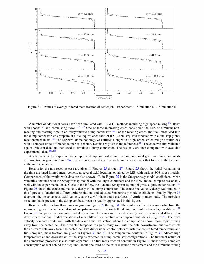
Figure 23: Profiles of average filtered mass fraction of center jet. - Experiment, – Simulation I, -.- Simulation II

A number of additional cases have been simulated with LES/FDF methods including high-speed mixing152, flowswith shocks153 and combusting flows.154–157 One of these interesting cases considered the LES of turbulent non-reacting and reacting flow in an axisymmetric dump combustor.157 For the reacting cases, the fuel introduced intothe dump combustor was propane at a fuel equivalence ratio of 0.5. Chemistry was modeled with a one-step globalreaction mechanism.158 The LES/FMDF methodology was utilized along with a high-order, structured-grid multiblockwith a compact finite-difference numerical scheme. Details are given in the references.157 The code was first validatedagainst relevant data and then used to simulate a dump combustor. The results were then compared with availableexperimental data.159,160

A schematic of the experimental setup, the dump combustor, and the computational grid, with an image of itscross-section, is given in Figure 24. The grid is clustered near the walls, in the shear layer that forms off the step andat the inflow location.

Results for the non-reacting case are given in Figures 25 through 27. Figure 25 shows the radial variations ofthe time-averaged filtered mean velocity at several axial locations obtained by LES with various SGS stress models.Comparisons of the results with data are also shown. Cd in Figure 25 is the Smagorinsky model coefficient. Meanvelocities obtained with the Smagorinsky model with the larger coefficient and the RNG model compare reasonablywell with the experimental data. Close to the inflow, the dynamic Smagorinsky model gives slightly better results.157

Figure 26 shows the centerline velocity decay in the dump combustor. The centerline velocity decay was studied inthis figure as a function of different grid resolutions and adjusted Smagorinsky model coefficients. Finally, Figure 27diagrams the instantaneous axial velocity at the z = 0 plane and isosurfaces of vorticity magnitude. The turbulentstructure that is present in the dump combustor can be readily appreciated in this figure.

Results for the reacting flow cases are given in Figures 28 through 31. The configuration differs somewhat from thenon-reacting case due to the addition of an upstream nozzle to allow better definition of inflow boundary conditions.157

Figure 28 compares the computed radial variations of mean axial filtered velocity with experimental data at fourdownstream stations. Radial variations of mean filtered temperature are compared with data in Figure 29. The axialvelocity compares quite well with the data until the last station where the computation shows more rapid mixingaway from the centerline. The predicted temperature agrees fairly well with the data downstream, but overpredictsthe upstream data away from the centerline. Two dimensional contour plots of instantaneous filtered temperature andfuel (propane) mass fraction are given in Figures 30 and 31. The temperature contours in Figure 30 indicate hightemperatures at and downstream of the step as expected in dump combustor configurations. The turbulent nature ofthe combustion processes is also quite apparent. The fuel mass fraction contours in Figure 31 show nearly completeconsumption of fuel behind the step until about one-third of the axial distance downstream and the turbulent mixing

22 of 29


Figure 24: Schematic a) of experimental setup and b)dump combustor and c) the computational grid and d) itscross-section

Figure 25: Comparison between LES and experimentaldata with different SGS models for mean axial velocity(•, experiment; solid lines, LES) a) Smagorinsky model(Cd = 0.01), b) Smagorinsky model (Cd = 0.028), c)MKEV model, d) dynamic Smagorinsky model, and e)RNG model.

and combustion of fuel beyond that station. The mixing and combustion process also penetrates significantly into thefuel core when proceeding downstream from the same station. More comparisons of the simulation results with dataand further discussions of the comparisons are given in the reference.157

IV. Concluding Remarks

This paper discusses the evolution over the past 40 years of computational methods for modeling high-speed re-acting flow fields, particularly the flow fields in scramjets and other high-speed propulsion systems. The discussionfollows from several hypersonic programs and the flight vehicles that resulted from the programs. The NASP Programand the technology program that followed provided strong motivation for advancing the computational capabilities ofthe country in both the government and private sectors. While the NASP program was not successful in developing ahypersonic vehicle, it did spawn the development of new computational capabilities. The Hyper-X Program beginningin 1995 revived high-speed computational research and development. This program culminated with the successful

23 of 29


Figure 26: Axial variations of centerline velocity

Figure 27: a) Contours of instantaneous axial velocity at the z = 0 plane and b) isosurfaces of vorticity magnitude

24 of 29


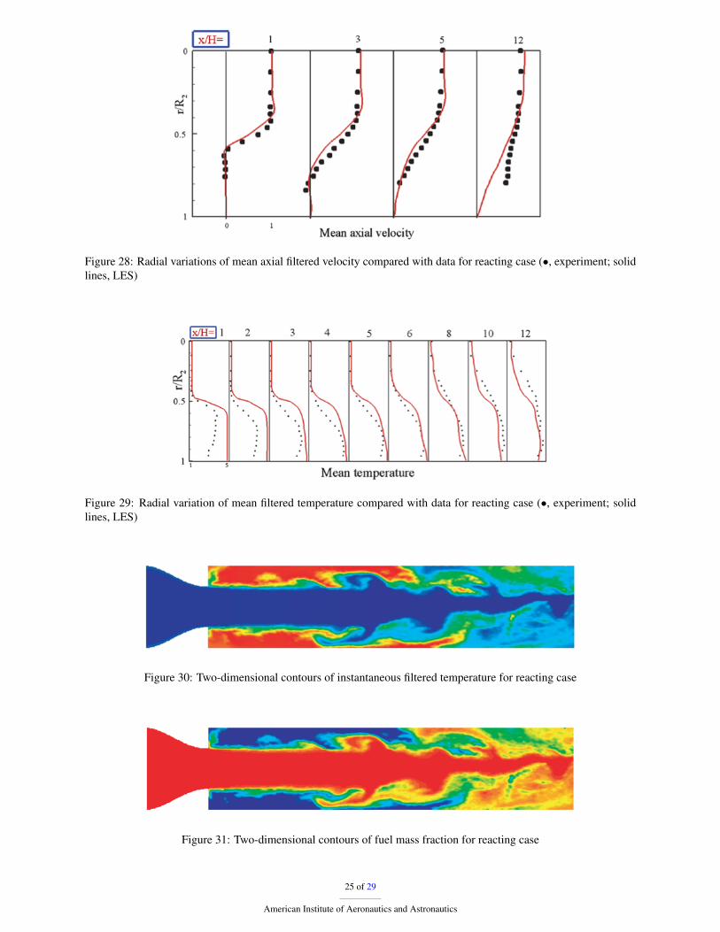
Figure 28: Radial variations of mean axial filtered velocity compared with data for reacting case (•, experiment; solidlines, LES)

Figure 29: Radial variation of mean filtered temperature compared with data for reacting case (•, experiment; solidlines, LES)

Figure 30: Two-dimensional contours of instantaneous filtered temperature for reacting case

Figure 31: Two-dimensional contours of fuel mass fraction for reacting case

25 of 29


flight of two hypersonic vehicles in 2004. A flight program is the catalyst that drives technology development andsynthesizes all of the efforts into a unified tool for development of the ultimate experiment, the flight of a hypersonicvehicle. The genesis of most of the current day state-of-the-art computational tools for scramjet research and devel-opment began with this program. This paper attempts to cover this story from NASP and Hyper-X to the present day.A number of computer programs evolved during this period of time. The programs fell into three classes, includingReynolds-averaged Navier Stokes codes, hybrid Reynolds-averaged—large-eddy simulation codes, and large-eddysimulation codes. RANS/LES codes are evolving into the workhorse codes for scramjet flow path development in thisdecade, and LES/FDF methodology appears to offer the most promise for work in the future.

References1Ferri, A., “Possible Directions of Future Research in Air Breathing Engines,” Proceedings of the Fourth AGARD Colloquium, AGARD,

1960.2Digger, D. L., “Comparison of Hypersonic Ramjet Engines with Subsonic and Supersonic Combustion,” Proceedings of the Fourth AGARD

Colloquium, AGARD, 1960.3Northam, G. B. and Anderson, G. Y., “Linear Stability Analysis of Density Stratified Parallel Shear Flows,” AIAA Paper 86-0159, 1986.4White, M. E., Drummond, J. P., and Kumar, A., “Evolution and Application of CFD Techniques for Scramjet Engine Applications,” AIAA

J. Prop. and Pwr., Vol. 3, No. 5, 1987, pp. 423–439.5Walthrup, P. J. and Billig, F. S., “Liquid Fueled Supersonic Combustion Ramjets; A Research Perspective of the Past, Present, and Future,”

AIAA Paper 86-0158, 1986.6Billig, F. S., Waltrup, P. J., and Stockbridge, R. D., “Integral-Rocket Duel-Combustion Ramjets; A New Propulsion Concept,” Journal of

Spacecraft and Rockets, Vol. 17, 1980.7Ferri, A., “Mixing Controlled Supersonic Combustion,” Annu. Rev. Fluid Mech., Vol. 5, No. x, Dec. 1973, pp. xxx–xxx.8Moretti, G., “Analysis of Two-Dimensional Problems of Supersonic Combustion Controlled by Mixing,” AIAA J., Vol. 3, 1965, pp. 223–

229.9Edelman, R. and Weilerstein, G., “A Solution of the Inviscid-Viscid Equations With Applications to Bounded and Unbounded Multicom-

ponent Reacting Flows,” AIAA Paper 69-83, 1969.10Dash, S. M., “An Analysis of Internal Supersonic Flows with Diffusion, Dissipation, and Hydrogen-Air Combustion,” NASA CR 111783,

1970.11Dash, S. M. and DelGuidice, P. D., “Analysis of Supersonic Combustion Flowfields With Embedded Subsonic Regions,” NASA CR

112223, 1972.12Elghobashi, S. E. and Spalding, D. B., “Equilibrium Chemical Reaction of Supersonic Hydrogen-Air Jets,” NASA CR 2725, 1977.13Spalding, D. B., Launder, B. E., Morse, A. P., and Maples, G., “Combustion of Hydrogen-Air Jets in Local Chemical Equilibrium,” NASA

CR 2407, 1974.14Markatos, N. C., Spalding, D. B., and Tatchell, D. G., “Combustion of Hydrogen Injected Into a Supersonic Airstream,” NASA CR 2802,

1977.15Patanker, S. V. and Spalding, D. B., “Calculation Procedure for Heat, Mass, and Momentum Transfer in Three-Dimensional Parabolic

Flows,” Int. J. Heat and Mass Transfer, Vol. 8, No. 15, 1972, pp. 1787–1806.16Evans, J. S. and Schexnayder, C. J., “Critical Influence of Finite Rate Chemistry and Unmixedness on Ignition and Combustion of Super-

sonic H2-Air Streams,” AIAA Paper 79-0355, 1979.17Dash, S. M., Sinha, N., and J., Y. B., “Implicit/Explicit Analysis of Interactive Phenomena in Supersonic Chemically Reacting Mixing and

Boundary Layer Problems,” AIAA Paper 85-1717, 1985.18MacCormack, R. W., “The Effect of Viscosity in Hypervelocity Impact Catering,” AIAA Paper 69-354, 1969.19Briley, W. R. and McDonald, H., “Solution to the Multi-Dimensional Compressible Navier-Stokes Equations,” J. Comp. Phy., Vol. 24,

1977.20Beam, R. and Warming, R. F., “An Implicit Factored Scheme for the Compressible Navier-Stokes Equations,” AIAA J., Vol. 16, No. 4,

1978, pp. 393–402.21Drummond, J. P., “Numerical Solution for Perpendicular Sonic Hydrogen Injection into a Ducted Supersonic Airstream,” AIAA J., Vol. 17,

No. 5, 1979, pp. 531–533.22Drummond, J. P., “Numerical Investigation of the Perpendicular Injector Flow Field in a Hydrogen Fueled Scramjet,” AIAA Paper 79-1482,

1979.23Drummond, J. P. and Weidner, E. H., “Numerical Study of a Scramjet Engine Flow Field,” AIAA J., Vol. 20, No. 9, 1982, pp. 1182–1187.24Drummond, J. P. and Weidner, E. H., “A Numerical Study of Candidate Transverse Fuel Injector Configurations in the Langley Scramjet

Engine,” 17th JANNAF Combustion Meeting, Hampton, VA, Sept. 1980.25Weidner, E. H. and Drummond, J. P., “Numerical Study of Staged Fuel Injection for Supersonic Combustion,” AIAA J., Vol. 20, No. 10,

1982, pp. 1426–1431.26Schetz, J. A., Billig, F. S., and Favin, S., “Flowfield Analysis of a Scramjet Combustor with a Coaxial Fuel Jet,” AIAA J., Vol. 20, No. 9,

1982, pp. 1268–1274.27Schetz, J. A., “Turbulent Mixing of a Jet in a Co-Flowing Stream,” AIAA J., Vol. 6, No. 10, 1968, pp. 2008–2010.28Schetz, J. A., Billig, F. S., and Favin, S., “Analysis of Mixing and Combustion in a Scramjet Combustor with a Coaxial Fuel Jet,” AIAA

Paper 80-1256, 1980.29Griffin, M. D., Billig, F. S., and White, M. E., “Applications of Computational Techniques in the Design of Ramjet Engines,” 6th Interna-

tional Symposium on Air Breathing Engines, ISABE, 1983, pp. 835–861.30Waltrup, P. P., Anderson, G. Y., and Stull, F. D., “Supersonic Combustion Ramjet (Scramjet) Engine Development in the United States,”

3rd International Symposium on Air Breathing Engines, ISABE, 1976, pp. 835–861.31Jenkins, D. R., Landis, T., and Miller, J., “American X-Vehicles — An Inventory — X-1 to X-50,” NASP SP 4531, 2003.32Drummond, J. P., Rogers, R. C., and Hussaini, M. Y., “A Detailed Numerical Model of a Supersonic Reacting Mixing Layer,” AIAA Paper

86-1427, 1986.33Carpenter, M. H. and Kamath, H., “Three-Dimensional Extensions to the SPARK Combustion Code,” NASP CP 5029, 1988.

26 of 29


34Carpenter, M. H., “A Generalized Chemistry Version of SPARK,” NASA CR 4196, 1988.35Chitsomboon, T. and Northam, G. B., “A 3-D PNS Computer Code for the Calculation of Supersonic Combusting Flows,” AIAA Paper

88-0438, 1988.36Chitsomboon, T., Numerical Study of Hydrogen-Air Supersonic Combustion By Using Elliptic and Parabolized Equations, Ph.D. thesis,

Old Dominion University, Norfolk, VA, 1986.37Chitsomboon, T., Kumar, A., and Tiwari, S. N., “Numerical Study of Finite-Rate Supersonic Combustion Using Parabolized Equations,”

AIAA Paper 87-0088, 1987.38Korte, J. J. and McRae, D. S., “Explicit Upwind Algorithm for the Parabolized Navier-Stokes Equations,” AIAA Paper 88-0716, 1988.39White, J. A., Korte, J. J., and Gaffney, R. L., “Flux-Difference Split Parabolized Navier-Stokes Algorithm for Nonequilibrium Chemically

Reacting Flows,” AIAA Paper 93-0534, 1993.40Guilda, T. and McRae, D., “An Accurate, Stable, Explicit, Parabolized Navier-Stokes Solver for High Speed Flows,” AIAA Paper 86-1116,

1986.41Gielda, T. P., Hunter, L. G., and Chawner, J. R., “Efficient Parabolized Navier-Stokes Solutions of Three-Dimensional, Chemically React-

ing Scramjet Flow Fields,” AIAA Paper 88-0096, 1988.42Boris, J. P., “A Fluid Transport Algorithm That Works. Computing as a Language of Physics,” International Atomic Energy Agency, IAEA,

1971, pp. 171–189.43Boris, J. P., “Flux-Corrected Transport I: SHASTA — A Fluid Transport Algorithm That Works,” J. Comp. Phy., Vol. 11, 1973, pp. 38–69.44Oran, E. S., “Numerical Simulation of Reactive Flow,” Elsever Science Publishing Company, Inc., New York, 1987, pp. 264–298.45Zalesak, S. T., “Fully Multidimensional Flux-Corrected Transport Algorithms for Fluids,” J. Comp. Phy., Vol. 31, 1979, pp. 335–362.46Oran, E. S., “Numerical Simulation of Reactive Flow,” Cambridge University Press, New York, 2001.47MacCormack, R. W., “Current Status of Numerical Solutions of the Navier-Stokes Equations,” AIAA Paper 85-0032, 1985.48Steger, J. L., “Flux Vector Splitting of the Inviscid Gasdynamic Equations with Applications to Finite-Difference Methods,” J. Comp. Phy.,

Vol. 40, 1981, pp. 263–293.49Candler, G. V. and MacCormack, R. W., “Hypersonic Flow Past 3-D Configurations,” AIAA Paper 87-0480, 1987.50Candler, G. V. and MacCormack, R. W., “The Computation of Hypersonic Ionized Flows in Chemical and Thermal Nonequilibrium,”

AIAA Paper 88-0511, 1988.51Grossman, B. and Walters, R. W., “The Computation of Hypersonic Ionized Flows in Chemical and Thermal Nonequilibrium,” AIAA

Paper 87-1117, 1987.52van Leer, B., “Flux-Vector Splitting for the Euler Equations,” Lecture Notes in Physics, Vol. 170, 1982, pp. 507–512.53Roe, P. L., “Characteristic-Based Schemes for the Euler Equations,” Lecture Notes in Physics, Vol. 18, 1986, pp. 337–365.54Anderson, W. K., Thomas, J. L., and van Leer, B., “A Comparison of Finite-Volume Flux Vector Splittings for the Euler Equations,” AIAA

Paper 85-0122, 1985.55Walters, R. W. and Dwoyer, D. L., “An Efficient Iteration Strategy Based on Upwind/Relaxation Schemes for the Euler Equations,” AIAA

Paper 85-1529-CP, 1985.56Grossman, B. and Cinnella, P., “The Development of Flux-Split Algorithms for Flows with Nonequilibrium Thermodynamics and Chemi-

cal Reactions,” AIAA Paper 88-3596, 1988.57Grossman, B. and Cinnella, P., “Flux-Split Algorithms for Flows with Nonequilibrium Chemistry and Vibrational Relaxation,” ICAM

Report 88-08-03, 1988.58Liou, M. S., van Leer, B., and Shuen, J. S., “Splitting of Inviscid Fluxes for Real Gases,” J. Comp. Phy., Vol. xx, 1988, pp. xxx–xxx.59Liou, M. S., “A Generalized Procedure for Constructing an Upwind-Based TVD Scheme,” AIAA Paper 87-0355, 1987.60Yee, H. C., “Construction of Explicit and Implicit Symmetric TVD Schemes and Their Applications,” J. Comp. Phy., Vol. 68, 1987,

pp. 151–179.61Yee, H. C. and Shinn, J. L., “Semi-Implicit and Fully Implicit Shock Capturing Methods for Hyperbolic Conservation Laws with Stiff

Source Terms,” AIAA Paper 87-1116-CP, 1987.62Yee, H. C., “Upwind and Symmetric Shock-Capturing Schemes,” NASA TM 89464, 1987.63Gnoffo, P. A., McCandless, R. S., and Yee, H. C., “Enhancements to Program LAURA for Computation of Three-Dimensional Hypersonic

Flow,” AIAA Paper 87-0280, 1987.64Gnoffo, P. A. and Green, F. A., “A Computational Study of the Flow Field Surrounding the Aeroassist Flight Experiment Vehicle,” AIAA

Paper 87-1575, 1987.65Gnoffo, P. A., Gupta, R. N., and Shinn, J. L., “Conservation Equations and Physical Models for Hypersonic Air Flows in Thermal and

Chemical Nonequilibrium,” NASA TP 2867, 1988.66Shuen, J. S. and Yoon, S., “Numerical Study of Chemically Reacting Flows Using an LU Scheme,” AIAA Paper 88-0436, 1988.67Shuen, J. S. and Yoon, S., “Three-Dimensional Simulation of an Underexpanding Jet Interacting with a Supersonic Cross Flow,” AIAA

Paper 88-3181, 1988.68Abarbanel, S. and Kumar, A., “Compact High Order Schemes for the Euler Equations,” NASA CR 181625, 1988.69Hussaini, M. Y., Salas, M. D., and Zang, T. A., “Spectral Methods for Inviscid, Compressible Flows.” Advances in Computational Tran-

sonics, edited by W. G. Habashi, Pineridge Press, New York, 1983.70Gottlieb, D. and Orszag, S. A., “Numerical Analysis of Spectral Methods, Theory, and Applications,” CBMS-NSF Regional Conference

Series in Applied Mathematics, SIAM, 1977.71Drummond, J. P., Hussaini, M. Y., and Zang, T. A., “Spectral Methods for Modeling Supersonic Chemically Reacting Flowfields,” AIAA

J., Vol. 24, No. 9, 1986, pp. 1461–1467.72Drummond, J. P., “Two-Dimensional Numerical Simulation of a Supersonic, Chemically Reacting Mixing Layer,” NASA TM 4055, 1988.73McClinton, C. R. and Hicks, J. W., “NASA Scramjet Flights to Breathe New Life into Hypersonics,” Aerospace America, Vol. 35, No. 7,

1997, pp. 40–46.74Rauch, V. L., McClinton, C. R., and Crawford, J. L., “Hyper-X: Flight Validation of Hypersonic Airbreathing Technology,” 13th Interna-

tional Symposium on Air Breathing Engines, No. 97-7024, 1997.75Saad, Y. and Schultz, M., “GMRES: A Generalized Minimum Residual Algorithm for Solving Nonsymmetric Linear Systems,” SIAM J.,

Vol. 7, No. 3, 1986, pp. 856–869.76Aerosoft, “GASP Users Manual,” Tech. Rep. 3, 1996.77Huebner, L. D. and E., T. K., “CFD Code Calibration and Inlet-Fairing Effects on a 3D Hypersonic Powered-Simulation Model,” AIAA

Paper 93-3041, 1993.

27 of 29


78Huebner, L. D. and E., T. K., “Computational and Experimental Aftbody Flow Fields for Hypersonic, Airbreathing Configurations withScramjet Exhaust Flow Simulation,” AIAA Paper 91-1709, 1991.

79Srinivasan, S., Bittner, R., and Bobskill, G., “Summary of GASP Code Application and Evaluation Effort for Scramjet Combustor Flow-fields,” AIAA Paper 93-1973, 1993.

80White, J. A., “Personal Communication,” 2011.81Kumar, A., Gnoffo, P. A., Moss, J. N., and Drummond, J. P., “Advances in Computational Capabilities for Hypersonic Flows,” AGARD

Proceedings on Future Aerospace Technology in Service to the Alliance, No. C-13, 1997.82Spalart, P. and Allmaras, S., “A One-Equation Turbulence Model for Aerodynamic Flows,” AIAA Paper 92-0439, 1992.83Wilcox, D. W., “Wall Matching , a Rational Alternative to Wall Functions,” AIAA Paper 89-0611, 1989.84Menter, F. R., “Zonal Two Equation k − ω Models for Aerodynamic Flows,” AIAA Paper 93-2906, 1993.85Menter, F. R., “Improved Two-Equation k − ω Turbulence Models for Aerodynamic Flows,” NASA-TM 103975, 1992.86Abid, R., “Evaluation of Two-Equation Turbulence Models for Predicting Trasitional Flows,” Int. J. Eng. Sci., Vol. 31, No. 6, 1993,

pp. 831–840.87Abid, R., Morrison, J. H., Gatski, T. B., and Speziale, C. G., “Prediction of Complex Aerodynamic Flows with Explicit Algebraic Stress

Models,” AIAA Paper 96-0565, 1996.88Adumitroaie, V., Colucci, P., Taulbee, D., and Givi, P., “LES, DNS, and RANS for the Analysis of High-Speed Turbulent Reacting Flows,”

NASA Report NAG 1-1122, 1994.89Girimaji, S. S., “Assumed Beta-pdf Model for Turbulent Mixing: Validation and Extension to Multiple Scalar Mixing,” Comb. Sci. Tech.,

Vol. 78, 1991, pp. 177–196.90Gaffney, R. L., White, J. A., Girimaji, S. S., and Drummond, J. P., “Modeling Temperature and Species Fluctuations in Turbulent, Reacting

Flow,” Comp. Sys. in Eng., Vol. 5, No. 2, 1994, pp. 117–133.91Srinivasan, S., “Numerical Simulation of Turbulent Flow Past a Flat Plate,” HNAG 95-2-057, 1995.92Baurle, R. A., Fuller, R. P., White, J. A., Chen, T. H., Gruber, M. R., and Nejad, A. S., “An Investigation of Advanced Fuel Injection

Schemes for Scramjet Combustion,” AIAA Paper 98-0937, 1998.93White, J. A. and Morrison, J. H., “A Pseudo-Temporal Multi-Grid Relaxation Scheme for Solving the Parabolized Navier-Stokes Equa-

tions,” AIAA Paper 99-3360, 1999.94Litton, D. K., Edwards, J. R., and White, J. A., “Algorithmic Enhancements to the VULCAN Navier-Stokes Solver,” AIAA Paper 2003-

3979, 2003.95Baurle, R. A., “Modeling of High Speed Reacting Flows: Established Practices and Future Challenges,” AIAA Paper 2004-0267, 2004.96Baurle, R. A., Tam, C. J., Edwards, J. R., and Hassan, H. A., “Hybrid Simulation Approach for Cavity Flows: Blending, Algorithm, and

Boundary Treatment Issues,” AIAA J., Vol. 41, No. 8, 2003, pp. 1463–1480.97Batten, P., Goldberg, U., and Chakravarthy, S., “Sub-Grid Turbulence Modeling for Unsteady Flow with Acoustic Resonance,” AIAA

Paper 2000-0473, 2000.98Betton, P., Goldberg, U., and Chakravarthy, S., “LNS — An Approach Towards Embedded LES,” AIAA Paper 2002-0427, 2002.99Spalart, P. R., Jou, W.-H., Strelets, M., and Allmaras, S. R., “Comments on the Feasibility of LES for Wings, and on a Hybrid RANS/LES

Approach,” 1st Air Force Office of Scientific Research International Conf. on DNS/LES, 1997.100Strelets, M., “Detached Eddy Simulation of Massively Separated Flows,” AIAA Paper 2001-0879, 2001.101Baurle, R. A., Tam, C. J., Edwards, J. R., and Hassan, H. A., “An Assessment of Boundary Treatment andAlgorithm Issues on Hybrid

RANS/LES Solution Strategies,” AIAA Paper 2001-2562, 2001.102Baurle, R. A. and Edwards, J. R., “Hybrid Reynolds-Averaged/Large-Eddy Simulations of a Coaxial Supersonic Free-Jet Experiment,”

AIAA Paper 2009-0129, 2009.103Baurle, R. A. and Edwards, J. R., “Hybrid Reynolds-Averaged/Large-Eddy Simulations of a Coaxial Supersonic Freejet Experiment,”

AIAA J., Vol. 48, No. 3, 2010, pp. 551–571.104Fan, T. C., Tian, M., Edwards, J. R., Hassan, H. A., and Baurle, R. A., “Validation of a Hybrid Reynolds-Averaged/ Large-Eddy Simulation

Method for Simulating Cavity Flameholder Configurations,” AIAA Paper 2001-2929, 2001.105Fan, T. C., Xiao, X., Edwards, J. R., Hassan, H. A., and Baurle, R. A., “Hybrid LES / RANS Simulation of a Shock Wave/ Boundary Layer

Interaction,” AIAA Paper 2002-0431, 2002.106Xiao, X., Edwards, J. R., and Hassan, H. A., “Inflow Boundary Conditions for Hybrid Large Eddy/Reynolds Averaged NavierStokes

Simulations,” AIAA J., Vol. 41, No. 8, 2003, pp. 2179–2193.107Fan, C. C., Xiao, X., Edwards, J. R., and Hassan, H. A., “Hybrid Large-Eddy/Reynolds-Averaged NavierStokes Simulations of Shock-

Separated Flows,” AIAA J. of Spacecraft and Rockets, Vol. 41, No. 6, 2004, pp. 2179–2193.108Choi, J. I., Edwards, J. R., and Baurle, R. A., “Compressible Boundary Layer Predictions at High Reynolds Number using Hybrid

LES/RANS Methods,” AIAA J., Vol. 47, No. 9, 2009, pp. 2179–2193.109Boles, J. A., Choi, J. I., Edwards, J. R., and Baurle, R. A., “Simulations of High-Speed Internal Flows using LES/RANS Models,” AIAA

Paper 2009-1324, 2009.110Boles, J. A., Edwards, J. R., and Baurle, R. A., “Large-Eddy/Reynolds-Averaged NavierStokes Simulations of Sonic Injection into Mach

2 Crossflow,” AIAA J., Vol. 48, No. 7, 2010, pp. 1444–1456.111Gieseking, D. A., Choi, J. I., Edwards, J. R., and Hassan, A. H., “Simulation of Shock / Boundary Layer Interactions Using Improved

LES/RANS Models,” AIAA Paper 2010-0111, 2010.112Edwards, J. R., Boles, J. A., and Baurle, R. A., “LES/RANS Simulation of a Supersonic Reacting Wall Jet,” AIAA Paper 2010-0370, 2010.113Gieseking, D. A. and Edwards, J. R., “Simulations of a Mach 3 Compression-Ramp Interaction using LES/RANS Models,” AIAA Paper

2011-0726, 2011.114Ziberter, I. A. and Edwards, J. R., “LES/RANS Simulations of High-Speed Mixing Processes,” AIAA Paper 2011-3423, 2011.115Peterson, D. M., Candler, G. V., and Drayna, T. W., “Detached Eddy Simulation of a Generic Scramjet Inlet and Combustor,” AIAA Paper

2009-0130, 2009.116Peterson, D. M. and Candler, G. V., “Hybrid Reynolds-Averaged and Large-Eddy Simulation of Normal Injection into a Supersonic

Crossflow,” AIAA J., Vol. 26, No. 3, 2010, pp. 533–544.117Peterson, D. M. and Candler, G. V., “Supersonic Combustor Fuel Injection Simulations Using a Hybrid RANS/LES Approach,” AIAA

Paper 2010-0411, 2010.118Barnhardt, M. and Candler, G. V., “CFD Analysis of CUBRC Base Flow Experiments,” AIAA Paper 2010-1250, 2010.

28 of 29


119Tylczak, E. B., Peterson, D. M., and Candler, G. V., “Hybrid RANS/LES Simulation of Transverse Jet in Supersonic Crossflow with LaserEnergy Deposition,” AIAA Paper 2010-4856, 2010.

120Peterson, D. M. and Candler, G. V., “Simulations of Mixing for Normal and Low-Angled Injection into Supersonic Crossflow,” AIAA J.,Vol. 49, No. 12, 2011, pp. 2792–2804.

121Peterson, D. M., Tylczak, E. B., and Candler, G. V., “Hybrid Reynolds-Averaged and Large-Eddy Simulation of Scramjet Fuel Injection,”2011.

122Tylczak, E. B., Peterson, D. M., and Candler, G. V., “Hybrid RANS/LES Simulation of Injection and Mixing in the CUBRC CombustionDuct,” 2011.

123Cutler, A. D., Diskin, G. S., Drummond, J. P., and White, J. A., “Supersonic Coaxial Jet Experiment for Computational Fluid DynamicsCode Validation,” AIAA J., Vol. 44, No. 3, 2006, pp. 585–592.

124Clifton, C. W. and Cutler, A. D., “A Supersonic Argon/Air Coaxial Jet Experiment for Computational Fluid Dynamics Code Validation,”NASA-CR 214866, 2007.

125Miles, R. B., Grinstead, J., Kohl, R. H., and Diskin, G. . S., “The RELIEF Flow Tagging Technique and its Application in Engine TestingFacilities and for Helium - Air Mixing Studies,” Meas. Sci. and Tech., Vol. 11, No. 9, 2000, pp. 1272–1281.

126Bush, R. H., Power, G. D., and Towne, C. E., “WIND: The Production Flow Solver of the NPARC Alliance,” AIAA Paper 1998-0935,1998.

127Georgiadis, N. J., Yoder, D. A., and DeBonis, J. R., “A Comparison of Three Navier-Stokes Solvers for Exhaust Nozzle Flowfields,” AIAAPaper 1999-0748, 1999.

128Nelson, C. C. and Power, G. D., “CHSSI Project CFD-7: The NPARC Alliance Flow Simulation System,” AIAA Paper 2001-0594, 2001.129MacLean, M. and Holden, M., “Validation and Comparison of WIND and DPLR Results for Hypersonic, Laminar Problems,” AIAA Paper

2004-0529, 2004.130Nelson, C. C., “An Overview of the NPARC Alliance’s WIND-US Flow Solver,” AIAA Paper 2010-0027, 2010.131Pope, S. B., “PDF Methods for Turbulent Reactive Flows,” Prog. Energy Combust. Sci., Vol. 11, 1985, pp. 119–192.132Pope, S. B., “PDF Methods for Combustion in High-Speed Turbulent Flows,” NASA-CR 199357, 1995.133Welton, W. C. and Pope, S. B., “A PDF-Based Particle Method for Compressible Turbulent Flows,” AIAA Paper 1995-0804, 1995.134Delarue, B. J. and Pope, S. B., “Application of PDF Methods to Compressible Turbulent Flows,” Phys. Fluids A, Vol. 9, 1997, pp. 2704.135Delarue, B. J. and Pope, S. B., “Calculations of Subsonic and Supersonic Turbulent Reacting Mixing Layers Using Probability Density

Function Methods,” Phys. Fluids, Vol. 10, No. 2, 1998, pp. 487–498.136Hsu, A. T., Tsai, Y. L. P., and Raju, M. S., “A PDF Approach for Compressible Turbulent Reacting Flows,” AIAA Paper 1993-0087, 1993.137Hsu, A. T. and Raju, M. S., “Application of a PDF Method to Compressible Turbulent Reacting Flows,” AIAA Paper 1994-0781, 1994.138Norris, A. T. and Hsu, A. T., “Comparison of PDF and Moment Closure Methods in the Modeling of Turbulent Reacting Flows,” AIAA

Paper 1994-3356, 1994.139Baurle, R. A. and Girimaji, S. S., “An Assumed PDF Turbulence-Chemistry Closure with Temperature-Composition Correlations,” AIAA

Paper 1999-0928, 1999.140Nik, M. B., Mohebbi, M., Sheikhi, M. R. H., and Givi, P., “Progress in Large Eddy Simlation of High-Speed Turbulent Mixing and

Reaction,” AIAA Paper 2009-0133, 2009.141Givi, P., “Filtered Density Function for Subgrid Scale Modeling of Turbulent Combustion,” AIAA J., Vol. 44, No. 1, 2006, pp. 16–23.142Poinsot, T. and Veynante, D., Theoretical and Numerical Combustion, Edwards, Philadelphia, PA, 2nd ed., 2000.143Ansari, N., Jaberi, F. A., Sheikhi, M. R. H., and Givi, P., “Filtered Density Function as a Modern CFD Tool,” Engineering Applications of

Computational Fluid Dynamics, edited by M. A. R. S. Al-Baghdadi, Int. Energy and Environment Foundation, 2011.144Givi, P., “Model Free Simulations of Turbulent Reacting Flows,” Prog. Engery Combust. Sci., Vol. 15, 1989, pp. 1–107.145Pope, S. B., “Computations of Turbulent Combustion: Progress and Challenges,” Proc. Combust. Inst., Vol. 23, 1990, pp. 591–612.146Givi, P., Sheikhi, M. R. J., Drozda, T. G., and Madnia, C. K., “Invited Review: Reliable and Affordable Simulation of Turbulent Combus-

tion,” AIAA Paper 2007-0190, 2007.147Yilmaz, S. L., Nik, M. B., Givi, P., and Strakey, P. A., “Scalar Filtered Density Function for Large Eddy Simulation of a Bunsen Burner,”

AIAA J. Prop. and Pwr., Vol. 26, No. 1, 2010, pp. 84–93.148Nik, M. B., Yilmaz, S. L., Givi, P., Sheikhi, M. R. H., and Pope, S. B., “Simulation of Sandia Flame D Using Velocity-Scalar Filtered

Density Function,” AIAA J., Vol. 48, No. 7, 2010, pp. 1513–1522.149Ansari, N., Goldin, G. M., Pisciuneri, P. H., Nik, M. B., Strakey, P. A., and Givi, P., “FDF Simulation of Swirling Reacting Flows on

Unstructured Meshes,” AIAA Paper 2011-0109, 2011.150Yilmaz, S. L., Ansari, N., Pisciuneri, P. H., Nik, M. B., Otis, C. C., and Givi, P., “Advances in FDF Modeling and Simulation,” AIAA

Paper 2011-5918, 2011.151Sheikhi, M. R. H., Givi, P., and Pope, S. B., “Frequency-Velocity-Scalar Filtered Mass Density Function for Large Eddy Simulation of

Turbulent Flows,” Phy. Fluids, Vol. 21, No. 75102, 2009, pp. 1–14.152Banaeizadeh, A., Li, Z., and Jaberi, F. A., “Compressible Scalar Filtered Mass Density Function Model for High-Speed Turbulent Flows,”

AIAA J., Vol. 49, No. 10, 2011, pp. 2130–2143.153Banaeizadeh, A., Li, Z., and Jaberi, F. A., “Large-Eddy Simulations of Compressible Turbulent Reacting Flows,” AIAA Paper 2010-0202,

2010.154Jaberi, F. A., “Large-Eddy Simulation of Turbulent Premixed Flames via Filtered Mass Density Function,” AIAA Paper 1999-0199, 1999.155Asghar, A., Jaberi, F. A., and Shih, T. I. P., “LES/FMDF of Turbulent Combustion in Complex Flow Systems,” AIAA Paper 2007-1414,

2007.156Banaeizadeh, A., Li, Z., and Jaberi, F. A., “Large-Eddy Simulation of Turbulent Combustion via Filtered Mass Density Function,” AIAA

Paper 2011-5745, 2011.157Afshari, A. and Jaberi, F. A., “Large-Eddy Simulations of Turbulent Flows in an Axisymmetric Dump Combustor,” AIAA J., Vol. 49,

No. 10, 2011, pp. 2130–2143.158Yu, J., Luo, L. S., and Girimaji, S. S., “Scalar Mixing and Chemical Reaction Simulations Using Lattice Boltzmann Method,” Int. J. of

Comp. Engr. Sci., Vol. 3, No. 1, 2002, pp. 73–78.159Gould, R. D., Stevenson, W. H., and Thompson, H. D., “Investigation of Turbulent Transport in an Axisymmetric Sudden Expansion,”

AIAA J., Vol. 28, No. 2, 1990, pp. 276–283.160Gould, R. D., Stevenson, W. H., and Thompson, H. D., “Simultaneous Velocity and Temperature Measurements in a Premixed Dump

Combustor,” AIAA J. Prop. Pwr., Vol. 10, No. 5, 1995, pp. 639–645.

29 of 29


development of methods to predict high-speed reacting flows in

Documents