Development of meat alternatives

Understanding fiber formation of vegetable proteins

Joana Lopes Pereira

Dissertação para obtenção do Grau de Mestre em

Engenharia Biológica

Júri

Presidente: Prof.ª Maria Raquel Múrias dos Santos Aires Barros (Departamento de Bioengenharia, Instituto Superior Técnico)

Orientadores: Prof.ª Marília Clemente Velez Mateus (Departamento de Bioengenharia, Instituto Superior Técnico) Dr. Ir. Fred van de Velde (NIZO food research B.V.)

Vogal: Prof.ª Maria Ângela Cabral Garcia Taipa Meneses de Oliveira (Departamento de Bioengenharia, Instituto Superior Técnico)

Setembro de 2011

“May the force be with you” Star Wars

Acknowledgements

The experience that I lived during this internship exceeded all the expectations. All the knowledge

learned in NIZO completed the five year theory learned during the course. This internship made me

realize how hard it is to work on research and that most of the times things do not go as expected. Thanks

to NIZO, I was able to have contact to a real company and gain a unique experience that will help me on

my future professional life. There are some people without whom this project couldn’t be achieved. Their

help and support were fundamental, and therefore I would like to express my sincere gratitude.

To Prof. Marília Mateus, for arranging this internship at NIZO and always be available to answer all

my questions and doubts.

To Dr. Fred van de Velde, who give me this opportunity of having my internship at NIZO. Thank you

for all the enthusiasm during the whole project and for having the time to do regular meetings just to give

me orientations and feedback on my lab work.

To Jan Klock, for always be available for all my daily questions about living in the Netherlands, for

teaching me how to work with the CLSM, and for helping me any time in the laboratory.

To Dr. Laurice Pouvreau and Dr. Thom Huppertz for always helping when I was having problems in

the laboratory.

To all the NIZO trainees, for all the lunch time at NIZO where we were always able to fit one more

person in the round table, and for the coffee time with our beloved little table.

To Tatiana Arriaga and Gonçalo Santa, who I lived with this six months, sharing not only the house

but also all the adventures. Thank you for all the amazing time spent in the kitchen, trying new recipes, for

all the ice-creams eaten at Bernardo’s and the amazing trips we did all together! This internship would not

be the same without you, for sure!

To all the friends I made in Wageningen: Giovanni, Laura, Bruno, Saxê, Aurelién, Marco, Ivy, and

the French community, who for so many times we cycled for 40 minutes just to have a barbeque with you,

or to dance at the international club. Thank you for all the nights and weekends, for all the basket-ball and

football games and for the trips, especially Lanzarote. A special thanks to Laura, for being our greatest

friend, giving us a home and food when we were too tired to go back to Ede, for all the girls dinner (with a

chocolate fountain!) and who we spent most of our time traveling.

To my friends in Portugal, Duarte Medeiros and Inês Nunes, with whom I shared my work

frustrations and joys, thanks for putting up with me and always make me smile!

Finally, a special thanks to my boyfriend Jaime Coelho, who always believed in me, despite my

clumsiness at the lab!

i

Abstract

Meat eaters are aware of the necessity of replacing meat proteins by vegetable proteins due to

sustainability issues. However they are not willing to give up the taste and flavour of meat. The goal of this

project was to develop the fiber like structures (present in meat) from vegetable proteins. The study was

focused on the relationship between vegetable proteins and a negatively charged polysaccharide in the

formation of fiber-like structures by coacervation. Three different ratios of protein/polysaccharide were

studied, 24:1, 12:1 and 6:1, being the last one the most effective in forming fibers. Different parameters on

the acidification step were also tested: the type of acid added, the stirring effect and the way of adding the

acid. The optimum conditions were achieved with adding hydrochloric acid through a pump (200 µL/min),

while stirring with a mechanic stirrer. To protect the fibers from falling apart, a cross-linking step was

tested with heat and chemical cross-linkers. The best fibers were obtained by heating at 80ºC for 30

minutes and by using 0.5% (w/w) of a food grade cross-linker. Different amounts of sodium hydroxide

were tested to neutralize the fibers. A protein matrix to involve the fibers was created, by testing different

forms of gelation: heating, adding a salt, and adding calcium chloride.

Ultimately, the project resulted in the preparation of a meat alternative (hamburger) based on the

fiber-like structures which was tasted by the project team.

Key words: Meat alternatives, vegetable proteins, polysaccharide, coacervation, fiber

microstructures.

ii

Resumo

Os consumidores de carne estão cientes da necessidade de substituir as proteínas animais pelas

vegetais devido a questões de sustentabilidade. Contudo não estão dispostos a desistir da textura e do

sabor da carne. O objectivo deste projecto foi desenvolver estruturas fibrosas (similares às presentes nos

músculos) a partir de proteínas vegetais. O estudo foi focado na relação entre proteínas vegetais e um

polissacárido na formação dessas estruturas fibrosas, através de um processo denominado coacervação.

Foram estudadas três diferentes proporções de proteína/polissacárido, 24:1, 12:1 e 6:1, sendo esta

última a mais eficaz para formar fibras. Foram também testados diferentes parâmetros no passo de

acidificação: o tipo de ácido adicionado, o efeito da agitação e o método de adição do ácido. As

condições óptimas foram obtidas com a adição de ácido clorídrico através duma bomba (200 µL/min),

agitado com um agitador mecânico. Para manter as fibras juntas foi testado um passo de cross-linking

com cross-linkers químicos e com aquecimento. As melhores fibras foram obtidas com um cross-linker

específico para produtos alimentares (0.5% w/w), e por aquecimento das fibras a 80ºC por 30 minutos.

Diferentes quantidades de hidróxido de sódio foram testadas para neutralizar o pH das fibras. Foi criada

ainda uma matriz de proteínas para envolver as fibras. Várias formas de gelatinação das proteínas foram

testadas: por aquecimento, por adição de sal, e por adição de cloreto de cálcio.

Por fim, este projecto resultou na preparação de um hambúrguer alternativo à carne, com base em

estruturas fibrosas de proteína vegetais.

Palavras chave: Alternativas à carne, proteínas vegetais, polissacárido, coacervação,

microestrutura fibrosa.

iii

Contents

Abstract ........................................................................................................................................................... i

Resumo ......................................................................................................................................................... ii

Table List ....................................................................................................................................................... v

Figures List ................................................................................................................................................... vi

Abbreviations and Symbols List .................................................................................................................... x

1 Introduction ............................................................................................................................................ 1

1.1 Meat alternatives ......................................................................................................................... 1

1.2 Coacervation ............................................................................................................................... 4

1.3 Cross-linking ................................................................................................................................ 7

1.4 Techniques .................................................................................................................................. 8

1.5 NIZO: Your food researchers .................................................................................................... 14

2 Materials and Methods ........................................................................................................................ 17

2.1 Materials and system preparation ............................................................................................. 17

2.2 Characterization of the proteins ................................................................................................ 18

2.3 Acidification ............................................................................................................................... 19

2.4 Cross-linking .............................................................................................................................. 22

2.5 Neutralization ............................................................................................................................. 23

2.6 Gelation of vegetable proteins ................................................................................................... 24

2.7 Addition of sunflower oil ............................................................................................................. 25

2.8 Large Scale ............................................................................................................................... 25

3 Results and Discussion ....................................................................................................................... 27

3.1 Characterization of the proteins ................................................................................................ 27

3.2 Acidification ............................................................................................................................... 29

3.2.1 GdL ..................................................................................................................................... 29

3.2.2 HCl ...................................................................................................................................... 35

3.2.3 Lactic acid ........................................................................................................................... 48

3.2.4 Influence of pH on the amount of protein inside the fibers ................................................. 53

3.3 Cross-linking .............................................................................................................................. 54

iv

3.3.1 Glutaraldehyde ................................................................................................................... 54

3.3.2 Food grade cross-linking agents ........................................................................................ 57

3.3.3 Heat .................................................................................................................................... 58

3.3.4 Chemical and Heat ............................................................................................................. 59

3.4 Neutralization ............................................................................................................................. 61

3.5 Gelation of vegetable proteins ................................................................................................... 65

3.5.1 Heat .................................................................................................................................... 65

3.5.2 Heat and salt ...................................................................................................................... 65

3.5.3 Heat and CaCl2 ................................................................................................................... 65

3.6 Addition of sunflower oil ............................................................................................................. 66

3.7 Large scale ................................................................................................................................ 68

4 Conclusions ......................................................................................................................................... 71

5 References .......................................................................................................................................... 73

6 Appendix .............................................................................................................................................. 75

6.1 Zetasizer .................................................................................................................................... 75

6.2 Kjeldahl Analysis ....................................................................................................................... 77

6.3 Slow acidification with GdL ........................................................................................................ 78

6.4 BCA analysis ............................................................................................................................. 80

v

Table List

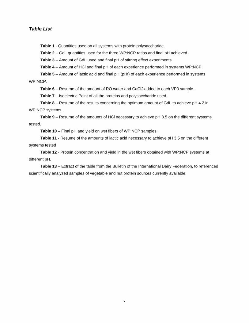
Table 1 - Quantities used on all systems with protein:polysaccharide.

Table 2 – GdL quantities used for the three WP:NCP ratios and final pH achieved.

Table 3 – Amount of GdL used and final pH of stirring effect experiments.

Table 4 – Amount of HCl and final pH of each experience performed in systems WP:NCP.

Table 5 – Amount of lactic acid and final pH (pHf) of each experience performed in systems

WP:NCP.

Table 6 – Resume of the amount of RO water and CaCl2 added to each VP3 sample.

Table 7 – Isoelectric Point of all the proteins and polysaccharide used.

Table 8 – Resume of the results concerning the optimum amount of GdL to achieve pH 4.2 in

WP:NCP systems.

Table 9 – Resume of the amounts of HCl necessary to achieve pH 3.5 on the different systems

tested.

Table 10 – Final pH and yield on wet fibers of WP:NCP samples.

Table 11 - Resume of the amounts of lactic acid necessary to achieve pH 3.5 on the different

systems tested

Table 12 - Protein concentration and yield in the wet fibers obtained with WP:NCP systems at

different pH.

Table 13 – Extract of the table from the Bulletin of the International Dairy Federation, to referenced

scientifically analyzed samples of vegetable and nut protein sources currently available.

vi

Figures List

Figure 1 – Examples of existent meat analogues: Tofu and Soy; Quorn Filet; and Seitan.

Figure 2 – Graphic with the composition of current meat alternatives.

Figure 3 – Differences between the microstructure of chicken breast and current meat alternatives,

obtained by CLSM.

Figure 4 – Steps needed to obtain a hamburger-type product.

Figure 5 – Equilibrium between glucono-delta-lactone and gluconic acid.

Figure 6 – Confocal Laser Scanning Microscopy.

Figure 7 – Schematic figure of the principle of CLSM. Image from [van de Velde and Tromp, 2002].

Figure 8 – Schematic representation of a particle and its double layer.

Figure 9 – Example of a graphic of zeta potential versus pH.

Figure 10 – Representation of the cell used to determine the zeta potential.

Figure 11 – Schematic representation of the differences between slow field reverse (A) and fast

field reverse (B).

Figure 12 – NIZO food research.

Figure 13 – Pump used to acidify the systems.

Figure 14 - Graph of the amount of vegetable protein present on each sample tested in Kjeldahl

analysis.

Figure 15 – Example of WP:NCP systems after acidification with GdL: white watery gel.

Figure 16 – General microstructure of the gels from WP:NCP systems, acidified with GDL without

stirring. Images obtained by CLSM.

Figure 17 – Fiber microstructure of WP:NCP system ratio 6:1, acidified with 0.15% (w/w) GdL

without stirring. Images obtained by CLSM.

Figure 18 - Systems WP:NCP ratio 24:1, without stirring: A) pH 5.2, B) pH 4.2. Images obtained by

CLSM.

Figure 19 - System WP:NCP ratio 24:1, with slow stirring (speed 2) at pH 5.2. Images obtained by

CLSM.

Figure 20 - System WP:NCP ratio 24:1, with slow stirring (speed 5) at pH 5.2. Images obtained by

CLSM.

Figure 21 - Systems WP:NCP ratio 6:1, shacked (speed 5): A) pH 5.4, B) pH 4.2. Images obtained

by CLSM.

Figure 22 – Graphics of the amount of acid added versus the pH of the system WP:NCP ratio 24:1

and 6:1.

Figure 23 – Graphic of the amount of acid added versus the pH of the system VP3:NCP ratio 24:1

and 6:1.

vii

Figure 24 – Three different phases of fiber formation on systems WP:NCP ratio 24:1: Before (A);

During (B); and After (C) fiber formation.

Figure 25 – Control samples of systems WP:NCP ratio 24:1 (A) and 6:1 (B). Images obtained by

CLSM.

Figure 26 – Different structures obtained during the three phases of acidification in WP:NCP

system ratio 24:1: before (A), during (B) and after (C) fiber formation. Images obtained by CLSM.

Figure 27 - Different structures obtained during the three phases of acidification in WP:NCP

system ratio 6:1:before (A), during (B) and after (C) fiber formation. Images obtained by CLSM.

Figure 28 – WP:NCP ratio 24:1 fibers, obtained by adding HCl all at once (A) and with a pump (B).

Figure 29 - Fiber microstructures obtained with the addition of HCl in WP:NCP system ratio 24:1 all

at once (A) and with a pump at the rate 200 μL/min (B). Images obtained by CLSM.

Figure 30 - WP:NCP ratio 6:1 fibers, obtained by adding HCl all at once (A) and with a pump (B).

Figure 31 – Fiber microstructures obtained with the addition of HCl in WP:NCP system ratio 6:1 all

at once (A) and with a pump at the rate 200 μL/min (B). Images obtained by CLSM.

Figure 32 – Fiber microstructures of systems WP:NCP ratio 24:1 in different stirring speeds:

Control (A), Speed 3 (B), Speed 5 (C), Speed 7 (D). Images obtained by CLSM.

Figure 33 – Fiber microstructures of systems WP:NCP ratio 6:1 in different stirring speeds: Control

(A), Speed 3 (B), Speed 5 (C), Speed 7 (D). Images obtained by CLSM.

Figure 34 – Control samples: fibers obtained with HCl and VP3:NCP systems ratio 24:1 (A) and 6:1

(B).

Figure 35 – Fiber microstructures on control samples with VP3:NCP systems ratio 24:1 (A) and 6:1

(B). Images obtained by CLSM.

Figure 36 - VP3:NCP ratio 24:1 (A) and 6:1 (B) fibers, obtained by adding HCl all at once.

Figure 37 - Fiber microstructures obtained by adding HCl all at once on samples with VP3:NCP

systems ratio 24:1 (A) and 6:1 (B). Images obtained by CLSM.

Figure 38 - Fiber microstructures obtained by adding HCl with a pump on samples with VP3:NCP

systems ratio 24:1 (A) and 6:1 (B). Images obtained by CLSM.

Figure 39 – Graphic of the amount of acid added versus the pH of the system WP:NCP ratio 24:1

and 6:1.

Figure 40 – Graphic of the amount of acid added versus the pH of the system VP3:NCP ratio 24:1

and 6:1.

Figure 41 - Control sample of system WP:NCP ratio 24:1 after lactic acid acidification. Image

obtained by CLSM.

Figure 42 - Fiber microstructures obtained by adding lactic acid in WP:NCP systems ratio 24:1: all

at once (A) and with a pump (B). Images obtained by CLSM.

Figure 43 - Fiber microstructures obtained by adding lactic acid in WP:NCP systems ratio 6:1:

control (A) and with a pump (B). Images obtained by CLSM.

viii

Figure 44 – Example of the texture of the fibers obtained after VP3:NCP ratio 24:1 acidification with

lactic acid (A) and its microstructure obtained by CLSM (B).

Figure 45 - Control sample of system VP3:NCP ratio 6:1 acidified with lactic acid (A) and its

microstructure obtained by CLSM (B).

Figure 46 - Fiber microstructures obtained by adding lactic acid in VP3:NCP systems ratio 6:1: all

at once (A) and with a pump (B). Images obtained by CLSM.

Figure 47 – Example of one plate of BCA ready to be analyzed

Figure 48 – Fibers obtained from VP3:NCP and HCl: control (A) and cross-linked with

glutaraldehyde (B).

Figure 49 - Fiber microstructures obtained in VP3:NCP systems ratio 6:1 and HCl: control (A) and

cross-linked with glutaraldehyde (B). Images obtained by CLSM.

Figure 50 – Fibers obtained from VP3:NCP and lactic acid: control (A) and cross-linked with

glutaraldehyde (B).

Figure 51 - Fiber microstructures obtained in VP3:NCP systems ratio 6:1 and lactic acid: control (A)

and cross-linked with glutaraldehyde (B). Images obtained by CLSM.

Figure 52 - Fibers obtained from VP3:NCP and HCl, cross-linked with FGC1 (A) and its

microstructure obtained by CLSM (B).

Figure 53- Fibers obtained from VP3:NCP and HCl, cross-linked with FGC2 (A) and its

microstructure obtained by CLSM (B).

Figure 54 - Fibers obtained from VP3:NCP and HCl, cross-linked by heating (A) and its

microstructure obtained by CLSM (B).

Figure 55 - Fibers obtained from VP3:NCP and HCl, cross-linked with glutaraldehyde and heating

(A) and its microstructure obtained by CLSM (B).

Figure 56 - Fibers obtained from VP3:NCP and lactic acid, cross-linked with glutaraldehyde and

heating (A) and its microstructure obtained by CLSM (B).

Figure 57 - Fibers obtained from VP3:NCP and HCl, cross-linked with FGC1 and heating (A) and

its microstructure obtained by CLSM (B).

Figure 58 - Fibers obtained from VP3:NCP and HCl, cross-linked with FGC2 and heating (A) and

its microstructure obtained by CLSM (B).

Figure 59 - Differences on the yield in wet fibers of VP3:NCP ratio 6:1 before and after

neutralization.

Figure 60 – Graphic of the protein yield in fibers of VP3:NCP ratio 6:1 before and after

neutralization.

Figure 61 - Graphic of the water holding capacity of fibers VP3:NCP ratio 6:1 before and after

neutralization.

Figure 62 – Example of fibers from VP3:NCP systems 6:1 ratio, obtained after adding NaOH.

Figure 63 –Graphic with results of pH versus the amount of NaOH in 125g of system with

VP3:NCP ratio 6:1

ix

Figure 64 - Fiber microstructures of VP3:NCP systems ratio 6:1 with 5% (w/w) sunflower oil.

Images obtained by CLSM.

Figure 65 – Fibers obtained of VP3:NCP systems ratio 6:1 with 10% (w/w) sunflower oil (A) and its

microstructure (B). Image obtained by CLSM.

Figure 66 – Large scale test, fiber cross-linked with FGC2 with 2% (w/w) egg white protein matrix:

before (A) during (B) and after fry (C).

Figure 67 – Large scale test, fiber cross-linked with 1% (w/w) heat and compressed, with egg white

protein matrix: before (A) and after fry (B and C).

Figure 68 - Graphic of zeta potential variation of WP along a range of pH.

Figure 69 - Graphic of zeta potential variation of VP1 along a range of pH.

Figure 70 – Graph of zeta potential variation of VP3 along a range of pH.

Figure 71 - Graphic of zeta potential variation of VP4 along a range of pH.

Figure 72 - Graphic of zeta potential variation of NCP along a range of pH.

Figure 73 – Acidification profile for systems WP:NCP ratio 24:1 at 25ºC, using different GdL

concentrations.

Figure 74 - Acidification profile for systems WP:NCP ratio 12:1 at 25ºC, using different GdL

concentrations.

Figure 75 - Acidification profile for systems WP:NCP ratio 6:1 at 25ºC, using different GdL

concentrations.

Figure 76 - Graphic of the final pH achieved for each concentration of GdL, for WP and NCP ratio

of 24:1 at 25ºC.

Figure 77- Graphic of the final pH achieved for each concentration of GdL, for WP and NCP ratio of

12:1 at 25ºC.

Figure 78 - Graphic of the final pH achieved for each concentration of GdL, for WP and NCP ratio

of 6:1 at 25ºC.

Figure 79 – Graphic of BCA results, with the standard curve and the interpolations of the protein

concentrations in the experience of “influence of pH on the amount of protein inside the fibers”.

Figure 80 – BCA protocol followed.

x

Abbreviations and Symbols List

BCA - Bicinchoninic Acid Analysis

CLSM – Confocal Laser Scanning Microscopy

FGC – Food Grade Cross-linker

GdL - Glucono delta-lactone

HCl - Hydrochloric acid

NCP – Negatively Charged Polysaccharide

OD – Optical density

pI – Isoelectric Point

RO - Reverse Osmosis

VP – Vegetable Protein

WP - Whey Protein

1

1 Introduction

1.1 Meat alternatives

Meat and poultry are the basis of the daily diet of people around the world. Eating 160g of meat per

day is recommended as part of a healthy and balanced diet [1]. Meat consumption is also becoming more

and more important in oriental countries, such as Japan and China. For example, 30 years ago meat was

a luxury, only brought for special occasions. Now sales of meat in China are rising 10% each year,

making for a booming meat market [2]. In the United States of America, the total meat and poultry

production in 2010 reached more than 41.8 billion kg [1].

With the increase of global demand for meat products over the years, awareness of the

environmental damage that this industry causes also increased. Modern meat production uses enormous

amounts of energy, pollutes water supplies and creates greenhouse gases[3]. People are getting more

concerned about all these problems and the overexploitation and mistreatment of animals. All this is

becoming to play an important role in the decision on which products to buy. Many people are choosing to

become vegetarians, changing their meat-eating habits into new products such as soy, tofu or seitan.

However these products only give the customers the proteins they need for a meal, letting the taste,

juiciness and texture of a good steak apart. For that reason people do not want to give up on meat

despite their environmental concerns.

Apart from the environmental issues, sustaining animals take time and a lot of costs are involved.

Besides the food associated costs, there are also costs with veterinary care (such as mandatory vaccines

and veterinary inspections), workers, slaughterhouses, packing and distribution. With the growing

consumption of meat the demand for grains raised, since they represent around 70% of animal food. This

is contributing to the increase of grain prices [4]. In Brasil for example, some animal farmers are starting

to lose money with their animals due to this increase [5].

It is then important to create meat alternatives for meat eaters that are not only similar in texture

taste and mouth feel to the actual meat but also economically viable. Consumers ask for sustainable use

of resources, including food proteins. Animal proteins, including meat and meat products, are less

sustainable compared to vegetable proteins. However consumers do not change their habits towards

eating more vegetables. Meat fulfills several of people’s needs: it is the major source of protein nutrition

and it has a good taste and texture. Also eating meat is a cultural issue and it is in everyone habits.

2

Some of the meat analogues that are currently on the marker, such as Quorn Filet, Alpro Soya or

Hamburger Tivall (Figure 1), have a really high content of lipids (Figure 2). When comparing their

microstructure with actual meat, the differences are striking. Meat is characterized by well-defined

muscular fiber structures, whereas the meat analogues are composed by lumps of vegetable proteins

(Figure 3).

Figure 1 – Examples of existent meat analogues: Tofu and Soy; Quorn Filet; and Seitan.

Figure 2 – Graphic with the composition of current meat alternatives.

0

2

4

6

8

10

12

14

16

18

proteins Sugars Lipids Fiber

Quorn Filet

Valees Mediterraan

Alpro Soya

Tivall Hamburger

3

Figure 3 – Differences between the microstructure of chicken breast and current meat alternatives, obtained by CLSM.

In order to get the meat fibrous texture, the solution may rely on structuring vegetable proteins into

fibers, creating fibrous structures for the essential meat bite experience. In this way it is also possible to

have control over the juiciness and texture of the meat alternative. The fibrous structure can be achieved

by combining vegetable proteins with a polymer.

As whey proteins have been more studied and are easier to work with than vegetable proteins

(more soluble), the experiments in this project were first performed with whey protein (WP). WP are

globular proteins present in milk, mainly composed of β-lactoglobulin, α-lactalbumin, bovine serum

albumin, immunoglobulin and several minor proteins and enzymes.

The final objective of this project was not only to create fibers but also to give them the familiar

hamburger shape. One way of obtaining this desired shape is by involving the fibers with a protein matrix.

This gel can be obtained with vegetable proteins in presence of a salt. By heating the mixture of fibers

and protein solution, a solid hamburger-type product with fiber texture is obtained (Figure 4). To improve

the taste, sunflower oil can be added, either to the protein solution, or directly into the fibers.

Figure 4 – Steps needed to obtain a hamburger-type product.

Protein Solution

Wet Fibers

Mix / Shape Heat Hamburger Bake

4

1.2 Coacervation

Proteins and polysaccharides are biopolymers widely present in living organisms. They can be

naturally associated in order to maintain cell integrity (membranes, organelles) or induce cell division

(histones / DNA complexes, enzyme catalysis) [Menger, 2002], but they can also be incompatible,

participating in cell partition [Turgeon et al, 2003].

In food engineering, proteins and polysaccharides play a key role in the structuration and

stabilization of food systems, through their gelling, thickening, and surface stabilizing functional properties

[Tolstoguzov, 1991]. The final structure, texture and stability of food materials are determined by the

interactions between the different compounds.

A diluted non-interactive biopolymer mixture of proteins and polysaccharides may be co-soluble.

However in most cases they are unstable and phase separation can be achieved in two distinct ways.

The interactions between the biopolymers can be repulsive in nature and so the system forms two

phases, each of them enriched with one biopolymer – segregation. On the other hand the interactions can

be attractive (usually through electrostatic interactions like when biopolymers have oppositely charged

groups) and then the system exhibits a two-phase region with the two biopolymers concentrated in one

phase – coacervation [Schmitt et al, 1998].

Coacervation was first discovered by Tiebackx in 1911. It results from weak attractive and

positive/negative interactions between biopolymers, giving rise to the formation of soluble or insoluble

complexes. The first theoretical explanation of the coacervation phenomenon was presented by

Bungenberg de Jong and Kruyt. They described it as “a liquid which had lost its free mobility to a certain

degree” [Bungenberg de Jong and Kruyt, 1929].

The Tainaka theory is the most recent model developed for complex coacervation, and is an

adaptation of the Veis – Aranyi theory [Veis and Aranyi, 1960]. Veis and Aranyi developed a theory for

coacervation, considering it as a two-step process rather than a spontaneous one. First, the gelatins

spontaneously aggregate by electrostatic interaction to form neutral aggregates of low configurational

entropy. Then these aggregates slowly rearrange to form the coacervate phase. The mechanism is driven

by the gain in configurational entropy resulting from the formation of a randomly mixed coacervate phase.

Veis and Aranyi considered that the molecules were not randomly distributed in both phases, but that ion-

paired aggregates are present in the dilute phase.

Tainaka theory differentiates from the Veis – Aranyi model in one main point. He claims that the

aggregates, present in both the dilute and concentrated phase, are formed without specific ion pairing

[Tainaka, 1980]. The biopolymer aggregates present in the initial phase condense to form a coacervate.

According to Tainaka, the driving forces for phase separation are the electrostatic and the attractive force

between the aggregates, which become stronger when the molar mass and the charge density of the

polymers increase. Charge density and molar mass of the polymers should fall within a critical range for

coacervation to occur. If the charge density or molar mass of the polymer becomes higher than the critical

5

range, then a concentrated gel or a precipitate, induced by the long-range attractive forces among the

aggregates, will be formed. On the other hand, for charge densities or molar mass below the range, short

range repulsive forces will stabilize the dilute solution and coacervation will not occur. The Tainaka theory

is general and is applicable to both high and low charge density systems. It provides an adequate

explanation of the complex coacervation process for a large number of systems.

Most of the polymers used on the food field and negatively charged. So the systems must have

positively charged proteins. The opposite is not yet proved that forms fibrous structures.

Parameters that influence coacervation

The interactions that originates coacervation can be electrostatic, Van der Waals or hydrophobic

interactions and even hydrogen bonding. Various physico-chemical parameters influence these

interactions and thus the complex formation. Electrostatic interactions are the strongest and therefore

preferred.

The pH plays a key role in the strength of electrostatic interaction since it determines the charge

density of the proteins (in the amino and carboxylic groups). The maximum coacervation yield is therefore

obtained below the pI of the protein [Schmitt et al, 1998]. For that pH the two biopolymers carry opposite

net charges, resulting in a maximum electrostatic attraction. The major component of WP is

β-lactoglobulin (52%) and its pI 5.2 [Vasbinder, 2002]. Having this value in mind and to guaranty that

coacervation occurs, the acidification pH was established at 4.2.

From the yield in wet fibers the amount of water retained can also be deduced. This yield is an

important tool to understand how much fibers can be obtained from a certain initial amount of biopolymer

mixture.

To achieve coacervation, acidification can occur in a slow or quick way. One would think that with

slow acidification proteins would have time to organize themselves in the long chains of the polymer. This

would result in a very well defined fiber microstructure. For this slow acidification, glucono-delta-lactone

(GdL) is used. GdL is a neutral cyclic ester of gluconic acid (Figure 5), produced by an aerobic

fermentation of a carbohydrate source. When added to an aqueous solution, GdL dissolves rapidly, then

it progressively hydrolyses into gluconic acid, a weak acid [Jungbunzlauer, 2008]. GdL is commonly found

in honey and fruit juices. For the quick acidification a strong and weak acid can be used, for example

hydrochloric acid (HCl) and lactic acid, respectively.

Figure 5 – Equilibrium between glucono-delta-lactone and gluconic acid.

6

Another important parameter is the protein-to-biopolymer ratio. Each system has a specific ratio

were maximum coacervation yield is achieved. For ratios where one of the biopolymers is in excess,

soluble complexes are obtained due to the presence of nonneutralized charges which decrease the

turbidity. Otherwise, when the polysaccharide or the protein are in excess in the solution, no coacervation

occurs because of the low energetic interest of concentrating the biopolymers into coacervates if the

concentration in solution is already high [Schmitt et al, 1998]. For this project, three different protein-

polymer ratios were tested: 24:1, 12:1 and 6:1.

Coacervation in Industry

Protein-biopolymer complexes have many uses in industry. They can be used in food,

biotechnology, medicine, pharmacy or cosmetic. Three important applications of this kind of complexes

seem to retain higher interest than the others [Schmitt et al, 1998].

Complex coacervation can be applied to the purification of macromolecules as coacervation is a

reversible process. The purification of macromolecules through chromatographic or membrane filtration

techniques is generally expensive. This is often due not only to the lack of selectivity and efficiency of the

methods, but also due to the use of solvents. In contrast, the use of complex coacervation in the

purification of biopolymers is a simpler and cheaper method, since the cost depends practically only on

the price of the biopolymers.

Interfacial properties of the complexes can be used in the microencapsulation of active molecules.

Microencapsulation result from the ability of protein-polysaccharide complexes to form a solid film around

emulsion droplets containing the product to be encapsulated and also the possibility of entrapping solvent

molecules into the coacervate (microgels) [Thies, 1982].

Finally, complexes can be used as new materials, as ingredients in food formulation, or as

biomaterials in food protection and packaging. In the last 30 years the use of complexes in the food

industry increased, especially in North American countries. The biological nature of proteins and

polysaccharides is one of the main advantages in using them to form complexes. They can be used in

products which are directly in contact with the organism, with limited allergical risks [Schmitt et al, 1998].

Also these macromolecules are entirely biodegradable, which limits environmental hazards. The ways of

producing new ingredients and, consequently, new food products appears wide as the possibility of using

coacervation complexes from these two biopolymers has been discovered [Dziezak, 1989]. One of the

many applications is the meat analogues. The first patent application was proposed by Tolstoguzov et al

[Tolstoguzov et al, 1974]. However this patent used animal-derived proteins (casein). This project has the

goal of developing the fiber-like structures from vegetable proteins only, which can serve as the basis for

the creation of meat alternatives.

7

1.3 Cross-linking

Cross-links are the bonds that link one polymer chain to another. This can be achieved by using a

chemical or physical agent that links the proteins to the polymer. When the polymer chains are linked they

lose some of their ability to move as individual polymer chains (a liquid polymer can be turned into a solid

or a gel). After coacervation, the complexes (fibers in this project) remain loose in the remaining liquid.

The step of cross-linking is intended to aggregate the fibers all together, turning the links between protein

and polymer stronger. In this way, cross-linking is expected to protect the fibers when returning to neutral

pH, since these tend to reverse the coacervation process.

Cross-links can be formed by chemical reactions that are initiated by heat, pressure, change in pH,

radiation or with the help of chemicals called cross-linking reagents. Cross-links by chemicals are very

stable mechanically and thermally, so once formed are difficult to break. In this project heat and two

different cross-linking reagents were tested.

The first cross-linking reagent used was glutaraldehyde, which is and organic compound

[CH2(CH2CHO)2]. Glutaraldehyde is often used as an amine-reactive cross-linker. It is mainly used in

industrial water treatment and as a chemical preservative. However this reagent is toxic, causing severe

eye, nose throat and lung irritations. This cross-linking reagent was only used to reject the impossibility of

cross-linking, i.e. if cross-linking did not take place with glutaraldehyde, it would probably never work with

any other cross-linking reagent. In this project food grade alternatives were used.

8

1.4 Techniques

Confocal Laser Scanning Microscopy

In order to obtain a good bite experience on the meat alternative, it is crucial to obtain a similar

microstructure to the actual meat. Clear relationships between microstructure, texture and perception

have been described for mouthfeel attributes, such as hardness (or firmness), crumbliness, separation (or

juiciness) and spreadable [Foegeding et al, 2011].

Confocal Laser Scanning Microscopy (CLSM) is a powerful tool to visualize the microstructure of

food products as well as the special distribution of ingredients therein [van de Velde and Klok, 2011]. The

key feature of confocal microscopy is its ability to acquire in-focus images from selected depths. This way

the laborious process of slicing the sample is avoided (non-invasive technique). Another advantage is the

ability of identifying different ingredients within a product, by combining different lasers and fluorescent

dyes.

The CLSM used in this project was a Leica TCS SP5. It is composed by the microscope itself, the

scanner, the computer with two screens and a panel (Figure 6).

Figure 6 – Confocal Laser Scanning Microscopy.

In the CLSM a laser beam passes through a light source opening (pinhole) and then is focused by

an objective lens into a small focal volume within or on the surface of the sample (Figure 7). The pinhole

rejects all out of focus light so that focusing is done on one point of the sample. As mentioned before,

fluorescent dyes are needed since this technique only works when the sample itself serves as a light

source. Scattered and reflected laser light, as well as any fluorescent light from the illuminated spot, is

then re-collected by the objective lens. A semi-transparent mirror separates off some portion of the light

into the detection apparatus. After passing a pinhole the light intensity is detected by a photodetection

device, transforming the light signal into an electrical one that is recorded by a computer. As most of the

9

returning light is blocked by the pinhole, the resulting image is sharper than those from conventional

fluorescence microscopy techniques. The distance between the objective and the specimen determines

the depth of the scan in the sample. Three-dimensional images are created by sequencing a large

number of two-dimensional figures of one sample [van de Velde and Tromp, 2002].

Figure 7 – Schematic figure of the principle of CLSM. Image from [van de Velde and Tromp, 2002].

For proteins, the dye used is Rhodamine B. In the images obtained, the bright areas are rich in

protein, whereas the darker areas contain less protein. An example was already presented on Figure 3,

where chicken breast and a current meat alternative were dyed with rhodamine.

Through this dissertation, most of the images obtained with CLSM are presented in gray scale, in

order to have a better resolution of the microstructures.

10

Zetasizer

To obtain the pI of the proteins used on this project, the zeta potential was measured with the

equipment Zetasizer Nano series, from Malvern Instruments.

The growth of a net charge at the particle surface affects the distribution of ions in the surrounding

interfacial region, resulting in an increased concentration of counter ions (ions of opposite charge to that

of the particle) close to the surface. So an electrical double layer exists around each particle (Figure 8).

The liquid layer surrounding the particle also exists as two parts; an inner region, called the Stern

layer, where the ions are strongly bound and an outer, diffuse, region where they are less firmly attached.

Within the diffuse layer there is a notional boundary inside which the ions and particles form a stable

entity. When a particle moves (e.g. due to gravity), ions within the boundary move with it, but any ions

beyond the boundary do not travel with the particle. This boundary is called the surface of hydrodynamic

shear or slipping plane. The potential that exists at this boundary is known as the Zeta potential.

Figure 8 – Schematic representation of a particle and its double layer.

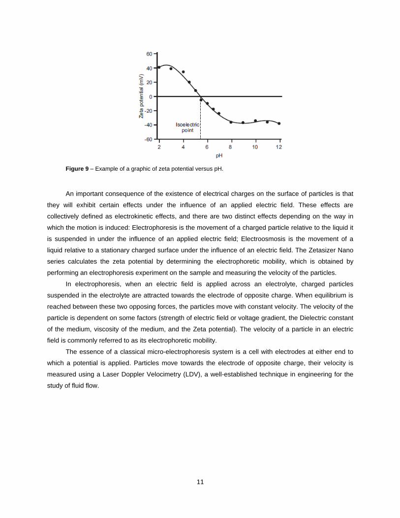
The most important factor that affects zeta potential is pH. A zeta potential value on its own without

a quoted pH is a virtually meaningless number. A zeta potential versus pH curve will be positive at low pH

and lower or negative at high pH (Figure 9). The point where the plot passes through zero zeta potential

is called the Isoelectric point (pI) and is very important from a practical consideration. It is normally the

point where the colloidal system is least stable.

Stem potential

Surface potential

Zeta potential

Diffuse Layer

Distance from particle surface

-100

mV

0

Stem Layer

Electrical double layer

Slipping plane

Particle with negative surface charge

11

Figure 9 – Example of a graphic of zeta potential versus pH.

An important consequence of the existence of electrical charges on the surface of particles is that

they will exhibit certain effects under the influence of an applied electric field. These effects are

collectively defined as electrokinetic effects, and there are two distinct effects depending on the way in

which the motion is induced: Electrophoresis is the movement of a charged particle relative to the liquid it

is suspended in under the influence of an applied electric field; Electroosmosis is the movement of a

liquid relative to a stationary charged surface under the influence of an electric field. The Zetasizer Nano

series calculates the zeta potential by determining the electrophoretic mobility, which is obtained by

performing an electrophoresis experiment on the sample and measuring the velocity of the particles.

In electrophoresis, when an electric field is applied across an electrolyte, charged particles

suspended in the electrolyte are attracted towards the electrode of opposite charge. When equilibrium is

reached between these two opposing forces, the particles move with constant velocity. The velocity of the

particle is dependent on some factors (strength of electric field or voltage gradient, the Dielectric constant

of the medium, viscosity of the medium, and the Zeta potential). The velocity of a particle in an electric

field is commonly referred to as its electrophoretic mobility.

The essence of a classical micro-electrophoresis system is a cell with electrodes at either end to

which a potential is applied. Particles move towards the electrode of opposite charge, their velocity is

measured using a Laser Doppler Velocimetry (LDV), a well-established technique in engineering for the

study of fluid flow.

12

Figure 10 – Representation of the cell used to determine the zeta potential.

The walls of the capillary cell carry a surface charge so the application of the electric field needed

to observe electrophoresis causes the liquid adjacent to the walls to undergo electroosmotic flow.

However, in a closed system the flow along the walls must be compensated for by a reverse flow down

the center of the capillary. There is a point in the cell at which the electroosmotic flow is zero - where the

two fluid flows cancel. If the measurement is then performed at this point, the particle velocity measured

will be the true electrophoretic velocity. This point is called the stationary layer and is where the two laser

beams cross; the zeta potential measured is therefore free of electroosmotic errors.

However, the measurement takes place the middle of the cell, rather than at the stationary layer.

This is because the measurement zone is further from the cell wall, so reduces the chance of flare from

the nearby surface.

So the experiment consists of two measurements for each Zeta potential measurement, one with

the applied field being reversed slowly and a second with a rapidly reversing applied field (Figure 11).

The first reversal is applied to reduce the polarization of the electrodes that is inevitable in a

conductive solution. The field is usually reversed about every 1 second to allow the fluid flow to stabilize.

If the field is reversed much more rapidly, it is possible to show that the particles reach terminal velocity,

while the fluid flow due to electroosmosis is insignificant. This means that the mobility measured during

this period is due to the electrophoresis of the particles only, and is not affected by electroosmosis. The

mean zeta potential that is calculated by this technique is therefore very robust, as the measurement

position in the cell is not critical

Figure 11 – Schematic representation of the differences between slow field reverse (A) and fast field reverse (B).

Significant fluid flow Insignificant fluid flow

A) B)

13

Bicinchoninic Acid and Kjeldahl Analysis

The vegetable proteins were selected depending on their solubility. For that, Bicinchoninic Acid

Analysis (BCA) and Kjeldahl analysis were used.

BCA is a highly sensitive colorimetric assay that can quantify the amount of proteins present in a

solution. The total protein concentration is exhibited by a color change of the sample solution from green

to purple in proportion to protein concentration. The amount of protein in the sample is then quantified by

measuring the absorbance at 562 nm and comparing with protein solutions with known concentrations.

In more detail, the BCA combines the reduction of Cu2+

to Cu1+

by protein in an alkaline medium

with the highly sensitive and selective colorimetric detection of the cuprous cation by bicinchoninic acid.

The reaction that leads to BCA color formation is strongly influenced by four amino acid residues in the

amino acid sequence of the protein: cysteine, cystine tyrosine and tryptophan. However, unlike the

Coomassie dye-binding methods, the universal peptide backbone also contributes to color formation,

helping to minimize variability caused by protein compositional differences [Smith et al, 1985].

Kjeldahl analysis is a method to determine the amount of nitrogen present in a sample. It is used

on a large variety of samples, such as meat, grains, waste water, and soil, among others. Even though

Kjeldahl is the internationally-recognized method for estimating protein content in food, it does not give a

measure of true protein content, as it measures nonprotein nitrogen in addition to the nitrogen in proteins.

This is evident by the 2007 pet food incident and 2008 Chinese milk powder scandal, where melamine (a

nitrogen-rich chemical) was added to raw materials to fake high protein contents [6].

The method consists of heating the sample with concentrated sulfuric acid, which decomposes the

organic sample by oxidation, to liberate the reduced nitrogen as ammonium sulfate. This solution is then

distilled with sodium hydroxide to convert the ammonium salt into ammonia. The amount of ammonia is

then determined by titration. The quantity of nitrogen in the sample can be calculated from the quantified

amount of ammonia, by applying a correction factor that is specific for each different protein (Chapter

6.2).

14

1.5 NIZO: Your food researchers

NIZO food research is one of the most advanced and independent contract research companies in

the world. With 200 employees, it successfully assists food and ingredient companies to make better

foods and be more profitable by developing and applying competitive technologies to support innovation

(flavor, texture, health), cost reduction (process efficiency, ingredient replacement, test productions)

and responsible entrepreneurship (food safety & quality, sustainable processing, evidence based health

claims).

Figure 12 – NIZO food research.

In 1948, NIZO was established by the joint Dutch dairy industry. First as a quality and food safety

control, institute NIZO soon also worked on innovations. This resulted for example in the development of

famous cheeses (Leerdammer, Proosdij, Kernhemmer and Parrano), which were made famous brands by

their customers.

A new Pilot Plant was built in 1974, underlining the importance for NIZO to translate laboratory

results to industrial level. The food grade Pilot-Plant accessible for third parties (largest in Europe and

one of largest in the world) is now also used for test productions and tolling of high value ingredients.

Changing its name to NIZO food research in the early 1990s – emphasizing the widening of

scope - NIZO since then developed and applied technologies for improvements in a wide range of food

products.

In 2003 NIZO food research became a BV (private company). Since then NIZO not only works on

confidential research projects for the international food, beverage and ingredient industries but also for

the international dairy industries.

15

In 2005, offices were established in the UK, France and the USA, and in 2007 a new office was

opened in Japan.

In the year of NIZOs 60th anniversary (2008) the new Application Centre with industrial kitchen

facilities was opened and is available for product oriented research or to develop new food concepts with

the assistance of scientists or a chef.

In 2009 the management team acquired total ownership of NIZO food research B.V. underlining the

independent status of NIZO. Already 15 years ago, the Dutch dairy industry as previous owners

challenged NIZO to develop into a modern and financially independent organization. As a consequence,

NIZO expanded its activities beyond the dairy horizon into the general food industry while also expanding

activities outside The Netherlands. The Management Buy Out was just a logical conclusion of that

development.

The basis of NIZO’s success in the market is a thorough knowledge of ingredients, their

modifications and their interactions in consumer products. Thorough knowledge of food chemistry,

microbiology and physics, life sciences and the implication of processing on the products’ functionality

enable NIZO to create, analyze and understand food with all its functional benefits. NIZO is ISO

9001:2008 certified.

NIZO’s Vision

Nowadays consumers are more demanding, aware and are looking for convenience. They want a

larger selection of healthy and responsible food. On society, level rules and regulations about food are

getting more essential. The industry, on their side, need to distinguish themselves in an effective and

efficient way. However they cannot have all the knowledge in house to meet the innovation requirements.

Independent provision of knowledge and development of technologies that can be applied to improve

functional benefits and processes in food shall therefore play a crucial role.

NIZO’s Mission

To improve functional consumer benefits (flavor, texture, health and food safety) and processes in

foods.

To be the preferred technology provider for the food industry worldwide by developing and applying

innovative technologies.

Experience the joy of innovation and the application of technology for the industry to improve the

quality of foods and ingredients, thereby increasing the quality of life.

16

17

2 Materials and Methods

All the laboratorial experiments were performed at NIZO’s laboratories, in Flavour and Texture

Department, during the months between March 2011 and August 2011.

In order to obtain accurate results all the systems were prepared following the same protocol.

2.1 Materials and system preparation

The materials used in this project were vegetable proteins (called VP1 to 4), whey protein (WP),

negatively charged polysaccharide (NCP), glucono delta-lactone (GdL), hydrochloric acid (HCl), lactic

acid, sodium hydroxide (NaOH), glutaraldehyde, food grade cross-linker (FGC 1 and 2), sodium azide

(NaN3), sodium chloride (NaCl), calcium chloride (CaCl2), sunflower oil and egg white protein.

Every stock solution was prepared a day before the experiments. VP 1, 2 and 4 stock solutions

were prepared by adding the powder to reverse osmosis (RO) water in 10% w/w, stirred at least 2 hours

at room temperature, stirred overnight at 5ºC and centrifuged for 15 minutes at 2000 rpm, collecting the

supernatant (≈6% protein w/w). VP 3 stock solution was prepared by adding the powder to RO water at

8.6% w/w, stirred at least 2 hours at room temperature, stirred overnight at 5ºC and centrifuged for 15

minutes at 4000 rpm, collecting the supernatant (6% protein w/w). Stock solutions of WP was prepared by

adding the powder to RO water in 6% w/w and stirred overnight at 5ºC. NCP stock solution was prepared

by adding NCP powder to RO water in 1% w/w, stirred at least for 2 hours at room temperature and

stirring overnight at 5ºC.

By mixing the stock solutions according to Table 1, systems of different ratios of protein and

polysaccharide were prepared. After the experiments, all samples were centrifuged for 5 minutes at 4000

G and the fibers were observed at the CLSM.

Table 1 - Quantities used on all systems with protein:polysaccharide.

Protein:Polysaccharide ratio

Protein (g) Polysaccharide (g) RO water (g)

24:1 100 25 -

12:1 50 25 50

6:1 25 25 75

18

2.2 Characterization of the proteins

The Isoelectric Point (pI) was obtained using the Zetasizer Nano (Malvern Instruments) (Appendix

6.1 Zetasizer). For each stock solution a sample was collected and for VP samples a dilution of 1:20 was

necessary due to its high turbidity. NCP sample also needed to be diluted to a factor of 1:100 due to its

high viscosity. To avoid bacteria grow, 0.02% of sodium azide (NaN3) was added to each sample. The pH

range used for the determination of the pI was from the initial pH of the sample to 3, with a decrease

between measurements of 0.4. For each pH the zeta potential was measured three times.

To select the VP used through this project the parameter used was the solubility. For that Kjeldahl

analysis was performed to 8 samples of the VP1, 2 and 3. Each protein was dissolved in RO Water in a

concentration of 12% w/w, stirred overnight at 5ºC and part of the solution was then analyzed. The other

part was centrifuged for 15 minutes at 4000 rpm, the supernatant was collected and analyzed. Also

samples of both VP1 and 2 were heated at 60ºC for 30 minutes to improve the dissolution, stirred

overnight at 5ºC and centrifuged for 5 minutes at 4000 rpm. The supernatant was then analyzed with the

other six samples.

19

2.3 Acidification

In the experiments with different methods of adding the acid, two methods were tested. To add the

acid all at once a syringe filled with acid was used, while it was stirred with a magnetic stirrer. To pump

the acid into the system, a syringe filled with the acid was connected by a plastic tube to the flask

containing the system. The syringe was then placed in the pump (equipment from Antec Leyden Figure

13) and 200 µL/min was the chosen rate.

The yield of wet fibers was obtained by weighing the centrifugation bottle first empty, then with the

entire system, and finally after centrifugation and decanting the liquid phase.

Figure 13 – Pump used to acidify the systems.

GdL

For the slow acidification GdL was tested in WP:NCP systems. To cover the desired pH (4.2 for

WP), different GdL concentrations were tested for each WP:NCP ratio (Table 2). The samples were

stirred with a magnetic stirrer for 2 minutes after adding the GdL to allow a homogeneous distribution.

Samples were then placed in a water bath at 25ºC. In order to follow the acidification profile, the software

Microbe was used, connected to 6 electrodes (which allowed to perform 6 experiments at the same time).

The pH was measured every two minutes for more than 18 hours without stirring since samples were

placed in a water bath to maintain temperature at 25ºC (Chapter 6.3).

20

Table 2 – GdL quantities used for the three WP:NCP ratios and final pH achieved.

24:1 12:1 6:1

%GdL pH %GdL pH %GdL pH

0.30 5.07 0.20 4.84 0.10 5.44

0.45 4.76 0.25 4.67 0.15 5.46

0.50 4.59 0.30 4.48 0.20 4.32

0.65 4.48 0.40 4.32 0.25 4.15

0.75 4.25 0.45 4.17 0.30 4.05

0.80 4.21 0.5 4.11 0.35 3.96

0.40 3.82

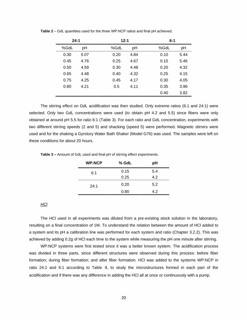
The stirring effect on GdL acidification was then studied. Only extreme ratios (6:1 and 24:1) were

selected. Only two GdL concentrations were used (to obtain pH 4.2 and 5.5) since fibers were only

obtained at around pH 5.5 for ratio 6:1 (Table 3). For each ratio and GdL concentration, experiments with

two different stirring speeds (2 and 5) and shacking (speed 5) were performed. Magnetic stirrers were

used and for the shaking a Gyrotory Water Bath Shaker (Model G76) was used. The samples were left on

these conditions for about 20 hours.

Table 3 – Amount of GdL used and final pH of stirring effect experiments.

WP:NCP % GdL pH

6:1 0.15 5.4

0.25 4.2

24:1 0.20 5.2

0.80 4.2

HCl

The HCl used in all experiments was diluted from a pre-existing stock solution in the laboratory,

resulting on a final concentration of 1M. To understand the relation between the amount of HCl added to

a system and its pH a calibration line was performed for each system and ratio (Chapter 3.2.2). This was

achieved by adding 0.2g of HCl each time to the system while measuring the pH one minute after stirring.

WP:NCP systems were first tested since it was a better known system. The acidification process

was divided in three parts, since different structures were observed during this process: before fiber

formation; during fiber formation; and after fiber formation. HCl was added to the systems WP:NCP in

ratio 24:1 and 6:1 according to Table 4, to study the microstructures formed in each part of the

acidification and if there was any difference in adding the HCl all at once or continuously with a pump.

21

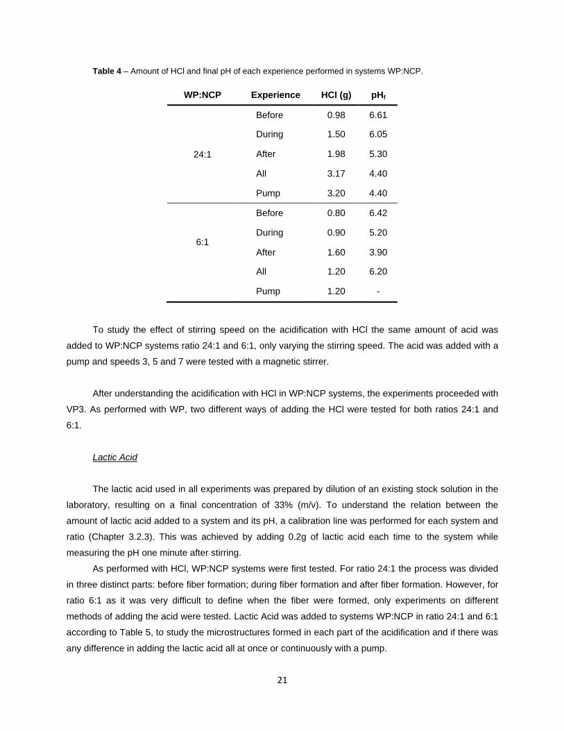
Table 4 – Amount of HCl and final pH of each experience performed in systems WP:NCP.

WP:NCP Experience HCl (g) pHf

24:1

Before 0.98 6.61

During 1.50 6.05

After 1.98 5.30

All 3.17 4.40

Pump 3.20 4.40

6:1

Before 0.80 6.42

During 0.90 5.20

After 1.60 3.90

All 1.20 6.20

Pump 1.20 -

To study the effect of stirring speed on the acidification with HCl the same amount of acid was

added to WP:NCP systems ratio 24:1 and 6:1, only varying the stirring speed. The acid was added with a

pump and speeds 3, 5 and 7 were tested with a magnetic stirrer.

After understanding the acidification with HCl in WP:NCP systems, the experiments proceeded with

VP3. As performed with WP, two different ways of adding the HCl were tested for both ratios 24:1 and

6:1.

Lactic Acid

The lactic acid used in all experiments was prepared by dilution of an existing stock solution in the

laboratory, resulting on a final concentration of 33% (m/v). To understand the relation between the

amount of lactic acid added to a system and its pH, a calibration line was performed for each system and

ratio (Chapter 3.2.3). This was achieved by adding 0.2g of lactic acid each time to the system while

measuring the pH one minute after stirring.

As performed with HCl, WP:NCP systems were first tested. For ratio 24:1 the process was divided

in three distinct parts: before fiber formation; during fiber formation and after fiber formation. However, for

ratio 6:1 as it was very difficult to define when the fiber were formed, only experiments on different

methods of adding the acid were tested. Lactic Acid was added to systems WP:NCP in ratio 24:1 and 6:1

according to Table 5, to study the microstructures formed in each part of the acidification and if there was

any difference in adding the lactic acid all at once or continuously with a pump.

22

Table 5 – Amount of lactic acid and final pH (pHf) of each experience performed in systems WP:NCP.

WP:NCP Experience Lactic

Acid (g) pHf

24:1

Before 1.60 6.32

During 2.20 5.93

After 2.60 4.73

All 1.98 3.90

Pump 2.00 4.03

6:1 All 1.60 3.50

Pump 1.60 3.60

For VP3:NCP systems, the two different ways of adding the lactic acid were experimented for both

ratio 24:1 and 6:1.

Influence of pH on the amount of protein inside the fibers

It was also tested the influence of the acidification pH on the amount of proteins retained by the

fibers, using the Bicinchoninic Acid Analysis (BCA). Systems with WP:NCP in ratios 24:1 and 6:1 were

tested at acidification pH of 4.2 and 4.8. The systems were acidified with HCl by a pump and then

centrifuged. The liquid phase was analyzed following the BCA protocol (Appendix 6.4). Yield of wet fibers

was also calculated.

2.4 Cross-linking

To improve the fiber formation all the systems and experiments was performed with a mechanical

stirrer. The systems used were VP3:NCP in ratio 6:1. The acidification method used was continuously

with a pump. Samples with both acids were tested: 2.8g to acidify with HCl; 2.2g to acidify with lactic acid.

In order to understand if cross-linking on VP3:NCP systems was possible, the first cross-linker

used was glutaraldehyde. Systems with VP3 were prepared and acidified. 5g of glutaraldehyde (1% w/w)

was added to the fibers while stirring. The system remained stirring for 10 minutes.

Experiments with two different FGC were performed using only HCl to acidify the VP3:NCP

systems. First it was tested FGC1. A system with VP3 was prepared and acidified. Then 12.5g of FGC1

(10% w/w) was added while stirring. The system remained stirring for 1 hour. FGC2 was also tested. After

consulting the producer about the safe amount of FGC allowed on food, the concentration added to the

systems was changed to 0.5% (w/w). A system with VP3 was prepared and acidified. 0.6g of FGC2 (0.5%

w/w) was added to it while stirring. The system remained stirring for 1 hour.

23

Another type of cross-linking explored was heat, a physical cross-linker. For this systems with VP3

were prepared and acidified. Samples were heated for 30 minutes in a water bath at 80ºC.

To finalize this set of experiments, the combination of the chemical cross-linker with the physical

one was performed. For all glutaraldehyde, FGC1 and 2, the experiments were performed as described

before. Before centrifuge, the fibers were heated for 30 minutes in a water bath at 80ºC.

All samples were then centrifuged for 5 minutes at 4000 G, fibers were collected, stored at 5ºC

overnight and analyzed using the CLSM. Yield of wet fibers was determined in all samples (except FGC1)

In order to determine the amount of protein retained by the fibers, Kjeldahl analysis was performed to the

fibers of all the samples, except for the ones with FGC1.

2.5 Neutralization

The NaOH used was diluted from a pre-existing stock solution in the laboratory, resulting on a final

concentration of 2M. The systems were stirred using a mechanic stirrer.

The first attempt to reach pH 7 was achieved by adding the same equivalents of NaOH as added of

HCl. The systems used were VP3:NCP in ratio 6:1. The acidification method selected was continuously

with a pump and only HCl was used (2.8g). A control sample was always performed with no cross-linking

process. The other samples were cross-linked as described before with glutaraldehyde, FGC1 and 2,

heat, FGC1 plus heat, and FCG2 plus heat. In order to increase the pH up to 7, 2.5g of NaOH was added

through a pump (100 µL/min) while the system was stirred. Although the systems were very

heterogeneous final pH of each sample was measured. Yield of wet fibers was determined in all samples.

With the purpose of better understand the relation between the amount of NaOH added to the

system and its pH, a range of different NaOH amounts was tested. Again, VP3:NCP systems were

prepared in ratio 6:1 and acidified with 2.8g of HCl through a pump (200 µL/min). The following amounts

of NaOH were tested: 0.5g; 1.0g; 1.2g; 1.5g; 2.0g; and 2.5g. The NaOH was added with a pump

(100 µL/min). Samples were left stirring overnight at room temperature, in order to reach equilibrium.

Samples were then visually analyzed.

Kjeldahl was performed to the fibers cross-linked with glutaraldehyde, FGC2, and heating, and

neutralized with the selected amount of NaOH. The analysis was performed to determine the amount of

protein retained inside the fibers.

24

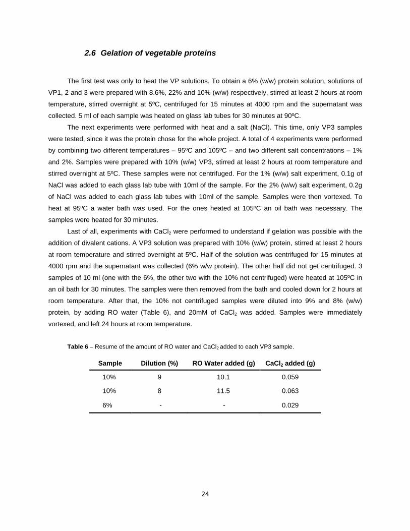
2.6 Gelation of vegetable proteins

The first test was only to heat the VP solutions. To obtain a 6% (w/w) protein solution, solutions of

VP1, 2 and 3 were prepared with 8.6%, 22% and 10% (w/w) respectively, stirred at least 2 hours at room

temperature, stirred overnight at 5ºC, centrifuged for 15 minutes at 4000 rpm and the supernatant was

collected. 5 ml of each sample was heated on glass lab tubes for 30 minutes at 90ºC.

The next experiments were performed with heat and a salt (NaCl). This time, only VP3 samples

were tested, since it was the protein chose for the whole project. A total of 4 experiments were performed

by combining two different temperatures – 95ºC and 105ºC – and two different salt concentrations – 1%

and 2%. Samples were prepared with 10% (w/w) VP3, stirred at least 2 hours at room temperature and

stirred overnight at 5ºC. These samples were not centrifuged. For the 1% (w/w) salt experiment, 0.1g of

NaCl was added to each glass lab tube with 10ml of the sample. For the 2% (w/w) salt experiment, 0.2g

of NaCl was added to each glass lab tubes with 10ml of the sample. Samples were then vortexed. To

heat at 95ºC a water bath was used. For the ones heated at 105ºC an oil bath was necessary. The

samples were heated for 30 minutes.

Last of all, experiments with CaCl2 were performed to understand if gelation was possible with the

addition of divalent cations. A VP3 solution was prepared with 10% (w/w) protein, stirred at least 2 hours

at room temperature and stirred overnight at 5ºC. Half of the solution was centrifuged for 15 minutes at

4000 rpm and the supernatant was collected (6% w/w protein). The other half did not get centrifuged. 3

samples of 10 ml (one with the 6%, the other two with the 10% not centrifuged) were heated at 105ºC in

an oil bath for 30 minutes. The samples were then removed from the bath and cooled down for 2 hours at

room temperature. After that, the 10% not centrifuged samples were diluted into 9% and 8% (w/w)

protein, by adding RO water (Table 6), and 20mM of CaCl2 was added. Samples were immediately

vortexed, and left 24 hours at room temperature.

Table 6 – Resume of the amount of RO water and CaCl2 added to each VP3 sample.

Sample Dilution (%) RO Water added (g) CaCl2 added (g)

10% 9 10.1 0.059

10% 8 11.5 0.063

6% - - 0.029

25

2.7 Addition of sunflower oil

In order to see the behavior of oil droplets on the fiber formation, experiments with sunflower oil

were performed. VP3 stock solution was prepared. An emulsion was made with 5% and 10% of sunflower

oil and the VP3 solution. Two systems were then prepared, as normal, with these two VP3/oil solutions

and acidify with 2.8g of HCl through a pump. The systems were stirred using a mechanic stirrer. Yield of

wet fibers was determined.

2.8 Large Scale

Two cross-linking methods were selected to be tested in large scale: heating at 80ºC for 30

minutes; adding 0.5% of FGC2 and stirring for 1 hour.

Four samples of 125g VP3:NCP system were prepared as normal for the FGC2 cross-linking

experiment. To shape the fibers, a 10% (w/w) egg white protein solution was mixed with the fibers on a

petri dish (20% (w/w) of protein solution). The mixed sample was heated for 30 minutes at 95ºC. After

that, the shaped product was fried in a pan following a protocol. The result was tested by three persons,

in order to evaluate its texture.

For the heat cross-linking, six samples of 125g VP3:NCP system were prepared as normal. The

fibers were then compressed to remove the excess of water. To shape the fibers, a 10% (w/w) egg white

protein solution was mixed with the fibers on a petri dish (10% (w/w) of protein solution). The mixed

sample was heated for 30 minutes at 95ºC. After that, the shaped product was fried in a pan following a

protocol. The result was tested by six persons, in order to evaluate its texture.

26

27

3 Results and Discussion

The microstructure of food products is an important aspect when trying to mimic an existing

product. The more similar the microstructures are, more similar will be the texture of the final product. To

obtain a good bite experience, the meat alternative has to have good water-retaining fibers. The

microstructures formed by coacervation of vegetable proteins and polysaccharides depend not only on

the amount of proteins dissolved on the system but also on the electric charge of the protein during

coacervation. Therefore it is important to characterize the proteins used on this project in terms of

solubility and zeta potential as function of pH. Also the influence of the type of acid and stirring speed

used to acidify was studied, as well as the best cross-linker to stabilize the fibers.

As the final meat alternative was supposed to be fibers involved on a protein matrix, experiments

with different gelation methods were tested. Additional experiments with sunflower oil were performed to

improve the taste. In the end, large scale experiments were tested in order to obtain a cooked

hamburger-type product.

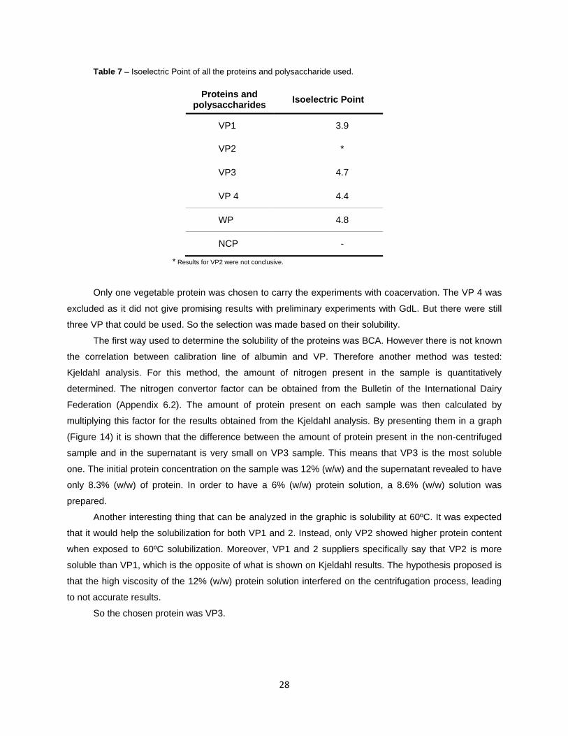
3.1 Characterization of the proteins

All proteins as well as NCP were analyzed in the Zetasizer Nano, in order to find the pI – the pH at

which the zeta potential is zero. The graphics obtained by the Zetasizer Nano are presented on Appendix

6.1. From these graphics the pI for each protein was determined (Table 7) and they are in agreement with

the literature: for acidic polypeptides the range of pI is 4.5 - 5.8 [O'Kane, 2004]. As expected NCP

remained negatively charged through the whole range of pH chosen. Therefore it has no pI. The results of

VP2 were not conclusive. This protein was tested twice and for the two times it presented different and

non-possible results. As explained before, the proteins must be positively charged in order to

coacervation happens. So the pH of acidification has to be below the pI of the proteins. Given this

panorama and in order to assure that for all proteins coacervation occurs, the pH of acidification selected

was 3.5.

28

Table 7 – Isoelectric Point of all the proteins and polysaccharide used.

Proteins and polysaccharides

Isoelectric Point

VP1 3.9

VP2 *

VP3 4.7

VP 4 4.4

WP 4.8

NCP -

* Results for VP2 were not conclusive.

Only one vegetable protein was chosen to carry the experiments with coacervation. The VP 4 was

excluded as it did not give promising results with preliminary experiments with GdL. But there were still

three VP that could be used. So the selection was made based on their solubility.

The first way used to determine the solubility of the proteins was BCA. However there is not known

the correlation between calibration line of albumin and VP. Therefore another method was tested:

Kjeldahl analysis. For this method, the amount of nitrogen present in the sample is quantitatively

determined. The nitrogen convertor factor can be obtained from the Bulletin of the International Dairy

Federation (Appendix 6.2). The amount of protein present on each sample was then calculated by

multiplying this factor for the results obtained from the Kjeldahl analysis. By presenting them in a graph

(Figure 14) it is shown that the difference between the amount of protein present in the non-centrifuged

sample and in the supernatant is very small on VP3 sample. This means that VP3 is the most soluble

one. The initial protein concentration on the sample was 12% (w/w) and the supernatant revealed to have

only 8.3% (w/w) of protein. In order to have a 6% (w/w) protein solution, a 8.6% (w/w) solution was

prepared.

Another interesting thing that can be analyzed in the graphic is solubility at 60ºC. It was expected

that it would help the solubilization for both VP1 and 2. Instead, only VP2 showed higher protein content

when exposed to 60ºC solubilization. Moreover, VP1 and 2 suppliers specifically say that VP2 is more

soluble than VP1, which is the opposite of what is shown on Kjeldahl results. The hypothesis proposed is

that the high viscosity of the 12% (w/w) protein solution interfered on the centrifugation process, leading

to not accurate results.

So the chosen protein was VP3.

29

Figure 14 - Graph of the amount of vegetable protein present on each sample tested in Kjeldahl analysis.

3.2 Acidification

Several methods of acidification were tested in protein:NCP systems: slow acidification;

acidification with a strong acid; acidification with a weak acid; batch acidification; and continuous

acidification. Acidifying continuously with a strong acid turned out to give the best fibers.

3.2.1 GdL

Optimization of GdL amount

The objective of determining the optimum amount of GdL to achieve the desired pH of 4.2 was

achieved (Table 8) and can be seen on detail on Appendix 6.3. However the results of slow acidification

with GdL experiments without stirring were not the ones expected. Fibers were only formed for system

WP:NCP ratio 6:1. Surprisingly, this was obtained when the final pH was 5.5 (0.15% w/w of GdL).

According to the pI of WP (4.8), at this pH the protein is still negative. For the other systems ratio only a

hard gel network was observed. The gel was always white and its consistency changed depending on the

system ratio (24:1 ratio gel was the hardest of all). When pressed it broke very easily and a lot of water

was released (Figure 15).

0.0

2.0

4.0

6.0

8.0

10.0

VP 1 VP 2 VP 3

Pro

tein

co

nte

nt

(%

w/w

)

Non-Centrifuged

Supernatant

Supernatant 60°C

30

Table 8 – Resume of the results concerning the optimum amount of GdL to achieve pH 4.2 in WP:NCP systems.

WP:NCP ratio Optimal GdL amount (% w/w)

24:1 0.80

12:1 0.45

6:1 0.24

Figure 15 – Example of WP:NCP systems after acidification with GdL: white watery gel.

Looking into the gel microstructure (an example is presented on Figure 16), in the majority of the

samples no fiber structure was formed. Instead, the gel was composed of a very heterogeneous network

of proteins. The higher the GdL concentration was, the stiffest the gel become. On system WP:NCP ratio

6:1 with 0.15% (w/w) of GdL, some fiber structures were found and its microstructure was analyzed with

CLSM (Figure 17). Unlike the gel, in these structures proteins are all aligned forming fibers. However, the

results were not satisfactory since the fibers represented only a very small part of the sample.

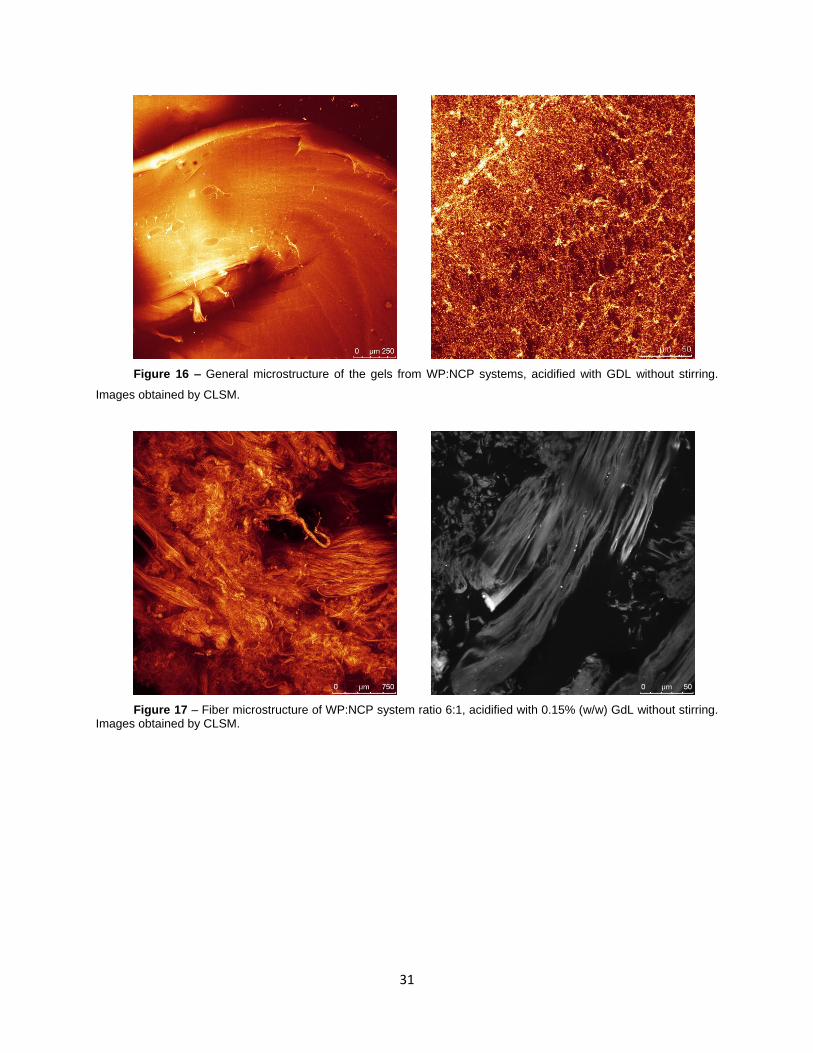
31

Figure 16 – General microstructure of the gels from WP:NCP systems, acidified with GDL without stirring.

Images obtained by CLSM.

Figure 17 – Fiber microstructure of WP:NCP system ratio 6:1, acidified with 0.15% (w/w) GdL without stirring. Images obtained by CLSM.

32

Stirring effect

The stirring impact on the fiber formation was then analyzed. For that, a control without stirring was

always preformed and only ratio 24:1 and 6:1 were tested, since they represented the two extremes. Also

two concentrations of GdL were tested for each ratio in order to achieve pH 4.2 and 5.5.

Results showed that for WP:NCP ratio 24:1 at pH 5.2 the systems remains a very viscous

translucent liquid, even with different stirring speeds (Figure 18 A). On the other hand at pH 4.5 the

control sample becomes a hard gel as shown before (Figure 18 B). If the sample is slowly stirred at

speed 2 (maximum speed 10, correspondent to 1100 rpm) the system is completely different from the

control and some sort of fibers were formed (Figure 19). But if the speed is increased up to 5, the system

remains liquid and no fiber is formed (Figure 20). The same happens when the sample is shacked at

speed 5.

Figure 18 - Systems WP:NCP ratio 24:1, without stirring: A) pH 5.2, B) pH 4.2. Images obtained by CLSM.

A) B)

33

Figure 19 - System WP:NCP ratio 24:1, with slow stirring (speed 2) at pH 5.2. Images obtained by CLSM.

Figure 20 - System WP:NCP ratio 24:1, with slow stirring (speed 5) at pH 5.2. Images obtained by CLSM.

For the system WP:NCP ratio 6:1 there were already fibers on the control sample at pH 5.2 (Figure

17). When the system was acidified under stirring conditions (speed 2 or 5), a hard gel was formed, and

the only difference between speeds was that in speed 5 the system was composed by a liquid part and a

solid gel. The shaken experiment at speed 5 resulted on an heterogeneous agglomerated of proteins and

sort of fibers (Figure 21 A). For the system WP:NCP ratio 6:1 at pH 4.2, the results were all the same for

every experiment: a hard gel was formed. Even though different structures were found when changing the

speed, there was no fiber formation.

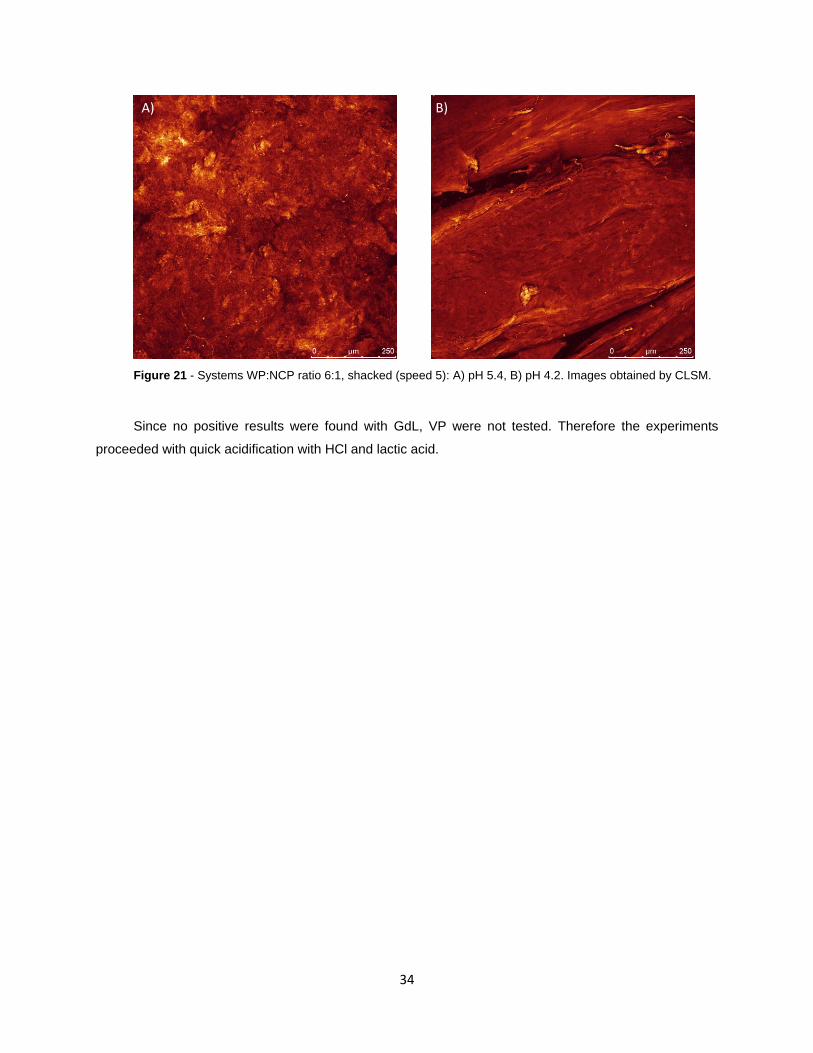
34

Figure 21 - Systems WP:NCP ratio 6:1, shacked (speed 5): A) pH 5.4, B) pH 4.2. Images obtained by CLSM.

Since no positive results were found with GdL, VP were not tested. Therefore the experiments

proceeded with quick acidification with HCl and lactic acid.

A) B)

35

3.2.2 HCl

To understand the relation between the amount of HCl added to the systems and its pH, a

calibration line was performed for 125g of each system and ratio (Figure 22 and 23). The pH measuring

was not always easy, since fibers were forming and the pH was very unstable within the heterogeneous

system. For systems with ratio 24:1 either with WP or VP3, the pH was more stable, which affected the

smoothness of the curve (Figure 22 and 23). The opposite was observed when adding HCl to 6:1 ratio

systems, especially for VP3. It seemed like the system started by acting like a buffer, not lowering the pH

while HCl was added. And in one point, one acid drop was added and the pH just completely changed

into a low pH, and then fibers appeared.

The amounts of HCl selected to acidify each system are resumed on Table 9.

Table 9 – Resume of the amounts of HCl necessary to achieve pH 3.5 on the different systems tested.

System Ratio HCl (g)

WP:NCP 24:1 3.2

6:1 1.2

VP3:NCP 24:1 8.6

6:1 2.8

Figure 22 – Graphics of the amount of acid added versus the pH of the system WP:NCP ratio 24:1 and 6:1.

3.50

4.50

5.50

6.50

7.50

0.0 1.0 2.0 3.0

pH

HCl amount (g)

WP:NCP 24:1 Adition of HCl 1M

3.50

4.50

5.50

6.50

7.50

0.0 1.0 2.0 3.0

pH

HCl amount (g)

WP:NCP 6:1 Adition of HCl 1M

36

Figure 23 – Graphic of the amount of acid added versus the pH of the system VP3:NCP ratio 24:1 and 6:1.

WP

While making the calibration line with HCl it was evident that, based on visual observation, the

acidification could be divided in three phases. First it started by forming translucent pearls each time the

acid was added. It seemed that, in the moment that the acid was added, coacervation happened locally

forming a pearl and trapping the remaining acid inside it. The more acid was added, the more pearls were

formed. Then, at one point, the solution is completely full of elongated pearls (due to stirring) and a few

fibers, and by adding just a drop of acid the whole pearls turn into white thick fibers. After this the acid

added contributed directly to lowering the pH. These three parts were named as “before”, “during” and

“after” fiber formation (Figure 24). If the pearls are left for some time, they become white as in Figure 24

A).

Figure 24 – Three different phases of fiber formation on systems WP:NCP ratio 24:1: Before (A); During (B); and After (C) fiber formation.

3.00

4.00

5.00

6.00

7.00

8.00

0.0 2.0 4.0 6.0 8.0

pH

HCl amount (g)

VP3:NCP 24:1 Adition of HCl 1M

3.00

4.00

5.00

6.00

7.00

8.00

0.0 2.0 4.0 6.0 8.0

pH

HCl amount (g)

VP3:NCP 6:1 Adition of HCl 1M

A) B) C)

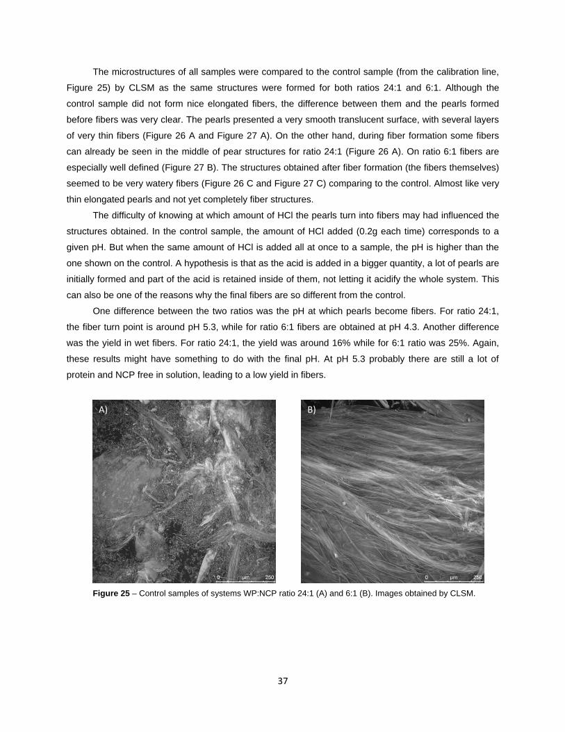
37

The microstructures of all samples were compared to the control sample (from the calibration line,

Figure 25) by CLSM as the same structures were formed for both ratios 24:1 and 6:1. Although the

control sample did not form nice elongated fibers, the difference between them and the pearls formed

before fibers was very clear. The pearls presented a very smooth translucent surface, with several layers

of very thin fibers (Figure 26 A and Figure 27 A). On the other hand, during fiber formation some fibers

can already be seen in the middle of pear structures for ratio 24:1 (Figure 26 A). On ratio 6:1 fibers are

especially well defined (Figure 27 B). The structures obtained after fiber formation (the fibers themselves)

seemed to be very watery fibers (Figure 26 C and Figure 27 C) comparing to the control. Almost like very

thin elongated pearls and not yet completely fiber structures.

The difficulty of knowing at which amount of HCl the pearls turn into fibers may had influenced the

structures obtained. In the control sample, the amount of HCl added (0.2g each time) corresponds to a

given pH. But when the same amount of HCl is added all at once to a sample, the pH is higher than the

one shown on the control. A hypothesis is that as the acid is added in a bigger quantity, a lot of pearls are

initially formed and part of the acid is retained inside of them, not letting it acidify the whole system. This

can also be one of the reasons why the final fibers are so different from the control.

One difference between the two ratios was the pH at which pearls become fibers. For ratio 24:1,

the fiber turn point is around pH 5.3, while for ratio 6:1 fibers are obtained at pH 4.3. Another difference

was the yield in wet fibers. For ratio 24:1, the yield was around 16% while for 6:1 ratio was 25%. Again,

these results might have something to do with the final pH. At pH 5.3 probably there are still a lot of

protein and NCP free in solution, leading to a low yield in fibers.

Figure 25 – Control samples of systems WP:NCP ratio 24:1 (A) and 6:1 (B). Images obtained by CLSM.

A) B)

38

Figure 26 – Different structures obtained during the three phases of acidification in WP:NCP system ratio 24:1: before (A), during (B) and after (C) fiber formation. Images obtained by CLSM.

A) B)

C)

39

Figure 27 - Different structures obtained during the three phases of acidification in WP:NCP system ratio 6:1:before (A), during (B) and after (C) fiber formation. Images obtained by CLSM.

A) B)

C) C)

40

Experiments were performed in order to understand the differences of adding HCl all at once or

slowly with a pump, as some differences were found when adding the acid in different ways.

When looking to the final fibers of ratio 24:1 (Figure 28), there are no big differences between

adding the acid all at once or through a pump. Comparing them at the microscopic level (Figure 29), all

the fibers appear to be very organized and aligned. These results are very different from the ones

obtained for the control sample (Figure 25 A), where only a few fibers can be observed.

Figure 28 – WP:NCP ratio 24:1 fibers, obtained by adding HCl all at once (A) and with a pump (B).

Figure 29 - Fiber microstructures obtained with the addition of HCl in WP:NCP system ratio 24:1 all at once (A) and with a pump at the rate 200 μL/min (B). Images obtained by CLSM.

A) B)

A) B)

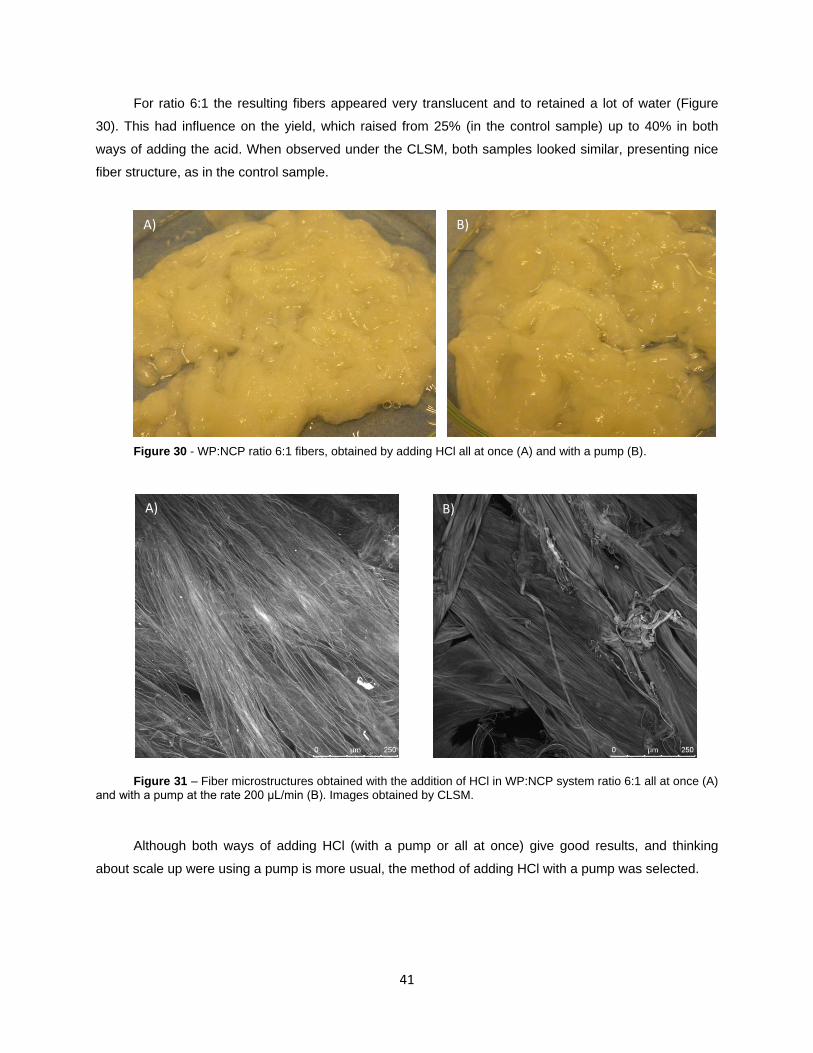
41

For ratio 6:1 the resulting fibers appeared very translucent and to retained a lot of water (Figure

30). This had influence on the yield, which raised from 25% (in the control sample) up to 40% in both

ways of adding the acid. When observed under the CLSM, both samples looked similar, presenting nice

fiber structure, as in the control sample.

Figure 30 - WP:NCP ratio 6:1 fibers, obtained by adding HCl all at once (A) and with a pump (B).

Figure 31 – Fiber microstructures obtained with the addition of HCl in WP:NCP system ratio 6:1 all at once (A) and with a pump at the rate 200 μL/min (B). Images obtained by CLSM.

Although both ways of adding HCl (with a pump or all at once) give good results, and thinking

about scale up were using a pump is more usual, the method of adding HCl with a pump was selected.

B) A)

A) B)

42

To understand the influence of the stirring speed on the quality of the fibers, experiments with the

same pump rate and different stirring speeds were performed. To compare, a control sample was

prepared adding 0.2g of HCl each time, just like with the calibration line (Figure 22).

The first ratio to be tested was 24:1. Looking at the microstructures formed (Figure 32) if the stirring

speed is too low (B) a few fibers appear, giving place pearl structures. These are easily seen on the

CLSM since they have only very thin layers of translucent fibers, and a lot of emptiness between them.

Also when stirring at speed 3 the pH remains at the initial value (Table 10). The explanation can be that

as the stirring is so slow, the acid does not have time to mix in the whole system. Therefore local

coacervation happens, giving form to the pearls shape structures. These pearls trap the remaining acid

inside, not letting coacervation happen to the remaining solution, not lowering the pH.

Figure 32 – Fiber microstructures of systems WP:NCP ratio 24:1 in different stirring speeds: Control (A), Speed 3 (B), Speed 5 (C), Speed 7 (D). Images obtained by CLSM.

A) B)

C) D)

43

At speed 5 (Figure 32 C) the system has already some fibers but it is visible still some smooth

lumps (pearls). The best fibers are obtained at speed 7 (Figure 32 D). However, they appeared to be

extremely dry, and that was also revealed in the wet fiber yield (only 11%).

Table 10 – Final pH and yield on wet fibers of WP:NCP samples.

WP:NCP Speed pHf Yield (%)

24:1

Control 4.9 24

3 6.8 29

5 4.8 22

7 4.9 11

6:1

Control 3.7 28

3 6.9 26

5 4.7 36

7 3.8 78

For ratio 6:1 (Figure 33) with stirring speed 3 (B) the fibers obtained were very watery. When

compressed they released a lot of water. However, at the microscopic level it is visible that there are well

defined fibers. Some smooth structures are also visible, corresponding to some pearl structures still

present on the sample. As explained before, these pearl structures may be the cause of the high pH on

the sample (Table 10).

If the speed is increase to 5 (C) the same lumps from ratio 24:1 appears. When the acid is added

at high speed 7 (D) the fibers formed retain a lot of water (yield in wet fibers of almost 80%). However

they lose water constantly, and after a week they were still losing it (around 2.5g water per day).

In conclusion, with a low initial yield we obtain stable fibers with no water loss. If the initial yield is

high, the final fibers will be unstable and will lose water over time.

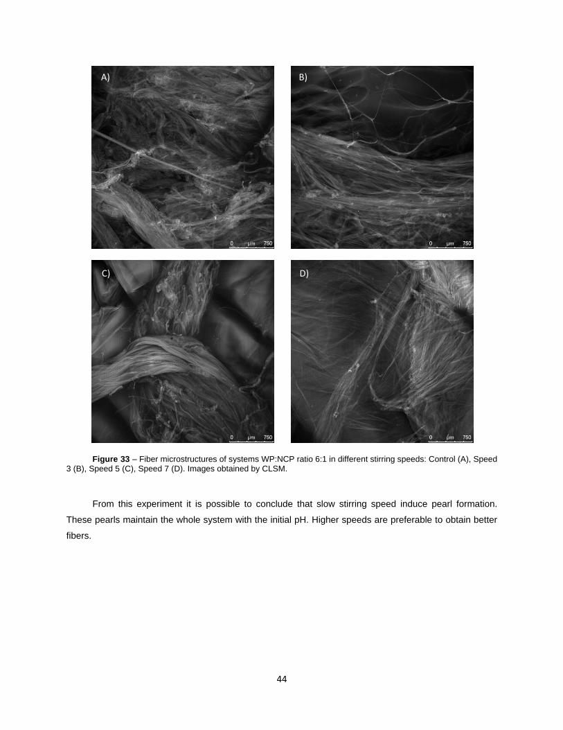
44

Figure 33 – Fiber microstructures of systems WP:NCP ratio 6:1 in different stirring speeds: Control (A), Speed 3 (B), Speed 5 (C), Speed 7 (D). Images obtained by CLSM.

From this experiment it is possible to conclude that slow stirring speed induce pearl formation.

These pearls maintain the whole system with the initial pH. Higher speeds are preferable to obtain better

fibers.

A) B)

C) D)

45

Vegetable protein

Having all the data from systems WP:NCP, experiments with VP were then study. The two already

studied methods of adding HCl were tested in VP3:NCP systems: all at once and with a pump. For each

ratio, a control sample by adding 0.2g at each time was performed.

Looking at both control samples (Figure 34), a great difference in the amount of water content was

observed. With ratio 24:1, a paste similar to dough was formed. On the other hand, with ratio 6:1 there

were evident fiber structures. When observed under the CLSM (Figure 35), in control sample for ratio

24:1 there were no fibers, and for 6:1 ratio the fibers were very watery as expected.

Figure 34 – Control samples: fibers obtained with HCl and VP3:NCP systems ratio 24:1 (A) and 6:1 (B).

Figure 35 – Fiber microstructures on control samples with VP3:NCP systems ratio 24:1 (A) and 6:1 (B). Images obtained by CLSM.

A) B)

A) B)

46

When the acid is added all at once, for ratio 24:1 it appears that fibers are formed (Figure 36 A).

However, looking in a microscope scale, no fibers were found. This can be explained with the

Voorn-Overbeek theory: above the critical polymer concentration, self-suppression of the coacervation

occurs [Overbeek and Voorn, 1957]. When one of the polymers is in excess, coacervation does not occur

because of the low energetic interest of concentrating the polymers in one phase if the concentration is

already high. The hypothesis is that VP3 is in excess on systems with 24:1 ratio.

With ratio 6:1 the final fibers were very watery as shown on Figure 36 B. And in the CLSM good

retaining fibers were visualized.

If the acid is added with a pump, ratio 24:1 remains the same, without fibers. But for ratio 6:1, the

pump improved the fibers quality (Figure 38).

Figure 36 - VP3:NCP ratio 24:1 (A) and 6:1 (B) fibers, obtained by adding HCl all at once.

Figure 37 - Fiber microstructures obtained by adding HCl all at once on samples with VP3:NCP systems ratio 24:1 (A) and 6:1 (B). Images obtained by CLSM.

A) B)

A) B)

47

Figure 38 - Fiber microstructures obtained by adding HCl with a pump on samples with VP3:NCP systems ratio 24:1 (A) and 6:1 (B). Images obtained by CLSM.

For all samples, the remaining liquid phase still contain proteins since it was very turbid.

In conclusion, for VP3:NCP systems, the best ratio is 6:1 and good fibers are obtained either by

adding HCl all at once or with a pump. However, due to the reasons given before with WP, the method of

adding with a pump was selected.

A) B)

48

3.2.3 Lactic acid

After understanding the acidification with a strong acid, a weak acid – lactic acid – was tested. As

performed with HCl, a calibration line was obtained for 125g of each system and ratio (Figure 39 and 40).

The pH measuring was even harder compared to HCl. The pH was very unstable and for all systems

seemed like the system was acting like a buffer, not lowering the pH while the acid was added. On a

certain point, one acid drop was added and the pH just dropped into unwanted values, as it visible on the

calibration graphics.

The amounts of lactic acid selected to acidify each system to pH 3.5 are resumed on Table 11.

Table 11 - Resume of the amounts of lactic acid necessary to achieve pH 3.5 on the different systems tested

System Ratio Lactic acid (g)

WP:NCP 24:1 2.0

6:1 1.6

VP3:NCP 24:1 4.8

6:1 2.2

Figure 39 – Graphic of the amount of acid added versus the pH of the system WP:NCP ratio 24:1 and 6:1.

4.00

5.00

6.00

7.00

0.0 0.5 1.0 1.5 2.0

pH

Lactic Acid amount (g)

WP:NCP 24:1 Adition of Lactic Acid 33%

3.00

4.00

5.00

6.00

7.00

0.0 0.5 1.0 1.5

pH

Lactic Acid amount (g)

WP:NCP 6:1 Adition of Lactic Acid 33%

49

Figure 40 – Graphic of the amount of acid added versus the pH of the system VP3:NCP ratio 24:1 and 6:1.

WP

Once again, while making the calibration line with lactic acid, the acidification could be divided in

three phases: before, during and after fiber formation. Experiments to visualize each part was performed.

However, as the structures formed were exactly the same as the ones formed with HCl, the images are

not presented. The abundance of pearl structures after the fiber formation with lactic acid was the main

difference between the two acids.

The results obtained for lactic acid acidification were very similar to the ones obtained with HCl. For

WP:NCP systems ratio 24:1 nice fibers were formed on the control sample (Figure 41). When the acid

was added all at once the fibers became very dry (Figure 42 A). On the other hand, when the pump was

used to add the acid a few pearls were still formed along with the fibers (Figure 42 B).

Figure 41 - Control sample of system WP:NCP ratio 24:1 after lactic acid acidification. Image obtained by CLSM.

3.00

4.00

5.00

6.00

7.00

8.00

0.0 2.0 4.0

pH

Lactic Acid amount (g)

VP3:NCP 24:1 Adition of Lactic Acid 33%

3.00

4.00

5.00

6.00

7.00

8.00

0.0 1.0 2.0

pH

Lactic Acid amount (g)

VP3:NCP 6:1 Adition of Lactic Acid 33%

50

Figure 42 - Fiber microstructures obtained by adding lactic acid in WP:NCP systems ratio 24:1: all at once (A) and with a pump (B). Images obtained by CLSM.

Due to a series of setbacks, for system WP:NCP ratio 6:1 only the control and the samples

acidified with a pump were performed. Although nice microstructural fibers were obtained (Figure 43), the

majority of system was composed by pearls. This made the sample resemble more a watery gel than

fibers.

Figure 43 - Fiber microstructures obtained by adding lactic acid in WP:NCP systems ratio 6:1: control (A) and with a pump (B). Images obtained by CLSM.

Since a lot of pearls are formed with lactic acid, we can conclude from these experiments that

acidification with HCl is preferable to acidification with lactic acid.

A) B)

A) B)

51

Vegetable protein

Even though lactic acid was not a good option for WP:NCP systems, experiments were performed

with VP3. The two methods of adding lactic acid were tested in VP3:NCP systems: all at once and with a

pump. As before, for each ratio a control sample by adding 0.2g at each time was performed.

Once again, the differences were visible between both ratios. Systems with ratio 24:1 did not form

any fibers, either when adding the acid all at once or with a pump. Instead, a thick paste similar to dough

was formed (Figure 44 A). The non-existence of fibers was verified when the samples were analyzed with

the CLSM (Figure 44 B).

Figure 44 – Example of the texture of the fibers obtained after VP3:NCP ratio 24:1 acidification with lactic acid (A) and its microstructure obtained by CLSM (B).

On the other hand, systems with ratio 6:1 formed well defined fibers (Figure 45 and 46). There

were no significant differences between the two methods of adding the acid. However, both fibers

appeared to be extremely dry when compared to the ones obtained with HCl.

A) B)

52

Figure 45 - Control sample of system VP3:NCP ratio 6:1 acidified with lactic acid (A) and its microstructure obtained by CLSM (B).

Figure 46 - Fiber microstructures obtained by adding lactic acid in VP3:NCP systems ratio 6:1: all at once (A) and with a pump (B). Images obtained by CLSM.

The remaining liquid phase of both ratios was less turbid than the one from acidification with HCl.

This may lead to conclude that using lactic acid avoids wasting protein in the remaining liquid phase.

However, as the fibers formed were very dry, HCl was selected also for VP3 systems as the best acidifier.

One explanation for the better results with HCl can be that as it is a smaller molecule (than the lactic acid)

it does not interfere with the structure protein-polysaccharide.

A) B)

A) B)

53

3.2.4 Influence of pH on the amount of protein inside the fibers

In order to know the yield of proteins that was retained inside the fibers, the amount of proteins

remaining on the liquid after coacervation was measured. This was done using BCA (Figure 47). Systems

with WP:NCP in ratios 24:1 and 6:1 at two different pH were tested. As pH 4.8 is the pI of WP, it was

tested with pH 4.2, which was the first selected pH for acidification. The systems were acidified using the

optimum conditions selected: adding HCl slowly through a pump. Calibration line and results of the

samples OD are presented on Appendix 6.4. Even though the samples were diluted 1:10, samples from

ratio 24:1 were still very concentrated. These two results were not covered by the calibration line.

However, as the difference was not significant and this analysis was only to get a general overview, the

results were accepted.

Figure 47 – Example of one plate of BCA ready to be analyzed

Table 12 - Protein concentration and yield in the wet fibers obtained with WP:NCP systems at different pH.

WP:NCP pH Yield

Wet mass (%) Protein Concentration in the liquid (mg/ml)

Protein Yield in the wet mass (%)

24:1 4.2 27.3 21.5 ±0.1 55

4.8 32.2 22.6 ±0.1 53

6:1 4.2 28.2 4.5 63

4.8 33.3 5.9 51

The results showed that the lower the final pH less protein remains in the liquid phase. However,

even with the lower pH there is still a lot of protein that is not retained by coacervation. Almost 50% of the

initial protein remains on the liquid phase and there are no significant differences between the two ratios.

Further experiments are required to improve this yield. Determination of NCP quantities present in the

liquid phase is important. In this way it is possible to know if the system reached and equilibrium or if it is

the protein that is in excess.

54

3.3 Cross-linking

After optimizing the parameters to obtain good water-retaining fibers, a cross-linking study was the

next step. Different chemical and physical cross linkers were tested in VP3:NCP systems ratio 6:1. All the

systems and experiments were prepared with a mechanic stirrer, since a magnet stirrer was not strong

enough to stir at high speed. To have a comparison, a control sample was always performed without any

cross-linking.

3.3.1 Glutaraldehyde

The first experiments were performed before knowing the results of which acidification was better

(with a strong or a weak acid). Therefore systems acidified with both acids were cross-linked with

glutaraldehyde.

HCl

When comparing fibers with cross-linking to without it, the darker yellow color was the main

difference (Figure 48). The cross-linked sample presented some difficulties while trying to remove the

fibers from the stirrer. The fibers were very strong. Sample without cross-linking formed also good fibers,

and both of the fibers retained some water, as the yield was around 25%.

Using the CLSM the explanation to why the cross-linked fibers were so stiff was observed.

Although the samples are not homogeneous, as generally in this project, a specific microstructure was

very present in the cross-linked sample. As visible in Figure 49 B, the sample consisted of a majority of

fibers resembling twisted ropes. This explained the extra strength between fibers when the sample is

pulled to opposite sides.

Figure 48 – Fibers obtained from VP3:NCP and HCl: control (A) and cross-linked with glutaraldehyde (B).

A) B)

55

Figure 49 - Fiber microstructures obtained in VP3:NCP systems ratio 6:1 and HCl: control (A) and cross-linked with glutaraldehyde (B). Images obtained by CLSM.

Lactic Acid

The results obtained with samples acidified with lactic acid were similar as the ones obtained with

HCl (Figure 50). Both cross-linked and non-cross-linked samples formed good fibers, with around 20%

yield in wet fibers. The cross-linked sample did not present the same stiffness than the previous one with

HCl, and that could be visualized with CLSM (Figure 51). The twisted ropes microstructures were less

common, giving place to simple normal aligned fiber like structures.

Figure 50 – Fibers obtained from VP3:NCP and lactic acid: control (A) and cross-linked with glutaraldehyde (B).

A) B)

A) B)

56

Figure 51 - Fiber microstructures obtained in VP3:NCP systems ratio 6:1 and lactic acid: control (A) and cross-linked with glutaraldehyde (B). Images obtained by CLSM.

A) B)

57

3.3.2 Food grade cross-linking agents

Two different FGC were studied. All experiments were performed in fibers obtained with HCl

acidification. The samples were compared to the control sample presented in Figure 48 A and 49 A.

Fibers cross-linked with FGC1 got an intense yellow color (Figure 52 A) as this compound is a

brown-yellow solution. The fibers formed appeared to be very watery and soft. These fibers were not as

stiff as the ones cross-linked with glutaraldehyde. When pulled to opposite sides the fibers easily

separated themselves. When compressed, a lot of water was also released. On the microscope scale, the

usual fiber structure was present (Figure 52 B). No significant difference was observed when compared to

the control sample. Yield on wet fibers was not calculated for this experiment since the samples had to be

divided (in a not precise way due to the big fiber lumps) in two to another experiment.

Figure 52 - Fibers obtained from VP3:NCP and HCl, cross-linked with FGC1 (A) and its microstructure obtained by CLSM (B).

A) B)

58

FGC2 was also a brown solution. The fibers obtained by cross-linking with FGC2 were very similar

to muscle (Figure 53). The yield on wet fibers was 21% and the fibers were again very stiff and hard to

break. When observed under the CLSM, the microstructures are very similar to meat.

Figure 53- Fibers obtained from VP3:NCP and HCl, cross-linked with FGC2 (A) and its microstructure obtained by CLSM (B).

3.3.3 Heat

Heating the fibers at 80ºC for 30 minutes was another method tested to cross-link. Fibers were

compared to the control sample already presented in Figure 48 A and 49 A. The fibers presented a good

yield (27%), meaning that heating process helps to retain water inside the fibers. The CLSM results show

good fiber microstructures (Figure 54).

Figure 54 - Fibers obtained from VP3:NCP and HCl, cross-linked by heating (A) and its microstructure obtained by CLSM (B).

A) B)

A) B)

59

3.3.4 Chemical and Heat

To finish the cross-linking experiments, a combination of both chemical and physical cross-linkers

was tested. Glutaraldehyde and FGC1 and 2 cross-linking experiments were performed as before, but

before being analyzed the samples were heated at 80ºC for 30 minutes.

Figure 55 - Fibers obtained from VP3:NCP and HCl, cross-linked with glutaraldehyde and heating (A) and its microstructure obtained by CLSM (B).

The results can be generalized to all samples. The first difference between heated and non-heated

samples was the color. Cross-linking with a chemical compound and heat made the fibers go darker. Also

the fibers become stiffer and harder to separate from the stirrer. The yield of each sample remained the

same. However, fibers looked drier than when only cross-linked with the compound. This suggests that

after cross-linked with a chemical compound the fibers do not gain more water when heated.

Looking at the results in a microstructure scale, fibers appeared to be more aggregated in twisted

rope shape. This explains the stiffness of the fibers. All of the samples resemble a lot meat fibers.

A) B)

60

Figure 56 - Fibers obtained from VP3:NCP and lactic acid, cross-linked with glutaraldehyde and heating (A) and its microstructure obtained by CLSM (B).

Figure 57 - Fibers obtained from VP3:NCP and HCl, cross-linked with FGC1 and heating (A) and its microstructure obtained by CLSM (B).

A) B)

A) B)

61

Figure 58 - Fibers obtained from VP3:NCP and HCl, cross-linked with FGC2 and heating (A) and its microstructure obtained by CLSM (B).

Although all the experiments presented good results, only cross-linking with FG2 and cross-linking

with heat alone were selected to be tested in large scale.

3.4 Neutralization

Even though good fibers were obtained with all the experiments before presented they all were

around pH 3. This pH is not suitable for meat alternatives, which have a neutral pH. For that reason the

next goal was to bring the fibers back to neutral pH (around 6 - 7).

Thinking that adding the same number of moles of NaOH and HCl was all that was necessary, the

first experiments were performed to systems cross-linked with FGC1 and 2, heat and the combination of

FGC1 and 2 with heat. Experiences with glutaraldehyde were only performed to determine the yield and

amount of protein retained inside the fibers.

Getting the fibers to neutral pH turned out to be more difficult than expected. As the system was

composed of a liquid phase and a lump of fibers, mixing the NaOH in a homogeneous way was hard. The

NaOH was added 0.2g each time. As more NaOH was being added, the systems become with the liquid

phase more turbid and with the fiber lump more compact. The pH measured on the liquid phase did not

correspond to the pH measured if the electrode was in the middle of the fibers. Usually in the fibers the

pH was lower. So while the pH on the liquid was already 10, in the fibers was still 4. As the pH on the

liquid was going higher, the fibers started to dissociate and the reverse process of coacervation

happened. The graphic in Figure 59 resumes the yields in wet fibers obtained. As explained before, for

cross-linking with FGC1 the yield was not accurately calculated, so the results are not presented. As

coacervation is reversible, it was expected that after neutralization there would be no fibers present,

which was verified. Glutaraldehyde was the cross-linker that better worked in protecting the fibers during

A) B)

62

the neutralization, as no fiber was lost. The protection effect also worked with the other cross-linkers,

even though the yield was reduced.

Figure 59 - Differences on the yield in wet fibers of VP3:NCP ratio 6:1 before and after neutralization.

To determine the yield also in terms of the amount of protein retained inside the fibers and their

water holding capacity, Kjeldahl analysis was performed: Samples cross-linked with glutaraldehyde,

FGC2 and heat, as well as the control sample were analyzed before and after neutralization. The results

(Figure 60 and 61) show that most of the protein is retained in the fibers for all the cross-linking

processes. After the neutralization, fibers cross-linked with both FGC2 and heat still had a good amount

of protein present, around 60%. As expected there was no loss of protein with glutaraldehyde. These

results indicate that cross-linking is efficient on protecting also the proteins inside the fibers.

The results on the water holding capacity reveal that the FGC induces water retaining at low pH.

Figure 60 – Graphic of the protein yield in fibers of VP3:NCP ratio 6:1 before and after neutralization.

0

5

10

15

20

25

30

35

Control Glutaraldehyde FGC2 Heat FGC2 and Heat

Yie

ld in

we

t fi

be

rs (

%)

Cross-linkers

Yield in wet fibers

pH 3.5

pH 7

0

20

40

60

80

100

Control Glutaraldehyde FGC2 Heat

Pro

tein

yie

ld i

n f

ibers

(%

m/m

)

Protein yield in fibers

pH 3.5

pH 7

63

Figure 61 - Graphic of the water holding capacity of fibers VP3:NCP ratio 6:1 before and after neutralization.

The aspect of the final fibers was similar in all of the samples (Figure 62). In the middle there was a

very compacted role of fibers. As we move away from the center the fibers become more and more

viscous and soft. Until the point where only exists a very thick layer of NCP mixed with proteins. When

observed at the CLSM the microstructures remained the same, with very well defined fibers.

Figure 62 – Example of fibers from VP3:NCP systems 6:1 ratio, obtained after adding NaOH.

After realizing the difficulty of bringing the fibers pH back to 7, a range of different quantities of

NaOH were tested in order to determine the optimum amount to add (Figure 63). The systems were left

stirring overnight to ensure that the systems reached equilibrium. NaOH was added very slowly, with a

pump, and six different amounts were tested in 125g of VP3:NCP systems, acidified with HCl. The results

are presented on the graph of Figure 63.

0

5

10

15

20

25

30

Control Glutaraldehyde FGC2 Heat

Wa

ter

ho

ldin

g c

ap

acit

y (

m/m

)

Water holding capacity of fibers

pH 3.5

pH 7

64

With more than 2 g of NaOH, the system just returns all into liquid state, with a pH higher than 9.8.

Also, less than 0.5g does not change the fibers or their pH (which remains at 3.6). The fibers obtained

with 1.5g were to smooth and already viscous and their pH was also a little higher than 7. So the choice

of the amount of NaOH to add was left to two quantities: 1.2 or 1 g.

Figure 63 –Graphic with results of pH versus the amount of NaOH in 125g of system with VP3:NCP ratio 6:1

With 1.2g of NaOH the pH obtained was 6.8, but the fibers were also starting to appear very

smooth comparing to the one obtained with 1g of NaOH. These last ones were still stiff. This amount was

selected as being the optimal amount of NaOH to add to 125g of fibers systems, as the pH was 5.8 (an

acceptable value).

3.00

5.00

7.00

9.00

11.00

0.0 0.5 1.0 1.5 2.0 2.5 3.0

pH

NaOH amount (g)

Adition of NaOH 2M

65

3.5 Gelation of vegetable proteins

The final objective of this project was not only to create fibers but also to give them the familiar

shape of an hamburger. One way of doing that was to involve the fibers on a protein matrix. To create the

matrix, a serial of experiments were performed with VP solution.

3.5.1 Heat

The first attempt on creating a protein matrix was just by heating the solution. All the VP1 to 3 were

tested. As normal, only the supernatant was used, and proteins were heated up to 90ºC. This

temperature was chosen since the gelation temperature of VP achieve a peak at 89ºC [Sun and Arntfield,

2011].

However the results did not turn out to be as good as expected. VP1 and 3 did not form any gel,

remaining as liquid as initially. Only VP2 became more viscous, but still no hard gel was formed.

3.5.2 Heat and salt

Adding a salt and heating the protein solution was the next experiment. This time only VP3 was

tested and the whole solution without centrifugation was used. Two different temperatures were also

tested: 95ºC and 105ºC. NaCl was used in two concentrations, 1 and 2% (w/w) for each temperature.

At 105ºC no sample formed a gel, becoming even more liquid. On the other hand, when heated

only at 95ºC, the samples became more viscous. However, neither of two salt concentrations formed a

stiff gel.

3.5.3 Heat and CaCl2

The last attempt was to get the gels using divalent ions, testing the hypothesis that divalent ions

give stronger gels than monovalent ions. CaCl2 was used according to [Maltais et al, 2005]. Again, only

VP3 solution was used. This time the supernatant was also tested. Samples were heated at 105ºC,

diluted and added CaCl2.

After 24h, the results were quite interesting. All samples precipitated. However, only the

supernatant sample formed a sort of gel. But this gel was very weak, falling apart very easily.

So in conclusion, no protein matrix was obtained with the VP and the conditions experimented.

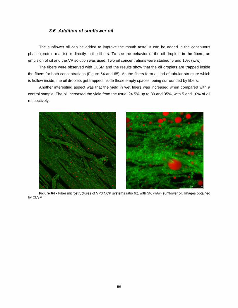
66

3.6 Addition of sunflower oil

The sunflower oil can be added to improve the mouth taste. It can be added in the continuous

phase (protein matrix) or directly in the fibers. To see the behavior of the oil droplets in the fibers, an

emulsion of oil and the VP solution was used. Two oil concentrations were studied: 5 and 10% (w/w).

The fibers were observed with CLSM and the results show that the oil droplets are trapped inside

the fibers for both concentrations (Figure 64 and 65). As the fibers form a kind of tubular structure which

is hollow inside, the oil droplets get trapped inside those empty spaces, being surrounded by fibers.

Another interesting aspect was that the yield in wet fibers was increased when compared with a

control sample. The oil increased the yield from the usual 24.5% up to 30 and 35%, with 5 and 10% of oil

respectively.

Figure 64 - Fiber microstructures of VP3:NCP systems ratio 6:1 with 5% (w/w) sunflower oil. Images obtained by CLSM.

67

Figure 65 – Fibers obtained of VP3:NCP systems ratio 6:1 with 10% (w/w) sunflower oil (A) and its microstructure (B). Image obtained by CLSM.

A) B)

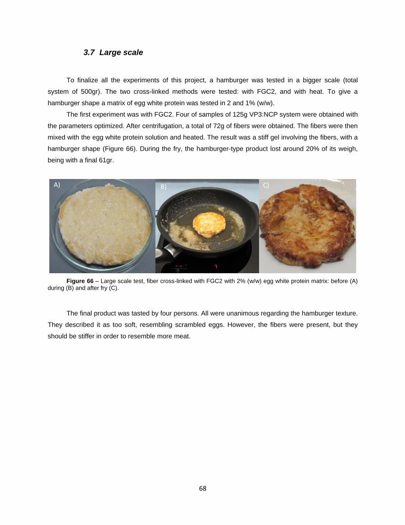
68

3.7 Large scale

To finalize all the experiments of this project, a hamburger was tested in a bigger scale (total

system of 500gr). The two cross-linked methods were tested: with FGC2, and with heat. To give a

hamburger shape a matrix of egg white protein was tested in 2 and 1% (w/w).

The first experiment was with FGC2. Four of samples of 125g VP3:NCP system were obtained with

the parameters optimized. After centrifugation, a total of 72g of fibers were obtained. The fibers were then

mixed with the egg white protein solution and heated. The result was a stiff gel involving the fibers, with a

hamburger shape (Figure 66). During the fry, the hamburger-type product lost around 20% of its weigh,

being with a final 61gr.

Figure 66 – Large scale test, fiber cross-linked with FGC2 with 2% (w/w) egg white protein matrix: before (A) during (B) and after fry (C).

The final product was tasted by four persons. All were unanimous regarding the hamburger texture.

They described it as too soft, resembling scrambled eggs. However, the fibers were present, but they

should be stiffer in order to resemble more meat.

A) B) C)

69

The last experiment was with heat as cross-linker. Six samples of 125g VP3:NCP system were

obtained with the parameters optimized. To improve the flavour, meat flavour was added to the fibers

before neutralization. As the last experiment was too soft, the centrifuged fibers were compressed to

remove the water. The result was 24 gr. of fibers, which were mixed with egg white protein and fried on a

pan (Figure 67).

Figure 67 – Large scale test, fiber cross-linked with 1% (w/w) heat and compressed, with egg white protein matrix: before (A) and after fry (B and C).

This final product was tasted by six persons. The texture was improved from the previous

experiment. This resembled more chicken, even though it was too dry. The egg flavour was not very

intensive anymore. Regarding the flavour, the opinions were diverse as some did not felt the meat

flavour.

A) B) C)

70

71

4 Conclusions

The main objective of this project was to understand the fiber formation with vegetable proteins,

resulting on a development of a new meat alternative. The product should resemble as much as possible

real meat in terms of bite (juiciness) and structure (presence of fibers). The system selected was

VP3:NCP since VP3 was the most soluble vegetable protein. The ratio that gave best results was 6:1.

Good water-retaining fibers were created by optimizing parameters in the coacervation process.

The acidification turned out to be a crucial step in obtaining well defined fibers. Slow acidification (18

hours) with GdL did not give the results expected, as fibers were not formed. The best results were

achieved with acidifying the system slowly (15 minutes) with a strong acid (HCl through a pump). The

microstructures obtained with this parameters were well defined water-retaining fibers. The stirring effect

also determines the type of structure formed. The results indicate that high speed stirring is preferable to

obtain better fibers.

Concerning the amount of protein retained by the fibers, we can conclude that the lower the final

pH more protein is retained by the fibers. Also most of the protein is retained in the fibers before

neutralization. After this, there is a lost in yield of wet fibers and also in the protein yield. More

cross-linkers should be tested in order to improve the yields after neutralization, since the final product

has to be profitable.

To stabilize the fibers, cross-linking by heat and by adding FGC2 were the methods selected.

These made the fibers stronger and resistant to pH 7. The optimum amount of NaOH to reach pH 7 was

also studied and selected.

The final objective of this project was not only to create fibers but also to give them the shape of a

familiar hamburger. To do that, several methods of creating a VP matrix were tested but none succeeded.

To improve the taste, experiments with sunflower oil were performed. The main goal was to

understand how did the oil particles interact with the fibers. The conclusions were that oil droplets are

retained inside the fibers and also addition of oil improves the yield. Therefore oil can be added directly

into the fibers to improve mouth taste.

Finally, two large scale experiment was performed and the best result was obtained with

compressed fibers in a matrix of 1% (w/w) egg white protein. The hamburger-type product turned out to

be very similar to a chicken hamburger, having nice strong fibers inside. In the future, more experiments

with different protein as matrix need to be performed in order to obtain a product made out of only

vegetable proteins.

72

73

5 References

Websites

1. The United States Meat Industry at a Glance. Available from: www.meatami.com, last visualization: 29

July 2011.

2. China's increased meat demand. Available from: www.nextgenerationfood.com/news, last

visualization: July 29 2011.

3. Rising Demand for Meat Takes Toll on Environment. Available from: www.npr.org, last visualization:

July 29 2011.

4. Global Demand For Meat and Ethanol Are Contributing to The Grain Price Surge. Available from:

www.businessinsider.com, last visualization: 29 July 2011.

5. Custo de produção da carne de suíno sobe e o preço pago cai. Available from:

http://g1.globo.com/economia/agronegocios, last visualization: 29 July 2011.

6. Melamine in Food. Available from: www.hud.ac.uk, last visualization: 2 August 2011.

Articles and Books

Bungenberg de Jong, H. G. and Kruyt, H. R., 1929, Coacervation (Partial miscibility in colloid systems),

Proc. Koninkl. Med. Akad. Wetershap, 32 849-856.

Dziezak, J. D., 1989, Fats, oils, and fat substitutes, Food Technol., 7 66-74.

Foegeding, E. A., Daubert, C. R., Drake, M. A., Essick, G., Trulsson, M., Vinyard, C., and van de Velde,

F., 2011, A comprehensive approach to understanding textural properties of semi- and soft-solid

foods, Journal of Texture Studies, 10.

Jungbunzlauer, Glucono-delta-Lactone: Uniqueness in acidification: Basel, Switzerland, 2008.

Maltais, A., Remondetto, G. E., Gonzalez, R., and Subirade, M., 2005, Formation of Soy Protein Isolate

Cold-set Gels: Protein and Salt Effects, Journal of food science, 70 (1): 67-73.

Menger, F. M., 2002, Supramolecular chemistry and self-assembly, PNAS, 99 4818-4822.

O'Kane, F. E., Molecular characterisation and heat-induced gelation of pea vicilin and legumin. 2004,

Wageningen.

74

Overbeek, J. T. G. and Voorn, M. J., 1957, Phase separation in polyelectrolyte solutions. Theory of

Complex Coacervation J. Cell. Comp. Physiol. , 49 (1 ): 7-26.

Schmitt, C., Sanchez, C., Desobry-Banon, S., and Hardy, J., 1998, Structure and Technofunctional

Properties of Protein-Polysaccharide Complexes: A Review, Critical Reviews in Food Science

and Nutrition, 38 (8): 689-753.

Smith, P. K., Krohn, R. I., THermanson, G. T., Mallia, A. K., Gartner, F. H., Provenzano, M. D., Fujimoto,

E. K., Goeke, N. M., Olson, B. J., and Klenk, D. C., 1985, Measurement of protein using

bicichoninic acid, Analytical Biochemistry, 150 (1): 76-85.

Sun, X. D. and Arntfield, S. D., 2011, Dynamic oscillatory rheologial measurement and thermal properties

of pea protein extracted by salt method: Effect of pH and NaCl, Journal of food engineering, 105

(3): 577-582.

Tainaka, K., 1980, Effect of counterions on complex coacervation, Biopolymers, 19 (1289-1298):

Thies, C., 1982, Microcapsules as drug delivery devices, Crit. Rev. Biomed. Eng, 8 335-383.

Tolstoguzov, V. B., 1991, Functional properties of food proteins and role of protein – polysaccharide

interaction, Food Hydrocolloids 4(6): 429-468.

Tolstoguzov, V. B., Izjumov, D. B., Grinberg, V. Y., Marusova, A. N., and Chekhovskaya, V. T., Methor of

Making Protein-Containing Foodstuffs Resembling Minced-Meat: United States Patent

Application 3,829,587, 1974.

Turgeon, S. L., Beaulieu, M., Schmitt, C., and Sanchez, C., 2003, Protein – polysaccharide interactions:

phase-ordeing kinetics, thermodynamic and structural aspects., Current opinion in colloid and

interface science 8401-414.

van de Velde, F. and Klok, H. J., 2011, The role of microstructure in texture perception, New Food, 14 (2):

53-56.

van de Velde, F. and Tromp, H., 2002, What does mouth feel look like?, Food Engineering & Ingredients,

December 38-43.

Vasbinder, A. J., Casein – whey protein interactions in heated milk, . Utrecht University: Utrecht, The

Netherlands, 2002.

Veis, A. and Aranyi, C., 1960, Phase separation in polyelectrolyte systems. I. Complex coacervates of

gelatine, J. Phys. Chem. , 64 :1203-1210.

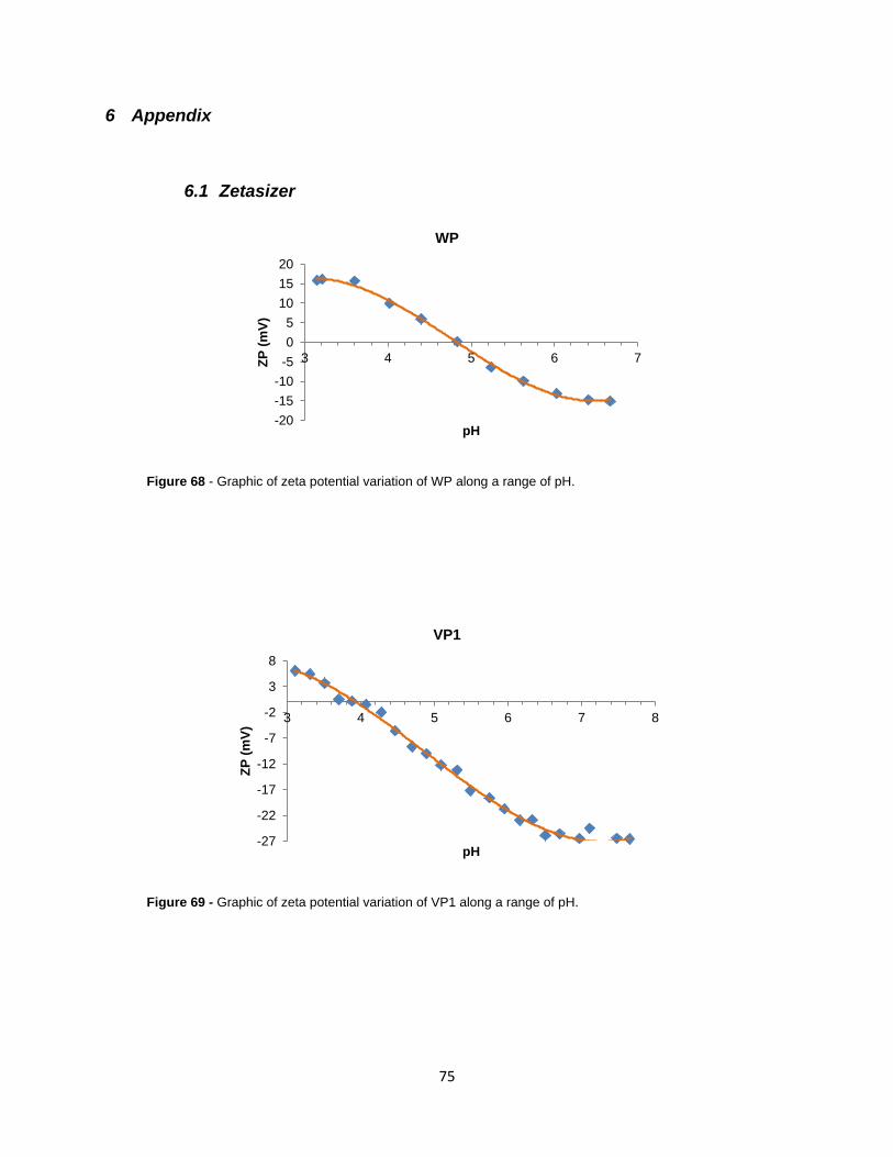
75

6 Appendix

6.1 Zetasizer

Figure 68 - Graphic of zeta potential variation of WP along a range of pH.

Figure 69 - Graphic of zeta potential variation of VP1 along a range of pH.

-20

-15

-10

-5

0

5

10

15

20

3 4 5 6 7ZP

(m

V)

pH

WP

-27

-22

-17

-12

-7

-2

3

8

3 4 5 6 7 8

ZP

(m

V)

pH

VP1

76

Figure 70 – Graph of zeta potential variation of VP3 along a range of pH.

Figure 71 - Graphic of zeta potential variation of VP4 along a range of pH.

Figure 72 - Graphic of zeta potential variation of NCP along a range of pH.

-20

-15

-10

-5

0

5

10

15

20

3.2 3.7 4.2 4.7 5.2 5.7 6.2ZP

(m

V)

pH

VP3

-25

-15

-5

5

15

25

3 4 5 6 7ZP

(m

V)

pH

VP4

-60

-50

-40

-30

-20

-10

0

2.5 3.5 4.5 5.5 6.5 7.5

ZP

(m

V)

pH

Xanthan

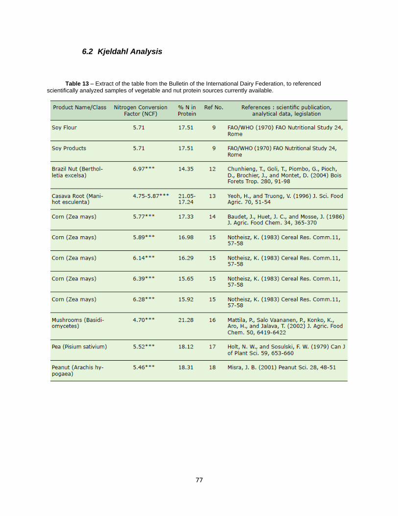
77

6.2 Kjeldahl Analysis

Table 13 – Extract of the table from the Bulletin of the International Dairy Federation, to referenced scientifically analyzed samples of vegetable and nut protein sources currently available.

78

6.3 Slow acidification with GdL

Figure 73 – Acidification profile for systems WP:NCP ratio 24:1 at 25ºC, using different GdL concentrations.

Figure 74 - Acidification profile for systems WP:NCP ratio 12:1 at 25ºC, using different GdL concentrations.

Figure 75 - Acidification profile for systems WP:NCP ratio 6:1 at 25ºC, using different GdL concentrations.

4

4.5

5

5.5

6

6.5

0 200 400 600 800 1000 1200 1400

pH

Time (min)

Acidification profile with GdL (25℃) 24:1 (WP/Xanthan)

0.30% GDL

0.45% GDL

0.50% GDL

0.65% GDL

0.75% GDL

0.80% GDL

4

4.5

5

5.5

6

6.5

0 200 400 600 800 1000 1200 1400

pH

Time (min)

Acidification profile with GdL (25℃) 12:1 (WP/Xanthan)

0.20% GDL

0.25% GDL

0.30% GDL

0.40% GDL

0.45% GDL

0.50% GDL

3.6

4.1

4.6

5.1

5.6

6.1

6.6

0 200 400 600 800 1000 1200 1400

pH

Time (min)

Acidification profile with GdL (25℃) 6:1 (WP/Xanthan)

0.10% GDL

0.15% GDL

0.20% GDL

0.25% GDL

0.30% GDL

0.35% GDL

0.40% GDL

79

Figure 76 - Graphic of the final pH achieved for each concentration of GdL, for WP and NCP ratio of 24:1 at

25ºC.

Figure 77- Graphic of the final pH achieved for each concentration of GdL, for WP and NCP ratio of 12:1 at 25ºC.

Figure 78 - Graphic of the final pH achieved for each concentration of GdL, for WP and NCP ratio of 6:1 at 25ºC.

y = -1.668x + 5.5191 R² = 0.972

4

4.2

4.4

4.6

4.8

5

5.2

0.20 0.40 0.60 0.80 1.00

Fin

al p

H

% GdL

WP:Xanthan 24:1

y = -2.3929x + 5.2692 R² = 0.9769

4

4.2

4.4

4.6

4.8

5

0.10 0.20 0.30 0.40 0.50

Fin

al p

H

% GdL

WP:Xanthan 12:1

y = -5.8071x + 5.9089 R² = 0.813

3.80

4.20

4.60

5.00

5.40

0.00 0.10 0.20 0.30 0.40

Fin

al

pH

% GdL

WP:Xanthan 6:1

80

6.4 BCA analysis

Figure 79 – Graphic of BCA results, with the standard curve and the interpolations of the protein concentrations in the experience of “influence of pH on the amount of protein inside the fibers”.

y = 0.0006x + 0.0375 R² = 0.9978

0.0

0.2

0.4

0.6

0.8

1.0

1.2

1.4

0 500 1000 1500 2000 2500

Ab

s 5

62 n

m

Protein (μg/ml)

BC Analysis to WP:Xanthan system

Calibration

24:1, pH 4.2

24:1, pH 4.8

6:1, pH 4.2

6:1, pH 4.8

81

Figure 80 – BCA protocol followed.