development of information products for rangeland managers
TRANSCRIPT

Seediscussions,stats,andauthorprofilesforthispublicationat:https://www.researchgate.net/publication/291206709
Developmentofinformationproductsforrangelandmanagers
TechnicalReport·April2001
DOI:10.13140/RG.2.1.1879.6565
CITATIONS
0
READS
7
1author:
AlexanderHolm
AlexanderHolm&Associates,FremantleWesternAustralia
33PUBLICATIONS574CITATIONS
SEEPROFILE
AllcontentfollowingthispagewasuploadedbyAlexanderHolmon20January2016.
Theuserhasrequestedenhancementofthedownloadedfile.

Development of Information Products for Rangeland Managers
NHT Project 953024
A contract with Agriculture Western Australia to develop and recommend
methods for the summary and presentation of Landscape Function Analysis
(LFA) data for the Western Australian Rangeland Monitoring System
(WARMS)
April 2001
Alexander Holm
Alexander Holm and Associates
26 Edward St
Nedlands
Western Australia

2
Executive Summary
Recommendations for LFA data presentation in standard WARMS reports and
for interpreting change in LFA data at the site scale.
1. Group WARMS vegetation types and pasture groups into five main country-
types based on vegetation structure and main mode of resource control:
hummock grassland, tussock grassland, southern sandplain, shrub-steppe and
mulga hardpan.
2. Classify each patch-type as resource-capturing or resource-shedding based on
definitions provided in this report.
3. From each transect log, calculate a resource-capturing index as one of the key
indicators of landscape function. RC Index = Σ length of resource-capturing
patches/total transect length
4. Calculate site-scale LFA indicators (stability, infiltration and nutrient cycling)
based on proportional lengths of patch-types and respective LFA ratings for
each patch-type.
5. Replace existing WARMS presentations of landscape function with a more
visual product. Examples of suggested presentations are provided in
Appendix 2
Recommendations for summarising, presenting and interpreting LFA change
data at the vegetation community / district level.
1. Examples of suggested summary tables and graphical presentations based on
vulnerability of the site to disturbance and changes in RC index and/or
stability rating are presented.
2. An interpretive matrix is provided based on the RC index and Stability rating.
Plotting the regional/vegetation type LFA profiles for WA rangelands and
recommendations on the importance of completing the curves for particular
vegetation types.
1. Some weak linear relationships, but no sigmoidal relationships, were found
between LFA ratings and disturbance indicators of distance from water,
grazing intensity and RC index.
2. It is unlikely that any further analysis of WARMS data using available
indicators of disturbance will greatly strengthen the relationships presented in
this report.
3. More sophisticated independent indicators of disturbance are required which
could include stocking histories associated with particular sites, selected to
cover the range of LFA ratings and RC indices. The likely success of such an

3
approach is problematic, especially given the very limited success of the
approach tested here and is not recommended.
4. Meanwhile, the approach adopted in this report based on frequency
distributions of sites is a reasonable first pass and will suffice until more data
becomes available or alternative approaches are identified.
Recommendations for frequency of LFA recordings.
1. Landscape function be assessed at each scheduled sampling i.e. every three to
four years on grassland sites and every five to six years on shrub-steppe sites.
Recommendations for cutting down the LFA sampling set.
1. Consider discontinuing infiltration/runoff and nutrient cycling ratings and
specific soil surface assessment attributes associated with these ratings i.e.
perennial plant cover (grassland), soil cover – flow (shrubland), litter source,
litter incorporation, microtopography and soil texture.
2. Soil surface assessment be restricted to resource-shedding patches (fetch) in
both grassland and shrubland sites.
3. Greater attention be given to classifying and logging patches as resource-
capturing and resource-shedding based on the definitions provided. All
significant fetch zone – types to be logged and sampled.
The relationship between LFA and vegetation data.
Importance of testing relationships between species composition and LFA.
1. Frequency cannot be used in place of transect logging to establish the RC
index.
2. Higher frequencies are associated with higher stability and infiltration ratings
on tussock grassland as expected, and in these situations provide
complementary information.
3. In general, shrub density provides complementary information on landscape
function, however this information is not sufficiently robust to be used with
confidence in reporting landscape function.
4. A provisional framework for interpreting change in species composition and
trends in landscape function is provided.
5. Two simultaneous sets of data are required to report change for pastoral
purposes, one set dealing with landscape function and the other with
vegetation change. While some inferences may be made between these data
sets, these two data sets should be assessed and reported independently.
6. Mounting a major research program to investigate relationships between
species composition and landscape function is not recommended.
4
Contents
Executive Summary ..................................................................................................... 2
Contents ........................................................................................................................ 4
Contract Brief: ............................................................................................................. 6
General approach ......................................................................................................... 7
Recommendations for LFA data presentation in standard WARMS reports. ...... 8
Defining reporting groups ......................................................................................... 8
Defining patch types .................................................................................................. 8
Calculation of site index of resource-capture ............................................................ 9
Calculation of LFA ratings for patch and site ........................................................... 9
Distribution of LFA ratings and resource-capturing indices .................................. 10
Recommendations for interpreting change in LFA data at the site scale. ............ 17
Background .............................................................................................................. 17
Thresholds in landscape function ............................................................................ 19
Presentation of landscape function data at site-scale ............................................. 19
Recommendations for summarising, presenting and interpreting LFA change
data at the vegetation community / district level. ................................................... 20
Plotting the regional/vegetation type LFA profiles for WA rangelands and
recommendations on the importance of completing the curves for particular
vegetation types .......................................................................................................... 22
Background: ............................................................................................................. 22
Approach .................................................................................................................. 22
Results ...................................................................................................................... 27
Recommendations: ................................................................................................... 30
Recommendations for how frequently LFA should be recorded .......................... 31
Background: ............................................................................................................. 31
Recommendation ...................................................................................................... 31
Recommendations for cutting down the LFA sampling set. .................................. 31
Background: ............................................................................................................. 31
Possible reduction in soil surface attributes that are assessed ............................... 31
Relationship between LFA ratings at patch and site-scales – shrub-steppe sites ... 32
Transect logging and simplification of fetch zones .................................................. 33
Recommendations .................................................................................................... 33

5
Relationship between LFA and vegetation data. .................................................... 34
Importance of testing the relationship between species composition and LFA. .. 34
Background .............................................................................................................. 34
Relationship between RC Index, LFA ratings and shrub density or perennial grass
frequency .................................................................................................................. 35
Approach .............................................................................................................. 35
Conclusion: .......................................................................................................... 35
Species composition and landscape function ........................................................... 44
Background .......................................................................................................... 44
Approach .............................................................................................................. 45
Relationships between reporting of landscape function and reporting for pastoral
production ................................................................................................................ 45
References ................................................................................................................... 47
Appendices .................................................................................................................. 48
Appendix 1 Frequency tables. .................................................................................. 48
Appendix 2: Examples of presentations of landscape function at the site scale ...... 55

6
Contract Brief:
The following tasks will be reported in a single document, which will act as the
contract report and its delivery will be considered the final milestone.
These tasks will be reviewed during the term of the contract, and the detail may be
amended, on the basis of recommendations from Dr Holm and in discussion with Dr
Watson.
The tasks apply to both WARMS SHRUBLANDS and GRASSLAND sites, although
in many cases the findings will be identical.
1) Recommendations for LFA data presentation in standard WARMS reports (i.e. as
produced by WARMS database).
1a) set of MS ACCESS queries to extract data as per recommendations in 1).
2) Recommendations for interpreting change in LFA data at the site scale. These will
be in the form of a set of “rules” weighting the relevant importance of various LFA
attributes recorded.
3) Recommendations for summarising, presenting and interpreting LFA change data
at the vegetation community / district level. Examples of such presentation will be
included.
4) Discussion of the relationship between LFA and vegetation data. Are they
indicating complementary changes, reinforcing similar interpretations or providing
information on different parameters?
5) Consider Tongway and Hindley's Audit recommendations in the context of
WARMS. How would one go about plotting the regional/vegetation type LFA profiles
for WA rangelands as Tongway and Hindley suggest? (AGWEST to supply Dr Holm
with a copy of Tongway and Hindley’s report, 2000).
6) Recommendations for how frequently LFA should be recorded within each of the
WARMS groups.
7) Recommendations for cutting down the LFA sampling set. For example, can 20%
of the attributes assessed give us 80% of the information required to show change?
8) Express some written views on how important it is to test the relationship between
species composition and LFA. If, after discussion between the Contractor and the
AGWEST Officer it is considered this is an important research question - draft a 1-2
page Preliminary Research Proposal for AGWEST to progress.
9) Based on 5 above, provide some recommendations on the importance of
completing the curves for particular vegetation types. If, after discussion between the
Contractor and the AGWEST Officer it is considered this is an important research
question - draft a 1-2 page Preliminary Research Proposal for AGWEST to progress.

7
General approach
WARMS and grassland data were provided by AGWEST in MS Access format.
Data was generally accepted as correct, however several errors were detected and
corrected during processing and Mr Philip Thomas advised.
In developing the suggested products I produced several tables in MS ACCESS as
examples of query outputs. My approach to MS ACCESS queries is a stepwise
process that does not lend itself to generation of one-pass query statements.
Therefore, I have not attempted to provide the queries themselves but have provided
detail on how the outputs are produced.
The outputs and tables are provided as examples, they are derived from ‘real’ data but
have not been checked and will contain errors. All outputs and tables should therefore
be rebuilt.
Statistical analyses were performed using SSPS (SPSS Inc, 1999) and graphs were
produced either in SSPS or in Sigma Plot.
Copies of all relevant outputs and tables are provided on CD.

8
Recommendations for LFA data presentation in standard WARMS reports.
Defining reporting groups
Monitoring sites have been classified on the basis of pasture groups (e.g. MSGF –
mulga short grass forb and WARMS groups (EB9 – mulga shrubland). These
groupings were used to allocate sites to the following broad country types (based on
structural form of the vegetation (e.g. clumps or groves) and transport mechanisms.
Table 1: Recommended country-type groups for landscape function reporting
Country type Landscape characteristics
Southern shrubland
Sandplain Individual shrubs and trees, clumps of shrubs and trees,
perennial grasses and/or spinifex. High infiltration rates with
little overland flow
Shrub-steppe Individual shrubs of clumps of shrubs, usually with few trees.
Sheet flow and wind transport.
Mulga hardpan Groves of shrubs and trees, individual shrubs and trees. Sheet
flow, broad drainage flow zones.
Grassland
Tussock grassland Individual tussocks or clumps of tussocks, few to many trees.
Hummock
grassland
Spinifex often with other perennial grasses, usually on deep
sandy soils.
Sites were allocated to these major groups, firstly on the basis of WARMS groupings
as shown in Table 2. Secondly, pasture groups were also allocated to country types
and used to modify the primary allocation. For example, sites allocated to WARMS
group EB9 contained sites on wandarrie banks, which were reallocated to ‘sandplain’.
Many sites were not classified either by WARMS group or pasture group. I used
transect data to classify some of these sites.
MS ACCESS table : alecpasture_groups.table
Defining patch types
Resource-capturing patches consist of perennial plants –living, standing dead and
fallen dead. The resource-capturing patches are the soil-surface footprints below
these plants where nutrient cycling is active, water infiltrates, and organic matter and
soil nutrients are concentrated. These patches maybe single plants, clumps, mats and
groves. Resource-shedding patches are the interspaces between the resource-
capturing patches where resources are more or less uniformly distributed. Annual
species dominate these patches. Measures of landscape patchiness have been shown
to provide good indicators of landscape function whereby loss of resource-capturing
patches often leads to loss of resources from the landscape, especially in non-resilient
landscapes.
9
Table 2: Allocation of WARMS groups to country types
WARMS Group Description Country type
EB1 Spinifex grassland Hummock grassland
EB2 Salt lakes, rocks and heath
EB3 Short bunch grass savanna Tussock grassland
EB4 Chenopod shrubland Shrub-steppe
EB5 Other Acacia woodland Sandplain
EB7 Eucalypt chenopod shrubland Shrub-steppe
EB9 Mulga shrubland Mulga hardpan
EB10 Nullarbor Shrub-steppe
NB1 Inaccessible hills, mud flats
NB2 Frontage grass Tussock grassland
NB3 Curly spinifex Tussock grassland
NB4 Pindan Tussock grassland
NB5 Mitchell grass Tussock grassland
NB6 Limestone grass Tussock grassland
NB8 Soft spinifex grassland Hummock grassland
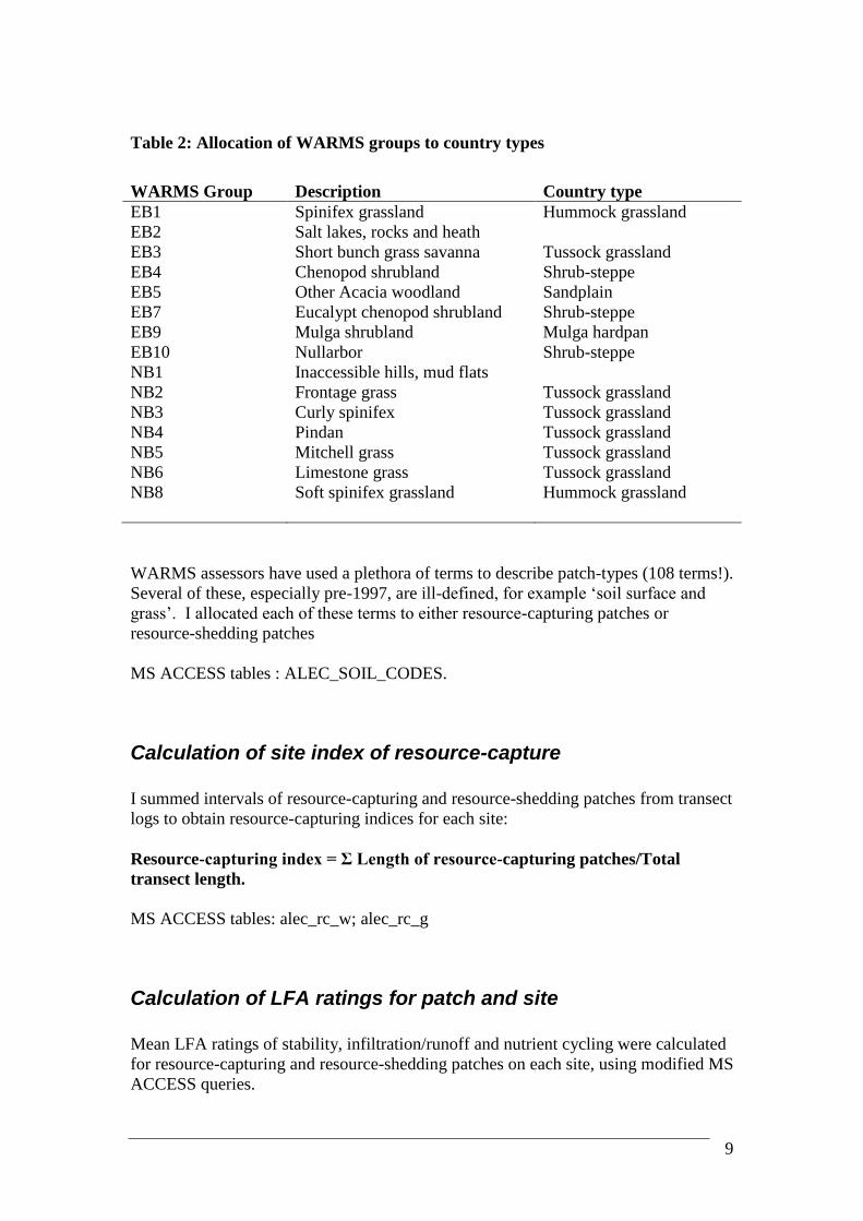
WARMS assessors have used a plethora of terms to describe patch-types (108 terms!).
Several of these, especially pre-1997, are ill-defined, for example ‘soil surface and
grass’. I allocated each of these terms to either resource-capturing patches or
resource-shedding patches
MS ACCESS tables : ALEC_SOIL_CODES.
Calculation of site index of resource-capture
I summed intervals of resource-capturing and resource-shedding patches from transect
logs to obtain resource-capturing indices for each site:
Resource-capturing index = Σ Length of resource-capturing patches/Total
transect length.
MS ACCESS tables: alec_rc_w; alec_rc_g
Calculation of LFA ratings for patch and site
Mean LFA ratings of stability, infiltration/runoff and nutrient cycling were calculated
for resource-capturing and resource-shedding patches on each site, using modified MS
ACCESS queries.

10
MS Access table alec_ratings_patch_g and alec_ratings_rc_patch_w
These LFA ratings were combined into site ratings by pro-rata based on the resource-
capturing index for each site.
Site LFA ratings (stability, infiltration, nutrient cycling) = LFA rating resource-
capturing patches X resource capturing index + LFA rating resource-shedding
patches X (1-resource capturing index).
Note, resource-capturing patches are not generally sampled in Grassland sites and site
LFA ratings were not calculated.
MS ACCESS table: alec_ratings_rc_site_w
Distribution of LFA ratings and resource-capturing indices
LFA ratings and resource-capturing indices for each date of recording were plotted as
frequency histograms (Figures 1-6). All LFA ratings were normally distributed,
while resource-capturing indices were strongly skewed in that there were far more
sites with low scores. Distribution patterns for WARMS sandplain and mulga-
hardpan country-types were similar and these have plotted together.

11
Figure 1: Frequency distribution of LFA ratings for shrubland monitoring sites –
shrub steppe country type

12
Figure 2: Frequency distribution of LFA ratings on shrubland sites – sandplain and
mulga
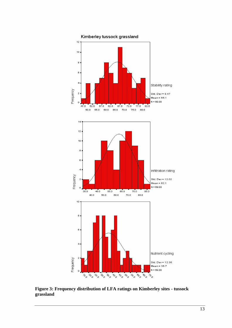
13
Figure 3: Frequency distribution of LFA ratings on Kimberley sites - tussock
grassland
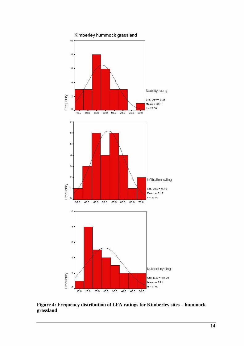
14
Figure 4: Frequency distribution of LFA ratings for Kimberley sites – hummock
grassland

15
Figure 5: Frequency distributions of resource-capturing indices (RC index) on
southern monitoring sites.

16
Figure 6: Frequency distributions of resource-capturing indices (RC index) of
Kimberley sites

17
Recommendations for interpreting change in LFA data at the site scale.
Background
Landscape function at the site-scale maybe inferred from both LFA ratings (stability,
infiltration/runoff and nutrient cycling) and indices of resource-capture. Additional
information maybe derived from density of shrubs or frequency of perennial grasses, and
this will be discussed under point 4. I suggest that temporal variability of each of these
ratings and indices is likely to be significantly different and will influence how change is
interpreted (Table 3)
Interpretation of change in nutrient cycling rating is likely to be seasonally dependent and
highly uncertain, especially with infrequent sampling. I therefore recommend that less
importance be given to change in nutrient cycling ratings.
Infiltration rating depends on soil texture and slaking (largely invariant), microtopography
(uncertain properties under grazing or other disturbance), soil cover (related to resource-
capturing index but confounded by inclusion of rocks and other invariant features), and
litter cover (seasonally dependent). While the infiltration rating for the site provides
useful information on how the site might respond to rainfall, it is difficult to interpret
change in this rating. Again, I recommend less importance be given to change in
infiltration rating.
Stability rating is composed of several indicators that are related to grazing in
complementary ways and with similar temporal variance. I recommend greater
importance be given to change in stability rating.
As mentioned before, grazing directly influences change in RC index. However, these
changes must be interpreted within a broad-scale understanding of structural transitions
such as change from grassland to shrubland or fine-scale shrubland to coarse-scale
shrubland. Thus grazing may initially result in loss of perennial shrubs or grasses and
consequent decline in RC index. Subsequently however, these degraded landscapes may
be resorted at broader scales, associated with ingress of other species, and the restoring of
RC index and landscape function.
A framework to interpret change in landscape function is recommended based on the RC
index and stability rating (Table 4). Interpretation is maybe aided by vegetation
information, which is discussed later.
Change is arbitrarily (but leniently) defined as greater than one standard deviation
difference in either RC index or stability rating between sampling dates.
All sites that were below both the median RC index and Stability rating were classed as
vulnerable to disturbance while others were either less vulnerable or resilient to
disturbance.
MS ACCESS tables: alec_rc_ratings_w; alec_function_dens_change_9500;

18
Table 3: Likely temporal variability in ratings and indices of landscape function and
soil surface indicators
Landscape function
indicators
Temporal variability Comment
Resource-capturing index Very low Trends evident >5 years –
changes grazing induced
Ratings:
Stability Low Soil and litter cover variable
other soil surface factors much
less variable
Infiltration/runoff Low Litter cover variable, others
much less variable
Nutrient cycling High Especially on resource-shedding
patches
Soil surface indicators
Soil cover (interception) Moderate Related to RC index and to
seasonal conditions
Soil cover (overland flow) Low Related to RC index but also
includes rocks and other
invariant objects
Crust broken-ness Low-moderate Probably influenced by grazing
Cryptogam cover Low-moderate Influenced by grazing,
confounded by litter (ie high
litter – low cryptogams)
Erosion features Low Grazing induced
Eroded materials Low Grazing induced
Litter cover High Seasonally dependent
Litter origin High Seasonally dependent
Litter incorporation Low – moderate Disproportionate effect on rating
Soil microtopography Low Largely invariant, some grazing
impact
Surface nature Low Uncertain relationship to
grazing or other disturbance
Slake test Very low Grazing exposes sodic soils
Soil texture Very low Mostly invariant.

19
Table 4 An interpretive framework for assessing change in landscape function
Stability rating RC index RC index
Low - -ve change* Medium-high - ve change
Low Highly
vulnerable to
further
disturbance
Requires
urgent
remedial action
Moderately
vulnerable to
disturbance
Alert –
precautionary
action
recommended
High Degraded but
stable and
probably
productive
Alert –
precautionary
action
recommended
Stable Noted
* Negative change in either or both stability and RC index. Contradictory changes are
less urgent.
Thresholds in landscape function
Later in this report (point 5/9) I investigate sigmoidal response curves in landscape
function as suggested by Tongway and Hindley (2000). No significant relationships were
established. Alternatively, I have suggested thresholds for the main country types based
subjectively on the frequency distributions. These thresholds are provisionally set at the
modal value (e.g. Figure 5 and Figure 6).
Presentation of landscape function data at site-scale
I recommend existing WARMS presentations of landscape function be replaced with a
more visual product. Examples of suggested presentations are provided in Appendix 2

20
Recommendations for summarising, presenting and interpreting LFA change data at the vegetation community / district level.
Summary tables and graphical presentations based on vulnerability of the site to
disturbance and changes in RC index and/or stability index are proposed.
I suggest the data be presented within the five structural country types (southern
sandplain, shrub-steppe, mulga hardpan, hummock grassland communities and tussock
grassland). Data maybe further sub-divided at district levels when sufficient sites have
been re-sampled, although it is possible to allocate all sites to vulnerability classes on the
basis of one sampling.
An example presentation for the southern rangeland is presented in Table 5. Sites shown
as changing significantly, were those with changes greater than one SD in either RC Index
or stability rating.
MS ACCESS tables: alec_rc_ratings_w; alec_function_dens_change_9500;
alec_regionalsummary_w
Table 5 Landscape function status of WARMS sites in southern rangeland of
Western Australia sampled between 1995 and 2000 and trends in landscape function
of re-sampled sites
Total sites
Vulnerability of site to
disturbance Re-sampled
1999/2000
Significant
change Moderate to
High
Low or
stable
Number of sites and percentages
Sandplain 35 13 37% 22 63% 8 23% 2 (25%) ↑
6 (75%) NC
Shrub-
steppe
593 187 32% 406 68% 19 3% 2 (10%) ↑
1 (5%) ↓
16 (85%) NC
Mulga
hardpan
119 35 29% 84 71% 10 8% 1 (10%) ↓
9 (90%) NC
A suggested graphical presentation of this same data is provided in Figure 7. In this
presentation, sites are arranged along the X axis 1) within broad categories of
vulnerability to disturbance based on Table 4, modal thresholds in RC Index and Stability
rating were used to establish the four categories; and 2) by ranking on RC index – i.e.
lowest ranking sites to the left.

21
Figure 7: Regional trends in landscape function (differences in resource-capturing
index) in monitoring sites in the southern rangeland. Sites are arranged along the X
axis from most to least vulnerable to disturbance. Sites changing greater than one
SD (dotted line) are considered to have changed significantly.

22
Plotting the regional/vegetation type LFA profiles for WA rangelands as Tongway and Hindley suggest and provide recommendations on the importance of completing the curves for particular vegetation types
Background:
Tongway and Hindley (2000) suggest that ‘establishing the changes in landscape function
in response to change of stresses and disturbances, in the form of a landscape function
curve, is of paramount importance.’ Further, they suggest that sigmoidal response curves
be fitted to establish thresholds where there are sharp discontinuities between landscape
function and disturbance. Such thresholds are intuitively appealing and have been
suggested for several years (Friedel, 1991), but there has been no progress on their
derivation. Attempts to relate LFA ratings to various disturbance indicators (soil nutrients
and RC index) in Western Australian rangeland have been previously unsuccessful (Holm
et al., 2001). On the other hand, there was a significant relationship between soil
nutrients and RC index in this study, however this was not sigmoidal.
Approach
One of the difficulties in attempting to derive these relationships between disturbance and
landscape function, is to quantify ‘disturbance’ in non-experimental situations.
For this report, I used data from the WARMS sites to establish RC index, frequency of
perennial grass, (both log transformed), distance from water, and a derived index of
grazing intensity (10/distance from water squared) as surrogates for disturbance from
grazing, and plotted these against LFA ratings. I also examined the relationship between
RC index and the other surrogates of grazing intensity. Both linear and sigmoidal
relationships were examined. I also used multiple regression approaches using country
type, RC index, frequency or shrub density, grazing intensity and salinity of water as the
variables likely to affect each of the LFA ratings

23
Figure 8: Relationship between LFA ratings and grazing intensity (10/distance from
water squared) for Kimberley grassland sites

24
Figure 9: Relationship between LFA ratings and grazing intensity (10/distance from
water squared) for shrubland monitoring sites in southern rangeland. Some
extreme values not shown.

25
Figure 10: Relationship between LFA ratings and resource-capturing index
(expressed as log RC Index X 100) for Kimberley grassland sites.

26
Figure 11: Relationship between LFA ratings and resource-capturing index for
shrubland monitoring sites in southern rangeland.

27
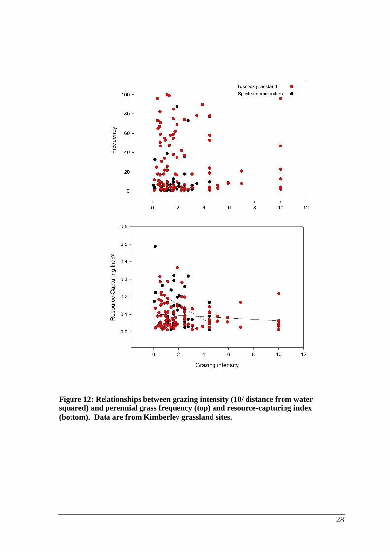
Results
Most relationships between LFA ratings and the surrogate variables of disturbance were
non-significant (Figure 8 - Figure 11). The few exceptions were stability and grazing
intensity on tussock grassland, which were negatively related (r2 = 0.11, p = 0.007 Figure
8). RC index was weakly negatively related to grazing intensity on hummock grassland
sites (r2 = 0.16; p = 0.016 Figure 12), and on shrub-steppe sites (r
2 = 0.01; p = 0.02 Figure
13) i.e. sites closer to water generally had lower RC Indices.
There were no sigmoidal relationships between indices or ratings of landscape function
and indices of disturbance.
Multiple regression analyses also failed to establish any strong relationships between LFA
ratings and disturbance indictors (Table 6)
Table 6: Multiple regression relationships between indictors of landscape function
and variables likely to affect disturbance by grazing. Relationships derived from
data collected on WARMS sites from 1992 – 2000
Landscape
function
indicator/rating
Significant terms Variance
accounted for
by model
Significance
of model
(p)
Grassland sites
Stability 78.5 2.8 –9.4 1.8 (if hummock grassl.) –
1.0 0.4 grazing intensity
0.26 0.000
Infiltration/runoff 70.1 4.2 + 0.08 0.04 frequency – 22.1
12.8 RC Index – 8.1 2.7 (if hummock
grassl.)
0.24 0.000
Nutrient cycling 44.0 3.6 – 7.2 2.6 (if hummock grassl.) 0.08 0.007
RC index 0.06 0.03 + 0.06 0.02 (if hummock
grassl.) – 0.007 0.003 grazing intensity –
0.0005 0.000 frequency
0.16 0.000
Shrub-steppe sites
Stability 62.1 0.4 + 0.0001 0.000 density – 2.2
1.3 (if sandplain) + 1.6 0.8 (if mulga)
0.02 0.05
Infiltration/runoff 50.0 0.5 – 0.003 0.000 salinity 0.01 0.04
Nutrient cycling 34.7 0.4 + 0.0002 0.000 density 0.02 0.001
RC index 0.15 0.01 + 0.00005 0.000 density +
0.06 0.01 (if shrub-steppe) + 0.004
0.002 grazing intensity
0.16 0.000
28
Figure 12: Relationships between grazing intensity (10/ distance from water
squared) and perennial grass frequency (top) and resource-capturing index
(bottom). Data are from Kimberley grassland sites.

29
Figure 13: Relationship between grazing intensity (10/distance from water squared)
and resource-capturing index (expressed as log RC Index x 100), for shrubland sites.

30
Recommendations:
It is unlikely that any further analysis of WARMS data will greatly strengthen these
relationships using available indicators of disturbance. More sophisticated independent
indicators of disturbance are required which could include stocking histories associated
with particular sites, selected to cover the range of LFA ratings and RC indices. The
likely success of such an approach is problematic, especially given the very limited
success of the approach tested here.
Meanwhile, the approach adopted in this report based on frequency distributions of sites is
a reasonable first pass and will suffice until more data becomes available or alternative
approaches are identified.

31
Recommendations for how frequently LFA should be recorded within each of the WARMS groups.
Background:
Assessment of change on monitoring sites requires simultaneous information on both
changes in biological capacity of sites to support the selected land use (e.g. change in
species composition is important for grazing), and changes in physical or geophysical
capacity of landscapes to support vegetation (landscape function).
Recommendation
Landscape function be assessed at each scheduled sampling i.e. every three to four years
on grassland sites and every five to six years on shrub-steppe sites.
Recommendations for cutting down the LFA sampling set.
Background:
Landscape function assessment requires both a measure of patchiness (Resource-
capturing index) and soil surface attributes –i.e. the current approach of transect logging
and LFA soil surface assessment (Tongway, 1994; Tongway & Hindley, 1995). I suggest
some modifications to these assessments that if adopted, will reduce the time required to
complete these assessments, but only by a matter of minutes per site.
Possible reduction in soil surface attributes that are assessed
If the recommendations within this report are adopted, then less importance will be placed
on the infiltration/runoff and nutrient cycling ratings and more importance on the RC
index and stability rating. This could be taken to the extreme whereby, all soil surface
assessment indicators not associated with stability rating could be dropped. These are:
perennial plant cover (grassland), soil cover – flow (shrub-steppe), litter source, litter
incorporation, microtopography and soil texture.

32
Relationship between LFA ratings at patch and site-scales – shrub-steppe sites
Tongway and Hindley (1995) do not assess the resource-capturing patches (i.e. perennial
grass butts) in their LFA analysis of grassland sites. In their view, ‘the quality of soil
associated with a perennial grass is high and does not vary much with overall site
condition; the big variation is in the quality of the fetch zones’ (fetch zones analogous
with resource-shedding patches). This raises the question, whether LFA assessments in
shrubland might also be restricted to the resource-shedding patches without serious loss of
information. Certainly the errors associated with measurement and spatial variability of
these measurements are likely to be higher within the resource-capturing patches.
I examined correlations between the LFA ratings within resource-capturing and resource-
shedding patches for WARMS shrub-steppe sites (Table 7). In general equivalent ratings
were highly correlated (r = 0.65 – 0.73), suggesting that most of the information could be
derived from only assessments of resource-shedding patches. I have presented frequency
tables of for both site-scale and patch-scale ratings and suggest that presentations be based
on resource-shedding patches for both grassland and shrub-steppe sites (Appendix 1).
Table 7: Correlations between LFA ratings for resource-capturing patches and
resource-shedding patches in shrubland monitoring sites
Resource-shedding patches Resource-capturing patches
Stability Infiltration Nutrient Stability Infiltration Nutrient
Resource- shedding
Stability Correlation 1.000 .479 .547 .698 .285 .314 Sig. (2-tailed) . .000 .000 .000 .000 .000 N 932 932 932 932 932 932 Infiltration Correlation 1.000 .310 .279 .730 .207 Sig. (2-tailed) .000 .000 .000 .000 N 932 932 932 932 Nutrient Correlation 1.000 .407 .199 .647 Sig. (2-tailed) .000 .000 .000 N 932 932 932
Resource- capturing
Stability Correlation 1.000 .455 .541 Sig. (2-tailed) .000 .000 N 932 932 Infiltration Correlation 1.000 .452 Sig. (2-tailed) .000 N 932 Nutrient Correlation 1.000 Sig. (2-tailed) N

33
Transect logging and simplification of fetch zones
As discussed previously, patch types along site transects are to be classified firstly as
either resource-capturing or resource-shedding (i.e. fetch) based on the definitions
provided in section 1. Tongway and Hindley (1995) then require fetch zones to be further
sub-divided into fetch zone-types and recommend a minimum of 5 queries per fetch-zone
type. Excessive splitting of fetch-zones is not recommended. There is no point in logging
a zone type if it is too small to be sampled. For example, the occasional ant bed that
occupies less than say 5% of the monitoring site should be excluded. Conversely, if a
zone-type is significant, it must be logged and sampled to enable calculation of LFA
ratings for the site based on the proportional lengths of each fetch-zone type.
Recommendations
1. Consideration be given to discontinuing infiltration/runoff and nutrient cycling
ratings and the specific soil surface assessment attributes associated with these
ratings i.e. perennial plant cover (grassland), soil cover – flow (shrubland), litter
source, litter incorporation, microtopography and soil texture.
2. Soil surface assessment be restricted to resource-shedding patches (fetch) in both
grassland and shrubland sites.
3. Greater attention be given to classifying and logging patches as resource-capturing
and resource-shedding based on the definitions provided. All significant fetch
zone – types to be logged and sampled.

34
Relationship between LFA and vegetation data.
Importance of testing the relationship between species composition and LFA.
Background
Increasingly, monitoring of the environment is seen to involve firstly an assessment of the
capacity of the landscape to convert rainfall into plant biomass (landscape function) and
secondly an assessment of the biodiversity that these landscapes support. While a
common approach to assessment is reasonable for all land uses in the first phase,
assessment techniques for the second phase depend on the nature of the land use. Thus,
on pastoral land used for grazing, biodiversity assessment requires a focus on changes in
species composition that affects grazing value. Such changes include loss of useful
perennial species and replacement of these species by unpalatable species, or herbaceous
annuals. Many of these transitions do not necessarily result in loss of landscape function
– the efficiency of conversion of rainfall into biomass is maintained on so-called resilient
landscapes. On less resilient landscapes, loss of perennial species precipitates significant
soil loss, and accelerated runoff resulting in loss of landscape function – i.e. lower
efficiency of conversion of rainfall into biomass. In time, even non-resilient landscapes
may again stabilize and become re-vegetated with alternative species often at broader
spatial scales. Interpretation of monitoring data from land used for pastoralism therefore
requires an understanding of where a monitoring site sits within the transition matrix and
must include data on landscape function and species composition.
A key indicator of landscape function is change in the proportional area occupied by
resource-capturing patches i.e. patches predominately occupied by perennial shrubs trees
and/or grasses – RC Index. Additional information on soil surface properties is required
to reveal if loss of patches is associated with accelerated soil loss or if the landscape is
stable and losses are minimal.
The questions addressed in this section include:
1. Is there a relationship between RC Index (as an indicator of landscape function)
and shrub density or perennial grass frequency?
2. Are LFA ratings related to shrub density or perennial grass frequency?
3. Is species composition related to landscape function?
4. Provide a framework for interpreting change in landscape function and in species
diversity and/or abundance.

35
Relationship between RC Index, LFA ratings and shrub density or perennial grass frequency
Approach
I examined these relationships using correlation and regression analyses of all available
site data for resource-shedding patches on all monitoring sites and on resource-capturing
patches on shrubland sites.
Unexpectedly, frequency of perennial grass was negatively correlated with resource-
capturing index on both hummock grassland (logs; - 0.24 p = 0.004) and tussock
grassland although the later was not significant. (Table 8 and Table 9).
Frequency of perennial grass was significantly correlated with LFA ratings for stability
and infiltration/runoff, but not nutrient cycling on both hummock grassland and tussock
grassland (Table 8 and Table 9).
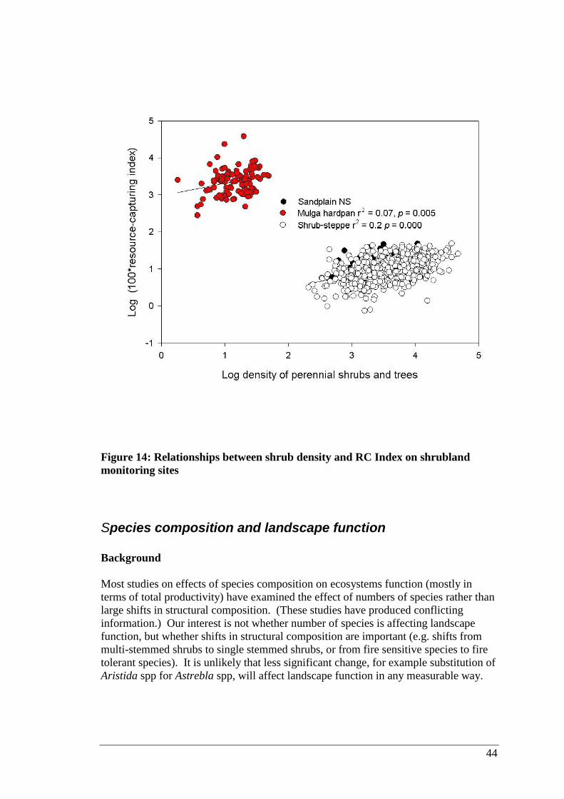
On resource-shedding patches, density of shrubs and trees was significantly positively
correlated with resource-capturing index on all country-types (sandplain: Table 10, shrub-
steppe: Table 11and mulga hardpanTable 12). Regression analysis indicates that these
relationships are strongest on shrub-steppe Figure 14). There was generally no correlation
between density and LFA ratings (Table 10 -Table 12). There were only marginal
differences in these correlations for resource-capturing patches (Table 13 - Table 15
Conclusion:
It might be expected that higher frequency or density of perennial species and all
indicators of landscape function should be positively related. More perennial grass or
shrubs should result in higher infiltration, more nutrient cycling and less movement of soil
and soil nutrients. Furthermore, one would expect resource-capturing index on a site to be
positively related to the frequency or density of plants.
On grassland monitoring sites, perennial grass frequency provides confusing information
about landscape function. Generally the higher frequencies are associated with lower RC
indices, although this is highly variable. My only explanation for this is that perhaps
higher frequencies indicate smaller plants with smaller basal areas. Whatever the
explanation, it is apparent that frequency cannot be used in place of transect logging to
establish the RC index. On the other hand, higher frequencies are associated with higher
stability and infiltration ratings on tussock grassland as expected, and in these situations
provide complementary information.
On southern monitoring sites, shrub density is associated with higher RC indices, but
associations with LFA ratings are weak or non-existent. It might be expected that the
associations with LFA ratings should be stronger in resource-capturing patches where
shrubs directly influence infiltration, nutrient cycling and perhaps stability. There is some
suggestion that this is so in shrub-steppe country-types but the correlations are weak.
In general, shrub density does provide complementary information on landscape function,
however this information is not sufficiently robust to be used with confidence in
reporting.

36
Table 8: Correlations (Pearson) among variables recorded on Kimberley grassland sites: tussock grassland – shed patches
Frequency Log freq RC Index Log RC I Stability Infiltration Nutrient Distance Grazing Int
Frequency Correlation 1.000 .886 .004 -.083 .112 .261 -.016 .050 -.059 Sig. (2-tailed) . .000 .966 .395 .358 .030 .894 .620 .559 N 107 107 107 107 69 69 69 100 100
Log freq Correlation .886 1.000 -.047 -.134 .178 .218 -.006 .051 -.045 Sig. (2-tailed) .000 . .628 .170 .144 .071 .964 .615 .658 N 107 107 107 107 69 69 69 100 100
RC Index Correlation .004 -.047 1.000 .894 -.281 -.298 -.179 .077 -.126 Sig. (2-tailed) .966 .628 . .000 .019 .013 .142 .446 .212 N 107 107 107 107 69 69 69 100 100
Log RC I Correlation -.083 -.134 .894 1.000 -.213 -.256 -.140 .050 -.117 Sig. (2-tailed) .395 .170 .000 . .079 .033 .251 .622 .247 N 107 107 107 107 69 69 69 100 100
Stability Correlation .112 .178 -.281 -.213 1.000 .573 .700 .317 -.335 Sig. (2-tailed) .358 .144 .019 .079 . .000 .000 .011 .007 N 69 69 69 69 69 69 69 64 64
Infiltration Correlation .261 .218 -.298 -.256 .573 1.000 .713 .131 -.085 Sig. (2-tailed) .030 .071 .013 .033 .000 . .000 .304 .505 N 69 69 69 69 69 69 69 64 64
Nutrient Correlation -.016 -.006 -.179 -.140 .700 .713 1.000 .025 -.083 Sig. (2-tailed) .894 .964 .142 .251 .000 .000 . .846 .515 N 69 69 69 69 69 69 69 64 64
Distance Correlation .050 .051 .077 .050 .317 .131 .025 1.000 -.700 Sig. (2-tailed) .620 .615 .446 .622 .011 .304 .846 . .000 N 100 100 100 100 64 64 64 100 100
Grazing Int Correlation -.059 -.045 -.126 -.117 -.335 -.085 -.083 -.700 1.000 Sig. (2-tailed) .559 .658 .212 .247 .007 .505 .515 .000 . N 100 100 100 100 64 64 64 100 100

37
Table 9 Correlations (Pearson) among variables recorded on Kimberley grassland sites: hummock grassland – shed patches
Frequency Log freq RC Index Log RC I Stability Infiltration Nutrient Distance Grazing Int
Frequency Correlation 1.000 .839 -.293 -.392 -.002 .038 .140 -.124 .205 Sig. (2-tailed) . .000 .083 .016 .994 .849 .485 .464 .223 N 37 37 36 37 27 27 27 37 37
Log freq Correlation .839 1.000 -.245 -.302 .051 .021 .173 -.022 .099 Sig. (2-tailed) .000 . .150 .070 .801 .918 .389 .898 .558 N 37 37 36 37 27 27 27 37 37
RC Index Correlation -.293 -.245 1.000 .894 .045 -.190 -.020 .404 -.399 Sig. (2-tailed) .083 .150 . .000 .827 .353 .921 .015 .016 N 36 36 36 36 26 26 26 36 36
Log RC I Correlation -.392 -.302 .894 1.000 .118 -.270 -.286 .227 -.231 Sig. (2-tailed) .016 .070 .000 . .558 .173 .148 .176 .170 N 37 37 36 37 27 27 27 37 37
Stability Correlation -.002 .051 .045 .118 1.000 .713 .665 -.108 .031 Sig. (2-tailed) .994 .801 .827 .558 . .000 .000 .590 .879 N 27 27 26 27 27 27 27 27 27
Infiltration Correlation .038 .021 -.190 -.270 .713 1.000 .868 -.114 .032 Sig. (2-tailed) .849 .918 .353 .173 .000 . .000 .571 .875 N 27 27 26 27 27 27 27 27 27
Nutrient Correlation .140 .173 -.020 -.286 .665 .868 1.000 .085 -.201 Sig. (2-tailed) .485 .389 .921 .148 .000 .000 . .673 .314 N 27 27 26 27 27 27 27 27 27
Distance Correlation -.124 -.022 .404 .227 -.108 -.114 .085 1.000 -.733 Sig. (2-tailed) .464 .898 .015 .176 .590 .571 .673 . .000 N 37 37 36 37 27 27 27 37 37
Grazing Int Correlation .205 .099 -.399 -.231 .031 .032 -.201 -.733 1.000 Sig. (2-tailed) .223 .558 .016 .170 .879 .875 .314 .000 . N 37 37 36 37 27 27 27 37 37

38
Table 10: Correlations (Pearson) among variables recorded on shrubland monitoring sites: sandplain - shed patches
Density RC Index Stability Infiltration Nutrient Log den Log RC I Distance Grazing Int Salinity
Density Correlation 1.000 .392 .086 .238 .223 .911 .274 -.050 .125 .206 Sig. (2-tailed) . .015 .543 .086 .109 .000 .096 .769 .462 .251 N 53 38 53 53 53 53 38 37 37 33
RC Index Correlation .392 1.000 .068 .150 .064 .395 .936 -.146 .139 .345 Sig. (2-tailed) .015 . .686 .370 .702 .014 .000 .388 .413 .050 N 38 38 38 38 38 38 38 37 37 33
Stability Correlation .086 .068 1.000 .404 .318 .111 -.019 -.135 .171 -.427 Sig. (2-tailed) .543 .686 . .003 .020 .427 .908 .427 .312 .013 N 53 38 53 53 53 53 38 37 37 33
Infiltration Correlation .238 .150 .404 1.000 .333 .234 .177 .147 -.097 -.017 Sig. (2-tailed) .086 .370 .003 . .015 .092 .287 .385 .567 .926 N 53 38 53 53 53 53 38 37 37 33
Nutrient Correlation .223 .064 .318 .333 1.000 .220 .067 .011 .210 -.182 Sig. (2-tailed) .109 .702 .020 .015 . .114 .690 .948 .211 .310 N 53 38 53 53 53 53 38 37 37 33
Log den Correlation .911 .395 .111 .234 .220 1.000 .325 .019 .071 .130 Sig. (2-tailed) .000 .014 .427 .092 .114 . .046 .913 .675 .470 N 53 38 53 53 53 53 38 37 37 33
Log RC I Correlation .274 .936 -.019 .177 .067 .325 1.000 -.066 .064 .394 Sig. (2-tailed) .096 .000 .908 .287 .690 .046 . .698 .705 .023 N 38 38 38 38 38 38 38 37 37 33
Distance Correlation -.050 -.146 -.135 .147 .011 .019 -.066 1.000 -.757 -.046 Sig. (2-tailed) .769 .388 .427 .385 .948 .913 .698 . .000 .798 N 37 37 37 37 37 37 37 37 37 33
Grazing Int Correlation .125 .139 .171 -.097 .210 .071 .064 -.757 1.000 -.110 Sig. (2-tailed) .462 .413 .312 .567 .211 .675 .705 .000 . .544 N 37 37 37 37 37 37 37 37 37 33
Salinity Correlation .206 .345 -.427 -.017 -.182 .130 .394 -.046 -.110 1.000 Sig. (2-tailed) .251 .050 .013 .926 .310 .470 .023 .798 .544 . N 33 33 33 33 33 33 33 33 33 33

39
Table 11 Correlations (Pearson) among variables recorded on shrubland monitoring sites: shrub-steppe – shed patches
Density RC Index Stability Infiltration Nutrient Log den Log RC I Distance Grazing Int Salinity
Density Correlation 1.000 .265 .069 .017 .148 .838 .337 -.078 .088 .136 Sig. (2-tailed) . .000 .061 .637 .000 .000 .000 .072 .043 .005 N 732 564 732 732 732 732 564 537 535 433
RC Index Correlation .265 1.000 -.020 -.010 .027 .278 .860 -.046 .076 .074 Sig. (2-tailed) .000 . .621 .815 .508 .000 .000 .276 .068 .112 N 564 605 605 605 605 564 605 571 569 458
Stability Correlation .069 -.020 1.000 .507 .493 .053 -.019 .050 -.038 .039 Sig. (2-tailed) .061 .621 . .000 .000 .149 .632 .230 .370 .406 N 732 605 776 776 776 732 605 571 569 458
Infiltration Correlation .017 -.010 .507 1.000 .281 -.007 -.023 .059 -.021 -.094 Sig. (2-tailed) .637 .815 .000 . .000 .847 .571 .157 .622 .044 N 732 605 776 776 776 732 605 571 569 458
Nutrient Correlation .148 .027 .493 .281 1.000 .136 .042 -.005 -.027 .039 Sig. (2-tailed) .000 .508 .000 .000 . .000 .301 .909 .525 .403 N 732 605 776 776 776 732 605 571 569 458
Log den Correlation .838 .278 .053 -.007 .136 1.000 .397 -.047 .083 .137 Sig. (2-tailed) .000 .000 .149 .847 .000 . .000 .278 .056 .004 N 732 564 732 732 732 732 564 537 535 433
Log RC I Correlation .337 .860 -.019 -.023 .042 .397 1.000 -.035 .070 .121 Sig. (2-tailed) .000 .000 .632 .571 .301 .000 . .410 .095 .010 N 564 605 605 605 605 564 605 571 569 458
Distance Correlation -.078 -.046 .050 .059 -.005 -.047 -.035 1.000 -.637 -.020 Sig. (2-tailed) .072 .276 .230 .157 .909 .278 .410 . .000 .671 N 537 571 571 571 571 537 571 571 569 454
Grazing Int Correlation .088 .076 -.038 -.021 -.027 .083 .070 -.637 1.000 .003 Sig. (2-tailed) .043 .068 .370 .622 .525 .056 .095 .000 . .947 N 535 569 569 569 569 535 569 569 569 452
Salinity Correlation .136 .074 .039 -.094 .039 .137 .121 -.020 .003 1.000 Sig. (2-tailed) .005 .112 .406 .044 .403 .004 .010 .671 .947 . N 433 458 458 458 458 433 458 454 452 458

40
Table 12 Correlations (Pearson) among variables recorded on shrubland monitoring sites: mulga hardpan – shed patches
Density RC Index Stability Infiltration Nutrient Log den Log RC I Distance Grazing Int Salinity
Density Correlation 1.000 .105 .098 -.085 .135 .759 .104 .025 -.032 -.007 Sig. (2-tailed) . .313 .288 .359 .143 .000 .320 .816 .767 .955 N 119 94 119 119 119 119 94 87 87 77
RC Index Correlation .105 1.000 .005 .154 -.001 .260 .899 -.020 -.040 .095 Sig. (2-tailed) .313 . .963 .111 .992 .011 .000 .844 .695 .376 N 94 108 108 108 108 94 108 98 98 88
Stability Correlation .098 .005 1.000 .507 .522 .037 .083 .031 -.083 -.026 Sig. (2-tailed) .288 .963 . .000 .000 .693 .393 .761 .414 .812 N 119 108 139 139 139 119 108 98 98 88
Infiltration Correlation -.085 .154 .507 1.000 .521 -.071 .101 .093 -.249 -.119 Sig. (2-tailed) .359 .111 .000 . .000 .442 .297 .361 .014 .268 N 119 108 139 139 139 119 108 98 98 88
Nutrient Correlation .135 -.001 .522 .521 1.000 .048 -.005 .026 -.173 -.033 Sig. (2-tailed) .143 .992 .000 .000 . .605 .961 .800 .088 .763 N 119 108 139 139 139 119 108 98 98 88
Log den Correlation .759 .260 .037 -.071 .048 1.000 .253 .160 -.068 -.090 Sig. (2-tailed) .000 .011 .693 .442 .605 . .014 .140 .531 .438 N 119 94 119 119 119 119 94 87 87 77
Log RC I Correlation .104 .899 .083 .101 -.005 .253 1.000 -.048 -.032 .160 Sig. (2-tailed) .320 .000 .393 .297 .961 .014 . .641 .757 .136 N 94 108 108 108 108 94 108 98 98 88
Distance Correlation .025 -.020 .031 .093 .026 .160 -.048 1.000 -.651 -.213 Sig. (2-tailed) .816 .844 .761 .361 .800 .140 .641 . .000 .049 N 87 98 98 98 98 87 98 98 98 86
Grazing Int Correlation -.032 -.040 -.083 -.249 -.173 -.068 -.032 -.651 1.000 .057 Sig. (2-tailed) .767 .695 .414 .014 .088 .531 .757 .000 . .605 N 87 98 98 98 98 87 98 98 98 86
Salinity Correlation -.007 .095 -.026 -.119 -.033 -.090 .160 -.213 .057 1.000 Sig. (2-tailed) .955 .376 .812 .268 .763 .438 .136 .049 .605 . N 77 88 88 88 88 77 88 86 86 88

41
Table 13 Correlations (Pearson) among variables recorded on shrubland monitoring sites: sandplain – resource-capturing patches
correlations –
Density RC Index Stability Infiltration Nutrient Log den Log RC I Distance Grazing Int Salinity
Density Correlation 1.000 .381 .179 .235 .255 .915 .263 -.033 .106 .184 Sig. (2-tailed) . .022 .228 .112 .084 .000 .122 .850 .536 .315 N 47 36 47 47 47 47 36 36 36 32
RC Index Correlation .381 1.000 .181 .127 .260 .382 .937 -.142 .132 .337 Sig. (2-tailed) .022 . .277 .448 .114 .021 .000 .401 .435 .055 N 36 38 38 38 38 36 38 37 37 33
Stability Correlation .179 .181 1.000 .483 .496 .193 .061 -.285 .337 -.241 Sig. (2-tailed) .228 .277 . .000 .000 .194 .716 .087 .042 .176 N 47 38 49 49 49 47 38 37 37 33
Infiltration Correlation .235 .127 .483 1.000 .583 .231 .076 .105 .070 .103 Sig. (2-tailed) .112 .448 .000 . .000 .118 .649 .535 .680 .568 N 47 38 49 49 49 47 38 37 37 33
Nutrient Correlation .255 .260 .496 .583 1.000 .295 .243 -.055 .190 .184 Sig. (2-tailed) .084 .114 .000 .000 . .044 .141 .745 .259 .306 N 47 38 49 49 49 47 38 37 37 33
Log den Correlation .915 .382 .193 .231 .295 1.000 .309 .043 .046 .098 Sig. (2-tailed) .000 .021 .194 .118 .044 . .066 .803 .790 .595 N 47 36 47 47 47 47 36 36 36 32
Log RC I Correlation .263 .937 .061 .076 .243 .309 1.000 -.055 .052 .381 Sig. (2-tailed) .122 .000 .716 .649 .141 .066 . .746 .758 .029 N 36 38 38 38 38 36 38 37 37 33
Distance Correlation -.033 -.142 -.285 .105 -.055 .043 -.055 1.000 -.760 -.061 Sig. (2-tailed) .850 .401 .087 .535 .745 .803 .746 . .000 .738 N 36 37 37 37 37 36 37 37 37 33
Grazing Int Correlation .106 .132 .337 .070 .190 .046 .052 -.760 1.000 -.103 Sig. (2-tailed) .536 .435 .042 .680 .259 .790 .758 .000 . .568 N 36 37 37 37 37 36 37 37 37 33
Salinity Correlation .184 .337 -.241 .103 .184 .098 .381 -.061 -.103 1.000 Sig. (2-tailed) .315 .055 .176 .568 .306 .595 .029 .738 .568 . N 32 33 33 33 33 32 33 33 33 33

42
Table 14: Correlations (Pearson) among variables recorded on shrubland monitoring sites: shrub steppe – resource-capturing
patches
Density RC Index Stability Infiltration Nutrient Log den Log RC I Distance Grazing Int Salinity
Density Correlation 1.000 .236 .138 .080 .107 .842 .317 -.078 .094 .130 Sig. (2-tailed) . .000 .001 .048 .008 .000 .000 .080 .037 .009 N 620 524 620 620 620 620 524 500 498 405
RC Index Correlation .236 1.000 .050 .060 .014 .242 .869 -.054 .076 .058 Sig. (2-tailed) .000 . .239 .159 .750 .000 .000 .217 .081 .233 N 524 557 557 557 557 524 557 528 526 426
Stability Correlation .138 .050 1.000 .446 .496 .167 .081 .017 .025 .042 Sig. (2-tailed) .001 .239 . .000 .000 .000 .055 .689 .568 .387 N 620 557 654 654 654 620 557 528 526 426
Infiltration Correlation .080 .060 .446 1.000 .457 .098 .118 .026 .000 -.106 Sig. (2-tailed) .048 .159 .000 . .000 .015 .005 .557 .999 .028 N 620 557 654 654 654 620 557 528 526 426
Nutrient Correlation .107 .014 .496 .457 1.000 .084 .073 -.046 .036 -.011 Sig. (2-tailed) .008 .750 .000 .000 . .037 .085 .290 .413 .820 N 620 557 654 654 654 620 557 528 526 426
Log den Correlation .842 .242 .167 .098 .084 1.000 .348 -.043 .080 .135 Sig. (2-tailed) .000 .000 .000 .015 .037 . .000 .340 .074 .007 N 620 524 620 620 620 620 524 500 498 405
Log RC I Correlation .317 .869 .081 .118 .073 .348 1.000 -.036 .063 .118 Sig. (2-tailed) .000 .000 .055 .005 .085 .000 . .414 .150 .015 N 524 557 557 557 557 524 557 528 526 426
Distance Correlation -.078 -.054 .017 .026 -.046 -.043 -.036 1.000 -.633 -.024 Sig. (2-tailed) .080 .217 .689 .557 .290 .340 .414 . .000 .616 N 500 528 528 528 528 500 528 528 526 424
Grazing Int Correlation .094 .076 .025 .000 .036 .080 .063 -.633 1.000 .019 Sig. (2-tailed) .037 .081 .568 .999 .413 .074 .150 .000 . .702 N 498 526 526 526 526 498 526 526 526 422
Salinity Correlation .130 .058 .042 -.106 -.011 .135 .118 -.024 .019 1.000 Sig. (2-tailed) .009 .233 .387 .028 .820 .007 .015 .616 .702 . N 405 426 426 426 426 405 426 424 422 426
43
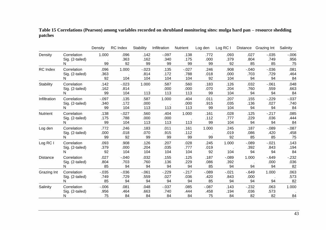
Table 15 Correlations (Pearson) among variables recorded on shrubland monitoring sites: mulga hard pan – resource shedding
patches
Density RC Index Stability Infiltration Nutrient Log den Log RC I Distance Grazing Int Salinity
Density Correlation 1.000 .096 .142 -.097 .138 .772 .093 .027 -.035 -.006 Sig. (2-tailed) . .363 .162 .340 .175 .000 .379 .804 .749 .956 N 99 92 99 99 99 99 92 85 85 75
RC Index Correlation .096 1.000 -.023 .135 -.027 .246 .908 -.040 -.036 .081 Sig. (2-tailed) .363 . .814 .172 .788 .018 .000 .703 .729 .464 N 92 104 104 104 104 92 104 94 94 84
Stability Correlation .142 -.023 1.000 .587 .560 .183 .126 .032 -.061 .048 Sig. (2-tailed) .162 .814 . .000 .000 .070 .204 .760 .559 .663 N 99 104 113 113 113 99 104 94 94 84
Infiltration Correlation -.097 .135 .587 1.000 .404 .011 .207 .155 -.229 -.037 Sig. (2-tailed) .340 .172 .000 . .000 .915 .035 .136 .027 .740 N 99 104 113 113 113 99 104 94 94 84
Nutrient Correlation .138 -.027 .560 .404 1.000 .161 .028 .125 -.217 .085 Sig. (2-tailed) .175 .788 .000 .000 . .112 .777 .229 .036 .444 N 99 104 113 113 113 99 104 94 94 84
Log den Correlation .772 .246 .183 .011 .161 1.000 .245 .187 -.089 -.087 Sig. (2-tailed) .000 .018 .070 .915 .112 . .019 .086 .420 .458 N 99 92 99 99 99 99 92 85 85 75
Log RC I Correlation .093 .908 .126 .207 .028 .245 1.000 -.089 -.021 .143 Sig. (2-tailed) .379 .000 .204 .035 .777 .019 . .392 .843 .194 N 92 104 104 104 104 92 104 94 94 84
Distance Correlation .027 -.040 .032 .155 .125 .187 -.089 1.000 -.649 -.232 Sig. (2-tailed) .804 .703 .760 .136 .229 .086 .392 . .000 .036 N 85 94 94 94 94 85 94 94 94 82
Grazing Int Correlation -.035 -.036 -.061 -.229 -.217 -.089 -.021 -.649 1.000 .063 Sig. (2-tailed) .749 .729 .559 .027 .036 .420 .843 .000 . .573 N 85 94 94 94 94 85 94 94 94 82
Salinity Correlation -.006 .081 .048 -.037 .085 -.087 .143 -.232 .063 1.000 Sig. (2-tailed) .956 .464 .663 .740 .444 .458 .194 .036 .573 . N 75 84 84 84 84 75 84 82 82 84
44
Figure 14: Relationships between shrub density and RC Index on shrubland
monitoring sites
Species composition and landscape function
Background
Most studies on effects of species composition on ecosystems function (mostly in
terms of total productivity) have examined the effect of numbers of species rather than
large shifts in structural composition. (These studies have produced conflicting
information.) Our interest is not whether number of species is affecting landscape
function, but whether shifts in structural composition are important (e.g. shifts from
multi-stemmed shrubs to single stemmed shrubs, or from fire sensitive species to fire
tolerant species). It is unlikely that less significant change, for example substitution of
Aristida spp for Astrebla spp, will affect landscape function in any measurable way.

45
Approach
I outline some examples of structural change and the likely impacts on RC index and
Stability rating in Table 16.
Table 16 Examples of structural change in vegetation and likely impacts on
landscape function as indicated by RC index and Stability rating
Structural transition in vegetation
composition
Change in landscape function
RC index Stability rating
Resilient
landscapes
Non-resilient
landscapes
Tussock grassland to annual herb/grass ↓ NC or ↓ ↓
Tussock grassland to tussock grassland
and woody species
NC NC NC
Hummock grassland to shrubland ↓ NC ↓
Shrubland/woodland to annual
herb/grass ↓ NC or ↓ ↓
Annual herb/grass to shrubland
(coarse-scale) – non-resilient landscape ↑ NC ↑
Annual herb/grass to annual herb/grass
– resilient landscape
NC NC NC
NC: no change
Table 16 may be used as a provisional framework for interpreting change in species
composition and trends in landscape function. In many cases these major shifts in
structural composition are associated with a change in the RC index. Regional scale
reporting should focus on these major shifts.
Relationships between reporting of landscape function and reporting for pastoral production
Earlier I showed that there was a reasonable relationship between shrub/tree density
and landscape function, but an ambiguous relationship with perennial grass frequency.
In reporting change on monitoring sites it is important to firstly establish if the
physical or geo-physical capacity of the landscape to support and produce vegetation
has been altered (i.e. change in landscape function) and then secondly, to assess
change in the biological capacity of the landscape to support the selected land use
(plant species composition and abundance are the important biological characteristics
for pastoral land use). Thus two simultaneous sets of data are required to report
change for pastoral purposes, one set dealing with landscape function and the other
with vegetation change. While some inferences may be made between these data sets,
as shown above, generally these two data sets should be treated and assessed
independently. I see little purpose at this stage in mounting a major research program
to investigate relationships between species composition and landscape function.

46
While these data sets are assessed independently, they should be reported
simultaneously to provide a complete overview. I have outlined a simple approach to
scoring change in species density and composition from a pastoral perspective and
included this in the pro-forma for reporting change on each southern monitoring site
(Appendix 2). A similar approach could be used for reporting change in frequency of
perennial grasses.
Table 17: Suggested ratings for pastoral land-use for change in density of
‘desirable and ‘undesirable’ perennial shrubs.
Significant change*
Desirables Undesirables Rating Display code
↑ ↓ 9 + + +
↑ NC 8 + + +
↑ ↑ ∆ D > ∆ U 7 + +
NC ↓ 6 +
NC NC 5 0
↑ ↑ ∆ D ≤ ∆ U 4 —
NC ↑ 3 — —
↓ NC 2 — —
↓ ↑ 1 — — —
Change deemed ‘significant’ if the following ‘rules’ are met:
Number of desirable or undesirable
plants on the site
Change from assessment 1 to assessment 2
%
> 50 > 10
> 20 – 50 > 20
10 ≥ 20 > 50
< 10 NS
MS Access tables:alec_function_dens_change_9500; alec_density_w_DIU_ass1_ass2;
DES_INDEX.

47
References
Friedel, M.F. (1991). Range condition assessment and concept of thresholds: A
viewpoint. Journal of Range Management 44: 422-426.
Holm, A.M., Bennett, L.T., Loneragan, W.A., and Adams, M.A. (2001). Relationships
between empirical and nominal indices of landscape function in the arid
shrubland of Western Australia. Journal of Arid Environments. (In press)
SPSS Inc (1999) SPSS Base 9.0. Applications Guide SPSS Marketing Department,
Chicago Illinois. 412 pp.
Tongway, D. (1994) Rangeland soil condition assessment manual C.S.I.R.O.
Publications, Canberra. Australia. 69 pp.
Tongway, D. and Hindley, N. (1995) Manual for Soil Condition Assessment of
Tropical Grasslands CS.I.R.O. Australia, Canberra. 60 pp.
Tongway, D.J. and Hindley, N. (2000). Ecosystem function analysis of rangeland
monitoring data - Rangelands Audit Project 1.1. National Land and Water
Resources Audit, Canberra ACT. 35 pp
48
Appendices
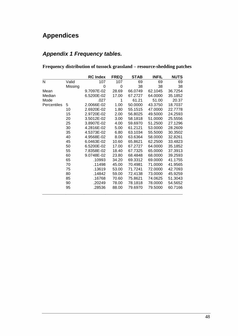
Appendix 1 Frequency tables.
Frequency distribution of tussock grassland – resource-shedding patches
RC Index FREQ STAB INFIL NUTS
N Valid 107 107 69 69 69 Missing 0 0 38 38 38 Mean 9.7097E-02 28.69 66.0749 62.1045 36.7254 Median 6.5200E-02 17.00 67.2727 64.0000 35.1852 Mode .027 1 61.21 51.00 20.37 Percentiles 5 2.0066E-02 1.00 50.0000 43.3750 18.7037 10 2.6920E-02 1.80 55.1515 47.0000 22.7778 15 2.9720E-02 2.00 56.8025 49.5000 24.2593 20 3.5012E-02 3.00 58.1818 51.0000 25.5556 25 3.8907E-02 4.00 59.6970 51.2500 27.1296 30 4.2816E-02 5.00 61.2121 53.0000 28.2609 35 4.5373E-02 6.80 63.1034 55.5000 30.3502 40 4.9568E-02 8.00 63.6364 58.0000 32.8261 45 6.0463E-02 10.60 65.8621 62.2500 33.4823 50 6.5200E-02 17.00 67.2727 64.0000 35.1852 55 7.8358E-02 18.40 67.7325 65.0000 37.3913 60 9.0748E-02 23.80 68.4848 68.0000 39.2593 65 .10993 34.20 69.3312 69.0000 41.1755 70 .11498 45.00 70.4981 71.0000 41.9565 75 .13619 53.00 71.7241 72.0000 42.7093 80 .14842 59.00 72.4138 73.0000 45.9259 85 .16768 70.60 75.8621 74.0625 51.3043 90 .20249 78.00 78.1818 78.0000 54.5652 95 .28536 88.00 79.6970 79.5000 60.7166

49
Frequency distributions of hummock grassland – resource-shedding patches
RC Index FREQ STAB INFIL NUTS
N Valid 36 37 27 27 27 Missing 1 0 10 10 10 Mean .16464 12.76 58.0560 51.6831 29.0874 Median .15044 5.00 57.3574 51.5000 26.2963 Mode .205 1 53.51 44.00 18.70 Percentiles 5 1.5053E-02 1.00 45.1400 37.0000 17.2593 10 2.8450E-02 1.00 46.9189 40.4444 18.5926 15 3.9447E-02 1.00 48.8108 42.4000 18.7407 20 5.7017E-02 2.00 50.5946 44.0000 19.2222 25 6.3841E-02 2.00 52.9730 46.0000 19.6296 30 7.4991E-02 2.40 53.5135 46.4000 21.2778 35 9.0469E-02 3.00 54.3784 47.0000 22.8148 40 .11079 4.00 55.1351 47.6000 23.6296 45 .12801 4.10 57.2973 48.6000 24.8519 50 .15044 5.00 57.3574 51.5000 26.2963 55 .16877 6.00 57.8378 53.3556 28.1111 60 .17817 6.80 59.5676 53.9778 29.6667 65 .20540 7.00 60.7371 55.2000 32.4239 70 .22267 8.00 61.9590 56.6000 33.2922 75 .23768 9.50 63.0303 58.0000 37.0370 80 .25174 11.20 63.2727 58.4000 38.8889 85 .27825 22.50 67.2727 60.6000 42.1852 90 .32022 45.80 69.7756 65.6000 45.4074 95 .48960 78.10 76.8485 69.2000 51.6296

50
Frequency distributions of sandplain – site-scale
RC Index STAB INFIL NUTS
N Valid 35 33 33 33 Missing 0 2 2 2 Mean .1887 60.01 50.56 33.58 Median .1610 61.63 50.81 34.90 Mode .05 49 34 19 Percentiles 5 4.610E-02 49.69 37.63 19.73 10 5.630E-02 52.62 44.87 22.02 15 6.815E-02 53.94 45.86 23.65 20 8.280E-02 54.64 47.12 26.22 25 9.500E-02 54.95 47.60 26.84 30 .1028 55.84 47.94 28.81 35 .1124 56.53 48.38 31.69 40 .1404 57.28 49.05 33.07 45 .1530 59.29 49.66 34.61 50 .1610 61.63 50.81 34.90 55 .1698 61.97 52.32 36.10 60 .1868 62.85 52.82 37.19 65 .2100 63.01 53.10 38.47 70 .2310 63.91 53.38 39.04 75 .2650 64.28 53.55 39.82 80 .3072 65.58 54.45 39.87 85 .3222 66.08 55.58 40.09 90 .3698 68.16 57.12 42.88 95 .4736 69.03 60.14 44.28

51
Frequency distributions of shrub-steppe sites – site-scale
RC Index STAB INFIL NUTS
N Valid 593 552 552 552 Missing 0 41 41 41 Mean .1272 62.60 48.68 35.75 Median .1040 63.25 48.14 35.83 Mode .09 66 24 14 Percentiles 5 3.035E-02 51.07 37.65 23.39 10 4.070E-02 53.54 40.03 25.76 15 5.010E-02 55.54 41.29 27.57 20 5.790E-02 57.49 42.15 29.15 25 6.450E-02 58.46 43.31 30.86 30 7.200E-02 59.64 44.48 31.78 35 8.245E-02 60.84 45.09 32.80 40 8.800E-02 61.60 46.14 33.54 45 9.500E-02 62.50 47.27 34.48 50 .1040 63.25 48.14 35.83 55 .1154 64.01 48.83 36.71 60 .1250 64.55 50.27 37.62 65 .1380 65.18 51.55 38.54 70 .1509 66.20 52.36 39.46 75 .1680 66.88 53.33 40.69 80 .1842 67.86 54.56 41.95 85 .2120 68.86 55.69 43.90 90 .2413 70.59 57.88 46.09 95 .3137 72.60 61.37 48.81

52
Frequency distributions of mulga-hardpan – site-scale
RC index STAB INFIL NUTS
N Valid 35 33 33 33 Missing 0 2 2 2 Mean .1887 60.01 50.56 33.58 Median .1610 61.63 50.81 34.90 Mode .05 49 34 19 Percentiles 5 4.610E-02 49.69 37.63 19.73 10 5.630E-02 52.62 44.87 22.02 15 6.815E-02 53.94 45.86 23.65 20 8.280E-02 54.64 47.12 26.22 25 9.500E-02 54.95 47.60 26.84 30 .1028 55.84 47.94 28.81 35 .1124 56.53 48.38 31.69 40 .1404 57.28 49.05 33.07 45 .1530 59.29 49.66 34.61 50 .1610 61.63 50.81 34.90 55 .1698 61.97 52.32 36.10 60 .1868 62.85 52.82 37.19 65 .2100 63.01 53.10 38.47 70 .2310 63.91 53.38 39.04 75 .2650 64.28 53.55 39.82 80 .3072 65.58 54.45 39.87 85 .3222 66.08 55.58 40.09 90 .3698 68.16 57.12 42.88 95 .4736 69.03 60.14 44.28

53
Frequency distributions – sandplain and mulga hardpan – resource shedding
patches RC Index Density Stability Infiltration Nutrient
N Valid 140 145 158 158 158 Missing 18 13 0 0 0 Mean .20785 3551.00 60.9923 47.6977 30.7465 Median .16950 2533.33 60.9029 46.7244 30.2662 Mode .110 2233 67.57 41.83 21.16 Percentiles 5 5.0500E-02 664.58 50.0775 38.9551 18.8746 10 7.0000E-02 966.67 53.2987 41.3553 21.0229 15 8.0500E-02 1197.02 54.4125 41.8944 22.8086 20 9.4000E-02 1358.33 55.4366 42.7742 24.1906 25 .10425 1558.33 56.3707 43.4066 25.3086 30 .11250 1858.33 57.4797 43.8884 25.6314 35 .12815 2104.17 58.5515 44.4542 26.2917 40 .14075 2225.00 59.4775 45.3967 27.3364 45 .15625 2391.67 60.2989 46.1538 28.4259 50 .16950 2533.33 60.9029 46.7244 30.2662 55 .19733 2783.33 62.0606 47.7104 31.2091 60 .20600 3166.67 62.6006 48.3547 32.8796 65 .21875 3361.11 63.3604 49.7285 33.9142 70 .24611 3633.33 64.0631 50.5800 34.4481 75 .26600 4300.00 64.9149 52.0243 35.4167 80 .27800 4766.67 66.2072 52.5821 36.9907 85 .31730 5450.00 67.4903 53.3260 38.6185 90 .43320 6733.33 69.0811 55.2163 40.1663 95 .54000 8616.67 70.8340 58.2218 43.9373
a Calculated from grouped data. b Multiple modes exist. The smallest value is shown c Percentiles are calculated from grouped data.
54
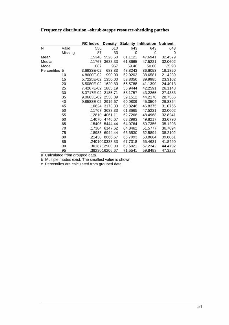
Frequency distribution –shrub-steppe resource-shedding patches
RC Index Density Stability Infiltration Nutrient
N Valid 556 610 643 643 643 Missing 87 33 0 0 0 Mean .15340 5526.50 61.1121 47.6941 32.4579 Median .11767 3633.33 61.8665 47.5221 32.0602 Mode .087 967 59.46 50.00 25.93 Percentiles 5 3.6933E-02 683.33 48.8243 36.6053 19.1850 10 4.8600E-02 990.00 52.0202 38.6581 21.4239 15 5.7225E-02 1350.00 53.8056 39.9985 23.3102 20 6.5080E-02 1620.83 55.5788 41.1390 24.4013 25 7.4267E-02 1885.19 56.9444 42.2591 26.1148 30 8.3717E-02 2185.71 58.1757 43.2265 27.4383 35 9.0663E-02 2538.89 59.1512 44.2178 28.7556 40 9.8588E-02 2916.67 60.0809 45.3504 29.8854 45 .10824 3173.33 60.8246 46.8375 31.0766 50 .11767 3633.33 61.8665 47.5221 32.0602 55 .12810 4061.11 62.7266 48.4968 32.8241 60 .14070 4746.67 63.2993 49.8217 33.6790 65 .15406 5444.44 64.0764 50.7356 35.1293 70 .17304 6147.62 64.8462 51.5777 36.7894 75 .18988 6944.44 65.6530 52.5894 38.2102 80 .21430 8666.67 66.7093 53.8684 39.8061 85 .24010 10333.33 67.7318 55.4631 41.8490 90 .30187 12900.00 69.6021 57.2342 44.4792 95 .38230 16206.67 71.5541 59.8483 47.3287
a Calculated from grouped data. b Multiple modes exist. The smallest value is shown c Percentiles are calculated from grouped data.

55
Appendix 2: Examples of presentations of landscape function at the site scale

56
Functional type: Sandplain community
Percentile RC Index Stability Infiltration Nutrient Density Site ranking: WEE 001
Ratings
N 288 354 354 354 318 RC Index Stability Infiltration Nutrient Plant density
1995 2000 1995 2000 1995 2000 1995 2000 1995 2000
95 0.541 76.8 65.4 51.0 8577
90 0.428 73.8 62.1 47.7 6733
85 0.318 71.6 59.6 45.1 5467
80 0.276 69.8 58.2 43.5 4815
75 0.266 68.9 56.7 41.5 4358
70 0.245 67.6 55.8 39.8 3783
65 0.218 66.9 54.3 38.0 3433
60 0.205 65.5 53.3 36.2 3200
55 0.197 64.6 52.6 34.8 2858
50 0.169 63.5 51.8 33.3 2625
45 0.156 62.7 50.5 31.5 2467
40 0.140 62.2 49.4 30.6 2253
35 0.123 61.4 48.1 28.9 2127
30 0.112 60.2 46.8 27.5 1933
25 0.102 58.8 45.9 26.0 1625
20 0.093 57.8 44.2 25.2 1383
15 0.079 56.3 43.2 23.7 1217
10 0.068 54.6 41.8 21.3 967
5 0.050 52.4 38.7 18.1 666
Black to black = no significant change; to green positive change;
to red negative change
Pastoral change rating: 0 (ie no change in long-term pastoral value derived from perennial shrubs)
Dysfu
nction
al
F
unctiona
l

57
Functional type: Shrubland (chenopod)
Percentile RC Index Stability Infiltration Nutrient Density Site ranking: RIV 010
Ratings
N 1162 1430 1430 1430 1352 RC Index Stability Infiltration Nutrient Plant density
1995 1999 1995 1999 1995 1999 1995 1999 1995 1999
95 0.384 75.9 66.4 53.9 16058
90 0.300 73.7 63.5 49.6 12667
85 0.239 72.1 61.5 47.2 9894
80 0.213 70.8 59.2 45.4 8100
75 0.187 69.8 57.7 43.5 6733
70 0.171 68.9 56.4 41.7 6063
65 0.153 67.6 55.4 40.1 5235
60 0.140 66.8 53.8 38.4 4609
55 0.127 65.9 53.1 36.9 4000
50 0.116 64.9 51.8 35.5 3533
45 0.107 63.8 51.0 34.0 3067
40 0.097 62.9 50.0 32.7 2785
35 0.088 62.0 48.7 31.3 2383
30 0.081 60.8 47.5 29.8 2098
25 0.072 59.6 46.2 28.0 1817
20 0.063 58.5 44.6 26.2 1567
15 0.055 56.8 43.0 24.1 1267
10 0.045 54.4 40.9 22.2 967
5 0.034 51.2 38.3 19.8 650
Black to black = no significant change; to green positive change; to red negative change
Pastoral change rating: +ve +ve (I.e. significant increase in pastoral value derived from perennial shrubs)
Dysfu
nction
al
F
unctio
nal
