development of ice particle formation system for ice jet ... · technology (crc-imst) for...

Development of Ice Particle

Production System for Ice Jet Process

Dinesh Kumar Shanmugam

A thesis submitted in fulfilment of the requirements for the degree of

Doctor of Philosophy

Industrial Research Institute Swinburne, Faculty of Engineering and Industrial Sciences,

Swinburne University of Technology

June, 2005

Abstract

This thesis presents a comprehensive study of the ice particle production process through

experimentation and numerical methods using computational fluid dynamics (CFD) that

can be used to produce ice particles with controlled temperature and hardness for use in ice

jet (IJ) process for industrial applications. The analytical and numerical modeling for the

heat exchanger system are developed that could predict the heat, mass and momentum

exchange between the cold gas and water droplets. Further, the feasibility study of the

deployment of ice particles produced from the ice jet system for possible cleaning and

blasting applications are analyzed numerically.

Although the use of Abrasive Water Jet (AWJ) technology in cutting, cleaning, machining

and surface processing is a very successful industrial process, a considerable amount of

secondary particle waste and contamination impingement by abrasive materials has been an

important issue in AWJ process. Some alternate cryogenic jet methods involving vanishing

abrasive materials, such as plain liquid nitrogen or carbon dioxide have been tried for these

applications, but they also suffer from certain drawbacks relating to the quality, safety,

process control and materials handling.

The use of ice jet process involving minute ice particles has received relatively little

attention in industrial applications. Some researches have concentrated on the studies of

effects of Ice Jet outlet parameters of the nozzle and focus tube for machining soft and

brittle materials. Most of the work in this area is qualitative and researchers have paid a

cursory attention to the ice particles temperature and the efficiency of production of these

particles. An extensive investigation to gain insight knowledge into the formulation of ice

formation process parameters is required in arriving at a deeper understanding of the entire

ice jet process for production application.

Experimental investigations were focussed on the measurement of ice particle temperature,

phase transitions, ice particle diameter, coalescence and hardness test. The change in ice

particle diameter from the inlet conditions to the exit point of the heat exchanger was

i

investigated using the experimental results. These observations were extended to numerical

analysis of temperature variations of ice particles at different planes inside the custom built

heat exchanger. The numerical predictions were carried out with the aid of visualization

studies and temperature measurement results from experiments. The numerical models

were further analysed to find out the behaviour of ice particles in the transportation stage,

the mixing chamber of the nozzle and focus tube. This was done to find out whether the

methodology used in this research is feasible and if it can be used in applications such as

cleaning, blasting, drilling and perhaps cutting.

The results of the empirical studies show that ice particles of desired temperature and

hardness could be produced successfully with the current novel design of the heat

exchanger. At the optimum parameters, ice particles could be produced below -60°C, with

hardness of particles comparable to gypsum (Moh’s hardness of 1.5 to 3). The visualization

studies of the process assisted in observation of the phases of ice at various points along the

heat exchanger. The results of numerical analysis were found to agree well with the

experiments and were supported by the statistical model assessments. Numerical analyses

also show the survival of ice particles at the nozzle exit even with high-pressure, high-

velocity water/air mixture.

ii

Acknowledgements I would like to thank my academic supervisors Professor Syed Masood and

Professor Milan Brandt for their crucial support and guidelines, encouragement

and helpful disposition and other general assistance during my research work at

the Industrial Research Institute Swinburne (IRIS), Faculty of Engineering and

Industrial Sciences, Swinburne University of Technology. I would also like to

thank Cooperate Research Centre for Intelligent Manufacturing Systems and

Technology (CRC-IMST) for supporting this project.

In addition, I would like to extend my sincere gratitude to Professor E. Siores, Dr F.

Chen, Professor Yos Morsi and Drs. Rowan Deam and Engida Lemma for their

expert guidance and timely assistances during the course of this research. I would

like to thank A.F.K Engineering and British Oxygen Company (BOC) for their

assistance in conducting experiments. Finally, I would like to thank my family for

their support and encouragement throughout my research.

iii

Declarations This thesis contains no material which has been accepted for the award

of any other degree or diploma, except where due reference is made in

the text of the thesis. To the best of my knowledge, this thesis contains

no material previously published or written by another person except

where due reference is made in the text of the thesis

Signed …………………………………..

Dinesh Kumar Shanmugam Dated ………………..............................

iv

List of Publications D. K. Shanmugam, F. L. Chen, “Comparative study of Jetting Machining Technologies

over Laser Machining Technology for cutting Composite Materials”, Journal of Composite

Structures, 2002, vol. 57/1-4 pp. 289-296.

D.K Shanmugam, Y. Morsi, “Study of Ice Particle Production Using Experimental and

Computational Fluid Dynamic Methods”, 2003 WJTA American Waterjet Conference, 17-

19 August 2003, Houston, Texas.

D.K Shanmugam, F.L. Chen, “Development of Cryogenic Ice Jet technology”, Seventh

International Conference on Manufacturing & Management PCM’2002, 27-29 November

2002, Bangkok, Thailand, pp. 574-579.

D.K Shanmugam, F.L. Chen, “Study of Ice Particle Formation Process, Proceedings of the

Fourth International Conference on Modeling and Simulation”, 11-13 November, 2002,

Melbourne, Australia, pp. 323-327.

v

Table of Contents Abstract i Acknowledgements iii Declarations iv List of Publications v Table of Contents vi Lists of Figures xii Lists of Tables xx Nomenclature xxii Chapter 1 Introduction 1.1 Background 1 1.2 Working principle of Ice Jet 3 1.3 Objective and Scope of the Project 5 1.4 Organization of Research Work 6 1.5 Outline of Chapters 7 Chapter 2 Literature review 2.1 Overview of the Review Process 9 2.2 Various Jetting and Blasting Processes 9

2.2.1 Development of WJ and AWJ Processes 9 2.2.2. Cryogenic Jets 12

2.2.2.1 CO2 Jet 12 2.2.2.2 Liquid Nitrogen Jet 14 2.2.2.3 Liquid Ammonia Jet 16 2.2.2.4 Cryogenic Abrasive Jet 16

2.3 Development of Ice Jet Technology 17 2.3.1Air Ice Jet 20 2.3.2Water Ice Jet 21

2.4 Applications of Ice jet 22 2.4.1 Ice Jet Cleaning 22 2.4.2 Ice Jet for Machining 24 2.4.3 Biomaterial 26 2.4.4 Nuclear 26 2.4.5 Potential Application in Surgery 26

vi

2.4.6 Numerical Modeling of Ice Jet 27 2.5 Spray Crystallization 30 2.6 Numerical Simulations of Phase Change Problems 32 2.7 Visualization Studies 34 2.8 Refrigeration 36 2.9 Ice Aerosol Modeling 36 2.10 Physics of Water Ice 37

2.10.1 Adhesion 40 2.10.2 Sintering 41 2.10.3 Shear Strength 42 2.10.4 Granulometric Composition as a function of Ice Temperature 43 2.10.5 Density 44 2.10.6 Coefficient of Linear Expansion 45 2.10.7 Poisson’s Ratio 45 2.10.8 Thermal Conductivity 46 2.10.9 Tensile Yield Strength 47

2.11 Summary 48

Chapter 3 Design and Development of Ice Jet System 3.1 Introduction 49 3.2 Selection of Atomizer 49

3.2.1 Water Sprayer 50 3.2.2 Pneumatic Atomizer 51 3.2.3 Ultrasonic Atomizer 52 3.2.4 Calibration of droplet size 53 3.2.5 Operating principle of PDPA 53 3.2.6 Selection of Atomizer probe 54

3.3 Design of Heat Exchanger 55 3.3.1 Lumped capacitance method 56 3.3.2 Heat Exchanger diameter 57

3.4 Design of Ice Slurry Transportation System 63 3.5 Design of Ice Jet Cleaning Nozzle 64 Chapter 4 Experimental Setup and Procedure 4.1 Overview 66 4.2 Ice Particle formation process 66 4.3 Measuring Devices and Accuracy Assessment 68

vii

4.3.1 Thermocouple 68 4.3.2 Cryogenic Nitrogen Mass Flow Rate Measurements 69 4.3.3 Water Flow meter 69 4.3.4 Inlet Tube Angle of Nitrogen 69 4.4 Design of Experiments 70 4.5 Visualization Experiments 71 Chapter 5 Modeling of Ice Jet Process 5.1 Introduction 75 5.2 Problem Definition in Modeling 75

5.2.1 Heat Transfer inside Heat Exchanger 76 5.2.2 Ice Slurry Transportation System 78 5.2.3 Ice Jet Nozzle 79

5.3 Hypothesis 79 5.4 Governing Equations 80

5.4.1 Interfacial Area Density 80 5.4.1.1 Particle Model 81

5.4.2 Inter-Phase Heat Transfer 81 5.4.2.1 Particle Model Correlations 83 5.4.2.2 Interface Flux 84

5.4.3 Thermal Phase Change 84 5.4.3.1 Latent Heat 85 5.4.3.2 The Two Resistance Model 85 5.4.3.3 Secondary Fluxes 86

5.4.4 Inter-Phase Mass Transfer 87 5.4.5. Inter-Phase Momentum Transfer Models 88

5.4.5.1 Inter-Phase Drag 89 5.4.5.2 Inter-Phase Drag for the Particle Model 90

5.4.6 Turbulent Modeling in Multiphase Flow 93 5.4.6.1 Phase-Dependent Turbulence Models 93

5.5 Discretization of the Governing Equations 94 5.5.1 Transient Term 96 5.5.2 Diffusion Term 96 5.5.3 Advection Term 97

5.6 Solution Method 97 5.7 Algebraic Multigrid 98

viii

Chapter 6 Experimental Investigation of Ice Particles Formation Process 6.1 Introduction 100 6.2 Temperature Measurements (Time Dependant) 100

6.2.1 Calculation of Heat Loss 101 6.2.2 Initial Temperature Measurements along the Heat-Exchanger 102 6.2.3 Effect of Cryogenic Nitrogen Inlet Temperature 105 6.2.4 Effect of Inlet Flow Rate of Cryogenic Nitrogen 106 6.2.5 Effect of Inlet Cryogenic Nitrogen Entry angle 107 6.2.6 Effect of Inlet Water Temperature 109 6.2.7 Effect of Inlet Water Flow Rate 111 6.2.8 Effect of Initial Droplet Diameter 112 6.2.9 Effect of Inlet Air Temperature 113 6.2.10 Effect of Air Flow Rate 115 6.2.11 Temperature Curves of Nitrogen 116 6.2.12 Wall Temperature Curves 117

6.3 Effect of Cryogenic Nitrogen Inlet Temperature (Time dependent) 121 6.4 Visualization Experiment for Droplet Diameter 121

6.4.1 Initial Droplet Diameter versus Outlet Ice Particle Diameter 122 6.4.2 Different Phases of Water /Ice Using Image Polarization Technique 123 6.4.3 Coalescence 127

6.5 Measurement of Hardness 129 6.6 Summary 131 Chapter 7 Numerical Modeling of Ice Particle Formation and Ice Jet Process 7.1 Introduction 132 7.2 Structure of CFX 132 7.3 Boundary Conditions 134 7.4 Grid Independence Test 135 7.5 Temperature Distribution Study 139

7.5.1 Visualization at Different Planes 139 7.5.2 Outlet Temperature Distribution of Cryogenic Nitrogen 149 7.5.3 Air Temperature at the Outlet 151

7.6 Temperature Plots 152 7.6.1 Ice Particle Distribution 152 7.6.2 Temperature Variation Study 153 7.6.3 Air Temperature 155

7.7 Volume Fraction 156

ix

7.8 Velocity Vectors 159 7.9 Particle Trajectory of Water 165 7.10 Model Assessment 168 7.11 Extrapolation of Numerical Model 174 7.12 Ice Slurry Transportation System 175 7.13 Ice jet 181

7.13.1 Boundary Conditions 182 7.13.2 Grid Independence Test 183 7.13.3 Air Ice Jet 184 7.13.4 Water Ice Jet Simulations 188 7.13.5 Velocity Distribution 191 7.13.6 Pressure Distribution 192

7.14 Conclusions 194 Chapter 8 Conclusions and Recommendations 8.1 Introduction 195 8.2 Experimental Study of Temperature Measurements 195 8.3 Visualization Study 196 8.4 Numerical Modeling Study of Ice Particle Formation 197 8.5 Numerical Modeling of Ice Transportation and Ice Jet 198 8.6 Recommendations for follow-up work 199 References 200 Appendix A Basic Definitions

A1 Multiphase Flow 211

A2 Dispersed Phase 212

A3 Volume Fraction 213

A4 Control Volume of Single Droplet 213

A5 Turbulent Modeling in Multiphase Flow 214

A6 Coordinate System 215

Appendix B B1 Cross Section of the Heat Exchanger 216

B2 Exploded View of Air Inlet System 217

x

B3 Top Portion 218

B4 I-Insert 219

B5 II-Insert 220

B6 Air Supply Chamber 221

Appendix C Sample CFX program 222

xi

List of Tables Table 3.1 Material properties of Aluminum 60

Table 3.2 Thermal properties of Aluminum 61

Table 4.1 Initial Range of Experimental Parameters 70

Table 4.2 Range of Parameters for Visualization Experiments 72

Table 6.1 Parameters Considered for Ice Particle Temperature along the Heat-Exchanger

103


105

Table 6.3 Parameters Considered for the Range of Cryogenic Nitrogen Flow Rate 106

Table 6.4 Parameters Considered for Inlet Nitrogen Angle 108

Table 6.5 Parameters Considered for Inlet Water Temperature 110

Table 6.6 Parameters Considered for Water Flow Rate 111

Table 6.7 Parameters Considered for Initial Droplet Diameter 112

Table 6.8 Parameters Considered for the Range of Air Temperature 114

Table 6.9 Parameters Considered for the Range of Air Flow Rate 115

Table 6.10 Parameters Considered for Wall Temperature Measurements along the Surface of the Heat Exchanger

118

Table 6.11 Tabulation of T Difference-Ice for Nitrogen Flow Rate of 0.5 l/min 120



Table 6.14 Parameters Considered for Polarization Technique 124

Table 6.15 Parameters Considered for Measuring Coagulated Particle Diameter 128

Table 6.16 Parameters for Brinell Hardness Test for Ice 129

Table 7.1 Boundary Conditions at Inlet and Outlet 135

Table 7.2 Number of Grids on Each Axis for the Heat Exchanger 136

Table 7.3 Physical Properties of Water and Nitrogen for Numerical Predictions 138


139

xx

Table 7.5 Classification of Parameters 140

Table 7.6 Interpretation of Phase in Terms of Temperature 172

Table 7.7 Boundary Conditions for a) Inlet and b) Outlet of Ice Slurry Transfer System

175 176

Table 7.8 Initial Conditions of Inlet1 and Inlet2 of Ice Jet Nozzle 182

Table 7.9 Number of Grids on Each Axis for the Nozzle 184

xxi

List of Figures

Figure 1.1 Mechanisms of Material-Removal by Solid-Particle Erosion 2

Figure 2.1 OMAX 2652p Pictured with Automatic Z-axis 11

Figure 2.2 State diagram of Carbon dioxide 13

Figure 2.3 Dry Ice Blasting (Courtesy Cold Jet Inc.) 13

Figure 2.4 Schematic of Ultra High Pressure Liquid Nitrogen Jet 15

Figure 2.5 Schematic of Ice Jet System for Drilling 25

Figure 2.6 Phase Diagram of Water-Ice 38

Figure 2.7 Strength of Adhesion of Ice Particles 41

Figure 2.8 Schematic of the Sintering of Ice Particles 41

Figure 2.9 Shear Strength of Ice Adhesion to Stainless Steel 42

Figure 2.10 Force Required to Separate Two Spheres at Ice Saturation against Temperature

43

Figure 2.11 Density of T-1 Ice Type as a Function of Temperature at Atmospheric Pressure

44

Figure 2.12 Coefficient of Linear Expansion of T-1 Type Polycrystalline Ice at Atmospheric Pressure According to Jacob and Erk

45

Figure 2.13 Poisson’s Ratio of the Polycrystalline Ice as a Function of Temperature

46

Figure 2.14 Thermal Conductivity of Polycrystalline Ice as a Function of Temperature According to Ratcliffe

47

Figure 2.15 Tensile Strength of Polycrystalline Ice as a Function of Temperature [Butkovich]

48

Figure 3.1 Front View of the Sprayer 51

Figure 3.2 Schematic Depiction of Pneumatic Atomizer 52

Figure 3.3 Ultrasonic Atomizer Model VC 130 AT with Flat Probe 53

Figure 3.4 Operating Principle of PDPA 54

Figure 3.5 a) Flat Tip Half Wave Medium Atomization Rate (200ml/min)

b) Flat Tip Half wave Low Atomization Rate (60ml/min)

55

xii

Figure 3.6 Flat Probe Atomizing the Water Droplets 55

Figure 3.7 a) Water Flow Rate of 1 l/hr at the Amplitude of 40

b) Water Flow Rate of 6 l/hr at the Amplitude of 80

58

Figure 3.8 a) Showing Water Flow Rate of 12 l/hr and Amplitude of 100,

b) Shows an Equalized Contract of the Atomized Water Droplets Pattern.

58

Figure 3.9 Illustration of the Discharge Angle, the Discharge Diameter and the Atomized Droplets (Φ = Curvature expressing the energy loss of the atomized water droplets, θ = discharged angle, Rd = discharge radius)

59

Figure 3.10 3-D Shell Model of the Heat Exchanger Showing Finite Elements 60

Figure 3.11 Temperature Distribution of Heat Exchanger 62

Figure 3.12 Displacement-Magnitude of the Heat Exchanger 62

Figure 3.13 Stress-Strain Distribution of the Heat Exchanger 63

Figure 3.14 a) and b) Shows the Start and End Section of the Ice Slurry Transport System in 3-D Model with the Datum Planes

64

Figure 3.15 Design of Ice Jet Nozzle With the Focus Tube 65

Figure 4.1 Schematic of the Ice Slurry Formation Process and Temperature Measurement System

67

Figure 4.2 Schematic of the Ice Slurry Formation Process with Camera Attached for Visualization Study

71

Figure 4.3 PULNIX TM-6710 High Resolution Progressive Scan Camera Used in the Visualization Experiments

72

Figure 4.4 Attachments and Accessories of the Ice Jet System 73

Figure 5.1 Droplets Dispersed by an Atomizer with Cryogenic Nitrogen Gas Flowing Over it.

76

Figure 5.2 Introduction of Air Inlet System on the Lower Block of the Heat Exchanger

77

Figure 5.3 Schematic of the Representation of Transportation System 78

Figure 5.4 Representation of Different Inlet and Phase Inside the Nozzle. 79

Figure 5.5 Finite Volume Surface 95

Figure 5.6 Solution Procedure for the Discretized Equations 99

xiii

Figure 6.1 Temperature Curves Measured at Inlet and Exit Point of the Heat Exchanger for the Transfer Tube Length of 1m

101

Figure 6.2 Temperature Curves Measured at Inlet and Exit Point of the Heat Exchanger for the Transfer Tube Length of 1.6m

101

Figure 6.3 Positions of Thermocouples along Heat Exchanger 103

Figure 6.4 Measure of Temperatures at Different Points of the Heat Exchanger for Parameters Shown in Table 6.2

104

Figure 6.5 Time Plot of Ice Particle temperature by Decreasing Inlet Nitrogen Temperature to -100°C and -120°C for the Parameters Shown in Table 6.3

106

Figure 6.6 Time Plot of Ice Particle Temperatures as a Function of Nitrogen Flow Rate

107

Figure 6.7 a) Shows the Angle Without the Offset b) Shows the Angle with the Offset

108

Figure 6.8 Plot of Ice Particle Temperature as a Function of Inlet Nitrogen Angle

109

Figure 6.9 Ice Particle Temperatures for Different Inlet Water Temperature of 5°C, 10°C 15°C for Parameters Shown in Table 6.6

110

Figure 6.10 Plot of Ice Particle Temperature as a Function of Inlet Water Flow Rate

111

Figure 6.11 Ice Particle Temperature for Different Droplet Diameter of 80µm, 100µm and 120µm for the Parameters Shown in Table 6.8

113

Figure 6.12 Plot of Ice Particle Temperature as a Function of Air Temperature 114

Figure 6.13 Plot of Ice Particle Temperature as a Function of Airflow Rate 116

Figure 6.14 Temperature Difference as a Function of Inlet Water Temperature for Inlet Nitrogen Temperature of -120°C

117

Figure 6.15 Temperature Difference as a Function of Inlet Water Temperature for Inlet Nitrogen Temperature of -100°C

117

Figure 6.16 Outer Wall Temperature Measurements 118

Figure 6.17 Plot of Wall Temperature Variations With Time at Four Different Positions as Shown in Figure 6.16 for the Parameters in Table 6.10

119

Figure 6.18 Plot of Ice Particle Temperature with Constant Nitrogen Temperature

121

Figure 6.19 Plot of Mean Diameter of Ice Particles for Nitrogen Temperature of -120°C

123

xiv

Figure 6.20 Plot of Mean Diameter of Ice Particles for Nitrogen Temperature of -100°C

123

Figure 6.21 Image of Falling Particles against a Black Background taken at the Outlet of the Heat Exchanger

124

Figure 6.22 Images of Transition Phases of Water to Ice Particle, a) Dilute Liquid, b) Dense Liquid, c) Dilute Solid and d) Dense Solid

125

Figure 6.23 Particle Distributions against the Polarization at 80mm from the Atomization Position

125

Figure 6.24 Particle Distributions against the Polarization at 200mm from the Atomization Position

126

Figure 6.25 Particle Distributions against the Polarization at the Outlet of the Heat Exchanger

126

Figure 6.26 Images of Falling Ice Particles as Observed for Coalescence 127

Figure 6.27 Plot of Coagulated Particles as a Function of Ice Particle Temperature

128

Figure 6.28 Schematic of the Load Application for Brinell Hardness for Ice 130

Figure 6.29 Brinell Hardness as a Function of Ice Temperature 130

Figure 7.1 Structure of CFX-5.6 133

Figure 7.2 Illustration of Fluid and Solid Boundaries in Heat Exchanger 134

Figure 7.3 Representation of Heat Exchanger Blocks 136

Figure 7.4 Three-Dimensional Grids of Heat Exchanger 137

Figure 7.5 Temperature Distribution of Water Droplets in XY plane for Inlet Condition 1

140


141


141


142


143


143

xv


144


144


146


147


147


148

Figure 7.17 Temperature Distribution of Cryogenic Nitrogen in XY plane at Outlet for Inlet Condition 1

149


150


150

Figure 7.20 Temperature Distribution of Air in XY plane at Outlet for Inlet Condition 1

151

Figure 7.21 Temperature of Ice Particles along the Side walls 152

Figure 7.22 Temperature Variation of Ice Particles along the Vertical axis Excluding the Side walls

152

Figure 7.23 Temperature Variation of Ice Particles and Nitrogen for Inlet Condition 1

153


154


154

Figure 7.26 Air Temperature Variation along the Side walls 155

Figure 7.27 Volume Fraction of Ice Particles on the XY plane at the Outlet of the Heat Exchanger

156

Figure 7.28 Volume Fraction of Cryogenic Nitrogen on the XY plane at the Outlet of the Heat Exchanger

157

xvi

Figure 7.29 Volume Fraction of Different Phases at Nitrogen Flow rate of 0.5 l/min

158


158


158

Figure 7.32 Velocity Vector of Ice Particles a) Top Portion, b) Mid Section and c) Bottom Section of the Heat Exchanger

160

Figure 7.33 Velocity Vector of Nitrogen a) Top Portion and b) Bottom Section of the Heat Exchanger

161

Figure 7.34 Velocity Vector of Air at the Mid Section of the Heat Exchanger 162

Figure 7.35 Velocity Variation of Ice Particles along the Side walls and along the Vertical axis

162

Figure 7.36 Velocity Variation of Cryogenic Nitrogen on the Side walls and along the Vertical axis

163

Figure 7.37 Velocity Variation of air along the side walls and along the vertical axis

164

Figure 7.38 Particle Track of Ice Particles Inside the Heat Exchanger 165

Figure 7.39 Volume Fraction of Ice Particles Impact on Side walls at Increasing Distance

166

Figure 7.40 Streamlines of Cryogenic Nitrogen at a) 1.5 l/min, b) 2.0 l/min and c) 2.5 l/min

167

Figure 7.41 Streamlines of Airflow along the Wall and along the Vertical axis 167

Figure 7.42 Experimental and Simulated Results of Ice Particle Temperature Variations for Varying Cryogenic Nitrogen Temperature

168

Figure 7.43 Experimental and Simulated Results of Ice Particle Temperature Variations for Different Nitrogen Flow Rate

169

Figure 7.44 Experimental and Simulated Results of Ice Particle Temperature Variations for Different Inlet Water Temperature

169

Figure 7.45 Experimental and Simulated Results of Ice Particle Temperature Variations for Constant Cryogenic Nitrogen Temperature

170

Figure 7.46 Frequency Diagram of the Percentage Error between Ice Particle Temperature Difference between Experiments and the Model

171

xvii

Figure 7.47 Best fit of the Ice Particle Temperature Difference between the Experiments and the Model

171

Figure 7.48 Phase Distribution at 80mm from the Inlet Position for Inlet Condition3

172

Figure 7.49 Phase Distribution at 200mm from the Inlet position for Inlet Condition 3

173

Figure 7.50 Phase Distribution at the Outlet for Inlet Condition 3 173

Figure 7.51 Extrapolated Ice Particle Temperature for Cryogenic Nitrogen below Experimental values

174

Figure 7.52 Temperature Distribution Along the Central axis for Inlet Condition 1

176


177


177

Figure 7.55 Temperature Distribution along the Wall for Inlet Condition 1 178



Figure 7.58 Mean Temperature Distribution of Ice Particles Around the Walls and at the Central axis on the XZ plane at the Outlet

180

Figure 7.59 a) Conventional Nozzle used for AWJ in IRIS, b) Modified Nozzle Created for Numerical Ice Jet

182

Figure 7.60 Inlet and Outlet boundaries of the Nozzle 183

Figure 7.61 Three dimensional representations of grids for the nozzle 184

Figure 7.62 Temperature variation along the length of the nozzle 185

Figure 7.63 Temperature variation along the length of the nozzle for air inlet temperature, 10°C

186

Figure 7.64 Temperature variation along the length of the nozzle for different air inlet temperatures

186

Figure 7.65 Temperature distribution a) ice and air on the ice inlet plane, b) cross-sectional view for air

187

Figure 7.66 Temperature distribution of ice at the nozzle outlet 187

Figure 7.67 Temperature variation along the length of the nozzle for inlet water temperature of 10°C

189

xviii

Figure 7.68 Temperature variation along the length of the nozzle for inlet water temperature of 0°C

189

Figure 7.69 Temperature distribution of water at the nozzle exit on the XY plane

190

Figure 7.70 Temperature distribution of ice at the nozzle exit on the XY plane 190

Figure 7.71 Facial velocity of the nozzle domain on the YZ plane for a) water-ice jet b) air-ice jet

192

Figure 7.72 Pressure distribution of ice-water domain a) pressure drop at the interface b) entire domain

193

Figure 7.73 Temperature variation along the length of the nozzle at different inlet pressure for water ice jet

193

xix

Nomenclature

Symbol Explanation Units

A interfacial area per unit volume m2

As surface area of the water droplet m2

B body forces N

c Inter-phase term Dimensionless

C specific heat capacity of water J/kg K

CD Coefficient of drag Dimensionless

Cp specific heat J/(kg K)

D diameter of the water droplet m

d diameter of the dispersed phase m

E Young’s Modulus N/m2

E0 dynamic modulus N/m2

e porosity of ice Percentage

e0 porosity of reference Percentage

F inter phase non-drag forces N

g Acceleration due to gravity m/s2

G Rigidity Modulus N/m2

fipt final ice particle temperature °C

k thermal conductivity W/(m K)

h convective heat transfer coefficient W/(m2 K)

h latent heat of water freezing J/kg

H total enthalpy or static enthalpy J/kg

xxii

K Bulk Modulus N/m2

Kf thermal conductivity of nitrogen W/ (m K)

L latent heat of phase change J/kg

m mass flow rate Kg/m3

mf mass fractions Dimensionless

Np total number of phases Dimensionless

Nu Nusselt number Dimensionless

Q heat transfer J/s

q heat flux J/m2

P thermodynamic pressure Bar

Pr Prandtl number Dimensionless

Re Reynolds number Dimensionless

Rem Reynolds number for mixed phase Dimensionless

r radius of the droplet m

S source term J/s

Sh Sherwood number Dimensionless

ST Tensile yield strength N/m2

S Distance traveled m

t time taken for the water droplets to form ice particles s

T Temperature °C

u∞ velocity of nitrogen m/s

U Initial velocity m/s

Υ Velocity of different phases m/s

vf Kinematic viscosity m2/s

xxiii

V volume of the water droplet m3

Vd volume of droplet m3

Vf volume of droplet frozen m3

x fraction of water converted into ice during the expansion Percentage

Figure 2.8

x the radius of the neck m

Equation 2.3

A(t) Function of temperature °C

n, m Constants Dimensionless

Equation 5.5, 5.6

Uα Velocity of phase α m/s

Uβ Velocity of phase β m/s

Equation 5.25, 5.26

ø General scalar variable ------------

Equation 5.31 to 5.34

Mα Interfacial forces acting on phase α N


rdm Maximum Packing value Dimensionless


Cε Linear energy source coefficient m2/s2

Cε1, Cε2 k-e Turbulence model constant Dimensionless

K, Turbulence kinetic energy m2/s2

Ε Turbulence dissipation rate m2/s3

σε k-e Turbulence model constant Dimensionless

xxiv

µtα turbulence viscosity kg/(m s)


Ø Additional Variable (non-reacting scalar) ------------

Table 6.11-6.13

Tsip Stabilized ice particle temperature °C

Equation 6.3, 6.4

SMD Sauter Mean Diameter m

BHN Brinell Hardness Number HB

Di Intender diameter m

F Force N

Equation 7.1

δTP Predicted temperature °C

δTE Experimental temperature °C

Equation A1, Appendix A

D Droplet diameter m

L Inter-particle spacing m

αd Volume fraction of dispersed phase Dimensionless

Equation A2, A3, Appendix A

Vd Volume of dispersed phase m3

V Total volume m3

Vc Volume of continuous phase m3

αc Volume fraction of continuous phase m3

Figure A4, Appendix A

θ, r, z Polar coordinates Degree

xxv

Greek symbols

θi temperature difference between the water and nitrogen °C

θ temperature difference between ice particles to be formed and nitrogen

°C

∇ three dimensional vector -------

α Coefficient of Linear Expansion 1/K

µ molecular viscosity Kg/(m s)

µm molecular viscosity for mixed phase Kg/(m s)

λ thermal conductivity W/(m °C)

φ inlet angle Degree

τ eddy diffusivity m2/s

Γ diffusivity scale of the continuous phase m2/s

ρ density of ice particles kg/m2

υ Poison’s Ratio Dimensionless

δs distance traveled m

δt time taken for the droplets to travel δs Sec

δTP predicted difference between initial and final droplet temperature

°C

δTE experimental difference between initial and final droplet temperature

°C

Superscript

h heat transfer

d drag (N)

K, ε Turbulence factors

D Inter phase drag force

xxvi

TD Turbulence drag force

T Temperature

µ* viscosity

Subscripts

d,s droplet surface

f fusion

h heat transfer

m mass transfer

r thermal radiation

w water phase

wd water droplet

iw inlet water

α water droplet phase

β nitrogen phase

tα Time values of continuous phase

µ Viscosity

k Turbulence value

s Source/sink

j Vectors

xxvii

To the eternal memory of my Father, God rests his soul…

Chapter 1

Introduction 1.1 Background

There are two commercially available jetting methods for cleaning and cutting of

materials. One is the plain water jet (WJ) and the other is the Abrasive Water Jet (AWJ)

machining. The first of these, water jet machining, has been around for the past 20 years

and has paved the way for AWJ technology. WJ machining and AWJ machining have been

used for processing materials because of the advantages offered by these technologies as

compared to traditional techniques of processing [1].

In WJ machining, material is removed by the impingement of a continuous stream

of high-energy water beads. The machined chips are flushed away by the water. As in

conventional machining tools, the water jet exerts machining force on the workpiece during

the cutting process. This force is transmitted by the water beads causing the cut. The

direction of the force is given predominantly by the attack angle of the water jet and is

insignificantly affected by the tail flow beyond the cut.

The principal shortcoming of the plain WJ is the low efficiency of the energy

transfer between the jet and the workpiece. This results in low productivity [1]. Therefore,

plain WJ can only be applied to machining of comparatively soft materials. The energy

transfer and subsequently the mode of material removal change dramatically by addition of

abrasive particles into the water stream. The abrasive waterjet generated as a result of such

an addition enables machining practically any engineering material. The removal rate of

“hard-to-machine materials” by the use of AWJ is comparative if not superior to other

material removal processes.

1

AWJ cutting technology uses a jet of high pressure and velocity water and abrasive

slurry to cut the target material by erosion. The impact of single solid particles is the basic

event in the material removal by AWJ and is given in Figure 1.1.

Fatigue Brittle Melting

Erosion by solid particle impingement

Figure 1.1 Mec

Despite

machining, and

waste and conta

which many AW

abrasive materia

crushed ice part

process control,

Although

a number of en

not feasible due

in applications

surfaces. This in

way for a new m

free and enviro

non critical clea

Cutting

fracture

Plastic deformation

Cyclic failure

Non-cyclic failure

Loss of fluid state

Penetration ofcutting edge

to failure

hanisms of Material-Removal by Solid-Particle Erosion [1]

the successful industrial utilization of AWJ technology in cutting, cleaning,

surface preparation operations, a considerable amount of secondary particle

mination impingement by abrasive materials have been an important issue,

J users are concerned about [1]. Some alternative methods using vanishing

ls, such as using plain liquid nitrogen for cleaning or mixing mechanically

icles into a jet, suffer from certain drawbacks related to efficiency, quality,

and materials handling.

AWJ is used in industries for cleaning, paint removing, and for machining

gineering materials, there are some applications, where the use of AWJ is

to the secondary treatment involved in the process. AWJ is not applicable

like processing meat products, medical surgery and cleaning of sensitive

creasing demand for a cleaning technique, that leaves no residue, paved the

achining technology called Ice Jet (IJ) [2]. IJ is non-destructive, residue-

nmentally friendly machining process. Ice jet can be used for critical and

ning applications in the semiconductor, disk drive, vacuum technologies,

2

surface science, surface analysis, optical, medical, automotive, analytical instrument, and

for other manufacturing applications.

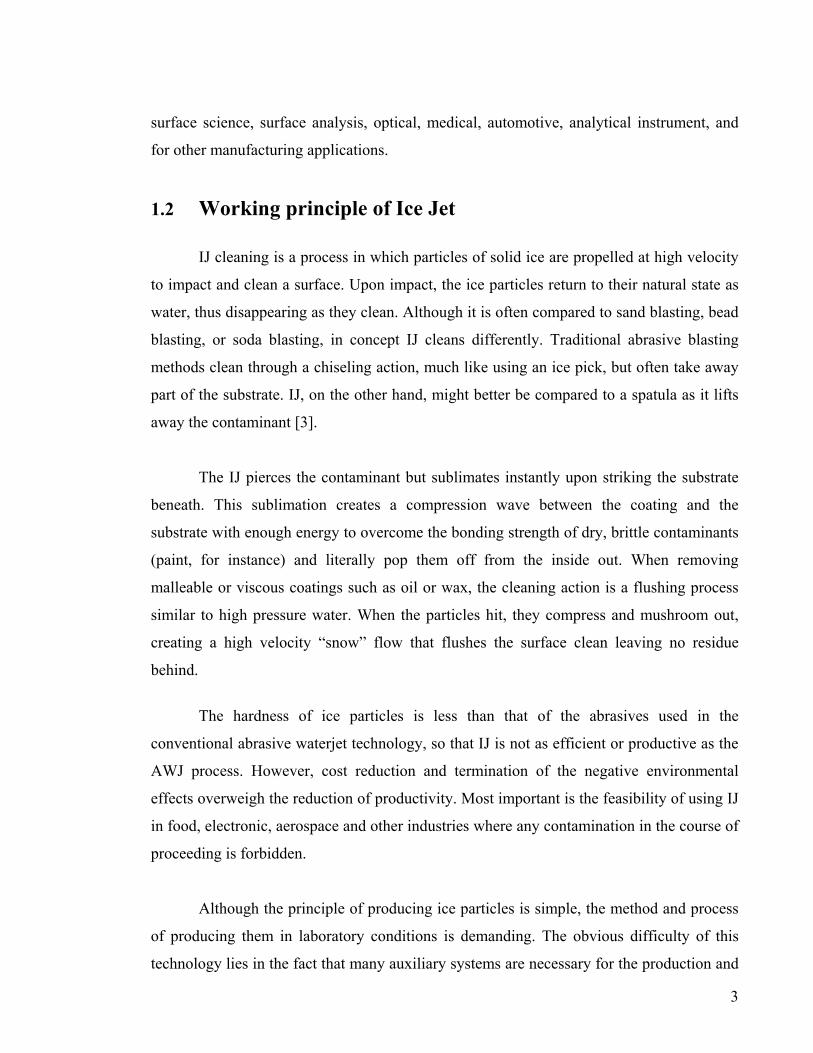
1.2 Working principle of Ice Jet

IJ cleaning is a process in which particles of solid ice are propelled at high velocity

to impact and clean a surface. Upon impact, the ice particles return to their natural state as

water, thus disappearing as they clean. Although it is often compared to sand blasting, bead

blasting, or soda blasting, in concept IJ cleans differently. Traditional abrasive blasting

methods clean through a chiseling action, much like using an ice pick, but often take away

part of the substrate. IJ, on the other hand, might better be compared to a spatula as it lifts

away the contaminant [3].

The IJ pierces the contaminant but sublimates instantly upon striking the substrate

beneath. This sublimation creates a compression wave between the coating and the

substrate with enough energy to overcome the bonding strength of dry, brittle contaminants

(paint, for instance) and literally pop them off from the inside out. When removing

malleable or viscous coatings such as oil or wax, the cleaning action is a flushing process

similar to high pressure water. When the particles hit, they compress and mushroom out,

creating a high velocity “snow” flow that flushes the surface clean leaving no residue

behind.

The hardness of ice particles is less than that of the abrasives used in the

conventional abrasive waterjet technology, so that IJ is not as efficient or productive as the

AWJ process. However, cost reduction and termination of the negative environmental

effects overweigh the reduction of productivity. Most important is the feasibility of using IJ

in food, electronic, aerospace and other industries where any contamination in the course of

proceeding is forbidden.

Although the principle of producing ice particles is simple, the method and process

of producing them in laboratory conditions is demanding. The obvious difficulty of this

technology lies in the fact that many auxiliary systems are necessary for the production and

3

transportation of ice particles. A significant amount of researches have been carried out for

the production of ice particles using stream freezing and supplying it in the water stream for

cleaning [4, 5]. It was reported that the addition of ice particles into the waterjet improved

the quality of cutting soft materials compared with a conventional plain water jet. The

feasibility of machining hard materials by ice particles generated in the course of water

freezing has also been demonstrated [6, 7]. Their work, however, showed the difficulties

involved with ice formation, sizing and concentration within a moving jet constricted in a

small orifice. Use of abrasive cryogenic jet to machine materials was also experimented,

wherein the abrasive particles were entrained by liquid nitrogen jet to form an abrasive

cryogenic jet [8, 9, 10]. It was shown that the abrasive-cryogenic jet had equal performance

to that of AWJ but without the liquid residue. The disadvantage of that is that, under current

cryogenic pumping technology, the cryopump, with high pressure and high flow rate whilst

maintaining cryogenic temperature, is not commercially available due to inherent

limitations. The other disadvantage is the cost of using pure liquid nitrogen.

There are some other techniques of producing ice particles. For example, it can be

done by mechanically crushing the ice cubes or by passing water mist through a cryogenic

fluid. The shortcomings of these systems include the necessity to have more additional

equipment to produce ice particles.

The proposed cryogenic jet system provides a novel method for cleaning and

surface processing that combines the thermodynamic effects of rapid cooling and the

mechanical action of the controlled impingement of ice particles. The system uses

cryogenic liquid nitrogen to cool water droplets exiting from a spraying system to produce

very fine particles. It is composed of an ultrasonic atomizer, a heat exchanger, ice particle

transfer tube and a delivery nozzle. This work studies the formation of the ice particles by a

novel technique and elucidates the fundamental mechanisms of the heat transfer through

computational fluid dynamics (CFD) modeling and experimental work.

4

1.3 Objective and Scope of the Project

The principal objective of this research project is to develop a competitive precision

Ice Jet system that utilizes cryogenic jets and then determine whether it is feasible to deploy

cleaning and blasting applications.

Specific objectives of the project include:

• Development of a new technique for ice particle formation and properties control

• Selection of water droplet injection system capable of producing droplets with

predetermined shape, size as well as controlled concentration and frequency

• Design and development of a heat exchanger capable of producing ice particles

• Design of ice particle transport system

• Investigate the mixing process with features of heat transfer, mass transfer and

momentum transfer between ice particles and water stream and to provide design

criteria for the Ice Jet nozzle

The above objectives are achieved through:

• Simulation of the heat transfer taking place inside the heat exchanger, inside the ice

particle transport system and inside the nozzle using Computational Fluid Dynamic

(CFD) software CFX

• Examination of the temperature distribution of ice particles on different planes of

the heat exchanger, and at various planes of the cleaning nozzle

• Visualization of the ice particle formation process using a high-speed camera

• Comparing modeling work with the experimental work and examining the

feasibility of using CFX in predicting the temperature distribution.

5

1.4 Organization of Research Work

Based on the objectives, the project was broken into several technical tasks, with a number

of sub-tasks:

1. Development of an effective atomizing system for producing water droplets

• Study of atomizing nozzle using ultrasonic

• Study of atomizing nozzle using pneumatics

• Study of conventional spraying nozzle

• Control of water droplets sizes

• Control of water droplets production rate (frequency)

• CFD modeling study of water droplet formation process and water droplets size

distribution

• Visualization study of water droplet formation process and water droplets size

distribution using Laser Doppler Anemometry (LDA), high-speed videography and

image analyzing techniques

2. Design of ice particle formation heat exchanger system

• Determination of heat exchanger unit materials

• Optimization of heat exchanger unit dimensions

• Effect of various additives mixed into water on the ice particle formation process

and its hardness

• CFD modeling study of ice particle formation process and distributions of particle

sizes and temperatures

• Control of ice particle hardness by controlling particle temperature and using

effective additives

• Visualization study of ice particle formation process using high-speed video camera

and image analysis technique

6

3. Design of ice particle delivery system

• Simulation of heat transfer inside the transportation system

• Length calculation of the transfer tube

• Variations of ice particle sizes and temperatures during delivery

• Necessity study of cold gas flow as ice particle carrier

4. Design of IJ nozzle

• CFD modeling study of mixing process between ice particle and water/air stream

inside the nozzle

• CFD modeling study of heat transfer and ice particle temperature and size variations

during mixing process inside the nozzle

• Study of ice particle temperature variation distributions at the exit of the nozzle

Parametric study of ice particle diameter, ice particle hardness, ice particle melting

rate and mass fraction are focused. This was done by experimentation and numerical

modeling, however, the numerical model was developed with the aid of experimental

results. The rate of change of ice particle was done by visualization experiments and

compared with few formulations of other research work in spray crystallization. The

numerical temperature study inside the heat exchanger was validated with experiments. The

numerical study of ice particle behavior in the transport system and jet nozzle was done to

find out whether the method used in this research is feasible and that, it can be used in

applications such as cleaning, blasting, drilling and at the most for cutting. The results

found through the various method of studying the process are integrated and generalized to

give an overall picture of the ice particle formation and melting process. These are finally

followed by general conclusions and recommendations for the future work.

1.5 Outline of Chapters

Chapter 2 details the literature review of the current state of knowledge in the Ice

Jet (IJ) with some emphasis on the Abrasive Water Jet (AWJ), Water Jet (WJ), Cryogenic

Jet (CJ) and Abrasive Cryogenic Jet (ACJ). Particular attention is given to the literature

7

concerned with ice particle temperature measurements by experiments and modeling which

are in track with the objectives and scope of this Ph.D. project.

Chapter 3 addresses the design criteria of the novel Ice Jet system. There are four aspects to

be considered:

• Selection of atomizer,

• Design of ice slurry heat exchanger system,

• Design of ice slurry transportation system and

• Design of ice jet cleaning nozzle

Chapter 4 explains the experimental set-up and procedure. Factorial designs, visualization

procedures of the Ice particle formation process are also given.

Chapter 5 develops the subject of Modeling and Computational heat transfer by relating the

available numerical procedures to the solution of differential equations governing heat

transfer processes.

Chapter 6 and Chapter 7 give details of the results obtained by experiments and comparison

with the results of numerical modeling. The temperature distribution, ice particle size

variation, mass fractions, effect of pressure and temperature on ice particle melting rate and

the effect of velocity of ice particles in the nozzle are investigated and discussed.

Chapter 8 contains a summary of the present research work together with general

conclusions and recommendations for the follow up work.

8

9

Chapter 2

Literature Review

2.1 Overview of the Review Process

The objective of the literature review is to acquire an understanding of the current

state of knowledge in the Ice Jet (IJ) process with some emphasis on the Abrasive Water Jet

(AWJ), Water Jet (WJ), Cryogenic Jet (CJ) and Abrasive Cryogenic Jet (ACJ) processes.

This was done by identifying and summarizing the research work that was reported by

various key researches in this field. To this end, the research work on various aspects of the

IJ that is reported in scientific journal publications, conference proceedings, trade journals

and other similar forums have been reviewed and summarized. Particular attention was

given to the literature concerned with ice particle temperature measurements by

experiments and modeling which are in line with the objectives and scope of this Ph.D.

project.

In the following sections, the historical development of WJ and AWJ cutting

processes is presented and is followed by CJ and ACJ processes. The development of IJ

process is documented in detail based on the available knowledge along with its

application. The ice particle formation process studied in other applications by experiments

and modeling were cited together with the physics of ice.

2.2 Various Jetting and Blasting Processes

2.2.1 Development of the WJ and AWJ Processes

The history of waterjet could be traced back to hydraulic mining of coal in the old

Soviet Union and New Zealand in early 1800s where it was used to wash over a blasted

10

rock face carrying away the loose coal and rock. However, some examples of much earlier

uses by Egyptians and Romans for other purposes have also been reported [11]. The water

used for mining operations was collected in a reservoir on a hilltop from streams and rivers,

which was then directed through pipes to the coal and mineral bearing rock surface. The

surface to be mined using this technique had to be weakened by using explosives owing to

the relatively low pressure of water jets [11, 12].

The introduction of high-pressure water jets for hydraulic mining was instrumental

in increasing productivity and reducing the cost of mining operations by making possible

the cutting of harder rocks without the use of explosives. Although it was possible to

generate very high pressure even higher pressure than that can be achieved with some

current systems, the method suffered from intermittent pressure, thus producing rough

operation that interfered with the production process. In spite of this, however, the high-

pressure jet remained the principal technique for hydraulic mining and other applications

until the 1970s at which time new pumping system was developed in USA that could

achieve a pressure of 4,000 bar thus tremendously advancing the technology [11, 12]

In the early 1980s, water jet cutting machines that integrated the new development

in pumping technology were installed, moving the water jet cutting technology closer to

wider acceptance as a relevant method for use in material cutting in industry. This was

accelerated by the entry in 1980 of Flow Industries and a number of other smaller players

into the market that contributed to the development of the technology [11, 13]. However,

the water jet machines that were available around this time were capable of cutting

effectively and efficiently only non-metallic materials such as wood, plastics, fiber glass

paper, cloth, and rocks of soft to medium hardness [11].

To increase the water jet cutting capability and improve cutting performance,

abrasive particles were introduced in the water jet stream in the early 80s. Although some

experimental work has been conducted and patents for a variety of such systems have been

granted in late 70s [14, 15, 16], practical abrasive water jet equipment was commercially

available for use in precision machining from the mid 1980s [17]. Substantial progress has

been made in the development, optimization and implementation of the technology for

various industrial processes in the last fifteen years. However, some outstanding technical

issues associated with the use of the technology are still to be addressed [18]. Figure 2.1

shows the modern abrasive water jet cutting machine manufactured by OMAX.

Figure 2.1 OMAX 2652p Pictured with Automatic Z-axis

The energy transfer and subsequently the mode of material removal changed

dramatically by addition of abrasive particles into the water stream. The Abrasive Water Jet

(AWJ) generated as the result of such an addition enables machining practically any

engineering material. The rate of removal of “hard-to-machine” by the use of AWJ is

comparative if not superior to other material removal processes. Due to its capability, AWJ

in a short time became one of the leading machining technologies. In the course of AWJ,

particles are sucked into the mixing chamber due to the vacuum created by the jet. Mixing

of water and particles and formation of homogenous flow occurs in a focusing tube, which

forms a highly erosive slurry jet. The various applications of AWJ are well understood and

documented [19].

However, AWJ is a mixture of water and particles and this imposes a number of

limitations and inconveniences. The energy efficiency of AWJ is still low, but acceptable.

11

12

Mixing of water and particles imposes a severe limitation on the minimal usable jet

diameter and special provisions are required for particles supply and disposal. Furthermore,

the addition of abrasive particles increases the cost of processing and its environmental

impact.

2.2.2 Cryogenic Jets

In some applications the use of Water Jet or Abrasive Water Jet is not compatible.

Such applications include processing hygroscopic and chemically reactive materials and, in

some cases, jobs performed in close proximity to high-voltage, toxic, and radioactive

sources [20]. For processing toxic and radioactive materials, used water and abrasives

become contaminated, therefore it is difficult and expensive either to be treated or for

disposal. For these methods cryogenic jets were developed that involves usage of high-

pressure liquid nitrogen jet, high-pressure carbon dioxide jet and abrasive cryogenic jet. All

these processes employ cryogenic jet as the high-pressure fluid [20]. Research has been

undertaken in using cryogenic jets and abrasive cryogenic jets for various applications [21].

The ability of the cryogenic jets at cryogenic temperatures to be chemically inert or

inactive, non-explosive and biologically sterile has made them suitable for a number of

applications. For example, liquid nitrogen jets find applications in the food industry and for

cleaning, stripping, paint removal, and nuclear decontamination and decommissioning.

Ammonia jets are used in demilitarization of chemical weapons. For these classes of jets,

thermodynamic control of the upstream (and sometimes downstream) conditions is critical

[22].

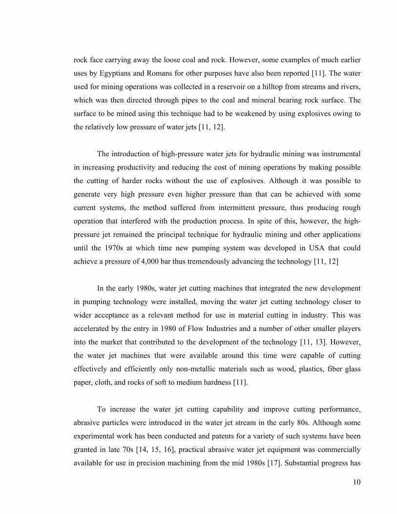
2.2.2.1 CO2 Jet

Among the thermodynamically unstable fluids, the most practical application is

found for carbon dioxide. Conventionally, CO2 is contained in bottles at temperature of

25°C. The equilibrium at this pressure is 67 bars as shown in Figure 2.2. At these

conditions, carbon dioxide exists as saturated liquid [23]. At the nozzle exit, the fluid

pressure drops to 0.1 MPa. At this pressure, the temperature of the carbon dioxide drops to

–78°C and the liquid is converted into a mixture of gas and solid.

Figure 2.2 State diagram of Carbon dioxide [23]

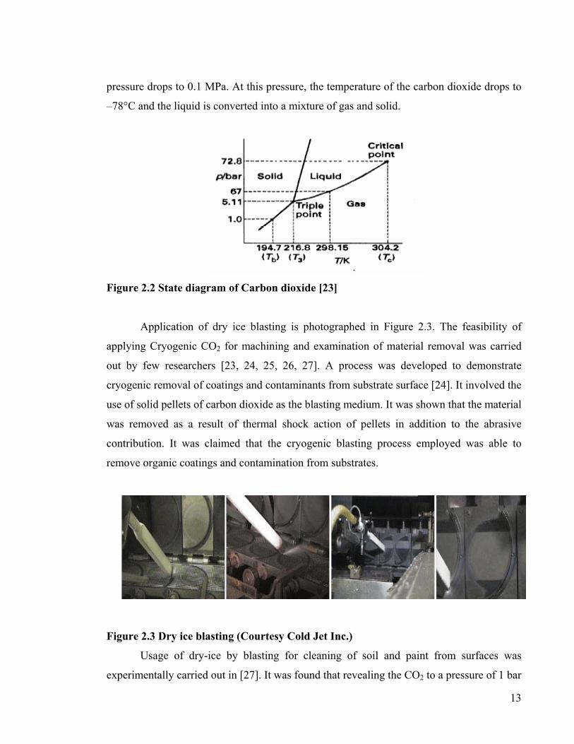
Application of dry ice blasting is photographed in Figure 2.3. The feasibility of

applying Cryogenic CO2 for machining and examination of material removal was carried

out by few researchers [23, 24, 25, 26, 27]. A process was developed to demonstrate

cryogenic removal of coatings and contaminants from substrate surface [24]. It involved the

use of solid pellets of carbon dioxide as the blasting medium. It was shown that the material

was removed as a result of thermal shock action of pellets in addition to the abrasive

contribution. It was claimed that the cryogenic blasting process employed was able to

remove organic coatings and contamination from substrates.

Fi

ex

gure 2.3 Dry ice blasting (Courtesy Cold Jet Inc.)

Usage of dry-ice by blasting for cleaning of soil and paint from surfaces was

perimentally carried out in [27]. It was found that revealing the CO2 to a pressure of 1 bar

13

14

at a temperature of -80°C generates dry-ice snow. The hardness of the pellets formed was

claimed to be between 2 and 3 Moh’s, similar to the hardness of gypsum. Diameter,

distribution, velocity of dry-ice particles and their impact force were studied. It was also

revealed that the process could be applied for removing silicone seals without any

significant surface damage.

Preliminary parametric study of drilling and cutting performance was carried out by

using liquefied CO2 jet at pressures ranging between 35 and 350 MPa [23, 25, 26]. The

observations revealed no evidence of brittle fracture in aluminum. The cutting power of the

jets was claimed to decrease with the stand-off distance, but on the positive note could be a

desirable characteristic for applications in which damage to materials must be avoided.

However, the recommendations suggested using liquid nitrogen instead of liquid CO2 due

to the unstable nature of liquid CO2. The thermodynamically unstable liquid CO2 changes

phase to gas as it moves downstream, causing the jet to expand and decelerate [28]. A

condition was reached at which the energy flux impinging upon the workpiece was

insufficient to remove material. It was suggested that this could be applied where substrate

damage was not intended.

Thus due to the inherent thermodynamically unstable nature of the liquid CO2,

industrial attention was focused on using liquid nitrogen jets for the development of useful

cutting and surface-preparation tools.

2.2.2.2 Liquid Nitrogen Jet

The thermodynamics of jet formation of liquid nitrogen jet was demonstrated when

the fluid was adiabatically throttled through an orifice [22]. The variation of jet coherence

with temperature and pressure was studied and its cutting power was shown to be poor.

However, from the visualization experiments it was stated that as the temperature

decreases, the visible portion of the coherence improved. Figure 2.4 shows the Ultra High

Pressure liquid nitrogen jet.

The use of cryogenic liquid nitrogen for cutting is not reported, however, its use for

cooling and freezing purposes has been reported in [29]. It was used for drilling ground in

unconsolidated formations.

Motor Pump

Burst Disk

Nozzle Sub-cooler

Burst Disk

UHP Cryo valve

Pressure Gauge

Surge Chamber

Jet

Work Piece

Relief Valve

Bulk Storage

LN2 transfer line

Sub-cooler LN2 supply line

Figure 2.4 Schematic of Ultra High Pressure Liquid Nitrogen Jet [30]

Liquid nitrogen was used in milling experiments to increase the tool life by using it

as a cryogenic cooling media [31]. It was also shown that the use of liquid nitrogen for

cooling in grinding increases tool life [32]. A different type of research was done to

atomize liquid metals by the use of liquid nitrogen [33]. The results indicated that as the

pressure increased the size of super fine particles decreased and was observed to be

spherical.

15

16

2.2.2.3 Liquid Ammonia Jet

Ammonia has been used for years as a cryogen in different applications. Recently,

however, liquid ammonia was demonstrated to be useful in efficiently and rapidly

demilitarizing rocket motors [27]. Energetic ingredients such as AP, HMX and RDX are

soluble in ammonia and thus, can be washed out. Gel and solid rocket propellant can be

physically and chemically ablated from motors using a liquid or gaseous reagent such as

anhydrous ammonia [34]. It was projected that the high pressure ammonia jets can be used

to cut steel and aluminum rocket casings [22]. At ambient temperature, ammonia is

liquefied at 0.78 MPa and thus to form an ammonia liquid jet at room temperature. Even

with the use of liquid ammonia, however, to cut metals, abrasives need to be added to the

ammonia jet [22].

Low penetration rate, high volumetric flow, less impact on surface were some of the

disadvantages of the Cryogenic Jets. In order to increase the impact strength, abrasives

were added along with CJ to form Abrasive Cryogenic Jets (ACJ).

2.2.2.4 Cryogenic Abrasive Jet

The principle used was similar to AWJ but instead of using high-pressure

abrasive/water mixture, liquid nitrogen, liquid CO2 or liquid Ammonia was used [3]. In

conventional AWJ nozzles, abrasive particles are entrained into the jet by the Bernoulli or

“jet pump” effect. The high-speed jet creates a low-pressure region inside the nozzle which

draws particles through an abrasive port and feeds them into the nozzle. In Abrasive

Cryogenic Jet (ACJ) when used with liquid nitrogen, the abrasives was fed by dry nitrogen

carrier gas instead of ambient air flow, since the ambient air becomes moist due to the

liquid nitrogen flow. In this research it was also found that the abrasive feed method used in

conventional AWJ nozzles was ineffective to be used for cryogenic jets because of high

back pressure. In case of liquid ammonia jets, the entire abrasive hopper was laced inside

the ammonia chamber. CO2 abrasive was generated directly in the ACJ nozzle through

rapid Joule-Thomson cooling of the liquid. The technique was used for in situ creation of

CO2 dry ice for surface treatment (cleaning and stripping) [8, 9, 10].

17

Another research was done on the parametric study to explore the potential use of

ACJ's for cutting of metals and brittle materials [35]. Low pressure liquid nitrogen jets were

used along with garnet abrasives to find out the performance. The results of the research

showed that the AWJ performed better than the ACJ due to the better alignment of waterjet

in the abrasive mixing tube rather than the intrinsic differences between the two processes,

but there was no liquid residue found.

It was also shown that Vanishing Abrasive Cryogenic Jet (VACJET) can be used

for removing coatings on delicate substrates for recoating [21, 36]. CO2 particles were

added to the cryogenic liquid nitrogen jet to increase the stripping power. However it was

claimed that due to the less aggressive nature of the VACJET compared to the ACJ the

damage to the substrate was minimized.

A similar research was done in applying CJ and ACJ in applications such as aircraft

de-painting, access hole cutting and nuclear facility decontamination & decommissioning

(D&D) [20]. The use of CJ/ACJ was compared to WJ/AWJ in the study and revealed that it

showed promise on the application side, but was same or in fact less on the performance

side due to the lack of energy. In de-painting applications it was shown that no irregular

breakup of the paint edges resulted. In access-hole and nuclear D&D the CJ/ACJ vanishes

upon impact.

2.3 Development of Ice Jet Technology

To this context of the literature survey various cryogenic systems for different

applications are reported. From these reports it is found that the application ranges of the

processes are highly limited and can only be used where it is very essential. The processes

are highly expensive and their application for sensitive surfaces is not probable. This is due

to the fact that the substrate would damage or would crack under very low temperature. The

fact that, cryogenic jetting can only be operated at low pressure limits its ability for cutting.

The operating pressure and temperature range of the cryogenic pump is limited and its

operating and maintenance costs are very high. The transportation of cryogenic fluids under

18

pressure is subjected to risk and requires high safety standards. These factors helped the

development of another technology called Ice Jet.

Ice jet can be compared to the widely known chemical cleaning. Chemical cleaning

is an effective and competitive surface processing technology. However, the environmental

legislation and public awareness limit the use of this technology. A number of alternative

processes have been explored in order to replace chemical cleaning by an environmentally

acceptable surface processing technology [19]. The practice demonstrated that the most

realistic replacement of the chemical treatment is water blasting. It was found that in most

cases jet cleaning not only meets technical specification, but also in a number of cases is

the most effective technology. However, significant deficiencies impede adoption of the

water blasting. The water consumption for decoating is comparatively high. The disposal of

this water is environmentally damaging, while water recycling is comparatively expensive.

Water impact might cause substrate damage, while insufficient water velocity results in low

productivity. Also specialized facilities are needed for water jet cleaning.

The addition of abrasives into the Water Jet, that is formation of the Abrasive Water

Jet, dramatically improves process productivity. This, however, results in the potential

contamination of the substrate as well as in the generation of the difficult to deal with

emission. The pollution will be eliminated if a benign abrasive material, for example water

ice, is used to enhance material removal. The replacement of the abrasive water jet by the

mixture of water and water ice will combine competitive process productivity with its green

nature.

It is highly desirable to enhance the productivity of WJ and avoid solid emission.

This objective could be achieved by the replacement of conventional abrasive materials by

ice particles, thus resulted in the development of new technology called Ice-Water Jet (IWJ)

[19]. The use of ice, as solid particles, would erode the material in the impingement site due

to their inherent properties. Termination of the negative environmental effects of AWJ

machining constitutes a significant advantage of IWJ. Most importantly, however, is the

feasibility of using IWJ for shaping of food, electronic components, space and other

branches of industry where any contamination in the course of processing is not permitted.

19

Another potential application of IWJ is in medicine. The detailed literature of the

applications is given in Section 2.3.2. If ice particles are produced by cryogenic fluids

rather than using cryogenic fluids as the main stream, then the cost of producing such ice

particles is less. It is, however, not necessary to store the ice particles as they have to be

produced “Just-In-Time”. So this constitutes the ice particles for “in situ” applications.

It is highly desirable to convert an environmentally unfriendly, but widely adopted,

AWJ machining into a “green” ice blasting process. However, it is necessary to overcome

significant technological difficulties in order to attain adoption of IWJ by industry. The

erosion of substrate by impinging particles is due to stress waves generated in the course of

impact. The strength and duration of these waves depends on mechanical properties of the

impinging particles. The elastic characteristics of conventional abrasives are superior to that

of ice. Thus, these abrasives constitute much more effective machining tool. Despite its low

productivity, the use of such Ice Jet would be highly suitable in food, biomedical and other

industries where the contamination of the substrate constitutes the primary concern of

users.

The use of particles as energy carriers in the impingement zone is one way of

improving momentum transfer between the fluid and the substrate. The increase of the

density of the fluid momentum at the impingement zone is another approach to this

problem. Highly coherent fluid flow readily passes through a layer of a rejected fluid. Thus,

momentum losses of the jet are reduced. However, the mechanisms of the energy delivery

to a substrate by a coherent jet and impacting particles are quite different. Material removal

by particles is due to erosion, while penetration of a fluid jet is due to stagnation pressure.

Due to this, even coherent jet can penetrate only comparatively soft materials. The most

effective way to increase jet coherence without water contamination is by addition of small

amount of polymers [11, 37]. The improvement of the jet penetration by addition of

polymers is widely adopted by industry.

The most important problem, which needs to be solved, is the difficulties in the

generation and handling of ice abrasives. Regular abrasives are stable at all practical ranges

20

of operational conditions, while ice particles can exist only at subzero temperatures.

Maintaining such a temperature within the nozzle and within the jet is an extremely

difficult task. Ice particles have a tendency to coagulate and thus can block the transfer

lines, ice jet nozzle and focus tube. The adherence between the particles increases

dramatically, as the temperature approaches 0°C. Thus, ice particles have to be fed either as

particles or to be entrained by cold gas, transportation medium in order to maintain

segregation. In order to assure the acceptance of IWJ by industry, it is necessary to develop

a practical technology for formation of ice-water slurry [38].

2.3.1 Air Ice Jet

The use of ice particles is simplified if the particles are entrained in the air stream

[19]. Current cleaning technologies are based on the use of chemicals or sand and water

blasting. All of these technologies bring about heavy environmental pollution. The Air-Ice

blasting constitutes a unique cleaning technology, which involves practically no off-

products and thus has no negative environmental impact [19]. Ice blasting could be used in

the elimination of the consequences of chemical and biological attacks. Currently, ice is

used as cooling media for food preservation. It is used as fine ice powder and this reduces

food cost and improves quality.

There are several other reports of the application of the Air-Ice Jets [2, 39, 40]. The

advantage of an air driven system is the feasibility of maintaining a low temperature of the

stream and a high-pressure gradient in suction lines. Because of this ability it is possible to

use them for cleaning engineering purposes. However, the machining ability of the Ice Air

Jet is insufficient for removal of the most engineering materials. Thus, IAJ can be applied

for surface processing, while the material shaping will be carried out by IWJ.

A number of surface processing technologies based on the use of the air-ice stream

have been previously suggested [19, 41]. The first of such technologies was a car washing

machine, utilizing ice particles. The stream of frozen particles controlled by a set of coils

was directed at surfaces to be treated [42]. The cleaning of the sensitive surfaces by the

21

impact of fine grade ice entrained into the air stream was proposed by Szijcs [43]. The

atomization of liquid in air stream and subsequent freezing of the generated fine droplets

formed the blast material. The freezing was achieved by the addition of refrigerant (N2,

CO2 and Freon) into the stream in the mixing chamber or by the addition of refrigerant into

the jet after the mixing chamber. Another technology involved the use of ultra clean ice

particles, having the uniform grain size, for cleaning surface and grooves of ferrite block

[44].

Ice blasting device utilizing stored particles was suggested by Harima [45]. The use

ice particles near melting temperature for surface cleaning by ice blasting were investigated

by Vissisouk and Vixaysouk [46]. An ice blasting cleaning system containing an ice

crusher, a separator and a blasting gun was developed by Niechcial [41]. Production of ice

particles less than 100 micrometers in size inside the apparatus and just prior to the nozzle

was suggested by Settles [5].

The substantial advantage of IAJ is elimination of off-products, solid or liquid, while its

disadvantage is the use of gas as a source of momentum. Low density of the gas media

limits machining ability of the jet. The use of cryogenic fluid (liquid nitrogen, ammonia and

carbon-di-oxide) enables to eliminate off-products as well as substrate contamination, while

the sufficient momentum is delivered to the impact zone [23]. The obvious difficulty of this

technology is the necessity to maintain a working fluid at a cryogenic temperature. The

detailed literature of the cleaning is given in Section 2.4.

2.3.2 Water Ice Jet

There are several possible techniques for formation of Water Ice Jet (WIJ). Ice

particles can be produced separately and then injected into the water stream similar to

abrasive particles [38]. In this case, at least in principle, the generation of the ice particles

of the desired dimensions, having maximal hardness could be feasible. The obvious

shortcoming of this technology was the need of auxiliary systems for the particles

production and transportation.

22

Water Ice Jet could be created by the formation of ice particles in the course of jet

expansion in the nozzle. Thermodynamics of ice [47] shows that it is possible to reduce the

temperature of compressed water much below 0°C without freezing. At the pressure of 13.8

MPa, water temperature could be reduced down to -25°C. During the expansion in the

nozzle, while water pressure reaches 1 bar part of water would convert to ice. Due to

enthalpy release during the solidification, water temperature increases, but it should be

contained below 0°C. The fraction of water converted into ice can be determined by the

difference between water enthalpies prior and after the nozzle and also by enthalpy

conversion into kinetic energy of the stream during water acceleration. The shortcomings of

that technology were the difficulties of the control of particle nucleation and, most of all, a

small margin of enthalpy available for solidification.

Finally, ice formation is possible by cooling compressed water prior to the nozzle and

additional water cooling in the focusing tube. Heat removal in the focusing tube was

attained by submerging the focusing tube into a cooling media [48]. These techniques

enabled to increase the rate of ice generation, but resulted in increase of WIJ diameter due

to the use of the focusing tube. However, in that case, the focusing tube was not used for

mixing of water and particles. Due to that, the diameter of the focusing tube and thus,

stream diameter was significantly less than that during particles addition. Cooling of the

focusing tube required much simpler facility than preparation and handling of ice particles.

Thus, each of these techniques has its own disadvantages and shortcomings as well

as benefits. Further research is required to improve these technologies.

2.4 Applications of Ice Jet

2.4.1 Ice Jet cleaning

The cleaning and abrading surfaces with ice-blasting technique was demonstrated

by Galecki and Vickers [49]. Ice particles of approximately 3mm diameter were produced

by crushing mechanically ice cube of diameter 30mm. The ice cubes were placed in a

23

container having liquid nitrogen where they were further cooled and then transferred to a

mechanical crusher where they were crushed and subsequently entrained into a nozzle

through which the high velocity compressed gas was flowing. The results suggest that the

ice abrasives jet shows a sufficient machining effect in cases where, ice particles of very

low temperature were used. It was concluded that the ice-blasting technique was shown to

be more effective than both water jets and percussive needles, but not as effective as grit-

blasting. For cleaning applications where the grit blasting could not be tailored, the ice

blasting would be a very promising technique.

Application of ice particles for precision cleaning of sensitive surfaces such as

compact discs and electronic boards was carried out by Geskin [2]. Ice particles were

formed by mechanical crushing. FIDAP software package was used to determine the

probability of particles surviving in the course of the jet formation. The operated nozzle

diameter was 5mm and the ice particles were of 2 to 5mm in diameter. Use in cleaning of

electronic boards, decoating of sensitive surfaces, decoating of soft substrates, restoration

of electromechanical devices, removal of highly adhesive surface layer and etching

applications were demonstrated.

Investigation of the entrainment of ice particles by water jet was done by both

experiments and simulations [7]. It was demonstrated that at the optimal range of process

conditions this jet constituted a precision tool for selective material removal operations.

Experiments carried out focused on degreasing, depainting and de-icing of liquid crystals,

polished metals, optical glass, fabric, removal emulsion from a film, etc. The feasibility of

the damage free and pollution free decontamination of highly sensitive, highly countered

surfaces was demonstrated.

Few patents were also found in using ice jet for cleaning. An apparatus for

producing ice particles was developed by Settles [5]. The apparatus consisted of a pressure

reservoir, a mixing chamber, a flow spreader, a pneumatic atomizer and a freezing

chamber. Fine ice particles were produced and were basically designed for cleaning

applications. Another apparatus for polishing surfaces by generating low hardness ice

24

particles was developed by Hisasue [4]. The process involved producing super fine ice

particles by mixing liquid nitrogen and atomized water droplets. A gettering method for

semiconductor wafers, which comprised of blasting frozen particles at the surface of

semiconductor wafers, was developed by Tada [50, 51]. The ice particles were formed by

spraying fine mist of water into a chamber partially filled with liquid nitrogen.

An apparatus for blasting crystalline ice was devised by Visaisouk [46]. Ice

particles were impacted on a surface and it was found that erosion was effected by the

rupture process caused by the well-known reaction force. Decontaminating of sensitive

surfaces was investigated by Geskin [6]. Electronic boards of various electronic devices

were contaminated with grease and metal powder and were cleaned with ice blasting. It was

claimed that the boards worked normally. Suggestions from the research indicate that, at

sufficient kinetic energy ice particles could be used for machining of metals, ceramics and

composites. There are several patents available on using Ice Jet for blasting [52, 53, 54]. A

method of producing ice particles by cooling the water jet in the discontinuous region using

liquid nitrogen was proposed [55, 56, 57, 58], which was later used for cleaning

applications.

2.4.2 Ice Jet for Machining

An experimental approach using ice jet for drilling steel, aluminum, titanium and

composite samples was developed [19]. The results of machining were compared with that

of waterjet and was demonstrated that it is feasible to use of ice-water mixture as a

machining tool by replacing abrasive waterjet in certain applications. The experiments

indicated the effectiveness of material removal by Ice Jet, which was strongly correlated

with the size and temperature of ice particles. However, problem of clogging was a main

concern and was found that if the part of the supply line was maintained below 0°C, it

could be prevented. The schema of the Ice Jet system is shown in Figure 2.5.

Figure 2.5 Schematic of Ice Jet System for Drilling [19]

A method of cooling high-pressure water jet by cryogenic compressed air was

developed [59]. The method was used in drilling using ice abrasive jet. The effect of water

droplet diameter, droplet temperature in still cryogenic fluids was presented.

A work was performed to use Ice Jet as a machining tool [7]. Ice particles were

supplied into water stream directly and also by generation within the stream by cooling

water prior to and after expansion. An improvement of Ice Jet technology was carried out

with the possibility of using it for cutting [48]. It was postulated that cooling of water prior

to the nozzle does not constitute the necessary condition of Ice Jet formation but, cooling of

the water stream after the exit of the nozzle could generate ice particles. Precision control

of the heat removal from the water stream was required for particles formation. The

addition of ice to WJ completely changed the mode of the jet-substrate interaction. It was

concluded that the width of the kerf was equal to WJ and was less compared to AWJ.

25

26

2.4.3 Biomaterial

A study was undertaken to investigate processing biomaterials [60]. It was tried to

enhance the cutting efficiency by mixing pellets of crystalline ice into the stream of pure

water jets. Several different approaches for entraining the ice pellets into the jet stream

were tested in the study. It was concluded that, theoretically, it could be possible to obtain

the ice particles in the water jet. In practice, the presence of separated ice particles in the

water jet was limited to narrow range of experimental conditions. Controlled removal of

epidermis layer of skin from the skin surface was also demonstrated [38]. It was also shown

that the skin layer could also be removed with deeper penetration.

2.4.4 Nuclear

In the nuclear industry, operations such as cutting or rubblising of hazardous

materials and processing toxic/reactive chemical wastes, solid rocket propellants, and a

wide range of aging munitions are routinely performed. Potential use of ice jet technology

for removing explosives from the shell was investigated [61]. A relatively new method for

dismantling obsolete ammunition satisfying the requirements of increased productivity with

guaranteed process safety was proposed by using ice particles. A complex mathematical

model with the combination of hydrodynamic and thermodynamic processes, which

describes the use of water ice particles, was developed.

2.4.5 Potential Application in Surgery

Joint replacement has become one of the most common operations in orthopedic

surgery. For fixation of the prosthesis to the bone, both cemented and un-cemented

fixations are used. Cemented or un-cemented components for total hip or knee arthroplasty

have to be removed. Some techniques like ultrasonic tools and lasers have been developed

and tested, but the heat induced during cutting limits, their application. Experiments were

conducted to study the possibility of using plain water jet cutting [62]. Cadaver bovine

femora and femur bones were taken and cut. It was concluded that Poly Methyl

27

Methacrylate (PMMA) was cut better than bovine bones when plain water was used. It was

proposed that the use of Ice Jet could enhance the cutting of bovine bones.

2.4.6 Numerical Modeling of Ice Jet

Very little research has been carried out on the modeling and simulation of Ice Jet.

Development of a model for the growth of ice particle formation was carried out by Hiroshi

[63]. A simple model to understand the phenomena of ice nucleation was developed.

Calculation of the model was based on the following hypothesis:

• Circumferential cryogenic fluid is gas; having temperature, T, near each boiling point

temperature of liquefied CH4/H2 at atmospheric pressure.

• A water droplet solidifies in a certain time. Therefore, natural convection might appear

in the droplet during the solidifying process. However, the water droplet was considered

as a quasi-solid, since the droplet was cooled rapidly and that resulted in ignoring

convection inside the droplet.

• The droplet was assumed to be spherical as the droplets are very small in diameter.

• The water droplet at the lowest limit of relative velocity U (U=0m/s) is cooled down by

the natural convection.

• It is not clarified until what temperature the super-cooling phenomena occurs when the

water droplet of small diameter is cooled with very high cooling rates.

It was concluded that as the size of the droplet increases the time taken for freezing

increases. Also as the relative velocity of the droplets increases the freezing time decreases

and as the droplet diameter increases the critical flight distance to freeze increases.

The study of survival of ice particles inside the focus tube of the water jet nozzle

was carried out by Ahmed [64]. The impact of different inlet ice particle temperatures

(-50°C, -40°C, -30°C, -20°C and -10°C) over the ice particle exit temperatures were

calculated. It was concluded that water and air temperature play an important role for the

28

existence of ice particles at the exit of the focus tube. It was shown from simulation results

that ice particles survived at the exit of the focus tube at 0°C inlet temperatures of the jet or

below.

Ice particle trajectory and particle distribution inside the mixing chamber was

modeled using FIDAP [19]. It was predicted that excess residence time in the mixing

chamber causes ice particles to melt in a shorter time. High velocity water jet also has a

high impact on melting of ice particles and finally, high turbulence at the entrance of the

focusing tube also melts ice particles at a higher rate.

The use of ice blasting technology for removing explosives was performed using a

complex mathematical model [61]. The disintegration of the turbulent jet and its loss in

energy was simulated on the basis of similarity theory using empirical information.

Dispersed flow with multi phase equations were solved by a set of differential equations.

The interaction between the solid ice particles and the explosives was considered with

particle equations. It was claimed that the developed software was capable of providing

calculations for the improvement in mass productivity of dismantling.

To this extent, literature about WJ, AWJ, CJ and ACJ with greater emphasis on Ice

Jet are given. The processes of WJ and AWJ are well documented, as the process is

commercially viable and improvements in optimization and its applicability are highly

desirable. In fact WJ and AWJ are well established in industry and owing to their high

productivity and reliability their negative effects such as, high recycling cost and high

volume of secondary debris do not constitute a serious short fall of the processes.

CJ and ACJ are techniques used among researchers and their feasibility as practical

technologies is not well recognized as the applications are limited. The serious drawback of

the processes is their high operating cost although this is not applicable in applications

where WJ or AWJ are not feasible.

29

The application of IJ has been investigated by many researchers experimentally.

The use of numerical simulations on the turbulent Ice Jet was also predicted by few

researchers. Research was concentrated on the effect of Ice Jet outlet parameters of the

nozzle and focus tube for machining of soft and brittle materials. Although it is desirable to

establish a parametric insight of the mixing nozzle, knowledge of the formulation of ice

formation process parameters is also highly desirable in arriving at a deeper understanding

of the entire process in the system.

However, the focus of the research work to date has been mostly qualitative and

only paid a cursory attention to the ice particle temperature and their efficiency of

production. In general, as the review of the literature in Section 2.4 has shown, the ice

particle formation process involving temperature measurements, ice particle size and the

atomization methods are not clearly explained.

The temperature transitions of freezing droplets are of major importance for various

applications. Although work on the temperature distribution and/or the freezing times of ice

particles is very scarce in the literature, theoretical and experimental work has been

reported on spray crystallization of ice particles for refrigeration applications. However,

these applications are quite different from the study reported here. This work is reported in

the following sections, and in general the various experimental and numerical

methodologies adopted in these studies were applied in the present study with few

modifications.

Although the principle of producing ice particles is relatively simple, the method

and process of producing them in laboratory conditions are demanding. The apparent

difficulty of this technology lies in the fact that many auxiliary systems for production and

transportation of ice particles are necessary. The literature following outlines some of the

research done on temperature transitions on spray crystallization. Numerical phase change

along with heat and mass transfers occurring in various problems are also sketched as it

was considered relevant and beneficial to the present research study.

30

Transient heat convection associated with phase change is an important

phenomenon to this study as it assists in the analysis in the temperature distribution.

Although the equations governing such problems are often easily derived, the solution of

these equations has proven to be difficult even for simple problems. These difficulties arise

primarily because of the unknown location of the solid-liquid interface that renders the

governing equations nonlinear [65]. Phase change problems can be solved for many

geometry and boundary conditions like the energy dissipated onto the work piece and heat

generated/dissipated from surroundings. It is emphasized however, that both the phase

change problem and the single phase problem have the same governing equation called the

diffusion equation. Thus a phase change problem can be solved by solving an equivalent

single phase problem with approximately specified boundary conditions. The phase change

problem takes advantage of the fact that a pure substance will absorb or release heat during

phase change at a fixed temperature. The exchange of latent heat is feasible at lower

temperatures and depending on the substance the magnitude can be far greater than the

corresponding sensible heat exchange for the same temperature difference [65].

The studies that are relevant to the current study were classified into Spray

Crystallization, Visualization experiments, Numerical simulations, Refrigeration and

Modeling.

2.5 Spray crystallization

Studies to examine the water spray method of ice slurry production for spray

cooling were carried out in [66] and [67]. In these works, spherical ice particles of less than

300µm diameter were produced by spraying water into a vacuum chamber where the

pressure was maintained below vapor pressure of ice and the temperature below the

freezing point of water. A theoretical investigation using diffusion controlled evaporation

model was also proposed. In the model, the rate of change of mass reduction of a droplet,

rate of variation of droplet size and surface variation of droplet temperature was

formulated. The results of the experiments were compared with the theoretical formulations

and have claimed to agree well. Latent heat of heat transfer was used for phase change.

DShanmugam

Introduction to the problem

31

With enough residence time, chamber pressure below triple point and small droplet size, ice

particles could be formed with the initial droplet temperature of 20°C. An optimizing chart

for transportable ice slurry using the relation of the residence time of a droplet in the

chamber, the injection pressure, the spray droplet size and the chamber pressure was also

proposed.

An experimental and numerical technique to study the temperature transition of

freezing droplets in spray crystallization was reported by Hindmarsh [68]. In the

experiments an intrusive method of levitated droplet suspended on a thermocouple was

studied with a cryogenic gas passed over it. The process was recorded using a video camera

and that facilitated the observation and analysis of all different stages of cooling and

freezing. Following that, several models with different phenomenon were developed in

order to systematically describe the observed process. The model incorporated assumptions

of conditions with constant property and with changing property. It was predicted that the

convergence of the solid cooling stage increased with the addition of changing thermal

properties and Ranz and Marshall Model [69] has good applicability to dual heat and mass

transfer.

An experimental and theoretical study on heat and mass transfer on freely falling

droplets in various environments was reported by Yao & Schrock [70]. In that work it was

postulated that for cooling of airborne droplets in a cold atmosphere, heat transfer occurs by

three main mechanisms: convective heat transfer, convective mass transfer and thermal

radiation from the droplet surface. It was also demonstrated that there are two ways to

model the internal heat transfer of a droplet: one by solving the internal temperature profile

by describing internal conduction and the other by assuming a uniform temperature within

the droplet. The assumption of a uniform temperature meant that the transient heat transfer

of the droplet could be predicted by balancing the heat flux from the surface by heat and

mass transfer with the internal energy of the droplet. It was concluded that the uniform

temperature within a droplet was a product of internal mixing of liquid within the droplet.

Drag of a mono-disperse droplet moving in an infinite droplet chain investigations

with numerical and experimental methods was reported by Liu [71]. It was predicted that as

32

the droplet spacing increases the drag coefficient increases. This solution was obtained by

dividing the flow field into two regions, the inner domain, where the flow was influenced

strongly by the spherical particles, and the outer domain, where the flow was essentially

parallel to the axis. The prediction of the drag coefficient of droplets in an infinite droplet

chain was found to be an order of magnitude smaller than the drag coefficients of a single

droplet in an unconfined parallel flow.

The research on spray crystallization gives a glimpse of approaches that can be

adopted for the research in ice particle formation. However, the approach in the current

study is different with the ice particles formed inside a heat exchanger.

2.6 Numerical Simulations of Phase Change Problems

A numerical prediction method for a turbulent two-phase flow in a vertical channel

with a Lagrangian approach was obtained by Sommerfeld [72]. It was shown that the

particle velocity fluctuations increased considerably when irregular bouncing particles were

incorporated in the calculations. However, the prediction showed that, when comparing the

simulations with those using the ideal wall collision models the modifications of the

particle phase properties for the small particles were found to be less pronounced than those

for the large particles.

The effect of free and combined convection on the mass transfer was found in the

report of Adekojo [73]. Numerical simulations of the mass transfer of droplet in a

continuous phase were done for conjugate problems. The mass transfer process was solved

by Navier-Stokes and the convection-diffusion equations using finite element method. It

was reported that the Navier-Stokes equations were modified through the Boussineq-

approximation to account for the effect in density with concentration. The effect of

combined free and forced mass transfer was numerically simulated.

A three-dimensional numerical procedure has been used to predict the behavior of

spherical and deformed droplets in gas flow [74]. In that research it was said that a

computational grid moving with the droplet was used to minimize grid size and

33

computational time. The numerical problem was solved by Finite-Volume method and the

conservation equations by using Volume-of Fluid method. Drag coefficients for different

Reynolds number were calculated and the behavior studied. It was concluded that the drag

coefficients for spherical droplets have a good agreement with the one found in literature. It

was also reported that for different viscosity different vortex was found.

Numerical simulation on phase change problems with free convection was carried

out by Giangi [75]. The mathematical model for the numerical simulations was based on

the enthalpy-porosity method in vorticity-velocity formulation. The equations were

discretized on a fixed grid by using Finite-Volume technique. It was said that the advantage

of using fixed grid method was that unique set of equations and boundary conditions were

used for the whole domain in both liquid and solid phases. Therefore, the problem of

tracking the solid/liquid interface was avoided. Velocity and temperature measurements

were carried out experimentally by using visualization techniques. In the discussion it was

revealed that the model developed had a good agreement with the experimental technique

for the initial time of the transient process. However, the effects of supercooling could not

be predicted by simulation, although, experimentally observed and it was further suggested

that the incorporation of supercooling in the numerical technique would enhance the

agreement.

A comparative study of frequently used computational techniques for solving phase

change problems was presented by Viswanath [76]. Two approaches, one using fixed grid

approach and the other using moving grid approach were proposed. The numerical

predictions were compared with the experiments data for the morphology and position of

the phase front. The heat transfer rates and velocity field results were also presented. It was

found that moving grid approach was faster and had better predictions than the fixed grid

approach, but was concluded that both have applications in different phase change problem.

Another enthalpy-porosity method of solving fixed grid finite volume numerical

approach on melting and solidification problems was in [77, 78]. In the discretization

scheme it was argued that the upwind difference scheme and the power scheme failed to

agree on the flow structure in the melt, but the central difference scheme was able to predict

34

the minor structure in the melt, with some phase front distortion. It was further revealed

that, when the mixed difference scheme was applied, the detailed flow structure as well as

the macroscopic behavior during phase change was observed.

The approach of numerical simulation needs validation and so the variation in

droplet diameter and the phase of water/ice was studied by visualization experiments in the

current study.

2.7 Visualization Studies

Examination of the freezing characteristics of water droplets due to evaporation

under evacuation was studied by Satoh [79]. In their study, the cooling/freezing

phenomenon of a droplet due to evaporation in an evacuated chamber was experimentally

examined in order to investigate the heat transfer dominating the process. The water droplet

was suspended by a fine thermocouple to measure the rate of change of water. The initial

temperature of the water droplet was controlled using an infrared (IR) radiation emitted

from a filament lamp. It was observed that the heat transfer within the droplet dominates

cooling rate of the droplet surface. However, it was concluded that the starting point of the

solidification of ice particles could not be located.

A visualization experiment into the bubble behavior and a numerical correlation

with the experiments was studied for ammonia-water absorption process [80]. It was found

that as the vapor density increases the bubbles become hemispherical. The departing

bubbles tend to be spherical for a surface tension dominant flow and hemispherical for

inertial force dominated flow. Although the research is not very relevant to the present

study the experimental approach in visualization of the bubble behavior helped in

understanding of the procedures and the equipments used. In the study the test section was

made of sight glass for visualization. The bubble behavior during the absorption process is

visualized using a high speed camera with a shutter speed of 1/500 s and a video recorder.

35

The melting and heat transfer characteristics of the convective melting of an initially

spherical ice particle in flowing water have been studied experimentally with the aid of two

cameras [81]. An ivory white background was used along with two reflector flood lights to

illuminate the background plate. It was concluded that the increase in water velocity results

in an increase in the local melting rate of ice particles. The heat transfer coefficient first

increases with time and later rapidly decreases. An empirical correlation considering the

irregular shape of ice particle that can be used to calculate the average heat transfer

coefficient in a melting process was also obtained.

The freezing behavior of freely suspended wastewater was carried out by Gao [82].

The freezing process was recorded and observed visually. The droplets were frozen under

different ambient air temperature conditions. It was revealed that the ice nucleation in the

freely suspended water droplets started at the edge of the bottom of the droplets and

propagated over the entire surface enclosing the drop in an ice shell under all temperature

conditions. The speed of the droplet surface freezing was a function of the ambient air

temperature and the nature of the water. It was further concluded that the fracture of the ice

shell did not occur in spray freezing due to air residence of the sprayed water drops.

Experiments on single optically levitated droplets were performed by Roth [83] in

order to simulate phase transition process. Freezing, sublimation and crystal growth of

levitated droplets were studied. Observations based on shadows of the droplets show that

the droplets remain spherical when subjected to freeze. Size measurements were performed

by image processing techniques. Intensities of the scattered light were measured for two

orthogonal polarization directions [83]. It was reported that the polarization ratio

determined from those intensities indicated whether a droplet was frozen or liquid. With

the literature available on visualization experiments, methodology was formulated on the

application of this process into the current state of research with the available equipments.

36

2.8 Refrigeration

An experimental and theoretical study of freezing due to direct contact heat transfer,

including sublimation, was conducted for optimal utilization of low temperature region in

refrigeration [84]. Only film state sublimation was explained owing to dry ice water direct

contact system. Calculations were done for freezing conditions of bulk water and rigid ice

layer. The numerical solution was obtained by using finite difference method for

discretizing governing equations. It was concluded that the calculated results of the

interface temperature at the lower stagnation point were in agreement with the experimental

results and the appearance of the water freezing was concerned with the temperature of the

bulk liquid.

2.9 Ice Aerosol Modeling

An extensive literature on deriving the formulae for heat and mass exchange from

the surface of ice particles of different forms can be obtained from Kucherov [85].

Destruction of spherical particles in the sublimation regime, as well as the subsequent

melting and evaporation of the water droplet formed were found in the research. The basic

stages of the creation of aerosol ice particle clearing theory were formulated. It was

suggested that for the particles of micron radius it is possible to neglect the non-uniformity

of temperature distribution inside the particle at the stage of heating up to the melting

temperature. Particle melting was characterized by low evaporation efficiency and

comparatively small losses of the particle mass. In the present research some of the thermal

properties for varying property model are taken and modeled.

The preceding brief review of the research work done so far on ice particle

formation process using visualization techniques, modeling and numerical simulations

gives an insight in the spray crystallization process in general. This covers,

• The use of high-speed camera, and low temperature thermocouples

37

• The argument between the use of fixed grids and moving boundary grids were given

along with the finite difference and finite volume approach

• The occurrence of sublimation of aerosol particles and its evaporation

• Researches into levitated ice particle temperature transition with intrusive methods

• Phase change problems involving latent heat transformation with the method of

observing supercooling

• The involvement of drag coefficient between a continuous gas phase and dispersed

liquid phase

• Phenomenal study of ice particle melting

To do this it was thought that the understanding of the physical and thermal

properties of ice particles was necessary to classify the extent of its usage. The following

Section 2.10 describes in detail the mechanical and thermal properties of ice.

2.10 Physics of Water Ice

The phase diagram of water is complex, having a number of triple points and one or

possibly two critical points. The phase diagram showing the regions of the existence of

various forms of solid ice as well as the boundary between the solid and liquid states is

depicted in Figure 2.6. At typical room temperatures and pressure water is a liquid, but it

becomes solid (i.e. ice) if its temperature is lowered below 0°C and gaseous (i.e. steam) if

its temperature is raised above 100°C, at the same pressure. Each line gives the conditions

when two phases coexist but a change in temperature or pressure may cause the phases to

abruptly change from one to the other. At the 'triple point' three phases coexist but may

abruptly and totally change into each other given a change in temperature or pressure. Four

lines cannot meet at a single point. A 'critical point' is where the properties of two phases

become indistinguishable from each other.

Figure 2.6 Phase Diagram of Water Ice [47]

Although the thermal properties of various phases of ice vary in a wide range, a

practical importance has Ice-I existing at the modest pressure (below 200 MPa).

The important feature of Ice I is the reduction of a melting temperature with

increase of pressure. The minimum temperature of the liquid water is attained at the

pressure about 200 MPa and is equal to -20°C. The reduction of the water solidification

temperature from 0°C to -20°C as the pressure rises from 0.1 MPa to 200 MPa is almost

linear. This property determines the feasibility of ice formation by cooling of compressed

water to the temperature slightly exceeding solidification temperature at this pressure and

subsequent isoenthalpic water decomposition in a nozzle. After the nozzle water pressure

drops to 0.1 MPa, a part of water is converted to ice. The energy balance of the flow prior

and after the nozzle determines the fraction of frozen water.

38

This fraction is determined by the equation

2

1122 )()(TCh

TTCTTCx

p

pp

+

−= (2.1)

Where x is the fraction of water converted into ice during the expansion. Cp(Tp) is

the specific heat of water at constant pressure at temperature T, kJ/kg ºC, T1 and T2 are the

temperatures of water prior and after the expansion, °C, h is the latent heat of water

freezing at T2, kJ/kg.

Another important ice feature determining particle behavior in the course of impact

is ice elasticity. At the temperature range of -3°C to -40°C, ice behaves as almost perfect

elastic body. Hook’s Law is obeyed if the stresses in the ice are below a certain level and

are applied during a short period of time [47]. The dynamic, elastic properties of ice [3] at

-5°C are characterized by the following data:

Young’s Modulus (E) = 8.9-9.9 GPa

Rigidity Modulus (G) = 3.4-3.8 GPa

Bulk Modulus (K) = 8.3-11.3 GPa

Poison’s Ratio (υ) = 0.31-0.36

For the case of comparison, for Aluminum alloy

Young’s Modulus (E) = 70 GPa

Rigidity Modulus (G) = 26 GPa

For silica glass,

Young’s Modulus (E) = 70 GPa

39

40

If a columnar ice is stressed perpendicular to the long direction of the column, the static

Young’s Modulus in bars is determined by the equation:

E = (5.69-0.64T) x 104 (2.2)

Where, temperature T is given in °C. The dynamic Young’s modulus of ice

increases almost linearly from 7.2 GPa at -10°C to 8.5 GPa at -180°C and is independent of

the direction of loading. These data show that the ice particles could be considered as a soft

blasting medium and use accordingly.

2.10.1 Adhesion

One of the main issues in the use of ice particles is their sintering and adhesion to

the surface of the enclosure [86]. The development of materials with low adhesion to ice is

a very important problem. Its solution requires a fundamental understanding of the physical

mechanisms of bonding between ice and other solids. In particular, it is very essential to

find out the nature and strength of molecular bonding between ice and other solids. There

are three possible mechanisms of bonding covalent, dispersion of or fluctuation in

electromagnetic interaction (van der Walls forces) or a direct electrostatic interaction [87].

The model developed by Ryzhkin [86], was based on a theory of the electrical properties of

the surface of ice [88]. The mathematical model reveals a connection between the ice

adhesion problem and other properties of ice. The conclusion was that the electrostatic

interaction plays a significant role in ice adhesion. It also states an intuitive way to

understand the time and temperature-dependent phenomena.

The strength of the adhesion of ice particles depends on the ice temperature. The

effect of temperature on the adhesion forces is shown in Figure 2.7.

Figure 2.7 Strength of Adhesion of Ice Particles [47]

2.10.2 Sintering

The process of vapor diffusion which joins individual ice grains together to form an

ice skeleton of connected grains is referred to as sintering. The eventual effect is a stronger

snow layer. From the Figure 2.8 it is clear that it is necessary to maintain ice temperature

below -30°C to prevent sintering of ice particles. The sintering is also determined by the

duration of the particles contact.

Figure 2.8 Schematic of the Sintering of Ice Particles [47]

41

The radius of the neck, which forms between two ice spheres, brought into contact during

time t at temperature T and presented in Figure 2.8 is determined by the equation

trTA

rx

m

n )(=⎟

⎠⎞

⎜⎝⎛

(2.3)

Where x is the radius of the neck, r is the radius of the sphere, A(T) is a function of

the temperature, which depends on the mechanism of sintering, n and m are the constants,

which are also determined by the mechanism of sintering. From the Equation 2.3, it is

necessary to prevent the contact between particles in order to avoid particles sintering. Ice

tends to adhere to a solid surface where the ice nuclei are generated.

2.10.3 Shear Strength

The moisture contained in the atmosphere in the course of ice transportation will

bring about the adherence of the ice to walls or sintering of ice particles. Both phenomena

result in the formation of a plug and clogging of the conduits. The strength of the adhesion

to the polished steel is illustrated in Figure 2.9

Figure 2.9 Shea

r Strength of Ice Adhesion to Stainless Steel [47]

42

2.10.4 Granulometric Composition as a Function of Ice Temperature

According to Hobbs [47] the strength of the adhesion of ice particles decreases

rapidly when system subjected to the temperature below -15°C which is shown in Figure

2.10. Therefore, it is very important to monitor the temperature of ice particles the outlet

(control point) of IJ system.

Figure 2.10 Force Required to Separate Two Spheres at Ice Saturation against

Temperature [47]

The water for the IJ system provided by the ordinary tap contains air bubbles.

Michel [89] showed that Young’s modulus is a function of porosity. A large volume of

experiments has been made on the static modulus of elasticity of polycrystalline ice. In

general, according to Michel [89], elastic modulus can be related linearly with the porosity

by an expression of the form

00

1ee

EE

−= (2.4)

Where E0 is the dynamic modulus for pure ice, e is the porosity of ice; eo is the

porosity of reference. This porosity is defined as the ratio of the volume of cavities to the

total volume of ice. In this study, experimentally measured ice density at the specified ice 43

temperature showed that the porosity of ice is below 3% and it did not affect the elasticity

modulus. The detailed explanation is given in Chapter 6.

The ice crystallization conditions predetermine the ice type. Extremely short

duration of freezing under very low temperature as well as turbulent character of

crystallization lead to conclude that ice is T1 polycrystalline type ice particles [19].

According to the chosen ice type the density, coefficient of linear expansion,

Poisson’s ration, thermal conductivity and tensile yield strength are described with the

literature available on the properties.

2.10.5 Density

Ice density as a function of temperature is shown in Figure 2.11. The functional

dependency can be established through the trend line added to the curve

)0001.0(9152.0 Te −=ρ (2.5)

Where ρ is ice density and T is ice temperature.

Figure 2.

Pressure

11 Density of T-1 ice Type as a Function of Temperature at Atmospheric

[47]

44

2.10.6 Coefficient of Linear Expansion

Coefficient of linear expansion, α, of T-1 ice type is shown in Figure 2.12. The

tabulated data of the coefficient of linear expansion of polycrystalline bulk ice is given by

Hobbs [47]. Superimposing the exponential trend line the functional dependence is

TeE 0102.0057 −=α (2.6)

Figure 2.12 Coefficient of Linear Expansion of T-1 Type Polycrystalline Ice at

Atmospheric Pressure According to Jacob and Erk [cited in 19]

2.10.7 Poisson’s Ratio

The Poisson’s ratio υ has almost linear dependence on the temperature T and is

shown in Figure 2.13. The Poisson’s ratio of polycrystalline ice is due to the temperature

dependence of grain boundary slip and also of the reversible movement of dislocations.

The specific heat for the ice type chosen can be given as

45cs

m°

×= 2231062.4ζ (2.7)

Figure

[47]

2.10.8

M

literatur

coeffici

Timmer

presente

function

where λ

2.13 Poisson’s Ratio of the Polycrystalline Ice as a Function of Temperature

Thermal Conductivity

easurements of thermal conductivity coefficient were done by Powell from

e [19]. However, more extensive measurements of the thermal conductivity

ent of polycrystalline ice have been conducted [Ratcliffe 1962, Dean &

haus 1963 and Dillard 1966]. The thermal conductivity coefficient graph is

d in Figure 2.14. Exponential trend line fitted to this curve described it

ality as

)007.0(7358.1 Te −=λ (2.8)

is the thermal conductivity coefficient and T is the temperature.

46

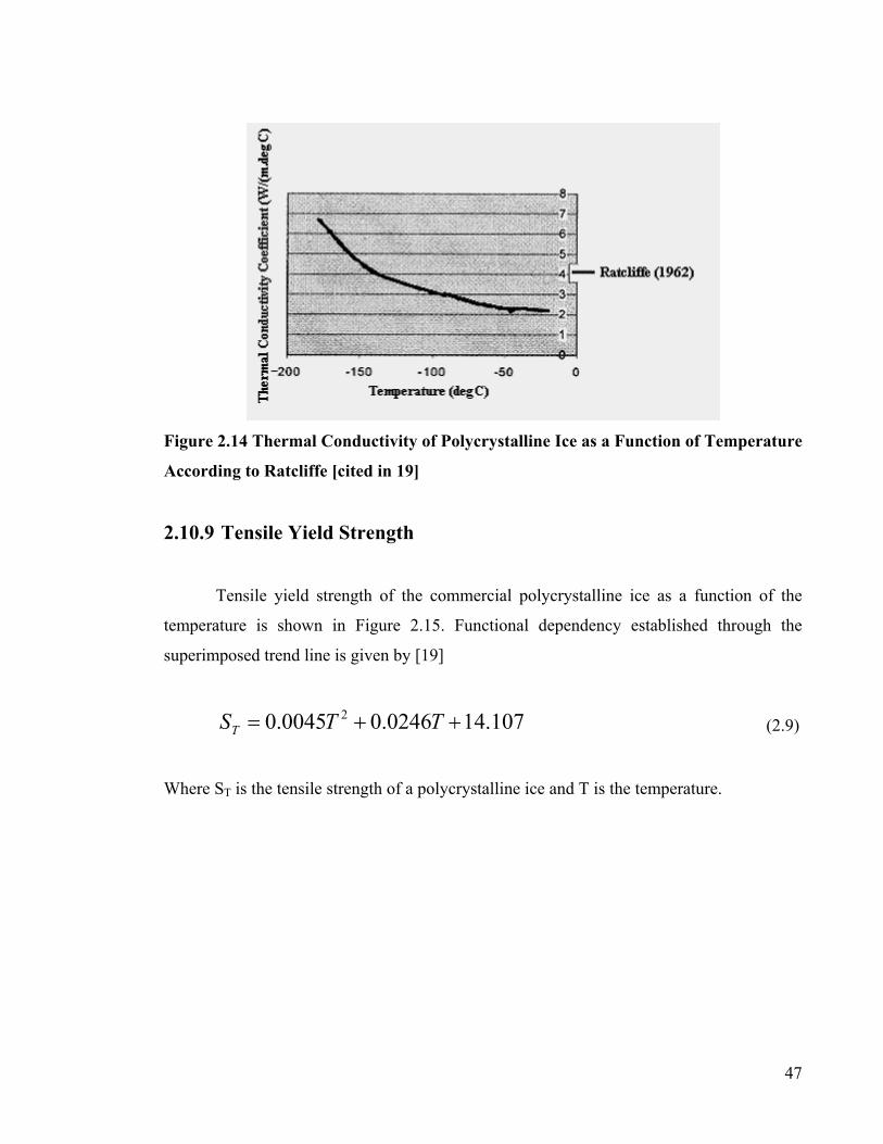
Figure 2.14 Thermal Conductivity of Polycrystalline Ice as a Function of Temperature

According to Ratcliffe [cited in 19]

2.10.9 Tensile Yield Strength

Tensile yield strength of the commercial polycrystalline ice as a function of the

temperature is shown in Figure 2.15. Functional dependency established through the

superimposed trend line is given by [19]

107.140246.00045.0 2 ++= TTST (2.9)

Where ST is the tensile strength of a polycrystalline ice and T is the temperature.

47

Figure

[Butkov

2.11

T

literatur

for this

T

in the

technolo

brittle m

technolo

extent o

quantita

that mig

2.15 Tensile Strength of Polycrystalline Ice as a Function of Temperature

ich]

Summary

he properties and behavior of ice crystals at various temperatures reported in

e has been summarized. The physical and thermal properties of ice are important

study because they indicate the practicability of the current approach

he literature review gives a summary of studies undertaken by various researchers

field of jetting technologies. It discusses the applicability of these existing

gies in the field of cleaning, blasting, surface processing and cutting of ductile and

aterials. Their limitations were presented and discussed in the context of Ice Jet

gy. Most of the researches were concentrated on qualitative experimentation on the

f Ice Jet process on different applications. Although few researches focused on the

tive study, there is still a lack of good understanding of many important parameters

ht pave way for an improvement in methodology used in the Ice Jet process.

48

49

Chapter 3

Design and Development of Ice Jet System

3.1 Introduction

In this chapter the design criteria of the Ice Jet system is addressed. There are

four aspects to be considered:

• Selection of atomizer,

• Design of ice slurry heat exchanger system,

• Design of ice slurry transportation system and

• Design of ice jet cleaning nozzle

The project is aimed to develop a convective heat-transfer heat-exchange system

with both source and sink flowing in the same direction in order to produce ice slurry.

This ice slurry is then transported to the cleaning nozzle. Therefore, the designs of these

systems (atomizer, ice slurry transportation system and cleaning nozzle) are interrelated.

Therefore they are designed in a systematic way using a step by step procedure.

As the aim is to produce ice particles and use them for cleaning under laboratory

conditions, the design and development was carried out with a view to produce less

quantity of ice particles with low velocity. Following sections explain the design and

fabrication of these systems.

3.2 Selection of Atomizer

The first consideration was concentrated on the selection of a suitable atomizer

that is compatible with the required standards of the proposed ice slurry production.

Currently, there are several types of atomizers on the market and the selection of one

depends purely on the purpose to be used. These are conventional spraying nozzles,

50

pneumatic atomizing nozzles and ultrasonic atomizing nozzles. It is also desirable to

know the basic operating functions of these atomizers.

The first and the foremost task was to analyze the working principle, the

advantages, disadvantages and the characteristics of all atomizers. The second task was

to integrate it with the heat exchanger.

There are several characteristics to be studied:

• The volume of water atomized

• The physical size of the water droplets that can be formed from the atomizer

• The temperature range in which the atomizer can operate

• The uniformity of the water droplets formed

• The design compatibility of the atomizer for heat exchanger operations

• The cost factor

In this case the velocity of atomization required should be kept as minimum as

possible to allow most heat transfer to take place between the cryogenic nitrogen and

water droplets.

3.2.1 Water Sprayer

In the first case, a simple operating spraying nozzle was considered for the heat

exchanger needs. A conventional manual sprayer has a tank filled with water and a lever

operated manual pump. By manually operating the lever, pressurized air was supplied

into the liquid tank which increases the air pressure in the tank. When the pressure in

the tank has increased sufficiently, an on/off valve for the spray nozzle was opened to

spray liquid in the tank through a nozzle under the tank air pressure.

As the liquid was discharged, the air pressure in the tank decreases. When the air

pressure drops below a predetermined level, it was impossible to spray liquid with

sufficient momentum. Thus, before the air pressure drops below a predetermined level,

the manual lever had to be operated again to increase the air pressure. Figure 3.1 shows

the front view of the sprayer.

1 Grip 2 Lever 3 Air Tank 4 Brackets 5 Spray Nozzle 6 Air Supply 7 Water Supply

Figure 3.1 Front View of the Sprayer [90] 3.2.2 Pneumatic Atomizer

The design of pneumatic atomizer consists of a pressure chamber for the gas.

The atomization system requires delivery of the liquid to be atomized and the gas to be

used in the resulting spray. Both have to be fed at a rate ensuring that the system lies

within a stable parameter window. Gas and liquid can be dispensed by any type of

continuous delivery system, usually a compressor for the former and a volumetric pump

for the latter. As the liquid gets in contact with the gas the liquid is atomized. The size

of the particle can be controlled by controlling the flow rate of the gas. As the flow rate

of the gas is increased the size of the water droplet decreases, and as the flow rate is

decreased the size of the water droplet increases.

Since the air is fed from the compressor and the velocity of the atomization was

too high, therefore, the use of pneumatic atomizer was not considered for the current

application. Figure 3.2 shows the diagram of pneumatic atomizer.

51

1 Feeding Nozzle 2 Water to be atomized 3 Pressure hamber 4 Orifice f r Gas inlet 5 End of t

nozzle 6 Outlet o7 Atomiza

Figure 3. 3.2.3 U

Th

droplets b

piezo-cera

After amp

There, a

capillary

off into p

means of

liquid was

probe (no

atomized

Co

produce a

droplets g

supply an

ml/sec. H

economic

Co
he feeding
f the Orifice te

2 Schematic Depiction of Pneumatic Atomizer [91]

ltrasonic Atomizer

e third atomizer considered was the ultrasonic atomizer. This produces water

y the acoustic vibration generated with a vibrating assembly. With the aid of

mic elements mechanical oscillations were generated from electric waves.

lifying, these mechanical oscillations were transmitted to the actual atomizer.

liquid film with a defined thickness of layer was incited to produce finest

waves, from the peaks of which fine drop particles were detached and hurled

arabolically shaped trajectories. An appropriate liquid film was obtained by

uniform distribution of the liquid to the atomizer’s surfaces, whereby the

supplied without high pressure. The liquid can be dispensed to the atomizing

zzle) by either gravity feed or a small low-pressure metering pump, and

continuously or intermittently.

ntrary to conventional pressure atomizers, ultrasonic atomizers do not

n increase of speed by means of pressure drop. The outlet speed of the

enerated on the surface of the oscillating body depends on amplitudes, liquid

d water flow rates. The amount of material atomized can be as little as 0.2

ence, this atomization velocity is limited for the aspects of material and

application.

52

Ultrasonic atomizers have very low energy cost, since liquid is supplied without

pressure. These are at higher operating safety, since the atomizer is practically non-

clogging. The diagram of the ultrasonic atomizer is shown in Figure 3.3.

53

Figure 3.3 Ultrasonic Atomizer Model VC 130 AT with Flat Probe

Taking the factors, uniformity of atomization, the range of operating water flow

rate, the range of atomization velocity and the range of operating temperature into

consideration, the ultrasonic atomizer was considered as a better option to atomize

water droplets. It is also considered due to the fact that no other medium for acceleration

or cascade breaking to form water droplets is required.

3.2.4 Calibration of Droplet Size

The selected ultrasonic atomizer has a median drop size ranging from 80 to 120

microns with the frequency of 40 KHz. This was calibrated with a Phase Doppler

Particle Analyzer (PDPA). The limitation of the PDPA model used for this purpose was

0.5 microns at the lower end and 5 mm at the upper end.

3.2.5 Operating Principle of PDPA

The Phase Doppler Method is based upon the principles of light scattering

interferometry and is shown in Figure 3.4. Measurements were made at a small, non-

intrusive optical probe volume defined by the intersection of two laser beams. The

intersection of the two beams creates a fringe pattern within the probe volume. As a

particle passes through the probe volume, it scatters light from the beams and projects

the fringe pattern. A receiving lens located at an off-axis collection angle projects a

portion of this fringe pattern onto several detectors. Each detector produces a Doppler

burst signal with a frequency proportional to the particle velocity. The phase shift

between the Doppler burst signals from two different detectors is proportional to the

size of the spherical particles. This chapter only discusses the calibration of atomized

water droplets. Figure 3.4 shows the operating principle of PDPA.

Source: Kenelec Scientific

Figure 3.4 Operating Principle of PDPA

3.2.6 Selection of Atomizer probe

The atomizer probes selected can produce uniform flow rates, ranging from 1

lit/hr to 12 lit/hr. Two types of probes were used in order to vary the inlet flow rate. The

two probes selected for this ultrasonic atomizer model are shown in Figure 3.5. Figure

3.6 shows the flat probe atomizing the water droplets.

It was verified experimentally that the probe can operate at very low

temperature. This is due to the fact that the atomization was carried out by ultrasonic

vibrations and practically the vibrations unclog any blockage at the probe tip. The

experimental details are given in Chapter 6.

54

67m

118

65mm

36mm

a) b)

Figure 3.5 a) Flat Tip Half Wave Medium Atomization Rate (200ml/min) and b) Flat Tip Half Wave Low Atomization Rate (60ml/min)

Figure 3.6 Flat Probe Atomizing the Water Droplets

3.3 Design of Heat Exchanger

There are various types of heat exchanger designs available for applications.

They can generally be classified as parallel flow, counter flow and cross flow heat

exchangers. However, in this study the focus is on designing a Parallel Flow Direct

Contact Heat Exchanger by convective heat transfer mechanism. The reason for this is

to facilitate the ice particle to flow along with the carrier gas to maximize heat transfer.

As the velocity of the droplets generated was low, the probe of the atomizer was 55

mounted with the tip facing downwards and therefore the design of the heat exchanger

was considered vertical. The cryogenic nitrogen was injected from the top due to its

property of being heavier than air and therefore flows downwards. Thus in order to

design it, necessary parameters such as length, diameter, its surface area and the

material were calculated. This calculation was dependent on the water droplet velocity,

diameter, dispersion area and cryogenic nitrogen temperature, velocity and mass flow

rate.

As the atomized water droplets were very small, in the order of microns the

lumped capacitance model was used to find out the length of the heat exchanger [92].

This is explained in the next subsection.

3.3.1 Lumped capacitance method This method is based on the following assumptions:

• The water droplets are spherical

• The water droplets are atomized at a uniform and constant temperature

• The temperature inside the droplet remains uniform and changes with time

• Cryogenic nitrogen is assumed to be at uniform temperature An energy balance of the droplet for the time interval, dt, can be expressed as follows. Heat transfer into the body during, dt = the increase in the energy of the body during, dt i.e., (3.1) dTmCdtTThA ps =−∞ )( This can be rearranged as

dtVChA

TTTTd

p

s

ρ−

=−−

∞

∞ )( (3.2)

Integrating from t = 0, at which T =Ti, to any time t, at which T=T(t), gives

tVChA

TTTtT

p

s

i ρ−=

−−

∞

∞)(ln (3.3)

56

And therefore,

∞

∞

−−

−=TTTtT

hAVC

tis

p )(lnρ

(3.4)

Where the convective heat transfer coefficient, h, is,

6.0

37.0⎥⎥⎦

⎤

⎢⎢⎣

⎡= ∞

f

f

vdu

dK

h (3.5)

After obtaining the temperature T(t) at time t, the rate of convection heat transfer

between the droplet and the surrounding atmospheric air was obtained by Newton’s law

of cooling as

])([)( ∞−= TtThAtQ s (3.6)

But as the water droplet is moving with respect to time t, the problem was considered

transient. The time taken to form ice particles was calculated from the equation,

S = Ut +1/2 gt2.

As the nitrogen and water droplets are flowing in the same direction, it was assumed

that there was no counter viscous drag opposing the flow of water droplets. As the water

droplets have an initial velocity >0 and accelerates due to gravity the Newton’s law was

used in calculating the distance. The length was calculated based on the time taken for

the droplets to convert ice particles. However, the design was “under surfaced” in order

to obtain a difference in temperature between ice particles and cryogenic nitrogen. The

extent of “under surface” is given in Chapter 6

3.3.2 Heat Exchanger Diameter

Diameter of the heat exchanger was found out by the Nozzle discharge pattern

of the ultrasonic atomizer’s probe. This was calculated through experimental

measurements of the actual pattern. The discharge angle and the diameter of the actual

spray were calculated to find out the diameter and shape of the heat exchanger. Figures

3.7 and 3.8 visualize atomization of water droplets for different water flow rate and

57

atomization. The largest discharge angle was obtained for 200ml/min with the

amplitude of 100.

a) Figure 3.7 a) Water Flow Rate of 1 l/hr at th b) Water Flow Rate of 6 l/hr at th

a) Figure 3.8 a) Water Flow Rate of 12 l/hr and Am b) Equalized Contract of the Atomized

b)

e Amplitude of 40 and e Amplitude of 80

b) plitude of 100, and

Water Droplets Pattern

58

The atomization pattern can be expressed with an illustration as shown in Figure 3.9.

Rd

Φ

θ

Figure 3.9 Illustration of the Discharge Angle, the Discharge Diameter and the Atomized Droplets (Φ = Curvature expressing the energy loss of the atomized water droplets, θ = discharged angle, Rd = discharge radius)

As the discharge radius (function of water flow rate and atomization) increases

the rate of droplets energy loss increases. In this chapter, the study is limited to find out

the discharge angle and discharge radius only. Therefore, the diameter of the heat

exchanger was calculated on the basis of the discharge radius with tolerance given

through the inner surface as per the TEMA regulations [93]. More details of the heat

transfer phenomenon are described in Chapters 6 and 7.

As the heat exchanger built has to operate under very low temperature, it was

necessary to analyze the material and thermal properties. For that, the design was

initially built using Pro/Engineer and the Finite Element Analysis was carried out using

Pro/Mechanica Structure and Thermal modules. This was done to select the material,

thickness of walls, the amount of insulation used and to select the constraint surface.

The 3-D model of the heat exchanger is shown in Figure 3.10. A shell model was drawn

59

instead of a solid model to analyze the distribution of temperature, stress-strain and the

displacement-magnitude on the walls.

Cryogenic Nitrogen Inlet

Atomized Water Inlet

Ice particle, Air & Nitrogen Outlet

Air supply unit

Figure 3.10 3-D Shell Model of the Heat Exchanger showing Finite Elements

The exact design drawings of the heat exchanger and the air supply unit are given in

Appendix B. The material properties for the selected design are given in Table 3.1

Table 3.1 Material Properties of Aluminum

Properties Values

Units

Mass Density 2.794 x 10-9

Kg/m3

Young’s Modulus

7.3080 x 104

N/m2

Poisson’s Ratio 0.33

Coefficient of Thermal Expansion 2.304x 10-5

W/°Cm2

A range of thermal properties were selected for the analysis which are given in Table 3.2 60

61

Table 3.2 Thermal Properties of Aluminum

Properties

Values

Units

Convective Coefficient 2 to 10

W/°Cm2

Bulk Temperature

10 to 20

°C

Cryogenic Nitrogen Temperature -50 to -140 °C

In using the Pro/Mechanica for thermal analysis there are certain procedure to be

followed. It is an iterative process where by different values of the parameters were

given and tested. Optimization of this process was an important issue and was obtained

by using a range of both material and thermal properties.

The wall temperature, Displacement-Magnitude and the Stress-Strain plots of

the heat exchanger are shown in Figures 3.11, 3.12 and 3.13.

The Figure 3.11 shows that the minimum temperature of the wall at the entry

point of the heat exchanger was -9°C with the cryogenic nitrogen flowing at -120°C.

The Figure 3.12 shows that the maximum structural displacement using the analysis was

0.8mm at the cryogenic nitrogen entrance, but in general it varied from 0.1mm to

0.3mm on an average.

Finally the Von-Mises stress was analyzed and is shown in Figure 3.13. The

maximum stress was concentrated on the top surface of the heat exchanger with the

values ranging from 213 N/m2 to 60 N/m2. But, in the rest of the heat exchanger area the

average value was 30 N/m2.

Figure 3.11 Temperature Distribution of Heat Exchanger

Figure 3.12 Displacement-Magnitude of the Heat Exchanger

62

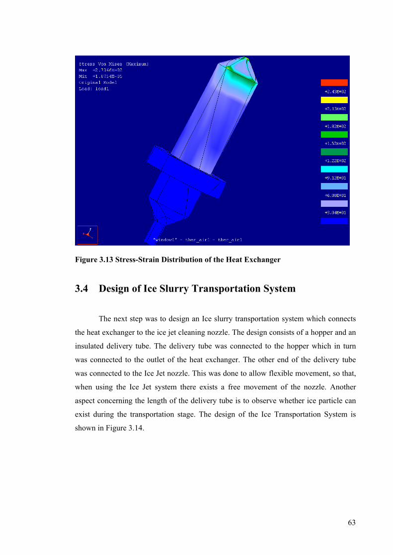
Figure 3.13 Stress-Strain Distribution of the Heat Exchanger

3.4 Design of Ice Slurry Transportation System

The next step was to design an Ice slurry transportation system which connects

the heat exchanger to the ice jet cleaning nozzle. The design consists of a hopper and an

insulated delivery tube. The delivery tube was connected to the hopper which in turn

was connected to the outlet of the heat exchanger. The other end of the delivery tube

was connected to the Ice Jet nozzle. This was done to allow flexible movement, so that,

when using the Ice Jet system there exists a free movement of the nozzle. Another

aspect concerning the length of the delivery tube is to observe whether ice particle can

exist during the transportation stage. The design of the Ice Transportation System is

shown in Figure 3.14.

63

Hopper

Delivery Tube

a) b) Figure 3.14 a) and b) Start and End Section of the Ice Slurry Transport System in 3-D Model with the Datum Planes

3.5 Design of Ice Jet Cleaning Nozzle

The existing abrasive jet nozzle at IRIS was taken as the basis for modeling the

Ice Jet Nozzle. A simple model of the Ice Jet cleaning nozzle is shown in Figure 3.15.

The delivery tube was attached to the Ice particle feed which forms the part of the

nozzle design. The nozzle is also comprised of a focus tube in which the ice particles

are accelerated by either pressurized air or water depending on the velocity

requirements. The detailed process inside the nozzle is described in Chapter 7.

64

Inlet for Ice/Water

Ice particle feed

Focus Tube

Figure 3.15 Design of Ice Jet Nozzle with the Focus Tube In summary, the components that constitute the entire Ice Jet system were designed.

However, more emphasis was given to the design of heat exchanger as that was the

main component to produce ice particles. The heat exchanger was then fabricated and

experiments were carried out to study the ice particle formation.

65

66

Chapter 4

Experimental Setup and Procedure 4.1 Overview

As discussed in the preceding Chapters, the main objectives of this research

investigation were to study the feasibility of ice particle formation using a custom built heat

exchanger and to verify the results of a numerically built model with that of the

experiments. Further, a numerical model will be developed to study the effects of ice

particles through the transportation stage and inside the Ice Jet nozzle.

To this end, a full factorial design is developed and the parameters, cryogenic

nitrogen temperature, cryogenic nitrogen flow rate, inlet water temperature, water droplet

diameter (function of atomization rate) and the water flow rate are varied within practical

ranges. Visualization experiments are also conducted which could help in understanding

further the behavior and characteristics of ice particles flowing out of the heat exchanger.

This chapter describes the experimental setup and procedures of Ice particle formation

process using the heat exchanger. The following sections focus in describing the ice particle

formation process. Specific details of the experiments as well as the methodology used in

carrying out these experiments are presented.

4.2 Ice Particle Formation Process

A schematic diagram of the experimental process for ice particle production is

shown in Figure 4.1. The experimental setup consists of a heat exchanger system, an

ultrasonic atomizing unit, a liquid nitrogen storage unit, a water storage unit, a chilling unit

and an air compression unit.

The heat exchanger was the main unit which was connected to the liquid nitrogen

storage unit and the ultrasonic atomizing unit. The ultrasonic atomizing unit was connected

to a water storage unit which in turn was connected to a chiller. Initially there existed a

clogging problem because of the ice particles sticking to the walls and slowly building up

and blocking the outlet. Therefore, to rectify this problem an air compression unit was also

connected to the heat exchanger through two inlets as shown in Figure 4.1. This unit

introduces an air cushion on to the inner surface of the heat exchanger thus preventing the

ice particles sticking to the walls.

67

Figure 4.1 Schematic of the Ice Slurry Formation Process and Temperature Measurement System

In order to make water freeze effectively it was important to reduce the heat

incoming to the water from its surroundings. Therefore, the heat exchanger was insulated to

minimize the heat transfer. The heat exchanger was built in such a way that there is

effective heat transfer between the cryogenic nitrogen and the water droplets.

Thermocouple 1 Water Storage

Chiller

Ultrasonic Atomizer

Heat Exchanger

Thermocouple 2

Liquid Nitrogen Storage Unit

Data Acquisition System

1 Thermocouple reading of the inlet Cryogenic nitrogen temperature

Thermocouple Locations:

2 Thermo couple reading of the exit cryogenic nitrogen temperature

3 & 4 Thermocouple readings of the outlet ice particles temperature

Data Logger

Thermocouple 3 & 4

Ice slurry collector

Air Compressor unit

68

Water from the water storage unit is filtered and fed into the ultrasonic atomizer’s

probe. Water flowing to the atomizer was pre-cooled to the desired temperature through a

chilling unit. Liquid nitrogen was stored under pressure in the storage unit and was

transferred to the heat exchanger through a transfer tube. Two air inlets were provided near

the exit of the heat exchanger to control the flow of ice particles. One of the inlets is for the

air to travel in an upward direction and the other to travel in a downwards direction,

uniformly through the inner surface of the heat exchanger. Air from the compressor was fed

into these inlets and the pressure regulated to provide a smooth cushioning effect inside the

heat exchanger. Another effect of the air is to accelerate ice particles through the ice

particle transport system. An insulated ice particle collector was used to collect the ice

particles at that stage of the experiment.

K-type thermocouples were used to measure temperature at various points of the

heat transfer process as shown in Figure 4.1. The thermocouples were connected to a data

acquisition system which in turn was connected to a computer. These thermocouples read

the online variation of cryogenic nitrogen temperature at the inlet and outlet of heat

exchanger and the temperature of ice particles inside the ice particle collector. The time

interval for each reading was controlled using a real time operating software, which also

has a real time display of the temperature variation of all the thermocouples. A distance was

provided between the thermocouples and the bottom plane of the collector. This was done

to measure the temperature of flowing ice particles and not the already deposited particles.

Readings were taken with all thermocouples until the ice particle temperature exiting the

heat exchanger stabilized.

4.3 Measuring Devices and Accuracy Assessment 4.3.1 Thermocouple

In order to measure the cryogenic nitrogen temperatures, a thermocouple capable of

measuring very low temperature was selected. Type K is a general purpose thermocouple

with a measuring range of -200°C to +1200°C. The sensitivity is approx 41µV/°C. A data

69

logger capable of measuring K-type thermocouples was also selected. These thermocouples

have an accuracy of ± 1°C.

4.3.2 Cryogenic Nitrogen Flow Rate Measurements

It is highly desirable to measure the flow rate of the cryogenic liquid/gas nitrogen

flowing out of the heat exchanger. Because of the two-phase flow of the cryogenic nitrogen

the measurement was highly expensive and was beyond the laboratory experimental

measurement conditions. Therefore, the specifications were obtained from British Oxygen

Company (BOC), the company which supplied liquid nitrogen for the experiments. The

specifications involved the flow rate calibrated against the pressure regulator and the

opening valve. However, there are few published research reports on the measurements of

cryogenic nitrogen flow rate [94].

4.3.3 Water Flow Meter

In order to measure the flow rate of water a flow meter capable of measuring all

experimental flow rate range was selected. The selected flow meter has an error of ±2%

4.3.4 Inlet Tube Angle of Nitrogen

This was required to regulate the point of contact between nitrogen and water

droplets. A special stand was made and the inlet tube angle measured using a protractor.

The error obtained by this measurement was about ±1%

The atomizer has an error of + 100Hz for the 40 KHz model used in this experiment

The total experimental uncertainty was calculated to be ±5%, which is the addition of the

total measurement error.

70

4.4 Design of Experiments

Initially a complete randomized design of experiments was conducted in order to

determine the appropriate range of the parameters to obtain the ice particles from the heat

exchanger. In conducting these experiments, the predictor variables used were the

cryogenic nitrogen temperature, flow rate, angle of nitrogen inlet into heat exchanger, water

temperature, flow rate and atomization rate. The response or dependent variables were the

outlet ice particle and cryogenic nitrogen temperature.

A total number of runs was calculated with a full factorial design. These required 54

runs, with complete repeat to measure the outlet ice particle temperature. Because of

randomization the run order was considered to minimize the effects of other factors that

were not included in the study. The ranges of operating parameters used in all these

experiments are shown in Table 4.1.

Table 4.1 Initial Range of Experimental Parameters

Cryogenic Nitrogen Temperature °C -100, -120 Nitrogen Flow Rate l/min 0.5, 1.0, 1.5 Inlet Angle degrees 15, 30, 45, 60 Inlet Water Temperature °C 5, 10, 15 Water Flow Rate l/min 0.03, 0.1, 0.2 Droplet diameter µm 80, 100, 120 Air temperature °C 10, 20 Air flow rate l/min 0.25, 0.5, 0.75

The number of predictor parameters used was brought down to smaller ranges. In

most of the experiments an optimal angle of 30° for the inlet nitrogen was used and the

details of which are discussed in Chapter 6. The inlet water flow rate was kept at the

maximum of 0.2 kg/min and only the atomization rate varied to vary the droplet diameter.

Regression and allied techniques were used to analyze the data and obtain a best fit curve.

4.5 Visualization Experiments

Figure 4.2 shows the schematic diagram of the visualization process used to conduct

experiments in this project. A camera capable of capturing 120 frames/seconds at full

resolution (648 x 484 pixels) was connected to a computer and the images stored for further

processing. The camera was placed under the heat exchanger just at the outlet and the ice

particles flowing out recorded. A black background was placed in order to capture a clear

view of the ice particles. The recorded images were later analyzed using image analysis

software.

71

Figure 4.2 Schematic of the Ice Slurry Formation Process with Camera Attached for Visualization Study

Table 4.2 shows the ranges of operating parameters used in the visualization

experiments conducted to study the behavior of ice particles at different exit temperatures.

Most of the parameters were kept constant except the cryogenic nitrogen temperature and

the droplet diameter. This was done to observe the mixture of ice/water droplets and efforts

Water Storage

Chiller

Ultrasonic Atomizer

Heat Exchanger

Liquid Nitrogen Storage Unit

High-Speed Camera

Ice slurry collector

were also made to study the phenomenon of ice particle freezing. The change in ice particle

diameter with the initial water droplet diameter was also studied.

Table 4.2 Range of Parameters for Visualization Experiments

Cryogenic Nitrogen Temperature °C -120 Nitrogen Flow rate l/min 1.5 Inlet Angle degrees 30 Inlet Water Temperature °C 5 Water Flow Rate l/min 0.2 Droplet diameter µm 120 Air temperature °C 10 Air flow rate l/min 0.5

The components used in visualization experiments and analysis consisted of two

major groups, which were the Video Capture system and the Image Analysis Software. The

Video Capture System included a PULNIX TM-6710 high resolution progressive scan

monochrome camera with non-interlace quad speed scanning shown in Figure 4.3 and an

Inspecta 4 Video Capture Card, and its software. The image analysis used for visualization

experiments was V++, and various in-house scripts were developed to enhance and

automate some of the tasks involved such as capturing the successive trace of the ice

particles falling from the heat exchanger.

Figure 4.3 PULNIX TVisualization Experim

M-6710 High Resolution Progressive Scan Camera Used in the ents

72

The camera was protected from ice particles and the exiting cryogenic nitrogen by

enclosing it in a protective casing. A long video cable was used to connect the camera to a

dedicated computer that was used to download and store images of the traces of falling ice

particles. A large RAM was used to store the data before writing it on to the hard disk.

Figure 4.4 shows the attachments and accessories used to produce ice particles in the Water

Jet lab at IRIS.

Figu

reso

shut

re 4.4 Attachments and Accessories of the Ice Jet System

The high-speed camera was capable of recording up to 120 frames per second at full

lution, 648(H) X 484(V) pixels, up to 300 frames at partial resolutions with frame

ter speeds of 1/60 to 1/32,000 second. However, acquiring images at high speeds

73

74

generates a high volume of data that need to be stored in the hard disk for further analysis.

In addition, data write to the hard disk is much slower than the rate of data generation.

Therefore, a very large RAM needs to be used as buffer storage for the data before it could

finally be written on to the hard disk for permanent storage.

The camera frame rate that was used in this project to acquire the images was 120

frames per second. This rate was chosen because in addition to the problem with writing

and storing the data, an image acquisition at a higher frame rate than 120 frames per second

does not give better performance, as some of the images that were captured in successive

frames at higher frame rate were identical.

To summarize, in this chapter, the experimental procedures, the measuring

equipments and the design of experiments are detailed and the results of the experiments

are discussed in Chapter 6. Based on the experiments range of parameters, CFD simulations

were also predicted, of which the procedures and governing equations are explained in

Chapter 5.

Chapter 5

Modeling of Ice Jet Process

5.1 Introduction

This chapter develops the subject of modeling and computational heat transfer of ice

jet process by relating the available numerical procedures to the solution of differential

equations, governing heat transfer processes. The nature of equations relevant to the study

of heat transfer of dispersed particles into a cold gas is discussed in terms of both

differential and integral formulations. The appropriate boundary conditions are given with

finite volume approach. Various discretization formulations are outlined, along with the

associated errors, convergence characteristics and numerical stability.

The heat transfer process of conduction, convection and radiation are dealt within

practical ranges to investigate the temperature distribution inside the heat exchanger,

transportation system and Ice Jet focus tube. The numerical analysis was carried out using

CFX, a Computational Fluid Dynamic (CFD) package.

5.2 Problem Definition in Modeling

The numerical approach of the entire Ice Jet system was categorized into three sections:

1. Heat transfer inside heat exchanger

2. Heat transfer inside transportation system

3. Heat transfer inside Ice Jet focus tube

In all sections the heat transfer equations under conduction, convection and radiation

were used along with inter-phase heat and momentum transfer, inter-phase drag, overall

and specific heat transfer and thermal phase change problem with latent heat. However, the

75

major difference in solving the heat transfer inside the focus tube is that the flow was

considered turbulent as opposed to the flow in heat exchanger and transportation system,

where the flow was considered laminar. The turbulence inside the focus tube is due to a

high Reynolds number pertaining to high velocity and high pressure water/air, used to

accelerate the ice particles.

5.2.1 Heat Transfer Inside Heat Exchanger

The temperature distribution of freezing droplets is of major importance to study the

effect of surface area of the designed heat exchanger. However, as described in the previous

chapters it is simply described as the solidification of liquid by atomization into a cold

atmosphere. Being able to determine the temperature at different planes would effectively

optimize the heat exchanger design. A diagram showing the droplets dispersing inside a

cold atmosphere is given in Figure 5.1

Cryogenic Nitrogen Gas (Continuous Phase)

Figure 5.1 Droplets Dispersed by an AOver it

Atomizer

Droplets (Dispersed Phase)

tomizer with Cryogenic Nitrogen Gas Flowing

76

Here water droplets were considered as dispersed phase while cryogenic nitrogen

was considered as continuous phase. Disperse phase flows are flows in which one phase is

not materially connected.

To predict the experimental results it was important to set those exact conditions in

modeling. To do that an air inlet was introduced on the lower block and projected vertically

downwards throughout the inner surface of the heat exchanger. This constituted a third

phase to be considered for the heat transfer. The illustration of this is given in Figure 5.2.

Air Inlet System Air Inlet

Air flowing through the inner surface and downwards

Figure 5.2 Introduction of Air Inlet System on the Lower Block of the Heat Exchanger

77

5.2.2 Ice Slurry Transportation System

In defining this system there exist heat transfer among nitrogen, air and water/ice

particles. But unlike three inlets for the heat exchanger, in this system there is only one inlet

for all the phases to flow through. Figure 5.3 shows the representation of the transportation

system. The droplets are treated as dispersed phase and the air and nitrogen as continuous

phase. The single particle equations for the heat and momentum transfer used for the heat

exchanger were also used in transportation system. The set of equations is given in Section

5.4 and is discretized by finite volume approach.

Ice Particles

Cryogenic Nitrogen Air Figure 5.3 Schematic of the Representation of Transportation System

The flow inside the transportation system was considered laminar owing to the low

Reynolds number. The effect of air velocity and nitrogen temperature on the ice particles is

discussed in Chapter 6.

78

5.2.3 Ice Jet Nozzle

The heat and momentum transfer was considered to occur among air/water, nitrogen

and dispersed ice particles. The equations of heat and momentum transfers are given in

Section 5.4. Eulerian-Eulerian model was used with turbulent flow k-ε equations. Figure

5.4 shows the representation of the ice jet nozzle.

Air/Water

Ice particles

Air +Nitrogen

Figure 5.4 Representation of Different Inlet and Phase Inside the Nozzle The basic definitions of the terminologies are detailed in Appendix A. 5.3 Hypothesis

A laminar flow, continuous-dispersed, inter-phase model was selected. Particle

model involving Eulerian-Eulerian multi phase model was used for the inter phase heat

transfer. Thermal phase change model was considered owing to the latent heat phase

79

transformation of water droplets to ice particles. The assumptions used for these models are

as follows.

• Droplets remain spherical

• Water droplets were assumed as dispersed phase, cryogenic nitrogen and air were

considered as continuous phase

• Ice particles were formed by latent heat transfer between cryogenic nitrogen and

water droplets

• Conduction inside the droplets was assumed to be instantaneous as droplet diameter

is approximately 100µm. This is based on the analytic solution of transient heat

conduction inside a solid sphere [95]. It assumes that advection effects inside the

drop may be neglected and the time-dependent temperature field inside the sphere

may be considered to be spatially constant.

• No droplet coalescence occurs

• Eulerian-Eulerian method was used because of higher convergence rate

• A forward difference time discretization was used to solve the transient droplet

temperature

The governing equations of inter-phase heat transfer, interfacial area density, the drag

coefficient and the heat balance for the total mass flux are discussed in detail.

5.4 Governing Equations 5.4.1 Interfacial Area Density

Interfacial transfer of momentum, heat and mass is directly dependent on the contact

surface area between the two phases. This was characterized by the interfacial area per unit

volume between phase α and phase β , known as the interfacial area density .

Interfacial area density has dimension of one over length and in this problem was modeled

using the Particle model.

αβA

80

5.4.1.1 Particle Model

The particle model for interfacial transfer between two phases assumes that one of

the phases is continuous (phase α) and the other is dispersed (phase β). The surface area per

unit volume is then calculated by assuming that phase β is present as spherical particles of

mean diameter, dβ. Using this model, the inter-phase contact area is given by

βαβ

βdrA 6

= (5.1)

Non-dimensional, inter-phase transfer coefficients may be correlated in terms of the

particle Reynolds number and the fluid Prandtl number. These are defined using the particle

mean diameter, and the continuous phase properties, and are given by

α

βαβααβ µ

ρ dUU −=Re (5.2)

α

αααβ λ

µ PC=Pr (5.3)

where, ααα µρ PC,, and αλ are the density, viscosity, specific heat capacity and thermal

conductivity of the continuous phase α respectively.

5.4.2 Inter-Phase Heat Transfer

In the multiphase model, there are separate enthalpy and temperature fields for each

phase. Heat transfer is governed by the multiphase thermal energy equations for sensible

enthalpy (incompressible and low speed compressible flows only) and therefore the

Equation 5.4 can be used as transportation equation:

( ) ( )( )Υ αααααααα λρ ρ Thrhrt

∇−×∇+∂∂

= (5.4) ∑=

++ ++Γ−ΓNp

ss SQhh1

)(β

αααβαβαβ

where

81

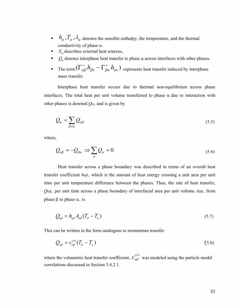
ααα λ,,Th denotes the sensible enthalpy, the temperature, and the thermal conductivity of phase α.

describes external heat sources, αS denotes interphase heat transfer to phase α across interfaces with other phases. αQ

The term represents heat transfer induced by interphase mass transfer.

)( ss hh αβαβαβ++ Γ−Γ

Interphase heat transfer occurs due to thermal non-equilibrium across phase

interfaces. The total heat per unit volume transferred to phase α due to interaction with

other phases is denoted Qα, and is given by

αβαβ

α QQ ∑≠

= (5.5)

where,

0=⇒−= ∑ αα

βααβ QQQ (5.6)

Heat transfer across a phase boundary was described in terms of an overall heat

transfer coefficient hαβ, which is the amount of heat energy crossing a unit area per unit

time per unit temperature difference between the phases. Thus, the rate of heat transfer,

Qαβ, per unit time across a phase boundary of interfacial area per unit volume Aαβ, from

phase β to phase α, is

)( αβαβαβαβ TTAhQ −= (5.7) This can be written in the form analogous to momentum transfer

)()(αβαβαβ TTcQ h −= (5.8)

where the volumetric heat transfer coefficient, was modeled using the particle model correlations discussed in Section 5.4.2.1.

)(hcαβ

82

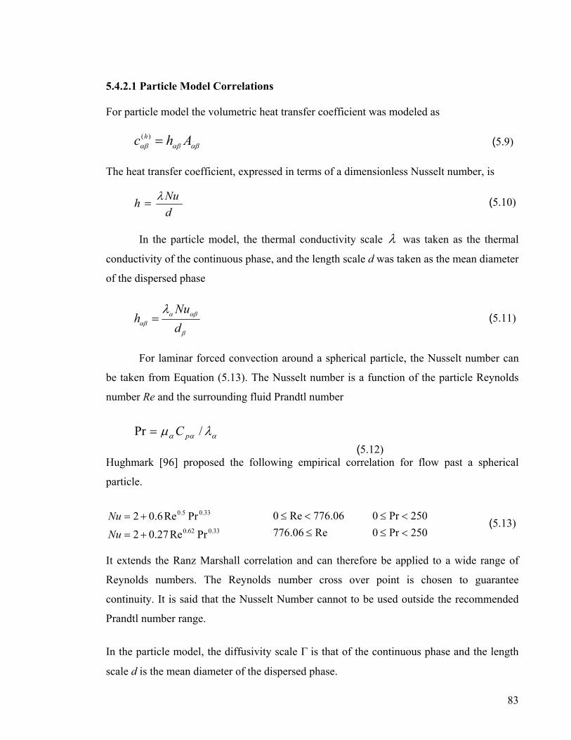
5.4.2.1 Particle Model Correlations For particle model the volumetric heat transfer coefficient was modeled as

αβαβαβ Ahc h =)( (5.9) The heat transfer coefficient, expressed in terms of a dimensionless Nusselt number, is

dNuh λ

= (5.10)

In the particle model, the thermal conductivity scale λ was taken as the thermal

conductivity of the continuous phase, and the length scale d was taken as the mean diameter

of the dispersed phase

β

αβααβ

λdNu

h = (5.11)

For laminar forced convection around a spherical particle, the Nusselt number can

be taken from Equation (5.13). The Nusselt number is a function of the particle Reynolds

number Re and the surrounding fluid Prandtl number

ααα λµ /Pr pC=

(5.12) Hughmark [96] proposed the following empirical correlation for flow past a spherical

particle.

33.062.0

33.05.0

PrRe27.02PrRe6.02

+=

+=

NuNu

Re06.77606.776Re0

≤<≤

250Pr0250Pr0

<≤<≤ (5.13)

It extends the Ranz Marshall correlation and can therefore be applied to a wide range of

Reynolds numbers. The Reynolds number cross over point is chosen to guarantee

continuity. It is said that the Nusselt Number cannot to be used outside the recommended

Prandtl number range.

In the particle model, the diffusivity scale Γ is that of the continuous phase and the length

scale d is the mean diameter of the dispersed phase.

83

β

αβααβτ

dShΓ

= (5.14)

5.4.2.2 Interface Flux

This is implemented in the inter-phase heat transfer models which use a complex

form heat transfer coefficient multiplied by a bulk temperature difference. The heat flux

coefficients for both fluids and the interfacial heat flux value, F12, from cryogenic nitrogen

to water droplets are specified. F12 is the rate of heat transfer per unit time per unit

interfacial area from phase 1 to phase 2. Hence the heat transferred to fluid 2 from fluid 1

per unit volume is given by

12121221 FAQQ =−= (5.15)

F12 may be given as a constant or an expression. Typically, F12 will be a function of the

fluid 1 and fluid 2 temperature fields. In this case, the converge of the coupled solver was

accelerated specifying optional fluid 1 and fluid 2 heat flux coefficients.

,01

121 ≥

∂∂

≈TFh 0

2

212 ≥

∂∂

≈TFh (5.16)

For numerical stability, the values of the coefficients used were positive. The partial

derivatives were not exactly calculated, as it was sufficient for the specified coefficients to

simply approximate the partial derivatives. Specification of heat flux coefficients only

affected the convergence rate to the solution of the coupled heat transfer equations, and did

not affect the accuracy of the converged solution. The model using a heat transfer

coefficient multiplied by a bulk temperature difference is

),( 212112 TThFF −=−= hhh == 21 (5.17)

5.4.3 Thermal Phase Change

As the model assumes latent heat transfer from cryogenic nitrogen to water droplets

to form ice particles, the thermal phase change model was taken into consideration. The

inter-phase heat transfer was used in conjunction with the thermal phase.

84

The Thermal Phase Change Model assumes: • that thermodynamic equilibrium prevails at the interface between the two phases. That is,

the interfacial temperature equals the saturation temperature.

• that heat transfer of both sides of the droplets was modeled by two independent heat

transfer coefficients.

5.4.3.1 Latent Heat This was obtained due to the difference between the static enthalpies of the two phases.

)()( satliquidsatgas THTHL −= (5.18)

Hence, the absolute enthalpies of the two phases were also taken into consideration. The thermal phase change model requires the use of the two resistance model for inter-

phase heat transfer.

5.4.3.2 The Two Resistance Model

It was thought that the use of overall heat transfer coefficient was not sufficient to

model the inter-phase heat transfer process and therefore the resistance model was

incorporated. A more general class of models considers separate heat transfer processes

either side of the phase interface. This was achieved by using two heat transfer coefficients

defined on each side of the phase interface. Defining the sensible heat flux to phase α from

the interface as

)( ααα TThq s −= (5.19)

And the sensible heat flux to phase β from the interface as:

)( βββ TThq s −= (5.20)

where and are the phase α and phase β of heat transfer coefficients respectively. Ts

is the interfacial temperature, and it is assumed to be the same for both phases.

αh βh

85

The fluid-specific Nusselt number is defined as:

α

αβαα λ

dhNu = (5.21)

Where, λα is the thermal conductivity of fluid α, and dαβ is the interfacial length

scale (the mean particle diameter for the Particle Model). However, this model is only valid

where there is no mass transfer. In that case, the interfacial temperature is determined from

the sensible heat balance 0=+ βα qq

In case of Inter Phase Mass Transfer, it is determined by total heat balance, i.e. the total

heat flux to phase α from the interface

sHmqQ ααβαα += (5.22) Total heat flux to phase β from the interface:

sHmqQ βαβββ −= (5.23)

where, denotes mass flux into phase α from phase β, αβm

and, Hαs and Hβs represent interfacial values of enthalpy carried into and out of the

phases due to phase change,

The total heat balance 0=+ βα QQ determines the inter-phase mass flux given by

ss HHqq

mαβ

αβαβαβ −

+= (5.24)

5.4.3.3 Secondary Fluxes

This secondary heat flux term was modified in order to take into account the

discontinuity in static enthalpy due to latent heat between the two phases. This is achieved

using a modification of the upwind formulation (Equation 5.25), by Prakash [97]. In this

formulation, the bulk fluid enthalpy is carried out of the outgoing phase, as in the default

86

upwind formulation. However, the saturation enthalpy is carried into the incoming phase.

Thus, the modified formulation is

)( αβαβαβαβ φφ ++ Γ−Γ=MS (5.25)

ββαααβ HHHHm ssats ==⇒> ,0

satss HHHHm ββαααβ ==⇒< ,0 This leads to a formulation which was stable both physically and numerically. Thereby the

denominator of Equation 5.24 is non-zero, being greater than or equal to the latent heat

satsat HHL αβ −= (5.26)

5.4.4 Inter-Phase Mass Transfer

Interphase mass transfer occurs when mass is carried from one phase into another. It

is applicable to both the inhomogeneous and homogeneous multiphase models. Due to the

phase change it is definite that there is mass transfer.

Mass transfer is represented by sources in the phasic continuity equations and is given by

ααααααα ρρ Γ+=•∇+∂∂ SUrrt

)()( (5.27)

Sα describes user specified mass sources,

Гα is the mass source per unit volume into phase α due to interphase mass transfer.

This is expressed as follows:

αββ

α Γ=Γ ∑=

pN

1 (5.28)

αβΓ is the mass flow rate per unit volume from phase β to phase α.

87

It is assumed that

01

=Γ⇒Γ−=Γ ∑=

αα

βααβ

pN

(5.29)

As it was important to keep track of the direction of mass transfer processes, it is

convenient to express as follows αβΓ

++ Γ−Γ=Γ βααβαβ (5.30) The term

0>Γ+αβ represents the positive mass flow rate per unit volume from phase β to phase α

For mass transfer processes across a phase interphase, the volumetric mass sources can be

in terms of mass fluxes

αβαβαβ Am=Γ (5.30a)

αβm is the mass flow rate per unit interfacial area from phase β to phase α, and is the interfacial area density between the phases.

αβA

As interfacial area is commonly proportional to volume fraction, an automatic linearization

of mass transfer terms relative to volume fraction was obtained.

5.4.5 Inter-Phase Momentum Transfer Models The transportation for the momentum transfer is given by

))(()( ααααααα ρρ UUrUrt

×•∇+∂∂

αααβαβαββ

αααααα µ MSUUUUrpr M

NT

p

++Γ−Γ+∇+∇•∇+∇−= ++

=∑ )()))(((

1(5.31)

where

describes momentum sources due to external body forces, and user defined

momentum sources,

αMS

88

describes the interfacial forces acting on phase α due to the presence of other phases.

αM

The term represents momentum transfer induced by inter-phase mass transfer.

)( αβαβαβ UU ++ Γ−Γ

And is given by αM

αβαβ

α MM ∑≠

= (5.32)

It was noted that the interfacial forces between two phases are equal and opposite, so the

net interfacial forces sum to zero

0)( =⇒−= ∑ α

αβααβ MMM (5.33)

The total interfacial force acting between two phases arises from several independent

physical effects

sTDD MMMM ++= αβαβαβ (5.34)

where, the forces indicated in Equation (5.34) represent the interphase drag force,

turbulence dispersion force and solids pressure force (for dense solid particle phases only)

respectively.

5.4.5.1 Inter-Phase Drag

Drag is a mechanical force generated by the interaction, and contact, of a solid body

with a flowing fluid (liquid or gas). Fluid and motion are the main criteria for drag. Drag is

generated by the difference in velocity between the solid object and the fluid. There must

be a motion between the object and the fluid, and it makes no difference whether the object

moves through a static fluid or whether the fluid moves past a static solid object [98]. Drag

acts in a direction that opposes the motion.

89

The following general form is used to model inter-phase drag force acting on phase α due

to phase β

)()(

αβαβα UUcM d −= (5.35)

In this section, description of the computation of the coefficients from the knowledge

of dimensionless drag coefficients was given. The range of models available for drag

coefficients is also described.

)(dcαβ

The total drag force was expressed in terms of the dimensionless drag coefficient,

AUU

DCD2)(

21

βααρ −= (5.36)

Where ρ is the fluid density, )( βα UU − is the relative speed, D is the magnitude of the

drag force and A is the projected area of the body in the direction of flow.

5.4.5.2 Inter-Phase Drag for the Particle Model

For spherical particles, the coefficients can be derived analytically. The area of a single particle projected in the flow direction, and the volume of a single particle are given by:

)(dcαβ

pA pV

4

2dApπ

= (5.37)

6

3dVpπ

= (5.38)

Where d is the mean diameter. The number of particles per unit volume, np is given by:

3

6dr

Vr

np

p πββ == (5.39)

The drag exerted by a single particle on the continuous phase is,

90

)(21

αβαβαρ UUUUACD pDp −−= (5.40)

Hence, the total drag per unit volume on the continuous phase is,

)(43

αβαβαβαβ ρ UUUUrd

CDnD Dpp −−== (5.41)

Comparing with the Momentum Equations (Equation 5.31) for phase α, the drag force per

unit volume is

)()(

αβαβαβ UUcD d −= (5.42) We get,

αβαβαβ ρ UUrd

Cc Dd −=43)(

(5.43)

which, can be written as (in the form of area)

αβααβαβ ρ UUACc Dd −=8

)( (5.44)

The succeeding section describes drag correlations specific to dispersed multiphase flow. As it was important to model the drag force on all states of droplets, i.e., from water droplet

to ice particles, four stages of drag were found during the modeling of dispersed water

droplets.

• Stage 1 - Dilute fluid particles • Stage 2 - Dense fluid particles • Stage 3 - Dilute solid particles • Stage 4 - Dense solid particles

At sufficiently small particle Reynolds numbers Re <1000, fluid particles behave in

the same manner as solid spherical particles [95].

In the transitional region between the viscous and inertial regimes, 0.1 < Re < 1000

for spherical particles, both viscous and inertial effects are important. Hence, the drag

91

coefficient is a complex function of Reynolds number, and was determined for spherical

particles from experiments by Schiller and Naumann (1933) [95]. Therefore the drag

coefficient for Stage 1 and 3 are given by

)Re15.01(Re24 687.0+=DC (5.45)

This was modified to ensure the correct limiting behavior in the inertial regime by taking

⎟⎠⎞

⎜⎝⎛ += 44.0),Re15.01(

Re24max 687.0

DC (5.46)

In the viscous regime, as the fluid particles were assumed as spherical, the Schiller

Naumann correlation is modified using a mixture Reynolds number based on a mixture

viscosity.

Therefore, for stage 2 the drag coefficient is given by

)Re15.01(Re24)( 687.0

mm

D sphereC +=

where,

m

pcdcm

dUUµ

ρ −=Re

∗−

⎟⎟⎠

⎞⎜⎜⎝

⎛+=

µ

µµ dr

dmc

m

rrd

5.2

1 Where, cd

cd

µµµµ

µ+

+=∗

4.0 (5.47)

Here, is the user defined Maximum Packing value. This is defaulted to unity for a

dispersed fluid phase (water/ice particles).

dmr

For the dense solid particles (stage 4) the drag coefficient is given by

)44.0),Re15.01(Re24max( 687.065.1 += −

cD rC (5.48)

92

This has the same functional form as the Schiller Naumann correlation, with a modified

particle Reynolds number, and a power law correlation.

5.4.6 Turbulent Modeling in Multiphase Flow 5.4.6.1 Phase-Dependent Turbulence Models

Phase dependent turbulence models were used in conjunction with the

inhomogeneous model (particle and mixture models) only. The models for turbulent flow

are based on assumptions such as: zero equations model (based on mixing length

hypothesis), the one equation model (eddy viscosity model) and the two equations model

(eddy viscosity and energy dissipation rate model). The two equations model is widely used

for turbulence modeling where standard k-ε and Reynolds Averaged Navier-Stokes

(RANS) k- ε are most popular for solving engineering problems due to its higher

convergence criteria. However, there are other turbulence models like the Low Reynolds

Number k-ε model, and the Low Reynolds Number k-ω model. These models are used for

low Reynolds numbers, typically in the range of 5,000 to 30,000 and are not suitable for Ice

Jet. The RNG k-ε model is an alternative to the standard k-ε model for high Reynolds

number flow. This model is usually derived from a renormalization group analysis of the

Navier-Stokes equations. This was taken due to its reliability shown in the literature.

For the k-ε model the turbulent viscosity is modeled by taking Two-Equation model

⎟⎟⎠

⎞⎜⎜⎝

⎛=

α

ααµα ε

ρµ2kCt (5.49)

αµt is the turbulence viscosity The transport equations for k and ε in a turbulent phase are assumed to take a similar form

to the single-phase transport equations

)()()( k

k

t TprkkUrkrt αβααααα

αααααααα ερ

σµ

µρρ +−=⎟⎟⎠

⎞⎜⎜⎝

⎛⎟⎟⎠

⎞⎜⎜⎝

⎛∇⎟⎟

⎠

⎞⎜⎜⎝

⎛+−•∇+

∂∂

(5.50)

93

=⎟⎟⎠

⎞⎜⎜⎝

⎛⎟⎟⎠

⎞⎜⎜⎝

⎛∇⎟⎟

⎠

⎞⎜⎜⎝

⎛+−•∇+

∂∂

αε

αααααααα ε

σµ

µερερ tUrrt

)(

)(

21 )( kTCpCk

r αβααεαεα

αα ερε

+−

(5.51)

The additional terms and represent interphase transfer for k and ε

respectively.

)(kTαβ)(ε

αβT

Please refer to the nomenclature list for notations.

5.5 Discretization of the Governing Equations

Analytical solutions to the Navier Stokes equations exist only for the simplest of

flows under ideal conditions. To obtain solutions for real flows a numerical approach must

be adopted whereby the equations are replaced by algebraic approximations which may be

solved using a numerical method.

In order to solve the general transport equation described in Section 5.4, it was

necessary to discretize it into a set of algebraic equations for the grid point values of Φ and

apply an algorithm to solve the equations. The algebraic equations were derived from the

differential equations by assuming a ‘profile’ for the variation of Φ between grids [99].

These algebraic equations were derived from the differential equations governing Φ and,

thus, express the same physical information as the differential equations. Using the large

number of grid points, the solution of the discretization equations were expected to

approach the exact solution of differential equations. That follows from the consideration

that, as the grid points get closer together, the change Φ between neighboring grid points

becomes small, and then the actual details of the profile assumption become unimportant.

So the possible discretization equations were not unique, although all types were expected

to give the same solution when the number of grid points is made very large.

94

The approach involves discretizing the spatial domain into finite control volumes

using a mesh. The governing equations were integrated over each control volume, such that

the relevant quantity (mass, momentum, energy etc.) was conserved in a discrete sense for

each control volume, over the whole domain [100]. Figure 5.5 shows a typical mesh with

unit depth (so that it is two-dimensional), on which one surface of the finite volume is

represented by the shaded area.

Figu

the s

the

expr

∂∂

tρ

∂∂t

(

t∂∂ (

TranTerm

re 5.5 Finite Volume Surface [100]

Each node is surrounded by a set of surfaces which comprise the finite volume. All

olution variables and fluid properties are stored at the element nodes. By considering

mean form of the conservation equations for mass, momentum and energy are

essed in Cartesian coordinates as,

0)( =∂∂

+ jj

Ux

ρ (5.52)

⎟⎟⎠

⎞⎜⎜⎝

⎛⎟⎟⎠

⎞⎜⎜⎝

⎛

∂

∂+

∂∂

∂∂

+∂∂

−=∂∂

+i

j

j

ieff

jiij

ji x

UxU

xxPU

xU µρµρ )() (5.53)

φφφρµρφ Sxxx j

effj

jj

+⎟⎟⎠

⎞⎜⎜⎝

⎛⎟⎟⎠

⎞⎜⎜⎝

⎛

∂∂

Γ∂∂

=∂∂

+ )() (5.54)

sient

Advection Term

Diffusion Term

Source/Sink

95

Equations 5.52, 5.53 and 5.54 can be integrated over a fixed control volume, using Gauss’

divergence theorem [98] to convert volume integrals to surface integrals

∫∫ =+∂∂

sjj

v

dnUdvt

0ρρ (5.55)

∫ ∫ ∫∫ +⎟⎟⎠

⎞⎜⎜⎝

⎛

∂

∂+

∂∂

+−=+∂∂

v siUj

s i

j

j

ieffj

sjiji dvSdn

xU

xU

PdndnUUdvUt

µρρ ∫v

(5.56)

∫ ∫ ∫ ∫+⎟⎟⎠

⎞⎜⎜⎝

⎛

∂∂

Γ=+∂∂

v s s vj

jeffjj dvSdn

xdnUdv

t φφφρρφ (5.57)

Where v and s denote volume and surface integrals respectively and dnj is the

differential Cartesian components of the outward normal surface vector. The surface

integrals are the integrations of the fluxes, whereas the volume integrals represent source or

accumulation terms.

5.5.1 Transient Term

For the Transient term Second Order Backward Euler Scheme was used. This

scheme is robust, implicit, conservative in time, and does not create a time step limitation.

It approximates the equation to

⎟⎠⎞

⎜⎝⎛ +−

∆=⎟⎟

⎠

⎞⎜⎜⎝

⎛

∂∂

∫ ooo

v tVdv

tφφφρρφ

212

23 (5.58)

where represents the solution field from the time step before the old time level. It is

second-order accurate in time, but was not bounded and so, sometimes it caused

nonphysical overshoots or undershoots in the solution.

ooφ

5.5.2 Diffusion Term

Shape functions were used to evaluate the derivatives for all the diffusion terms. For

the derivative in the x direction at integration point ip,

96

nip

n

nip x

Nx

φφ∂

∂=

∂∂ ∑ (5.59)

5.5.3 Advection Term In order to discretize the advection term, the variable ipφ was related to the nodal values of φ

↑∆⋅∇+= φβφφ upip (5.60)

Where, upφ is the value at the upwind node, φ∇ is the gradient of φ and is the vector from

the upwind node to the ip. β was solved by considering Second Order Central Difference

Scheme using a tri-linear shape functions.

5.6 Solution Method

Once the equations were discretized, they must be solved in each cell for all phases

to obtain a solution for the variable Φ over the whole computational domain. For each

phase, a linear matrix equation was set up, with the number of unknowns being the same as

the number of cells. In this analysis a coupled solver, which solves the hydrodynamic

equations (for u, v, w, p) as a single system was used. This solution approach uses a fully

implicit discretization of the equations at any given time step.

A flow chart shown in Figure 5.6 illustrates the solution procedure for the predicted

simulation.

The solution of each set of equations shown in the flow chart consists of two numerical

operations. For each time-step:

1. The non-linear equations are linearized (coefficient iteration) and assembled into the

solution matrix.

2. The linear equations are solved (equation solution iteration) using an Algebraic

Multigrid method described in Section 5.7. The time-step iteration was controlled

by the physical time-step (global) or local time-step factor (local) setting to advance

97

the solution in time for transient analyses. It was explicitly controlled for time-step

and coefficient iterations.

5.7 Algebraic Multigrid

In order to enhance the convergence behavior of matrix inversion techniques

‘Multigrid’ was used. The Multigrid process involves carrying out early iterations on a fine

mesh and later iterations on progressively coarser virtual ones. The results are then

transferred back from the coarsest mesh to the original fine mesh. Algebraic Multigrid

[101] forms a system of discrete equations for a coarse mesh by summing the fine mesh

equations. This results in virtual coarsening of the mesh spacing during the course of the

iterations, and then re-refining the mesh to obtain an accurate solution. This technique

significantly improves the convergence rates by implementing Additive Correction [102].

All numerical approximation schemes are prone to a degree of error. Some errors

are a result of truncation of additional terms in series expansions. Others are a result of the

order of the differencing scheme used for the approximation. Many of these effects can be

significantly reduced or eliminated altogether by understanding why they occur, and when

they are likely to affect the accuracy of the solution. In order to reduce the errors or obtain

convergence for the multiphase (Eulerian-Eulerian) problem, the factors such as, sweeps

information, reduction factor and under relaxation factor were taken into account. The

Navier-Stokes equations considered are highly non-linear, which can cause instability in the

solution procedure. For example, when one variable fluctuates rapidly, it triggers the

second variable, which is dependent on the first variable, to fluctuate. These effects have to

be dampened or minimized in order to provide numerical stability. Without providing the

Under Relaxation Factor the convergence may be difficult to obtain or the calculation may

even diverge [103].

In summary, whereas this effect can look very alarming under certain

circumstances, it is not a problem for most general flows (with a nonzero velocity scale),

and can be made arbitrarily small for these benchmark flows by mesh refinement [100].

98

Iteration within the Time-step

Initialize Solution Fields and advance in Time

Solve Hydrodynamic System

Solve Volume Fractions

Solve Additional Variables

Solve Convection, Conduction and Radiation

Solve Energy

Solve Laminar/Turbulent

Solve Mass Fractions

Solve Coupled Particles

Coefficient Loop Criteria Satisfied? Maximum Time

Reached?

Advance in Time

START

STOP

NoNo

Yes Yes

Figure 5.6 Solution Procedure for the Discretized Equations [modified from 100]

99

100

Chapter 6

Experimental Investigation of Ice Particles Formation Process

6.1 Introduction

This chapter investigates the thermal and physical properties and the methodology

adopted for the formation of ice particle from water droplets. The time dependent

temperature measurements constituted the main factorial designs. Following the

temperature measurements, visualization experiments were done to observe the

coalescence, water/ice phase and the variation of ice particle diameter at the outlet.

However, a qualitative analysis of ice hardness was also carried out and the results

discussed.

In the following sections, the experimental results obtained for the heat exchanger

are given and discussed. The experiments were carried out with One-Factorial-At-Time

(OFAT). The results are shown by considering OFAT with only sample plots given for

each type of experiments. The tables shown under each section give the representative

parameters of the plots for that section. However, in general the discussions are extended to

give a conspicuous understanding of the process.

6.2 Temperature Measurements (Time Dependent)

One of the important criteria in obtaining ice particles was the measurement of its

temperature. In order to obtain low temperatures, the cryogenic nitrogen had to be injected

at as low temperature as possible. Although, practically transporting cryogenic nitrogen at

very low temperatures was limited, effort was made to measure the inlet and outlet

temperatures of the nitrogen. The measurement of these temperatures would give an idea of

the amount of heat loss from the inlet of the heat exchanger to the outlet without the

addition of water droplets. The heat exchanger was however insulated on the outer surface

a) minimize the heat radiation and b) for safety issues.

6.2.1 Calculation of Heat Loss

As the controlled production of ice particles was important, the calculation of heat

loss of the nitrogen was determined by allowing it to flow through the heat exchanger at

constant flow rate. The measurements of the temperature using two different transfer hose

a) 1m and b) 1.6m are shown in Figure 6.1 and Figure 6.2 respectively.

Figure 6.1 TemExchanger for

perature Curves Measured at Inlet and Exit Point of the Heat the Transfer Tube Length of 1m

Time Interval, 0.2 Sec

Cryo

geni

c Ni

trog

en T

empe

ratu

re, C

1300117010409107806505203902601301

40

20

0

-20

-40

-60

-80

-100

-120

VariableVarying Entry TemperatureVarying Exit temperature

Time Series Plot

Time Interval, 0.2 Sec

Cryo

geni

c Ni

trog

en T

empe

ratu

re, C

1300117010409107806505203902601301

20

0

-20

-40

-60

-80

-100

VariableVarying Entry TemperatureVarying Exit Temperature

Time Series Plot

Figure 6.2 Temperature Curves Measured at Inlet and Exit Point of the HeatExchanger for the Transfer Tube Length of 1.6m

101

102

As the inlet nitrogen valve was opened the nitrogen started flowing through the heat

exchanger. During the flow, initially for a period, the cryogenic nitrogen was observed to

be in the gaseous state. This was due to the expansion of nitrogen as it flows out of the

stored container. As described in Chapter 4 a data acquisition system recorded the

measurements at 0.2-second interval for a period of around 250 seconds. It was observed

that the nitrogen temperature decreases with time and reaches a steady state around 200

seconds as seen in Figure 6.1 and 6.2. The reason for the attainment of the steady state was

due to the end state of expansion, thereafter a mixture of liquid and gas phase nitrogen

started flowing through the transfer tube. In observing these measurements, a difference in

temperature curves was found between the inlet point and the outlet point of the heat

exchanger in spite of the insulation provided.

These differences in temperature were calculated to find out the amount of heat loss. The

heat loss can be calculated from the formula

Q = m Cp (tin –tout) (6.1) Q is the heat loss, m is the flow rate, Cp is the specific heat capacity, tin and tout are the inlet

and outlet temperatures respectively.

However, the heat loss is a function of time and therefore at any time δt the heat transfer is

given by

δQ = m Cp (δtin –δtout) (6.2) The calculation of the difference in heat loss reveals that the loss was almost uniform

between 30-35 J/s. 6.2.2 Initial Temperature Measurements along the Heat-Exchanger

This experiment was done to study the characteristic temperature variation along the

heat exchanger. This was done to find out the point along the heat exchanger where the

minimum ice particle temperature could be obtained. Therefore, six different positions were

selected and thermocouples were inserted into the heat exchanger. The tip of the

thermocouple was placed at the center and directly under the atomizing probe as shown in

Figure 6.3. The rest of the portion of the thermocouples was insulated. This was done to

allow the thermocouples to record only the water/ice particles flowing directly underneath

and to avoid any irregular temperatures (nitrogen temperature) to affect the thermocouples.

The process parameters considered for this experiment are given in Table 6.1.



103

Figure 6.3 Positions of Thermocouples along Heat Exchanger

Thermocouple6

Thermocouple2

Thermocouple5

Thermocouple4

Thermocouple3

Thermocouple1

The temperatures were measured for a time period of 200 seconds with time interval

of 1 second. This was done until the ice particle temperature attains a steady state.

Allowing the measurements beyond 200 seconds does not cause a change in ice particle

temperature. The plots of temperature at different positions are given in Figure 6.4.

Figure 6.4 MParameters S

It can

and reaches a

the atomizer

implies that t

be explained

that of the ato

in better abso

temperature o

The reason f

directly passe

These

transfer flow

there was sti

inaccuracies

104

Time, Sec

Ice

Part

icle

tem

pera

ture

, C

200180160140120100806040201

20

10

0

-10

-20

-30

-40

-50

-60

-70

Variable

Thermocouple 5Thermocouple 6

Thermocouple 1Thermocouple 2Thermocouple 3Thermocouple 4

Time Series Plots along Heat Exchanger

easure of Temperatures at Different Points of the Heat Exchanger for hown in Table 6.1

be seen from Figure 6.4 that the ice particle temperature decreases with time

stable or equilibrium temperature. As the distance of the measurement from

increases, the temperature of the thermocouple readings decreases. This

he further the distance, the lower the ice particle temperature was. This could

by the phenomena that due to the flow of the nitrogen in the same direction as

mized droplets, greater amount of heat could have been exchanged resulting

rption of heat by cryogenic nitrogen. However, from the observations the

f thermocouple 1 drops to lower temperatures than the thermocouples 2 and 3.

or this is not clear, but it might be that the cryogenic nitrogen could have

d over the thermocouple and thereby lowered its temperature.

set of experiments provided a basic understanding of the direct contact heat

ing in the same direction. Though the trend of heat transfer was observed,

ll speculation that the presence of cryogenic nitrogen would contribute to

or discrepancies in the ice temperature measurements inside the heat

105

exchanger. Another aspect to the current problem was the importance of measuring the exit

temperature of ice particle from the heat exchanger. By considering these facts, extensive

temperature measurements at position 6 were done by varying other parameters.

6.2.3 Effect of Cryogenic Nitrogen Inlet Temperature

The motivation behind these experiments was to measure and analyze the effect of

cryogenic nitrogen on the ice particle temperature. As discussed in the Section 6.2.1 the

practical limit of the nitrogen was restricted to -120°C. Measurements were done from the

time the nitrogen valve was opened. The measurement time interval for these experiments

was taken as 1 second. The measurement technique followed is detailed in Chapter 4. The

measurement temperatures of the rate of change of water/ice particle at the exit of the heat

exchanger are shown in Figure 6.5. Table 6.2 shows the parameters used to plot the Figure

6.5.

Table 6.2 Parameters Considered for Ice Particle Temperature along the Heat Exchanger.

Cryogenic Nitrogen Temperature °C -100, -120 Nitrogen Flow rate l/min 1.5 Inlet Angle degrees 30 Inlet Water Temperature °C 5 Water Flow Rate l/min 0.2 Droplet diameter µm 120 Air temperature °C 10 Air flow rate l/min 0.5

As observed from the plot, the temperature of water/ice particles reached -60°C for

inlet nitrogen temperature (INT) of -120°C. By increasing the length of the transfer tube,

the water/ice particles could only reach a temperature of -50°C. The temperature drop of

the water/ice particles tends to be curvilinear. Considering the temperature curve two

observations were made. For the first 100 seconds the temperature of the ice particles

plummets and then attains steady state with little variance. This phenomenon was observed

for most of the runs, though, the stabilized ice particle temperature varied. All values of the

difference between the inlet water temperature and stabilized ice particle temperature are

tabulated in the Tables 6.11, 6.12 and 6.13.

Figure 6.5Temperatu 6.2.4 Eff

Exp

the rate of

mentioned

laboratory c

against the

representati

Table 6.3 P

CNInInWDAA

106

Time Plot of Ice Particle Temperature by Decreasing Inlet Nitrogen re to -100°C and -120°C for the Parameters Shown in Table 6.2

ect of Inlet Flow Rate of Cryogenic Nitrogen

eriments to determine the effect of nitrogen flow rate were carried out to find

heat transfer between the liquid/gas state nitrogen and water/ice particles. As

in Chapter 4, the flow rate of the nitrogen could not be measured under

onditions at IRIS. Therefore, the specifications of readings of the valve opening

flow rate obtained from BOC Scientific were used as the standards. A sample

ve plot is shown in Figure 6.6 with the parametric range shown in Table 6.3.

arameters Considered for the Range of Cryogenic Nitrogen Flow Rate

ryogenic Nitrogen Temperature °C -120 itrogen Flow rate l/min 0.5, 1.0, 1.5 let Angle degrees 30 let Water Temperature °C 5 ater Flow Rate l/min 0.2 roplet diameter µm 120 ir temperature °C 10 ir flow rate l/min 0.5

Figure 6.6 Rate

The

flow rate w

particle tem

caused a de

stabilized ic

the flow ra

However,

quantitative

flow rate be

increases th

clogging th

in this curre

stabilized ic

6.2.5 Eff

The

the angle a

Time, Sec

Ice

Part

icle

Tem

pera

ture

, C

200180160140120100806040200

50

-10

-20

-30

-40

-50

-60

-70

0

Variable

Nitrogen MFR, 0.017Kg/min

Nitrogen MFR, 0.083Kg/minNitrogen MFR, 0.05Kg/min

Time Series Plot of Nitrogen Mass Flow Rate

Variable Nitrogen Flow Rate 1.5 l/min Nitrogen Flow Rate 1.0 l/min Nitrogen Flow Rate 0.5 l/min

Time Plot of Ice Particle Temperatures as a Function of Nitrogen Flow

extent of temperature reduction of ice particles as a function of the nitrogen

as studied from the Figure 6.6. At a low flow rate of 0.5 l/min, the stabilized ice

perature obtained was -20°C. Increasing the flow rate by 2 times (1.01 l/min)

crease of about 20°C and increasing it by 3 times (1.51 l/min) decreased the

e particle temperature further by about 20°C. This gave an understanding that

te was almost proportional to the decrease in the ice particle temperature.

the temperature of ice particles obtained at 0.5 and 1 l/min were not

ly low enough although qualitatively acceptable. Further, increase of nitrogen

yond 1.5 l/min causes ice particles to adhere to the walls. This effect gradually

e ice plug formation on the lower part of the heat exchanger thereby eventually

e outlet. Therefore, the flow rate was varied within the specified practical range

nt study. All values of the difference between the inlet water temperature and

e particle temperature are tabulated in the Tables 6.11, 6.12 and 6.13.

ect of Inlet Cryogenic Nitrogen Entry Angle

effect of inlet angle of nitrogen flow was investigated with an aim to optimize

nd reduce the variable used for further experiments. As the nitrogen and the 107

water droplets flow in the same direction with a defined contact area between them, effort

was made to allow the nitrogen to contact the water droplets at the minimal distance as

possible. Although, theoretically this was the case, practical limitations imposed a restraint

to this problem. Figure 6.7 shows the illustration of the optimal theoretical angle and Figure

6.8 shows experimentation with an offset.

108

Figure 6.7 a) Shows the Angle Without the Offset b) Shows the Angle With the Offset

θ

θ

x

Therefore, experiments were done with four different inlet angles as shown in Table

6.4 and the temperature measurements done by varying other predictors. Figure 6.8 shows

the plot of inlet angles as a function of ice particle temperature.

Table 6.4 Parameters Considered for Inlet Nitrogen Angle

Cryogenic Nitrogen Temperature °C -120 Nitrogen Flow rate l/min 1.5 Inlet Angle degrees 15, 30, 45, 60 Inlet Water Temperature °C 5 Water Flow Rate l/min 0.2 Droplet diameter µm 120 Air temperature °C 10 Air flow rate l/min 0.5

By using different inlet angles, the measurements were taken and analyzed.

Considering the Figure 6.8, 15° plot and 30° plot gave a reasonable plot obeying the

curvilinear drop in temperature. The 15° plot showed a lower rate of change of temperature

compared to the 30° inlet angle plot. However, from the plot of 45° and 60° it was seen

that, at duration of 40 to 50 seconds the temperature tends to increase and the flow of the

ice particles at the outlet decreases.

Figure 6.8 Plot

While i

path of the 45°

period the ice p

ice plug propag

flow. However

at 30°.

6.2.6 Effect

Experim

the ice particle

low temperatur

using different

from 5°C to 25

low quality (hig

given in Table 6

109

of Ice Particle Temperature as a Function of Inlet Nitrogen Angle

Time, Sec

Ice

Part

icle

Tem

pera

ture

, C

200180160140120100806040200

0

-10

-20

-30

-40

-50

-60

-70

VariableINT 15 DegINT 30 DegINT 45 DegINT 60 Deg

Time Series Plot Inlet Nitrogen Angle

nvestigating the cause for these phenomena, it was observed that the flow

and 60° was focused on the inner surface of the walls, therefore, after a time

articles tended to adhere to the walls thus slowly forming a ice plug. This

ates through the cross section and thereby reduces the ice particle output

, this phenomenon was avoided by keeping the inlet flow angle of nitrogen

of Inlet Water Temperature

ents were carried out to determine the impact of inlet water temperature on

temperature. Though from theory using low water temperature would form

e ice particles, an investigation was made to observe the characteristics of

temperatures within the practical range. Initially, the temperature was varied

°C, the range of the parameters was later minimized due to the production of

her melting rate) of ice particles. The temperature range of the inlet water is

.5.

Table 6.5 Parameters Considered for Inlet Water Temperature

Cryogenic Nitrogen Temperature °C -120 Nitrogen Flow rate l/min 1.5 Inlet Angle degrees 30 Inlet Water Temperature °C 5, 10, 15 Water Flow Rate l/min 0.2 Droplet diameter µm 120 Air temperature °C 10 Air flow rate l/min 0.5

Figure 6.9 shows the decrease in ice particle temperature as a function of inlet water

temperature. This was similar to the trend observed in Figures 6.5 and 6.6. Nevertheless,

the rate of change of temperature was less in the current case.

Figure 6.9 Ice15°C for Param

The cur

of ice particles

temperature att

difference betw

these types of

temperature, h

thermocouple r

110

Particle Temperatures for Inlet Water Temperature of 5°C, 10°C and eters Shown in Table 6.5

Time, Sec

Ice

Part

icle

Tem

pera

ture

, C

200180160140120100806040201

20

10

0

-10

-20

-30

-40

-50

-60

00

VariableInlet Water Temperature 5°CInlet Water Temperature 10°CInlet Water Temperature 15°C

Time Series Plot

ves follow a curvilinear drop in temperature, with the minimum temperature

reaching -55°C. When the inlet temperature increased to 10°C, the stabilized

ained was -50°C, but as the temperature was further increased to 15°C, the

een the two decreased to 3°C. Some experimental design runs displayed

observations as opposed to the theoretical values of higher the water inlet

igher the heat exchange rate. This could be due to the error in the

eadings or might be due to effect of cryogenic nitrogen. All values of the

difference between the inlet water temperature and stabilized ice particle temperature are

tabulated in the Tables 6.11, 6.12 and 6.13.

6.2.7 Effect of Inlet Water Flow Rate

Practically, greater quantity of ice particles is desirable at low temperatures. This

investigation focuses on an applicable range of the water flow rate and measurement of ice

particle temperatures. Due to the atomizing capacity of the atomizer, the water flow rate

was limited to the ranges shown in Table 6.6. Only a representative sample is shown in

Figure 6.10.

Table 6.6 Parameters Considered for Water Flow Rate.

Cryogenic Nitrogen Temperature °C -120 Nitrogen Flow rate l/min 1.5 Inlet Angle degrees 30 Inlet Water Temperature °C 5 Water Flow Rate l/min 0.03, 0.1, 0.2 Droplet diameter µm 120 Air temperature °C 10 Air flow rate l/min 0.5

111Figure 6.10 Plot of Ice Particle Temperature as a Function of Inlet Water Flow Rate

112

As shown in Figure 6.10, the water flow rate was decreased, the stabilized ice

particle temperature attained decreased. It was seen that the minimum temperature attained

was around -80°C with 0.03 l/min and maximum of -60°C for 0.2 l/min. Comparative

temperature difference was around 20°C with 6 times increase in flow rate. This plot gives

an evidence of ice particles attainable at very low temperatures. But considering difference

in temperature to the flow rate, the 0.2 l/min flow rate was optimal and constant in further

experiments. The percentage of ice particles formed at 0.2 l/min was investigated using

polarization techniques and is given in Section 6.4.2.

6.2.8 Effect of Initial Droplet Diameter

The range of droplet diameters constitutes the main criteria in using them under

high pressure when used in Ice Jet. In theory, small sized ice particles melt faster than the

larger ice particles. The discussion of ice particles behavior in ice jet is given in Chapter7.

The effect of droplet diameter was investigated and is presented in this section. The

parameters considered for the study are given in Table 6.7.

Table 6.7 Parameters Considered for Initial Droplet Diameter

Cryogenic Nitrogen Temperature °C -120 Nitrogen Flow rate l/min 1.5 Inlet Angle degrees 30 Inlet Water Temperature °C 5 Water Flow Rate l/min 0.2 Droplet diameter µm 80, 100, 120 Air temperature °C 10 Air flow rate l/min 0.5

A typical of the plot is given in Figure 6.11. It was observed that the ice particle

temperature decreases with decrease in droplet diameter. However, increase in inlet water

temperature increases the stabilization ice temperature, but the trend-line seemed to be

similar in all the cases. The results in Figure 6.11 show that smaller the initial droplet

diameter the faster the ice particle temperature decreases towards the steady state.

Figure 6.120µm fo

It

with the

reasons. O

instantane

ice particl

results see

Be

carried ou

point to th

6.4.

6.2.9 Ef

Th

of ice par

to the he

provided
113
Time, Sec

Ice

Part

icle

Tem

pert

ure,

C

200180160140120100806040200

5

0

-10

-20

-30

-40

-50

-60

00VariableInitial Droplet Diameter 80µmInitial Droplet Diameter 100µmInitial Droplet Diameter 120µm

Time Series Plot of Droplet Diameters

11 Ice Particle Temperature for Droplet Diameters of 80µm, 100µm and r the Parameters Shown in Table 6.7

was further revealed that the stabilized ice particle temperature does not change

increase in initial droplet diameter. The cause might be due to one of the two

ne, due to the very small particle size used, the heat transfer would have been

ous, the other might be that the particles have coagulated together to form large

es resulting in almost equal sized particles in all the measurements. However, the

ms to agree with the theoretical analysis calculated by Kim [66].

cause the reason could not be well established visualization experiments were

t to find the particle behavior in the course of the travel from the atomization

e outlet of the heat exchanger. The detailed discussions are presented in Section

fect of Inlet Air Temperature

e introduction of air in the heat exchanger was unavoidable due to the adhesion

ticles on to the walls. Therefore an additional system was fabricated and attached

at-exchanger system, the description is given in Chapter 4. The system was

with two inlets on the outer part, one for the air to travel in the upward direction

and the other for the air to travel in the downward direction. On the inner part of the system

the air outlet was such that it was uniformly distributed with equal velocity along the inner

surface of the walls in both upper and lower direction. The effect of the air temperature

from the system was investigated with few factorial design runs. A sample graph is shown

in Figure 6.12. The plot was made with the factors considered in the Table 6.8. Only two

levels were considered owing to the difficulties in reducing air temperature below 10°C.

Table 6.8 Parameters Considered for the Range of Air Temperature

Cryogenic Nitrogen Temperature °C -120 Nitrogen Flow rate l/min 1.5 Inlet Angle degrees 30 Inlet Water Temperature °C 5 Water Flow Rate l/min 0.2 Droplet diameter µm 120 Air temperature °C 10, 20 Air flow rate l/min 0.5

Figure 6.

Fi

parameter

temperatu

temperatu

114

12 Plot of Ice Particle Temperature as a Function of Air Temperature Time, Sec

Ice

Part

icle

Tem

pera

ture

, C

200180160140120100806040200

50

-10

-20

-30

-40

-50

-60

-70

0VariableAir Temperature, 10 CAir Temperature, 20C

Time Series Plot of Air Temperature

gure 6.12 shows the plot of Ice particle temperature for air temperature

s, 10°C and 20°C. As the air temperature was decreased the ice particle

re decreases as was the case with other influencing parameter. It seemed that the

re of air has a major effect on the ice particle temperature. A hypothesis was

115

formulated from this study. Particles projected onto the walls of the heat exchanger are

directly affected by the air temperature. In examining the effect it was concluded that the

air temperature affects the nitrogen temperature and that in turn affects the ice particle

temperature. The effect of the air temperature on the percentage of ice particles impacting

on the wall could not be experimentally evaluated by this study.

6.2.10 Effect of Air Flow Rate

Initial experiments suggested that the flow rate of air should be as low as possible to

avoid the heat loss and turbulence inside the heat exchanger. In these initial runs, the flow

rate considered is shown in Table 6.9. The effect of flow rate on the ice particle temperature

is shown in Figure 6.13. To emphasis, this is a representative sample of the experimental

runs, but the overall trend line was the same.

Table 6.9 Parameters Considered for the Range of Air Flow Rate

Cryogenic Nitrogen Temperature °C -120 Nitrogen Flow rate l/min 1.5 Inlet Angle degrees 30 Inlet Water Temperature °C 5 Water Flow Rate l/min 0.2 Droplet diameter µm 120 Air temperature °C 10 Air flow rate l/min 0.25, 0.5, 0.75

The curves in Figure 6.13 follow a curvilinear trend line as the ice particles had with

most of the other influential parameters. Although, low temperatures of ice particles were

obtained with low airflow rate, increase of nitrogen flow rate with decrease in airflow

resulted in ice particle adhering onto the walls. This effect was well observed at 0.25 l/min

flow rate and to a certain extent at 0.75 l/min. Increase of airflow rate beyond 0.5 l/min

resulted in low velocity turbulence with ice particles adhering on the lower part of the heat

exchanger. Therefore, for this study the airflow rate was kept constant at 0.5 l/min.

Figure 6.13 Plot of Ice Particle Temperature as a Function of Airflow Rate 6.2.11 Temperature Curves of Nitrogen

Throughout the studies in Section 6.2, the rate of change of ice particles and the

minimum temperature of ice particles obtained was the main consideration. However, the

temperature difference of the inlet and outlet temperatures of nitrogen is also required in

order to understand the characteristic heat loss of nitrogen. From the measured outlet

temperature, an effort was made to plot the temperature difference for the inlet temperature

of -120°C and -100°C. Figure 6.14 shows the plot with inlet nitrogen temperature of

-120°C and Figure 6.15 shows the plot with -100°C for average inlet water temperature.

Figures 6.14 and 6.15 were plotted against the inlet water temperature by taking the

mean difference. It was observed that the increase in water temperature resulted in an

increase in the mean temperature difference of the nitrogen. This phenomenon was studied

in both the graphs. It was also observed that the maximum temperature difference was

higher for the -100°C inlet nitrogen temperature.

116

Inlet Water Temperature, C

Tem

pera

ture

Diff

eren

ce, C

15.012.510.07.55.0

46

45

44

43

42

41

40

VariableNitrogen Flow Rate, 0.5 l/minNitrogen Flow Rate, 1.0 l/minNitrogen Flow Rate, 1.5 l/min

Temperature Difference Plot Figure 6.14 Temperature Difference of Nitrogen as a Function of Inlet Water Temperature for Inlet Nitrogen Temperature of -120°C

Inlet Water Temperature, C

Tem

pera

ture

Diff

eren

ce, C

15.012.510.07.55.0

57.5

55.0

52.5

50.0

47.5

45.0

VariableNitrogen Flow Rate, 0.5 l/minNitrogen Flow Rate, 1.0 l/minNitrogen Flow Rate, 1.5 l/min

Temperature Difference Plot Figure 6.15 Temperature Difference as a Function of Inlet Water Temperature for Inlet Nitrogen Temperature of -100°C 6.2.12 Wall Temperature Curves

The monitoring of the external heat exchanger wall temperature with time for

different nitrogen flow rates was also measured. This was done to observe the heat loss by

convection and conduction to the walls. In the course of each specific experiment, process

variables were fixed. Four different positions were selected along the heat exchanger,

thermocouples placed and the measurements recorded using the data acquisition system as

117

shown in Figure 6.16. The heat exchanger was insulated on the outside. The plot of wall

temperature is given in Figure 6.17 with the parameters given in Table 6.10.

Table 6.10 Parameters Considered for Wall Temperature Measurements along the Surface of the Heat Exchanger


Thermocouple2

Thermocouple4

Thermocouple3

Thermocouple1 Figure 6.16 Outer Wall Temperature Measurements

118

Figure 6.17 PPositions as Sh

From Fi

increases the ou

that the temper

increasing temp

of nitrogen wi

thermocouple 1

temperature. Th

in Chapter 3 an

nitrogen was i

decreases to low

119

lot of Wall Temperature Variation With Time at Four Different own in Figure 6.16 for the Parameters in Table 6.10

Time, Sec

Wal

l Tem

pera

ture

, C

200180160140120100806040200

20

0

-20

-40

-60

-80

0

Variable

Thermocouple3Thermocouple4

Thermocouple1Thermocouple2

Time Series Plot of Wall Temperature

gure 6.17, it can be seen that, as the distance from the inlet point of nitrogen

ter wall temperature increases. The measurements of thermocouple 1 show

ature decreased to -80°C compared to other thermocouples which recorded

eratures. The reason for the low temperature was due to the direct contact

th the wall. The surface of the wall other than the part measured by

was not in direct contact with the nitrogen and therefore was at higher

is was compared to the finite element analysis of the heat exchanger done

d was predicted to have a broad agreement, however, when the flow rate of

ncreased beyond 1.5 l/min the temperature of the thermocouple 2 also

temperature of -35°C to -50°C.

120

Table 6.11 Tabulation of T Difference-Ice for Nitrogen Flow Rate of 0.5 l/min

Table 6.12 Tabulation of T Difference-Ice for Nitrogen Flow Rate of 1.0 l/min Tnitrogen

oC -100 -120 Dwd µm 80 100 120 80 100 120 Tiw

oC 5 10 1 5 5 10 15 5 1 0 15 5 1 0 15 5 10 1 5 5 10 15Tsip

oC - 4 0 -37.6 - 3 1 -40 -38.1 - 3 2 -39 - 3 6 - 3 1 - 4 6 - 4 1 - 3 7 - 4 4 - 4 1 - 3 6 -43.5 -39.5 - 3 4

T diff (Tiw- Tsip)oC 45 47.6 46 45 48.1 47 44 46 46 51 51 52 49 51 51 48.5 49.5 49

Table 6.13 Tabulation of T Difference-Ice for Nitrogen Flow Rate of 1.5 l/min Tnitrogen

oC -100 -120 Dwd µm 80 100 120 80 100 120 Tiw

oC 5 1 0 15 5 10 15 5 1 0 15 5 10 15 5 10 15 5 10 15Tsip

oC - 5 5 - 5 1 - 5 0 -54.1 -50.5 -47.8 -53.2 -47.1 -46 - 6 6 - 6 3 -56.2 -61.2 -60.4 - 5 8 -61.4 -60.5 - 5 8

T diff (Tiw- Tsip)oC 60 61 65 59.1 60.5 62.8 58.2 57.1 51 71 73 71.2 66.2 70.4 73 66.4 70.5 73

Tnitrogeno C -100 -120

Dwd µm 80 100 120 80 100 120

Tiwo C 5 10 15 5 10 15 5 10 15 5 1 0 1 5 5 10 1 5 5 10 1 5

Tsipo C -27 - 2 4 - 2 4 -28.7 -24.2 - 1 8 -24 - 2 0 -17.5 -35 - 3 4 - 3 1 -32 - 3 1 - 2 9 -27 - 2 6 - 2 4

T diff (Tiw- Tsip)o C 32 34 39 33.7 34.2 33 29 30 32.5 40 44 47 37 41 44 32 36 39

6.3 Effect of Cryogenic Nitrogen Inlet Temperature (Time Independent)

These measurements are taken after the nitrogen attains the desired temperature of

-100°C and -120°C respectively and therefore considered time-independent to the inlet

nitrogen temperature change. The time dependent rate of change of ice particles with

varying inlet temperature of cryogenic nitrogen are discussed in Sections 6.2.1 to 6.2.12.

Those experiments denoted the time taken for the ice particles to drop to steady state, the

curvilinear rate of change of ice particle temperature and the minimum temperature of ice

particles attained. The plot of one of the graphs is shown in Figure 6.18.

Change

Time, Sec

Ice

Part

icle

Tem

pera

ture

, C

20151050

20

10

0

-10

-20

-30

-40

-50

0

0

VariableNitrogen Temp, -100CNitrogen Temp, -120C

Time Plot at Constant Nitrogen Temperature

Figure 6.18 Plot of Ice Particle Temperature with Constant Nitrogen Temperature

The plot in Figure 6.18 shows that ice particles reach temperatures of -40°C to

-50°C within 20 seconds. The main advantage of these types of experiments was that ice

particles could be produced within a very short period once the nitrogen temperature was

stabilized. Due to the Just-in-time production or “in-situ” applications the production of ice

particles under reduced pressure was not feasible in the current study.

6.4 Visualization Experiments for Droplet Diameter

From the temperature measurements of the ice particles the basic phenomena of

temperature drop was understood. In order to understand other characteristic features such

121

as change of droplet/ice particle diameter, polarization to determine the nature of the phase

and sintering or coagulation of ice particles, it was necessary to examine the behavior

through visualization. These experiments were carried using visualization techniques

discussed in Chapter 2.

6.4.1 Initial Droplet Diameter versus Outlet Ice Particle Diameter

The setup for the visualization is detailed in Chapter 4. However, for the

measurement of droplet diameter the high-speed camera was placed at three different

positions from the atomization point i.e. (a) 80mm, (b) 200mm and (c) 750mm. Initially the

observations of the ice particles at points (a) and (b) were cumbersome with nitrogen

masking a clear view. Therefore, a highly illuminating light was projected from the top of

the heat exchanger.

The captured images were processed to determine the average diameter of all single

droplets found in the image. For this calculation, an Image tool statistical package, V++,

was used. The particles were randomly selected by edging out the circumference of the

droplets and then calculating the diameter. This was done by taking the image of abrasives

which are 180µm in diameter at the same magnification. Once this information was given,

the software then recalculates the droplet diameter with respect to the size of abrasives.

The sample size taken was 1000 particles. Experiments were repeated until the

sample size of 1000 particles was obtained. This constituted a constant estimation of the

variation of diameter of the particles. Figures 6.19 and 6.20, show the diameter variation

with vertical distance as a function of inlet nitrogen temperature.

From the images obtained at different positions, the shape of the ice particles was

found to be spherical as shown in Figure 6.21. The plot of the curves in Figures 6.19 and

6.20 shows that, the ice particle diameter increases and then drops gradually almost to its

initial diameter. This increase was only observed for distance of 80mm to 200mm, which,

lead to a speculation of the effect of super-cooling on the droplet diameter. The effect could

122

be observed if the number of particles in liquid, super-cooling and solid state were found.

Therefore, following up from the literature [68, 79], effort was made to visualize the

characteristics of different phases using an image polarization technique described in

Section 6.4.2.

Mean Diameter Plots Figure 6.-120°C Figure 6.-100°C

6.4.2 D

Th

those ima

Vertical Distance, mm

Mea

n D

iam

eter

, mic

rom

eter

8007006005004003002001000

150

140

130

120

110

100

90

80

VariableInitial MD 120µmInitial MD 100µmInitial MD 80µm

19 Plot of Mean Diameter (MD) of Ice Particles for Nitrogen Temperature of

Vertical Distance, mm

Mea

n di

amet

er, m

icro

met

er

8007006005004003002001000

140

130

120

110

100

90

80

VariableInitial MD 120µmInitial MD 100µmInitial MD 80µm

Mean Diameter Plots

20 Plot of Mean Diameter (MD) of Ice Particles for Nitrogen Temperature of

ifferent Phases of Water/Ice Using Image Polarization Technique

is experiment focuses on capturing images at high speed and then processing

ges to view different phases of the Water/Ice particles. The technique employed

123

was based on application of the intensity variation as a function of polarization [83]. The

image was then split according to the level of polarization. Thus the software computes the

number of particles under different polarization. The same sample size of 1000 used in

experimental observation of the droplet diameter was considered for these experiments.

However, the freezing process was very fast and could not be resolved with the present

technique. The parameters used for the phase observations are shown in Table 6.14.

Table 6.14 Parameters Considered for Polarization Technique


Figure 6.21 shows a sample image of the falling particles taken at the outlet of the

heat exchanger. It is seen from the image that droplets/particles are at different intensities.

Studies from the literature [68, 79] show the phases of optically levitated droplets.

However, this finding was based on falling droplets and not levitated. Although the droplets

are falling, the optical image of different states from the literature could be compared to the

findings of the current study. Four different states were traced out 1) dilute liquid, 2) dense

liquid 3) dilute solid and 4) dense solid as shown in Figure 6.22.

500 µm

Figure 6.21 Image of Falling Particles against a Black Background taken at the Outlet of the Heat Exchanger

124

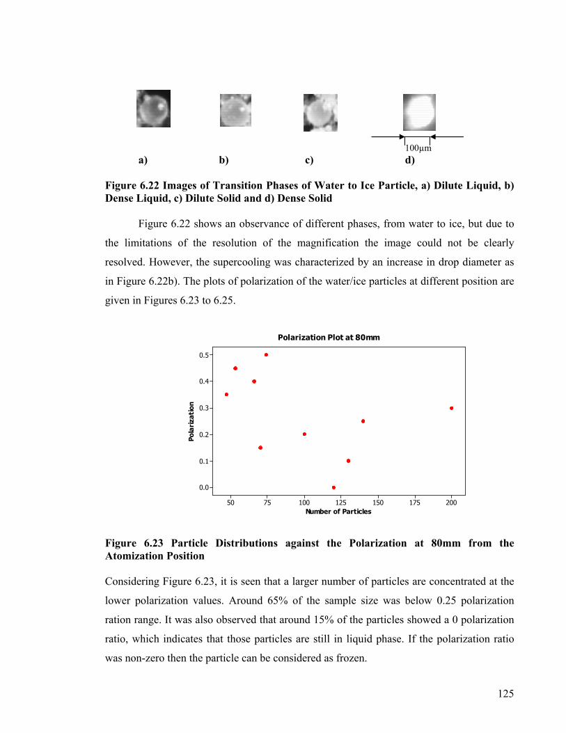
a) b) Figure 6.22 Images of Transition PhasesDense Liquid, c) Dilute Solid and d) Dens

Figure 6.22 shows an observance o

the limitations of the resolution of the m

resolved. However, the supercooling was c

in Figure 6.22b). The plots of polarization o

given in Figures 6.23 to 6.25.

Pola

riza

tion

7550

0.5

0.4

0.3

0.2

0.1

0.0

Polar Figure 6.23 Particle Distributions agaAtomization Position Considering Figure 6.23, it is seen that a la

lower polarization values. Around 65% o

ration range. It was also observed that arou

ratio, which indicates that those particles a

was non-zero then the particle can be consid

c)

of Water to Ice Parte Solid

f different phases, from

agnification the ima

haracterized by an inc

f the water/ice particl

Number of Particles150125100

ization Plot at 80mm

inst the Polarizatio

rger number of particl

f the sample size was

nd 15% of the particle

re still in liquid phase

ered as frozen.

100µm d)

icle, a) Dilute Liquid, b)

water to ice, but due to

ge could not be clearly

rease in drop diameter as

es at different position are

200175

n at 80mm from the

es are concentrated at the

below 0.25 polarization

s showed a 0 polarization

. If the polarization ratio

125

Number of Particles

Pola

riza

tion

200150100500

0.6

0.5

0.4

0.3

0.2

0.1

0.0

Polarization Plot at 200mm

Figure 6.24 Particle Distributions against the Polarization at 200mm from the Atomization Position Figure 6.25 Exchanger

In the

increased, bu

polarization r

Further, in F

particles are a

2%.

Number of Particles

Pola

riza

tion

160140120100806040200

0.6

0.5

0.4

0.3

0.2

0.1

0.0

Polarization Plot at 750mm

Particle Distributions against the Polarization at the Outlet of the Heat

Figure 6.24, the number of particles between the range of 0.25 and 0.6

t still 30% was seen below 0.25 polarization ratio. The presence of null

atio was also observed to be 7% and therefore tend to decrease with distance.

igure 6.25 the observation at the outlet revealed that more than 70% of the

bove 0.25 polarization ratio and the null polarization ratio decreased to 1 to

126

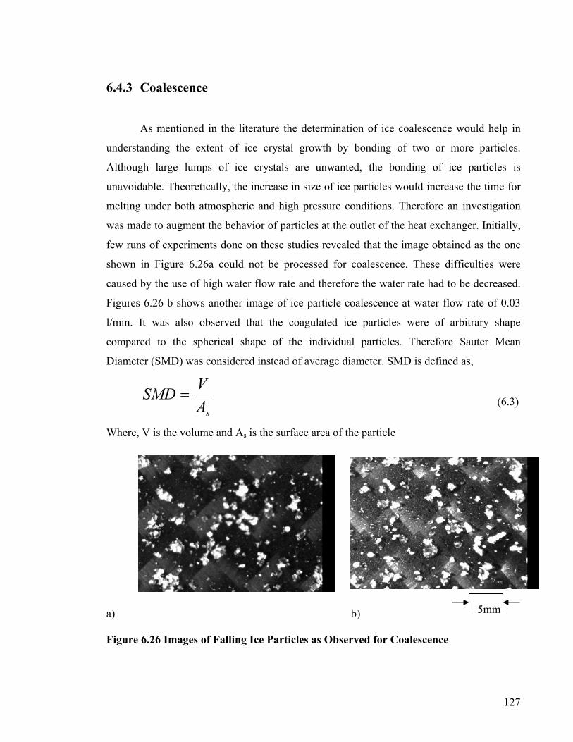
6.4.3 Coalescence

As mentioned in the literature the determination of ice coalescence would help in

understanding the extent of ice crystal growth by bonding of two or more particles.

Although large lumps of ice crystals are unwanted, the bonding of ice particles is

unavoidable. Theoretically, the increase in size of ice particles would increase the time for

melting under both atmospheric and high pressure conditions. Therefore an investigation

was made to augment the behavior of particles at the outlet of the heat exchanger. Initially,

few runs of experiments done on these studies revealed that the image obtained as the one

shown in Figure 6.26a could not be processed for coalescence. These difficulties were

caused by the use of high water flow rate and therefore the water rate had to be decreased.

Figures 6.26 b shows another image of ice particle coalescence at water flow rate of 0.03

l/min. It was also observed that the coagulated ice particles were of arbitrary shape

compared to the spherical shape of the individual particles. Therefore Sauter Mean

Diameter (SMD) was considered instead of average diameter. SMD is defined as,

sAVSMD = (6.3)

Where, V is the volume and As is the surface area of the particle

a) b) 5mm Figure 6.26 Images of Falling Ice Particles as Observed for Coalescence

127

The parameters considered for the experiments are given in Table 6.15 and the plot

shown in Figure 6.27. The technique used to measure the SMD was adopted from the one

used for measuring mean diameter as discussed in Section 6.4.1.

Table 6.15 Parameters Considered for Measuring Coagulated Particle Diameter


Ice Particle Temperature, C

Coag

ulat

ed D

iam

eter

, mic

rom

eter

0-10-20-30-40-50-60-70

500

400

300

200

12010080

VariableInitial Ice Diameter, 120µmInitial Ice Diameter, 100µmInitial Ice Diameter, 80µm

Plot of Coagulated Diameter Figure 6.27 Plot of Coagulated Particles as a Function of Ice Particle Temperature

The variation of coagulated ice particles diameter was measured as a function of its

temperature. It was analyzed by leaving out the separate particles. It was observed that the

SMD increases steeply to 450µm when the temperature drops to -40°C and drops to 250µm

once the ice particles drop to -50°C. Further decrease in ice particle temperature does not

seem to affect the SMD. However, in general, the particle SMD has increased considerably

128

from its initial size. At -40°C, the particle SMD increased 3 to 4 times from its initial value

but decreased to a value of 2 to 2.5 on further reduction in ice particle temperature.

6.5 Measurement of Hardness

A qualitative analysis of ice hardness as a measure of temperature was conducted in

order to find out the reliability of ice particles. It was stated that, when the temperature of

the ice was lowered to -32°C the hardness would be equivalent to that of steel [40]. From

the literature [104] an effort was made to establish the measurement of the hardness in

terms of Brinell or Rockwell hardness. However, practically it was not feasible to find the

hardness of the ice particles of few hundred microns in diameter. Instead, 40mm ice cubes

at different temperatures were used to find their hardness using the Brinell hardness

method. The experiments were carried out using the parameters in the Table 6.16.

Table 6.16 Parameters for Brinell Hardness Test for Ice.

Load applied 100 kN

Indenter Diameter

10 mm

Time period allowed 5 sec

The experiments were carried out by lowering the ice cube temperature using

controlled flow of liquid nitrogen over it. Thermocouples of K-type were used to measure

the dynamic temperature of the ice and any temperature difference was compensated by

adjusting the flow of liquid nitrogen. The application of the load was initially varied and a

100kN was selected as a practical limit. Application of loads beyond this range resulted in

initiation of crack on the surface of the ice cube. Another constraint in using this

measurement technique was the time limitation. Higher the time period of the application of

the load, faster the melting rate at the indenter section. Controlling of the temperature at

that section was demanding with temperatures fluctuating, therefore a time limit of 5

seconds was used. The measurement was made with a temperature interval of 10°C. The

schematic diagram of the load application is shown in Figure 6.28.

129

Figure 6.28 Schematic

The hardness was calcu

BHN

where, F is the load ap

The Figure 6.29 shows

--70

Figure 6.29 Brinell H

From the plot,

decreases. However, th

of the Load Application for Brinell Hardness for Ice

lated from the formula

130

(6.4) )(2

22iDDDD

F

−−•= π

plied, D is the indenter diameter and Di is the indentation diameter

the variation of ice hardness in terms of Brinell hardness.

Ice Temperature, °C

Brin

ell H

ardn

ess,

HB

0-10-20-30-40-5060

160

140

120

100

80

60

40

20

Plot of Brinell Hardness

ardness as a Function of Ice Temperature

it is seen that the hardness increases as the temperature of the ice

e increase of hardness was found to reach a stable state after which

131

there was little or no variation. These BHN’s were then converted to Moh’s number for

qualitative comparison. It was found that, when converted to Moh’s hardness the values

were between 1.5 and 3, which could be comparable to the gypsum and calcite in the non-

metallic table.

6.6 Summary

To this end, the feasible experiments carried out within a range of practical

parameters by using available measuring techniques were discussed. The temperature

measurements suggest that very low temperature ice particles could be formed under

controlled environment with the use of optimal parameters. The visualization techniques

alluded quantitative measurements of the ice particle diameter (separate and coagulated)

and to an extent the observance of different phase of water/ice particles. The physical test

of the ice cubes suggests the possibility of using the ice particle entrainment into the high-

pressure Ice Jet nozzle.

Though the results were obtained experimentally, emphasis is also given to perceive

numerical simulation in the Chapter 7. These were done to extend the observed

experimental results to form computational analysis and to give a perspective insight into

the various experimentally unobserved phenomena of temperature distribution, particle

movement, drag forces and the mass fraction distributions.

132

Chapter 7

Numerical Modeling of Ice Particle Formation and Ice Jet Process

7.1 Introduction

The use of numerical simulations was to predict and gain an understanding of

the aspects of heat transfer phenomena computationally. For these studies a

Computational Fluid Dynamic (CFD) package, CFX was used. Extensive study of the

ice particle formation process was done by computation, with further emphasis given on

the study of behavior of ice particles inside the ice jet nozzle. Inside the heat exchanger,

temperature distributions at different planes, particle trajectories of the ice particles,

volume fractions of cryogenic nitrogen, ice particles and air, together with Velocity

Vectors of all phases were predicted with the governing equations detailed in Chapter 5.

After obtaining the results from the numerical analyses, the solutions were then

compared with the available experimental results. The extent of validation is also

discussed in this chapter. Later, in this chapter, the numerical results and discussions of

the ice jet process are given with a view to argue the feasibility of its usability.

7.2 Structure of CFX

CFX-5 is a general-purpose Computational Fluid Dynamics (CFD) code,

combining an advanced solver with powerful pre and post-processing capabilities. At

the initial stages of the simulation, CFX-4.4 was used, but owing to the limitations in

features of Inter-phase heat and mass transfer and restricted support of phase change

problems, an updated version CFX-5.6 was later used.

CFX-5.6 consists of five software modules which are linked by the flow of information

required to perform a CFD analysis. Figure 7.1 shows the structure of CFX-5.6.

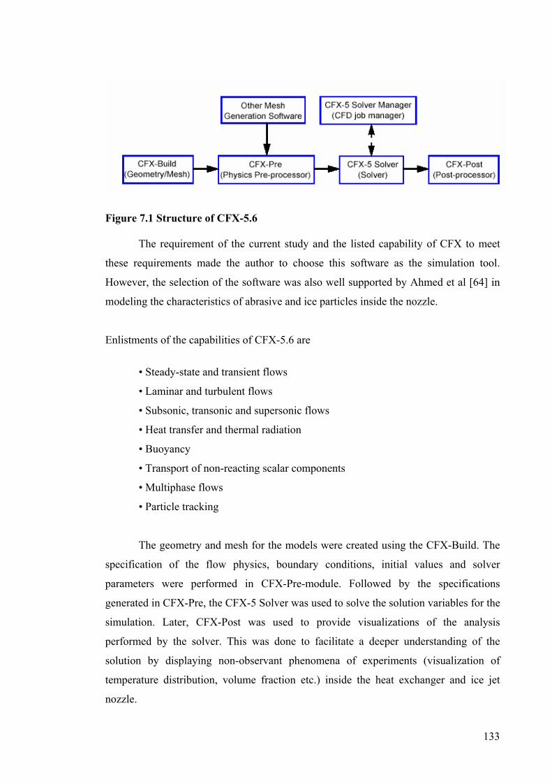
Figure 7.1 Structure of CFX-5.6

The requirement of the current study and the listed capability of CFX to meet

these requirements made the author to choose this software as the simulation tool.

However, the selection of the software was also well supported by Ahmed et al [64] in

modeling the characteristics of abrasive and ice particles inside the nozzle.

Enlistments of the capabilities of CFX-5.6 are

• Steady-state and transient flows

• Laminar and turbulent flows

• Subsonic, transonic and supersonic flows

• Heat transfer and thermal radiation

• Buoyancy

• Transport of non-reacting scalar components

• Multiphase flows

• Particle tracking

The geometry and mesh for the models were created using the CFX-Build. The

specification of the flow physics, boundary conditions, initial values and solver

parameters were performed in CFX-Pre-module. Followed by the specifications

generated in CFX-Pre, the CFX-5 Solver was used to solve the solution variables for the

simulation. Later, CFX-Post was used to provide visualizations of the analysis

performed by the solver. This was done to facilitate a deeper understanding of the

solution by displaying non-observant phenomena of experiments (visualization of

temperature distribution, volume fraction etc.) inside the heat exchanger and ice jet

nozzle.

133

7.3 Boundary Conditions

The equations relating to fluid flow can be closed (numerically) by the

specification of conditions on the external boundaries of a domain. It is the boundary

conditions that produce different solutions for a given geometry and set of physical

models. Hence, boundary conditions determine largely the characteristics of the solution

obtained. Therefore, it was important to set boundary conditions that accurately reflect

the real situation to obtain accurate results.

Solid Boundary

Fluid-Solid Interface

Fluid Boundary

Figure 7.2 Illustration of Fluid an

y

Air

d Solid Boundarie

Inlet Boun

s in He

Outlet Boundary
Cryogenic nitrogen Boundary
Water Inlet Boundar

dary

at Exchanger

134

In the heat exchanger shown in Figure 7.2, three inlets and one outlet were used.

The velocity components were specified by cylindrical coordinate with r, θ and z and

the flow rates were specified for all the inlets. To obtain the convergence, the total flow

rate of the inlet was assumed to be equal to that of the outlet. The boundary conditions

are given in Table 7.1.

Table 7.1 Boundary Conditions at Inlet and Outlet

Boundary Conditions Inlet boundaries

Inlet1 Cryogenic Nitrogen

Temperature -100°C and -120° C Volume fraction 1.0 i.e., 100% cryogenic nitrogen flowing through inlet1 Flow rate 0.5, 1.0 and 1.5 l/min

Inlet2 Water

Temperature 5°C, 10°C, 15°C, 20°C Volume fraction 1.0 i.e., 100% water flowing through inlet2 Flow rate 0.03, 0.1 and 0.2 l/min

Inlet3 Air Temperature 10°C Volume fraction 1.0 i.e., 100% air flowing through inlet3 Flow rate 0.25, 0.5 and 0.75 l/min Outlet boundary

Air + Ice particles + Nitrogen Type pressure boundary Pressure 1 bar

7.4 Grid Independence Test

Convergence of the simulation is defined for an algorithm, where appropriate

solution closes to the theoretical correct solution with minimum number of integration

step. However, the total convergence solutions of the simulations depend on the

geometry, its coordinate system, meshes and other factors such as boundary conditions,

choosing appropriate model and inlet conditions. Minimum number of integration steps

varies with the above conditions, but, occasionally convergence solutions may be

unrealistic, making grid independence test necessary.

135

Before starting a CFD calculation, it is necessary to perform a grid independence

test for all geometries and models. This was done to determine the minimum number of

grids needed to generate a solution for the model. At the initial stage of the simulation a

coarse grid was used and then it was increased until the deviation of the results became

negligible. The geometry was split into four blocks as shown in Figure 7.3. Figure 7.4

shows the grids of the heat exchanger in three-dimensional planes. A fixed grid

approach was adopted owing to the advantage of using this against moving grid in

tracking the solid-liquid interface as per the discussions in the literature [75, 77 and 78].

It was also selected due to the advantage of using unique set of equations and boundary

conditions for the entire domain. As the geometry was created with cylindrical

coordinate system, the number of grid points in the r and θ directions were kept constant

throughout the heat exchanger (i.e. for all four blocks) and the convergence criteria was

obtained with the use of smaller grid size. These are given in Table 7.2.

Table 7.2 Number of Grids on Each Axis for the Heat Exchanger

Block Number r θ Z

1 15 30 20

2 15 30 100

3 15 30 20

4 15 30 20

Block 1

Block 2

Block 3

Block 4

136
Figure 7.3 Representation of Heat Exchanger Blocks

Figure 7.4 Three-Dimensional Grids of Heat Exchanger

The physical property of water/ice and cryogenic nitrogen such as density, heat

capacity, and thermal conductivity were assumed to change with temperature.

Imbedding functions to estimate the changing properties adds complexity to the models,

but increases the accuracy and better fits with the experiments. To account for the

changing properties model, polynomial equations were fitted to the data [85, 105]. The

physical properties and equations used for the model predictions for a given temperature

are shown in Table 7.3.

A forward difference time discretization was used to solve the transient droplet

temperature, that is, for each time step, the droplet volume was recalculated to

compensate for the volume change due to mass transfer. The internal heat transfer of the

droplet was solved after taking into account the ice volume change.

137

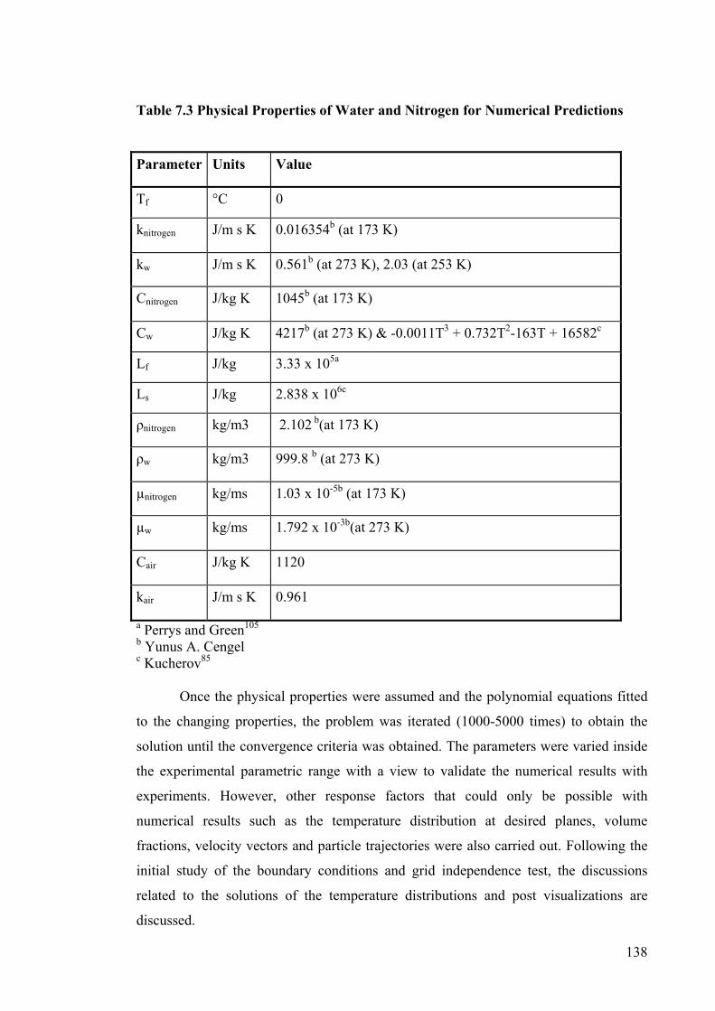
138

Table 7.3 Physical Properties of Water and Nitrogen for Numerical Predictions

Parameter Units Value

Tf °C 0

knitrogen J/m s K 0.016354b (at 173 K)

kw J/m s K 0.561b (at 273 K), 2.03 (at 253 K)

Cnitrogen J/kg K 1045b (at 173 K)

Cw J/kg K 4217b (at 273 K) & -0.0011T3 + 0.732T2-163T + 16582c

Lf J/kg 3.33 x 105a

Ls J/kg 2.838 x 106c

ρnitrogen kg/m3 2.102 b(at 173 K)

ρw kg/m3 999.8 b (at 273 K)

µnitrogen kg/ms 1.03 x 10-5b (at 173 K)

µw kg/ms 1.792 x 10-3b(at 273 K)

Cair J/kg K 1120

kair J/m s K 0.961

a Perrys and Green105

b Yunus A. Cengel c Kucherov85

Once the physical properties were assumed and the polynomial equations fitted

to the changing properties, the problem was iterated (1000-5000 times) to obtain the

solution until the convergence criteria was obtained. The parameters were varied inside

the experimental parametric range with a view to validate the numerical results with

experiments. However, other response factors that could only be possible with

numerical results such as the temperature distribution at desired planes, volume

fractions, velocity vectors and particle trajectories were also carried out. Following the

initial study of the boundary conditions and grid independence test, the discussions

related to the solutions of the temperature distributions and post visualizations are

discussed.

139

7.5 Temperature Distribution Study 7.5.1 Visualization at Different Planes

Pertaining to the limited experimental observation of the temperature

distribution along the vertical axis of the heat exchanger, effort was taken to extend the

study on temperature distribution of X-Y plane along the Z-axis. The initial parameters

set forth in the boundary conditions for the real parameters were iterated using the

Solver and visualized by Post processor. However, for the sake of understanding the

visualization results were discussed first and followed by the quantitative analysis of

temperature variation through different plots. The range of parameters selected to obtain

temperature variation is given in Table 7.4.

Table 7.4 Parameters Considered for Ice Particle Temperature along the Heat Exchanger

Cryogenic Nitrogen Temperature °C -100, -120 Cryogenic Nitrogen Flow Rate l/min 0.5, 1, 1.5 Inlet Water Temperature °C 5, 10, 15 Droplet diameter µm 80, 100, 120 Water Flow Rate l/min 0.2 (constant) Inlet Angle degrees 30 (constant) Air temperature °C 10 (constant) Air flow rate l/min 1.5 (constant)

In predicting the temperature distribution on the X-Y plane, three points on the Z-axis

were of interest.

1. the plane where cryogenic nitrogen and water droplets first contact

2. the plane where all water droplet temperatures drop below 0°C

3. at the outlet of the heat exchanger

This analysis was done to project the effect of inlet cryogenic flow rate, its

temperature, inlet water temperature and droplet diameter on different points and to put

forward an argument to show the extent of under surface or over surface design of the

heat exchanger. Figures 7.5 to 7.8 show the temperature distribution of water droplets

for nitrogen flow rate of 0.5 and 1.5 l/min, temperature of -100°C and -120°C and inlet

water temperature of 5°C and 15°C. It should be noted that the water droplets were

treated as dispersed phase with nitrogen and air taken as continuous phase. To make the

discussions easier the selection of parameters was classified into four different inlet

conditions. The inlet conditions for the study are given in Table 7.5.

Table 7.5 Classification of Parameters

Water

Temperature,

°C

Cryogenic Nitrogen

Temperature, °C

Cryogenic Nitrogen

Flow rate, l/min

Inlet Condition 1 5 -100 0.5




Fig

Con

part

disc

ure 7.5 Temperature Distribution of Water Droplets in XY plane for Inlet

dition 1

140

Because the water droplets were considered as dispersed phase rather than

icles, the temperature distribution is represented by continuous shade instead of

ontinuous patches. It was also seen that the selection of the model based on three

dimensions rather than symmetric plane helped in observance of the entire XY plane.

The selection of latter would only have shown one half of the result.

Figure 7.6 Temperature Distribution of Water Droplets in XY plane for Inlet

Condition 2

Comparing Figures 7.5 and 7.6 for the effect of nitrogen flow rate, no obvious

difference could be interpreted. With a change in 1 l/min there was no significant

change observed at the point of initial contact between both fluids except for 1°C

difference.

Fi

Co

gure 7.7 Temperature Distribution of Water Droplets in XY plane for Inlet

ndition 3

141

The effect of water temperature on the initial contact region does not give any

quantitative difference in terms of temperature distribution. It was calculated that there

was a 3°C difference for both cases i.e. at inlet water temperature of 5°C and 15°C.

With the Figure 7.8, the high temperature region seems to be more predominant than the

low temperature regions.

Fi

Co

tem

l/m

tem

alt

the

the

dis

po

inl

ca

ax

gure 7.8 Temperature Distribution of Water Droplets in XY plane for Inlet

ndition 4

Figures 7.5 to 7.8 were comparable for the difference in the inlet nitrogen

perature made on the initial contact region. With the nitrogen flow rate kept at 1.5

in the temperature distribution was predicted to vary only a little. Overall the

perature difference seemed to be same. Changing the parameters at the inlet does not

er the temperature at the point of contact. All results pertain to be the same and

refore it was hypothesized that there was no instantaneous transfer of heat between

se fluids. This could also be due to the fact that both water droplets and nitrogen

place with time in the downward Z direction and there was not enough time at this

int for an instantaneous heat transfer to occur. Therefore, the analysis of the effect of

et conditions at the point where the temperature of all droplets fall below 0°C was

rried out. Figures 7.9 to 7.12 show the temperature distribution in XY plane in the Z-

is at different inlet conditions.

142

FC

FC

igure 7.9 Temperature Distribution of Water Droplets in XY plane for Inlet ondition 1


143


FC


144

145

Again, as per the visualization for the plane of contact, the plane at which the

temperature of water droplets fall below 0°C revealed some facts to be understood only

by discussions. For the inlet condition 1, the water droplets turn to ice particles at a

distance of 450mm from the water droplet inlet. This was supported by the fact that the

heat transfer between the fluids was low and thus resulted in a longer time period and

distance. The temperature distribution was in the range of 0°C to -7°C with most of the

area occupied with mean temperatures. The increase of nitrogen flow rate in Figure 7.10

showed a decrease in the distance and time the water droplets drop below 0°C. The

increase of flow rate by three times from 0.5 l/min to 1.5 l/min resulted in a reduction of

the length of ice particle formation by 250mm. It was also characterized by a decrease

in overall temperature on the plane with the minimum temperature dropping to -15°C.

Further, the temperature of water was increased and the temperature distribution

observed as shown in Figure 7.11. With the increase in inlet water temperature the

distance of water droplets freezing increased. Quantitative result show that the distance

of ice particle formation plane increased by 100mm with the inlet temperature increased

by 10°C. On the other hand, the mean temperature only increased by 2°C. This

observation shows that the temperature at this plane has less dependency on the inlet

water temperature within the given range.

With the effect of nitrogen flow rate and inlet water temperature observed, the

inlet nitrogen temperature was decreased to -120°C as in Figure 7.12. However, to

emphasize, the variation of nitrogen temperature from room temperature was time

dependent and was taken from the observation discussed in Section 6.2.1 of Chapter 6.

The temperature alone was decreased keeping other parameters constant. This

constituted a decrease in the distance the water drops fall below 0°C. The results show

that the drop of temperature below 0°C occurred at a distance of less than 100mm from

the inlet position. The mean temperature was, however, the same as that of the Figure

7.10 and largely occupied by low temperature regions. These results direct an argument

to evaluate the parameters from the most influential to the least influential or otherwise

expressed as the predictors. Nevertheless, this needs further study and continuance

prediction of the ice particle temperature along the Z-axis and to the outlet.

The most important of all was the prediction of ice particle temperature along

the outlet of the heat exchanger. This was done to validate the results obtained from the

experiments. Figures 7.13 to 7.16 show the temperature distribution of ice particles at

the outlet of the heat exchanger. The name of the legend was renamed as “Ice” instead

of “water droplet temperature” to avoid possible confusion from the misnomer. From

Figure 7.13, it can be seen that the ice particles reach a temperature of -30°C with the

entire plane pertaining to a near constant temperature. Another observation made from

this prediction was the decrease in temperature with respect to distance. It was seen that

it took 450mm for the water droplets to drop below 0°C, and another 300mm to drop to

-30°C. At this point of discussion it is not clear whether this was the effect of under

surfaced heat exchanger. Therefore, few more predictions were needed to arrive at a

conclusion to predict this effect.

FC F

t

r


igures 7.14, 7.15 and 7.16 show the temperature distribution with increased nitrogen

emperature, increased water temperature and decreased nitrogen temperature

espectively.

146



147


As discussed earlier, the nitrogen flow rate was increased keeping the other

parameters constant and the results are shown in Figure 7.14. By doing this, the

temperature at the outlet further dropped sharply by 25°C. This was a phenomenal

decrease in temperature and was accelerated by a three time increase in flow rate. The

average temperature was found to be -57°C with temperature near the walls fluctuating

by ±1°C. In other terms, for a distance of 550mm (from the point at which the

temperature of water droplets falls below 0°C), the temperature drop was -57°C.

Further, by increasing the inlet water temperature by 10°C, the ice particle

temperature increased by 7°C. The overall temperature seemed to decrease to -50°C

with a travel distance of 450mm from the point on the Z-axis where the temperature

dropped to 0°C. Decrease of nitrogen temperature further to -120°C resulted in an outlet

mean temperature of -63°C. However, the travel distance from the point of 0°C

increased to 650mm. These results interpret a qualitative solution to the argument of

whether it was under surfaced, but outlet temperature of the cryogenic nitrogen was also

necessary to extend this argument. The heat exchanger was seemingly under surfaced

and these discussions are later expanded in Section 7.6.2 to give quantitative answers.

148

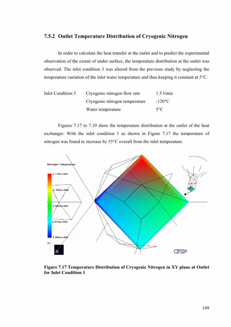
7.5.2 Outlet Temperature Distribution of Cryogenic Nitrogen

In order to calculate the heat transfer at the outlet and to predict the experimental

observation of the extent of under surface, the temperature distribution at the outlet was

observed. The inlet condition 3 was altered from the previous study by neglecting the

temperature variation of the inlet water temperature and thus keeping it constant at 5°C.

Inlet Condition 3 Cryogenic nitrogen flow rate 1.5 l/min

Cryogenic nitrogen temperature -120°C

Water temperature 5°C

Figures 7.17 to 7.19 show the temperature distribution at the outlet of the heat

exchanger. With the inlet condition 1 as shown in Figure 7.17 the temperature of

nitrogen was found to increase by 55°C overall from the inlet temperature.

Ff

igure 7.17 Temperature Distribution of Cryogenic Nitrogen in XY plane at Outlet or Inlet Condition 1

149

Ff

Ff

c



150

By increasing the flow rate of nitrogen and keeping the other parameters

onstant, it was noted that the outlet temperature difference decreased. It was also seen

that, between the sidewalls, there was a 5°C difference and only the mean temperature

was taken for the reference. The temperature reduction of 20°C directed to a hypothesis

that, if the length of the heat exchanger were increased there would have been more

transfer of energy between the ice particles, air and nitrogen. However, in the current

study the increase in length was not extrapolated. Continuing with the simulation the

nitrogen temperature was decreased to -120°C and thereby the results show a 28°C

difference between the inlet and final temperatures.

7.5.3 Air Temperature at the Outlet

The temperature distribution of air is shown for an understanding of the

temperature difference between the inlet and outlet conditions. Though it was thought

that the visualization of air temperature was not conditional, the observation at the outlet

gave an indication of the energy gained by air when mixed with cryogenic nitrogen.

With the inlet temperature of air set at 10°C, the temperature distribution is shown in

Figure 7.20.

FC

igure 7.20 Temperature Distribution of Air in XY plane at Outlet for Inlet ondition 1

151

7.6 Temperature Plots 7.6.1 Ice Particle Distribution

The discussion of the temperature distribution was further quantified by the

prediction of temperature along the sidewalls. The inlet conditions were set as per the

earlier discussions and the temperature variation plotted as shown in Figures 7.21 and

7.22. The observation revealed that the variation was linear and the temperature

difference for the inlet condition 1 was lower compared to the temperature difference of

the inlet condition 3. Temperatures reached -20°C with inlet condition 1 and decreased

to -50°C as the flow rate of nitrogen was increased and to -60°C as the nitrogen

temperature was decreased.

152

Distance, mm

Tem

pera

ture

, C

8007006005004003002001000

0

-10

-20

-30

-40

-50

-60

0

0

VariableInlet Condition 1Inlet Condition 2Inlet Condition 3

Water/Ice Temperature Along Side Walls

Figure 7.21 Temperature of Ice Particles along the Side walls

Distance, mm

Tem

pera

ture

, C

8007006005004003002001000

0

-10

-20

-30

-40

-50

-60

-70

0

0

0


Water/Ice Temperature Along Vertical Axis Figure 7.22 Temperature Variation of Ice Particles along the Vertical axis Excluding the Side walls

Pertaining to the follow-up of the discussions, the plot of temperature along the

vertical axis was done to find out the difference in the wall temperature to the rest of the

heat exchanger, and is shown in Figure 7.22. It was studied that, there was no difference

in the trend lines of the temperature variation, but in fact, the temperature on an average

was 10°C lesser in the area other than the sidewalls. This was due to the flow of air

along the sidewalls both in upward and downward direction, which resulted in an

increase in ice particle temperature at the walls.

7.6.2 Temperature Variation Study

Cryogenic nitrogen and ice particle temperature variations along the z-axis were

studied and are shown in Figures 7.23 to 7.25. This was done for the inlet conditions

specified earlier and was plotted for an interval of 100mm from the inlet position. It was

seen that, the ice particle temperature gradually decreased on the other hand, nitrogen

temperature gradually increased. Although it was experimentally proven that the

designed heat exchanger was under surfaced, validation of simulation with experiments

was highly desired. Though in theory it was the case, the important fact was in finding

out whether these two curves merge at some point before reaching the outlet position. If

that was the case then the heat exchanger surface would be over surfaced else it could

be concluded that the heat exchanger was under surfaced.

Temperature Variation, Inlet Condition 1

Figure 7.23Condition 1

Distance, mm

Tem

pera

ture

, C

8007006005004003002001000

0

-20

-40

-60

-80

-100

0

0

VariableIce ParticlesCrogenic Nitrogen

Temperature Variation of Ice Particles and Nitrogen for Inlet

153

Figure Conditi


Figure Conditi

I

particles

Figure 7

increase

the pred

tempera

experim

7.24 Temperature Variation of Ice Particles and Nitrogen for Inlet on 2

Distance, mm

Tem

pera

ture

, C

8007006005004003002001000

0

-20

-40

-60

-80

-100

0

0

VariableIce ParticlesCryogenic Nitrogen

7on

t

.2

d

ic

tu

en

154

Distance, mm

Tem

pera

ture

, C

8007006005004003002001000

0

-20

-40

-60

-80

-100

-120

0

0VariableIce ParticlesCryogenic Nitrogen


.25 Temperature Variation of Ice Particles and Nitrogen for Inlet 3

was predicted that, as the nitrogen flow rate was increased to 1.5 l/min the ice

temperature decreased to -60°C. This was similar to the case observed in

5, but at a lower temperature. The decrease of nitrogen temperature further

the difference in the outlet temperature. From these facts it was concluded that

tions agree with that of the observed phenomena of the experiments. Thus the

re curves in the simulations at various length intervals extrapolated the

tal results and gave an insight into the temperature difference at those points.

7.6.3 Air Temperature

Another study pertaining to predict the temperature behavior of air along the

upward direction and downward direction was set forth. Figure 7.26 shows the variation

in both directions and along the walls of the heat exchanger. For convenience, a local

coordinate system was taken thereby considering the inlet position as 0mm and the

upward direction to be on the negative scale of the axis. As both air and nitrogen were

taken as continuous phase the heat transfer from nitrogen to air was performed without

any limitation. The heat transfer from ice particles (dispersed phase) to air was also

possible with the way the boundary condition were initialized. However, the ice

particles in general was not affected by the direct heat transfer and rather alluded by air

(i.e. air temperature affects nitrogen and that in turn affects ice particle temperature),

except at ice particles impact on the side walls.

Figure 7.26

With

predicted t

temperature

temperature

nitrogen pr

high. With t

5°C. Furthe

Distance, mm

Tem

pera

ture

, C

3002001000-100-200

10.0

7.5

5.0

2.5

0.0

-2.5

-5.0

0

0


Air Temperature Variation

Air Temperature Variation along the Side walls

all inlet conditions taken for the comparison of air temperature, it was

hat the air temperature decreases in both directions. However, the

on the upward direction seemed to decrease to a larger extent than the

on the downward direction. This was due to the lower temperature of

esent at the upper half of the heat exchanger. Therefore heat transfer was

he inlet temperature of air at 10°C, the lowest temperature observed was at -

r assessments of the model with the experiments are given in Section 7.10.

155

7.7 Volume Fraction

Theoretically, it was assumed that the volume/mass flow of all the inlets was

equal to that of the outlets. In this current study there were three inlets with the

assumption that each inlet was assumed to compose of 100% of the phase. Thereby,

only one phase was allowed to pass into each inlet and this was the case in experiments.

The outlet was assumed to compose a mixture of all these phases in proportion.

Therefore it was necessary to predict the proportions at different length intervals and to

interpret the results thus showing the behavior of these continuous and dispersed phases

inside the heat exchanger. However, the visualizations are first shown with the plot of

different length intervals.

Figure 7.27 shows the volume fraction of ice particles for the inlet condition1.

This is a proportionate volume fraction and was seen that the higher and lower range of

the volume are concentrated on the one section of the plane and leaving the average

volume fraction to concentrate on the other side. This improper volume fraction was an

effect of the focus direction of the flow rate of nitrogen. This could however be rectified

if both fluids run together, but practical limitations would prevent this by happening.

FH

igure 7.27 Volume Fraction of Ice Particles on the XY plane at the Outlet of the eat Exchanger

156

In the Figure 7.28, similar effect was observed with the volume fraction

concentrating on the one section of the plane and leaving an improper distribution. The

effect of volume fraction on equal intervals along the Z axis had to be predicted to

understand the volume expansion or depression at that point.

Fiof

an

7.3

ind

to

co

ex

rea

de

int

air

ne

gure 7.28 Volume Fraction of Cryogenic Nitrogen on the XY plane at the Outlet the Heat Exchanger

To pursue the preceding discussions, plots of volume fractions of air, nitrogen

d ice particles were predicted for 0.5, 1.0 and 1.5 l/min as shown in Figures 7.29 to

1. It should be taken into account at any plane along the Z-axis that the sum of all the

ividual volume fractions must be equal to one.

From Figure 7.29, it was observed that the volume fraction of nitrogen increases

a distance of 200mm and decreases rapidly to 0.45 at 400mm, thereafter, it prevails

nstant until the outlet. This effect was caused by the introduction of air into the heat

changer at a distance of 500mm from the inlet position. The upward movement of air

ched a distance of 200mm and thus caused the volume fraction of nitrogen to

crease. Whereas, the volume fraction of ice particles seemed to decrease until the

roduction of air and then increased until it reached the outlet. The volume fraction of

decreased rapidly from 0.4 at the inlet to 0.1 in the upward direction, but remained a

ar constant in the downward direction.

157

Figure 7.29 Volume Fraction of Different Phases at Nitrogen Flow rate of 0.5 l/min Figure 7.30 Volume Fraction of Different Phases at Nitrogen Flow rate of 1.0 l/min

Distance, mm

Vol

ume

Frac

tion

8007006005004003002001000

0.9

0.8

0.7

0.6

0.5

0.4

0.3

0.2

0.1

0.0

VariableIce ParticlesAirCryogenic Nitrogen

Volume Fraction, Nitrogen Flow Rate-1.0 l/min

Distance, mm

Vol

ume

Frac

tion

8007006005004003002001000

0.8

0.7

0.6

0.5

0.4

0.3

0.2

0.1

0.0


Average Volume Fraction, Nitrogen Flow Rate-0.5 l/min

Figure

158

Distance, mm

Vol

ume

Frac

tion

8007006005004003002001000

0.9

0.8

0.7

0.6

0.5

0.4

0.3

0.2

0.1

0.0


Volume Fraction, Nitrogen Flow Rate-1.5 l/min

7.31 Volume Fraction of Different Phases at Nitrogen Flow rate of 1.5 l/min

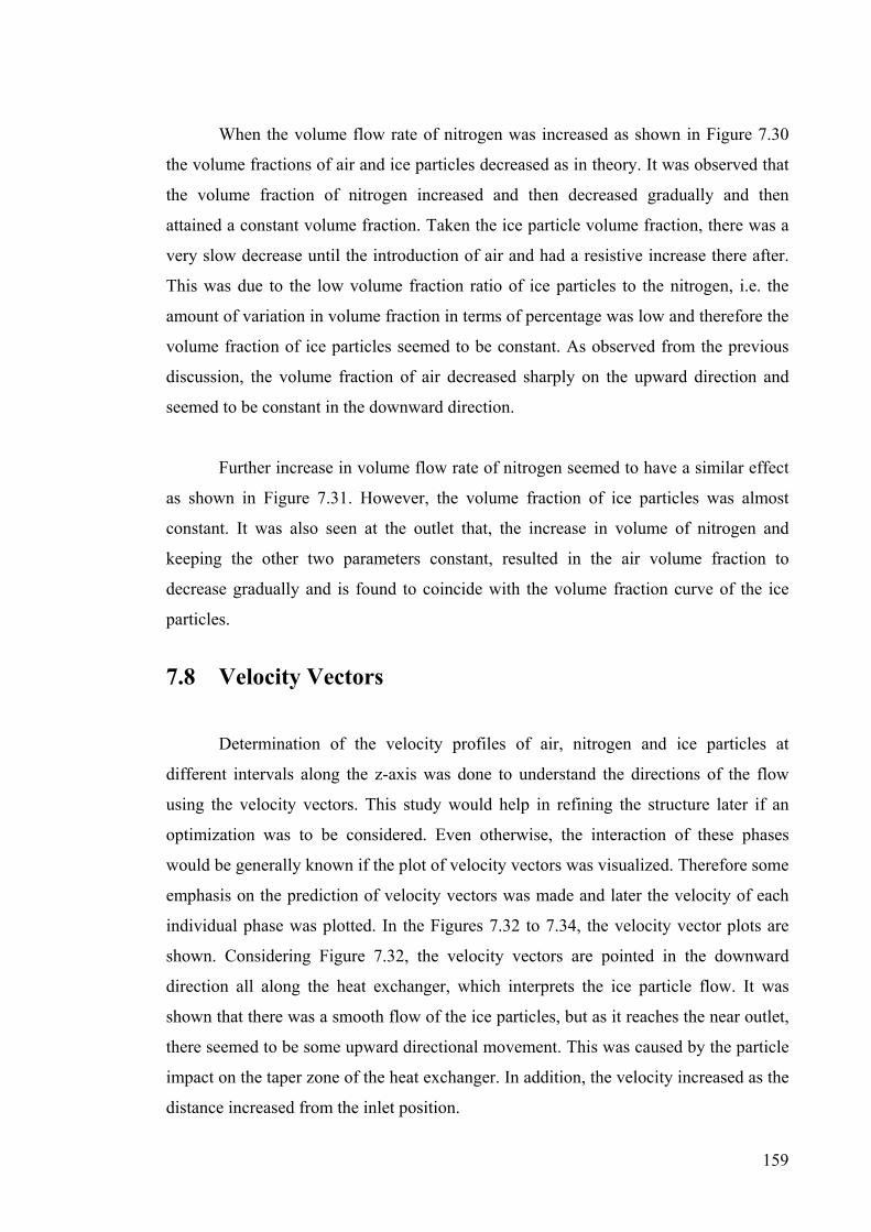
159

When the volume flow rate of nitrogen was increased as shown in Figure 7.30

the volume fractions of air and ice particles decreased as in theory. It was observed that

the volume fraction of nitrogen increased and then decreased gradually and then

attained a constant volume fraction. Taken the ice particle volume fraction, there was a

very slow decrease until the introduction of air and had a resistive increase there after.

This was due to the low volume fraction ratio of ice particles to the nitrogen, i.e. the

amount of variation in volume fraction in terms of percentage was low and therefore the

volume fraction of ice particles seemed to be constant. As observed from the previous

discussion, the volume fraction of air decreased sharply on the upward direction and

seemed to be constant in the downward direction.

Further increase in volume flow rate of nitrogen seemed to have a similar effect

as shown in Figure 7.31. However, the volume fraction of ice particles was almost

constant. It was also seen at the outlet that, the increase in volume of nitrogen and

keeping the other two parameters constant, resulted in the air volume fraction to

decrease gradually and is found to coincide with the volume fraction curve of the ice

particles.

7.8 Velocity Vectors

Determination of the velocity profiles of air, nitrogen and ice particles at

different intervals along the z-axis was done to understand the directions of the flow

using the velocity vectors. This study would help in refining the structure later if an

optimization was to be considered. Even otherwise, the interaction of these phases

would be generally known if the plot of velocity vectors was visualized. Therefore some

emphasis on the prediction of velocity vectors was made and later the velocity of each

individual phase was plotted. In the Figures 7.32 to 7.34, the velocity vector plots are

shown. Considering Figure 7.32, the velocity vectors are pointed in the downward

direction all along the heat exchanger, which interprets the ice particle flow. It was

shown that there was a smooth flow of the ice particles, but as it reaches the near outlet,

there seemed to be some upward directional movement. This was caused by the particle

impact on the taper zone of the heat exchanger. In addition, the velocity increased as the

distance increased from the inlet position.

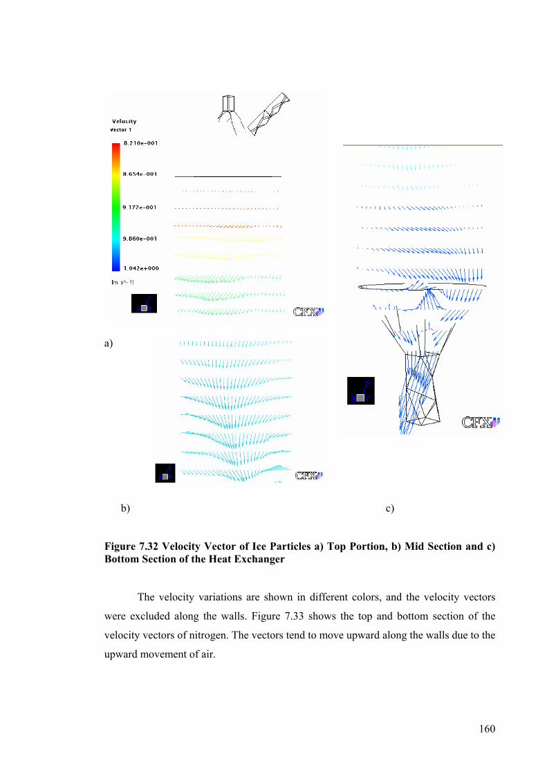
a)

b)

Figure 7.32 Velocity Vector of Ice Particles a) ToBottom Section of the Heat Exchanger

The velocity variations are shown in differe

were excluded along the walls. Figure 7.33 shows

velocity vectors of nitrogen. The vectors tend to mov

upward movement of air.

160

c)

p Portion, b) Mid Section and c)

nt colors, and the velocity vectors

the top and bottom section of the

e upward along the walls due to the

a)

b) Figure 7.33 Velocity Vecthe Heat Exchanger In the Figure 7.34, the ai

upwards and downwards o

of velocities at different in

tor of Nitrogen a) Top Portion and b) Bottom Section of

r movement represented in two-dimension was seen to rise

n the walls. Following up with the vector plots are the plots

tervals and are shown in Figures 7.35 to 7.37.

161

Figure 7.34 V

Vel

ocit

y, m

/s

--

Figure 7.35 V

Vertical axis

As sh

with increase

due to gravity

the outlet. T

elocity Vector of Air at the Mid Section of the Heat Exchanger

Distance, mm8007006005004003002001000

1.20

1.00

0.80

0.60

0.40

0.20

0.000.050.10

0

0

VariableVelocity-WallVelocity-Vertical Axis

Velocity-Water/Ice Particles

elocity Variations of Ice Particles along the Sidewalls and along the

own in Figure 7.35 the velocity of water/ice particles gradually increase

in vertical distance. This was due to the fact that particles are accelerated

from an initial value of 0.8 m/s and reaches a maximum value of 1 m/s at

he inter-phase drag between the particles and the nitrogen resisted the 162

velocity increase and therefore was gradual. Another observation on the effect of

velocity on the side walls was also plotted. The velocity until the distance of 200mm

was zero and from 200mm there appears a velocity plot of 0.4 m/s. This was due to the

fact that, water/ice particles impact on the side walls at this distance and therefore

generate a velocity plot. This velocity decreases to zero and then its direction was

reversed thereby a negative velocity was seen at a distance of 400 to 500mm. This was

due to the upward flow of air causing the ice particles to travel in the upward direction.

Further, from the distance of 500mm, the velocity increased to 0.2m/s and remained

constant until the outlet.

The nitrogen velocity (function of flow rate) was also determined and the results

are shown in Figure 7.36. Contrary to the ice particle velocity, nitrogen velocity

decreases as the distance from the inlet increases. The inlet velocity of the nitrogen was

kept at 0.6 m/sec and found to decrease to 0.1 m/sec at the outlet. This was because the

cryogenic gas expands and due to the momentum transfer to the ice particles and air, the

velocity decrease occurred. Another reason for the decrease in velocity was due to the

increase in temperature of the nitrogen as it flows downwards and thus loosing density.

Figure 7.

the Verti

Distance, mm

Vel

ocit

y, m

/s

8007006005004003002001000

0.6

0.5

0.4

0.3

0.2

0.1

0.0

-0.1

-0.2

0

0

VariableVelocity-WallVelocity-Vertical Axis

Velocity-Cryogenic Nitrogen

36 Velocity Variation of Cryogenic Nitrogen on the Sidewalls and along

cal axis

163

The nitrogen velocity on the wall is found to decrease and then found to flow in

the opposite direction. However, the representation of the velocity to distance in this

particular case was limited by a higher time intervals selected. As observed from the

results of ice particle velocity profile, the velocity of nitrogen on the side walls past the

inlet point of air in the downward direction was found to increase. This velocity was in

par with the velocity of the air, therefore it can be said that the flow of air had a high

influence on the acceleration of nitrogen.

The Figure 7.37 shows the velocity profile of air inside the heat exchanger. The

observation of this velocity profile was found to be more complicated but when plotted

it was well understood. The position of the air inlet was kept as 0mm reference and the

negative direction indicates the upward movement of air and the positive direction

indicates the downward discharge of air. In studying the upward direction along the

wall, the air velocity was found to decrease with respect to distance and at 200mm from

the position, the air velocity reaches almost 0 m/s and started flowing in the opposite

direction. However, the velocity of air in the negative direction was on the vertical axis

and not on the wall. The downward direction of the air movement was straight forward

with the air velocity increasing along the walls until the outlet. The downward flow of

air in the vertical axis was also found to accelerate after 100mm from the air inlet

position. This effect was caused by the stray air mixed with the flowing nitrogen and

due to the decrease in air temperature and the cold air on the vertical axis other than the

wall flows down. However, the volume fraction of the air flowing through the center

axis was negligible and was not considered to affect the ice particle temperature.

Figure 7.

Distance, mm

Vel

ocit

y, m

/s

3002001000-100-200

0.3

0.2

0.1

0.0

-0.1

0

0

VariableVelocity-WallVelocity- Vertical Axis

Velocity-Air

37 Velocity Variation of air along the sidewalls and along the vertical axis

164

7.9 Particle Trajectory of Water

The visualization of the particle track was done by using Lagrangian method due

to the limited visualization of the Eulerian method. So, the general particle track could

only be shown with the particles assumed as ice particles and without any phase change.

However, the important factor in predicting the particle track was its Reynolds number

and the formulae used are discussed in Section 5.4.1 of Chapter 5. The diameter of the

particles assumed was 120µm (for abrasive particle size) with 50 particles set at the

inlet plane of the atomization point. Figure 7.38 shows the particles behavior inside the

heat exchanger and is seen that some particles impact the wall on the lower half of the

surface.

Figure 7.38 Partic

Having giv

particles was predi

by using Eulerian m

two fluids as contin

particles on side wa

le Track of Ice Particles Inside the Heat Exchanger

en the visualization plots, analysis of the volume fraction of ice

cted by varying the inlet nitrogen flow rate. However, this was done

ethod by considering ice particles as dispersed phase and the other

uous phase. Figure 7.39 shows the impact of volume fractions of ice

lls for inlet nitrogen flow rates of 0.5, 1.0 and 1.5 l/min.

165

FiDi

im

pa

l/m

fro

Fu

pa

at

of

dis

in

the

sh

be

flo

cir

Distance, mm

Vol

ume

Frac

tion

0.24

0.18

0.12

0.06

0.00

700-

750

600-

700

500-

600

400-

500

300-

400

200-

300

100-

200

0-10

0

0.3

0.2

0.1

0.0

700-

750

600-

700

500-

600

400-

500

300-

400

200-

300

100-

200

0-10

0

0.3

0.2

0.1

0.0

Vfrac Ice, Set1 Vfrac Ice, Set2

Vfrac ice, Set3

Volume Fraction of Ice Particles Impact on Side Walls

Flow Rate 1.5 l/min

Flow Rate 1.0 l/min Flow Rate 0.5 l/min

gure 7.39 Volume Fraction of Ice Particles Impact on Side walls at Increasing stance

When the cryogenic nitrogen was set at 0.5 l/min the ice particles were found to

pact the surface at the distances of 600 to 750mm. There was negligible fraction of

rticles impacting the distances from 0 to 600mm. With an increase in flow rate to 1.0

in the ice particles impact on the surface increased with the impact distance starting

m 400mm. This caused an increase in the volume fractions of the particle impact.

rther increase of cryogenic flow rate to 1.5 l/min contributed to an increase in the

rticle impact not only in the distance range of 400 to 750mm but also a steep increase

a distance of 100 to 200mm. This was caused by the directional projection of the flow

cryogenic nitrogen. Higher the flow rate, higher the velocity of the nitrogen as

cussed earlier in this chapter. Therefore increase in flow rate constituted an increase

the particles being projected onto the walls at a distance of 100 to 200mm.

Consideration of streamlines (for continuous phase) was also given to determine

extent of cryogenic nitrogen and air behavior inside the heat exchanger. Figure 7.40

ows the flow rate at and beyond 1.5 l/min. It can be seen that the increase of flow rate

yond 1.5 l/min constitutes flow to project onto the surface and then worsens as the

w rate was increased. Figure 7.41 shows the streamline flow of air. This shows a

cular motion along the walls and a twisted circular motion along the vertical axis.

166

Fi2.5

Fi

a) b) c) gure 7.40 Streamlines of Cryogenic Nitrogen at a) 1.5 l/min, b) 2.0 l/min and c) l/min

gure 7.41 Streamlines of

167

Airflow along the Wall and along the Vertical axis.

7.10 Model Assessment

The validation of the temperature measurements was done with the solution

obtained for various inlet nitrogen temperatures. Though previous discussions were

pertained to the study of temperature variations at different planes on the heat

exchanger, a time dependent temperature variation was not discussed. In this Section,

however, the numerical temperature variations were plotted along with experimental

results. Figures 7.42 to 7.44 shows the plots for different inlet nitrogen flow rates,

temperatures and water temperatures.

The cryogenic nitrogen temperature was reduced systematically as per the

experimental measurements done in Section 6.2 of Chapter 6. In doing this, the

properties of the ice particles were recalculated from Table 7.3. Therefore, to make the

numerical simulations agree better with the experiments the properties were calculated

at every degree fall in temperature. To make the plots clearly distinguishable, a time

interval of 20 seconds was taken. These predictions were done for the same time period

as that of experimental results.

Figure 7Variation

Time, Sec

Ice

Part

icle

Tem

pera

ture

, C

200180160140120100806040201

0

-10

-20

-30

-40

-50

-60

-70

00Variable

Numerical, IC1Numerical, IC2

Experimental IC1Experimental, IC2

Function of Inlet Cryogenic Nitrogen Temperature

.42 Experimental and Simulated Results of Ice Particle Temperature s for Varying Cryogenic Nitrogen Temperature

168

Time, Sec

Ice

Part

icle

Tem

pera

ture

, C

200180160140120100806040201

0

-10

-20

-30

-40

-50

-60

-70

0

Variable

Experimental, IC3Numerical, IC1Numerical, IC2Numerical, IC3

Experimental, IC1Experimental, IC2

Function of Cryogenic Nitrogen Flow Rate

Figure 7.43 Experimental and Simulated Results of Ice Particle Temperature Variations for Different Nitrogen Flow Rate

Time, Sec

Ice

Part

icle

Tem

pera

ture

, C

200180160140120100806040201

20

10

0

-10

-20

-30

-40

-50

-60

0

Variable

Experimental, IC3Numerical, IC1Numerical IC2Numerical, IC3

Experimental, IC1Experimental, IC2

Function of Water Temperature Figure 7.44 Experimental and Simulated Results of Ice Particle Temperature Variations for Different Inlet Water Temperature

It was observed in Figures 7.42 to 7.44 that the experimental and numerical

predictions agree each other largely, with both the temperature curves almost super

imposing on each other. Though this was the case, in almost all plots the numerical

predicted temperature was below the experimental temperature. This study was

extended by varying the flow rate and inlet water temperature. Although the trend lines

seemed to be similar, some experimental temperatures on the time scale seemed to drop

below the numerically predicted value. This could have been due to the experimental

uncertainty at that point of time. These results formulate reliable predictions in terms of

169

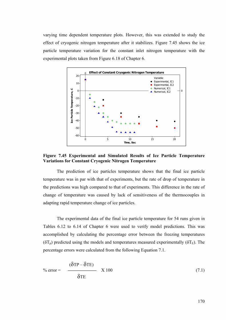
varying time dependent temperature plots. However, this was extended to study the

effect of cryogenic nitrogen temperature after it stabilizes. Figure 7.45 shows the ice

particle temperature variation for the constant inlet nitrogen temperature with the

experimental plots taken from Figure 6.18 of Chapter 6.

0 Effect of Constant Cryogenic Nitrogen Temperature

Figure 7.45 Variations fo

The p

temperature w

the prediction

change of tem

adapting rapid

The e

Tables 6.12

accomplished

(δTp) predicte

percentage er

% error =

Time, Sec

Ice

Part

icle

Tem

pera

ture

, C

20151050

20

10

0

-10

-20

-30

-40

-50

-60

0

VariableExperimental, IC1Experimental, IC2Numerical, IC1Numerical, IC2

Experimental and Simulated Results of Ice Particle Temperature r Constant Cryogenic Nitrogen Temperature

rediction of ice particles temperature shows that the final ice particle

as in par with that of experiments, but the rate of drop of temperature in

s was high compared to that of experiments. This difference in the rate of

perature was caused by lack of sensitiveness of the thermocouples in

temperature change of ice particles.

xperimental data of the final ice particle temperature for 54 runs given in

to 6.14 of Chapter 6 were used to verify model predictions. This was

by calculating the percentage error between the freezing temperatures

d using the models and temperatures measured experimentally (δTE). The

rors were calculated from the following Equation 7.1.

(δTP – δTE) X 100 (7.1) δTE

170

Figure 7.46 Frequency Diagram of the Percentage Error between Ice Particle Temperature Difference between Experiments and the Model

FiguExp

mod

This

expe

expe

The

re 7.4erimen

T-D

iff-E

xper

imen

t

7

6

5

4

3

The

el havin

gave

riments

riments

refore i

7 Best fit of the Ice Particle Temperature Difference between the ts and the Model

T-Diff-Model7060504030

0

0

0

0

0

S 3.33903R-Sq 93.4%R-Sq(adj) 93.3%

171

frequency graph in Figure 7.46 shows the temperature variable property

g error within ± 10% with the maximum frequency that occurs at +1.5%.

an indication of the level of agreement between the model and the

. This was further extended to study the best fit of the prediction to the

as shown in Figure 7.47. This shows the R-squared value of 93.4%.

t can be said that the model has a good agreement in terms of determining

the final ice particle temperature at the outlet of the heat exchanger. The reason for this

good agreement of the results predicted by variable properties models with the

experimental results was due to the significant variation of specific heat capacity taken

into account by the model.

The visualization experiments carried out to determine the polarization of ice

particles was qualitatively compared to the numerical results. As discussed in Chapter 5

there are four stages in transforming water droplets to ice particles. Therefore as per the

visualization experiments the simulation was done at 80mm, 200mm and at the outlet to

determine the phase distribution. Figures 7.48 to 7.50 show the pie chart of the phase

distribution as a function of temperature given in Table 7.6.

Table 7.6 Interpretation of Phase in terms of Temperature

Dilute liquid 5°C and above

Dense liquid 0°C to -5°C

Dilute solid -10°C to 0°C

Dense solid -10°C and below

Different Phase of Water/Ice at 80mm

Dilute Liquid

Dense Liquid

Dilute Solid

Dense Solid

28%

35%

25%

12%

Figure 7.48 Phase Distribution at 80mm from the Inlet Position for Inlet

Condition3

172

Different Phase of Water/Ice at 200mm

Dilute Liquid

Figure 7.49 Pha

Condition 3

Figure 7.50 Phase

As per the

dense liquid occup

distance from the

25% of the volume

with 93% and som

compared with the

increasing polariza

The numeri

experimental resul

temperature within

these simulations

25%

Dense Liquid

Dilute Solid

Dense Solid

se Distrib

Differe

Distributi

prediction

ying a vol

inlet increa

respective

e 7% of d

experimen

tion with in

cal model t

ts. In these

the experi

was done

42%

ution at 200mm fro

nt Phase of Water/Ice at

on at the Outlet for In

, all four phases exist

ume of 35% followed

sed dilute solid and d

ly by proportion. How

ilute solid was predic

tal analysis revealed

creasing distance.

o this extent was conc

analyses it was show

mental range was well

to provide an idea of

20%

13%

m the Inlet position for Inlet

Outlet

Dilute Liquid
93%
Dense Liquid
7% Dilute Solid
Dense Solid

let Condition 3

ed at the distance of 80mm, with

by dilute liquid with 28%. As the

ense solid contributed to 42% and

ever, at the outlet only dense solid

ted to be present. This fact when

a closer qualitative agreement with

entrated into the intrapolation of the

n that the prediction of ice particle

agreed. However, extrapolation of

predictor factors in improving or

173

optimizing the experimental design. But the current study was limited in providing only

a brief prediction of the extrapolated results.

7.11 Extrapolation of Numerical Model

The extrapolation of the numerical results was preferable because of the good

agreement of the results to the experiments. The cryogenic nitrogen temperature could

be kept at liquid state (below -197°C), thereby predicting the consequences of its effect

on the ice particle temperature. The droplet diameter could be increased owing to its

least influence of its inlet values to the outlet temperature. Both cryogenic nitrogen and

water droplets could be allowed to transfer heat from the inlet point of water droplets.

Therefore, a study was made to foresee the effects at perfect conditions as per the

theory. Figure 7.51 shows the ice particle temperature at the outlet with varying inlet

conditions.

0

Figu

Exp

The

the

temp

prac

Distance, mm

Ice

Tem

pera

ture

, C

8007006005004003002001000

0

-25

-50

-75

-100

0

VariableNitrogen Temp, -140CNitrogen Temp, -160CNitrogen Temp, -200C

re 7.51 Extrapolated Ice Particle Temperature for Cryogenic Nitrogen below

erimental values

plot predicts the temperature of ice particles below the experimental values set by

current study. At liquid nitrogen temperature i.e. below -197°C, ice particle

erature was predicted to be -95°C. However, consideration should be given in

tice to obtain these conditions.

174

With the brief discussion of the extrapolated results, the focus was drifted

towards the formation of numerical analysis of the ice transportation system and the ice

jet nozzle. As discussed earlier, these analyses were made to study the survival of ice

particles in the due course of mixing with high-pressure, high-velocity fluid inside the

nozzle. Though some literature was found into the numerical model of ice jet (Section

2.4.6 of Chapter 2), analysis was carried out with inter-phase heat and momentum

transfer with particular attention given to heat transfer among all fluids (i.e. heat transfer

between air-ice, air-water and water-ice). In the succeeding Section 7.12 the ice

transportation to the nozzle is analyzed and discussed.

7.12 Ice Slurry Transportation System Ice particles produced from the heat exchanger were transported to the water/air

jet nozzle by the use of transportation system. In designing this system, accountability

was taken in providing a lengthier tube for flexible movement of the nozzle. Therefore,

a length of 1.5m with a diameter of 10mm corresponding to the measurements of the

available abrasive tube was taken for this current study. The transportation system

comprises of one inlet and one outlet boundaries. The velocity components were

specified by cylindrical coordinate with r, θ and z. The outlet condition of the heat

exchanger was taken as the inlet conditions for the transportation system. As an

assumption the total inlet mass flow rate was kept equal to the outlet. This was however

important to obtain a convergence. The inlet/outlet conditions are given in Table 7.7 (a)

and (b).

Table 7.7 (a) Boundary Conditions for Inlet of Ice Slurry Transfer System

Inlet Condition 1 Inlet Condition 2 Inlet Condition

3

Ice temperature, °C -30 -50 -70

Air temperature, °C 7.5 2.5 -2.5

Nitrogen temperature, °C -45 -65 -80

Volume fraction (ice) 0.2 0.15 0.1

Volume fraction (nitrogen) 0.4 0.6 0.7

Volume fraction (air ) 0.4 0.25 0.2

175

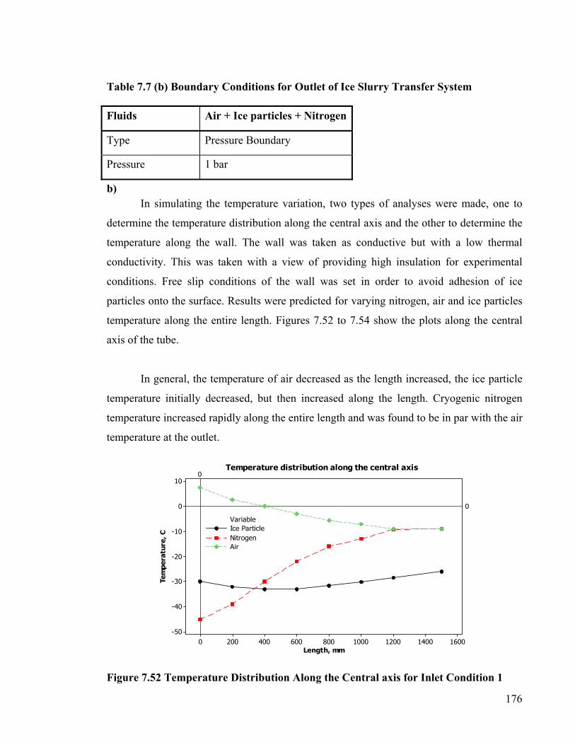
Table 7.7 (b) Boundary Conditions for Outlet of Ice Slurry Transfer System

In simulating the temperature variation, two types of analyses were made, one to

determine the temperature distribution along the central axis and the other to determine the

temperature along the wall. The wall was taken as conductive but with a low thermal

conductivity. This was taken with a view of providing high insulation for experimental

conditions. Free slip conditions of the wall was set in order to avoid adhesion of ice

particles onto the surface. Results were predicted for varying nitrogen, air and ice particles

temperature along the entire length. Figures 7.52 to 7.54 show the plots along the central

axis of the tube.

In general, the temperature of air decreased as the length increased, the ice particle

temperature initially decreased, but then increased along the length. Cryogenic nitrogen

temperature increased rapidly along the entire length and was found to be in par with the air

temperature at the outlet.

Fluids Air + Ice particles + Nitrogen

Type Pressure Boundary

Pressure 1 bar

b)

Length, mm

Tem

pera

ture

, C

16001400120010008006004002000

10

0

-10

-20

-30

-40

-50

0

0

Variable

Air

Ice ParticleNitrogen

Temperature distribution along the central axis


176

Length, mm

Tem

pera

ture

, C

16001400120010008006004002000

0

-10

-20

-30

-40

-50

-60

-70

0

0

Variable

Air



Figure 7.53 Temperature Distribution Along the Central axis for Inlet Condition 2 Figure 7.54 T

These

length. This

particle tempe

ice particle

equilibrium t

the heat exch

nitrogen temp

Length, mm

Tem

pera

ture

, C

16001400120010008006004002000

0

-10

-20

-30

-40

-50

-60

-70

-80

-90

0

0

Variable

Air



emperature Distribution Along the Central axis for Inlet Condition 3

representative graphs show the ice particles temperature increased along the

was due to the presence of the third fluid (air). The initial decrease in ice

rature was due to the fact that cryogenic nitrogen temperature was below the

temperature and equilibrium condition was not achieved yet. Once the

emperature has reached at 200 to 400mm length, the theoretical behavior of

ange would further freeze the ice particles with an increase in cryogenic

erature. However, due to the presence of air high inter-phase heat transfer

177

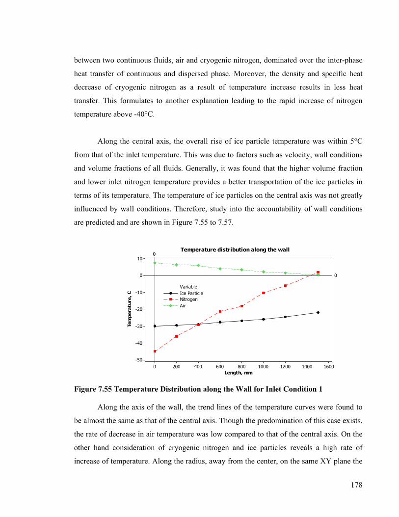
between two continuous fluids, air and cryogenic nitrogen, dominated over the inter-phase

heat transfer of continuous and dispersed phase. Moreover, the density and specific heat

decrease of cryogenic nitrogen as a result of temperature increase results in less heat

transfer. This formulates to another explanation leading to the rapid increase of nitrogen

temperature above -40°C.

Along the central axis, the overall rise of ice particle temperature was within 5°C

from that of the inlet temperature. This was due to factors such as velocity, wall conditions

and volume fractions of all fluids. Generally, it was found that the higher volume fraction

and lower inlet nitrogen temperature provides a better transportation of the ice particles in

terms of its temperature. The temperature of ice particles on the central axis was not greatly

influenced by wall conditions. Therefore, study into the accountability of wall conditions

are predicted and are shown in Figure 7.55 to 7.57.

Length, mm

Tem

pera

ture

, C

16001400120010008006004002000

10

0

-10

-20

-30

-40

-50

0

0

Variable

Air


Temperature distribution along the wall Figure 7.55 Temperature Distribution along the Wall for Inlet Condition 1

Along the axis of the wall, the trend lines of the temperature curves were found to

be almost the same as that of the central axis. Though the predomination of this case exists,

the rate of decrease in air temperature was low compared to that of the central axis. On the

other hand consideration of cryogenic nitrogen and ice particles reveals a high rate of

increase of temperature. Along the radius, away from the center, on the same XY plane the

178

temperature of the fluids increases and on approaching the wall it was found to be at its

maximum.

Figure 7.56 Figure 7.57

The

to the incre

temperature

the radius

conduction,

in practical

from gainin

Temperature Distribution along the Wall for Inlet Condition 2

Length, mm

Tem

pera

ture

, C

16001400120010008006004002000

0

-10

-20

-30

-40

-50

-60

-70

0

0

Variable

Air


Temperature distribution along the wall

T

se

as

r

of

t

tr

g
179
Length, mm

Tem

pera

ture

, C

16001400120010008006004002000

0

-10

-20

-30

-40

-50

-60

-70

-80

-90

0

0

Variable

Air


Temperature distriution along the wall

emperature Distribution along the Wall for Inlet Condition 3

facts were due to two reasons, one due to the wall temperature and other due

e in momentum transfer of these fluids to the wall. At the walls, the average

ise was around 5°C, which gives an indication of temperature drift towards

the wall. If the walls were kept at isothermal conditions with no heat

he temperature change along the radius would have been constant. However,

ansportation, any high insulation on the walls would not prevent the fluids

temperature towards the wall. The outlet ice temperature compared to the inlet

temperature gained an overall temperature of 10°C, but increased with increase in inlet

cryogenic nitrogen temperature. As air was also present the cryogenic nitrogen loses energy

and therefore attains a high temperature. At the outlet of the transportation tube, nitrogen

and air was found to have almost same temperature regardless of the inlet nitrogen

temperature. The air temperature decreased gradually and was almost linear with increase

in length. As discussed earlier this was due to the decrease in density and specific heat of

the source, nitrogen.

The temperature distribution at the outlet is shown in Figure 7.58. This is however

shown with the mean temperature. Along the wall and inwards, the temperature was -60°C,

from the center and outwards, the temperature was bound to be -55°C. Though, the ice

temperature increased by 10°C, considering the physics of ice at that temperature, there was

negligible physical property change. Therefore the feasibility of entrainment of ice into the

nozzle with the high pressure water/air was thought of worth investigating by numerical

analyses. These are discussed in Section 7.13.

Fith

gure 7.58 Mean Temperature Distribution of Ice Particles Around the Walls and at e Central axis on the XZ plane at the Outlet

180

181

7.13 Ice Jet

To this extent, the ice particle formation and ice transportation to the nozzle have

been discussed. The results are promising with controlled temperature ice formation. These

were done with laminar flow owing to a small Reynolds number. However, the entrainment

of ice particles with a high-pressure, high-velocity nozzle was simulated under turbulent

conditions, the equations of which are discussed in Section 5.4.6 of Chapter 5.

The design of the nozzle geometry was taken form the existing Abrasive Water Jet

nozzle used in Industrial Research Institute Swinburne (IRIS). The existing design had a

diameter of 1mm at the exit of the nozzle with a taper entrance diameter of 4mm. This

constituted a high concentration of ice particles at the exit with the use of air as the jet. In

order to compensate for that effect, the air pressure had to be increased. Though

numerically the increase of air pressure would predict the behavior, practically increasing

the air pressure beyond 0.75Mpa could result in increase vibrations and noise [40]. This

effect was however an assumption, therefore the nozzle was scaled two times to

compensate for this cause. The Figure 7.59a) shows the real Abrasive Water Jet (AWJ)

nozzle with two inlets, one for the high-pressure water and other for the abrasives. The

abrasives are mixed with water in a mixing chamber, but in the current study only a

simplified version of the nozzle was used without the mixing chamber as shown in Figure

7.59b). The overall length of the nozzle was kept at the same length (100mm) as that of the

conventional nozzle.

The emphasis was only given to study the survival of ice particles in the due course

of mixing with high-pressure water/air. Therefore only a simple design was orchestrated.

Only preliminary results were obtained and discussed to find out the existence of ice phase.

The analyses were done for water and air with different air and water pressure and the

results obtained are discussed. In doing so, the boundary conditions and grid independence

test are described in Sections 7.13.1 and 7.13.2.

a) b) Figure 7.59 a) Conventional Nozzle used for AWJ in IRIS, b) Modified Nozzle Created for Numerical Ice Jet 7.13.1 Boundary Conditions

The outlet parameters of the ice transportation system were kept as the inlet

parameters for one inlet of the ice jet, for the other inlet the pressure and temperature of the

high-pressure fluids were varied accordingly. The Table 7.8 shows the inlet boundary

conditions.

Table 7.8 Initial Conditions of Inlet1 and Inlet2 of Ice Jet Nozzle

Inlet 2 Inlet 1 Condition 1 Condition2

Nitrogen Secondary air

Ice Ice Air Water

Pressure (MPa)

0.1 0.1 0.1 0.1 0.5-1.0 100-200

Temperature, C

-10 -15 -60 -60 0-25 0-25

182

The Figure 7.60 shows the inlet and outlet of the nozzle with the entire domain.

Figure 7.60 Inlet and O

7.13.2 Grid Independ

As per the analy

eliminate the influence o

environment, the use of f

the grid independence te

for each block on the cy

forms the block1, the inl

zone at the outlet forms b

utlet Boundaries of the Nozzle

ence Test

sis, the grid independence test for the nozzle was necessary to

f grids on the convergence. In this case owing to the multi-phase

ixed grid approach was adopted. More discussions of the details of

st are given in Section 7.4. Three blocks were used and the grids

lindrical axis are given in Table 7.9. The main body of the nozzle

et 2 projected onto the main body constitutes block2 and the taper

lock3.

183

Table 7.9 Number of Grids on Each Axis for the Nozzle

Representation of the grids in a three dimensional axis is shown in Figure 7.61. The

concentration of the grids was increased along the taper zone at the exit of the nozzle.

Block Number r θ Z

1 12 12 40

2 12 12 15

3 12 12 20

Figur 7.13.

of ice

variou

was n

by Liu

diame

airflow

was m

e 7.61 Three-dimensional representations of grids for the nozzle

3 Air Ice Jet

The main aim of entraining air into the nozzle was to analyze temperature variation

particles along the length of the nozzle. Researches into the air ice jet were done on

s applications and are discussed in Chapter 2. However, the temperature distribution

ot discussed. The air pressure was varied based on the parameters used for cleaning

[40], but the mass flow rate of ice was set to 0.2 kg/min in this current study. The

ter of ice particles were kept at 200µm and the inlet air temperature varied. An

rate of 0.83 m3/min was set as per the experiments done by Liu [40]. Initially a plot

ade to study the effect of cold nitrogen and secondary air (air from inlet2) as shown 184

in Figure 7.62. It is seen that the ice particles entering at a distance of 25mm increases by

almost 20°C in temperature. The other fluids entering from inlet2 also increase in

temperature and was found to be in level with the high pressure air at the exit. The rise of

temperature of high-pressure air was gradual and does not account to high temperature loss.

10

0

Figure 7.62

In F

and seconda

Figure 7.62

momentum

effect supe

compared t

particles to

Length, mm

Tem

pera

ture

, C

100806040200

0

-10

-20

-30

-40

-50

-60

0

Variable

NitrogenSecondary Air

IceAir

Temperature variation along the length of the nozzle

igure 7.63, the same simulations were repeated without the addition of nitrogen

ry air. The temperature of ice was found to vary with length, but compared to

it was found to be almost the same with no quantitative change. Due to the

of the air flowing at high velocity the ice particles increase in temperature, this

rcedes the inter-phase heat transfer. Though the specific heat of air is less

o that of the ice, the inter-phase momentum transfer effect caused the ice

increase to 20°C with only 10°C decrease in air temperature.

185

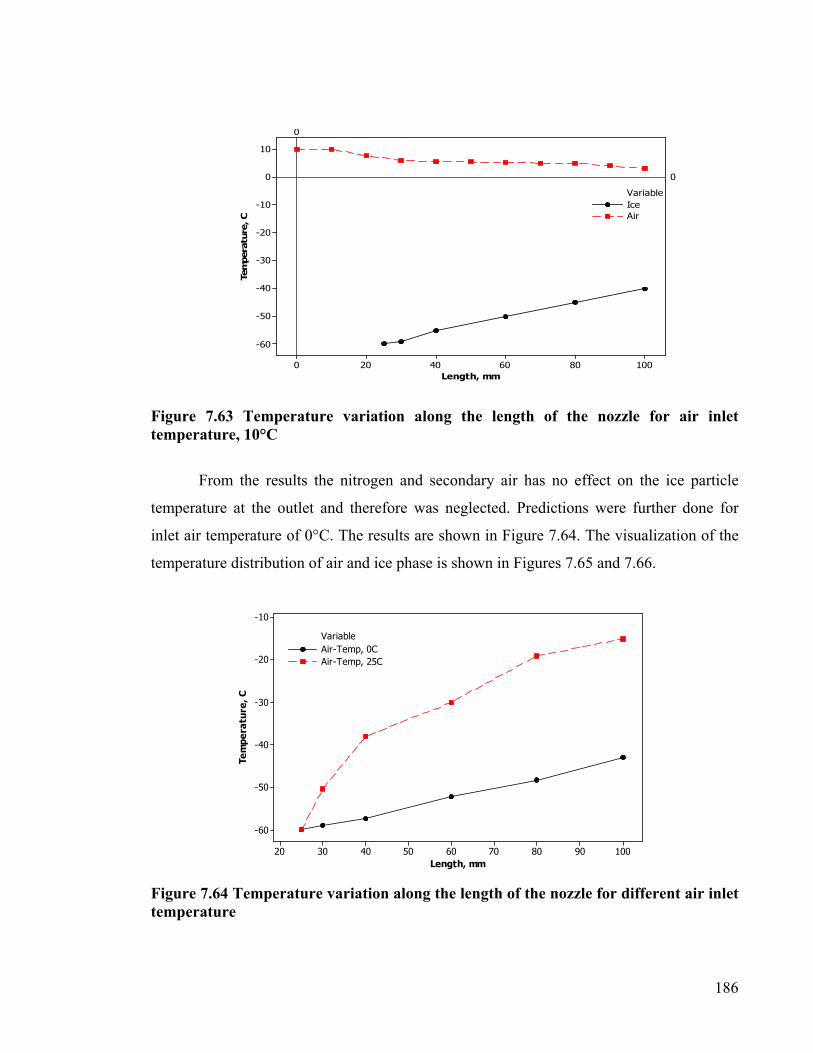
Length, mm

Tem

pera

ture

, C

100806040200

10

0

-10

-20

-30

-40

-50

-60

0

0

VariableIceAir

Figure 7.63 Temperature variation along the length of the nozzle for air inlet temperature, 10°C

From the results the nitrogen and secondary air has no effect on the ice particle

temperature at the outlet and therefore was neglected. Predictions were further done for

inlet air temperature of 0°C. The results are shown in Figure 7.64. The visualization of the

temperature distribution of air and ice phase is shown in Figures 7.65 and 7.66.

Figure 7.64temperatur

Length, mm

Tem

pera

ture

, C

1009080706050403020

-10

-20

-30

-40

-50

-60

VariableAir-Temp, 0CAir-Temp, 25C

Temperature variation along the length of the nozzle for different air inlet e

186

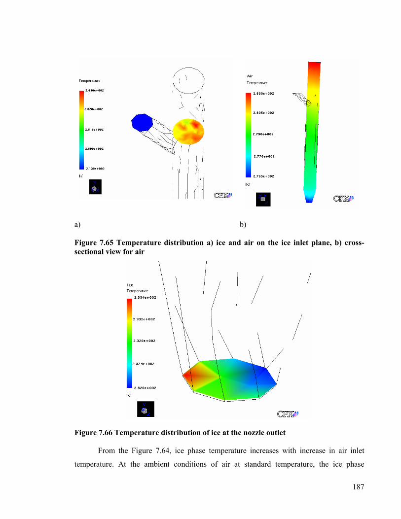
a) b Figure 7.65 Temperature distribution a) ice andsectional view for air Figure 7.66 Temperature distribution of ice at the

From the Figure 7.64, ice phase temperatu

temperature. At the ambient conditions of air at

)

air on the ice inlet plane, b) cross-

187

nozzle outlet

re increases with increase in air inlet

standard temperature, the ice phase

188

temperature increases by 45°C, thereby opening an argument into the reliability of its usage

in ice jet blasting. On the other hand as long the phase remains as ice, there exists a

feasibility of its usage in cleaning and blasting applications, but is subject to experiments.

The temperature distribution of air along the cross section shows a gradual decrease in air

temperature with temperature exiting at 2.5°C. The exit ice temperature shows no variation

in temperature distribution with the ice phase tending to -40°C on the entire plane. The

temperature distributions are given in Figure 7.65 and 7.66. The simulations were extended

to analyze the interaction of ice with the high-pressure water.

7.13.4 Water Ice Jet Simulations

These simulations were done by assuming the wall as non-conducting solid with the

buoyancy effect neglected. The existence of air as the third fluid was discussed in the

literature by Ahmed [64], however, in the current study the air was not accounted due to its

negligible flow. Initially, the pressure of the water was kept to 100MPa (i.e. third of the

actual pressure of AWJ) and the existence of ice phase test at the exit of the nozzle. Figures

7.67 and 7.68 show the temperature distribution of the ice phase along the length of the

nozzle for two inlet water temperature (10°C and 0°C). As the ice enters the mixing nozzle

there was a sudden increase in temperature and at a distance of 40mm the temperature starts

to rise linear until it exits. The sudden increase of temperature at the interface zone was due

to the impact of high velocity continuous flowing water on the near static ice velocity. This

effect was not observed when air was used instead of water and that was due to its low

velocity and pressure.

20

0 Figure 7.67 temperature Figure 7.68 temperature

The in

inter-phase h

rise in inlet w

the cause of t

other words

Length, mm

Tem

pera

ture

, C

100806040200

10

0

-10

-20

-30

-40

-50

-60

0

VariableIceWater

Temperature variation along the length of the nozzle for inlet water of 10°C

0

Length, mm

Tem

pera

ture

, C

100806040200

0

-10

-20

-30

-40

-50

-60

0

VariableIceWater

Temperature variation along the length of the nozzle for inlet water of 0°C

crease of temperature increases the outlet ice phase temperature due to the

eat transfer between the continuous phase and the dispersed phase. A 10°C

ater temperature only accounts to an ice phase temperature increase of 4°C,

his was due to the lack of proper inter-phase heat transfer at high velocities. In

the time duration was insufficient for a proper heat transfer to occur. The

189

temperature distributions of water and ice at the exit of the nozzle are shown in Figures

7.69 and 7.70.

Figu Figu

re 7.69 Temperature distribution of water at the nozzle exit on the XY plane

re
7.70 Temperature distribution of ice at the nozzle exit on the XY plane
190

191

It can be seen that the water temperature was almost constant at the exit with only a

1°C change. This was due to the assumption of non-conducting wall and a free slip on the

wall. This was the case with the ice with only 2°C difference between the central axis and

near the wall. This 2°C rise was triggered by the momentum transfer (not due to heat

transfer) of ice to the wall, thereby causing a difference in temperature. If the residence

time of ice increases there would be more time to allow a proper inter-phase heat transfer

causing the ice to gain more temperature. However, further decrease in residence time

could only be affected by an increase in pressure and this could cause high momentum

transfer and low heat transfer, therefore could result in negative effects.

7.13.5 Velocity Distribution

The velocity distribution for the entire domain with air and water as the accelerating

medium is shown in Figure 7.71. The velocity of the water was taken from the actual water

velocity of the AWJ but was scaled down to the pressure conditions used. For air, the

velocity was selected from Liu [40] and was kept at 10 m/s.

Figure 7.71a) shows a velocity drop at the entrance of the nozzle and then increases.

The increase of air velocity was short spanned and remained constant through out the main

body. In the taper zone near the exit the velocity increased to 215 m/s, this was due to the

contraction of the geometry of the nozzle at that exit. The observation of ice reveals the

increase of velocity from its static velocity and obtains enough acceleration to be in par

with the high velocity water. Figure 7.71b) shows a similar trend with increasing velocity

near the taper zone at the exit. The velocity was constant through out the main body at 10

m/s and there was no velocity drop found in the course of the entire domain. The velocity

of ice in this case behaves in the same way and accelerates from static velocity to the

velocity of the air jet. The reason for the water to experience a velocity drop might be due

to the high initial pressure exerted on the geometry causing a high pressure on the inner

surface of the walls. As the inner surface of the commercially available nozzle is made of

titanium, the walls of the model are assumed to have the property of titanium, the pressure

of the water was found to be distributed along the downward direction and therefore the

velocity increases after the initial drop.

Figure 7.71 Facial velocity of the nozzle domain on b) air-ice jet 7.13.6 Pressure Distribution

Analyzing the pressure distribution shown

decreasing until the interface and then increasing unt

at the interface. This was because the ice was kep

water pressure initially kept at 100MPa. In practical

creates a sudden pressure depression and thus ice par

effect of increase of pressure was studied over the

using water, the pressure was varied from 100 to 2

temperature with increasing pressure. At 100MPa t

30°C, increase of pressure to 200MPa changes the p

melts. These predictions reveal that by keeping a low

acceleration of high pressure water. Therefore, ic

potentially used for cutting brittle materials if not for

the YZ plane for a) water-ice jet

in Figure 7.72, it shows the pressure

il the exit. There exists a pressure drop

t at the atmospheric pressure and the

cases, the pressure drop at the interface

ticles are drawn inside the nozzle. The

temperature rise of the ice phase. In

00MPa. Figure 7.73 shows the rise of

he ice phase temperature increased by

hase of ice to water, therefore the ice

pressure, ice would survive the shear

e at very low temperatures could be

cleaning. 192

a) Figurinterf

Figurpressu

b)

e 7.72 Pressure distribution of ice-water domain a) presace b) entire domain

Length, mm

Tem

pera

ture

, C

9080706050403020

0

-10

-20

-30

-40

-50

-60

25

Va

20

1015

e 7.73 Temperature variation along the length of the nozzlre for water ice jet

sure drop at the

193

100

0

riable

0 Mpa

0 Mpa0 Mpa

e at different inlet

194

7.14 Conclusions

The study into the ice formation and ice jet has been discussed to the predictable

extent. It was found that the ice formation process was highly dependent on the cryogenic

nitrogen temperature and its flow rate. The variation of droplet diameter within the

experimental range had very little impact into the final ice particle temperature. The

predictions of the ice particles temperature were compared to the experimental temperature

and an assessment of the model was verified.

The overall error between the experiments and the model was also plotted to find

out a normal distribution. The entire ice formation process and the entrainment process was

catalyst by the advantage of reduction in solidification temperature of high-pressure water

from zero to -20°C. Though at high-pressure water temperature was varied from 0°C to

25°C, there exists a possibility of further reducing the inlet high-pressure water to -20°C

without freezing. Though the momentum transfer was high the ice particles did not melt at

the given inlet ice temperatures. However, the retention or the residence time was very

short, the probability of ice melting did not occur for pressures at and below 150MPa.

Recalling from the literature, at these outlet temperatures the ice has potential

implications in ice jet machining. It obeys the Hook’s law and is elastic between the

temperature range of -3°C and -40°C. Though the Ice Jet using high pressure water and air

are studied, accountability towards the actual experimentation of these predictions could be

the only way to verify the validations. However, this study was only limited to the

numerical modeling and consideration of the experimental work has been recommended to

further continuation.

Chapter 8

Conclusions and Recommendations 8.1 Introduction

This research work was undertaken to produce ice particles capable of surviving

high-pressure high-velocity water/air jet. In doing so, the work was divided into three parts.

The first part concentrated on the design and development of heat exchanger system and

investigations were carried out to determine the ice particle temperature, particle shape and

diameter, transition phase and hardness. The second part into the study was directed to

numerical analyses and predictions formulated to calculate the ice temperature distribution,

volume fraction, velocity vectors, particle trajectories and streamlines. The assessments of

these models were validated with the available experimental results. The overall results

showed that, ice particles could be produced at controlled and desired temperature with the

use of convective or direct heat transfer between two immiscible fluids.

The third part focused on temperature distribution of ice inside the transportation

system. It also analyzed the behavior of ice particles inside the ice jet nozzle. These

investigations were done by numerical analysis and results obtained indicate survival of ice

particles at the exit of nozzle up to a certain pressure. In the following sections, effort is

made to enlist the major contributions obtained from this current study. These are finally

followed up by recommendations for the further work.

8.2 Experimental Study of Temperature Measurements

The empirical study of the process parameters using One Factorial At a Time

(OFAT) reveals the ice particle temperature could be decreased to -60°C with the use of

very low temperature and high flow rate cryogenic nitrogen. However, the low ice

temperature was obtained within a certain optimum parametric settings. Though eight

195

factors were initially considered, some of the factors were experimentally kept constant to

avoid possible errors. The predictors were classified from the most significant to the least

significant and it was found that cryogenic nitrogen flow rate along with its temperature

were the most significant factors. The particle diameter was the least significant factor with

the final ice particle diameter not affected by inlet droplet diameter.

8.3 Visualization Study

The change of ice particle diameter with varying length of the heat exchanger was

carried out by visualization. Interpretation of the results reveals that there was a sudden

increase of ice particle diameter at a length of 80 to 200mm. Ice particle diameter was

found to decrease at the outlet, which lead to an observance of the occurrence of

supercooling at a distance of 80 to 200mm. The different phases of the transformation of

water droplets to ice particles were pictured for the diameter of around 100µm. Dilute

liquid, Dense liquid, Dilute solid and Dense solid of the falling particles were captured.

However, the magnification of the lens was not enough to present a clear image.

Polarization for a sample size of 1000 individual particles was analyzed using the

images obtained at a distance of 80, 200 and 750mm. It was found that, as the distance

increases more number of particles was seen to concentrate on the higher value of

polarization. This concludes that as the distance increases the ratio of ice particles to water

droplets increases. The phenomena of coalescence or sintering were also observed with the

images taken at the outlet of the heat exchanger. An increase of Sauter Mean Diameter

(SMD) was observed with the decrease in temperature. However, at temperatures -40ºC and

below, the SMD decreases and was found to vary only 5% compared to temperatures at

-60ºC and below.

A qualitative hardness of ice was measured with a Brinell hardness test. The

hardness was found to increase rapidly with decrease in ice temperature. However, at

temperatures -50ºC and below, the change of hardness was almost constant. The

measurements obtained were recalculated to compare with Moh’s standards. It was found

196

that, when converted to Moh’s hardness the values ranges between 1.5 and 3, which could

be comparable to the gypsum and calcite in the non-metallic table.

8.4 Numerical Modeling Study of Ice Particle Formation

For these studies a Computational Fluid Dynamic (CFD) package, CFX was used.

Inside the heat exchanger, temperature distributions at different planes, particle trajectories

of the ice particles, volume fractions of cryogenic nitrogen, ice particles and air, together

with Velocity Vectors of all phases were predicted. The temperature curves in the

simulations at various length intervals extrapolated the experimental results and gave an

insight into the temperature difference at those points. The major outcomes are:

• The increase in volume fraction of cryogenic nitrogen decreased the temperature of

ice particles at the outlet. The volume fraction of the Cryogenic nitrogen increases

to the distance of air inlet and decreases gradually until outlet. The increase in

volume fraction of nitrogen resulted in decrease in volume fraction of air, however,

the volume fraction of ice particles had little change throughout the length of the

heat exchanger.

• The impact of ice particles along the length of the wall increases with increase in

cryogenic nitrogen flow rate. This increase was prominently found at a distance

between 100 to 200mm.

• The velocity of ice particles at the wall decreased due to the upward movement of

air, whereas the velocity increased downwards along the central axis of the heat

exchanger.

• Assessment of time plot of temperature showed a reasonable agreement with the

experimental temperature curve. Predicted and measured temperature difference

between initial water temperature and stabilized ice particle temperature were

plotted to asses the best fit. Regression analysis show a good prediction with R-

197

square value calculated at 93%. The error versus frequency plot shows a ±8%

variation, with, high frequency concentrated on low % error and vice versa. Only a

qualitative assessment was made to compare the existence of different phase of

water-ice transitions. This revealed that as the distance increased the existence of

dilute and dense liquid phase decreased.

8.5 Numerical Modeling of Ice Transportation and Ice Jet

The outlet parameters of the heat exchanger were considered as the inlet parameters for the

transportation system. The temperature variation along the wall and central axis were

predicted with due consideration given for inter-phase heat and momentum transfer

between continuous and dispersed phase. It was found that the temperature of ice particle

increased with a gradual decrease in air temperature, whereas, the temperature of cryogenic

nitrogen regardless of its low temperature at the inlet increased rapidly due to its decrease

in density and specific heat capacity. The overall ice temperature along the wall was 5°C

higher than that along the central axis.

Preliminary predictions of the survival of ice particles inside the nozzle, where, high-

velocity, high-pressure fluid flows were done by turbulent flow equation solver. Two types

of analyses were done, one with the fluid considered as air and the other with the fluid

considered as water. With the high-pressure air considered, the ice particles at the exit had a

high survival rate with a temperature rise of 20to 25°C. With the high-pressure water

considered, there was an increase of 40°C to 60°C. Thereby the ice particles barely

survived at pressures beyond 150MPa.

Due to the high initial pressure difference between the inlets, a pressure drop near the side

pipe interface was observed. This phenomenon in practical case causes the ice particles to

be dragged into the nozzle. The velocity was found to increase inside the taper zone due to

the decrease in diameter.

198

8.6 Recommendations for follow up work

The research work carried out using experiments and numerical methods showed the

detailed analyses of thermal and physical behavior under different inlet parametric

conditions. The work consisted of design and development of a novel heat exchanger

system and the extent of ice particle production analyzed with the use of numerical model.

The reduction in the length of cryogenic nitrogen transfer tube would reduce the inlet

temperature at the heat exchanger, thereby decreasing the ice particle temperature at the

outlet. Optimization of the heat exchanger is needed to increase the ice production rate. One

of the techniques is to use more than one atomizer. Another method is to use an atomizer

capable of atomizing flow rates higher than the one used in this current study.

Only preliminary results into the predictions of ice jet were discussed. Although, this was

only given for the justification of the current study, the real geometry with the

encapsulation of mixing chamber would be needed to predict a realistic behavior of ice

survival at the exit of the nozzle.

A mathematical model into the formulation of rate of change of temperature, diameter and

volume fraction of the ice would be considered to give an expression of the work carried

out. The results from the present CFD calculations could then be used with the model

developed.

Though, the experimental work of the temperature measurements, visualization and

hardness test of ice were quantified, the research into the experimental study of the ice

transportation and ice jet nozzle was not carried out. These aspects, however, are important

for validating the predicted model with the experiments as well as for determining the

feasibility and readiness of technology into blasting, cleaning and cutting of brittle and

ductile materials. The use of ice jet experiments in cleaning would reveal the extent of

surface decontamination and cutting of brittle and ductile materials would reveal the depth

of cut. These are therefore recommended for future work.

199

References

[1] Momber, A. W., and Kovacevic, R., “Principles of Abrasive Waterjet Machining”,

Berlin, Heidelberg and New York, Springer-Verlag, 1998.

[2] Geskin, E. S., Shishkin, D. and Babets, K., “Application of Ice particles for

Precision Cleaning of Sensitive Surfaces”, 10th American Waterjet

Conference, Houston, Texas, 1999, Paper 22.

[3] Geskin, E. S., Shishkin, D. and Babets K., “Ice, Cryogenic and Polymer Added

Jets”, Chapter in the book Abrasive Waterjet, A View on Future; Italian

Institute of for Industrial Automation and Technology, Milan, 1999.

[4] Hisasue, et al., Inventor, “Apparatus for polishing an article with frozen particles”,

Mitsubishi Denki Kabushiki Kaisha (Tokyo, JP, assignee, United States

Patent: 5,283,989, Feb 8 1994.

[5] Settles, Gary S., Inventor, “Supersonic abrasive ice blasting apparatus”, The Penn

State Research Foundation (University Park, PA, assignee. U.S.A 5,785,581,

Jul 28 1998.

[6] Geskin, E. S., Goldenberg, B., Shishkin, D., Babets, K. and Petrenko, O., “Ice-

Based Decontamination of Sensitive Surfaces”, 15th International

conference on Jetting Technology, Ronneby, Sweden, 2000, Pages 219-228.

[7] Geskin, E. S., Tismenetskiy, L., and Bakhromi, E. Li F., “Investigation of Ice

Machining”, International Symposium on Electric Machining, April 1995.

[8] Bitting, H. C., “Precision cleaning using CO2 jet spray”, International Symposium

of Optics, Imaging and Instrumentation, Sandiego, CA., July 1994.

[9] Whitlock, W. H., “Dry Surface Cleaning with CO2 Snow”, 20th Annual Meeting of

the Fine Particle Society, Boston, MA, August 1989.

200

[10] Williford, J. F., “Spray Cleaning and Newer Approaches to Momentum Control”,

ALARA & Water Management CO2 Technology Workshop, Richland,

Washington, October 1993.

[11] Summers, D. A., Waterjetting Technology, London, New York, E & FN Spon,

1995.

[12] Tikhomirov, R. A., Babanin, V. F., Petukhov, E. N., Starikov, I. D. and Kovalev, V.

A., “High-Pressure Jet Cutting”, New York, ASME press, 1992.

[13] Hoogstrate, A. M. and Van Luttervelt, C. A., “Opportunities in Abrasive Water-Jet

Machining”, CIRP Annals, Volume 46, No. 2, 1997, Pages 697-714.

[14] Hashish, M., “The application of Abrasive Jets to Concrete Cutting”, 1982, Pages

447-463.

[15] Hashish, M., “Steel Cutting with Abrasive Water Jets”, Cranfield, England, BHRA,

1982b, 465-487.

[16] Yie, G. G., “Cutting Hard Rock with Abrasive Entrained Waterjet at Moderate

Pressures”, University of Missouri-Rolla, 1983, Pages 407-420.

[17] Considine, D. M., “Scientific Encyclopedia”, 8th Edition, New York, Van

Nostranand Reinhold, 1995.

[18] Kovacevic, R., Hashish, M., Mohan, R., Ramulu, M., Kim, T. J. and Geskin, E. S.,

“State of Art of Research and Development in Abrasive Water Jet

Machining”, Journal of Manufacturing Science & Engineering,

Transactions of the ASME, Volume 119, No. 4(B), November 1997, Pages

776-785.

[19] Shishkin, D. V., “Development of Ice Jet-Based Surface Processing Technology”,

New Jersey Institute of Technology, May 2002, c2002, PhD thesis.

201

[20] Liu, H. T., Fang, S., Hibbard, C. and Maloney, J., “Enhancement of Ultrahigh-

Pressure Technology with LN2 Cryogenic Jets”, 10th American Water Jet

Conference, Houston, Texas, 1999, Pages 297-313.

[21] Liu, H-T. and Butler, T., “A vanishing Abrasive Cryogenic Jet for Airframe

Depainting”, BHR Group 1998 Jetting Technology,1998, Pages 519-533.

[22] Hashish, M. and Dunsky, C. M., “The Formation of Cryogenic and Abrasive-

Cryogenic Jets”, 14th International conference on Jetting Technology,

Brugge, Belgium, Suffolk, UK, The Ipswich Book Company, 1998.

[23] Sherman, R. and Adams, P., “Carbon-di-oxide Snow Cleaning- The Next

Generation of Clean”, Precision cleaning Anaheim, CA, Witter Publishing

Company, 1996, Pages 280-303.

[24] Archibald, L. C., "Cryogenic Blasting Using Carbon Dioxide Media for the

Removal of Organic Coatings", Transactions of Institute of Metal Finishing,

Torquay, UK, 1991, Volume 69(4), Pages 128-132.

[25] Dunsky, C. M. and Hashish, M., “Feasibility Study of Machining with High-

Pressure Liquefied CO2 Jets”, Manufacturing Science and Engineering,

Volume 68(1), 1994, Pages 453-460.

[26] Elbing, F., Anagreh, N., Dorn, L. and Uhlmann, E., “Dry Ice Blasting As

Pretreatment of Aluminum Surfaces To Improve The Adhesive Strength of

Aluminum Bonding Joints”, International Journal of Adhesion and

Adhesives, Volume 23(1), 2003, Pages 69-79.

[27] Melvin, W. S. and Graham, J., Inventor, “Method to demilitarize extract, and

recover ammonium perchlorate from composite propellant using liquid

ammonia”, U.S. Patent 4854982, Oct 1993.

[28] Dunsky, C. M. and Hashish, M., “Cutting with High-Pressure CO2 Jets”, 12th

International Conference on Jet Cutting Technology, 1994, Pages 683-690.

202

[29] Simon, R., and Cooper, G., “Use of Cryogenic Fluids for Environmental Drilling in

Unconsolidated Formations”, Drilling Technology, 1994, Page 56.

[30] Roberts, R. L., Jones, A., Kupshus, P., Kussel, E., Mayaux, C., Mead, M. J., Obert,

W., Steed, C. A., Spath, F. and Wallender, B. A., “The Jet Cryogenic Supply

System.”, Advances in Cryogenic Engineering, Cambridge, MA, 1986,

Pages 595-606.

[31] Shane, Y., Qu, H.X. and Lee, A., “Economical Cryogenic Milling for

Environmentally Safe Manufacturing”, Society of Manufacturing Engineers,

Atlanta, Georgia, 1998, Pages 177-1 to 177-5.

[32] Paul, S. and Chattopadhyay, A. B., “Effects of Cryogenic Cooling by Liquid

Nitrogen Jet on Forces, Temperature and Surface Residual Stress in Griding

Steels”, Cryogenics, Volume 35, 1995, Pages 515-523.

[33] Hashish, M. and Miles, P., “Fine Powder Fabrication using High-Pressure Waterjets

and Cryogenic Jets”, 9th American Waterjet Conference, Dearbon,

Michigan, 1997, Pages 291-302.

[34] Melvin, W. S., Inventor, “Method to extract and recover nitramine oxidizers from

solid propellants using liquid ammonia”, U.S. Patent 5284995, Feb1994.

[35] Dunsky, C. M. and Hashish, M., “Observations on Cutting with Abrasive-

Cryogenic Jets”, Jetting Technology, 1996, Pages 679-690.

[36] Wolbach, C. D., Venkatesh, S. and Wander, J., “Current Status of Large Aircraft

Frame Paint Stripping Technologies”, Proceedings of the DOD/Industry

Aerospace Coatings Conference, Las Vegas, NV, May 1997.

[37] Lombari, R., “Ultra-High Pressure Non-Abrasive Polymer Jetting, A Production

Environment Implementation”, Proceedings of the 9th American Waterjet

Conference, Derborn, Michigan, August 1997, Pages 251-256.

203

[38] Shishkin, D. V., “Development of IceJet Machining Technology”, New Jersey

Institute of Technology, 1999 May, c1999, Masters thesis.

[39] Herb, B. and Visaisouk, S., “Ice Blast Technology for Precision Cleaning”,

Proceedings of Precision Cleaning, Anaheim, CA, 1996, Pages 172-179.

[40] Liu, B-L. and Liu, L-H. Wu., “Research on the Preparation of Ice Jet and its

Cleaning Parameters”, 14th International Conference on Jetting Technology,

1998, Pages 203-210.

[41] Niechcial, R., Inventor, “Ice blasting cleaning System” U.S. Patent 5820447, 1998.

[42] Babets, K. and Geskin, E., “Application of Fuzzy logic for modelling of the waterjet

paint stripping”, An International Journal of Machining Science and

Technology, Volume 4(1), May 2000, Pages 81-101.

[43] Szijcs, J., Inventor’ “A method for cleaning surfaces”, European patent 0509132B1,

1991.

[44] Tomoji, M., Inventor, “A precision cleaning method”, Japan 04078477, 1990.

[45] Harima, I., Inventor, “Ice Blasting Device and Manufacture of Ice Blasting Ice

Grain”, Japan 04360766-A, 1992.

[46] Vissisouk, S. and Vixaysouk, S., Inventor, “Particles Blasting Using Crystalline

Ice”, U.S.A 5367838, 1994.

[47] Hobbs, P., “Ice Physics”, Oxford, England, Clarendon Press, 1974.

[48] Fenggang, Li., Geskin, E. S. and Tismenetskiy, L., “Development of Icejet

Machining Technology”, BHR Group Jetting Technology, 1996, Pages 725-

734.

[49] Galecki, G. and Vickers, G. W., “The Development of Ice-Blasting for Surface

Cleaning”, 6th International Symposium on Jet Cutting Technology;

University of Surrey, UK, 1982.

204

[50] Tada, M., Takaaki, F. and Ohmori, T., Inventor, “Ice particle forming and blasting

device”, Mitsubishi Denki Kabushiki Kaisha (JP), assignee. United States

Patent: 4,974,375, 4 Dec 1990.

[51] Tada, Masuo et al, Inventors, “Processing method for semiconductor wafers”, Taiyo

Sanso Co., Ltd, assignees. 5,035,750 . 30 Jul 1991.

[52] Kamiya, N., Inventor, “Cleaning Method of Car Body”, U.S. Patent 687183.

[53] Nakaka, S. and Hirai, M., “Ice Water Blasting Method and its Installation”, Official

Bulletin on Patent Application, 1987, Pages 457-460.

[54] Tanaka, T., “Observation of Cloud, Rain and Snow”, Tokyo, Iwaski Press, 1986.

[55] Apple., Frederick, C., Jahn, K. and Shell, L., “Ice Blasting Flushes As It Scrubs”,

Nuclear Engineering International, Volume 38, No.469, 1993, Pages 44-45.

[56] Mitsubishi Material Co., “Long Life Waterjet Machine-Ice Particles from the

Waterjet Solidified by Liquid Nitrogen”, Mechanical Engineering, 1994,

Pages 64.

[57] Oguchi, T., “Using Ice to Blast off Curd”, Nuclear Engineering International,

Volume 34(414), January 1989,Pages 49-50.

[58] Ohmori, T., Fukumoto, T., Kato, T., Tada, M. and Kawaguchi, T., “Ultra Clean Ice

Scrubber Cleaning with Jetting Fine Ice Particles”, The Electrochemical

Society, Volume 90(9), 1990, Pages 182-191.

[59] Kawada, M. and Masumoto, T., "Jet Drilling Method Using Ice Abrasive Jet- Effect

of Water Droplet Diameter and Environment Temperature on Temperature

Changes of the Droplet in Still Cryogenic Fluids", Proceedings of 9th

annual meeting of WJTSJ, 1994, Pages 43-52.

205

[60] Truchot, P., Mellinger, P. and Ensam, R. D., “Development of Cryogenic WaterJet

Technique for Biomaterial Processing Applications”, 6th American Water

Jet Conference, Houston, Texas, 1991.

[61] Chukov, A. N., Mihaylov, A. V., Sladkov, V. Y., Brenner, V. A., Pushkarev, A. E.

and Golovin, K. A., “Water and ice technology for removing explosives

from unused ammunition”, 15th International Conference on Jetting

Technology, Ronneby, Sweden, Bury St Edmunds and London, UK,

Professional Engineering Publishing Limited, 2000.

[62] Honl, M., Rentzsch, R. and Hille, E., "Water Jetting Technology in Orthopedic

Surgery: Cutting Experiments on Bone and Bone Cement", Proceedings of

the 14th International conference on Jetting Technology, Belgium, 1998,

Pages 581-586.

[63] Hiroshi, K., Ryoji, K. and Keiji, H., “Numerical Simulations on Growth of Ice

Particles for Ice Abrasive Jets”, The 4th Pacific Rim International

Conference on Water Jet Technology, Shimizu, Japan, 1995, Pages 421-428.

[64] Ahmed, D. H., Chen, F. L., and Naser, J., “Numerical Simulation of Ice Jet and

Existence of Ice Particles”, Seventh International Conference on

Manufacturing & Management, Bangkok, Thailand, 2002, Pages 922-927.

[65] Frederick, D. and Greif, R., “A Method for the Solution of Heat Transfer Problems

with a Change of Phase”, Journal of Heat Transfer, Volume 107, 1985,

Pages 520-525.

[66] Kim, B. S., Shin, H. T., Lee, Y. P. and Jurng, J., “Study of Ice Slurry Production by

Water Spray”, International Journal of Refrigeration, Volume No. 24,

2001, Pages 176-184.

[67] Shin, H. T., Lee, Y. P. and Jurng, J., “Spherical-Shaped Ice Particle Production by

Spraying Water in Vacuum Chamber”, Applied Thermal Engineering,

Volume 20(5), 2000, Pages 439-454.

206

[68] Hindmarsh, J.P., Russell, A.B. and Chen, X.D., “Experimental and Numerical

Analysis of the Temperature Transition of a Suspended Freezing Water

Droplet”, International Journal of Heat and Mass Transfer, 2003, Volume

46, Pages 1199-1213.

[69] Ranz, W. E. and Marshall, W. R., Chemical Engineering Progress, 1952, Volume

48(3), Page 141.

[70] Yao, S. and Schroak, V., “Heat and Mass Transfer from Freely Falling Drops”,

Journal of Heat and Mass Transfer, Transactions of ASME, 1976, Volume

C 98(1), Pages 120-126.

[71] Liu, D. Y., Anders, K., and Frohn, A., “Drag Coefficients of Single Droplets

Moving in an Infinite Droplet Chain on the Axis of a Tube”, International

Journal of Multiphase Flow, Volume 14(2), 1988, Pages 217-232.

[72] Sommerfeld, M., “Modelling of particle-wall collisions in confined gas-particle

flows”, International Journal of Multiphase Flow, Volume 18, Issue 6,

November 1992, Pages 905-926.

[73] Waheed, M. A., Henschke, M. and Pfennig, A., “Mass Transfer by Free and Forced

Convection from Single Spherical Liquid Drops”, International Journal of

Heat and Mass Transfer, 2002, Volume 45, Pages 4507-4514.

[74] Rieber, M., Graf, F., Hase, M., Roth, N. and Weigand, B., “Numerical Simulations

of Moving Spherical and Strongly Deformed Droplets”, ILASS-Europe,

2000.

[75] Giangi, M., Stella, F. and Kowalewski, T. A., “Phase Change Problems with Free

Convection: Fixed Grid Numerical Simulation”, Computing and

Visualization in Science, Volume No. 2, 1999, Pages 123-130.

[76] Viswanath, R. and Jaluria, Y., “Numerical Simulation of Phase Change Problems in

Enclosures: A Comparison of Different Approaches. Heat Transfer in Phase

Change”, Transactions of ASME, 1992, Volume 205, Pages 55-62.

207

[77] Jurng, J., “Spray Formation Equipment for Ice-Slurry Production System”, MOST

Project Report, Korea Institute of Science and Technology, 1996.

[78] Rasmussen, R. M., Levizzani, V. and Pruppacher, H. R., “Wind Tunnel and

Theoretical Study of the Melting Behavior of Atmospheric Ice Particles. II.

A Theoretical Study for Frozen Drops of Radius Less Than 500

Micrometer”, Journal of Atmospheric Sciences, 1984, Volume 41(3), Pages

374-380.

[79] Satoh, I., Fushinobu, K. and Hashimoto, Y., “Freezing of a Water Droplet Due to

Evaporation-Heat Transfer Dominating the Evaporation- Freezing

Phenomena and the Effect of Boiling on Freezing Characteristics”,

International Journal of Refrigeration, Volume 25, 2002, Pages 226-234.

[80] Kang, Y.T., Nagano, T. and Kashiwagi, T., “Visualization of Bubble Behaviour and

Bubble Diameter Correlation for NH3-H2O Bubble Absorption“,

International Journal of Refrigeration, Volume 25, 2002, Pages 127-135.

[81] Hao, Y. L. and Tao, Y X., “Heat Transfer Characteristics of Melting Ice Spheres

Under Forced and Mixed Convection”, Journal of Heat Transfer, Volume

124, 2002, Pages 891-903.

[82] Gao, W., Smith, D. W. and Sego, D. C., “Freezing Behavior of Freely Suspended

Industrial Wastewater Droplets”, Cold Regions Science and Technology,

2000, Volume 31, Pages 13-26.

[83] Roth, N. and Frohn, A., “Size and Polarization Behavior of Optically Levitated

Frozen Water Droplets”, Atmospheric Environment, Volume 32(18), 1998,

Pages 3139-3143.

[84] Aoki, K., Sawada, M. and Akahori, M., “Freezing Due to Direct Contact Heat

Transfer Including Sublimation”, International Journal of Refrigeration,

Volume 25, 2002, Pages 235-242.

208

[85] Kucherov, A., “Sublimation and Vaporization of an Ice Aerosol Particle in the Form

of Thin Cylinder by Laser Radiation”, International Journal of Heat and

Mass Transfer, Volume 43, 2000, Pages 2793-2906.

[86] Ryzhkin, I. A. and Petrenko, V. F., “Physical Mechanisms Responsible for Ice

Adhesion”, Journal of Physical and Chemical Engineering B, Volume 101,

1997, Pages 6267-6270.

[87] Israelachvilli, J. N., “Intermolecular and Surface forces”, 2nd Edition, London,

Academic Press, 1991.

[88] Petrenko, V. F., “Study of the surface of ice, ice/solid and ice/liquid interfaces with

scanning force microscopy”, Journal of Physical Chemistry B, Volume 101,

Issue 32, 7 August 1997, Pages 6276-6281.

[89] Micheal, B., “Ice Mechanics”, Les Presses De L’ University of Laval, Quebeq,

1978.

[90] Yamamoto, K., Inventor, Sprayer, U.S. Patent 6155498, May 2000.

[91] Ganon-Calvo, A. and Ripoll, B. A., Inventor, “Liquid Atomization Process”, U.S.

Patent, Sep 19 2000.

[92] Holman, J. P., “Heat Transfer”, New York, Sydney, McGraw-Hill, 1997.

[93] Gaddis, E. S., Brain Spalding, D. and Taborek, J., “Heat Exchanger Design

Handbook”, New York, Hemisphere Publishing Corporation, 1988.

[94] Stephen Papell, S. and Saiyed, N. H., “Acquisition and Co-relation of Cryogenic

Nitrogen Mass Flow Data Through a Multiple Orifice Joule-Thomson

Device”, NASA Technical Memorandum, May 1990, 103-121.

[95] Schiller, L and Naumann, A, VDI Zeits. 1933, Volume 318, Pages 77.

[96] Hughmark, G. A., “Industrial Engineering and Chemical Process Design and

Development”, 1967, Volume 6, Page 218.

209

[97] Prakask, C., “Two Phase Model for Bunary Liquid-Solid Phase Change”,

Numerical Heat Transfer, Volume 15, 1998, Pages 171.

[98] Solver Manual, CFX-4.2, AEA Technology plc, 1997.

[99] Patankar Suhas, V., “Numerical Heat Transfer and Fluid Flow”, New York,

McGraw-Hill Book Company, 1980.

[100] Solver Manual, CFX-5.6, ANSYS Inc, 2003.

[101] Raw, M., “Robustness of Coupled Algebraic Multigrid for the Navier-Stokes

Equations”, 34th Aerospace and Sciences Meeting and Exhibit, 15-18

January, Reno, NV, 1996.

[102] Hutchinson, B. R. and Raithby, G. D., “A Multigrid Method Based on the Additive

Correction Strategy”, Numerical Heat Transfer, 1986, Volume 9, Pages 511-

537.

[103] Hart, J. T., Naser, J., “Numerical Modelling of Isothermal Burner Jets ”, Second

International Conference on CFD in the Minerals and Process Industries,

December 1999, Pages 135-140.

[104] Hoyland, K.V., Kjestveit, G., Heinonen, J., and Maattanen, M., “Loleif ridge

experiments at Marjanimi; The size and strength of the consolidated layer”,

Proceedings of the 15th International Symposium on ice, Gdansk, Poland,

2000, Pages 45-52.

[105] Perry, R. and Green, D., “Perry's Chemical Engineer's Handbook”, 7th Edition,

New York, McGraw-Hill, 1997.

[106] Gonzalez, J. E., “Gas-Droplet Flows”, Notes from Department of Mechanical

Engineering, University of Puerto Rico, Mayaguez, Pages 1-51.

210

Appendix A

Basic Definitions A1 Multiphase Flow

Multiphase flow is a flow in which more than one fluid is present [100]. In

general, the fluids consist of different chemical species, e.g. air-water. In some

applications, they may represent different thermodynamic phases of the same species,

e.g. steam-water. However, it is different from multi-component flow. A multi-

component fluid is assumed to consist of a mixture of chemical species which are mixed

at the molecular level. In that case, a single mean velocity and temperature fields can be

solved. Examples are gaseous mixtures, and solutes in liquids. The fluids in a

multiphase flow are assumed to be mixed at macroscopic length scales, much larger

than molecular. Examples are gas bubbles in liquid, liquid droplets in gas or another

immiscible liquid etc. In this case, it is necessary to solve for different velocity and

temperature fields etc. for each fluid. These may interact with each other by means of

interfacial forces and heat and mass transfer across the phase interfaces. For example, if

cold wet particles are injected into a fast flowing stream of hot air, the particles will be

accelerated by inter-phase drag, they will be heated up by heat transfer across the phase

boundary, and they will be dried by evaporation of water into water vapor at the phase

boundary [100].

An important concept in the analysis of multiphase flows is coupling. If the flow

of one phase affects the other while there is no reverse effect, the flow is said to be one-

way coupled. If there is mutual effect between the flows of both phases, then the flow is

said to be two-way coupled. Coupling can take place through mass, momentum and

energy transfer between phases. Mass coupling is the addition of mass through

evaporation or the removal of mass from the carrier stream by condensation.

Momentum coupling is the result of the drag force on the dispersed and continuous

phase. Momentum coupling can also occur with momentum addition or depletion due to

mass transfer. Energy coupling occurs through heat transfer between phases. Thermal

and kinetic energy can also be transported between phases owing to mass transfer.

211

A2 Dispersed Phase

The mechanics of a dispersed phase flow depends significantly on the average

distance between the dispersed phase elements [100]. This information is important to

determine if a particle can be treated as an isolated element. Figure A1 shows the ice

particle with diameter D and distance L between element centers. It can be shown that

the particle or droplet spacing is related to the volume fraction by the equation (A1),

31

6 ⎟⎟⎠

⎞⎜⎜⎝

⎛=

dDL

απ (A1)

where dα is the volume fraction of the dispersed phase.

Figure A1 Interparticle Spacing [106]

For most gas-particle and gas-droplet flows, droplets can be treated as isolated

droplets when the ratio of the center to center distance to the diameter, L/D, is larger

than 10. In this case, individual particles or droplets could be treated as isolated with

little influence of the neighboring elements on the drag or heat transfer [106].

A dilute dispersed phase flow is one in which the particle motion is controlled

by the fluid forces (drag and lift). A dense flow, on the other hand, is one in which the

particle motion is controlled by collisions. A qualitative estimate of the dilute or dense

nature of the flow can be made by comparing the ratio of momentum response of a

particle to the time of collisions. The flow is considered dilute if the average time

between particle-particle collisions is larger than the average time of momentum

response.

212

It is possible to have more than one dispersed phase in a continuous phase or

more than one continuous phase with a dispersed phase. While considering the flow of

cryogenic nitrogen, water/ice particles and air, a two and three phase heat transfer was

taken and are denoted by α, β and γ. This can however be simplified by solving two

phase at a time. The equations succeeding are given for α and β and can be replaced by

β and γ [101].

A3 Volume Fraction

Multiphase modeling employs the notion of interpenetrating continua. Although

phases are mixed at length scales much larger than molecular, they are also assumed to

be mixed at length scales smaller scales. Thus, each phase is assumed to be present in

each control volume, and assigned a volume fraction equal to the fraction of the control

volume occupied by that phase.

The Volume Fraction of the dispersed phase is defined as

VVd

d =α (A2)

Where Vd is the volume of the dispersed phase in the volume. Similarly, the volume

fraction of the continuous phase is

VVc

c =α (A3)

where Vc is the volume of the continuous phase. By definition, the sum of the volume

fractions must be unity.

A4 Control Volume of Single Droplet

In order to simplify the problem, the control volume of single droplets was first

established. Considering the thermal state of the droplet/particle to be a function of r

and z directions and using an Eulerian view point the momentum and energy diagrams

of the droplet/particle are shown in Figures A2 and A3

213

Figure A2 Control volume fo

Qconv

r

g→

z

D (t)

T (r, z)

u→

Figure A3 Control volume fo A5 Turbulent Mode

In the Ice Jet nozzle, ic

high Reynolds number, greate

Turbulence consists of fluctua

process, mainly because it is t

can have a significant effect o

the inertia forces in the fluid

characterized by a high Reyn

describe both laminar and tur

However, turbulent flows at r

r momentum balance of a falling drop [106].

mρ

du→

Control Volume

dvdTmh

))(( zrTThA ds −−=

Control Volume

D (t)

r energy balance of a falling drop [106].

ling in Multiphase Flow

e particles are accelerated by either air or water and have

r than 5000. Therefore the flow was considered turbulent.

tions in the flow field in time and space. It is a complex

hree dimensional, unsteady and consists of many scales. It

n the characteristics of the flow. Turbulence occurs when

become significant compared to viscous forces, and is

olds Number. In principle, the Navier-Stokes equations

bulent flows without the need for additional information.

ealistic Reynolds numbers span a large range of turbulent

214

length and time scales and would generally involve length scales much smaller than the

smallest finite volume mesh which can be practically used in numerical analysis.

A6 Coordinate System

There are two possible ways of employing the coordinate system, 1) Cartesian

coordinate system, 2) Cylindrical or polar coordinate system. Due to the cylindrical

form of the heat exchanger, transportation tube and Ice Jet focus tube, Cylindrical or

polar coordinate system of form θ, r, z was used [heat exchanger design], in which θ

stands for the angular position measured from an arbitrarily chosen plane enclosing the

axis, r stands for distance from symmetry axis (vertical axis) and z stands for distance

measured parallel to the axis from a plane lying normal to that axis. Figure A4

illustrates the coordinate system, with the axis placed vertically.

z

r

θ

Figure A4 Illustration of the θ, r and z polar coordinate system used for describing temperature, volume fractions and velocity fields [93].

It can be noted that in Section 5.5, for discretizing each finite volume, a Cartesian

coordinate system was used for differential equations.

215

Appendix B

Design Drawings B1 Cross Section of the Heat Exchanger

All dimensions are in mm

Part Number

Description

1 Air Inlet Chamber 2 Air Inlet 1 3 Air Inlet 2 4 Heat Exchanger 5 Connector for nitrogen

transfer tube (3-axis movement)

6 Transfer tube 7 Transfer tube holder 8 Ultrasonic Atomizer 9 Relief Valve 10 Heat Exchanger Stand

10

9 6

7

8

200

4

3

12

5

40

80

500

80

80

Figure B1 Cross-sectional view of the ice particle production unit 216

B2 Exploded View of Air Inlet System

F B

Air Inlet Chamber

I-Insert

II-Insert

Top Portion

igure B2 Exploded view of the air inlet system

3 Top Portion

217

F

igu
re B3 Front and top view of “Top Portion”
218

B4 I-Insert

Figure B4 Front and top view of “I-Insert”

219

B5 II-Insert

F

igure B5
Front and top view of “II-Insert”
220

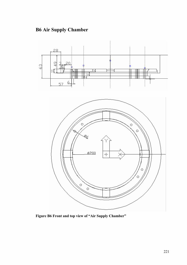
B6 Air Supply Chamber

F

igure
B6 Front and top view of “Air Supply Chamber”
221

Appendix C

Sample CFX Program This run of the CFX-5.6 Solver started at 10:0:4 on 28 Jan 2004 by user DShanmugam on IRIS-ABQHYMCMXX (intel_p3_winnt5.1) using the command: C:\CFX\CFX-5.6\bin\5.6\perllib\cfx5solve.pl -stdout-comms -batch -ccl– Using the CFX-5 Solver optimised for the winnt architecture from C:\CFX\CFX-5.6\bin\5.6\winnt\solver-pvm.exe. Setting up CFX-5 Solver run... +-------------------------------------------------------------------+ | | | CFX Command Language for Run | | | +-------------------------------------------------------------------+ LIBRARY: MATERIAL: Water at 25 C Option = Pure Substance Thermodynamic State = Liquid Long Name = Water (saturated liquid) at 25 C PROPERTIES: Option = General Fluid Molar Mass = 18.02 [kg kmol^-1] Density = 1000 [kg m^-3] Speed Of Sound = 1496 [m s^-1] Dynamic Viscosity = 9.4e-006 [kg m^-1 s^-1] Specific Heat Capacity = 4181.7 [J kg^-1 K^-1] Thermal Conductivity = 0.0193 [W m^-1 K^-1] Thermal Expansivity = 0.000257 [K^-1] Absorption Coefficient = 1 [m^-1] Scattering Coefficient = 0 [m^-1] Refractive Index = 1.0 [m m^-1] Reference Pressure = 1 [atm] Reference Temperature = 25 [C] Reference Specific Enthalpy = -1.58664e+007 [J kg^-1] Reference Specific Entropy = 3882.25 [J kg^-1 K^-1] Density Depends On = Temperature Maximum Absolute Pressure = 1e+007 [Pa] Maximum Temperature = 300 [K] Minimum Absolute Pressure = 1000 [Pa] Minimum Temperature = 100 [K] SPECIFIC HEAT CAPACITY: NASA Coefficient List = 2.67215, 0.00305629, -8.73026e-007, 1.201e-10, -6.39162e-015, -29899.2, 6.86282, 3.38684, 0.00347498, -6.3547e-006, 6.96858e-009, -2.50659e-012, -30208.1, 2.59023 Option = NASA Format Temperature Limit List = 300 [K] END END END

222

MATERIAL: nitrogen Option = Pure Substance Thermodynamic State = Gas PROPERTIES: Absorption Coefficient = 1 [m^-1] Density = 1.25 [kg m^-3] Density Depends On = Temperature Dynamic Viscosity = 1.77e-005 [kg m^-1 s^-1] Maximum Absolute Pressure = 1e+007 [Pa] Maximum Temperature = 300 [K] Minimum Absolute Pressure = 1000 [Pa] Minimum Temperature = 100 [K] Molar Mass = 28.01 [kg kmol^-1] Option = General Fluid Reference Pressure = 1 [atm] Reference Specific Enthalpy = -25896.4 [J kg^-1] Reference Specific Entropy = 6745.4 [J kg^-1 K^-1] Reference Temperature = 0 [C] Refractive Index = 1.0 [m m^-1] Scattering Coefficient = 0 [m^-1] Specific Heat Capacity = 1040 [J kg^-1 K^-1] Thermal Conductivity = 0.0259 [W m^-1 K^-1] Thermal Expansivity = 0.00366 [K^-1] END END END EXECUTION CONTROL: PARALLEL HOST LIBRARY: END PARTITIONER STEP CONTROL: Runtime Priority = Standard MEMORY CONTROL: Memory Allocation Factor = 1 END PARTITIONING TYPE: MeTiS Type = k-way Option = MeTiS Partition Size Rule = Automatic END END RUN DEFINITION: Definition File = icejet28.def Run Mode = Full END SOLVER STEP CONTROL: Runtime Priority = Standard EXECUTABLE SELECTION: Double Precision = Off Use 64 Bit = Off END MEMORY CONTROL: Memory Allocation Factor = 1 END PARALLEL ENVIRONMENT: Option = Serial Parallel Mode = PVM END END END

223

FLOW: SOLUTION UNITS: Angle Units = [rad] Length Units = [m] Mass Units = [kg] Solid Angle Units = [sr] Temperature Units = [K] Time Units = [s] END INITIALISATION: Option = Automatic INITIAL CONDITIONS: STATIC PRESSURE: Option = Automatic with Value Relative Pressure = 1 [atm] END END END EXPERT PARAMETERS: transient initialisation override = t END OUTPUT CONTROL: BACKUP RESULTS: Backup Results 1 Option = Selected Variables Output Variables List = Temperature END TRANSIENT RESULTS: Transient Results 1 Option = Minimal Output Boundary Flows = All Output Variable Operators = All Output Variables List = Temperature Time List = 0.01 [s] END TRANSIENT STATISTICS: Transient Statistics 1 Option = Minimum Output Variables List = Temperature END END SOLVER CONTROL: ADVECTION SCHEME: Option = High Resolution END CONVERGENCE CONTROL: Maximum Number of Coefficient Loops = 100 END CONVERGENCE CRITERIA: Residual Target = 0.0001 Residual Type = RMS END EQUATION CLASS: continuity ADVECTION SCHEME: Option = High Resolution END TRANSIENT SCHEME: Option = Second Order Backward Euler END END EQUATION CLASS: energy ADVECTION SCHEME: Option = Second Order Central Difference END

224

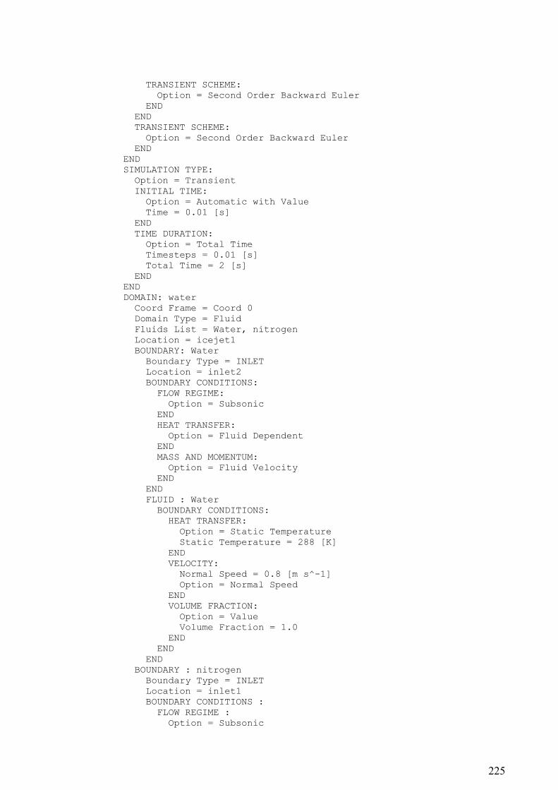
TRANSIENT SCHEME: Option = Second Order Backward Euler END END TRANSIENT SCHEME: Option = Second Order Backward Euler END END SIMULATION TYPE: Option = Transient INITIAL TIME: Option = Automatic with Value Time = 0.01 [s] END TIME DURATION: Option = Total Time Timesteps = 0.01 [s] Total Time = 2 [s] END END DOMAIN: water Coord Frame = Coord 0 Domain Type = Fluid Fluids List = Water, nitrogen Location = icejet1 BOUNDARY: Water Boundary Type = INLET Location = inlet2 BOUNDARY CONDITIONS: FLOW REGIME: Option = Subsonic END HEAT TRANSFER: Option = Fluid Dependent END MASS AND MOMENTUM: Option = Fluid Velocity END END FLUID : Water BOUNDARY CONDITIONS: HEAT TRANSFER: Option = Static Temperature Static Temperature = 288 [K] END VELOCITY: Normal Speed = 0.8 [m s^-1] Option = Normal Speed END VOLUME FRACTION: Option = Value Volume Fraction = 1.0 END END END BOUNDARY : nitrogen Boundary Type = INLET Location = inlet1 BOUNDARY CONDITIONS : FLOW REGIME : Option = Subsonic

225

END HEAT TRANSFER : Option = Fluid Dependent END MASS AND MOMENTUM : Option = Fluid Velocity END END FLUID: liquid nitrogen BOUNDARY CONDITIONS: HEAT TRANSFER: Option = Static Temperature Static Temperature = 173 [K] END VELOCITY: Normal Speed = 0.6 [m s^-1] Option = Normal Speed END VOLUME FRACTION: Option = Value Volume Fraction = 1.0 END END END END

BOUNDARY: out Boundary Type = OUTLET Location = outlet BOUNDARY CONDITIONS: FLOW REGIME: Option = Subsonic END MASS AND MOMENTUM: Option = Static Pressure Relative Pressure = 1e+005 [Pa] END END END BOUNDARY: water Default Boundary Type = WALL

Location = Solid 1.1,Solid 1.2,Solid 1.3,Solid 1.4,Solid 1.5,Solid 1.6

BOUNDARY CONDITIONS: HEAT TRANSFER: Option = Adiabatic END WALL INFLUENCE ON FLOW: Option = Free Slip END END WALL CONTACT MODEL: Option = Use Volume Fraction END END DOMAIN MODELS: BUOYANCY MODEL: Buoyancy Reference Density = 1000 [kg m^-3] Gravity X Component = 0 [m s^-2] Gravity Y Component = 0 [m s^-2] Gravity Z Component = 9.81 [m s^-2] Option = Buoyant

226

END DOMAIN MOTION: Option = Stationary END REFERENCE PRESSURE: Reference Pressure = 1e+05 [Pa] END END FLUID MODELS: COMBUSTION MODEL: Option = None END HEAT TRANSFER MODEL: Option = Thermal Energy END THERMAL RADIATION MODEL: Option = None END TURBULENCE MODEL: Homogeneous Model = On Option = Laminar END END FLUID PAIR: Water | liquid nitrogen INTERPHASE HEAT TRANSFER: Option = Two Resistance FLUID1 INTERPHASE HEAT TRANSFER: Option = Zero Resistance END FLUID2 INTERPHASE HEAT TRANSFER: Option = Ranz Marshall END END INTERPHASE TRANSFER MODEL: Option = Particle Model END MASS TRANSFER: Option = Phase Change PHASE CHANGE MODEL: Option = Thermal Phase Change Saturation Temperature = 273 [K] END END MOMENTUM TRANSFER: DRAG FORCE: Option = Schiller Naumann END END END FLUID: Water FLUID MODELS: FLUID BUOYANCY MODEL: Option = Density Difference END MORPHOLOGY: Mean Diameter = 120 [micron] Option = Dispersed Fluid END END END

227

FLUID: nitrogen FLUID MODELS: FLUID BUOYANCY MODEL: Option = Density Difference END MORPHOLOGY: Option = Continuous Fluid END END END MULTIPHASE MODELS: Homogeneous Model = Off FREE SURFACE MODEL: Option = None END END END END COMMAND FILE: Version = 5.6 Results Version = 5.6 END

228

development of ice particle formation system for ice jet ... · technology (crc-imst) for...

Documents