development of direct utility avoided cost methodology & model · development of direct utility...

10/31/04, v1

DEVELOPMENT OF DIRECT UTILITY AVOIDED COST

METHODOLOGY & MODEL

Draft October 31, 2004

Prepared for the California Urban Water Conservation Council by A & N Technical Services, Inc.

and Quantec, LLC

10/31/04, v1 ii

Authors’ notes:

1. These chapters presume an understanding of the different perspectives used by the CUWCC MOU and examines methodological issues of avoided costs from a water utility perspective.

2. Chapter 2 provides the methodological review of concepts and theory. Chapter 3 provides the draft proposed method. In this way we separate conceptual issues of methodological approach from the practical questions of how the method should be enacted. We believe this distinction will prove helpful for focusing feedback from the Project Advisory Committee.

3. The draft method proposed in Chapter 3 is inspired by the authors’ experience with system simulation models. The proposed method adheres to the logic used by these models, while attempting to minimize data requirements. Specifically, the method allows utilities to estimate avoided costs that differ by season and, possibly, area. We have attempted to follow a variant of the KISS principle—Keep It Simple, not Stupid.

4. The reader should bear in mind that these methodological chapters are intended to accompany a spreadsheet model that enacts the method, worked examples to illustrate the logic, and a user guide to accompany the spreadsheet.

5. We look forward to your review. Tom Chesnutt Gary Fiske

10/31/04, v1 1

CHAPTER 2: DIRECT UTILITY AVOIDED COSTS METHODOLOGY—CONCEPTS AND THEORY Water utilities who confront sudden changes in their cost structure have naturally turned

to the question of how they can reduce the incidence of future costs. The question of how

to avoid future cost lies at the heart of avoided cost analysis. By analyzing the direct costs

that utilities can avoid via demand reduction, water utilities define the benefits produced

by conservation programs.

Avoided Costs and Demand Management

Different conservation programs can have different types of effects on demand. Water

agencies can use conservation programs to help manage water demand—throughout the

year, during periods of seasonal peak demand, and in specific geographical zones. An

analysis of utility avoided costs can guide the development of conservation programs that

produce the greatest benefit (as measured by avoided costs).

Goal 1-Reduce average system load. Conservation programs can reduce total annual water use, that is, reduce average day demand. This goal may be particularly appropriate if the agency faces a supply source constraint that could necessitate the importing or purchasing relatively costly supplies. Demand management can help utilities avoid these costs. Goal 2-Reduce peak system load. A related goal for a water agency in implementing conservation programs can be to reduce seasonal water demand. This objective may be particularly appropriate for agencies facing costly capacity expansion—because capacity costs are often driven by peak capacity requirements. Again, these costs may be avoidable through effective demand management. Goal 3-Reduce system spatial diseconomies. Finally, agencies may want to target difficult-to-serve areas, with targeted water conservation programs. Agencies should also recognize, however, that customers willing to pay more for expensive types of water service are communicating a willingness to pay for additional investments to provide additional water service. Rather than a failing of conservation, customer preferences for additional water service should be viewed as a form of desirable two-way price signaling.

10/31/04, v1 2

In this chapter we explain the methodological background required to implement an

analysis of utility avoided costs. The step-by-step method is set forth in Chapter 3 and

embeds the above three goals. Many avoided cost analyses focus solely on quantifying

the value, in avoided costs, of overall reductions in demand (average system load.) This

type of simplistic approach can lead to incorrect conclusions about the desirability of

different kinds of conservation programs. The method proposed in Chapter 3 permits

utilities to consider differences in average avoided costs that pertain to peak demand

reduction and/or spatial cost differences.

This chapter is divided into several distinct sections. The following section defines some

basic terms used in cost analysis. This is followed by a basic definition of avoided costs

and a brief explanation of its applications in utility cost analysis. The following section

separates avoided costs by time—short run avoided costs and long run avoided costs. The

following sections provide explanations of some methodologies that have been used in a

water utility setting to quantify the avoided costs. The reader should note that these

methods focus on quantifying the avoided cost of reductions in average demand load.

Chapter 3 builds on these approaches to provide an integrated method that incorporates

differences in seasonal demand reduction and spatial cost differences.

COST CONCEPTS Understanding the costing methods required to estimate a utility’s avoided costs involves

several basic issues. First, the distinction between fixed and variable costs, which is key

to many costing methods, depends entirely on the time period under consideration.

Second, assigning cost responsibility requires a distinction between assignable and joint

costs. Third, data quality and availability will limit cost analysis. This section defines

these basic cost concepts and explains their relevance to costing methods.

Fixed versus Variable Costs: Many costing methods identify costs of water service as

either fixed or variable based on accounting expenditures. Fixed costs are expenditures

that remain the same, regardless of the volume of water produced. Because large up-front

capital costs are required to build capacity for meeting demand, some traditional costing

10/31/04, v1 3

methods classify all system expansion costs as fixed and refer to these costs as “demand”

costs. Variable costs, also called “commodity costs,” are expenditures that vary directly

with the volume of water produced or consumed; variable costs include, for example,

purchased-water, electrical, and chemical costs. Marginal costing methods recognize that

the dividing line between fixed and variable depends on the period of time used for the

analysis. In the long run, fixed capital expenditures can and do change, thus becoming

“avoidable.”

Assignable versus Joint Costs: If all costs could be easily, accurately, and cheaply

assigned to specific utility functions, cost-causation would be straightforward. Some

costs of water supply are considered “joint” costs because they reflect joint functions. As

an example, providing flow capacity sufficient for fire protection simultaneously (or

jointly) provides capacity that can be used for any other instantaneous high-flow use.

Similarly, providing capacity for peak periods will necessarily provide capacity for

nonpeak periods. Joint costs complicate the task of cost analysis.

Data Issues: Costing methods use, and are limited by, accounting data generated in the

day-to-day operations of the water utility. The quality and availability of these data also

affect the accuracy and applicability of avoided-cost methods. Much of the water supplier

cost accounting data, for example, is not allocated by utility function—supply, storage,

treatment, and conveyance. By improving the process of defining and collecting

accounting-cost measures, better decisions can be made using even simple methods.

10/31/04, v1 4

DEFINITION AND HISTORY OF AVOIDED COST METHODS An important starting point in the discussion of using avoided cost methods to value

conserved water is the proper definition of marginal costs. “Marginal” costs refer to the

cost of producing (or not producing) another unit of water supply. Marginal costs taken

for an increment of supply are often referred to as “incremental” costs. In estimating

marginal costs, a central issue is where the next increment of supply will come from and

what it will cost. A variety of supply options with different capacity and cost

consequences may be available. The identification and quantification of future resource

alternatives lies at the heart of water agency planning. Existing water supply/management

plans are a good place to start to determine baseline assumptions about the current set of

resource alternatives to which an agency is committed.

The Appropriate Time Horizon: Calculating marginal cost involves projecting capacity

costs, operating costs, and water demand over a specified time horizon. These projections

may require data on the price elasticity of demand, anticipated changes in technology,

and the prices of inputs required to provide water service.

Selecting the time horizon directly affects the estimation of marginal capacity cost (long-

run marginal cost) and the marginal operating cost (short-run marginal cost). The length

of the time horizon or planning period affects both the cost numerator and the output

denominator in calculating marginal cost.

Sometimes a shorter time period has been chosen out of a misplaced desire for precision

in estimating marginal costs. Though it is often true that shorter time horizons lend

themselves to more precise cost and demand forecasts, precision should not be

confused with accuracy. Forecasts over long time horizons may contain fewer known

and more estimated quantities. These longer term forecasts can be more accurate, because

they contain a broader set of alternatives, while necessarily being less precise. The choice

of the time horizon also must take into account the span of time required to implement

cost-effective changes in the mix, capacity or availability of resources. Most water

10/31/04, v1 5

agencies define a “time horizon” for planning purposes; this is a good working

assumption until a longer or shorter horizon can be justified by analytic considerations.

Avoided cost methods have a long history of development in the economic literature and

have been successfully applied to problems of public utility planning.1 The historical

evolution of traditional costing in the water industry drew heavily from methods

developed for other public utility industries. In the energy and telecommunications

industries, where most utilities are subject to economic regulation, average-cost pricing

prevailed until roughly the 1980s. Marginal-cost methods have gained some acceptance

in the realm of public utility regulation. In fact, the Public Utility Regulatory Policies

Act (PURPA) of 1979 required the larger electric and gas utilities to consider these

marginal costing methods.

The concept of marginal costs has also been extended beyond direct production costs.

They should be thought of as inclusive of all marginal opportunity costs, including

marginal connection costs and marginal environmental costs.2 We begin with a review of

the key literature on marginal costing applied to water utilities. The reader should note

that this literature focuses on marginal production and delivery costs of water utility

service.

MARGINAL COSTS—TWO COMPONENTS Two important components of marginal cost are the change in operating costs caused by

a change in the use of existing capacity (short-run marginal operating cost), and the cost

of expanding capacity (long-run marginal capacity cost).

1 In fact, some of the early work on marginal cost methods for public utilities was focused specifically on hydroelectric reservoirs. See Massé, P. 1944, Application des probabilités en chaîne à l’hydrologie statistique et au jeu des réservoirs. Paris. or Boiteux, M., 1949, “La tarification des demandes en pointe,” Revue Générale de l’Electricité, 58, 321-40. 2 See for example, R.C. Griffin, 2001, “Effective Water Pricing,” Journal of the American Water Resources Association.

10/31/04, v1 6

Short-run marginal operating costs reflect the cost consequences during time periods

in which some inputs are fixed. Short-run marginal costs are comprised mostly of

variable operating costs

Long-run marginal capacity costs extend to time periods far enough into the future to

be changed by system and resources planning. Long-run marginal costing methods

can identify costs that can be avoided through more efficient use or nonuse

(conservation). Because the long-run concept of marginal costs (1) extends into the

future, and (2) reflect all future alternatives, estimation methods must deal with more

uncertainty. Total long run marginal costs include both the short-run operating costs and the long-run

capacity expansion/contraction costs.

Marginal Operating Cost

A water agency’s marginal operating cost (MOC) in any time period is a function of the

system components whose operation would be cut back in response to a small reduction

in that period’s demand. These components are said to be operating ‘on the margin’. In

real time, the precise supplies, reservoirs, and treatment and conveyance facilities that

would be cut back may be determined by a complex mix of economic, operational,

regulatory, and other factors. The key is then to estimate the likelihood of each

component being on the margin in each time period.

The literature includes many methods to estimate a water agency’s marginal operating

cost (MOC). Following are brief discussions of two of these.

A Simple Method:

One technique used to calculate MOC is to forecast the annual operating expenses for the

first year that a capacity increment is anticipated to become operational, and then divide

that annual cost estimate by the forecast revenue-producing output for the same year

10/31/04, v1 7

(Hanke, 1981)3. When operating costs can be predictably forecast, this technique can be

extended over multiple years. The forecast annual operating expenses over the entire

planning period in which the capacity increment is anticipated to become operational are

divided by the forecast revenue-producing output for the same time period (Hanke,

1978). Water systems exhibiting significant seasonal operating cost differences—due to

purchased water prices or electrical power expenses—can adapt this technique to a

seasonal basis4.

Illustration: Table 2-2 illustrates the two calculations of average operating cost. The example assumes that a new treatment plant is operational in Year 1. The projected annual operating expenses and revenue-producing output of a new facility are provided in the table. The first method, using data only from Year 1, generates an average operating cost of $0.47 per CCF. The second method, using data from Years 1 through 5, generates an annual estimate of average operating cost that increases to $0.50 per CCF. Table 2-2. Calculation of Average Operating Cost - Hanke Method

Description Year 1 Year 2 Year 3 Year 4 Operating Expense (millions of dollars) $4.343 $4.3760 $4.4370 $4.7150Revenue-Producing Water(CCF) 9,288,311 9,330,170 9,372,302 9,414,711Average Operating Cost ($/CCF) $0.468 $0.469 $0.473 $0.501

The primary advantage of this technique is its low data requirements. The primary

disadvantage is that, strictly speaking, this technique produces an estimate of average, not

marginal operating cost. Producing an estimate of marginal operating cost can be

performed using additional data and readily available statistical methods.

A Regression-based Method: A recent study by Bishop and Weber (1996) used three

years of monthly historical cost data to develop statistical estimates of marginal operating

costs. This study allows comparison of average operating cost methods with methods that

control for other factors. In models for seven water agencies, this study found total

marginal operating costs to range from $0.05 to $0.20 per CCF. (An eighth agency

3The revenue producing output is used as a way to adjust for losses in the water system. Since most water systems exhibit some level of losses, more than one gallon of water must be produced in order to deliver one gallon. 4Other MOC methods can be found in Table 4-1 of Beecher and Mann, 1991.

10/31/04, v1 8

purchased treated water at a marginal cost of $0.59 per CCF with an additional two cents

required for electrical distribution costs.) Table C-3 provides a comparison of the average

versus marginal operating costs derived from the study. As can be seen, the regression-

based estimates of marginal operating costs are less than the average operating costs.5

Water agencies interested in replicating this approach would collect a set of consistent

time series on operating costs, production volume (adjusted for system loss), and other

factors that can influence operating costs (turbidity levels or deterministic time trends, for

example.) Interested readers should refer to the original study for additional details on

model specification and estimation.

Analysts who are put off by what may seem as an intimidating methodology should

consider a direct application of this approach. Regression-approaches seek to control for

external factors that can change operating costs other than changes in volume. The same

question can be put directly to operators in the field: “How would your (electrical,

chemical, or other operating) budget change with specified changes in revenue-producing

output volume?” Compilation of this directly assayed information should yield the same

answers produced by a well controlled statistical study.

Marginal Capacity Costs Most of the marginal capacity cost (MCC) estimation techniques used in water system

cost analysis are variations of two basic MCC approaches: (1) the avoided cost due to

5 Since a regression model can be specified to estimate an “average” operating cost, it is wrong to attribute the difference between the two estimates solely to method. The regression-based method yielded a lower estimate because the model was able to control for the other influences upon operating costs. A simple average, by contrast, forces all variation in operating costs to be explained (caused) by output. Consider the model:

ntityoducingQuavenuebaratingCostMonthlyOpe PrRe•+= Where a and b are the coefficients to be estimated. If the coefficient a is constrained to be zero, the above regression equation will produce an estimate of b equivalent to an average operating cost. If the fixed cost coefficient a is not constrained and takes on a positive value, the estimated coefficient b will necessarily be less than the average operating cost.

10/31/04, v1 9

system expansion deferral (a time shift) and (2) the Average Incremental Cost (AIC) used

to estimate a change in capacity requirement (downsizing).6

A common thread running through the alternative approaches is that the MCC results are

very sensitive to the specification of the cost numerator and the quantity denominator.

The application of any long run marginal costing method requires analysts to address

several future cost issues:

1) Projections of demand—consistent with system planning—are essential for determining both the denominator in the cost function and to identify demand levels that trigger the need for incremental capacity7.

2) Cost projections to determine the numerator (the forecast of costs over the

capital project life). 3) Inflation and discount rates should be consistent with those used in the

planning process of the water agency. Sensitivity analyses should be conducted allowing these key assumptions to vary.8

Depending upon the method employed, other information (such as the capacity service

lives, planned operating characteristics, and costs of other alternatives such as water

purchases or reclaimed water) may be required.

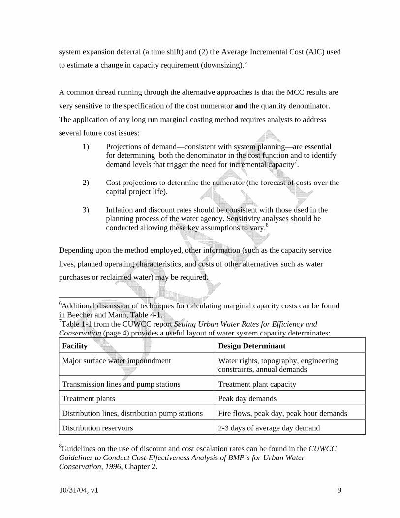
6Additional discussion of techniques for calculating marginal capacity costs can be found in Beecher and Mann, Table 4-1. 7Table 1-1 from the CUWCC report Setting Urban Water Rates for Efficiency and Conservation (page 4) provides a useful layout of water system capacity determinates:

Facility Design Determinant

Major surface water impoundment Water rights, topography, engineering constraints, annual demands

Transmission lines and pump stations Treatment plant capacity

Treatment plants Peak day demands

Distribution lines, distribution pump stations Fire flows, peak day, peak hour demands

Distribution reservoirs 2-3 days of average day demand 8Guidelines on the use of discount and cost escalation rates can be found in the CUWCC Guidelines to Conduct Cost-Effectiveness Analysis of BMP’s for Urban Water Conservation, 1996, Chapter 2.

10/31/04, v1 10

We begin the methodological review of capacity costing with a brief description and

discussion of each of these MCC techniques. The reader should note that the following

methodological discussion, though focussed on techniques addressing the MCC of

average system load reductions, provides the building blocks for the specific method

proposed in Chapter 3.

Marginal Capacity Cost as a Deferred Cost: As explicated by Turvey9, this approach

expresses MCC as either the cost incurred by an acceleration in growth of demand, or as

the cost avoided by a deceleration of demand. A plan for system expansion is taken as a

given, and only the timing of that expansion is varied; plans for system expansion are not

re-optimized, only rescheduled. The original Turvey method examined the savings

associated with slowing down system expansion through conservation. The cost

numerator was formed by the change in the present value of capacity expenditures by

moving the capacity increment forward into the future. The usage denominator was the

annual change in demand that allowed the postponement of the capital facility. The

original Turvey method focused on the change in cost associated with a postponement or

acceleration of the construction period.

9 Turvey, R. (1976) “Analyzing the Marginal Cost of Water Supply,” Land Economics, 52, 158-168, May 1976.

10/31/04, v1 11

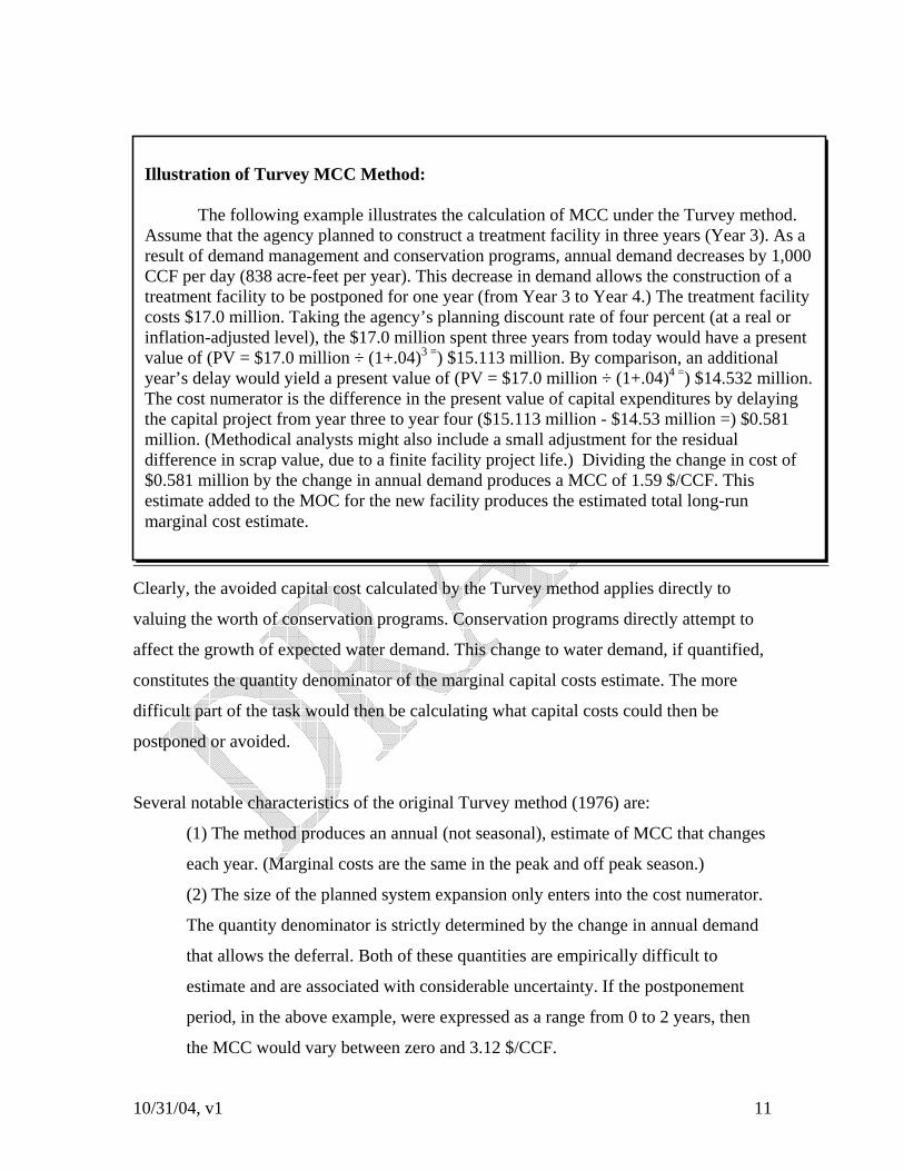
Clearly, the avoided capital cost calculated by the Turvey method applies directly to

valuing the worth of conservation programs. Conservation programs directly attempt to

affect the growth of expected water demand. This change to water demand, if quantified,

constitutes the quantity denominator of the marginal capital costs estimate. The more

difficult part of the task would then be calculating what capital costs could then be

postponed or avoided.

Several notable characteristics of the original Turvey method (1976) are:

(1) The method produces an annual (not seasonal), estimate of MCC that changes

each year. (Marginal costs are the same in the peak and off peak season.)

(2) The size of the planned system expansion only enters into the cost numerator.

The quantity denominator is strictly determined by the change in annual demand

that allows the deferral. Both of these quantities are empirically difficult to

estimate and are associated with considerable uncertainty. If the postponement

period, in the above example, were expressed as a range from 0 to 2 years, then

the MCC would vary between zero and 3.12 $/CCF.

Illustration of Turvey MCC Method: The following example illustrates the calculation of MCC under the Turvey method. Assume that the agency planned to construct a treatment facility in three years (Year 3). As a result of demand management and conservation programs, annual demand decreases by 1,000 CCF per day (838 acre-feet per year). This decrease in demand allows the construction of a treatment facility to be postponed for one year (from Year 3 to Year 4.) The treatment facility costs $17.0 million. Taking the agency’s planning discount rate of four percent (at a real or inflation-adjusted level), the $17.0 million spent three years from today would have a present value of (PV = $17.0 million ÷ (1+.04)3 =) $15.113 million. By comparison, an additional year’s delay would yield a present value of (PV = $17.0 million ÷ (1+.04)4 =) $14.532 million. The cost numerator is the difference in the present value of capital expenditures by delaying the capital project from year three to year four ($15.113 million - $14.53 million =) $0.581 million. (Methodical analysts might also include a small adjustment for the residual difference in scrap value, due to a finite facility project life.) Dividing the change in cost of $0.581 million by the change in annual demand produces a MCC of 1.59 $/CCF. This estimate added to the MOC for the new facility produces the estimated total long-run marginal cost estimate.

10/31/04, v1 12

(3) The Turvey MCC gets larger as the system gets closer to its capacity limitations and is zero otherwise. Since water projects involve large discrete changes in system capacity, the resulting Turvey marginal cost estimates could be volatile.

(4) The Turvey MCC focuses only on the next capacity increment, ignoring the

cost consequences of subsequent increments.

Different variants of the Turvey approach have been proposed:

(1) To produce a seasonal estimate of MCC, Hanke (1975) suggested categorizing cost data into facility costs designed to meet peak demands and system costs designed to meet average demands. Hanke (1981) implemented a seasonal variant of a Turvey avoided capital cost by disaggregating cost and consumption data into peak and off-peak periods. (2) Several applications have stressed quantifying the demand expected in the future and linking changes in this expected demand to the corresponding sizes of the deferrable facilities. (For an illustration, see Hanke, 1981). These variants of the Turvey approach will use the same numerator (the difference in the present value costs of two differently timed but otherwise identical system expansions) while substituting the planned usable facility capacity (that matches the avoided demand) into the denominator. The denominator is also adjusted downward to account for the effect of system loss; due to distribution leaks, more than one gallon must be produced to deliver one gallon of water.

(3) Several variants of the Turvey method use an averaging of the marginal cost over several years for different rationales:

• as the long run consistent strategy that results when an administrative feasibility constraint is included in an optimal planning framework (Dandy, 1984),

• to produce a consistent price signal for long-term decision making (Boiteux, 1959), and

• as a more appropriate tradeoff between short-run allocative efficiency (efficient use of existing capacity) and long-run resource efficiency(efficient capacity-sizing decisions) (Mann et al., 1980).

The original Turvey method (1976) is direct, relatively straightforward, and requires only

data available in the existing water system plan. As such, it is easily interpretable as the

direct cost of additional (or avoided) water use. Though directly appropriate for

assigning value to conservation (demand-side management), strict implementation of the

10/31/04, v1 13

original Turvey method has several shortcomings: it does not reflect the higher cost of

using water during peak periods (without an additional seasonal allocation step), it

becomes erratic when capacity increments are lumpy, and it does not look beyond the

next capacity increment. Other methods for calculating marginal capacity costs have also

been proposed.

Marginal Capacity Cost as an Average Incremental Cost: The Average Incremental Cost

(AIC) approach for estimating MCC involves the annualization of incremental cost. The

AIC approach first involves calculating annualized capacity cost (K), which is defined as

the annual payment, over the useful service life of the new capacity (n), required to

recover both financing costs and the additional capacity costs:

1]1[]1[

−++⋅⋅

≡ n

n

iiiCK

where: K = total annualized incremental capacity costs, C = total capital expenditure required, N = useful service life of the capacity increment, and i = appropriate financing (interest) rate.

“K” must be calculated for each system function (that is, source development,

transmission, treatment, etc.) in which a capacity increment is planned, since service lives

will vary across these functions. “K” can be disaggregated into peak/off-peak

components.

The output (quantity) denominator is based on the designed annual capacity (annual firm

yield). The planned capacity, however, should be adjusted to account for losses due to

leakage in the system. System losses mean that more than one gallon must be produced to

deliver one gallon to the customer. For example, a system loss of 10 percent implies that

1.11 gallons must be produced for each gallon delivered. The output denominator can be

expressed as revenue-producing annual capacity (annual planned delivery capacity

averaged over the life of the plant)10

10Some AIC calculations take the accounting an additional step, separately accounting for the capacity that is used and the capacity that is held in reserve. Analysts should avoid using “expected capacity utilization” as the output denominator; this sends the exact wrong short run signal. (Since the expected utilization is low immediately after

10/31/04, v1 14

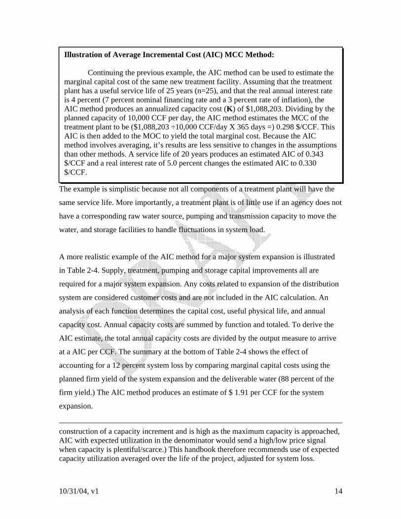
The example is simplistic because not all components of a treatment plant will have the

same service life. More importantly, a treatment plant is of little use if an agency does not

have a corresponding raw water source, pumping and transmission capacity to move the

water, and storage facilities to handle fluctuations in system load.

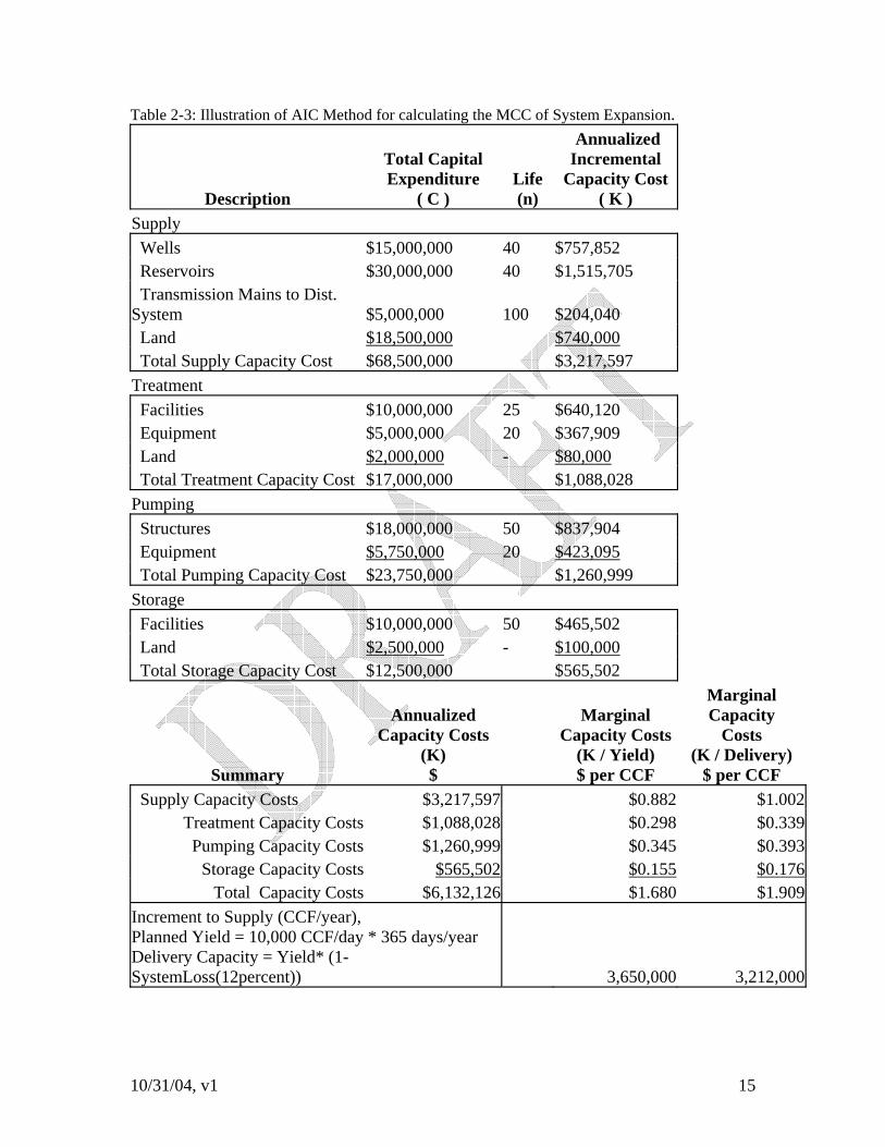
A more realistic example of the AIC method for a major system expansion is illustrated

in Table 2-4. Supply, treatment, pumping and storage capital improvements all are

required for a major system expansion. Any costs related to expansion of the distribution

system are considered customer costs and are not included in the AIC calculation. An

analysis of each function determines the capital cost, useful physical life, and annual

capacity cost. Annual capacity costs are summed by function and totaled. To derive the

AIC estimate, the total annual capacity costs are divided by the output measure to arrive

at a AIC per CCF. The summary at the bottom of Table 2-4 shows the effect of

accounting for a 12 percent system loss by comparing marginal capital costs using the

planned firm yield of the system expansion and the deliverable water (88 percent of the

firm yield.) The AIC method produces an estimate of $ 1.91 per CCF for the system

expansion.

construction of a capacity increment and is high as the maximum capacity is approached, AIC with expected utilization in the denominator would send a high/low price signal when capacity is plentiful/scarce.) This handbook therefore recommends use of expected capacity utilization averaged over the life of the project, adjusted for system loss.

Illustration of Average Incremental Cost (AIC) MCC Method: Continuing the previous example, the AIC method can be used to estimate the marginal capital cost of the same new treatment facility. Assuming that the treatment plant has a useful service life of 25 years (n=25), and that the real annual interest rate is 4 percent (7 percent nominal financing rate and a 3 percent rate of inflation), the AIC method produces an annualized capacity cost (K) of $1,088,203. Dividing by the planned capacity of 10,000 CCF per day, the AIC method estimates the MCC of the treatment plant to be ($1,088,203 ÷10,000 CCF/day X 365 days =) 0.298 $/CCF. This AIC is then added to the MOC to yield the total marginal cost. Because the AIC method involves averaging, it’s results are less sensitive to changes in the assumptions than other methods. A service life of 20 years produces an estimated AIC of 0.343 $/CCF and a real interest rate of 5.0 percent changes the estimated AIC to 0.330 $/CCF.

10/31/04, v1 15

Table 2-3: Illustration of AIC Method for calculating the MCC of System Expansion.

Description

Total Capital Expenditure

( C )

Life (n)

Annualized Incremental

Capacity Cost ( K )

Supply Wells $15,000,000 40 $757,852 Reservoirs $30,000,000 40 $1,515,705 Transmission Mains to Dist. System $5,000,000 100 $204,040 Land $18,500,000 $740,000 Total Supply Capacity Cost $68,500,000 $3,217,597 Treatment Facilities $10,000,000 25 $640,120 Equipment $5,000,000 20 $367,909 Land $2,000,000 - $80,000 Total Treatment Capacity Cost $17,000,000 $1,088,028 Pumping Structures $18,000,000 50 $837,904 Equipment $5,750,000 20 $423,095 Total Pumping Capacity Cost $23,750,000 $1,260,999 Storage Facilities $10,000,000 50 $465,502 Land $2,500,000 - $100,000 Total Storage Capacity Cost $12,500,000 $565,502

Summary

Annualized Capacity Costs

(K) $

Marginal Capacity Costs

(K / Yield) $ per CCF

Marginal Capacity

Costs (K / Delivery)

$ per CCF Supply Capacity Costs $3,217,597 $0.882 $1.002

Treatment Capacity Costs $1,088,028 $0.298 $0.339 Pumping Capacity Costs $1,260,999 $0.345 $0.393

Storage Capacity Costs $565,502 $0.155 $0.176 Total Capacity Costs $6,132,126 $1.680 $1.909

Increment to Supply (CCF/year), Planned Yield = 10,000 CCF/day * 365 days/year Delivery Capacity = Yield* (1-SystemLoss(12percent)) 3,650,000 3,212,000

10/31/04, v1 16

The average costs for additional capacity increments can be used to calculate a

downsizing avoided cost attributable to reduced demand. This relatively straight forward

process involves comparing two average incremental capacity costs—the AIC designed

without the effect of conservation programs and the AIC of a system designed with

conservation. Though the calculation of avoided capacity costs due to downsizing is less

common, it is mentioned here for several reasons. First, it is a valid method that has

found use in the water industry. Second, these costing methods also provide the basis for

the determination of a “good” price signal to be provided by water rates. Last, calculation

of average incremental costs by function can serve as a useful benchmark for other

costing methods.

CONCLUSION All of the foregoing approaches shed light on the issues that must be addressed in

estimating marginal costs. However, none of them suffices as a method to be used by

utilities given real-world resource and analytical constraints. Chapter 3 presents an

approach that incorporates the requisite analytical rigor in an approach that is usable by

and adaptable to the needs of different water utilities.

10/31/04, v1 1

CHAPTER 3: DRAFT METHOD FOR ESTIMATING

DIRECT UTILITY AVOIDED COSTS

The estimation of a water utility’s avoided supply costs begins with baseline assumptions

about the future supply and infrastructure investments that would be made and the

manner in which the system would be operated in the absence of conservation. The

question that must then be answered is how one or both of these would change due to the

demand reductions that occur as a result of conservation.

Changes in system operations may result in reduced costs of production that vary as a

function of the quantity of water produced. These marginal operating costs include power

and chemicals, and any other costs which vary directly with the volume of water

delivered. These are often called ‘short-run avoided costs’. As long as a conservation

program causes net demand reductions, it almost always avoids this type of cost.

Over the long run, it is assumed that not only could marginal operating costs be avoided

because of reduced production levels, but that the ability to downsize or defer

investments in new supply and/or infrastructure could result in additional ‘long-run

avoided costs’—the marginal capacity cost.

In order for water utilities to properly estimate direct avoided supply costs, they must

carefully distinguish between and account for both types of costs. To the extent that they

differ significantly across seasons or as a function of weather or hydrology, those

differences must be reflected.

Baseline Assumptions

To begin the analysis, the utility must provide the following baseline information. Each

of these is essential to the computation of avoided costs.

10/31/04, v1 2

• Planning horizon. Through what year does the planning period extend?

• Escalation and discount rates. How quickly will different types of

costs increase over time, and what rate should be used to estimate the present value of time series of avoided costs?

• Financing assumptions. Over what period and at what interest rate

will capital investments be financed?

• Analytical time period. Depending on the particular utility characteristics, it may or may not be important to distinguish between avoided costs in different seasons or, perhaps, months. If a seasonal distinction is to be made, the computation will need to know how many days are in each season (see below).

• Demand forecast. What is the demand forecast over the planning

horizon for the time periods selected above. The demand forecast must reflect expected ongoing conservation—the water savings that will occur anyway (“passive conservation” without any additional utility expenditures on conservation programs (“active conservation”).

• Existing system components. Key components of the existing supply and delivery system must be enumerated, including supply,11 storage, treatment, and conveyance12, along with the marginal operating costs associated with each. While ‘conveyance’ could include all levels of ‘pumps and pipes’, the system should be summarized as groups of conveyance ‘paths’. Each conveyance path will represent one way of moving supplies to the customer.13 The paths in each category will all have approximately the same marginal operating (i.e. pumping) costs.

• New system components. This includes those additions expected to

be made over the planning horizon. Only those additions which are or may be a function of growing demand need be entered. Thus, for example, additions which are solely for the purpose of meeting regulatory requirements or replacing aging facilities need not be entered. For each new component, the expected on-line date, size, capital cost, fixed annual operating cost (if any), and marginal operating costs will be required.

11 Supply may include water purchases. 12 As used here, the term ‘conveyance’ includes the entire water delivery system from source to customer. 13 Conveyance paths could include treatment plants. See footnote below for caution about not double counting marginal treatment costs.

10/31/04, v1 3

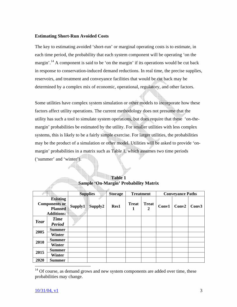
Estimating Short-Run Avoided Costs The key to estimating avoided ‘short-run’ or marginal operating costs is to estimate, in

each time period, the probability that each system component will be operating ‘on the

margin’.14 A component is said to be ‘on the margin’ if its operations would be cut back

in response to conservation-induced demand reductions. In real time, the precise supplies,

reservoirs, and treatment and conveyance facilities that would be cut back may be

determined by a complex mix of economic, operational, regulatory, and other factors.

Some utilities have complex system simulation or other models to incorporate how these

factors affect utility operations. The current methodology does not presume that the

utility has such a tool to simulate system operations, but does require that these ‘on-the-

margin’ probabilities be estimated by the utility. For smaller utilities with less complex

systems, this is likely to be a fairly simple exercise. For larger utilities, the probabilities

may be the product of a simulation or other model. Utilities will be asked to provide ‘on-

margin’ probabilities in a matrix such as Table 1, which assumes two time periods

(‘summer’ and ‘winter’).

Table 1 Sample ‘On-Margin’ Probability Matrix

Supplies Storage Treatment Conveyance Paths

Existing Components or

Planned Additions:

Supply1 Supply2 Res1 Treat1

Treat2 Conv1 Conv2 Conv3

Year Time Period

Summer 2005 Winter Summer 2010 Winter Summer 2015 Winter

2020 Summer 14 Of course, as demand grows and new system components are added over time, these probabilities may change.

10/31/04, v1 4

Winter Summer 2025 Winter Summer 2030 Winter

In some time periods in some years, it may well be that a single supply source is always

expected to be the marginal supply. If so, the entry for that supply would be 100%, with

zero entries for the other supplies. (Since added marginal operating costs may be incurred

treating and/or conveying the water, there will likely also be additional nonzero entries in

these categories.)

On the other hand, for other time periods, multiple supplies (or reservoirs or treatment

plants) may have some likelihood of production cutbacks in response to demand

reductions, depending on weather, hydrology, operating rules, etc. In that case, this

matrix will reflect utility staff’s best estimate of the probabilities that each unit is subject

to cutback in response to conservation-induced savings.

The short-term avoided costs for each time period in each year in the matrix will be

computed as the sum of the products of the marginal operating cost for each system

component and the corresponding probability.15 The short-term avoided costs for

intervening years will be calculated by linear interpolation.

Estimating Marginal Capacity Costs The calculation of marginal capacity costs will be based on the degree to which the need

for each planned addition can be deferred due to conservation-induced demand

reductions. We must distinguish between demand reductions in different periods.

Capacity deferrals due to reductions in peak-period demands. It is assumed that the

primary driver of the need for each planned system addition is peak-period (season,

month) demand. In any future year, the duration of potential deferral for each unit of

15 If a utility includes treatment, and its associated costs, in the conveyance paths, the marginal operating costs for treatment should not be accounted for separately.

10/31/04, v1 5

peak-period savings depends on the rate at which peak-period demand is growing in the

planned on-line year of the addition.

For example, if peak-period demand is projected to be growing at a rate of 2 mgd per

year in the year that a particular addition is scheduled to come on-line, then the maximum

interval that each mgd of peak-period conservation will defer that investment is 0.5 years.

This deferral reduces the present value of the investment; when expressed as an

annualized value, this reduction is the annual peak-period marginal capacity cost

associated with this system addition beginning with the expected on-line date and each

year thereafter.

This process is repeated for each planned system addition; In each future year, the sum of

the value of the deferrals of all the additions with prior on-line dates is the potential peak-

period marginal capacity cost. In many cases, the actual peak period marginal capacity

cost will be equal to this potential cost. In some cases, however, it may be less.16

Capacity deferrals due to reductions in off-peak-period demands. While

conservation-induced demand reductions in the peak period will reduce the need for

added capacity, there may be additional capacity-deferral benefits associated with

demand reductions in other periods. This could occur, for example, if the utility has the

ability to store all or a portion of the off-peak conserved water. In all cases, the value of

off-peak demand reductions will be less than or equal to the value of peak-period

reductions. In many cases, the value of demand reductions in off-peak periods will be

zero.

The degree to which demand reductions in any time period affect the need for new supply

will depend on the operational characteristics of the supply and delivery system. As is the

case with estimating the ‘on-margin’ probabilities described above, the difficulty of

16 The actual peak-period marginal capacity cost could be less than the potential cost if, for example, one or more system additions are intended to serve demand in only a portion of the service area.

10/31/04, v1 6

estimating these parameters will depend on the complexity of the system and the

modeling tools that are available.

In order to estimate period marginal capacity costs, utilities will be asked to fill in a

matrix similar to Table 2, the entries of which are multipliers which express the degree to

which the potential peak-period annualized capital and fixed O&M costs associated with

each planned addition are avoided as a result of demand reductions in each period. An

entry of 1.0 means that the full potential peak-period cost is avoided.

Table 2 Sample ‘Period Multipliers’ Matrix

Planned

Additions: Supply2 Treat2 Conv3

Year Time Period

Summer 2005 Winter Summer 2010 Winter Summer 2015 Winter Summer 2020 Winter Summer 2025 Winter Summer 2030 Winter

Based on the peak-period marginal capacity costs described above and the entries in this

matrix, the avoided per-unit capacity cost for each period in each year included in the

table will be calculated. Avoided capacity costs in the intervening years will be estimated

through linear interpolation.

Long-Run Avoided Costs

10/31/04, v1 7

The long-run avoided cost per unit of conservation in each period in each future year is

simply the sum of the short-run avoided costs and avoided capacity costs, making sure

that they are properly expressed in the same units (e.g. dollars per million gallons or

dollars per acre-foot).

Conclusion

The foregoing provides an approach to estimating any utility’s avoided direct costs of

supply. While there are many details that must be specified in the course of developing a

modeling tool, the basic approach is analytically sound. It is also general enough to meet

the needs of water agency signatories to the MOU as well as other water utilities

throughout the country.

The approach requires the utility to provide a significant amount of information. This

reflects the underlying complexity of the endeavor. However, the level of information

required of a utility will be directly related to its size and the complexity of its system.

For most smaller utilities the data requirements, while not minimal, will be manageable.

LBNL, DRAFT Methodology Chapter, October 29, 2004, Draft v1, page 1

Development of an Environmental Benefits Evaluation Methodology for the California Urban Water Conservation Council

Draft

October 31, 2004

Prepared for the California Urban Water Conservation Council by Lawrence Berkeley National Laboratory

and University of California, Berkeley


1. INTRODUCTION

The Council was created by the Memorandum of Understanding Regarding Urban Water Conservation in California (MOU), first signed in 1991 by a group of urban water suppliers, environmental interest groups, and other interested parties. Water suppliers signing the MOU agree to develop and implement comprehensive conservation Best Management Practices (BMPs) using sound economic criteria. Since 1991 over 170 urban water suppliers across California have signed the MOU. The BMPs and the criteria for their implementation are contained in the MOU, a copy of which is available through the Council’s website (www.cuwcc.org). There are currently 14 BMPs addressing residential, commercial, industrial, landscape, system loss and leak detection, education, public information, and pricing conservation practices. Not all signatories are expected to implement all BMPs. Wholesale water suppliers, for example, are not expected to implement BMPs requiring direct end-user interventions. Similarly, retail water suppliers are not expected to implement BMP 10, which is specific to wholesalers.

A. ENVIRONMENTAL BENEFITS AND BMP EVALUATION

Signatory water suppliers are expected to implement an applicable BMP only when it is cost-effective to do so. For purposes of the MOU, cost-effective BMP implementation means that the present value of expected benefits (including water and wastewater utility avoided costs and environmental benefits or avoided environmental costs) from implementation equal or exceed the present value of expected implementation costs. The MOU provides the governing language for determining whether a BMP is cost-effective to implement. The MOU also gives the Council the task of “developing guidelines that will be used by all water suppliers in computing BMP benefits and costs.” In 1996, the Council adopted its “Guidelines for Preparing Cost-Effectiveness Analyses of Urban Water Conservation Best Management Practices.” These guidelines provide a general analytic framework from which to assess:

1. BMP benefits and costs, guidance on analysis time horizons, 2. use of discounting and selection of discount rates, 3. analysis perspectives, 4. use of sensitivity analysis, and 5. a cursory treatment of certain avoided costs.

In July 2000, the Council published its BMP Costs and Savings Study, a reference document summarizing the best available estimates of BMP-related program costs and water savings. The 1996 guidelines developed do not address utility avoided cost calculations in detail or provide water suppliers with the theoretical underpinnings and practical methods for


making such avoided cost calculations. The environmental benefits and costs also lack detail. The purpose of an environmental benefit and cost valuation methodology in this context is to directly address questions regarding estimation of BMP-related environmental benefits and costs in the CUWCC guidelines. The environmental benefit and cost valuation method is to provide guidance for the estimation of avoided water and wastewater utility operating and capital costs—including environmental impacts—of production, transport, storage, and treatment of water and wastewater associated with implementation of urban water conservation BMPs, as specified in the MOU. Such methods must be theoretically sound and capable of implementation by both small and large water and wastewater utilities in California.

B. GUIDELINES FOR METHODOLOGY The CUWCC has provided a set of guidelines for the environmental benefit and cost methodology that will enable the methodology to be practically applied to the BMP evaluation process. The following is a partial list of guidelines taken from the CUWCC ("Guidelines for Preparing Cost-Effectiveness Analyses of Urban Water Conservation Best Management Practices", CUWCC 1996.) for development of the Methodology and Model for this research:

1. Develop, present, and demonstrate a reasoned approach to the economic valuation and uncertainty of environmental benefits of BMP adoption.

2. Discuss the sources of data and relative certainty/uncertainty behind such estimates. 3. Define accounting perspective (e.g. utility, society) and develop a model to

evaluate from multiple perspectives. The most important accounting perspective for this project is that of the utility, with and without cost-sharing with other program beneficiaries that may be other agencies or institutions, and societal. This approach shall follow the approach defined in the Urban MOU. The model shall also consider the consumer perspective to help evaluate where consumer and societal perspectives diverge, and determine what incentives might be required for widespread implementation.

4. Provide a common set of definitions and terminology to be used for this type of analysis in the industry.

5. Make the underlying assumptions transparent to the degree possible to limit controversy.

6. Focus on what can be quantified, and the range of values. Use scenarios and sensitivity analyses to narrow range of issues that have an actual impact on the outcome.

7. Develop a hierarchy of uncertainty about data, models, assumptions and forecasts. The dimensions of uncertainty include: • Physical measures, both of quantities and impacts • Economic measures of values and costs • Forecasted outcomes including temporal variability


• Political and legal issues 8. Describe how the environmental benefit analysis and model fits into the BMP

planning evaluation process, and an integrated resource planning (IRP) process.

9. Develop a usable guidebook with clear examples (perhaps case studies), and identified data sources that can be updated readily.

10. Prepare training sessions: Consider the gains from education to allow more complexity versus simplicity of use as a standalone tool.

11. Make data input easy. Clearly identify what data is required and where it might be acquired most easily by a water agency.

12. Develop input data templates, and prepare data defaults, preferably with “red flag” data boundaries that identify when further analysis may be required on the data being used. Updates to common data sources and analysis methods shall be part of the model maintenance in the future.

This methodology/issues chapter has six sections: introduction, overview of non-market valuation, approach to environmental costing in California, spreadsheet implementation of the approach, issues for CUWCC PAC consideration/discussion, and a conclusion. The introduction describes how the environmental benefit analysis and model fits into the BMP planning and evaluation process (Guideline #8). The section on the overview of non-market valuation develops and presents an approach to environmental valuation, and lays out a common set of definitions and terminology (Guidelines #1 and #4). The section regarding the spreadsheet implementation of the approach describes how data input will be made easy, and how input data templates and data defaults will be prepared (Guidelines #11 and #12). The issues for CUWCC PAC consideration/discussion section will make the underlying assumptions of the methodology transparent (Guideline #5). The two guidelines (Guidelines #9 and #10) are relevant to the guidebook and training sections of this project and will not be discussed in detail in the issues/methodology chapter. The Data Sources chapter will cover the remaining guidelines (Guidelines #2, #3, #6 and #7).

C. INTRODUCTION TO ENVIRONMENTAL VALUATION This economic analysis in this study involves an application of what is known as non-market valuation. The object of non-market valuation is to measure, in monetary terms, the value that people place on one or more items, regardless of whether the item is a conventional marketed commodity (e.g. a loaf of bread, a new car) or something that cannot be purchased in a market (e.g., a beautiful view at sunset, a pristine wilderness, a historic monument, a public school system, a healthy body, etc). Conceptually, these non-market items are measured by the change in income that is equivalent to them and by their impact on the individual's well-being. Thus, while the items themselves are not monetary in nature and cannot be obtained by the individual through the expenditure of his/her own funds, the monetary value of those items to the individual is represented in terms of the amount of money that could be exchanged for them while leaving the individual equally well off before and after the exchange.


2. OVERVIEW OF NON-MARKET VALUATION

Meaning of economic value.

A change in streamflow can affect the people’s wellbeing in many possible ways, either by impacting humans directly or by impacting biota or other components of the natural environment that humans esteem or value in some way. The links between a change in streamflow and impacts on aquatice or terrestrial flora or fauna is the province of the natural and physical sciences — biology, chemistry, ecology, etc. Placing a monetary value on these impacts is the province of the social sciences, in particular of economics. In this section we assume that the ecological effects of a change in streamflow have been quantified, and we focus, instead, on how economists place a monetary value on those effects. What does economic valuation mean? Most people think that economic value relates to markets, involves businesses, and consists essentially of revenues or profits. They naturally think of value as being like a price. If something sells for $6 in a market, then this must be its value. Thus, economic valuation is the science of market prices. An implication of this line of thinking is that, when something does not sell in a market and, therefore, does not have a price, there is no economic value. In fact, this is an excessively narrow view of what valuation means to economists today – so narrow and so incomplete as to be seriously misleading. It is true that it once was the view in economics. From the so-called marginal revolution in economics in the 1870s until the 1940s or 1950s, the orthodox view was that economics was about markets and that data on market transactions are the foundations of economic analysis. There were some economists who rejected this view, notably the great English economist Alfred Marshall who wrote at the turn of the century, but it persisted well into the post-World War II era. By the 1960s however, it had become obsolete. By then, the modern theory of benefit-cost analysis had been developed, providing an intellectual foundation for the introduction of Planning, Programming and Budgeting (PPB) into the public sector. By then, too, the economist Anthony Downs had shown that, in addition to markets, economic reasoning could explain behavior in political markets (e.g., voting, behavior in committees), and Gary Becker had shown how economics could shed light on social institutions such as the family, for which he subsequently won the Nobel Prize in economics. Economics came to broaden its scope beyond the market to human behavior in the face of constraints. The modern view is that economics is not about markets per se but about people, their preferences, and their behavior in relation to scarce resources. Markets offer one arena in which choices are made and from which preferences can be deduced — but by no means the only arena. Money ~ income ~ is important for people's well-being because it brings command over market goods and services which give them pleasure and satisfaction. But, economists also recognize that people gain pleasure and satisfaction from many other things that do not


pass through the market — personal relationships, moral or religious beliefs, great art or music, a pristine environment, a beautiful sunset, etc. The modem economic theory of value encompasses both sources of satisfaction.

Non-market valuation. What, then, does it to mean place a monetary value on these non-market sources of satisfaction ("non-market commodities")? In economics, the key to measuring people's preferences for commodities -- any commodity, either market or non-market - is to measure their welfare in terms of their income, or rather to measure changes in their welfare in terms of equivalent changes in their income. Generically, there are two alternative ways to do this, known as willingness to pay (WTP) and willingness to accept (WTA). Suppose the item in question makes people better off — they-regard it as a good rather than a bad. One approach is to measure how much the individual would be willing to pay if he could obtain the item by making a payment. The maximum amount he would be willing to pay for it measures its value to him in monetary terms. The alternative approach is to measure how much one would have to pay the individual jf he could be induced by a payment to go without the item. The minimum amount that he would be willing to accept to forego the item is the alternative monetary measure of its value. WTP and WTA are the fundamental monetary measures of value in economics. All economic valuation can be shown to correspond to one or the other. Economists employ these concepts, for example, when they measure the impact on firms of some event that causes a loss of income or profit; when they measure the impact on consumers of a price reduction, an improvement in quality, or the appearance of a previously unavailable commodity; and when they measure the impact associated with a change in the availability of a non-market good, including a change in the quality of the natural environment. It can be shown that, for a change in income, the two measures WTP and WTA coincide — they are both equal to the actual change in income. Otherwise, however, they are not necessarily equal in magnitude. They are likely to be similar in magnitude for a price change. But, for a change in product quality or availability, including the quality or availability of a non-market good, they can be very different in magnitude. This comes about because WTP - but not WTA - is limited directly by the person's income; and also because the things that money can buy may be a poor substitute for what has been lost [Hanemann (1991)]. In principle, both factors could generate substantial differences between WTP and WTA. To the extent that there is a difference between WTP and WTA, which is the correct measure to use? The answer depends on the assignment of property rights. If the item is a good and the person has a right to enjoy it then, in principle, WTA is the correct measure to use. If the person does not have the specific right to enjoy it (e.g., society has no obligation to supply him with it), then WTP is the correct measure.2


The quantities WTP and WTA are closely related to a concept for market goods called consumer's surplus. In fact, this is another way of referring to WTP and WTA. It is usually explained as follows. Consider a consumer buying a market good - chocolate truffles, say - which sell for $1.50 each. Suppose the individual buys two truffles a week, so that he spends $156 per year on truffles. You might ask, "What are the truffles worth to him?" Suppose there is a fire at the factory where the truffles are made and it is completely destroyed. No more truffles are available for one year. What is the monetary measure of the individual's loss? One might suggest that the loss is $156, the amount that he would have spent on truffles during the year. But, this is a bad measure for two reasons. First, while truffles must clearly be worth at least $156 per year to him if he spends this much on them, they could be worth far more than that. It may be that he would be willing to spend, say, $250 on truffles a year if he really had to. The $156 is what the truffles cost, not what they are worth. Total willingness to pay measures what things are worth to a consumer — in this case, $250 per year. Since his actual expenditure is $156, he has a net gain of $94 each year when he buys the truffles. Second, it is this net gain that measures the consumer's loss. When the factory bums down, he does not lose the $156 he would have spent; it stays in his wallet What he loses is the opportunity to buy for $156 something that he would have been willing to buy for $250. He loses the net gain of $94. It was Alfred Marshall who first propounded this idea to economists. He called this net gain consumer's surplus: it is the difference between what a commodity is worth to a consumer and what he actually pays for it. When we measure total worth in terms of total WTP, then consumer's surplus is simply net WTP. When we measure total worth in terms of total WTA, then consumer's surplus is simply net WTA. The parallel concept for producers is producer's surplus. Like consumer's surplus, this is a net concept -- it is the difference between what a commodity is worth to a seller and what he actually receives for it. This is generally equivalent to profit plus any economic rent. The sum of producer's plus consumer's surplus represents the economic criterion of value. Marshall proposed that this be used to assess the effects of all economic activities. When it comes to non-market commodities, the same logic carries over, except that usually no expenditures are incurred for these commodities because they are not sold in a market Hence, usually (but not always) no producer's surplus is involved, and the distinction between total and net WTP (or WTA) vanishes, so that we just refer to WTP without a modifier, as the criterion of value. So far, we have focused on what economic valuation means. We have said nothing about how it is done. This is the subject of the next section.

Methods used to estimate non-market value


We mentioned earlier the long tradition in economics of using market prices for valuation. For small changes in the supply or demand for marketed goods, this is indeed a valid procedure. However, for non-marginal changes, one should measure the economic impact by the change in aggregate consumer's plus producer's surplus. As noted above, this was first propounded by Marshall. He showed, moreover, that consumer's surplus could be measured by the area under demand curve for the commodity in question, and producer's surplus by the area under the supply curve. This provided a method of implementing the welfare measurement - first estimate demand and supply curves from market data using standard statistical techniques, then calculate the areas under these curves. For large changes, the shift in the area under these curves can diverge substantially from what one would get by multiplying the quantity change by a price. The approach based on demand and supply curves accounts completely for changes in the price, quality, or availability of market goods. Although it dates back to the beginning of the century, it was not finally established until the 1940s.When benefit-cost analysis was being formalized in the 1950s for use in evaluating federal water resource projects, this was the method used to value marketable project outputs such as hydropower generation, navigation, and the supply of agricultural commodities irrigated with project water. But, this left unaccounted other project outputs that were not marketed, such as recreation at reservoirs, aesthetic factors, or protecting human life and limb through flood control. These "intangibles" as they were called, were considered important but could not be factored into project appraisal because they could not be monetized with conventional techniques. Solving this problem was the major breakthrough in benefit-cost analysis, and led to what is now known as "non-market valuation." There actually were two breakthroughs. The one that emerged first is what became known as the travel cost (TC) method. It arose out of an effort by the National Park Service (NFS) to measure the economic value associated with the national parks. At the time there were no entrance fees at national parks, so the NFS could not use park revenues as a measure of their value.3 The project was assigned to a staff economist who wrote to ten distinguished economic experts for advice. One of them was Hotelling. The others all replied that it was impossible to measure recreational values in monetary terms, but Hotelling disagreed. He saw that, even though there was no entrance fee for a national park, it still cost visitors something to use the parks because of expenses for travel, lodging and equipment. These expenditures were not captured by the NFS but, they still set a price on the park. Moreover, this price would vary among people coming from different points of origin. By measuring the price and graphing it against visitation rates one could construct a demand schedule for visits to the site, and then determine consumer's surplus in the usual manner as the area under this demand curve.


The rest of the story has a California connection. The NFS report [NFS (1949)] followed the majority view; Hotelling's response was included along with the others in an appendix, where it lay in obscurity. In 1956 the State of California hired an economic consulting company to estimate recreational benefits associated with the planned State Water Project. This company learned of Hotelling's idea through Harold EUis, an economics professor at UC Berkeley and one of the experts consulted by the NFS in 1947, and decided to apply it. A survey of visitors was conducted at several lakes in the Sierras and data was collected on how far they had traveled and how much they had spent. Using these data, a rough demand curve was traced out, and an estimate of consumer's surplus was constructed. This analysis appeared in Trice and Wood (1958), the first published application of the travel cost method. At the same time, Marion Clawson (1959) at Resources for the Future had begun collecting data on visits to Yosemite and other major national parks in order to apply Hotelling's method to them, which was the second published application. By 1964, there were at least five more applications in various parts of the country and the travel cost method was an established procedure. The insight behind the travel cost method is that, while people can't buy environmental resources such as clean air, clean water, or a pristine lake in the same way they can buy cans of soup or chocolate truffles, nevertheless there sometimes is a sense in which environmental quality can be bought through the market. This is because there sometimes are private market goods that are complementary to the natural environment, i.e., the enjoyment of the private good is enhanced by, or somehow depends on, the presence of the environmental public good. Thus, recreation at a site (the private good) depends on clean water or abundant fish (the public good), and the demand for the former reflects, in part, a demand for the latter. The hallmark of the travel cost method is not the specific application to recreation but rather the general approach of seeking out a private market good whose demand can serve, at least partly, as a surrogate for the demand for the environmental public good. This same principle is invoked in a method known as the averting expenditures approach, often used to value health effects from pollution, which examines people's actions to keep from becoming ill or to treat an illness, for example, by seeing a doctor, buying some type of medication, staying indoors instead of going to work during a smog alert. In effect, this method identifies a demand curve for averting behavior by comparing the use of such behavior with its cost. The area under this demand curve, the consumer's surplus from being able to engage in averting behavior, measures (approximately) their WTP or WTA to avoid or mitigate the illness. A similar principle underlies another approach to environmental valuation, the hedonic pricing method. Here, the private good is houses or real estate more generally. The price of a house reflects not only its physical attributes (e.g., the number of bedrooms, the size of the lot) but also neighborhood amenities (e.g., whether it is in a safe area, whether it is close to transportation) and, sometimes, environmental amenities (e.g. whether it is close to the beach or located in a part of the town with less air pollution), In a landmark study


of house prices in Philadelphia and Syracuse, Ridker (1967) was the first to show empirically that air pollution affects properly values. However, the general notion of a relationship between the prices of market commodities and their attributes, and the name "hedonic price equation" go back earlier. Ridker's work stimulated a large literature on the correlation between pollution levels and property values. From the perspective of valuation, the assumption was that the derivative of the hedonic price equation, measuring the change in property value per unit change in pollution, could be used to approximate the marginal WTP or WTA associated with a change in pollution. These approaches are all based on the concept of revealed preference that holds that, since people's preferences motivate their behavior, it should be possible to infer their preferences from their behavior through some appropriate analysis. This was introduced into economics by the nobelist Paul Samuelson in his first paper, published in 1938. While it clearly contains a core of truth, it may oversimplify or mislead in various ways. In addition, for the purpose of valuing nonmarket commodities such as the natural environment, the problem arises that the market commodities being used as a surrogate for the demand for environmental quality may not completely capture people's preferences for the environment - people care for the environment partly because of their interest in these commodities (e.g., recreation) and partly for other reasons unconnected with the interest in these commodities. The latter is what we referred to earlier as existence or nonuse value. This value cannot be measured by revealed preference approaches such as the travel cost, averting expenditures or hedonic pricing methods, yet it may be an important part of the total value that people place on the natural environmental. Because they infer preference from externally observed behavior rather than measuring it directly, these revealed preference approaches as sometimes called indirect valuation. The alternative, direct valuation, is to interview people and elicit their WTP or WTA directly. This approach is known in economics as the contingent valuation (CV) method. It was first proposed in 1947 by S.V. Ciriacy-Wantrup, a professor in the Department of Agricultural Economics at UC Berkeley in a paper on the economics of soil conservation. He noted that several of the benefits from soil conservation were non-market goods, such as reduced siltation of reservoirs or reduced impairment of scenic resources. He characterized the problem as being how to obtain a demand curve for such goods, and suggested the following solution: "[Individuals] may be asked how much money they are willing to pay for successive additional quantities of a collective extra-market good. The choices offered relate to quantities consumed by all members of a social group... If every individual of the whole social group is interrogated, all individual values (not quantities) are aggregated. The results correspond to a market-demand schedule. "While noting the possible objection that "expectations of the incidence of costs in the form of taxes will bias the responses to interrogation," he felt that "through proper education and proper design of questionnaires or interviews it would seem possible to keep this potential bias small."


As more economists became interested, CV techniques were gradually refined. A key factor was the need for expertise in survey research , since CV cannot be done well by economists alone. It took until the 1980s for adequate links to be forged with the other social sciences.. By now, the CV literature contains more than 1500 studies and papers from over 40 countries covering a wide range of topics—transportation, sanitation, health, the arts, education, the environment [Carson et al. (1993), Navrud (1992)]. CV continues, however, to be the subject of some controversy, primarily because of its recent use in litigation over damages from oil spills, especially litigation arising from the Exxon Valdez oil spill in March, 1989. Such litigation became possible in 1980, when Congress passed the Comprehensive Environmental Response, Compensation and Liability Act (CERCLA) imposing a liability to pay not only response and cleanup costs but also damages for injuries to natural resources resulting from the release of hazardous substances. The procedures for assessing these natural resource damages would be specified by the Department of Interior (DOI). Since that time, industry has waged a fierce battle to soften the regulations and limit the liability. The final DOI regulations in 1986 incorporated many industry suggestions, including what became known as the hierarchy of assessment methods, which stipulated that the damage estimate should be based on diminution in market price or loss in appraised value as determined by commercial appraisal techniques. Only if both were infeasible could non-market valuation methods be used. Here, too, there was a hierarchy: travel or hedonic pricing should be used where possible, and CV was permitted for measuring nonuse values only if it was impossible to measure any use values at all. The regulations were appealed to the District of Columbia Circuit of the US Court of Appeals in what became known as the Ohio case. The Court issued its ruling in My 1989, striking down some key elements including the hierarchy of assessment methods. It held that Congress had intended to include nonuse values: "option and existence values may represent 'passive use,'" it wrote, "but they nonetheless reflect utility derived by humans from a resource, and thus prima facie ought to be included in a damage assessment." Following the Exxon Valdez spill, Congress passed the 1990 Oil Pollution Act (OPA) which superseded CERCLA with respect to oil spills. It substantially extended the scope of recoverable natural resource damages for oil spills and strongly reaffirmed the elements of the Ohio ruling dealing with nonuse values. As a sign of Congressional dissatisfaction with DOI, responsibility for promulgating OPA damage assessment regulations was assigned to the Department of Commerce's National Oceanic & Atmospheric Administration (NOAA). As part of its suit for natural resource damages from the Exxon Valdez spill, the State of Alaska assembled a team of economists who conducted what was the most technically advanced and comprehensive CV study ever undertaken [Carson et al. (1992)],6 For its part, Exxon retained a team of very distinguished economists drawn largely from outside the field of environmental and resource economics. As the state and federal governments moved to settle their case with Exxon in the spring of 1991, Exxon's consultants initiated a series of CV surveys covering items other than the Exxon Valdez spill, which were released at conference sponsored by Exxon in Washington D.C. in April 1992. All the


papers were by Exxon's consultants and were uniformly hostile to CV, holding that it could not validly be used in either benefit-cost analysis or natural resource damage assessment. At the same time, there was massive industry lobbying to influence the revised CERCLA damage assessment regulations being prepared by DOI and the new OPA regulations being prepared by NOAA. To counter this pressure, the NOAA General Counsel appointed a Blue Ribbon Panel headed by the nobelists Kenneth Arrow and Robert Solow to advise him on the use of CV and nonuse values in natural resource damage assessments. After holding hearings and receiving many written submittals, the Panel issued a report in January 1993, rejecting what it called the "extreme arguments" offered by Exxon's consultants and concluding that "CV studies can produce estimates reliable enough to be the starting point for a judicial or administrative determination of natural resource damages" [Arrow et al. (1993)]. However, the report did note certain drawbacks with CV and it listed guidelines that CV studies should meet in order to be considered reliable for NOAA's purpose.

Problems that arise in estimation of non-market value The valuation exercise cannot be carried out in a vacuum: how one should go about measurement depends on what is to be measured and where it is geographically located. Different measurement goals will call for different measurement strategies. Moreover, a failure to identify the goal clearly may limit what can be accomplished through the measurement exercise. For example, if one succeeds in measuring the total value associated with a set of environmental goods, this may shed little light on the benefit associate with policies that prevent some degree of deterioration in the good. Conversely, measuring the value associated with an incremental change may not shed much light on the total value of the entire set of environmental goods. Moreover, measuring the value of one incremental change - say, cleaning up a highly polluted resource — may not shed much light on the value of a quite different incremental change -- say cleaning up a relatively unpolluted resource. Economists distinguish between average and marginal value. The average value is simply the total value divided by the number of units of the environmental good. The marginal value is the value associated with an incremental change in the number of units of the good. The distinction would be of no consequence if the marginal value were constant. Then, average and marginal would be the same, and total value could be obtained simply by scaling up the value associated with any incremental change in the environmental good. While it is an empirical question, there is much evidence that the marginal value of an environmental commodity is generally not constant but rather varies with the scope and scale of the commodity. For example in a region with 75 freshwater lakes the loss associated with the destruction of one lake ecosystem may be smaller than l/75th of the loss associated with the simultaneous destruction of all the lakes. Similarly,, the loss associated with the destruction of the first lake will probably be substantially less than the loss associated with the destruction of the last lake, assuming that the other 74 lakes had already been destroyed.


Benefits transfer To the extent that the value of an environmental good varies as a function of the composition and abundance of the other environmental goods of the natural environment and the socio-economic context of the people that value the good, it is problematic to engage in what is called "benefits transfer," extrapolating from preexisting studies to determine the value of an environmental good in another time and context. While it is true that values from other studies may shed light on how an environmental good is valued, those values were defined for specific incremental changes in specific geographic locations. Even if the study had valued the same good in the same geographic region, it may not be valid to use values from other studies unless the same incremental change is being considered. That said, because of the paucity of economic data on environmental commodities in California, we will often have no alternative in this report but to rely on benefits transfer for our data. Benefits transfer serves two purposes. Firstly, and this is the most important reason, benefits transfer can be used to get an indication of the order of magnitude of an environmental impact. This helps determine whether an impact is significant, i.e. when estimates have a high monetary value, and worthy of further investigation by an original study. Secondly, benefits transfer may be suitable for direct use in decision making. It should be recognized, however, that benefits transfer is only a second-best option after original research. Certain conditions have to be met for a valid transfer of value to take place (Boyle and Bergstrom, 1992; Desvousges et al, 1992; EFTEC, 2000). These are widely recognised to be:

Χ studies included in the analysis must themselves be sound; Χ studies should contain WTP regressions, i.e. regressions showing how WTP

varies with explanatory variables; Χ study and policy sites must be similar in terms of population characteristics, or

differences in characteristics must be adjusted for; Χ the environmental change being valued at the two sites should be similar, and

WTP measures cannot be changed into WTA measures and vice versa; Χ site characteristics should be the same, or differences should be accounted for;

and Χ property rights should be the same across the sites.

Even if all the above criteria are met, benefits transfers are only as accurate as the original valuation study or studies. Thus, the quality of the data and the methodology of the original study or studies need to be examined. The three most common benefits transfer procedures are; (i) transfer an average WTP estimate from one primary study, (ii) transfer WTP estimates from meta-analyses, and (iii) transfer a WTP function. These are discussed in turn below.


(i) Transferring average WTP from a single study to another site which has no study

The most elementary procedure is to 'borrow' an estimate of WTP in context i (the study site) and apply it to context j (the new site). The estimate may be left unadjusted, or it may be adjusted in some way. Transferring unadjusted estimates is clearly hazardous, although it is widely practiced. Reasons for differences in average WTP include:

Χ socio-economic characteristics of the relevant populations; Χ differences in preferences, habits, life-style between the populations Χ physical characteristics of the study and policy site; Χ proposed change in provision between the sites of the good to be valued; and Χ market conditions applying to the sites (for example differences in the choice set

of consumption opportunities and the availability of substitutes ) (Bateman et al., 1999).

As a general rule, there is little evidence that the conditions for accepting unadjusted value transfer hold in practice. An alternative is therefore to adjust the WTP estimates in some way. A commonly used formula for adjusted transfer, which assumes that income is the only important source of difference between the two populations is: WTPj = WTPi (Yj/Yi)e where Yj is income per capita in the new site and Yi is the income per capita in the study site, WTP is willingness to pay, and e is the "income elasticity of WTP", i.e. an estimate of how the WTP for the environmental attribute in question varies with changes in income. This has been used mainly in benefits transfer between countries . An alternative approach when the transfer is between different countries is to use the ratio of income between the two countries, as income (measured as purchasing power parity) is known to be one of the most important factors resulting in changes in WTP. However, it is also possible to make a similar adjustment for, say, changes in age structure between the two sites, changes in population density, and so on. Making multiple changes of this kind amounts to transferring benefit functions (see below).

(ii) Transferring benefit functions A more sophisticated approach is to transfer the benefit function from site i and apply it to context j. Thus if it is known that WTPi = f(A,B,C,Y) where A,B,C and Y are factors affecting WTP at site i, then WTPj can be estimated using the coefficients from this equation but using the values of A,B,C, Y at site j. Given that the characteristics of the population to which the estimate will be transferred is likely to differ from those of the study population it is hoped that benefits estimates can be improved by using the transfer equation to modify the estimate of average WTP to account for these differences. This


approach relies on the availability of an appropriate valuation function in the original study which may be used for benefits transfer purposes, and it assumes that the variables in the estimated benefit function account for all the sources of difference between the two populations. Although economic valuation practitioners are becoming more aware of potential uses of their results for benefits transfer, it is not yet standard practice to present the results of such a model in a report on the analysis of data from any valuation study. (iii) Transferring benefit functions: meta analysis An alternative procedure is to use meta-analysis to take the results from a number of studies and analyze them in such a way that the variations in WTP found in those studies can be explained. This should enable better transfer of values since it is possible to find out what WTP depends on. In the meta-analysis case, whole functions are transferred rather than average values, and the functions do not come from a single study, but from a collection of studies. Some general findings (EFTEC, 2000) about the potential for using benefits transfer are:

Χ although some evidence point to the result that transferring benefit functions is more accurate than transferring average values, others point to the result that making benefits transfer more complex does not necessarily make it better;

Χ stated preference studies appear to perform no worse than revealed preference studies in terms of transfer error;

Χ but transfer error can be quite large, 1 to 75% if outliers, i.e. responses which are unrealistically low or high, are ignored, but up to 450% if they are included. The question here is how small an error margin is small enough;

Χ individuals' attitudes are often important determinants of WTP in SP studies, yet most BT makes little effort to test for variability in attitudes across sites. This suggests that BT would have to be supplemented by attitudinal surveys at the policy site;

Χ meta-analysis of contingent valuation studies can explain a reasonable proportion of the variation in the original studies, but the original studies do not include sufficient information to test whether more information would have increased the explanatory power of the meta-analysis;

Χ the missing information may well be of the motivational type, i.e. why people adopt the value stances they do. This conclusion fits well with the current focus in economics on the analysis of motives for preferences, and

Χ on the whole, there is still not enough experience with and original data to backup benefits transfer results and hence 'jury is still out'.

3. METHOD FOR CALCULATING ENVIRONMENTAL BENEFITS


The previous section outlined the methodological basis for assigning economic value to non-market goods and services. Although many issues remain to be resolved in ongoing research, the non-market valuation approach is basically sound and will be used here to quantify the costs or benefits associated with the environmental impacts of BMP’s. The problem of estimating physical impacts, that is of determining how improved resource efficiency in one locality affects the general environment, will be dealt with by referring to existing biological and other studies, which will be discussed in more detail in the Data Sources Chapter. This section explains how, given the necessary information, the functional relationships will be expressed in the spreadsheet model. The purpose of the spreadsheet calculation is to provide a practical tool with which utilities can estimate the environmental benefits (or costs) associated with particular BMPs. The method for calculating environmental benefits identifies three basic functional relationships:

1) Environmental benefits depend upon the intensity of the environmental impact and the value of that impact;

2) The environmental impact intensity depends upon the source(s) of the water and how it is disposed of.

3) The value of the impact depends upon previous estimates of the environmental value, adjustments to account for the change in time and socio-economic context between the original estimate and the context of a California water agency, and weights to account for the quality or reliability of the original estimate.

Equations expressing these relationships form the basis of the spreadsheet environmental valuation calculation. In this section, we will describe the logical flow of the calculation in the spreadsheet by working backward from the desired result to the source data. The final output of the spreadsheet calculation is an environmental value per acre-foot of water saved through implementation of a BMP. Assuming that the values of the different environmental benefits are additive, then the net marginal environmental benefit per unit water saved will be the sum of the products of the magnitude and value of the environmental impacts.

MEVBMP = SUM{UEIBMP,Imptype * EVImptype} (1)

Where: MEVBMP is the marginal net environmental value that results from implementing a BMP; UEIBMP,Imptype is the net environmental impact intensity of a unit of water saved by a BMP for a particular environmental impact type; and EVImptype is the value per unit environmental impact for a particular environmental impact type. Note that the environmental impact intensity is in units that depend on the units of the impact type such as fish per acre-foot for a fisheries impact.

From the Equation 1, there are two key inputs to calculating the environmental benefits from a BMP: one input is the estimate of the environmental impact intensity for water conserved by the BMP, and the other is the estimate of the environmental value per unit


environmental impact. We next describe how we calculate the environmental impact intensity per unit water saved by a BMP. To calculate the environmental impact intensity from a BMP, we must be able to attribute the water saved by the BMP to a particular set of sources, as a function of the month of the year. If the BMP is not implemented there are environmental impacts from the diversion of the water and the disposition of the water once it is diverted for the particular end uses. The environmental impact is the difference between the non-implementation or base-case and the implementation case. The next step of the spreadsheet calculation is attributing water saved by a BMP to particular sources and dispositions. When the BMP is not implemented, an extra X units of water is consumed. For each unit of water that would be diverted without the BMP, the attribution step characterizes the month in which the water is used, the sources from which it is diverted, and the disposition of the water after use. A unit of water saved by a BMP is attributed to particular months of the year by specifying the fraction of the BMP’s water that is saved in each month of the year as a percentage of the annual savings. The source attribution is characterized by specifying what fraction of the BMP’s water is derived from which source type. The end-use disposition is characterized by specifying for each unit diverted what fraction of that unit ends up with a particular end-use disposition. For example, water not used by a BMP might flow to a wastewater facility, evaporate, be used by vegetation or landscaping, or return to the environment as either surface or groundwater return flow. Utility staff will make these attributions by filling in the appropriate tables in the environmental benefits spreadsheet tool. The saving attribution flows may further be converted into water flows and water quality changes directly affecting environmental amenities or activities of importance. For example, flows at a diversion point may be converted into flows and water quality changes affecting wetlands, flows affecting fish and flows affecting to recreational sites. The attribution flow conversion may be conducted within the spreadsheet tables or offline; whichever is most convenient. The next step of the BMP environmental impact intensity calculation is to estimate the environmental impacts per unit of water saved, consumed, or disposed as a function of source and disposition. Environmental impacts may occur to commodities and to activities. Examples of environmental commodity impacts are the number of fish saved per acre-foot not diverted from a particular source, the amount of wetlands created per acre-foot of water sent into the wastewater system, or the air quality impacts per incremental acre-foot of water put into the wastewater system. Examples of environmental activity impacts are the number of additional fishing days or wilderness appreciation outings created. The spreadsheet will include a list of all environmental impact types that may be relevant. A survey of the existing literature on non-market valuation applied to environmental impacts will provide a set of default values for these environmental impact factors. Users of the spreadsheet model will be able to modify these values as desired.


Given environmental impacts intensities by source and by disposition, the unit environmental benefits/impacts per unit of water saved for a BMP are calculated as:

UEIBMP,Imptype = SUM{ ABMP,Source * EISource,Imptype – ABMP,Dispsn * EIDispsn,Imptype} (2)

Here, the sum is taken over all sources and dispositions, and we defineUEIBMP,Imptype is the unit environmental impact for a particular BMP and a specific environmental impact type.

Where, ABMP,Source is the source attribution factor for a unit of water saved by a BMP; EISource,Imptype is the unit environmental impact for a particular environmental impact type for an acre foot of new supply at a water source; ABMP,Dispsn is the attribution factor for a unit of water consumed when the BMP is not implemented; and EIDispsn,Imptype is the environmental impact factor for an acre foot of water that has a particular post end-use disposition..

Once the unit environmental impact per BMP and per impact type is calculated, the next step is to attribute values to each of the different environmental impact types. Computationally, this is done by looking up values in a table. Preparation of the environmental values table comprises two steps. First, the valuations obtained from the literature review are compiled into a table of environmental study data. This table will include the information necessary to define the economic values derived by the study (average values, or formulae as described in section 2 above), information needed to perform any adjustments needed for the benefits transfer calculations, and information about the degree of reliability or applicability of the study. Second, this information will be converted into two weighting factors that will be used directly in the spreadsheet model: (1) a weight reflecting the reliability of a particular study , and (2) a benefits transfer adjustment factor that is appropriate to a particular California water agency. Note that only the second table of weighting factors will be included in the spreadsheet. Given these two weighting factors and the environmental study data, the processed environmental values are given by the following equation:

EVSource,Imptype = (SWStudy * BTSource,SContext * ESDStudy,SContext,Imptype)/SUM{SWStudy} (3) Where:

EVSource,Imptype is the environmental value for a particular type of environmental impact with the benefits transfer adjusted for a water source used in our calculation above;

SWStudy is the weight given to the primary study that provides the source environmental value data. The study weight can vary depending on whether are not we are calculating a low, medium or high estimate of an environmental value:

BTSource,SContext is the benefits transfer adjustment factor and it depends on the context in which the study was performed, and the water source area for which the environmental value is being estimated; and


ESDStudy,SContext,Imptype is the environmental value provided by the data from the data source study, which can vary by the environmental impact type, the context of the study, and who conducted the study and data analysis. Equations 1 through 3 define the mathematical calculation for net marginal environmental benefits for water conserved through BMPs. There are three major sources of information for the inputs necessary to estimate marginal net environmental benefits. The three information sources are (1) utility information on water sources and the disposition of delivered water after use, (2) information and data from research studies on environmental valuation and physical environmental impacts, and (3) professional and expert judgment with respect to the relative quality, weight, and adjustments necessary to estimate environmental values in the current California water supply context given the data and information from previous studies. The environmental value of a particular environmental impact will have several different components to its value. An environmental impact changes the amount of a particular environmental "commodity" (say fish, wetlands, lakes, birds, habitat, etc), and that the value of this commodity is determined from a diversity of human activities and/or considerations. A change in the amount of the commodity can change at least three types of environmental values: (1) The change in the commodity can produce a change in the existence value of that commodity; (2) the change in the commodity can change the amount of an associated human activity, or (3) the change in the commodity can change the economic surplus estimated for an associated human activity. It is a project policy decision as to whether or not the component analysis of environmental values of a particular environmental commodity should be included in the spreadsheet calculation, or whether the calculation should begin with an initial aggregated estimate of the value of a the environmental commodity. We would recommend the former approach. With respect to methodology guidelines #11 and #12, making data input easy and preparing data templates and defaults, the spreadsheet tool will have clearly explained data tables that can be modified by the user to customize calculations to their particular needs. There will be both a users’ guide that describes how to provide the minimum inputs necessary to perform the environmental benefits calculation, and there will be a more detailed technical report for users who wish to modify source data inputs, source data weights, or benefits transfer adjustment factors. The details of how the calculations are formatted, structured, and implemented in spreadsheet form is described in the chapter on the spreadsheet tool, while the specific review of data sources and adjustment factor estimates is provided in the chapter on data sources.


4. ISSUES DISCUSSION LIST FOR CUWCC POLICY ADVISORY COMMITTEE

The previous two sections described the theoretical basis for environmental valuation and its spreadsheet application calculation. In this section we provide an initial list of policy and methodological issues to be discussed by the contractors and the CUWCC Project Advisory Committee (PAC). This list is not intended to be exhaustive. The purpose of this section is to identify clearly those issues that cannot presently be decided purely on scientific or quantitative grounds. For these issues, there will always be an element of policy choice, and it is important that the influence of such choices on the resulting valuations be clearly delineated. To facilitate the discussion, we have categorized issues into technical vs. policy, and suggested an approach for dealing with the issues in the context of the proposed methodology outlined above. The issues are not listed in order of priority. Issue Title: Property rights are assignment Issue Type (Policy or Technical): Technical Issue Description: The valuation of an environmental good depends on whether or not a person has a right to enjoy the particular good. If a person has a right to the good then willingness to accept (WTA) denial of the good is the proper measure of its value. If the person does not have a right to the good, then willingness to pay (WTP) is the correct measure of the good’s value. Issue Example: Clean breathable air may be considered by many to be a fundamental right, and therefore might be best measured by WTA, while recreation on a particular lake would be considered by many to not be a right but a service that would best be measured by WTP. Approach or Approach Options: For each environmental value used in the study, it will be noted whether the value of an environmental good is measured by WTA, WTP or some other method, and the CUWCC PAC will review the assignment of property rights assumption implied by the valuation methodology. Issue Title: The environment cannot be monetized. Issue Type (Policy or Technical): Policy Issue Description: Some people feel that monetizing the environment cheapens it, just as some people consider it objectionable to place a dollar value on human life. Approach or Approach Options: By engaging in this environmental valuation effort, the CUWCC has decided as a policy matter to attempt to monetize environmental benefits. Issue Title: Economic valuation is anthropocentric. Issue Type (Policy or Technical): Technical


Issue Description: Economic valuation is limited to measuring the value that people place on things. Some people feel that the natural environment should be protected even if no human being ever placed any conceivable value on it. Approach or Approach Options: By engaging in this environmental valuation effort, the CUWCC has decided as a policy matter to use monetized anthropocentric economic value to estimate environmental benefits. Issue Title: Economic values are inherently context specific. Issue Type (Policy or Technical): Technical Issue Description: The economic value of any good, including the natural environment will reflect the interests, attitudes, and preferences of people and will vary among populations, over time, income, information, and randomly. Approach or Approach Options: When data and information is available to characterize this variation, it will be included in the estimates of environmental values. Issue Title: The manner that economic preferences and values are aggregated. Issue Type (Policy or Technical): Technical Issue Description: Different people have different preferences and a given commodity may have a very different value for some people than others. Including or excluding particular groups from the analysis can greatly affect the conclusion. Approach or Approach Options: High weight will be given to environmental valuation estimates that are made with preference data obtained from populations that are representative of the population of the state of California. Issue Title: Distribution effects of economic preferences and values may be important. Issue Type (Policy or Technical): Technical Issue Description: If everybody were better off as the result of an action, assessing it would be relatively uncontroversial. But if some people gain and others lose, then it is important that these separate groups be identified, and it may matter greatly who they are. To the extent that some economic analyses disregard the distribution of gains and losses and focus just on the overall net impact, they may perform a disservice by obscuring issues that are of real concern to users of the analysis. Approach or Approach Options: Through the CUWCC stakeholder and peer-review process the project will identify and flag distributional issues (and their associated affected populations) that may arise with particular environmental benefits or impacts. Issue Title: Complex environmental impact interactions need characterization. Issue Type (Policy or Technical): Technical Issue Description: Complex environmental impact interactions may require a detailed breakdown of environmental impacts and effects Approach or Approach Options: Because of both scarce data and a need for simplification of the analysis, this study will summarize the relationship between water


diverted and environmental impact with factors called the 'environmental impact intensity per unit water diverted' which has units of impact per acre-foot, where the impact may be measured in units of fish, birds observed, recreation days, or other appropriate units. Issue Title: Double counting of environmental impact costs must be avoided Issue Type (Policy or Technical): Technical Issue Description: In calculating the avoided costs and environmental benefits of conserved water, there is a risk double counting. The possibility of double counting occurs when the cost of environmental impact mitigation is included in the avoided cost of new water supply infrastructure. Because much of the data regarding the cost of new water supply infrastrucure includes the cost of compliance with environmental regulation, such double counting is a distinct possibility unless we clearly define which costs and environmental impacts are included in the avoided cost analysis and which are included in the environmental benefits analysis. Approach or Approach Options: After internal discussion, the Avoided Cost and Environmental Benefits teams have agreed to the following provisional solution to the double counting issue: (1) Avoided costs are defined such that they correspond to actual incremental costs in the actual regulatory environment in which new supply infrastructure is build. (2) Environmental benefits shall consist of benefits from net environmental impacts considering mitigation activities that may be required by the actual regulatory environment. (3) In the case that all environmental impacts are fully mitigated then net environmental impacts are zero. (4) The environmental impact intensity of any water diversion shall be estimated from the NET environmental impact of the water supply infrastructure or diversion (total impacts minus mitigation). Double counting of environmental costs and benefits will be avoided by making sure that the estimate of environmental impact per acre-foot of new supply includes consideration of mitigation activities that may occur when that new supply is obtained. Any adjustments or scenarios that take into consideration environmental mitigation activities will be implemented by adjusting the estimates and assumptions of the environmental impact per acre-foot of new supply. Issue Title: Lack of a standard environmental benefits typology is an issue Issue Type (Policy or Technical): Policy Issue Description: People benefit from many different aspects of the natural environment, and in many different ways. Hence, there is no single typology that is useful in all circumstances for classifying the benefits of environmental protection or the damages from environmental degradation. What is the best classification depends on the particular questions being asked and the particular purposes for which the valuation exercise is being performed. Approach or Approach Options: Input from the PAC on which environmental impacts and benefits are highest priority for the analysis is needed in order to define the typology.


Appendix A: Spreadsheet Data Tables BMP Unit Savings by Month Specified as a percentage of unit savings occurring in each month. BMP Unit Savings by Source and End Use Source Types: Surface Groundwater Conjunctive Use Recycled Water Desalinized [or desalinated?] Water Alternative Use End Use Disposition: Evaporation Wastewater flows Vegetation/Landscape Surface Water Return Flow Groundwater Return Flow Environmental Benefits/Impacts by Source Source Types: Surface Recreation Fish Habitat Groundwater Conjunctive Use Recycled Water Desalinized [or desalinated?] Water Alternative Use Environmental Benefits/Impacts by End Use Disposition End Use Disposition: Evaporation None Wastewater flows


Wetlands Vegetation/Landscape Urban Habitat Urban Cooling Surface Water Return Flow Recreation Fish Habitat Groundwater Return Flow


Appendix B: List of Environmental Impacts/Benefits In this appendix we provide a preliminary table of environmental impacts and benefits to be considered in this study for review by the CUWCC PAC.

development of direct utility avoided cost methodology & model · development of direct utility...

Documents