development of demand response price thresholds...development of demand response price thresholds...

Prepared For:

ISO New England Inc.

One Sullivan Road

Holyoke, Massachusetts 01040

Development of Demand Response Price Thresholds

Prepared By:

Charles River Associates

200 Clarendon Street

Boston Massachusetts 02116

Date: July 2011

CRA Project No. D16558/D16559

Development of Demand Response Price Thresholds July 2011 Charles River Associates

Page i

Disclaimer

Charles River Associates and its authors make no representation or warranty as to the accuracy or completeness of the material contained in this document and shall have, and accept, no liability for any statements, opinions, information or matters (expressed or implied) arising out of, contained in or derived from this document or any omissions from this document, or any other written or oral communication transmitted or made available to any other party in relation to the subject matter of this document.

CRA Project Team Project Manager and Principal Investigator: Scott Englander ([email protected])

Officer in Charge: Richard Tabors ([email protected])

Senior Advisor: Aleksandr Rudkevich

Team Members: Herb Manning (Lead, supply curve analysis) Manya Ranjan John Goldis


Page ii

Table of Contents

1. EXECUTIVE SUMMARY ............................................................................................... 1

2. BACKGROUND............................................................................................................. 2

3. THE NET BENEFITS TEST .......................................................................................... 4

4. STUDY OBJECTIVES AND ANALYTICAL APPROACH ............................................... 8

5. ANALYSIS AND FINDINGS .......................................................................................... 8

5.1. HOURLY DISPATCH ANALYSIS USING GE MAPS .................................................................... 8 5.2. ANALYSIS OF SUPPLY CURVES CONSTRUCTED FROM SIMULATION INPUTS ............................. 13 5.3. ANALYSIS OF GENERATOR OFFER SUPPLY CURVES .............................................................. 16 5.4. APPLYING NET BENEFIT THRESHOLDS IN PRACTICE .............................................................. 18

6. CONCLUSION ............................................................................................................ 22


Page 1

1. Executive Summary

On March 15, 2011, the Federal Energy Regulatory Commission (“Commission”) issued its final rule on demand response compensation in Docket No. RM10-17-000 (Order No. 745, or the “Order”).1 Among other things, the Order requires ISOs/RTOs that have “a tariff provision permitting demand response resources to participate as a resource in the energy market by reducing consumption of electric energy from their expected levels in response to price signals” to pay demand response resources the full locational marginal price (LMP) when these resources have the capability to balance supply and demand and when payment is cost-effective as determined by a net benefits test accepted by the Commission.

The Order anticipated ensuring that demand response is cost effective through the use of a net benefits test that is satisfied when the overall reduction in customer energy payments from reduced LMPs exceeds the cost of paying demand-response providers. The net benefits test, as provided in the Order, can be implemented by establishing a price threshold, updated on a monthly basis, at which the dispatch of demand-response resources will be cost-effective, and the Order directs each ISO/RTO to “develop a mechanism as an approximation to determine” such a price threshold monthly.2 Load reduction offers must then be at or above this threshold to be considered.

ISO New England (“ISO-NE”) retained Charles River Associates (“CRA”) to conduct the analysis used to determine monthly threshold prices; the analytic approach, associated data, and findings are documented in this report.

The principal finding of the study was the validation of a supply curve analysis with real-time generator offer data for use in determining threshold prices in New England. It was found that regression with a cubic plus exponential function approximates supply curves well, and that net benefit thresholds determined using supply curves developed in this manner correspond closely to those determined using the much more sophisticated hourly dispatch simulation. Developing smooth supply curves using non-linear regression of real-time generator offers, calculating net benefit thresholds based on those supply curves, and adjusting the thresholds using fuel price indices is a practical approach which ISO-NE can adopt for use in implementing demand response net benefit threshold prices in compliance with the Commission’s Order. A number of practical considerations for implementing the approach, including fuel price volatility, year-to-year variation in load, and baseline accuracy, are addressed in this report.

1 Demand Response Compensation in Organized Wholesale Energy Markets, Final Rule, 134 FERC ¶ 61,187, Order No. 745, Docket No. RM10-17-000, March 15, 2011.

2 Order at ¶ 4.


Page 2

2. Background

On March 15, 2011, the Federal Energy Regulatory Commission (“Commission”) issued its final rule on demand response compensation in Docket No. RM10-17-000 (Order No. 745, or the “Order”).3 Among other things, the Order requires ISOs/RTOs that have “a tariff provision permitting demand response resources to participate as a resource in the energy market by reducing consumption of electric energy from their expected levels in response to price signals” to pay demand response resources the full locational marginal price (“LMP”) when these resources have the capability to balance supply and demand and when payment is cost-effective as determined by a net benefits test accepted by the Commission. Additionally, each ISO/RTO is directed to evaluate its current measurement and verification rules and to develop appropriate modifications, if necessary, to ensure that baselines used to quantify individual resources’ demand response remain accurate.4

The Order anticipated ensuring that demand response is cost effective through the use of a net benefits test that is satisfied when the overall reduction in customer energy payments from reduced LMPs exceeds the cost of paying demand-response providers. The net benefits test, as provided in the Order, can be implemented by establishing a price threshold, updated on a monthly basis, at which the dispatch of demand-response resources will be cost-effective, and the Order directs each ISO/RTO to “develop a mechanism as an approximation to determine” such a price threshold monthly.5 Load reduction offers must then be at or above this threshold to be considered.

It is obvious — and the Commission recognized — that the fixed threshold approach adopted in the Order might “result in instances both when demand response is not paid the LMP but would be cost-effective and when demand response is paid the LMP but is not cost-effective.” The Commission accepted this outcome, “given the apparent computational difficulty of adopting a dynamic approach that incorporates the [cost effectiveness evaluation] in the dispatch algorithms at this time.”6

The Order requires ISOs/RTOs to file by July 22, 2011 the analysis, associated data and the supply curves used to determine the monthly threshold prices for the last 12 months that implement the net-benefits test, and starting the month prior to the effective date, update and publish threshold prices for each month by the 15th day of the preceding month.7 ISO New

3 Demand Response Compensation in Organized Wholesale Energy Markets, Final Rule, 134 FERC ¶ 61,187, Order

No. 745, Docket No. RM10-17-000, March 15, 2011.

4 Although the term “resource” has specific meaning in the ISO New England market rules, it is used here in the generic sense.

5 Order at ¶ 4.

6 Order at ¶ 80.

7 On July 8, 2011, the Commission issued a Notice granting ISO-NE’s request for an extension of time to submit its compliance filing on demand response compensation pursuant to Order No. 745 by August 19, 2011.


Page 3

England (“ISO-NE”) retained Charles River Associates (“CRA”) to conduct the analysis; the analytic approach and findings are documented in this report.


Page 4

3. The Net Benefits Test

The Commission characterizes the monthly threshold price as the “price corresponding to the point along the supply stack beyond which the overall benefit from the reduced LMP resulting from dispatching demand response resources exceeds the cost of dispatching and paying LMP to those resources.”8

The Order includes language that defines the net benefits test to be used in the determination of monthly price thresholds and prescribes an approach to determine whether load reductions from demand response resources meet the net benefits test:

“The ISOs and RTOs are to select a representative supply curve for the study month, smooth the supply curve using numerical methods, and find the price/quantity pair above which a one megawatt reduction in quantity that is paid LMP would result in a larger percentage decrease in price than the cor-responding percentage decrease in quantity (billing units). Beyond that point, a reduction in quantity everywhere along an upward sloping supply curve would be cost-effective.”9

and

“… the test is to determine where: (Delta LMP x MWh consumed) > (LMPNEW x DR); where LMPNEW is the market clearing price after demand response (DR) is dispatched and Delta LMP is the price before DR is dis-patched minus the market clearing price after DR is dispatched.”10

and

“… the threshold point along the supply stack for each month will fall in the area where the supply curve becomes inelastic, rather than the extreme steep portion at the peak or in the flat portion of the supply curve.”11

The approach can be illustrated using an idealized supply curve, as in Figure 1. In this simplistic example, customer energy payments are the product of the LMP and the load, and payments to demand response providers for a quantity of demand response ΔL are the product of ΔL and the resulting change in price, P1 – P2, represented by area B in the figure. The resulting reduction in customer energy payments is then the area A, or (P1 – P2) x L.

The point at which the reduction in customer energy payments equals the payments to demand response providers, i.e., the point of zero net benefits, is where the areas A and B are equal. This is also the point on the supply curve where the price elasticity of supply is equal to one, i.e., the point above which the percent change in the quantity supplied as one moves slightly up or slightly down the curve is less than the percent change in price. At the net benefit threshold price, the derivative (local slope) of the supply curve is equal to the

8 Order at ¶ 4.

9 Order at fn 161.

10 Order at fn 162.

11 Order at ¶ 80.


Page 5

slope of a line passing between that point on the curve and the origin, as illustrated in the figure.

In practice, a real electricity supply curve consists of a staircase of flat increments for each block of a generating unit or group of blocks with the same offer price, so it is necessary to fit a smooth curve to the portion of interest in order to apply the net benefit test, because each flat segment is locally elastic (slope = 0).

The method outlined above ignores numerous complicating factors such as congestion, revenue overcollection due to marginal losses, imports and exports, pumped storage, outages, startup costs, generator operating constraints (e.g., minimum generation level), unit commitment, and load. Do these factors affect the relationship between payments to demand response providers and reduction in customer energy payments so much as to make calculation of the net benefit threshold using the supply curve approach not accurate enough for practical use? The answer probably depends on the specific characteristics of the power system to which the method is applied. For example, the method might not yield very accurate results for a system in which congestion has a dominant effect, depending on the location of the demand response.

To determine whether the supply curve approach is accurate enough for use in the New England electricity system, ISO-NE engaged CRA to test the method and compare its results to those of a more sophisticated analysis using an hourly security-constrained dispatch model

L L + ΔL

Load or Supply

LMP Supply

A

B

“Elastic” “Inelastic”

P1

P2

Figure 1. Idealized electricity supply curve, illustrating demand response net benefit threshold price P2.


Page 6

(GE MAPS), and based on the results of the analysis, develop a method for determining net benefit thresholds in practice, in compliance with the Commission’s Order.

Using the more sophisticated hourly dispatch approach, it is possible to simulate a power system and electricity market for each hour of a month or a year and to compare over the period the total energy payments by customers to the total payments to demand response providers. Under that approach, the calculations can be done as follows.

Consider a system in which we have two groups of load: load L, and an incremental load corresponding to the quantity of demand response provided if the incremental load were interrupted (as in Figure 1).

An hourly revenue balance on the system can be represented as follows:

(1)

where

L = observed load, measured at load zones (MWh)

= incremental load, corresponding to quantity of potential demand response (MWh) CR = congestion rent ($) MLO = marginal losses over-collection ($) OC = ancillary services and uplift costs paid to generators ($) LMP = LMP at load or generator location ($) Gen = energy generated, measured at generator buses (MWh)

= GenRev = generator revenue ($) ImpCost = cost of energy imported to the system ($) ExpRev = revenue from energy exported from the system ($)

The net cost to serve load L (i.e., customer energy payments) is then

(2)

Assume the load in state 1 is what would have been observed including the load associated with and state 2 is without the load . In other words, the load L is present in both states, 0 in state 1, and 0 in state 2.

The benefit calculation, consistent with the Commission’s definition, is as follows:

LoadBenefit = decrease in NetLoadCost for load L from state 1 to state 2

In state 1,

(3)

In state 2 ( =0)


Page 7

(4)

Then,

(5)

(6)

To get the net load benefit, we subtract the cost that load L must pay for demand response, which is

(7)

When LoadBenefit exceeds the payment to demand response, NetLoadBenefit will be greater than zero, and the demand response will be considered cost-effective:

(8)

The value of NetLoadBenefit can be calculated by applying equation (7) to the results of an hourly simulation for any given quantity of demand response and price threshold at which the demand response is dispatched.


Page 8

4. Study objectives and analytical approach

The overarching objective of the study was to develop a method that could be used by ISO-NE staff to determine, each month, a threshold price at which load reductions from demand response resources result in net benefits to consumers. This was to be done using the following approach:

Calculate monthly net benefit thresholds using an hourly security-constrained dispatch model (GE MAPS) for 2010

Calculate monthly net benefit thresholds using a smoothed supply curve approach based on the supply quantity, heat rate, and price assumptions used in the hourly dispatch analysis

Compare results from these two methods

If the results of the hourly dispatch analysis validate the results of the unconstrained supply curve analysis, apply the unconstrained supply curve approach to real-time supply offer data for 2010 to calculate monthly net benefit price thresholds

Additionally, evaluate whether the resulting price thresholds may adversely impact baseline accuracy by permitting very frequent load reductions if demand reduction offers are made at the price threshold

5. Analysis and findings

5.1. Hourly dispatch analysis using GE MAPS To improve convergence in the simulations, it made practical sense to test candidate net benefit thresholds in terms of implied heat rate rather than LMP, given fuel price volatility especially in the winter months (see Figure 2).12 We then set out to accomplish the hourly dispatch analysis as follows:

• Calibrate a GE MAPS “base case” to 2010 real-time prices, using actual zonal loads, generator outages, and weekly fuel prices

• Using 500 GE MAPS runs (100 runs for each of the five demand response quantities tested), find heat rate thresholds (and corresponding LMPs) yielding net benefit maxima for each month and demand response quantity

• Test the sensitivity of the results over a range of demand response quantities

• For each month and demand response quantity, construct a curve of net benefits as a function of heat rate threshold

12 Throughout this report, implied heat rates are given in units of BTU/kWh. The heat rate implied by a given LMP in

$/MWh is calculated as 1000 times the ratio of the LMP to the appropriate gas price in $/MMBTU, with the result in BTU/kWh.


Page 9

To do this, we performed the GE MAPS runs with demand response for the following ranges of heat rate thresholds and demand response quantities:

• Heat rate thresholds: 100 to 27,700 BTU/kWh, in increments of 300 BTU/kWh

• Demand response quantities of 300, 500, 750, 1000, and 1500 MW

The demand response was allocated to each of the load zones using the actual 2010 demand response asset distribution. In a given scenario, all demand response in a zone was dispatched when zonal implied heat rate was greater than or equal to the threshold heat rate for the scenario.

We began the GE MAPS analysis by calibrating a 2010 Base Case using historical weekly fuel prices, tie flows, significant outages, and must-run generation for the year, such that the resulting zonal LMPs were consistent with historical real-time zonal LMPs for the period.

Figure 2. Historical natural gas prices used in analysis.

Figure 3 shows the net benefit results of the analysis for the 100 scenarios with 500 MW of demand response. The curve for each month is constructed by plotting the net benefits calculated using equation (7) for each of the 100 scenarios with 500 MW of demand response, over the range of heat rate thresholds. For example, the scenario using 500 MW of demand response and a threshold of 10,000 BTU/kWh shows a net benefit of roughly $90 million for July 2010. It is evident for all months that, as the heat rate threshold is decreased


Page 10

beginning with a high threshold, the savings increase relative to the cost (i.e., the decrease in the cost of energy is greater than the increase in payments to demand response providers). At some point, however, the savings relative to costs start decreasing as heat rate thresholds decline. The heat rate at which this change occurs is approximately (i.e., within the 300 BTU/kWh resolution of the analysis) the point of zero net benefits.

To illustrate this point, let us again consider the month of July in the 500 MW set of scenarios. At a threshold of 8,500 BTU/kWh, we observe a net benefit of about $96.7 million for July. Decreasing the threshold to 8,200 BTU/kWh causes 500 MW of demand response to be dispatched in more hours. This reduces the total net benefits for the month to about $95.5 million, indicating that the incremental demand response between 8,200 and 8,500 BTU/kWh has a negative net benefit, because the additional savings is less than the additional cost. As we increase the threshold above 8,500 — to say, 8,800 BTU/kWh — the overall cost effectiveness of the demand response dispatched at and above the 8,800 level does not change. Any positive net benefit for the demand response that would occur when the implied heat rate is at or greater than 8,500 but less than 8,800 BTU/kWh, however, would be lost if the threshold were set at 8,800 BTU/kWh. The threshold of 8,500 BTU/kWh is therefore the net benefit threshold for July 2010, given a demand response quantity of 500 MW; the net benefit thresholds for all of the scenarios can be taken as the maxima of the net benefits vs. heat rate curves.

The net benefit curves display additional characteristics worth noting. For each month, there is a heat rate threshold below which the net benefits are constant. At those thresholds, demand response is dispatched in every hour, so reducing the threshold further has no impact. This point occurs around 5,500 BTU/kWh for July. Likewise, for each month there is a heat rate threshold above which raising the threshold has no or very little impact on net benefits. For example, for November, this is around 14,000 BTU/kWh. There are very few hours with implied heat rates above 14,000 BTU/kWh in November, so increasing the threshold has little impact.

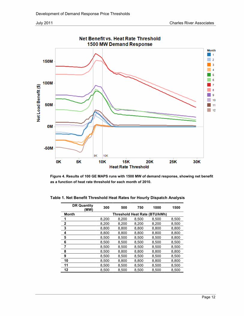
Figure 4 shows very similar results for the case in which 1500 MW of demand response is dispatched; results for the remaining scenarios are included in Appendix A. The net benefit threshold heat rates are translated into threshold LMPs using monthly average natural gas prices, and the results for all scenarios are shown in Table 1 and Table 2.

One of the principal findings of the hourly dispatch analysis was that the results were robust. That is, the net benefit threshold heat rate is relatively consistent across months, ranging from 8,200 to 8,800 BTU/kWh, and is relatively insensitive to demand response quantity. The corresponding LMPs vary more widely due to gas price volatility, and were found to be in the range of $33 to $69/MWh.


Page 11

Figure 3. Results of 100 GE MAPS runs with 500 MW of demand response, showing net benefit as a function of heat rate threshold for each month of 2010.


Page 12

Figure 4. Results of 100 GE MAPS runs with 1500 MW of demand response, showing net benefit as a function of heat rate threshold for each month of 2010.

Table 1. Net Benefit Threshold Heat Rates for Hourly Dispatch Analysis

DR Quantity (MW) 300 500 750 1000 1500

Month Threshold Heat Rate (BTU/kWh) 1 8,200 8,200 8,500 8,500 8,500 2 8,200 8,200 8,200 8,200 8,500 3 8,800 8,800 8,800 8,800 8,800 4 8,800 8,800 8,800 8,800 8,800 5 8,500 8,500 8,500 8,500 8,800 6 8,500 8,500 8,500 8,500 8,500 7 8,500 8,500 8,500 8,500 8,500 8 8,500 8,800 8,800 8,800 8,800 9 8,500 8,500 8,500 8,500 8,500 10 8,500 8,800 8,800 8,800 8,800 11 8,500 8,500 8,500 8,500 8,500 12 8,500 8,500 8,500 8,500 8,500


Page 13

Table 2. Net Benefit Threshold LMPs for Hourly Dispatch Analysis

DR Quantity (MW) 300 500 750 1000 1500

Month Threshold LMP ($/MWh) 1 $63.2 $63.2 $65.6 $65.6 $65.6 2 $53.9 $53.9 $53.9 $53.9 $55.9 3 $42.0 $42.0 $42.0 $42.0 $42.0 4 $39.1 $39.1 $39.1 $39.1 $39.1 5 $39.1 $39.1 $39.1 $39.1 $40.5 6 $44.7 $44.7 $44.7 $44.7 $44.7 7 $44.0 $44.0 $44.0 $44.0 $44.0 8 $40.8 $42.3 $42.3 $42.3 $42.3 9 $36.6 $36.6 $36.6 $36.6 $36.6 10 $32.8 $33.9 $33.9 $33.9 $33.9 11 $39.8 $39.8 $39.8 $39.8 $39.8 12 $69.2 $69.2 $69.2 $69.2 $69.2

5.2. Analysis of supply curves constructed from simulation inputs The net benefit test using supply curve analysis is outlined at a high level in Section 3. In this section the analysis and findings based on supply curves constructed from the simulation inputs are described in detail.

The generating plant input assumptions used in the hourly dispatch analysis, including capacity, generator heat rates, variable operating and maintenance costs, emissions costs, and fuel prices, were used to construct supply curves for each month.13 For the purposes of the supply curve analysis, the supply stack excluded imported power offerings and pumped storage generation, and ignored outages. Each unit was treated as a single block, using the full load heat rate, since one cannot easily capture the dynamics of startup cost, minimum generation levels and unit commitment in a simple supply stack. Despite these shortcomings, the simple supply stack represents a reasonable approximation to the supply curve averaged over each month.

From each of these raw supply curves, a smoothed supply function P(x) was formed, where x is the supply in MW, and P is the price, using non-linear regression on an appropriately sampled portion of the raw supply curve. It was found that a function of the following form, combining a cubic component with an exponential, yielded the best fit

(9)

where P(x) is the price in $/MWh as a function of x, the cumulative MW supply quantity, and e is the mathematical constant 2.718281828. The regression analysis yielded the best-fitting coefficients A through F. The exponential characteristic of the curve allows a reasonably good fit to the steep tail of the supply curve, where expensive and small peaking units

13 Supply curves differed from month to month inasmuch as fuel prices varied and due to seasonal changes in unit

capacity (summer and winter); generating plant input assumptions were based on publicly available data.


Page 14

dominate the supply stack, while the cubic characteristic allows a better fit to the broader, more gently rising portion of the curve going from large steam units to intermediate gas-fired combined cycle units. The lowest portion of the supply stack, consisting of low cost hydro, wind, nuclear, and some base load coal units, is not included in the fit, because it is clear from casual inspection that the supply stack has large elastic portions in this region of the supply curve. An example of the fit is shown in Figure 5 for June 2010, and similar figures for all months are included in Appendix A.

Once the coefficients were determined for each month, the resulting expressions represented smoothed supply curves with price P as a function of supply quantity x. The coefficients determined through this process are listed in Table 3.

A net benefit threshold for each month was then determined as the price on the curve above which an incremental quantity of supply (Δx) times the price (P(x)) is everywhere less than the associated incremental change in price, ΔP = P(x + Δx) – P(x), times the supply (x), as described in Section 3. For each curve, this point was found through an evaluation of the derivative at each point. The derivative of the function P in equation (9) is:

(10)

where the coefficients B through F have the same values determined by regression. Finally, a net benefit threshold price was determined as the price at the highest value of x on the smoothed supply curve for which the derivative of the curve (dP/dx) is equal to (P/x), i.e.,

Figure 5. Smooth curve fit to raw supply curve constructed from data used in the simulations for June 2010.

0

50

100

150

200

250

0 5000 10000 15000 20000 25000 30000 35000

Pric

e ($

/MW

h)

Cumulative Supply (MW)

ISO-NE Supply Stack - June 2010

Price

Fit

Inelastic

Elastic


Page 15

where the price elasticity of supply equals one.14 In Figure 5, the threshold can be seen at the point where the blue line through the origin is tangent to the fit curve. Note that the raw supply curve shown has many short flat portions above the threshold price (near $43.58 for June 2010, corresponding to a heat rate of 8,294 BTU/kWh).

We found that the threshold metric is sensitive to the details and granularity of the fitted curve choice: A smooth global fit will generally lead to lower threshold values than a more detailed fit with more local inflection points (bumps). The selected six-parameter expression yields a smooth curve with good overall fit to the supply curves examined, providing unambiguous thresholds at the highest elastic–to-inelastic transition points.

The resulting threshold LMPs were translated to implied heat rates using weighted average monthly natural gas prices. The threshold LMPs, ranging from $36 to $69/MWh, and corresponding heat rates, ranging from 8,250 to 9,520, are shown in Table 4. In general, they agree well with the results of the hourly dispatch analysis, indicating that the various factors not accounted for in the supply curve analysis, such as congestion, imports and exports, pumped storage, outages, startup costs, generator operating constraints, unit commitment, and load, are not significant determinants of net benefit thresholds in New England.

The thresholds were somewhat higher for one month, October (9,520, vs. 8,800 BTU/kWh from the hourly simulation). This can be explained in large part by low gas prices in that month, causing a larger relative contribution from variable operating and maintenance costs to the implied heat rate.

Table 3. Regression Coefficients for Supply Curve Used in Hourly Dispatch Analysis

Month A B C D E F 1 -62.70 208.98 -126.08 26.84 16.10 -47.59 2 -71.95 225.54 -140.49 29.64 22.71 -69.36 3 -11.51 -13.71 -1.33 -22.13 1.13 3.31 4 -54.00 -12.63 -19.31 -22.80 0.98 3.97 5 -191.74 437.35 -272.53 55.71 23.37 -68.59 6 -98.05 276.67 -178.97 37.89 86.42 -265.54 7 -132.30 333.77 -209.99 43.27 15.57 -45.62 8 -175.90 415.85 -262.38 54.10 27.69 -82.45 9 -187.60 420.72 -258.67 52.17 22.57 -67.40 10 -18.53 44.44 0.73 -11.22 1.84 0.26 11 5.90 26.07 2.49 -4.77 2.57 -2.93 12 -397.28 126.36 -151.94 23.95 0.34 5.77

14 The Commission in its Order specified that the test be done using a 1 MW interval. The formulation here is

equivalent, as the difference between the derivative dP/dx (the local slope we calculated for a very small interval of the smoothed supply curve) and Delta P / Delta X when Delta X =1 MW is trivial in the context of a 30,000 MW system.


Page 16

Table 4. Net Benefit Thresholds Determined through Analysis of Supply Curve Used in

Hourly Dispatch Analysis

Month Threshold Heat Rate

(BTU/kWh)* Threshold LMP ($/MWh)

1 8,830 $68.1 2 8,590 $56.5 3 8,800 $42.0 4 8,810 $39.1 5 8,480 $39.1 6 8,290 $43.6 7 8,250 $42.7 8 8,260 $39.7 9 8,680 $37.4 10 9,520 $36.7 11 8,960 $41.9 12 8,460 $68.9 * Rounded to nearest 10 BTU/kWh.

5.3. Analysis of generator offer supply curves

Having validated the unconstrained supply curve approach, we set out to apply it to actual generator offer data for 2010. This analysis was quite similar to that just described, except for assembly of the supply curves. We assembled monthly average supply stacks from daily real-time generator offers15 by first compiling each generator offer block (i.e., each price-quantity pair offered in the real-time energy market) for each day of the month and sorting the blocks in ascending order of price. The cumulative MW quantity at each price was calculated by summing the MWs in each block up to and including that price, and dividing by the number of days in the month. The result was an average supply stack for each month. For unbiased fitting, with equal weighting for each section of the supply curve, a sampled supply curve with uniform spacing on the x-axis (MW supply) was created from the raw data by finding the price at 25 MW intervals. We then fit smooth curves of the same cubic plus exponential function of equation (9), for the $25 to $300/MWh portion of interest for each month.16 Thresholds were then calculated using the derivatives of the curves, as in the analysis described above. Figure 6 shows the result for June 2010; Table 5 lists the regression coefficients, Table 6 lists the resulting net benefit thresholds, and Appendix A contains curves for the remaining 11 months. All of the regressions resulted in R2 statistics above 0.98.

Except in the winter months (December through February), the resulting threshold prices and corresponding implied heat rates shown in Table 6 are in the same general vicinity as — but somewhat lower than — those determined using the simulation input data.

15 These data are posted in masked form on the ISO-NE website at http://www.iso-

ne.com/markets/hstdata/mkt_offer_bid/rt_energy/2010/index.html.

16 Initial fits to full range showed we could ignore offers above $300; the smaller range allowed closer fits and more uniform results.

http://www.iso-ne.com/markets/hstdata/mkt_offer_bid/rt_energy/2010/index.html

http://www.iso-ne.com/markets/hstdata/mkt_offer_bid/rt_energy/2010/index.html


Page 17

Figure 6. Average supply stack constructed from generator offers, and corresponding curve fit and net benefit threshold, for June 2010.

Thresholds for January and December, however, are in the 5,600 BTU/kWh range ($43-$45/MWh). February’s threshold value is approximately 6,300 BTU/kWh ($41/MWh). In those months, relatively high natural gas prices reduce the contribution of variable operation and maintenance costs to the implied heat rate. As was the case in the analysis of supply curves derived from the data used in the hourly simulations, the heat rate implied by the October threshold is relatively high (nearly 9,000 BTU/kWh) due to the very low price of natural gas in that month.

Another observation worth noting is that in the winter months more than for others, the actual offer data (not the fitted curve) exhibit a region that is qualitatively almost straight and nearly tangent to a line to the origin, whereas raw offer data for other months show more distinctive threshold regions. As a result, the fit done slightly differently (e.g., with a different functional form) could have resulted in a threshold elsewhere along the straight region — the threshold is somewhat “fuzzy” in that sense. The January offer data, for example, form a nearly straight line from about $35 to $80/MWh (corresponding to 4,500 to 10,360 BTU/kWh at monthly average gas prices), and the December data are nearly straight from about $35 to $67/MWh (corresponding to 4,300 to 8,230 BTU/kWh). If the fit had been limited to offers from $30 - $90 (instead of from $25 to $300, used for consistency), it is likely that the resulting threshold would have been higher. Although we have not investigated the cause, it is possible that

Price ($/MWh)


Page 18

Table 5. Regression Coefficients for Supply Curves Based on Generator Offer Data for 2010

Month A B C D E F 1 57.97 -81.04 75.43 -12.93 5.25 -11.02 2 63.27 -82.53 63.20 -8.49 6.12 -14.13 3 30.52 5.99 -17.37 11.19 9.96 -26.09 4 -21.66 116.30 -89.99 25.05 11.12 -29.96 5 5.47 60.95 -56.45 19.80 8.56 -21.55 6 0.63 76.16 -64.98 21.38 8.75 -21.93 7 -5.61 97.15 -88.23 28.94 13.61 -35.86 8 -22.48 134.72 -116.38 35.30 13.97 -36.69 9 20.43 -5.64 -11.05 -3.69 1.46 1.90 10 -103.83 292.08 -216.34 54.93 16.80 -55.42 11 17.78 -4.80 -9.65 -1.90 1.36 1.97 12 26.83 0.32 6.52 4.82 11.17 -30.60

Table 6. Net Benefit Thresholds Determined through Analysis of Supply Curves based on Generator Offer Data for 2010

Month Threshold Heat Rate (BTU/kWh)* Threshold LMP ($/MWh)

1 5,640 $43.5 2 6,270 $41.2 3 7,630 $36.5 4 8,420 $37.4 5 7,910 $36.4 6 7,900 $41.5 7 7,490 $38.8 8 7,720 $37.1 9 7,920 $34.1 10 8,990 $34.7 11 7,730 $36.1 12 5,580 $45.4

* Rounded to nearest 10 BTU/kWh.

result is an artifact of the method (fitting to prices rather than implied heat rates), combined with intra-month volatility of gas and power prices. It is possible, therefore, that using weekly or daily fuel prices to normalize offers in months with volatile fuel prices prior to fitting would eliminate the problem. Likewise, translating the resulting threshold heat rates — in months when fuel prices are volatile — to weekly or even daily threshold prices using the corresponding fuel prices would yield threshold prices that would keep pace with changing fuel prices. The other months show a more distinctive threshold region (i.e., less fuzzy) in the raw and fitted curves.

5.4. Applying net benefit thresholds in practice Calculating and applying a net benefit threshold each month raises a number of practical considerations, discussed below.


Page 19

5.4.1. Fuel price volatility

One such consideration relates to the use of thresholds determined using historical offer data, given fuel price volatility. The Commission in its Order directed each ISO/RTO to determine the price threshold monthly,17 i.e., prior to the month in which it will be in effect, and therefore at a time when fuel prices for the effective month are not yet known. A potential result, however, is that a price threshold based on offers made during a time of low gas prices (or determined using average gas prices) would be too low for application in a period of high gas prices, potentially resulting in demand response that is not cost-effective being paid LMP.18 The Commission recognized that fixing the threshold for an entire month and in advance of the month “may result in instances both when demand response is not paid the LMP but would be cost-effective and when demand response is paid the LMP but is not cost-effective,” and stated that this outcome was acceptable given the difficulty of adopting a dynamic approach.19 The issue of fuel price volatility can be addressed to some extent by adjusting the price threshold to account for changes in the fuel price, e.g., by multiplying the threshold for the historical month by the ratio of the current or forecast fuel price index to the corresponding value of the index for the historical month. The efficacy of such adjustments will depend on how well the forecast or current value of the fuel price index approximates actual fuel prices, and how volatile fuel prices are within the month (which is primarily a consideration during winter months, as Figure 2 shows). Using more contemporaneous fuel prices (e.g., weekly or daily) to adjust price thresholds is an option that would have obvious advantages during periods with highly volatile fuel prices. These advantages would have to be weighed against any disadvantage resulting from less advance knowledge of threshold prices.20

In Section 5.3, we observed that thresholds determined using offer prices in months with high fuel price volatility may be less than robust. An alternative approach, fitting smooth supply curves to historical offer data normalized by intra-month fuel prices may yield more robust thresholds, and merits further investigation.

5.4.2. Variation in load from year to year

If loads are significantly lower, e.g., in operation than in the same month of the previous year used to determine the threshold, it is possible that the threshold would be so high that it would be reached less frequently. It is also possible that higher loads in the base year would result in thresholds being exceeded more frequently in the subsequent year. We have not analyzed historical data to determine how well a threshold determined in one year performs the following year, as that was beyond the scope of this study. Nevertheless, using the same

17 Order at ¶ 4.

18 The corollary result is demand response that is cost-effective being ineligible for payment.

19 Order at ¶ 80.

20 Such disadvantages could be offset somewhat by publishing threshold heat rates in advance, and fuel-adjusted threshold prices more frequently.


Page 20

month of the previous year to determine the threshold for the effective month will mitigate such considerations to some extent.

5.4.3. Frequency of clearing and impact on baseline accuracy

Demand response resources’ performance is commonly measured against baseline consumption levels. ISO-NE and others have found that when demand response resources clear for too many consecutive days, baseline accuracy can be adversely affected. To get a sense of how the number of consecutive business days with demand response would vary with threshold price levels, we analyzed 2010 real-time hourly prices to determine the maximum number of consecutive business days in a month in which a Load Zone exhibited implied heat rates at or above a range implied heat rate thresholds. The result is shown in Table 7, which shows the maximum (across Load Zones) number of consecutive business days in each month that demand response offers at the threshold price would have cleared.21 For some of the months, the net benefit thresholds estimated from 2010 generator offer data were met or exceeded for at least one hour on every business day (e.g., 20, 21, or 22 days), meaning that demand response would have cleared for consecutive business days spanning several consecutive months. It is our understanding at the time of this writing that ISO-NE will address this issue by modifying the way that baselines are refreshed, and is evaluating two alternative baseline refreshment methods.

A separate analysis commissioned by ISO-NE found that a two percent median relative error was an acceptable level of baseline bias, and also that up to 13 days can be excluded from the baseline calculation before the acceptable level of bias is exceeded (the “consecutive day criterion). One of the baseline refreshment methods under consideration involves adjusting a demand response asset’s baseline based on the relationships between its offer price, LMP, and a so-called Baseline Accuracy Price (“BAP”).

The BAP would be determined by identifying the highest hourly real-time LMP of any Load Zone for which the number of consecutive weekdays, excluding demand response holidays, with at least one hour at or above that LMP does not exceed the consecutive day criterion, and then adjusting that LMP to account for changes in fuel prices. The consecutive day criterion would be established in advance as the maximum number of days that a demand response asset’s meter data can be excluded from the computation of the asset’s baseline before baseline bias exceeds a two percent median relative error. The consecutive day criterion would be determined using data from September through December of the prior calendar year.

The implied heat rates that would meet a 13-day consecutive day criterion, based on an analysis of 2010 zonal real-time prices, can be found by examining the results shown in Table 7, and are summarized in Table 8, along with the corresponding LMPs.

21 The analysis was simplistic in the sense that it ignored the impact of demand response on price, and in turn the

impact on how often the demand response would clear. Consecutive day counts were reset at the start of each month, so that consecutive days at the end of one month and consecutive days at the beginning of the next would appear as two separate quantities in the table. The heat rate increments shown are the same as those used in the hourly dispatch analysis (i.e., 300 BTU/kWh).


Page 21

Table 7. Number of Consecutive Business Days with Prices at or Above the Implied

Heat Rate Threshold

Table 8. LMPs Meeting 13-day Consecutive Day Criterion for 2010

Month Heat Rate Meeting 13-Day

Criterion (BTU/kWh)*

LMP Meeting 13-day

Criterion ($/MWh)

1 9,100 $ 70.2 2 8,500 $ 55.9 3 9,100 $ 43.5 4 8,800 $ 39.1 5 12,100 $ 55.7 6 9,700 $ 51.0 7 13,000 $ 67.2 8 12,400 $ 59.5 9 14,200 $ 61.2 10 11,200 $ 43.2 11 11,200 $ 52.4 12 7,900 $ 64.3

* To nearest 300 BTU/kWh.


Page 22

6. Conclusion

The principal finding of the study was the validation of the supply curve approach with real-time generator offer data for use in determining threshold prices. It was found that a non-linear regression performed on a sampled portion of the unsmoothed supply curve could produce a smooth curve that closely approximates the unsmoothed curve and that net benefit thresholds determined using supply curves developed in this manner correspond closely to those determined using the much more sophisticated hourly dispatch analysis. Developing smooth supply curves using a non-linear regression of real-time generator offers, calculating net benefit thresholds based on those supply curves, and adjusting the thresholds using fuel price indices is a practical approach which ISO-NE can adopt for use in establishing demand response net benefit threshold prices in compliance with the Commission’s Order. A number of practical considerations for implementing the approach, including fuel price volatility, year-to-year variation in load, and baseline accuracy, are addressed in this report.


Page 23

Appendix A: Additional Figures


Page 24


Page 25

Supply Curve and Fit for January 2010, Using Simulation Supply Data

Supply Curve and Fit for February 2010, Using Simulation Supply Data


Page 26

Supply Curve and Fit for March 2010, Using Simulation Supply Data

Supply Curve and Fit for April 2010, Using Simulation Supply Data


Page 27

Supply Curve and Fit for May 2010, Using Simulation Supply Data

Supply Curve and Fit for June 2010, Using Simulation Supply Data


Page 28

Supply Curve and Fit for July 2010, Using Simulation Supply Data

Supply Curve and Fit for August 2010, Using Simulation Supply Data


Page 29

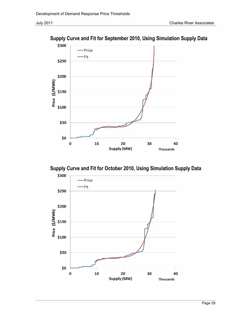
Supply Curve and Fit for September 2010, Using Simulation Supply Data

Supply Curve and Fit for October 2010, Using Simulation Supply Data


Page 30

Supply Curve and Fit for November 2010, Using Simulation Supply Data

Supply Curve and Fit for December 2010, Using Simulation Supply Data


Page 31


Page 32


Page 33


Page 34


Page 35


Page 36

development of demand response price thresholds...development of demand response price thresholds...

Documents