development of an optoelectronic holographic otoscope system for
TRANSCRIPT
Development of an optoelectronic holographic
otoscope system for characterization of sound-
induced displacements in tympanic membranes
A Thesis
submitted to the faculty of the
Worcester Polytechnic Institute
as a partial fulfillment of the requirements for the
Degree of Master of Science
in
Mechanical Engineering
by
_________________
Nesim Hulli
15 December 2008
Approved:
_______________________________
Prof. Cosme Furlong, Major Advisor
__________________________________________________
Prof. Ryszard J. Pryputniewicz, Member, Thesis Committee
____________________________________________
Prof. Glenn R. Gaudette, Member, Thesis Committee
__________________________________________________________________
Prof. John J. Rosowski, Mass. Eye & Ear Infirmary, Harvard-MIT Div. of Health
Sciences and Technology, Member, Thesis Committee
____________________________________________________________________
Dr. Maria del Socorro Hernández-Montes, CIO., MX., Member, Thesis Committee
_______________________________________________
Prof. Yiming Rong, Graduate Committee Representative

i
Copyright © 2008
By
NEST – NanoEngineering, Science, and Technology
CHSLT – Center for Holographic Studies and Laser micro-mechaTronics
Mechanical Engineering Department
Worcester Polytechnic Institute
Worcester, MA 01609-2280
All rights reserved

ii
ABSTRACT
The conventional methods for diagnosing pathological conditions of the
tympanic membrane (TM) and other abnormalities require measuring its motion while
responding to acoustic excitation. Current methodologies for characterizing the
motion of the TM are usually limited to either average acoustic estimates (admittance
or reflectance) or single-point mobility measurements, neither of which is sufficient to
characterize the detailed mechanical response of the TM to sound. Furthermore,
while acoustic and single-point measurements are useful for the diagnosis of some
middle ear disorders, they are not useful in others. Measurements of the motion of the
entire TM surface can provide more information than these other techniques and may
be superior for the diagnosis of pathology. In this Thesis, the development of an
optoelectronic holographic otoscope (OEHO) system for characterization of
nanometer scale motions in TMs is presented. The OEHO system can provide full-
field-of-view information of the sound-induced displacements of the entire surface of
the TM at video rates, allowing rapid quantitative analysis of the mechanical response
of normal or pathological TMs.
Preliminary measurements of TM motion in cadaveric animals helped
constrain the optical design parameters for the OEHO, including the following: image
contrast, resolution, depth of field (DOF), laser power, working distance between the
interferometer and TM, magnification, and field of view (FOV). Specialized imaging
software was used in selecting and synthesizing the various components. Several
prototypes were constructed and characterized. The present configuration has a
resolution of 57.0 line pairs/mm, DOF of 5 mm, FOV of 10 10 mm2, and a 473 nm
laser with illumination power of 15 mW.

iii
The OEHO system includes a computer controlled digital camera, a fiber optic
subsystem for transmission and modulation of laser light, and an optomechanical
system for illumination and observation of the TM. The OEHO system is capable of
operating in two modes. A „time-averaged‟ mode, processed at video rates, was used
to characterize the frequency dependence of TM displacements as tone frequency was
swept from 500 Hz to 25 kHz. A „double-exposure‟ mode was used at selected
frequencies to measure, in full-field-of-view, displacements of the TM surface with
nanometer resolution.
The OEHO system has been designed, fabricated, and evaluated, and is
currently being evaluated in a medical-research environment to address basic science
questions regarding TM function. Representative time-averaged holographic and
stroboscopic interferometry results in post-mortem and live samples are herein shown,
and the potential utilization discussed.

iv
This thesis is dedicated proudly to my family.
v
ACKNOWLEDGEMENTS
At this time, it is extremely important to extend my gratitude to a number of
individuals and organizations which have aided me and made it possible for me to
arrive at this moment with these results.
Most important, I‟m very grateful for all the support and friendship which
were offered to me by my advisor Professor Cosme Furlong, whom I shall never
forget. I thank Professor Ryszard Pryputniewicz for offering me the opportunity to
study interferometry and MEMS systems during my time at WPI. These professors
and my committee have demonstrated unwavering support during my Thesis research.
The Center for Holographic Studies and Laser micromechaTronics (CHSLT) in the
WPI Mechanical Engineering Department, for the use of both their facilities and
equipment, deserve much praise and recognition.
I wish to acknowledge the assistance of Professor John J. Rosowski and Dr
Jeffrey T. Cheng for their collaboration, advice and suggestions in my experimental
work. Funding and support from Dr. Saumil Merchant and his generous patients at
Massachusetts Eye and Ear Infirmary were extremely important in the project as well.
Accolades are also extended to Dr. Maria del Socorro Hernandez-Montes,
Ellery Harrington, and Haiyang Yang and from the CHSLT laboratories for their
enduring support and invaluable assistance.
Finally, I want to thank my dear family for their love and unending support
during my work over the past couple of years and more. Without them I would not
have been able to accomplish anything.

vi
TABLE OF CONTENTS
Copyright i
Abstract ii
Acknowledgements v
Table of contents vi
List of figures viii
List of tables xi
Nomenclature xii
Objective xvi
1. Introduction 1
2. Background 4
2.1. Anatomy of the ear 4
2.1.1. The tympanic membrane 6
2.1.2. Medical techniques and procedures 7
for diagnosis
3. Theory of interferometry 11
3.1. Fundamentals of interferometry 11
3.1.1. Electromagnetic wave propagation 12
3.1.2. The sensitivity vector, the fringe locus 14
function and the displacement vector
3.1.3. Double-exposure holography 17
3.1.4. Time-averaged holography 19
4. Implementation of optoelectronic holographic otoscope system 23
4.1. Fiber optic subsystem 24

vii
4.2. Otoscope head subsystem 25
5. Evaluation of the optoelectronic holographic otoscope system 39
5.1. Analytical results 41
5.2. Computational results 44
5.3. Results comparisons 46
6. Optoelectronic holographic otoscope system 49
in medical environment
6.1. Experimental results in tympanic membrane 50
7. Conclusions and future work 60
8. References 62
Appendix A. MATLAB code for line profile contrast calculation 69
Appendix B. Mathcad file for determining the sensitivity 72
vector for OEHO system

viii
LIST OF FIGURES
Fig. 2.1. Anatomy of the human ear: The cross section of human 5
ear showing divisions of the outer, middle, and inner ears
[Wikipedia, 2008].
Fig. 2.2. Middle ear ossicles: (a) chain of ossicles and their 5
ligaments, (b) the three bones: malleus (M) incus (I) and
stapes (S) [Csillag, 2005].
Fig. 2.3. Structure of the human tympanic membrane: (a) normal 6
tympanic membrane as seen through an otoscope
[Grundman et al., 2008], (b) schematic of a right tympanic
membrane [Sundberg, 2008].
Fig. 2.4. The tympanometer consists of a hand-held probe to be 8
inserted into the ear. The probe is composed of three tubes
containing a loudspeaker, a microphone and a pump
[Mikoklai et al., 2008].
Fig. 3.1. Electromagnetic wave propagation composed of 12
perpendicular electric and magnetic fields in the x-y plane.
Fig. 3.2. Illumination and observation geometry for holographic 14
interferometry: 𝑅𝑝 , 𝑅1, and 𝑅2 are the position vectors
whereas 𝑲1 and 𝑲2 are the illumination and the observation
vectors, respectively. 𝑲 is the sensitivity vector.
Fig. 4.1. Schematic of the OEHO system: TM is the sample 23
under investigation; OH is the otoscope head containing
an interferometer and imaging optics; FS is the fiber optic
subsystem containing a laser, beam splitting optics, and
laser-to-fiber components to provide an object beam (OB)
and reference beam (RB); OH and FS are controlled by the
image processing computer (IP). SS is the integrated sound
source, and MP is the microphone. FG is the frequency
generator which provides the timing input to the AOM driver
(AOMD).
ix
Fig. 4.2. Fiber optic subsystem: (a) schematic model depicting 24
the major components; (b) CAD model depicting the major
components; and (c) fabricated subsystem.
Fig. 4.3. Ray tracing using commercially available software. 26
So: Object to front principal point distance,
Si: Rear principal point to image distance, DOF: Depth of field.
Fig. 4.4. Diagram of the imaging system: (a) parameters of the 28
imaging system taken into account for the optical design.
FOV: Field of view, f: Focal length, ROI: Region of interest,
(b) target FOV of 10x10 mm2.
Fig. 4.5. MTF evaluated from OSLO software. 30
Fig. 4.6. Otoscope head subsystem: (a) schematic model depicting 33
the major components; (b) CAD models depicting the major
components; and (c) fabricated subsystem.
Fig. 4.7. USAF 1951 positive and negative target pattern 34
[Edmund Optics, Inc., 2006].
Fig. 4.8. Specification table for the USAF resolution target 35
[Edmund Optics, Inc., 2006].
Fig. 4.9. Recorded USAF 1951 negative glass target with group 5 36
outlined for containing the smallest resolvable element set
[Edmund Optics, Inc., 2006].
Fig. 4.10. Line profile contrast calculation method (a) image of G4E2 37
showing a line profile, (b) line intensity profile and contrast
calculation.
Fig. 5.1. A coated copper foil mounted on to the piezoelectric shaker. 39
Fig. 5.2. Time-averaged interferograms of a test copper sample. 41
Fig. 5.3. First mode of vibration obtained with MathCAD 44
[Dwyer et al., 2008].
Fig. 5.4. Finite element method results for natural frequencies of a 45
test copper sample [Dwyer et al., 2008].
Fig. 6.1. OEHO system installation: (a) OEHO system at MEEI; 49
(b) otoscope head subsystem testing post mortem

x
human temporal bone at MEEI; and (c) otoscope head
subsystem testing post mortem chinchilla at MEEI.
Fig. 6.2. Time-averaged holograms measured in cadaveric humans, 51
in cadaveric chinchilla, in live chinchilla, and in cadaveric
cat. The schematic on the top row shows the area of the
TM in gray, location of the malleus, the umbo and the probe tube.
Fig. 6.3. Synchronization of the illumination with the object excitation. 52
Fig. 6.4. Full-field-of-view stroboscopic holography measurements 54
in human temporal bone at 500 Hz, showing a peak-to-peak
surface out of plane displacement on the order of 90nm:
(a) unwrapped phase (2D plot); and (b) 3D plot.
Fig. 6.5. Full-field-of-view stroboscopic holography measurements 55
in human temporal bone at 800 Hz, showing a peak-to-peak
surface out of plane displacement on the order of 120nm:
(a) unwrapped phase (2D plot); and (b) 3D plot.
Fig. 6.6. Full-field-of-view stroboscopic holography measurements 56
in human temporal bone at 4 kHz, showing a peak-to-peak
surface out of plane displacement on the order of 190nm:
(a) unwrapped phase (2D plot); and (b) 3D plot.
Fig. 6.7. Full-field-of-view stroboscopic holography measurements 57
in human temporal bone at 12 kHz, showing a peak-to-peak
surface out of plane displacement on the order of 150nm:
(a) unwrapped phase (2D plot); and (b) 3D plot.
Fig. 6.8. Full-field-of-view stroboscopic holography measurements 58
in human temporal bone at 15 kHz, showing a peak-to-peak
surface out of plane displacement on the order of 210nm:
(a) unwrapped phase (2D plot); and (b) 3D plot.
Fig. 6.9. Full-field-of-view stroboscopic holography measurements 59
in human temporal bone at 20 kHz, showing a peak-to-peak
surface out of plane displacement on the order of 60nm:
(a) unwrapped phase (2D plot); and (b) 3D plot.
xi
LIST OF TABLES
Table 4.1. Lenses tested. 28
Table 4.2. Working distance constraints. 38
Table 5.1. Membrane test data. 40
Table 5.2. First six mode shapes and frequencies provided with 46
ACES methodology [Dwyer et al., 2008].
Table 5.3. Experimental result percent error [Dwyer et al., 2008]. 48

xii
NOMENCLATURE
magnitude
(x, y) coordinates
∆𝜙 random phase difference between 𝜙𝑜 and 𝜙𝑟
Δ𝜃 known phase step introduced between the frames
Δ𝑡 exposure of the camera
𝜖 electric permittivity of the medium
angle of incidence
𝜃𝑛 phase step
𝜆 laser wavelength
𝑣 wave propagation velocity
∅ relative phase between two waves
𝜙𝑜 randomly varying phase of the object beam
𝜙𝑟 phase of the reference beam
𝜔 circular frequency
Ω fringe locus function
Ωt time varying fringe locus function
f focal length
𝑘 wave number, 2𝜋
𝜆
𝐤 elastic modulus of the plate
ll line length
𝑚 the rank of the root
𝑛 the order of the root
n fringe order number
𝑛(𝑥, 𝑦) fringe order number at known (x, y)
psCCD pixel size of the CCD
𝑡 time

xiii
𝐴1, 𝐴2 vector amplitudes
𝐴𝑛 , 𝐵𝑛 , 𝐶𝑛 , 𝐷𝑛 the coefficients used to determine the mode shapes
𝐴𝑜 amplitude of an object beam
𝐴𝑟 amplitude of a reference beam
𝐵 magnetic field
𝐵𝑟 beam ratio
C contrast
𝐷 flexural rigidity of the plate
Da aperture diameter
Dl lens diameter
DOF depth of field
𝐸 electric field
𝐸1, 𝐸2 electric field vectors
F/# f number
𝐹𝑜 , 𝐹𝑟 complex light fields
FOV field of view
𝐼 intensity
Imax the maximum interferogram intensity
Imin the minimum interferogram intensity
𝐼𝑛 phase stepped intensity
𝐼𝑛 ′ intensity of the deformed object
𝐼𝑜 intensity of the object beam
𝐼𝑟 intensity of the reference beam
𝐼𝑡𝑛 𝑥, 𝑦 intensity distribution of the 𝑛-th frame where 𝑛 = 4
𝐽𝑛 Bessel functions of the first kind
𝐽𝑜 zero order Bessel function of the first kind
𝑲 sensitivity vector

xiv
𝑲1 illumination vector
𝐾1𝑥 , 𝐾1𝑦 , 𝐾1𝑧 Cartesian components of the illumination vector
𝑲2 observation vector
𝐾2𝑥 , 𝐾2𝑦 , 𝐾2𝑧 Cartesian components of the observation vector
𝐾𝑛 the modified Bessel functions of the second kind
𝑳 displacement vector
𝑀 characteristic function
MAG magnification
NA numerical aperture
ROI region of interest
𝑅𝑝 , 𝑅1, 𝑅2, 𝑅𝑛 position vectors where 𝑛 = 1,2, 𝐏
𝑅𝑥 , 𝑅𝑦 , 𝑅𝑧 Cartesian components of the position vectors
Si image distance
So object distance
𝑊 deformation of the plate
𝑌𝑛 Bessel functions of the second kind
𝑍𝑛 the modified Bessel functions of the second kind
ACES analytical, computational, and experimental solutions
AOM acousto-optic modulator
AOMD acousto-optic modulator driver
BS beam splitter
BSI imaging beam splitter
CCD charge-coupled device
FA laser-to-fiber coupler assemblies
FEM finite element method
FG frequency generator
FS fiber optic subsystem
xv
I incus
IS imaging system
IS illumination source
IP image processing computer
LD laser
LDV laser doppler vibrometry
M mirror
M malleus
MEMS microelectromechanical systems
MP microphone
MPM mirror mounted onto piezoelectric modulator
MTF modulation transfer function
O observation source
OB object beam
OEHO optoelectronic holographic otoscope
OH otoscope head
P random point on the object
Pi principal inertia of the plate
RB reference beam
Ri rotary inertia of the plate
S speculum
S stapes
SLV scanning laser vibrometer
SS sound source
TM tympanic membrane
xvi
OBJECTIVE
The objective of this Thesis is the development of a compact, full-field-of-
view optoelectronic, high-speed measurement system for otology applications. The
measurement system is based on an optoelectronic holographic otoscope (OEHO)
which enables measurements of shape and deformations of nanometer scale resolution
in tympanic membranes (TMs). This Thesis will demonstrate the effectiveness of the
OEHO; validate the optomechanical design and the measurements provided by the
OEHO, and present new data for different species.

1
1. INTRODUCTION
Recent advances in medical technology have given medical professionals
increasingly accurate tools. In all aspects of the medical fields, sophisticated
equipment is being used for everything from making diagnoses to performing
surgeries. Currently, knowledge of both the functionality of the middle ear and
related hearing conditions is expanding as a result of these new technologies. In
particular, the tympanic membrane (TM) is being examined more quantitatively than
ever before.
The TM, which plays an important role in the transmission of sound into the
cochlea, is a tissue separating the external ear canal from the middle ear cavity
[Rosowski, 1996]. Experimental measurements and theoretical analysis have been
done to study the structure [Lim, 1970, 1995], mechanical properties [Funnel and
Laszlo, 1978; Fay et al., 2005] and acoustic function [Tonndorf and Khanna, 1970;
Rosowski et al., 1986] of the TM.
The efficiency of sound coupling through the TM can be hindered by changes
to the TM through trauma or middle-ear diseases. By measuring the deformation of
the TM with various acoustic stimuli, the degree of hearing loss can be determined.
Most present day middle ear diagnostic procedures are based on acoustic
measurements that sense the mobility of the entire TM, e.g., multi or single frequency
tympanometry [Shanks et al., 1988; Margolis et al., 1999], ear canal reflectance or
power absorption [Keefe et al., 1993; Feeney et al., 2003; Allen et al., 2005], and
static pressure induced variations in sound pressure [Wada et al., 1989]. However,
single-point laser vibrometer measurements of the mobility of the umbo in the TM

2
have also been used as diagnostic aids in the clinic [Huber et al., 2001; Whittemore et
al., 2004; Rosowski et al., 2008].
All of these clinic measurements have weaknesses. The acoustic
measurements depend on the sound pressure at the TM and represent the average
mobility of the entire TM. The single-point laser vibrometry measurements are much
more localized, which may lead to a superior ability to distinguish ossicular disorders
[Rosowski et al., 2008], but are relatively insensitive to TM disorders at locations
other than the umbo. Full-field-of-view measurements of the TM mobility may be
superior to either of the present techniques in that they will quantify the motion of the
entire surface of the TM. Optoelectronic holography, which has been successfully
tested in many applications and environments, [Pryputniewicz et al., 2002] in this
regard has shown the capability to provide the desired information on the state of the
tympanic membrane.
Holographic methodologies have been used in the past to enable full-field-of-
view measurements of the vibrating patterns of the surface of the TMs, but there are
only a few holographic studies, which describe the motion of the entire mammalian
TM within a limited frequency range (0.1 ~ 8 kHz) [Wada et al., 2002; Khanna and
Tonndorf, 1972; Tonndorf and Khanna, 1971].
Currently, the most detailed description of the motion of the TM comes from
time-averaged holograms measured in animals [Khanna and Tonndorf, 1972] and
human cadavers [Tonndorf and Khanna, 1972]. These data provide good qualitative
descriptions of the magnitude of sound-induced motions of the TM surface.
However, the published data using these techniques are few. Therefore, some
fundamental questions of TM functions have not been answered.

3
In this Thesis, the sound-induced motion of the TM surface in postmortem
preparations from three mammalian species: cat, chinchilla (including one live
chinchilla) and human cadavers, were measured using an optoelectronic holographic
otoscope (OEHO) system.
The OEHO system, which is designed for fields-of-view on the order of 10
mm in diameter, uses a solid state laser (wavelength 𝜆 = 473 nm) and is operated in
two modes. The „time-averaged‟ holography mode is used for rapid identification of
resonant frequencies and corresponding mode shapes of vibration of samples [Furlong
and Pryputniewicz, 1996]. The „double-exposure‟ mode is used for determination of
the magnitude and phase of displacements over the entire TM surface with nanometer
resolution [Furlong et al., 2007].
As with the development of any system, at some point it becomes necessary to
demonstrate its integrity. An understood geometry with characteristics or qualities
that were predictable was necessary to compare and draw conclusions with the
experimental results that could be derived. Because tympanic membrane geometry is
complex, the performance of the system was evaluated with a simplified circular plate
employing finite element and analytical methods, as well as experimental data.
Additionally, described herein are the advances in the design, fabrication,
characterization, and use of a compact, stable OEHO system currently in use in
medical research environments.

4
2. BACKGROUND
2.1. Anatomy of the ear
Anatomically, the mammalian ear can be divided into three functional parts as
shown in Fig. 2.1: the outer (external) ear, the middle ear and the inner ear. The
external ear which consists of auricle or pinna (the visible part of the ear) and the
external auditory canal collects sound waves and transmits them to the middle ear.
The middle ear is a space filled with air that encapsulates the three middle ear
bones (ossicles) and the middle ear muscles as presented in Fig. 2.2. The first bone,
the hammer (malleus), is connected to the anvil (incus), which in turn is connected to
the stirrup (stapes). The middle ear is attached to the back of the nose (nasopharynx)
by the Eustachian tube. In the same way that the outer ear is an apparatus of hearing,
so is the middle ear. Namely, the sound energy coming from the outer ear causes the
TM to vibrate. The tympanic membrane transforms acoustic energy to mechanical
energy in the form of ossicular motion. The stapes converts mechanical energy to
acoustic energy within the inner ear.
The inner ear contains the semicircular canals, the vestibule for balance, and
the cochlea for hearing. The inner ear is where “hearing” actually takes place.
Signals sent from outside are received by the inner ear, which then interacts
neurologically with the brain via the vibration of microscopic „hairs‟ (the stereocilia)
with varied lengths that are attached to sensory cells. The „hair cells‟ are arranged in
an orderly fashion along the length of the auditory inner ear, where those that respond
to lower frequencies are farther from the stapes. This tonotopic mapping allows the
coding of sound frequency and the perception of pitch.

5
Fig. 2.1. Anatomy of the human ear: The cross section of human ear showing
divisions of the outer, middle, and inner ears [Wikipedia, 2008].
(a) (b)
Fig. 2.2. Middle ear ossicles: (a) chain of ossicles and their ligaments, (b)
the three bones: malleus (M) incus (I) and stapes (S) [Csillag, 2005].

6
2.1.1. The tympanic membrane
The tympanic membrane is a semi-transparent, thin, cone shaped membrane
which is the boundary between the outer and middle ears, as presented in Fig. 2.3.
(a) (b)
Fig. 2.3. Structure of the human tympanic membrane: (a) normal tympanic
membrane as seen through an otoscope [Grundman et al., 2008],
(b) schematic of a right tympanic membrane [Sundberg, 2008].
The TM is composed, structurally, of three layers. The lateral (or outside)
layer is a skin-like epidermis, the medial (or inside) layer is mucosal lining much like
the lining of the mouth and nose. In between is a fiber rich connective layer, called
the lamina propria [Sanna et al., 2003]. The diameter of the TM is 5-10 mm, and the
depth of cone is about 1.5mm [Dirckx and Decraemer, 2000]. The exterior edge of
the TM, named the annulus, or the annular ring, consists of a fibrous and cartilaginous
tissue that is both thicker and stiffer than the rest of the membrane [Sundberg, 2008].
The TM is between 55 and 140 micrometers thick [Kuypers et al., 2006]; it is thinnest
7
in the central parts of the posterosuperior quadrant and thickest in the vicinity of the
inferior part of the annulus. The triangular extension at the superior part of the TM is
the flexible pars flaccida. The flaccida is about 10% of the area of the TM, and
moves independently from the balance of the TM area, the pars tensa, that is tightly
coupled to the ossicular chain [Sundberg, 2008].
Since TM has unique anatomical and physical features that are ideally suited
for the sound transmission in varying frequency ranges, it plays an important role in
the diagnosis of middle ear disorders.
2.1.2. Medical techniques and procedures for diagnosis
To diagnose any unhealthy conditions of the middle ear, there are a limited
number of different methods practiced. Developed by clinicians, tympanometry,
Fig. 2.4, is a measure of the mobility of the TM and middle ear and depends on the
status of the TM, the middle-ear air space and the ossicular chain [Schubert, 1980;
Mikoklai et al., 2008]. Tympanometry is routinely used to help detect the presence of
fluid in the middle-ear and TM perforations, but is less useful in the diagnosis of
ossicular disorders.
Graphical representation of the relationship between air pressure in the external
canal to the impedance of the tympanic membrane and the middle ear system can be
supplied by tympanometry [Mikoklai et al., 2008]. In effect, impedance is inversely
related to the mobility of the tympanic membrane; this is in actuality what physicians
are testing when they determine the health of a patient‟s tympanic membrane
[Schubert, 1980]. The physics of transmitting sound is much like what happens when

8
a drum is struck: part of the sound is reflected while the other part is absorbed by the
instrument itself.
Likewise, when the tympanic membrane is hit by a sound, some of the sound
waves are absorbed and sent to the inner ear by the ossicles, while the remaining part
of the sound is reflected back.
Fig. 2.4. The tympanometer consists of a hand-held probe to be inserted into
the ear. The probe is composed of three tubes containing a loudspeaker, a
microphone, and a pump [Mikoklai et al., 2008].
Abnormal TM mobility is an indication of a „conductive‟ hearing loss: a
problem with how sound is conducted to the inner ear sensory mechanism. A
„sensory‟ or „neural‟ hearing loss describes a pathology associated with the
conversion of sound energy into electrical energy within the hair cells and the
conduction of these electrical sensory signals to the brain. The sensory or neural
hearing losses are differentiated from conductive pathologies via the use of
9
„bone-conduction‟ hearing test. In bone-conduction testing, sound is presented to the
inner ear via a mechanical vibrator placed firmly on the skull. The bone-conducted
sound is thought to bypass the middle ear and stimulate the inner-ear directly. A
person with a loss of sensitivity to air-conducted sound and normal sensitivity to
bone-conducted sound is thought to have a „conductive‟ hearing loss related to either
middle or external-ear pathology.
Physicians induce different pressures in the ear canal and take measurements
with relation to available volumes (fluid in the cochlea) [Schubert, 1980]. If the
recorded volumes are found to be different from that of the normal ear, then it is very
likely that there is a problem in the middle ear [Schubert, 1980]. The type of pattern
detected can also help to determine what type of middle ear condition the patient has,
enabling physicians to begin determining the method of treatment [Katz, 1994]. This
type of analysis, together with the use of an otoscope, provides the information
necessary to make proper diagnoses of specific ear ailments [Katz, 1994]. This type
of testing requires various kinds of expertise and a large commitment of time.
A non contact system that uses Laser Doppler Vibrometers (LDV) to map
tympanic response is the newest experimental method to test the tympanic membrane.
First, the device ascertains and reports the velocity of surfaces in a system and then
extracts relevant data for use by audiologists [Rosowski et al., 2008; Castellini et al.,
2006]. These measurements have been demonstrated to be sensitive to several
middle-ear pathologies including TM perforations and ossicular fixations and
interruptions. When applied to a sample, the LDV supplies point-by-point
information [Rosowski et al., 2008]. LDV can be used to measure vibrations in order
10
to collect multiple data points at a time and receive a magnified “field-of-view” of
their data.
Used in combination with a Scanning Laser Vibrometer (SLV) to collect data
from multiple points on a sample simultaneously, points within a minute area for
example, to provide the whole image of the sample‟s response [Castellini, et al.,
1998].
There are other methods that have the capability to provide data on the TM
response to be used for further analysis. Holographic interferometry, as a hybrid
optical testing method, is helpful in analysis of sample deformation in full-field-of-
view [Furlong and Pryputniewicz, 1998; Furlong et al., 2002; Furlong et al., 2008;
Hulli et al., 2007; Hernández-Montes et al., 2008]. It must be remembered that single
point measurements are not sufficient to characterize the motion of the entire TM.
Special analysis equipment is required for full-field-of-view measurement
methodologies of nanometer resolution if comprehensive data about the tympanic
membrane is to be provided.
Optoelectronic holographic interferometry is one of the current areas of laser-
related research capable of providing physicians with desired information on the
condition of tympanic membranes. Theoretical aspects of interferometry will be
addressed in the next section.

11
3. THEORY OF INTERFEROMETRY
3.1. Fundamentals of interferometry
Interferometry is a non-contact metrology technique that is capable of
measuring absolute shape and deformation based on the interference of the light. Two
waves of identical origin create interference patterns at the observer (bright and dark
fringes) by following optical paths of different lengths, a result of the changing
distance to the object‟s surface. Each fringe corresponds to a distance change equal to
one half the wavelength of the light [Kreis, 2005].
However, the coherence and monochromativity of light sources used in
standard interferometers prior to 1960 were poor [Pryputniewicz, 1996]. As a result,
classical interferometry was limited to measurements of small path-length differences
of optically polished and reflecting flat surfaces [Pryputniewicz, 1996].
In the early 1960‟s, with the advent of light amplification by stimulated
emission of radiation (laser), holography permitted interferometry to overcome this
shortcoming without any alterations of the fundamental principles. The technique,
based on the ability of a hologram to record the phase and amplitude of any wave,
was developed by Stetson and Powell, and is known as holographic interferometry
[Holophile, Inc., 2008].
Holographic interferometry revolutionized nondestructive evaluation
techniques and went on to become one of the major achievements in optics at the turn
of the last century [Kreis, 2005]. Holographic interferometry demands that the same
medium be used to record an object from different positions. The interference of the
reconstruction from multiple exposures of the object is created by the diffraction
patterns; these produce fringe patterns on the reconstructed surface, which indicate the

12
movement of the object during the test period. The interferometric procedure has a
measurement range that depends on the number of fringes that can be resolved by the
CCD camera. Using a high resolution CCD camera, and a highly reflective object,
out-of-plane measurements can have a range of approximately 0 to 50 µm, with a
resolution on the order of a few nanometers or better [Kreis, 2005].
The basis of holographic interferometry, that is, the theories of wave
propagation and interference, can be explained vis a vis holographic interferometry.
It is vital that the basic element of electromagnetic wave propagation and interference
be understood before presenting the theoretical aspects of hologram interferometry.
This will be addressed now.
3.1.1. Electromagnetic wave propagation
The study of the interaction of light waves as they intersect one another in
some medium comprises the foundation of optical interferometry [Hecht, 1989].
Light is an electromagnetic wave which can be explained in terms of an electric field
component (𝐸) and a magnetic field component (𝐵). These two fields are
perpendicular to each other, and the composed wave of 𝐸 and 𝐵 travels in the
direction of 𝐸 × 𝐵 as it can be seen in Fig. 3.1
Fig. 3.1. Electromagnetic wave propagation composed of perpendicular electric and
magnetic fields in the x-y plane.
13
In holography, the devices used to record images are only sensitive to the
electric field component. In fact, it is the time-averaged intensity of the electric field
squared which is detected [Robinson and Reid, 1993; Vest, 1979].
From the Maxwell equations we get the intensity as
𝐼 = 𝜖𝑣 𝐸2 , (3.1)
where I is the intensity, 𝜖 is the electric permittivity of the medium in which the wave
propagates at velocity 𝑣 and 𝐸2is the time-average of the electric field squared. Thus
we only use proportionality between the square of the electric field and the intensity
𝐼 ∝ 𝐸2 . (3.2)
Interference is the combination of two or more coherent light waves emitted
by the same source, which differ in the direction to form a resultant wave. Light
waves are subject to the superposition principle. For example if two waves overlap
the resulting fields is the vector sum of the two original fields,
𝐸 = 𝐸1 + 𝐸2 . (3.3)
The corresponding intensity due to these fields is then
𝐼 = 𝐸2 = 𝐸12 + 𝐸2
2 + 2 ∙ 𝐸1 ⋅ 𝐸2 . (3.4)
For simplicity let‟s assume that both waves are linearly polarized in the same
direction. The equations for the electric field vectors 𝐸1 and 𝐸2 can be written
respectively as,
𝐸1 = 𝐴1 cos 𝜔𝑡 − 𝑘1 ∙ 𝑟 , (3.5)
and
𝐸2 = 𝐴2 cos 𝜔𝑡 − 𝑘2 ∙ 𝑟 + ∅ (3.6)
14
where 𝐴1 and 𝐴2 are the vector amplitudes, 𝜔 is its circular carrier frequency, 𝑡 is the
time, k is the wave number (2∙𝜋
𝜆), and ∅ is the relative phase between two waves.
Finally, combining equations 3.4, 3.5, and 3.6 the intensity of two overlapping electric
fields can be found to be
𝐼 = 𝐴12 + 𝐴2
2 + 2𝐴1𝐴2 cos 𝑘2 ∙ 𝑟 − 𝑘1 ∙ 𝑟 − ∅ . (3.7)
3.1.2. The sensitivity vector, the fringe-locus function, and the displacement
vector
In addition to the description of the light fields, there are also three other
quantities: the sensitivity vector, the displacement vector and the fringe locus
function, which are important due to the quantitative analysis of holographic
interferometry [Pryputniewicz, 1994-a, 1996; Pryputniewicz and Stetson, 1980]. The
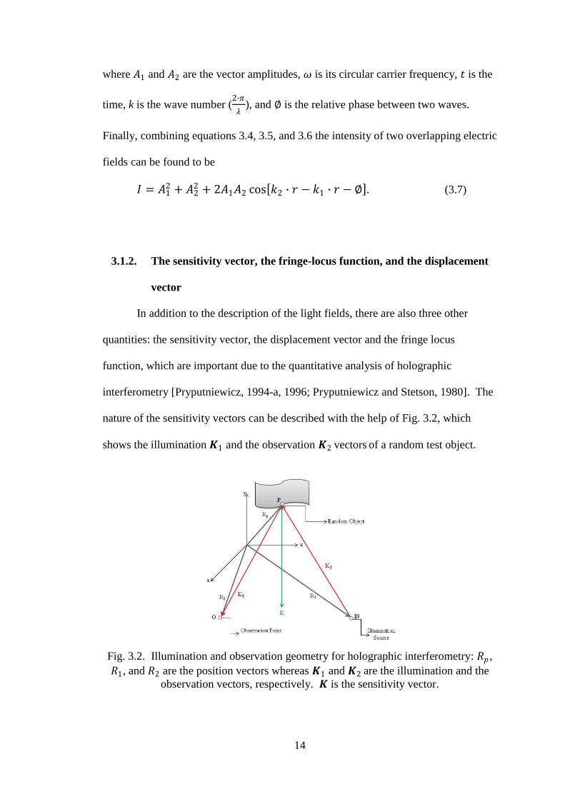
nature of the sensitivity vectors can be described with the help of Fig. 3.2, which
shows the illumination 𝑲1 and the observation 𝑲2 vectors of a random test object.
Fig. 3.2. Illumination and observation geometry for holographic interferometry: 𝑅𝑝 ,
𝑅1, and 𝑅2 are the position vectors whereas 𝑲1 and 𝑲2 are the illumination and the
observation vectors, respectively. 𝑲 is the sensitivity vector.

15
In Fig 3.2, IS illustrates the illumination source, e.g. laser, O is the
observation point, e.g. camera, detector, or simply an eye, and P is an randomly
selected point on the sample, where 𝑅1, 𝑅2 and 𝑅𝑝 are the position vectors which
describe the spatial coordinates of these points.
These position vectors are described as
𝑅𝑛 = 𝑅𝑛𝑥 𝑖 + 𝑅𝑛𝑦 𝑗 + 𝑅𝑛𝑧 𝑘 𝑛 = 1,2, 𝐏 (3.8)
where 𝑅𝑥 , 𝑅𝑦 , and 𝑅𝑧 are the Cartesian components of these vectors.
The illumination and observation vectors 𝑲1 and 𝑲2 can be written
respectively in Cartesian components as,
𝑲1 = 𝐾1𝑥 𝑖 + 𝐾1𝑦 𝑗 + 𝐾1𝑧𝑘 (3.9)
and
𝑲2 = 𝐾2𝑥 𝑖 + 𝐾2𝑦 𝑗 + 𝐾2𝑧𝑘. (3.10)
Correspondingly they can be expressed in terms of the position vectors depicted in
Eq. 3.8 as
𝑲1 = 𝑘𝑅𝑝−𝑅1
𝑅𝑝−𝑅1 , (3.11)
and
𝑲2 = 𝑘𝑅2−𝑅𝑝
𝑅2−𝑅𝑝 . (3.12)
In the above equations indicates a magnitude of the quantity between the
vertical bars, 𝑘 is the magnitude of the propagation vectors 𝑲1 and 𝑲2, and it is
related to the wavelength (𝜆) of the laser light
𝑲1 = 𝑲2 = 𝑘 =2𝜋
𝜆. (3.13)
16
Based on the results from Eqs 3.11 and 3.12, the sensitivity vector 𝑲, which
specifies the direction of deformation to which a holographic setup will be most
sensitive, can be calculated (Appendix B) as the difference between the observation
vector 𝑲1, and the illumination vector 𝑲2,
𝑲 = 𝑲2 − 𝑲1. (3.14)
The methods of holographic interferometry allow measurement range of
object displacements from a hundredth to several hundreds of a wavelength [Kreis,
2005; Vest, 1979].
As an object deforms or is displaced during the recording of a hologram, the
optical path length of the light reflected off the object changes. These results in phase
differences are recorded in the form of fringes. These fringes are described by a
fringe-locus function (Ω) constant values of which define fringe loci on the object‟s
surface. The fringe-locus function relates directly to the fringe orders (𝒏)
Ω = 2𝜋𝒏. (3.15)
Additionally, the fringe-locus function can be related to the scalar product of the
sensitivity vector 𝑲 with the displacement vector 𝑳 as
Ω = 𝑲 ∙ 𝑳. (3.16)
In this Thesis, the methods of double-exposure holography and time-averaged
holography (discussed in sections 3.1.3 and 3.1.4, respectively) were used to
investigate vibrations of the TMs.

17
3.1.3. Double-exposure holography
In optoelectronic holography [Pryputniewicz, 1996; Furlong and
Pryputniewicz, 1998; Hulli et al., 2007] information (mechanical deformations or
displacements) in double-exposure investigations is related to the optical path change
which can be extracted from the interference pattern of object and reference beams
having complex light fields 𝐹𝑜 and 𝐹𝑟 respectively as
𝐹𝑜 = 𝐴𝑜𝑒𝑥𝑝 𝑖 𝜙𝑜 + 𝜃𝑛 , (3.17)
and
𝐹𝑟 = 𝐴𝑟𝑒𝑥𝑝 𝑖 𝜙𝑟 . (3.18)
After the beam splitter and considering phase stepping, intensity 𝐼𝑛 of the
combined wavefronts as recorded by the n-th video frame can be described by
𝐼𝑛 = 𝐹𝑜 + 𝐹𝑟 𝐹𝑜 + 𝐹𝑟 ∗,
= 𝐴𝑂 𝑒𝑥𝑝 𝑗 𝜙𝑜 + 𝜃𝑛 + 𝐴𝑟𝑒𝑥𝑝 𝑗𝜙𝑟 𝐴𝑂
𝑒𝑥𝑝 −𝑗 𝜙𝑜 + 𝜃𝑛 +
𝐴𝑟𝑒𝑥𝑝 −𝑗𝜙𝑟 ,
= 𝐴𝑜 2 + 𝐴𝑟
2 + 2𝐴𝑜𝐴𝑟𝑐𝑜𝑠 𝜙𝑜 − 𝜙𝑟 + Δ𝜃𝑛 , (3.19)
where 𝐴𝑜 and 𝐴𝑟 are the amplitudes of the object and reference beams, 𝜙𝑜 is the
randomly varying phase of the object beam, 𝜙𝑟 is the phase of the reference beam,
and Δ𝜃 is the known phase step introduced between the frames. To facilitate double-
exposure investigations, the argument of the periodic term of Eq. 3.19 is modified to
include the phase change due to deformations of the object of interest subjected to
specific loading and boundary conditions. This phase change is characterized by the
fringe locus function Ω as

18
Ω 𝑥, 𝑦 = 2𝜋𝑛 𝑥, 𝑦 = 𝑲2 𝑥, 𝑦 − 𝑲1 𝑥, 𝑦 ∙ 𝑳 𝑥, 𝑦
= 𝑲 𝑥, 𝑦 ∙ 𝑳 𝑥, 𝑦 , (3.20)
where 𝒏 𝑥, 𝑦 is the interferometric fringe order at the known 𝑥, 𝑦 coordinates, 𝑲 is
the sensitivity vector, and 𝑳 is the displacement vector. Therefore, the intensity from
a deformed object can be described by the intensity distribution (𝐼𝑛′).
𝐼𝑛′ = 𝐼𝑜 + 𝐼𝑟 + 2𝐴𝑜𝐴𝑟𝑐𝑜𝑠 ∆𝜙 + Ω + Δ𝜃𝑛 , (3.21)
where ∆𝜙 is the random phase difference between two fields; ∆𝜙 = 𝜙0 − 𝜙𝑟 , and 𝐼0
and 𝐼𝑟 represent the intensities of the object and reference beams, respectively. In Eq.
3.21, 𝐼0 is assumed to remain constant and the 𝑥, 𝑦 arguments are omitted for
clarity. Since it is Ω which carries information pertaining to mechanical
displacements and/or deformations, the optoelectronic holography‟s video processing
algorithm eliminates ∆𝜙 from the argument of the periodic function of the intensity
distributions given in Eqs 3.19 and 3.21 by sequentially recording four frames with an
introduction of a 90° phase shift between each frame. By solving the two sets of four
simultaneous equations yields an image which is intensity modulated by a periodic
function with Ω as the argument.
The optoelectronic holography operates in either display or data mode
[Furlong and Pryputniewicz, 1998]. In display mode, interference patterns are
observed at video rate speed and are modulated by a cosinusoidal function of the form
8𝐴𝑜𝐴𝑟 cos Ω
2 , (3.22)
which is obtained by performing specific mathematical operations between frames
acquired at the undeformed and deformed states, described by Eqs 3.19 and 3.21,
respectively. This mode is used for adjusting the optoelectronic holography system

19
and for qualitative investigations. Data mode is used for performing quantitative
investigations. In data mode, two images are generated: a cosinusoidal image,
𝐷 = 64𝐴𝑜2𝐴𝑟
2 cos Ω , (3.23)
and a sinusoidal image,
𝑁 = 64𝐴𝑜2𝐴𝑟
2 sin Ω , (3.24)
which are processed simultaneously to produce quantitative results by computing and
displaying at video rates
Ω = tan−1 𝑁
𝐷 , (3.25)
Because of the discontinuous nature of Eq. 3.25, recovery of the continuous
spatial phase distributions Ω 𝑥, 𝑦 requires the application of the phase unwrapping
algorithms [Kreis, 2005; Vest, 1979; Furlong et al., 2008]. In the measurements
presented in this Thesis, double-exposure mode of the optoelectronic holography was
used for quantitative stroboscopic measurements.
3.1.4. Time-averaged holography
Time-averaged holography involves a single holographic recording of an
object undergoing a cycle vibration being constructed. For performing time-averaged
holography or modal analysis of object of interest using optoelectronic holography, it
is necessary to take into consideration a time varying fringe-locus function Ωt 𝑥, 𝑦, 𝑡
which is related to sinusoidally vibrating object under investigation [Pryputniewicz,
1985, 1987, 1989]. For this case, the intensity distribution can be represented by
using Eq. 3.21 as

20
𝐼𝑡 𝑥, 𝑦, 𝑡 = 𝐼𝑜 𝑥, 𝑦 + 𝐼𝑟 𝑥, 𝑦
+
2𝐴𝑜 𝑥, 𝑦 𝐴𝑟 𝑥, 𝑦 𝑐𝑜𝑠 ∆𝜙 𝑥, 𝑦 + Ωt 𝑥, 𝑦, 𝑡 + Δ𝜃𝑛 . (3.22)
Since the CCD camera registers average intensity at the video rate
characterized by the period Δ𝑡, the intensity that is observed is
𝐼 𝑥, 𝑦 =1
Δ𝑡 𝐼𝑡 𝑥, 𝑦, 𝑡 𝑑𝑡
𝑡+Δ𝑡
𝑡, (3.23)
and using phase stepping, the resulting intensity distribution for the 𝑛-th frame is of
the form
𝐼𝑡𝑛 𝑥, 𝑦 = 𝐼𝑜 𝑥, 𝑦 + 𝐼𝑟 𝑥, 𝑦
+
2𝐴𝑜 𝑥, 𝑦 𝐴𝑟 𝑥, 𝑦 𝑐𝑜𝑠 ∆𝜙 𝑥, 𝑦 + Δ𝜃𝑛 𝑀 Ωt 𝑥, 𝑦 , (3.24)
where 𝑀 Ωt 𝑥, 𝑦, is known as the characteristic function that modulates the
interference of two fields due to the motion of the object.
Equation 3.24 has four unknowns 𝐼𝑜 𝑥, 𝑦 , 𝐼𝑟 𝑥, 𝑦 , whose amplitudes are
𝐴𝑜 𝑥, 𝑦 and 𝐴𝑟 𝑥, 𝑦 respectively, ∆𝜙 𝑥, 𝑦 , and Ωt 𝑥, 𝑦 . The OEH‟s video frame
processing algorithm eliminates ∆𝜙 from the argument of the intensity function given
by Eq. 3.24. The aim of the analysis is to determine Ωt 𝑥, 𝑦 which relates directly to
displacements of the object.
In order to solve for Ωt 𝑥, 𝑦 of a vibrating object, four sequential frames are
recorded with a 90° phase shift between each frame. This procedure can be shown by
the following set of equations:
𝐼𝑡1 = 𝐼𝑡 + 𝐼𝑟 + 2𝐴𝑜𝐴𝑟 cos ∆𝜙𝑡 + 0° 𝑀 Ω𝑡 , (3.25)
𝐼𝑡2 = 𝐼𝑡 + 𝐼𝑟 + 2𝐴𝑜𝐴𝑟 cos ∆𝜙𝑡 + 90° 𝑀 Ω𝑡 , (3.26)

21
𝐼𝑡3 = 𝐼𝑡 + 𝐼𝑟 − 2𝐴𝑜𝐴𝑟 cos ∆𝜙𝑡 + 180° 𝑀 Ω𝑡 , (3.27)
𝐼𝑡4 = 𝐼𝑡 + 𝐼𝑟 − 2𝐴𝑜𝐴𝑟 cos ∆𝜙𝑡 + 270° 𝑀 Ω𝑡 . (3.28)
Evaluating Eqs 3.25 to 3.28 yields an image which has an intensity modulated
by a periodic function with Ω as the argument.
For time-averaged holography, the OEH can work either in display or data
modes. In the display mode, interference patterns are observed at video rate and are
modulated by a function of the form
4𝐴𝑜𝐴𝑟 𝑀 Ω𝑡 . (3.29)
This mode is used for adjusting the OEH system parameters and for qualitative
investigations. These parameters include
beam ratio, which must be characterized and set in order to maximize contrast
and to avoid optical saturation of the CCD camera, can be calculated as
𝐵𝑟 = 𝑎𝑣𝑔 𝐼𝑟 𝑥 ,𝑦
𝐼𝑜 𝑥 ,𝑦 . It is suggested that the beam ratio for holographic
interferometry is 1:1, but can be increased if it is necessary to reduce the
exposure time [Vest, 1979].
phase step 𝜃𝑛 obtained by calibration and used to acquire accurate intensity
patterns 𝐼𝑡𝑛 𝑥, 𝑦 .
The data mode is used to process the images quantitatively. In the data mode,
additional images of the form
16𝐼𝑜𝐼𝑟 𝑀2 Ω𝑡 , (3.30)
are generated for quantitative processing and extraction of Ω𝑡 .
Equations 3.29 and 3.30 indicate that the display and data images are
proportional to the characteristic function and to the square root of characteristic

22
function, respectively. For the case of sinusoidal vibrations with a period much
shorter than the video framing time, the characteristic function is determined by
𝑀 Ωt 𝑥, 𝑦 = 𝐽𝑜 Ωt 𝑥, 𝑦 , (3.31)
where 𝐽𝑜 Ωt 𝑥, 𝑦 is the zero order Bessel function of the first kind defining the
location of centers of dark fringes seen during reconstruction.
23
4. IMPLEMENTATION OF OPTOELECTRONIC HOLOGRAPHIC
OTOSCOPE SYSTEM
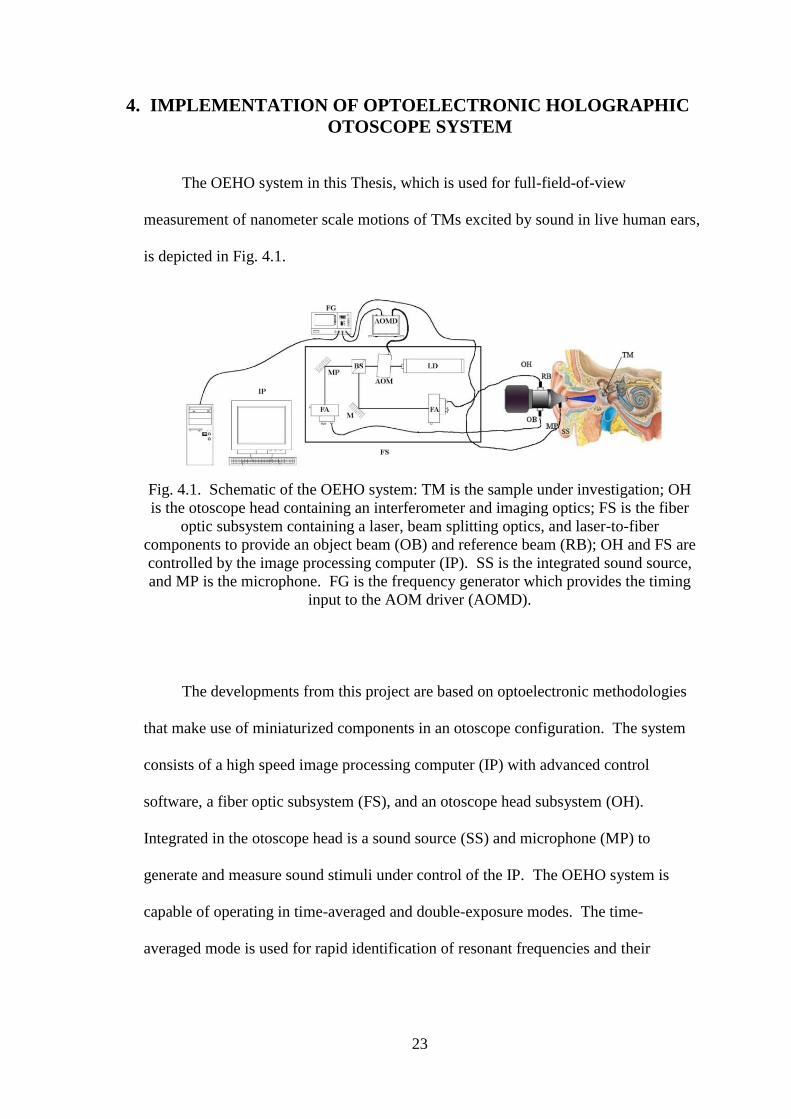
The OEHO system in this Thesis, which is used for full-field-of-view
measurement of nanometer scale motions of TMs excited by sound in live human ears,
is depicted in Fig. 4.1.
Fig. 4.1. Schematic of the OEHO system: TM is the sample under investigation; OH
is the otoscope head containing an interferometer and imaging optics; FS is the fiber
optic subsystem containing a laser, beam splitting optics, and laser-to-fiber
components to provide an object beam (OB) and reference beam (RB); OH and FS are
controlled by the image processing computer (IP). SS is the integrated sound source,
and MP is the microphone. FG is the frequency generator which provides the timing
input to the AOM driver (AOMD).
The developments from this project are based on optoelectronic methodologies
that make use of miniaturized components in an otoscope configuration. The system
consists of a high speed image processing computer (IP) with advanced control
software, a fiber optic subsystem (FS), and an otoscope head subsystem (OH).
Integrated in the otoscope head is a sound source (SS) and microphone (MP) to
generate and measure sound stimuli under control of the IP. The OEHO system is
capable of operating in time-averaged and double-exposure modes. The time-
averaged mode is used for rapid identification of resonant frequencies and their

24
corresponding mode shapes of vibration in samples. Double-exposure mode is used
for determination of the magnitude and phase of nanometer scale motions of the entire
surface of the TMs between two states of deformation.
4.1 Fiber optic subsystem
The fiber optic subsystem (FS) used for transmission and modulation of laser
light is shown in Fig. 4.2.
(a) (b)
(c)
Fig. 4.2. Fiber optic subsystem: (a) schematic model depicting the major components;
(b) CAD model depicting the major components; and (c) fabricated subsystem.

25
In biological samples, light interaction effects, such as reflection, refraction, and
absorption, will diminish the quality of the fringes or contrast, which minimizes the
accuracy of phase measurements. In order to overcome this, suitable methodologies
that will allow improving the phase measurements through the enhancement of fringe
contrasts were investigated. Different light sources, specifically different
wavelengths and powers in combination with specific coating substances were based
on nanoparticles were considered. For this Thesis the light source was chosen as a
solid state laser (LD) with an operational wavelength of 473 nm and a power of 15
mW, and samples were coated with white paint.
As shown in Fig. 4.2a, the output of the laser is directed through an acousto-
optic modulator (AOM) and through the beam splitter (BS), which splits the light into
a reference beam (RB) and an object illumination beam (OB) with an 80:20 power
ratio. The OB is directed to a mirror (M) and RB is directed to another mirror
mounted onto piezoelectric modulators (MPM) to generate the required additional
phase. Both beams are coupled into single mode fibers using laser-to-fiber coupler
assemblies (FA).
4.2 Otoscope head subsystem
The optomechanical design was carried out with commercially available
software [OSLO, 2005] as seen in Fig 4.3, by taking into account the TM anatomy
and the results of preliminary holographic measurements of TM displacements in
several animal species.

26
Fig. 4.3. Ray tracing using commercially available software. So: Object to front
principal point distance, Si: Rear principal point to image distance, DOF: Depth of
field.
The OH subsystem houses a compact interferometer, a high speed CCD camera,
and an imaging system (IS) which includes an achromatic lens and an aperture, and
has characteristic dimensions of 100 x 60 x 120 mm3.
Many innovative, accurate, and commercially available lens systems for use
with cameras or the human eye have been designed as a result of research in optics.
All the information collected by the system comes through the lens. In order to use a
commercially available lens for the OEHO system, specific parameters of the lens
were needed.
Commercially available lenses specify the lens focal length (f), the F/#, which
is a ratio between the lens focal length and diameter. With these two numbers we can
calculate numerical aperture, field of view, and magnification of the image.
The numerical aperture is a dimensionless number, always less than 1, that
describes the angular acceptance of rays of light in an optical element. The following
equations define the relationship between F/#, diameter (Dl) and focal length (f)
[Hecht, 1989]:
𝐹/# =𝑓
𝐷𝑙, (4.1)
27
𝐹/# =1
2.𝑁𝐴, (4.2)
𝑁𝐴 = sin 𝜃, (4.3)
1
𝑓=
1
𝑆𝑜+
1
𝑆𝑖, (4.4)
where NA and are the numerical aperture and the angle of incidence, respectively.
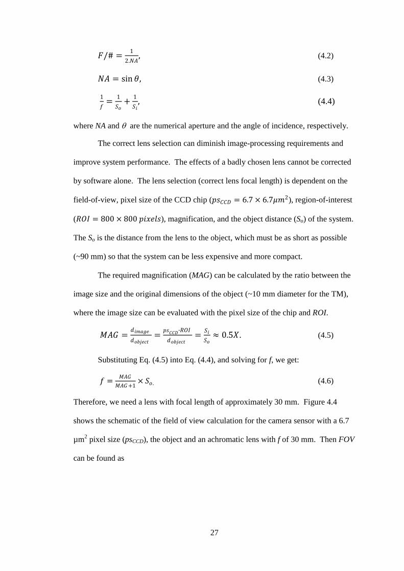
The correct lens selection can diminish image-processing requirements and
improve system performance. The effects of a badly chosen lens cannot be corrected
by software alone. The lens selection (correct lens focal length) is dependent on the
field-of-view, pixel size of the CCD chip (𝑝𝑠𝐶𝐶𝐷 = 6.7 × 6.7𝜇𝑚2), region-of-interest
(𝑅𝑂𝐼 = 800 × 800 𝑝𝑖𝑥𝑒𝑙𝑠), magnification, and the object distance (So) of the system.
The So is the distance from the lens to the object, which must be as short as possible
(~90 mm) so that the system can be less expensive and more compact.
The required magnification (MAG) can be calculated by the ratio between the
image size and the original dimensions of the object (~10 mm diameter for the TM),
where the image size can be evaluated with the pixel size of the chip and ROI.
𝑀𝐴𝐺 =𝑑𝑖𝑚𝑎𝑔𝑒
𝑑𝑜𝑏𝑗𝑒𝑐𝑡=
𝑝𝑠𝐶𝐶𝐷∙𝑅𝑂𝐼
𝑑𝑜𝑏𝑗𝑒𝑐𝑡=
𝑆𝑖
𝑆𝑜≈ 0.5𝑋. (4.5)
Substituting Eq. (4.5) into Eq. (4.4), and solving for f, we get:
𝑓 =𝑀𝐴𝐺
𝑀𝐴𝐺+1× 𝑆𝑜 . (4.6)
Therefore, we need a lens with focal length of approximately 30 mm. Figure 4.4
shows the schematic of the field of view calculation for the camera sensor with a 6.7
µm2 pixel size (psCCD), the object and an achromatic lens with f of 30 mm. Then FOV
can be found as
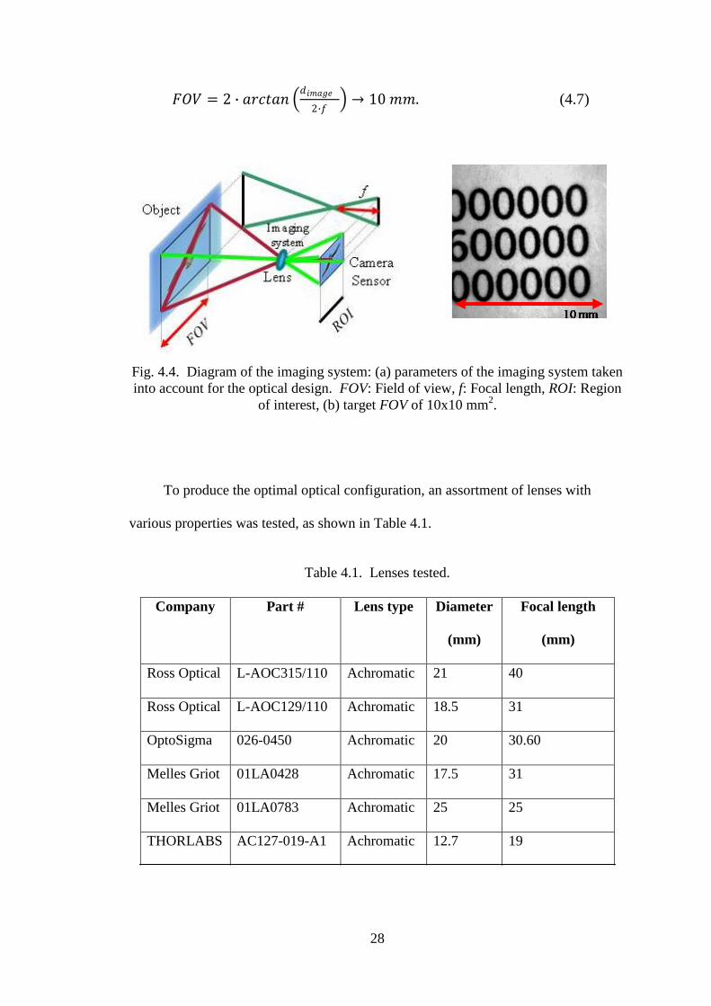
28
𝐹𝑂𝑉 = 2 ∙ 𝑎𝑟𝑐𝑡𝑎𝑛 𝑑𝑖𝑚𝑎𝑔𝑒
2∙𝑓 → 10 𝑚𝑚. (4.7)
Fig. 4.4. Diagram of the imaging system: (a) parameters of the imaging system taken
into account for the optical design. FOV: Field of view, f: Focal length, ROI: Region
of interest, (b) target FOV of 10x10 mm2.
To produce the optimal optical configuration, an assortment of lenses with
various properties was tested, as shown in Table 4.1.
Table 4.1. Lenses tested.
Company Part # Lens type Diameter
(mm)
Focal length
(mm)
Ross Optical L-AOC315/110 Achromatic 21 40
Ross Optical L-AOC129/110 Achromatic 18.5 31
OptoSigma 026-0450 Achromatic 20 30.60
Melles Griot 01LA0428 Achromatic 17.5 31
Melles Griot 01LA0783 Achromatic 25 25
THORLABS AC127-019-A1 Achromatic 12.7 19
29
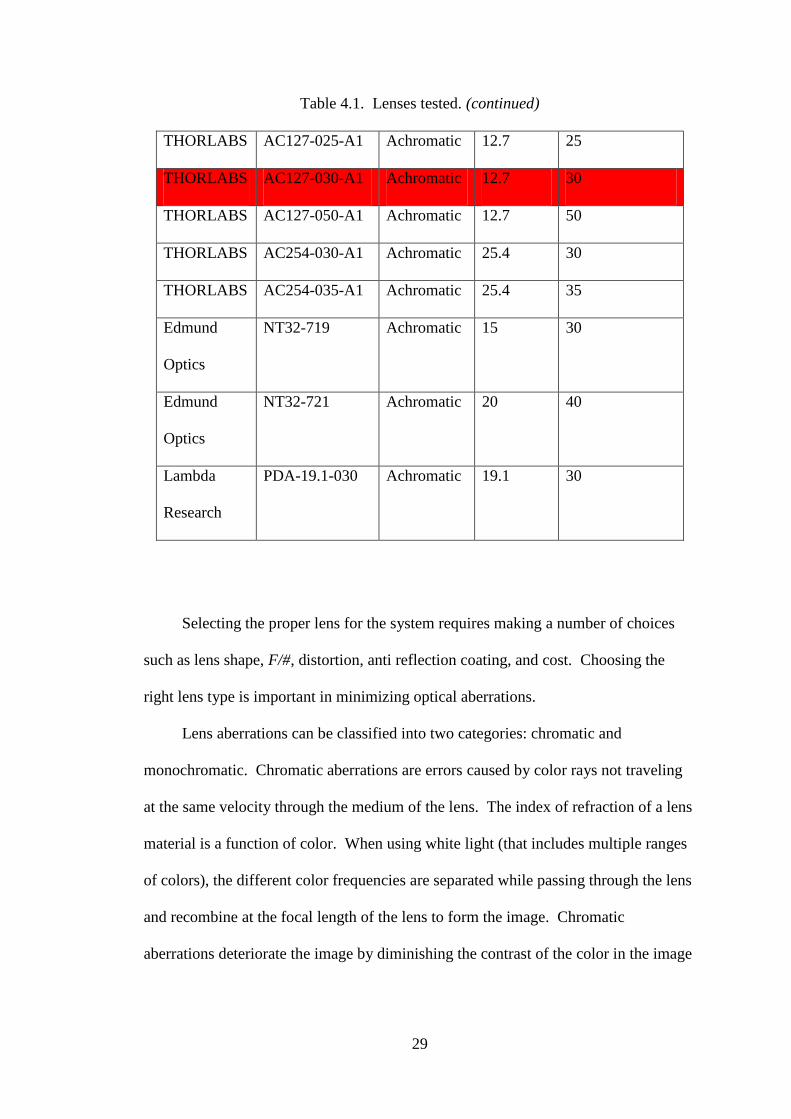
Table 4.1. Lenses tested. (continued)
THORLABS AC127-025-A1 Achromatic 12.7 25
THORLABS AC127-030-A1 Achromatic 12.7 30
THORLABS AC127-050-A1 Achromatic 12.7 50
THORLABS AC254-030-A1 Achromatic 25.4 30
THORLABS AC254-035-A1 Achromatic 25.4 35
Edmund
Optics
NT32-719 Achromatic 15 30
Edmund
Optics
NT32-721 Achromatic 20 40
Lambda
Research
PDA-19.1-030 Achromatic 19.1 30
Selecting the proper lens for the system requires making a number of choices
such as lens shape, F/#, distortion, anti reflection coating, and cost. Choosing the
right lens type is important in minimizing optical aberrations.
Lens aberrations can be classified into two categories: chromatic and
monochromatic. Chromatic aberrations are errors caused by color rays not traveling
at the same velocity through the medium of the lens. The index of refraction of a lens
material is a function of color. When using white light (that includes multiple ranges
of colors), the different color frequencies are separated while passing through the lens
and recombine at the focal length of the lens to form the image. Chromatic
aberrations deteriorate the image by diminishing the contrast of the color in the image
30
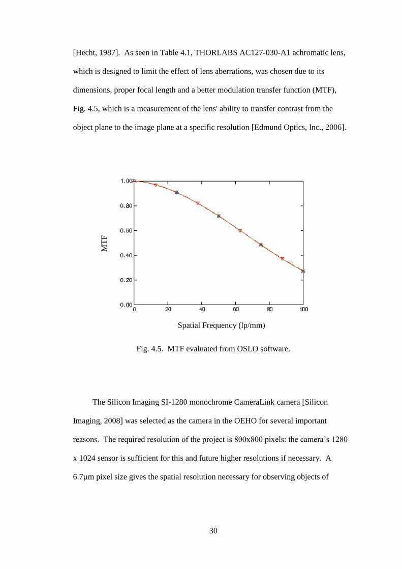
[Hecht, 1987]. As seen in Table 4.1, THORLABS AC127-030-A1 achromatic lens,
which is designed to limit the effect of lens aberrations, was chosen due to its
dimensions, proper focal length and a better modulation transfer function (MTF),
Fig. 4.5, which is a measurement of the lens' ability to transfer contrast from the
object plane to the image plane at a specific resolution [Edmund Optics, Inc., 2006].
Fig. 4.5. MTF evaluated from OSLO software.
The Silicon Imaging SI-1280 monochrome CameraLink camera [Silicon
Imaging, 2008] was selected as the camera in the OEHO for several important
reasons. The required resolution of the project is 800x800 pixels: the camera‟s 1280
x 1024 sensor is sufficient for this and future higher resolutions if necessary. A
6.7µm pixel size gives the spatial resolution necessary for observing objects of
Spatial Frequency (lp/mm)
MT
F
31
interest.
The camera‟s speed is only 30 frames per second at its full resolution, but offers
higher frame rates when using a smaller region of interest. At the 800x800 resolution,
the camera offers up to 80 frames per second which is sufficient for the project. As
opposed to many cameras that only offer 8 or 10-bit image output, the SI-1280 offers
up to 12-bit sampling, giving a much higher dynamic range than an 8 or 10-bit
camera. Finally, the monochromatic version of the camera was selected because it is
preferred for measurements of the laser beams in question.
A very important feature of this camera is its global shutter. As opposed to a
rolling shutter, the global shutter takes a full-frame image. Since some of the aspects
of this project (such as stroboscopic mode) require instantaneous capture, a rolling
shutter would not be sufficient. Because a rolling shutter is more common, the global
shutter was a major contributing factor into selecting the Silicon Imaging SI-1280
camera.
The aperture is used to limit the light entering the imaging system as well as to
control the depth of field (DOF) for proper image focusing properties. Since lasers
output such coherent beams of light, when this beam illuminates an object, the
reflected light will interfere with itself as it is reflected off the surface of the object
creating speckles. These speckles create a random intensity pattern in front of the
object of interest and are highly fluctuating. If the aperture of the lens is decreased,
the speckle size will increase. It was observed that the aperture diameter (Da) should
be at least 5 mm in diameter in order to minimize the speckle effect. In holographic
interferometry, the speckles affect the achievable resolution and accuracy of the
measurement; the size of each speckle is directly proportional to the laser‟s
32
wavelength,
𝑑𝑠𝑝 = 1.22 𝜆𝑆𝑖
𝐷𝑎 , (4.6)
where Da is the size of the aperture, Si is the image distance, and λ is the wavelength
of the laser light.
The OH is enabled with a miniaturized sound source for sample excitation and a
compact microphone for measurements of sound pressure. The sound source is
driven by a frequency generator and the acoustic pressure is recorded with a data
acquisition system.
As shown in Fig. 4.6a, the object illumination beam was coupled to the test
object via a speculum (S). An angled glass window at the back of the speculum
isolates the sound stimulus within the speculum, allowing larger stimulus sound
pressures at lower frequencies. The output of the OB is used to illuminate the sample
of interest while the imaging system (IS) collects the scattered wavefront from the
surface of the samples, the TMs. The image formed by the IS is combined with the
RB by means of the imaging beam splitter (BSI), and directed onto the CCD of the
camera.
Based on the optical design parameters and the synthesized optomechanical
configuration, the OH was fabricated, as shown in Fig. 4.6c. Its optical and imaging
properties are as follows: field-of-view (FOV) of 10 mm2; depth-of-field (DOF) of 5
mm; and magnification of 0.5X.

33
Fig. 4.6. Otoscope head subsystem: (a) schematic model depicting the major
components; (b) CAD models depicting the major components; and (c) fabricated
subsystem.
(c)
(b)
(a)

34
The system resolution was tested with a negative 1951 US Air Force (USAF)
glass target by Edmund Optics because of its surface quality and maximum resolution
(group 7, element 6, i.e. 228lp/mm). Here, negative indicates inversion of the
background and bar colors. Figure 4.7 shows an example of a positive and a negative
target. In the case of a negative target, the bar sets are openings, so the illumination
must come from behind the target in order for the observation system to capture an
image.
Fig. 4.7. USAF 1951 positive and negative target pattern
[Edmund Optics, Inc., 2006].
The target is separated into groups and elements. Each element within a group
corresponds to specific line pair (a set of a black line and a white line) per millimeter.
The specification table of the target can be seen in Fig. 4.8.

35
Fig. 4.8. Specification table for the USAF resolution target
[Edmund Optics, Inc., 2006].
Each group consists of six elements, which are progressively smaller by
𝑙𝑙 =2.5𝑚𝑚
2𝐺𝑟𝑜𝑢𝑝 + 𝐸𝑙𝑒𝑚𝑒𝑛𝑡 −1 /6, (4.7)
where ll is the line length in millimeters for a given group and element [Glynn, 2002].
To get the resolution (the smallest feature that can be resolved by the imaging
system) of the OH subsystem from the chart above, the negative 1951 USAF target
was recorded as depicted in Fig. 4.9.
Since the smallest line pair that we can be distinguished is element 6 from
group 5 that corresponds to 57.0 lp/mm (see Fig. 4.9), where the resolution of the
imaging system is 17 µm (1 over 57.0).
Number of Line Pairs / mm in USAF Resolving Power Test Target 1951
Group Number
Element -2 -1 0 1 2 3 4 5 6 7
1 0.250 0.500 1.00 2.00 4.00 8.00 16.00 32.0 64.0 128.0
2 0.280 0.561 1.12 2.24 4.49 8.98 17.95 36.0 71.8 144.0
3 0.315 0.630 1.26 2.52 5.04 10.10 20.16 40.3 80.6 161.0
4 0.353 0.707 1.41 2.83 5.66 11.30 22.62 45.3 90.5 181.0
5 0.397 0.793 1.59 3.17 6.35 12.70 25.39 50.8 102.0 203.0
6 0.445 0.891 1.78 3.56 7.13 14.30 28.50 57.0 114.0 228.0
Image Format - 1/4 to 228 line pairs/mm Target

36
Fig. 4.9. Recorded USAF 1951 negative glass target with group 5 outlined for
containing the smallest resolvable element set [Edmund Optics, Inc., 2006].
The contrast ratio (C) of the full-field-of-view image is calculated as
𝐶 =𝐼𝑚𝑎𝑥 −𝐼𝑚𝑖𝑛
𝐼𝑚𝑎𝑥 +𝐼𝑚𝑖𝑛, (4.8)
where Imax and Imin are the maximum and minimum interferogram intensity values
respectively. Of the various techniques to find the contrast of an image, the line
profile method, based on the intensity distribution of a line, is used in this
investigation. Though this technique can be performed to calculate contrast in an
image having random intensity profile, it is more reliable when used to calculate the
contrast of a known pattern, such as the USAF target. As explained before, the USAF
target has a sets of black and white lines that corresponds to a square wave profile
having perfect contrast (C = 1) for different spatial frequencies.

37
Figure 4.10 demonstrates the line profile contrast calculation evaluated as
80.85%, indicating an excellent fringe contrast and, consequently high data quality.
[Kreis, 2005]. Figure 4.10a shows an image of G4E2 with a line across the bar set,
while Fig. 4.10b shows the intensity profile of the line and its corresponding contrast
calculated numerically using MATLAB [MatLab 7.0, 2008].
Fig. 4.10. Line profile contrast calculation method (a) image of G4E2 showing a line
profile, (b) line intensity profile and contrast calculation.
Like the body sizes of different species of animals, the tympanic membrane of
various species also varies in size. Different fields-of-view are necessary to
accommodate these varying sizes. Therefore, the placement of the optics inside an
enclosure has to allow for a range of working distances for fields of view of varying
sizes. These limiting distances ultimately define the maximum allowable size of the
enclosure, as shown in Table 4.2.
(b)
Imin=27
(a)
Imax=255

38
Table 4.2. Working distance constraints.
Image distance
Si (mm)
Object distance
So (mm)
Field of View
FOV (mm)
29.7 96.2 11.2
30.4 89.8 10.0
34.3 78.9 8.5
38.9 69.9 6.7

39
5. EVALUATION OF THE OPTOELECTRONIC HOLOGRAPHIC
OTOSCOPE SYSTEM
In order to evaluate the performance of the OEHO system, it was necessary
that the device gathered images that were in fact representative of what was occurring
at the time the image was recorded. To do so, a known geometry with predictable
characteristics was essential to compare and draw conclusions with the experimental
results that were obtained.
Because the geometry of the tympanic membrane is extremely complicated, it
was simplified to a thin circular copper foil (membrane) with a thickness of 0.0254
mm and a diameter of 10 mm. A commercially available sample has the advantage
over machined stock in that the thickness is very precise and the surface finish is
consistent.
The membrane was secured on a piezoelectric shaker for sample excitation,
Fig. 5.1, in a way that ensured uniform boundary conditions which resembled those in
the analytical and computational modes.
Fig. 5.1. A coated copper foil mounted on to the piezoelectric shaker.

40
To secure the foil (membrane) to the piezoelectric shaker, a device had to be
designed and built in steel such a way that the foil could be clamped down between
two surfaces. The base, in order to promote excitation was connected to the piezo.
This provided the surface that the foil was laid on. The top part with a 10 mm hole in
the middle is then placed on the foil.
The membrane was investigated with the OH subsystem set at the designed
magnification of 0.5X, FOV of 10 mm, and a region of interest, ROI, of 800 x 800
pixels. In order to maximize contrast the sample was coated with white paint and the
beam ratio between RB and OB was chosen to be ~ 1.2.
With the OEHO system running in the time-averaged mode and the membrane
excited in the range of 2-8 kHz, fundamental natural frequencies were identified as
depicted in Fig. 5.2 (see p.41). The frequency, starting with an amplitude of 10 volts,
was continuously increased from 100 Hz until the first mode of vibration was reached.
The amplitude was adjusted in order that the deformations were in the range of the
OEHO system. Table 5.1 shows the data acquired for the first 6 modes of vibration of
the copper foil membrane. Analysis of the interferograms indicates contrast of 0.80,
which is suitable for quantitative analysis.
Table 5.1. Membrane test data.
Material Thickness (mm) Coating
Copper 0.0254 White Paint
Modes of
vibration Frequency (Hz) Amplitude (Volts)
1 2150 5.4
2 4100 7.7
3 4470 2.7
4 6600 2.8
5 6630 2.7
6 7290 2.3

41
Fig. 5.2. Time-averaged interferograms of a test copper sample.
5.1. Analytical results
For the purpose of understanding the patterns within the Fig. 5.2, an analytical
model of a circular, homogeneous, isotropic plate (membrane), undergoing free
vibration which is clamped at the edges was developed. In this section, all of the
following assumptions and equations (Eq. (5.1) through Eq. (5.16)) were compiled
from derivations contained in the references McLachlan [1961] and Reddy [1999].
The equation of motion of an isotropic plate can be described as
𝐷∇2∇2W + 𝐤W − Piω2W + Riω
2∇2W = 0 (5.1)
where 𝐷 is the flexural rigidity, 𝐤 is the elastic modulus of the plate. The circular
frequency and the deformation equation of the plate are represented as ω, 𝑊,
respectively. Also, Pi and Ri are the principal and rotary inertia of the plate in which
the rotary inertia (Ri) contributes little to the fundamental frequency so it can be
simplified from the equation of motion
42
∇4 − 𝛽4 𝑊 = 0 (5.2)
where
𝛽4 =P i𝜔
2−𝑘
𝐷 (5.3)
Equation (5.2) can be factored and the solution can be achieved by
superimposing the solutions of the equations indicated in Eq. (5.4)
∇2𝑊1 + 𝛽2𝑊1 = 0, and ∇2𝑊2 + 𝛽2𝑊2 = 0. (5.4)
The solution to Eq. (5.2) is in the form of Fourier series
𝑊 𝑟, 𝜃 = 𝑊𝑛 𝑟 cos 𝑛𝜃 +∞𝑛=0 𝑊𝑛
∗ 𝑟 sin 𝑛𝜃.∞𝑛=1 (5.5)
By substituting Eq. (5.5) into Eq. (5.4) gives the following identical equations for
𝑊𝑛1 and 𝑊𝑛2:
𝑑2𝑊𝑛1
𝑑𝑟 2+
1
𝑟
𝑑𝑊𝑛1
𝑑𝑟−
𝑛2
𝑟2− 𝛽2 𝑊𝑛1 = 0 (5.6)
and
𝑑2𝑊𝑛2
𝑑𝑟 2+
1
𝑟
𝑑𝑊𝑛2
𝑑𝑟−
𝑛2
𝑟2− 𝛽2 𝑊𝑛2 = 0 (5.7)
Both Eqs (5.6) and (5.7) are in the form of Bessel‟s equation and have the solutions as
𝑊𝑛1 = 𝐴𝑛𝐽𝑛 𝛽𝑟 + 𝐵𝑛𝑌𝑛 𝛽𝑟 and,
𝑊𝑛2 = 𝐶𝑛𝑍𝑛 𝛽𝑟 + 𝐷𝑛𝐾𝑛 𝛽𝑟 (5.8)
where 𝐽𝑛 and 𝑌𝑛 are Bessel functions of the first and second kind respectively, and
correspondingly, 𝑍𝑛 and 𝐾𝑛 are the modified Bessel functions of the first and second
kind. 𝐴𝑛 , 𝐵𝑛 , 𝐶𝑛 , and 𝐷𝑛 are the coefficients used to determine the mode shapes by
applying the boundary conditions.
Hence, the general solution of Eq. (5.2) is

43
𝑊 𝑟, 𝜃 = (5.9)
𝐴𝑛𝐽𝑛 𝛽𝑟 + 𝐵𝑛𝑌𝑛 𝛽𝑟 + 𝐶𝑛𝑍𝑛 𝛽𝑟 + 𝐷𝑛𝐾𝑛 𝛽𝑟 cos 𝑛𝜃∞𝑛=0
+
𝐴𝑛∗ 𝐽𝑛 𝛽𝑟 + 𝐵𝑛
∗𝑌𝑛 𝛽𝑟 + 𝐶𝑛∗𝑍𝑛 𝛽𝑟 + 𝐷𝑛
∗𝐾𝑛 𝛽𝑟 sin 𝑛𝜃∞𝑛=1
For solid circular plate, the terms including the modified Bessel functions, 𝑌𝑛
and 𝐾𝑛 , are neglected as they would result in infinite values of deflection at the center
of the membrane. Additionally, assuming that the solution is symmetric, any terms
containing sin 𝑛𝜃 are neglected as well. This results in the following equation as the
𝑛th term of Eq. (5.9):
𝑊𝑛 𝑟, 𝜃 = 𝐴𝑛𝐽𝑛 𝛽𝑟 + 𝐶𝑛𝑍𝑛 𝛽𝑟 cos 𝑛𝜃. (5.10)
The boundary conditions for a clamped circular plate can be considered as
𝑊𝑛 = 0 and 𝜕𝑊𝑛
𝜕𝑟= 0 at 𝑟 = 𝑎 for any 𝜃 (5.11)
and applying these boundary conditions to Eq. (5.10) we obtain
𝐽𝑛 𝛾 𝑍𝑛 𝛾
𝐽𝑛′ 𝛾 𝑍𝑛
′ 𝛾
𝐴𝑛
𝐶𝑛 =
00 (5.12)
where 𝛾 = 𝛽𝑟 evaluated at 𝑟 = 𝑎 and the prime represents differentiation with respect
to 𝛽𝑟. Setting the determinant of the coefficient matrix in Eq. (5.12) to zero yields
the following which is called the frequency equation
𝐽𝑛 𝛾 𝑍𝑛+1 𝛾 + 𝑍 𝛾 𝐽𝑛+1 𝛾 = 0 (5.13)
The roots 𝛾 can be approximated by using the asymptotic series for the Bessel
functions as
𝛾𝑛 ,𝑚 ~𝜃 −4𝑛2−1
8𝜃 1 +
1
𝜃+
28𝑛2+17
48𝜃2+
3 4𝑛2−1
8𝜃3+
83𝑛4+54.5𝑛2+161.19
120𝜃4+ ⋯ (5.14)
44
where 𝜃 = 2𝑚+𝑛 𝜋
2 for 𝑚 ≥ 1, 𝑚 is the rank of the root and 𝑛 is the order of the root.
Now, looking back at the definition of 𝛽 in Eqn. (5.3), simple algebra can be used to
develop an equation for determining the frequencies:
𝜔2 =𝐷𝛽4+𝑘
P i (5.15)
Assuming that the membrane foundation is rigid 𝑘 = 0 and substituting 𝛽 with 𝛾
𝑎
results in the final equation for determining the frequency of vibration
𝜔 =𝜆2
𝑎2 𝐷
P i (5.16)
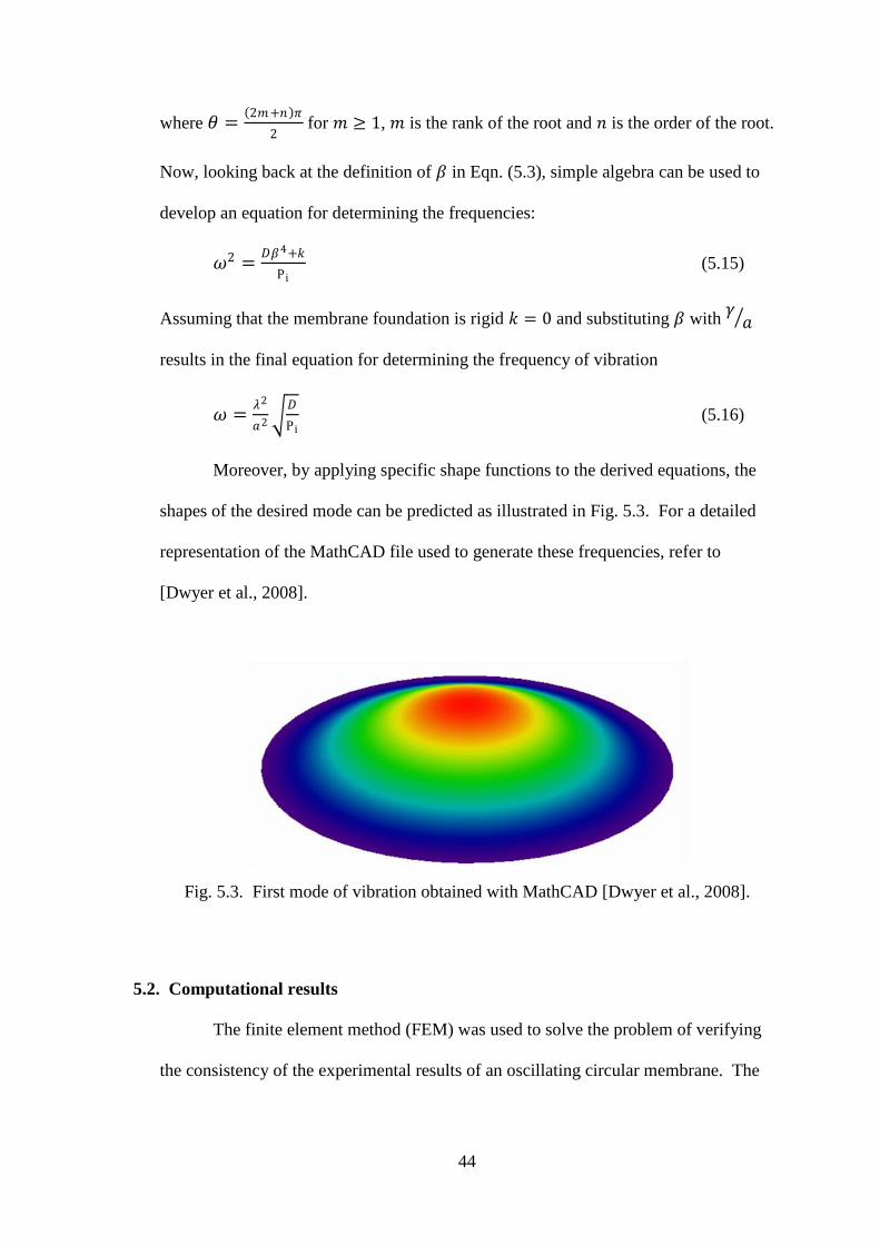
Moreover, by applying specific shape functions to the derived equations, the
shapes of the desired mode can be predicted as illustrated in Fig. 5.3. For a detailed
representation of the MathCAD file used to generate these frequencies, refer to
[Dwyer et al., 2008].
Fig. 5.3. First mode of vibration obtained with MathCAD [Dwyer et al., 2008].
5.2. Computational results
The finite element method (FEM) was used to solve the problem of verifying
the consistency of the experimental results of an oscillating circular membrane. The

45
finite element program, Abaqus/CAE version 6.7 was used to model the oscillating
membrane [Dwyer et al., 2008].
A 3D deformable solid with a diameter of 10 mm and a thickness of 0.0254
mm was made of the membrane. The material property of the copper with a density
of 8960kg/m3, a Young‟s Modulus of 110 GPa and a Poisson‟s ratio of 0.343. A
solid, homogeneous section was created and assigned to the entire membrane. A
boundary condition was placed on the circumference of the membrane constraining
movement in the x, y and z directions.
Results were obtained for the first six modes of vibration as shown in Fig. 5.4.
A deformed contour plot on each of these six modes was created. Both the frequency
and the shape of each individual mode were used to validate the data which had been
obtained from the experimental and computational methods.
Fig. 5.4. Finite element method results for natural frequencies of a test copper sample
[Dwyer et al., 2008].
46
5.3. Results comparisons
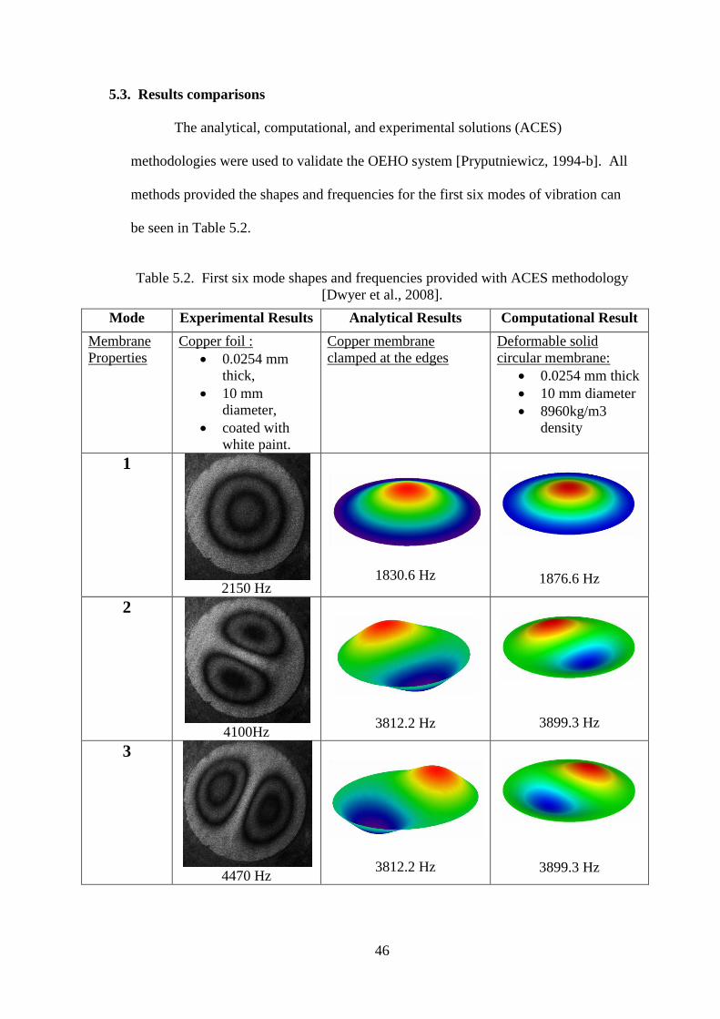
The analytical, computational, and experimental solutions (ACES)
methodologies were used to validate the OEHO system [Pryputniewicz, 1994-b]. All
methods provided the shapes and frequencies for the first six modes of vibration can
be seen in Table 5.2.
Table 5.2. First six mode shapes and frequencies provided with ACES methodology
[Dwyer et al., 2008].
Mode Experimental Results Analytical Results Computational Result
Membrane
Properties
Copper foil :
0.0254 mm
thick,
10 mm
diameter,
coated with
white paint.
Copper membrane
clamped at the edges
Deformable solid
circular membrane:
0.0254 mm thick
10 mm diameter
8960kg/m3
density
1
2150 Hz
1830.6 Hz
1876.6 Hz
2
4100Hz
3812.2 Hz
3899.3 Hz
3
4470 Hz
3812.2 Hz
3899.3 Hz
47
Table 5.2. First six mode shapes and frequencies provided with ACES methodology
[Dwyer et al., 2008]. (continued)
Mode Experimental Results Analytical Results Computational Result
Membrane
Properties
Copper foil :
0.0254 mm
thick,
10 mm
diameter,
coated with
white paint.
Copper membrane clamped
at the edges
Deformable solid
circular membrane:
0.0254 mm
thick
10 mm diameter
8960kg/m3
density
4
6600 Hz
6256.3 Hz
6381.8 Hz
5
6630 Hz
6256.3 Hz
6381.8 Hz
6
7290 Hz
7128.6 Hz
7329.9 Hz
As demonstrated in Table 5.3, the error between the experimental,
computational and analytical was calculated [Dwyer et al., 2008].
48
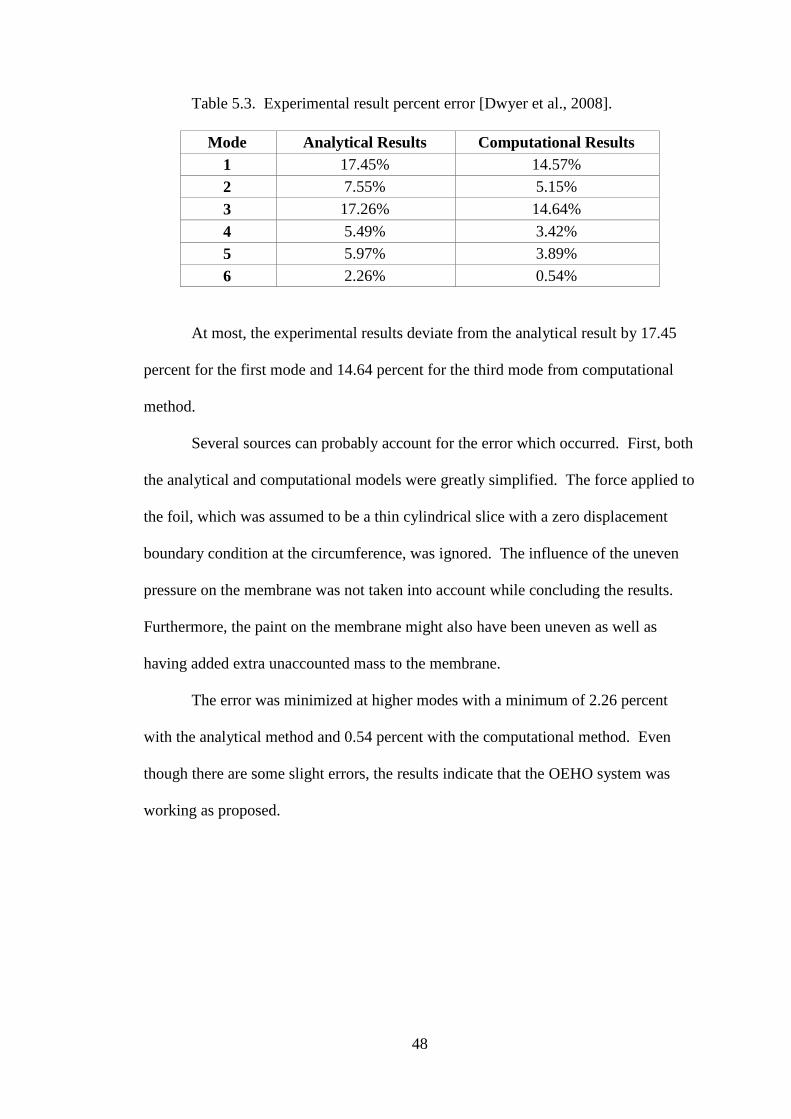
Table 5.3. Experimental result percent error [Dwyer et al., 2008].
Mode Analytical Results Computational Results
1 17.45% 14.57%
2 7.55% 5.15%
3 17.26% 14.64%
4 5.49% 3.42%
5 5.97% 3.89%
6 2.26% 0.54%
At most, the experimental results deviate from the analytical result by 17.45
percent for the first mode and 14.64 percent for the third mode from computational
method.
Several sources can probably account for the error which occurred. First, both
the analytical and computational models were greatly simplified. The force applied to
the foil, which was assumed to be a thin cylindrical slice with a zero displacement
boundary condition at the circumference, was ignored. The influence of the uneven
pressure on the membrane was not taken into account while concluding the results.
Furthermore, the paint on the membrane might also have been uneven as well as
having added extra unaccounted mass to the membrane.
The error was minimized at higher modes with a minimum of 2.26 percent
with the analytical method and 0.54 percent with the computational method. Even
though there are some slight errors, the results indicate that the OEHO system was
working as proposed.

49
6. OPTOELECTRONIC HOLOGRAPHIC OTOSCOPE SYSTEM IN
MEDICAL ENVIRONMENT
After the OEHO system was evaluated, it was deployed at the Massachusetts
Eye and Ear Infirmary (MEEI) so that it could be used and evaluated under medical
testing conditions for investigation and inspection of TMs, Fig.6.1.
(a)
(b) (c)
Fig. 6.1. OEHO system installation: (a) OEHO system at MEEI; (b) otoscope head
subsystem testing post mortem human temporal bone at MEEI; and (c) otoscope head
subsystem testing post mortem chinchilla at MEEI.

50
6.1. Experimental results in tympanic membrane
In MEEI, both time-averaged holography and double-exposure holography
measurements are being used and it has been observed that the OEHO system has a
high mechanical stability while providing high quality images.
Several different sample types were prepared for use with the OEHO system.
The test samples were acoustically excited using a speculum designed specifically to
direct sound at the test samples. Figure 6.2 illustrates the time-averaged holography
images of sound-induced TM displacements of a cadaveric human, a cadaveric
chinchilla, live chinchilla and cadaveric cat, in the frequency range of 400 Hz to
25 kHz. The sound intensities, noted as dB SPL, were chosen to produce a moderate
level of sound stimulation in each image.
At the top of each column is an illustration depicting the orientation of the
exposed TM surface (the gray area). The frequency of excitation increases from top
to bottom. The TM and manubrium are outlined in black, and the umbo is marked
“U”. The thick horizontal line protruding from the top of the holograms of the
chinchilla, and on the cat TM images there is the shadow of the probe tube used to
measure the sound level of the stimulus.
Increasing displacements are indicated by the corresponding fringe densities.
At frequencies less than 1 kHz, the TM displacement patterns are “simple”. These
displacements are characterized by one or two regions of maximal displacement.
These patterns are consistent with the previous results taken in 1972 from Tonndorf
and Khanna [Tonndorf and Khanna, 1972]. At 4 kHz in cat and human, and near
1 kHz in the chinchilla, the TM displacement patterns are “complex,” and these
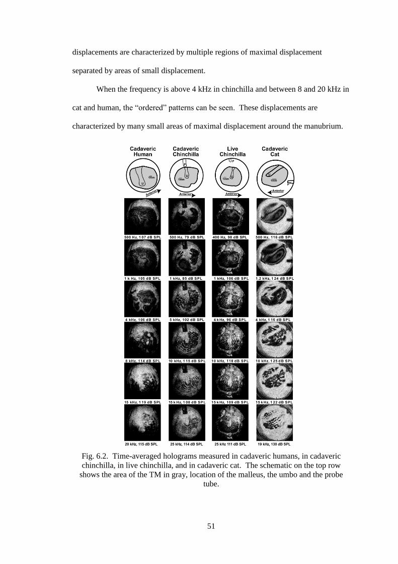
51
displacements are characterized by multiple regions of maximal displacement
separated by areas of small displacement.
When the frequency is above 4 kHz in chinchilla and between 8 and 20 kHz in
cat and human, the “ordered” patterns can be seen. These displacements are
characterized by many small areas of maximal displacement around the manubrium.
Fig. 6.2. Time-averaged holograms measured in cadaveric humans, in cadaveric
chinchilla, in live chinchilla, and in cadaveric cat. The schematic on the top row
shows the area of the TM in gray, location of the malleus, the umbo and the probe
tube.

52
Double-exposure holography was used for quantitative measurements of the
displacements of TM with nanometer resolution. With introducing stroboscopic
illumination, any single hologram from the sample can be frozen at any point of its
vibrating cycle by illuminating the object with short stroboscopic pulses, which can
be adjusted with the duty cycle of the stroboscopic pulse (1/10 of the tonal excitation
period), synchronized with the selected phase of the vibration excitation, Fig. 6.3.
Stroboscopic illumination was obtained by means of an AOM placed in the laser
beam before BS, see Fig. 4.1. Voltage pulses were applied to the AOM in synchrony
with the sample excitation. These pulses were supplied by a frequency generator (FG)
which permitted adjustment of the duty cycle of the stroboscopic pulse and its phase
with respect to the tonal excitation.
Fig. 6.3. Synchronization of the illumination with the object excitation.
The holograms were processed using the phase stepping technique in order to
extract the phase map depicting the sample displacement. Moreover, Figs 6.4, 6.5 and
6.6 show the difference in human temporal bone displacement between two stimulus
53
phase, both in 2D and 3D, at 500 Hz, 800 Hz, 4 kHz, 12 kHz, 15 kHz, and 20 kHz,
respectively.
The colors changing between green and red code represents inward
displacements of TM surface where as the colors varying between green and purple
code is outward motions. The peak-to-peak surface out of plane displacement is on
the order of 90nm, 120 nm, 190 nm, 150 nm, 210 nm, and 60 nm, respectively.

54
Fig. 6.4. Full-field-of-view stroboscopic holography measurements in human
temporal bone at 500 Hz, showing a peak-to-peak surface out of plane displacement
on the order of 90nm: (a) unwrapped phase (2D plot); and (b) 3D plot.
(a)
(b)

55
Fig. 6.5. Full-field-of-view stroboscopic holography measurements in human
temporal bone at 800 Hz, showing a peak-to-peak surface out of plane displacement
on the order of 120nm: (a) unwrapped phase (2D plot); and (b) 3D plot.
(a)
(b)

56
Fig. 6.6. Full-field-of-view stroboscopic holography measurements in human
temporal bone at 4 kHz, showing a peak-to-peak surface out of plane displacement on
the order of 190nm: (a) unwrapped phase (2D plot); and (b) 3D plot.
(a)
(b)

57
Fig. 6.7. Full-field-of-view stroboscopic holography measurements in human
temporal bone at 12 kHz, showing a peak-to-peak surface out of plane displacement
on the order of 150nm: (a) unwrapped phase (2D plot); and (b) 3D plot.
(a)
(b)

58
Fig. 6.8. Full-field-of-view stroboscopic holography measurements in human
temporal bone at 15 kHz, showing a peak-to-peak surface out of plane displacement
on the order of 210nm: (a) unwrapped phase (2D plot); and (b) 3D plot.
(a)
(b)
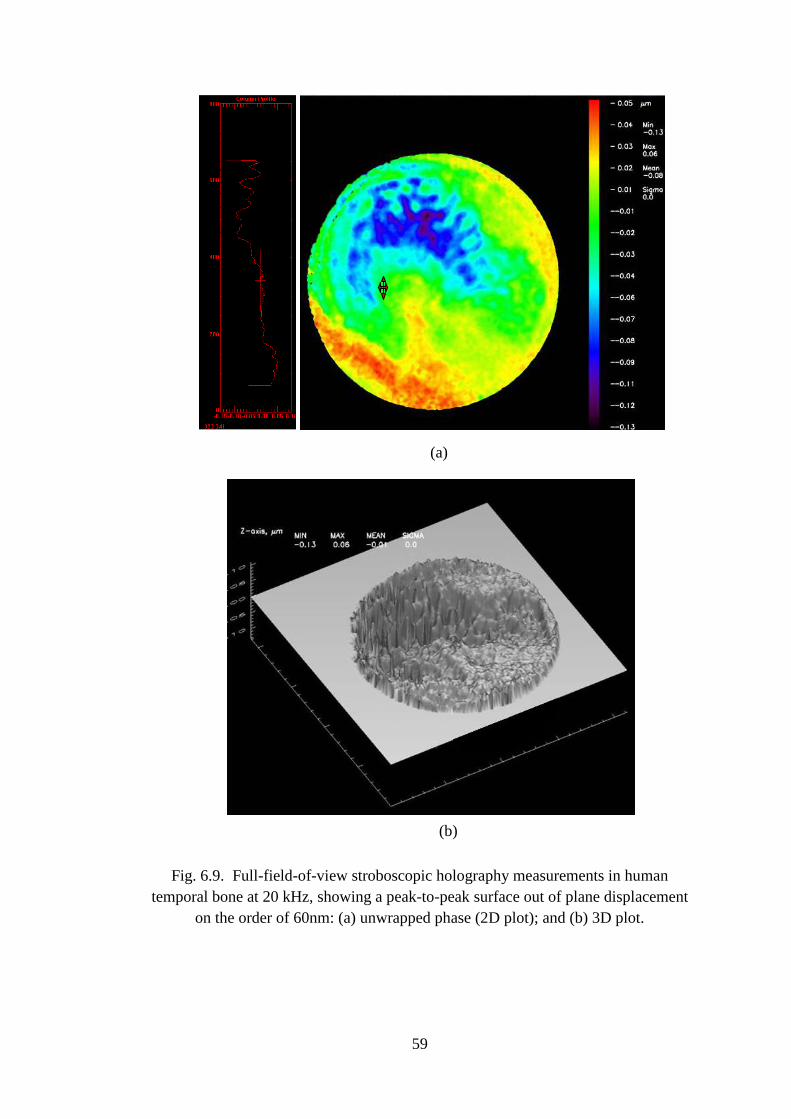
59
Fig. 6.9. Full-field-of-view stroboscopic holography measurements in human
temporal bone at 20 kHz, showing a peak-to-peak surface out of plane displacement
on the order of 60nm: (a) unwrapped phase (2D plot); and (b) 3D plot.
(a)
(b)

60
7. CONCLUSIONS AND FUTURE WORK
This Thesis has demonstrated the feasibility of the compact OEHO system for
characterization of sound induced, nanometer scale deformations in the TM.
The OEHO system, operated in time-averaged and double-exposure modes, has been
used to obtain measurements of TM behavior in three post mortem mammalian
species: cat, chinchilla (including one live chinchilla) and human. Time-averaged
holography used to determine the modes of vibration of all the species; double-
exposure holography was applied to human temporal bone to obtain quantitative full-
field-of-view measurements of deformations with nanometer resolution.
To illustrate measurement capabilities of the system, we have shown
representative results of post-mortem and live chinchilla TM at frequencies of up to
25 kHz. The observed vibrations include simple, complex and ordered displacement
patterns. However, the significance of this has yet to be understood.
The physiology of different species and the preliminary holographic
measurements of TM motion were taken into account and dictated by the
optomechanical parameters of the OEHO system. The following parameters
characterize the OEHO configuration: FOV of 10 mm, DOF of 5 mm, MAG of 0.5X,
C of 0.80 obtained with the beam ratio of 1.2 and resolution of 57.0 lp/mm.
The significance of the measurements presented demonstrates the applicability
and validity of the OEHO systems. The most important fact was that the
measurements, as presented, showed that the behavior of the TM had not been
observed and quantified previously especially at such high frequencies.
61
Before being used in a medical research environment, a test was employed to
evaluate the image quality and resolution by using finite element analysis, analytical
and experimental solutions.
Further miniaturization of the OH subsystem by the use of MEMS technologies
and advanced software tools for optomechanical design, analysis and manufacturing
will continue. Challenges that are expected range from investigations on the
fundamentals of laser-to tissue interaction, to improve and develop high-speed digital
holographic algorithms.
Moreover, the OEHO system will be used to attempt answering fundamental
questions related to the shape and function of the TM, the effects of middle-ear in
hearing capabilities, the effects of perforations in TM, and the determination of
mechanical properties of the TM.

62
8. REFERENCES
Allen, J. B., Jeng, P. S., and Levitt, H., 2005, “Evaluation of human middle ear
function via an acoustic power assessment,” JRRD, 42(4):63-78.
Castellini, P., Revel, G. M., and Tomasini, E. P., 1998, “Laser doppler vibrometry: A
review of advances and applications,” The Shock and Vibration Digest,
30(6):443-456.
Castellini, P., MArtarrelli, M., and Tomasini, E. P., 2006, “Laser doppler vibrometry:
Development of advanced solutions answering to technology‟s needs,”
Science Direct, 20:1265-1285
Csillag, A., 2005, Atlas of the sensory organs: functional and clinical anatomy, 1st
ed., Human press, Totowa, New Jersey.
Dwyer, B. W., Maccaferri, M. E., and Wester, C. R., 2008, Design and realization of
a laser holographic otoscope, Department of Mechanical Engineering,
Worcester Polytechnic Institute, Worcester, MA.
Dirckx, J. J. J., and Decraemer, W. F., 2000, “Interferometer for eardrum shape
measurement, based on projection of straight line rulings,” Lasers Med Sci,
15:131–139.
Edmund Optics, Inc., Edmund Optics, Inc., Barrington, NY, 2006.
Fay, J., Puria. S., Decraemer, W. F., and Steele, C., 2005, “Three approaches for
estimating the elastic modulus of the tympanic membrane,” J. Biomech.,
38(9):1807-1815.
Feeney, M.P., Grant, I. L., and Marryott, L.P., 2003, “Wideband energy reflectance in
adults with middle-ear disorders,” J. Sppech Lang. Hear. Res., 46:901-911.
Fundamentals of hearing, http://www.mne.psu.edu/lamancusa/me458/2_hearing.pdf,
63
(last accessed: 19 August 2008).
Funnell, W. R., and Laszlo, C. A., 1978, “Modeling of the cat eardrum as a thin shell
using the finite-element method,” J. Acoust. Soc. Am., 63(5):1461-1467.
Furlong, C., and Pryputniewicz, R. J., 1996, “Hybrid experimental and computational,
investigation of mechanical components,” SPIE, 2861:13-24.
Furlong, C., and Pryputniewicz, R. J., 1998, “Hybrid computational and experimental
approach for the study and optimization of mechanical components,” J. Opt.
Eng., 37(5):1448-1455,
Furlong, C., and Pryputniewicz, R. J., 1998, “Electro-optic holography method for
determination of surface shape and deformation,” SPIE, 3478:86-97.
Furlong, C., Yokum, J. S., and Pryputniewicz, R. J., 2002, “Sensitivity, accuracy, and
precision issues in opto-electronic holography based on fiber optics and high-
spatial and high-digital resolution cameras,” Proc. Internat. Conf, on
Measurements in Advanced Materials and Systems, Milwaukee, WI.
Furlong, C., Rosowski, J. J., Hulli, N., and Ravicz, M. E., 2007, “Preliminary
analyses of tympanic-membrane motion from holographic measurements,”
Proc. SEM, Selected Paper from the 8th ISMAN.
Furlong C., Hernández-Montes, M. S., Hulli, N., Cheng, J. T., Ravicz M. E., and
Rosowski J. J., 2008, “Development of an optoelectronic holographic
otoscope for characterization of sound-induced displacements in tympanic
membranes,” 31st Midwinter Meeting of the Association for Research in
Otolaryngology, Phoenix, Az.
Furlong, C., Rosowski, J. J., Hulli, N., and, Ravicz, M., 2008, “Preliminary analyses
of tympanic-membrane motion from holographic measurements,” Strain, in-
64
press.
Glynn, E., “USAF and microscopy resolution test charts and pixel profiles,”
http://www.efg2.com/Lab/ImageProcessing/TestTargets/,
(last accessed: 20 November 2008)
Grundman, J., and Wigton, R., “Tympanic membrane evaluation”, in Ear
Examination, http://webmedia.unmc.edu/intmed/general/eye&ear/introtm.htm,
(last accessed: 19 August 2008).
Hecht, E., 1989, Optics, 2nd
ed., Addison-Wesley Publishing Company.
Hernández-Montes, M. S., Furlong, C., Rosowski, J. J., Hulli, N., and Harrington, E.,
2008, “ Optoelectronic holographic otoscope for measurement of nano-
displacements in tympanic membranes,” Proc. SEM.
Holophile, Inc., “History of holography,” http://www.holophile.com/history.htm,
(last accessed: 19 August 2008).
Huber, A. M., Schwab, C., Linder, T., Stoeckli, S. J., Ferrazzini, M., Diller N., and
Fisch U., 2001, “Evaluation of eardrum laser Doppler interferometry as a
diagnostic tool,” Laryngoscope, 111(3):501-507.
Hulli, N., Franco, R. A., Rodriguez-Vera, R., and Furlong, C., 2007, “Development of
an optoelectronic, high-speed, 3D shape measurement system for medical
applications, ” Proc. SEM.
Katz, J., 1994, Handbook of Clinical Audiology, 4th
ed., Williams & Wilkins,
Baltimore, Maryland.
Keefe, D. H., Bulen, J. C., Arehart, K. H., and Burns, E. M., 1993, “Ear-canal
impedance and reflection coefficient in human infants and adults,” J. Acoust.
Soc. Am., 94(5):2617-2638.
65
Khanna, S. M., and Tonndorf, J., 1972, “Tympanic membrane vibrations in cats
studied by time-averaged holography,” J. Acoust. Soc. Am., 51(6): 1904-1920.
Kreis, T., 2005, Handbook of holographic interferometry, Wiley-VCH, Weinheim,
Germany.
Kuypers, L. C., Decraemer, W. F., and Dirckx J. J. J, 2006, „Thickness distribution of
fresh and preserved human eardrums measured with confocal microscopy,”
Otol Neurotol, 27(2): 256-264.
Lim, D. J., 1970, “Human tympanic membrane, an ultrastructural observation,” Acta
Otolaryngol., 70(3):176-186.
Lim, D. J., 1995, “Structure and function of the tympanic membrane: a review,” Acta
otorhinolaryngol. Belg., 49(2):101-115.
Løkberg, O. J., Høgmonen, K., and Gundersen, T., 1980, “Vibration measurement of
the human tympanic membrane – in vivo,” Acta Otolaryngol., 89(1-2):37-42.
Margolis, R. H., Saly, G. L., and Keefe, D. H., 1999, “Wideband reflectance
tympanometry in normal adults,” J. Acoust. Soc. Am., 106(1):265-280.
McLachlan, N.W., 1961, Bessel Functions for Engineers, Oxford University Press,
Amen House, London E.C.4.
MatLab 7.0, The Mathworks, Natick, MA, 2008.
Mikoklai, T. K., Duffey, J., and Adlin, D., “A guide to tympanometry for hearing,”
http://www.maico-
diagnostics.com/eprise/main/Maico/Products/Files/MI24/Guide.Tymp.pdf,
(last accessed: 19 August 2008).
OSLO software for opto-mechanical modeling, Optics Reference , Lambda Research
Corporation, Littleton MA, 2005.

66
Pryputniewicz, R. J., and Stetson, K. A., 1980, “Determination of sensitivity vectors
in hologram interferometry from two known rotations of the object,” Appl.
Opt., 19:2201-2205
Pryputniewicz, R. J., 1985, “Time average holography in vibration analysis,” Opt.
Eng., 24(5):843-848.
Pryputniewicz, R. J., 1987, “Quantitative interpretation of time-average holograms in
vibration analysis,” Optical metrology, in NATO Advanced Science Institute
(ASI) Series, Porto, Portugal, pp. 296-371.
Pryputniewicz, R. J., 1989, “Measurement of vibration patterns using electro-optic
holography,” SPIE, 1162:456-467
Pryputniewicz, R. J., 1994-a, “Quantitative determination of displacements and strains
from holograms,” in Holographic Interferometry, P. K. Rastogi, ed., Springer-
Verlag, Berlin, pp. 33-72.
Pryputniewicz, R. J., 1994-b, “A hybrid approach to deformation analysis,”
SPIE, 2342:282-296.
Pryputniewicz, R. J., 1996, Holographic numerical analysis, ME/CHSLT-NEST,
Worcester Polytechnic Institute, Worcester, MA.
Pryputniewicz, R. J., Yokum, J. S., and Furlong, C., 2002, “Optoelectronic
holography method for measurements of absolute inside shapes of objects,”
Proc. 2002 Internat. Conf. on Measurements in Advanced Materials and
Systems, SEM, Milwaukee, WI.
Reddy, J.N., 1999 Theory and Analysis of Elastic Plates, Taylor & Francis, 325
Chestnut Street, Philadelphia, PA 19106.
Robinson, D. W., and Reid, G. T., 1993, Interferogram analysis, digital fringe pattern

67
measurement techniques, 1st ed., Taylor & Francis, England, pp. 23-71.
Rosowski, J. J., Carney, L. H, Lynch, T. J., and Peake, W. T., 1986, “The
effectiveness of external and middle ears in coupling acoustic power into the
cochlea,” in: Peripheral Auditory Mechanisms, Allen, J. B., Hall, J. L.,
Hubbard, A., Neely, S. T., and Tubis, A., eds, New York, Springer-Verlag,
pp. 3-12.
Rosowski, J. J., 1996, “Models of external- and middle- ear function,” in: Auditory
computation, Hawkins, H. L., McMullen, T. A., Popper A. N., and Fay, R. R.,
eds, Springer-Verlag New York, Inc., NY, pp 15-60.
Rosowski, J. J., Nakajima, H. H., and, Merchant, S. N., 2008, “Clinical utility of
laser-doppler vibrometer measurements in live normal and pathologic human
ears,” Ear & Hearing, 29(1):3-19.
Sanna, M., Sunose H., Mancini, F., Russo, A., and Taibah, A., 2003, Middle ear and
mastoid microsurgery, Georg Thierne Verlag, Stuttgart, Germany, pp.1-15.
Schubert, E. D., 1980 Hearing: Its function and dysfunction, Springer-Verlag, New
York, NY.
Shanks, J. E., Lilly, D. J., Margolis, R. H., Wiley, T. L., and Wilson, R. H., 1988,
“Tympanometry,” J. Speech and Hearing Disorders, 53:354-377.
Silicon Imaging SI 1280F Mega Camera,
http://www.alacron.com/camera/machine%20vision%20cameras/Silicon%20I
maging/SI_Silicon%20imaging_SI-1280F.pdf, (last accessed: 19 November
2008).
Sundberg, M.,2008, Optical methods for tympanic membrane characterization
towards objective otoscopy in otitis media, Department of Biomedical
68
Engineering, Linköpings universitet, Linköping Dissertation No. 1173,
Linköping, Sweden, pp.19-21.
Tonndorf, J., and Khanna, S. M., 1970, “The role of the tympanic membrane in
middle ear transmission,” Ann. Otol. Rhinol. Laryngol, 79(4):743-753.
Tonndorf, J., and Khanna, S. M., 1971, “The tympanic membrane as a part of the
middle ear transformer,” Acta Otolaryngol., 71(2):177-180.
Tonndorf, J., and Khanna, S. M., 1972, “Tympanic-membrane vibrations in human
cadaver ears studied by time-averaged holography,” J. Acoust. Soc. Am.,
52(4):1221-1233.
Vest, M. C., 1979, Holographic Interferometry, John Wiley & Sons.
Wada, H., Kobayashi, T., Suetake, M., and Tachizaki, H.,1989, “Dynamic behavior of
the middle ear based on sweep frequency tympanometry,” Audiology., 28:127-
134.
Wada, H., Ando, M., Takeuchi, M., Sugawara, H., and Koike, T., 2002, “Vibration
measurement of the tympanic membrane of guinea pig temporal bones using
time averaged speckle pattern interferometry,” J. Acoust. Soc. Am.,
111(5):2189-2199.
Whittemore, K. R., Merchant, S. N., Poon B. B., and Rosowski, J. J., 2004, “A
normative study of tympanic membrane motion in humans using a laser
Doppler vibrometer (LDV),” Hearing Research, 187(1-2):85-104.
Wikipedia, http://upload.wikimedia.org/wikipedia/commons/7/7c/HumanEar.jpg,
(last accessed: 19 August 2008).

69
Appendix A - MATLAB code for line profile contrast calculation
% The program bellow reads an image, investigates the intensity
profile % across the image. Calculates the contrast of a line profile % Also, if the image is too small, the program can crop a % desire portion of the image and scale it up.
% ________________________%%%%_______________________________ %read, display, and calculate the profile of a line in the image clear all
[file, path] = uigetfile(‘*.*’,’Select the image to be analyze:’);
J = imread([path file]);
% [X,map] = rgb2ind(J,255); % J = ind2gray(X,map);
figure(‘NumberTitle’, ‘off’, ‘Name’, ‘Profile of the image’); Jcrop = imcrop(J);
figure(‘NumberTitle’, ‘off’, ‘Name’, ‘Profile of the image’); Jresize = imresize(Jcrop,2);
% imagesc(Jresize), colormap(gray); imshow(Jresize)
P1 = improfile;
%P2 = improfile;
%P3 = improfile;
%P4 = improfile;
%P5 = improfile;
%P6 = improfile;
%P7 = improfile;
%P8 = improfile;
%P9 = improfile;
%P10 = improfile;
% title(file)
% ________________________%%%%_______________________________ %calculate contrast Imax1 = max(P1); Imin1 = min(P1);
C1 = (Imax1 - Imin1)/(Imax1 + Imin1);
Imax2 = max(P2);
Imin2 = min(P2);
C2 = (Imax2 - Imin2)/(Imax2 + Imin2);
Imax3 = max(P3);
Imin3 = min(P3);
70
C3 = (Imax3 - Imin3)/(Imax3 + Imin3);
Imax4 = max(P4);
Imin4 = min(P4);
C4 = (Imax4 – Imin4)/(Imax4 + Imin4);
Imax5 = max(P5);
Imin5 = min(P5);
C5 = (Imax5 – Imin5)/(Imax5 + Imin5);
Imax6 = max(P6);
Imin6 = min(P6);
C6 = (Imax6 – Imin6)/(Imax6 + Imin6);
Imax7 = max(P7);
Imin = min(P7);
C7 = (Imax7 – Imin7)/(Imax7 + Imin7);
Imax8 = max(P8);
Imin8 = min(P8);
C8 = (Imax8 – Imin8)/(Imax8 + Imin8);
Imax9 = max(P9);
Imin9 = min(P9);
C9 = (Imax9 – Imin9)/(Imax9 + Imin9);
Imax10 = max(P10);
Imin10 = min(P10);
C10 = (Imax10 – Imin10)/(Imax10 + Imin10);
Cavg = (C1 + C2 + C3)/3;
Cavg = (C1+C2+C3+C4+C5+C6+C7+C8+C9+C10)/10;
C = C1
% ________________________%%%%_______________________________ close all
figure('NumberTitle', 'off', 'Name', 'Line profile average
contrast'); subplot(2,2,1) % imshow(Jcrop) imagesc(Jcrop), colormap(gray) subplot(2,2,2) plot(P1, '-r', 'linewidth', 1); hold on plot(P2, 'ob', 'linewidth', 1); plot(P3, ':g', 'linewidth', 1);

71
hold off
xlabel('Pixel Count'); ylabel('Intensity'); ylim([0 260]);
y = get(gca,'ylim'); mid = y(2)/2; del = y(2)/10 ; x = get(gca,'xlim'); mid2 = x(2)/2; del2 = x(2)/10; &text(mid2,mid,['C_l_p_a_v_g: ' num2str(Cavg)], ...
text(mid2,mid,['C: ' num2str(C)], ... 'HorizontalAlignment', 'right', ... 'BackgroundColor', 'white', 'linewidth',2) ; grid on;
figure(3) plot(P1, '-r', 'linewidth', 1); y = get(gca,'ylim'); mid = y(2)/2; del = y(2)/10 ; x = get(gca,'xlim'); mid2 = x(2)/2; del2 = x(2)/10; text(mid2,mid,['C_l_p_a_v_g: ' num2str(Cavg)], ... 'HorizontalAlignment', 'right', ... 'BackgroundColor', 'white', 'linewidth',2) ; grid on;
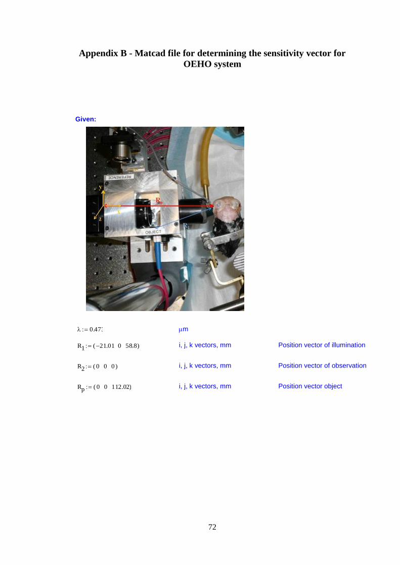
72
Appendix B - Matcad file for determining the sensitivity vector for
OEHO system
Given:
m
i, j, k vectors, mm Position vector of illumination
i, j, k vectors, mm Position vector of observation
i, j, k vectors, mm Position vector object
0.473
R1 21.01 0 58.8( )
R2 0 0 0( )
Rp 0 0 112.02( )

73
Solutions:
Unit vectors:
Unit vector for the direction of illumination
Unit vector form
Unit vector for the direction of observation
Unit vector form
Magnitudes
den_1 Rp0 0
R10 0
2Rp
0 1R1
0 1
2 Rp
0 2R1
0 2
2
den_1 57.217 mm
den_2 R20 0
Rp0 0
2R2
0 1Rp
0 1
2 R2
0 2Rp
0 2
2
den_2 112.02 mm
k1
Rp0 0
R10 0
den_1
Rp0 1
R10 1
den_1
Rp0 2
R10 2
den_1
k1 0.367 0 0.93( )
k1 0.367 i 0j 0.93k
k2
R20 0
Rp0 0
den_2
R20 1
Rp0 1
den_2
R20 2
Rp0 2
den_2
k2 0 0 1( )
k2 0 i 0 j 1 k
K1magnitude k10 0
2k1
0 1
2 k1
0 2
2 K1magnitude 1
K2magnitude k20 0
2k2
0 1
2 k2
0 2
2 K2magnitude 1

74
Vectors
Illumination vector
Observation vector
Given the three points, the illumination vectore came out to be, K1, while the observation vector, K2. For both cases, the magnitudes resulted in 0. Using this results, the sensitivity vector can be calculated follwoing the equation in the class notes.
Illumination vector
Observation vector
Sensitivity vector
Magnitude
k2
k 13.284
1
m
K1 k k1 K1 4.878 0 12.356( )
K1 4.878 i 0 j 12.356k1
m
K2 k k2 K2 0 0 13.284( )
K2 0 i 0 j 13.284 k1
m
Kill 4.878 0 12.356( )1
m
Kob 0 0 13.284( )1
m
Ktotal Kob0 0
Kill0 0
Kob0 1
Kill0 1
Kob0 2
Kill0 2
Ktotal 4.878 0 25.64( )1
m
Ktotal_mag Ktotal0 0
2Ktotal
0 1
2 Ktotal
0 2
2
Ktotal_mag 26.11
m

75
Unit vector
The procedure above calculated the sensitivity vector the the points specifed. The sensitivity
vector has units of 1/length, as K1 and K2. The magnitude was calculated to be 26.1 1/m. While the magnitude of its unit vector was 1, which is standard.
Ktotal_unit
Ktotal0 0
Ktotal_mag
Ktotal0 1
Ktotal_mag
Ktotal0 2
Ktotal_mag
Ktotal_unit 0.187 0 0.982( )
Kunit_mag Ktotal_unit0 0
2Ktotal_unit
0 1
2 Ktotal_unit
0 2
2
Kunit_mag 1