development of an en ergy system for a mo · pdf filefeup | resumo page 3 of ... professor...
TRANSCRIPT
DEVELOPMENT OF AN EN
RURAL VILLAGE WITHOU
Ricardo de Castro Amorim
Integrated Master in Mechanical Engineering
DEVELOPMENT OF AN ENERGY SYSTEM FOR A MOZAMBIQUE
RURAL VILLAGE WITHOUT ELECTRIC GRID ACCESS
Ricardo de Castro Amorim
DEMEGI
Integrated Master in Mechanical Engineering – Thermal Energy
MIEM
Porto, 2010
ZAMBIQUE
MIEM
Porto, 2010

DEVELOPMENT OF AN ENERGY SYSTEM FOR A MOZAMBIQUE RURAL VILLAGE WITHOUT ELECTRIC GRID ACCESS
FEUP | Abstract Page 2 of 110
Abstract
United Nations (UN) in 2000 created the Millennium Development Goals (MGD) with the
objective to reduce extreme poverty, reducing child mortality rates, fighting disease epidemics
and developing a global partnership for development. Engenharia para o Desenvolvimento e
Assistência Humanitária (EpDAH) is a non profitable and nongovernmental association which
has Autarkheia project, like other projects, that is based in the UN MDG. Autarkheia project
has the objective to identify critical factors and project engineer solutions to minimize or
eliminate these factors. The Autarkheia project is based in the multiplication and replication of
similar projects to other villages and enabling them to take responsibility from their own
development, minimizing extreme poverty and contributing access to education, health
services and decent living conditions. The village name is Malonguete and belongs to
Chicuacuala district, Gaza province of Mozambique. Using renewable energy technology it is
possible to provide villagers an energy system capable to produce water the entire year for the
population and capacitating the future village health center with a vaccine refrigerator that
operates with 2 to 8ºC temperature range for vaccine conservation.
To satisfy the water needs for 400 villagers, and based in a consumption profile for each
villager that is constant over the year the best studied system is a 320 Wp photovoltaic array
with a Grundfos SQFlex 2.5-2 helical rotor submersible pump. For the future health center it
was studied the water/lithium bromide absorption cycle and it was selected two refrigerators
with different vaccine volume capacity.

DEVELOPMENT OF AN ENERGY SYSTEM FOR A MOZAMBIQUE RURAL VILLAGE WITHOUT ELECTRIC GRID ACCESS
FEUP | Resumo Page 3 of 110
Resumo
As Nações Unidas no ano 2000 criaram os Objectivos de Desenvolvimento do Milénio (ODM)
com o objectivo de reduzir a pobreza extrema, reduzir a mortalidade infantil, combater
epidemias e desenvolver uma parceria global para o desenvolvimento. Engenharia para o
Desenvolvimento e Assistência Humanitária (EpDAH) é uma organização não governamental
sem fins lucrativos. O projecto Autarkheia, como outros projectos da associação, é baseado
nos ODM. Além do objectivo de desenvolver soluções de engenharia que sejam capazes de
suprimir as necessidades dos habitantes de uma aldeia também é necessário que esses
projectos sejam replicados e multiplicados por outras aldeias responsabilizando os habitantes
pelo seu próprio desenvolvimento. Assim o projecto contribui para o desenvolvimento,
reduzindo a pobreza extrema e contribuindo para um melhor acesso à educação, serviços de
saúde e condições de vida dignas. O nome da aldeia é Malonguete e situa-se na província de
Gaza, distrito de Chiqualaquala em Moçambique. Recorrendo a fontes de energia renovável é
possível capacitar a aldeia com um sistema de água que garanta o abastecimento de água a
400 habitantes e também capacitar o futuro centro de saúde de um refrigerador com a
capacidade de conservar vacinas que opera entre 2 e 8ºC.
Para satisfazer as necessidades de água a 400 habitantes e considerando que o consumo se
mantêm constante o melhor sistema estudado é um gerador fotovoltaico com 320 Wp e uma
bomba Grundfos SQFlex helical rotor 2.5-2. Foi estudado o ciclo frigorifico de absorção
brometo de lítio/água e seleccionou se dois refrigeradores com capacidades diferentes em
termos de volume para conservar vacinas.

DEVELOPMENT OF AN ENERGY SYSTEM FOR A MO
Preface
I’m volunteer since November of 2009 in the association
Assistência Humanitária (EPDAH). This dissertation was realized in collaboration with EpDAH
that has the mission to promote the human development through a prof
activity in the engineer domain. This dissertation is integrated in the Autarkheia project that
has the objective to identify critical factors and project engineer solutions to minimize or
eliminate these factors. The Autarkheia project
similar projects to other villages and
development, minimizing extreme poverty and contributing to access to education, health
services and decent living conditions
I want to show here my gratitude for the people that contributed for my experience in
Mozambique and helped me directly or indirectly realizing this dissertation
ERGY SYSTEM FOR A MOZAMBIQUE RURAL VILLAGE WITHOUT ELECTRIC GRID ACCESS
FEUP | Preface Page
I’m volunteer since November of 2009 in the association Engenharia para o Desenvolvimento e
This dissertation was realized in collaboration with EpDAH
that has the mission to promote the human development through a professional volunteer
activity in the engineer domain. This dissertation is integrated in the Autarkheia project that
has the objective to identify critical factors and project engineer solutions to minimize or
eliminate these factors. The Autarkheia project is based in the multiplication and replication of
similar projects to other villages and enabling them to take responsibility from their own
development, minimizing extreme poverty and contributing to access to education, health
conditions.
I want to show here my gratitude for the people that contributed for my experience in
Mozambique and helped me directly or indirectly realizing this dissertation
Anabela Seabra
António Amorim
Beatriz Barros
Professor Clito Afonso
Ernestina
Tiago Granja
GRID ACCESS
Page 4 of 110
Engenharia para o Desenvolvimento e
This dissertation was realized in collaboration with EpDAH
essional volunteer
activity in the engineer domain. This dissertation is integrated in the Autarkheia project that
has the objective to identify critical factors and project engineer solutions to minimize or
is based in the multiplication and replication of
own
development, minimizing extreme poverty and contributing to access to education, health
I want to show here my gratitude for the people that contributed for my experience in
Mozambique and helped me directly or indirectly realizing this dissertation
Anabela Seabra
António Amorim
Beatriz Barros
Clito Afonso
Ernestina Amorim
Tiago Granja

DEVELOPMENT OF AN ENERGY SYSTEM FOR A MOZAMBIQUE RURAL VILLAGE WITHOUT ELECTRIC GRID ACCESS
FEUP | Preface Page 5 of 110
Content
Abstract.......................................................................................................................................... 2
Resumo .......................................................................................................................................... 3
Preface ........................................................................................................................................... 4
Figures content list ........................................................................................................................ 8
Table content list ......................................................................................................................... 10
Nomenclature .............................................................................................................................. 12
1. Introduction ......................................................................................................................... 15
1.1 ONU Millennium Development Goals (MDG) .............................................................. 15
1.2 About Malonguete village ........................................................................................... 15
1.3 Systems used in developing countries to satisfy the water needs .............................. 17
1.4 Vaccine refrigerators used in developing countries .................................................... 18
1.5 Projects realized over the world – water systems ....................................................... 19
1.6 Sustainable development ............................................................................................ 19
2. Solar powered water pump systems ................................................................................... 21
2.1 Solar water pumps ....................................................................................................... 21
2.2 About water pumps ..................................................................................................... 22
2.3 Basic output parameters ............................................................................................. 25
2.4 Dimensionless pump performance .............................................................................. 26
2.5 The specific speed definition: Mixed and Axial Flow pumps ....................................... 26
2.6 Pump capacity and TDH ............................................................................................... 27
2.7 System head curve ....................................................................................................... 32
2.8 Pump H-Q curve ........................................................................................................... 33
2.9 Selecting a pump type and solar water pumps manufactures .................................... 34
2.10 Matching system components .................................................................................... 35
2.11 Electronic Unit Control ................................................................................................ 35
3. Photovoltaic Panels ............................................................................................................. 37
3.1 Semiconductors and J-n junctions ............................................................................... 37
3.2 The band model ........................................................................................................... 37
3.3 Semiconductors types ................................................................................................. 37
3.4 The p-n junctions ......................................................................................................... 38
3.5 The behaviour of solar cells – the I-V curve ................................................................ 39
3.6 Effect of temperature .................................................................................................. 40
3.7 Effect of parasitic resistance ........................................................................................ 41

DEVELOPMENT OF AN ENERGY SYSTEM FOR A MOZAMBIQUE RURAL VILLAGE WITHOUT ELECTRIC GRID ACCESS
FEUP | Preface Page 6 of 110
3.8 Photovoltaic modules in series and parallels .............................................................. 42
4. EES equations and results .................................................................................................... 43
4.1 Solar radiation on a sloped photovoltaic array ........................................................... 43
4.2 Photovoltaic I-V curve equations and results .............................................................. 44
4.3 Pump controller ........................................................................................................... 49
4.4 Maximum power point tracker .................................................................................... 50
4.5 Pump and water storage modulation – Grundfos SQFlex ........................................... 50
4.5.1 – Water Storage ................................................................................................... 52
4.6 Water pumping system results .................................................................................... 53
5. Pumping system results discussion ..................................................................................... 66
6. Pumping system components selection .............................................................................. 67
6.1 Village Water needs ..................................................................................................... 67
6.2 Components selection ................................................................................................. 67
7. Refrigeration system ............................................................................................................ 69
7.1 Working fluids .............................................................................................................. 69
7.1.1 Refrigerant designations ...................................................................................... 69
7.1.2 Absorption working fluids .................................................................................... 69
7.2 Differences between compression and absorption Ammonia/Water and
Water/Lithium Bromide cycles ................................................................................................ 70
8. Thermodynamic properties of absorption working fluids ................................................... 72
8.1 Mixtures diagrams ....................................................................................................... 72
8.1.1 Temperature-mass fraction diagram ................................................................... 72
8.1.2 Pressure-temperature diagram ........................................................................... 73
8.1.3 Enthalpy-mass fraction diagram .......................................................................... 73
9. Thermodynamic processes with mixtures ........................................................................... 75
9.1 Desorption ................................................................................................................... 76
9.2 Absorption ................................................................................................................... 77
9.3 Condensation and evaporation ................................................................................... 77
9.4 Compression ................................................................................................................ 78
9.5 Pumping ....................................................................................................................... 78
9.6 Throttling ..................................................................................................................... 78
9.7 Water/Lithium bromide cycle ...................................................................................... 78
9.8 Water/Lithium Bromide cycle limitations ................................................................... 80
9.9 Vacuum requirements ................................................................................................. 80

DEVELOPMENT OF AN ENERGY SYSTEM FOR A MOZAMBIQUE RURAL VILLAGE WITHOUT ELECTRIC GRID ACCESS
FEUP | Preface Page 7 of 110
9.10 Pressure drops ............................................................................................................. 80
9.11 Condenser and evaporator as heat exchangers .......................................................... 80
9.12 Lithium bromide absorption system analysis .............................................................. 82
9.12.1 Mass flow balances .............................................................................................. 82
9.12.2 Energy balances ................................................................................................... 83
9.13 Refrigeration capacity - Qe ........................................................................................... 84
9.13.1 Heat transfer by conduction through the walls ................................................... 85
9.13.2 Heat transfer by convection through the walls ................................................... 86
9.13.3 Heat transfer by radiation through the walls ...................................................... 87
9.14 Cycle thermodynamic states ....................................................................................... 88
10. Absorption System EES results ........................................................................................ 89
11. Absorption system results discussion .............................................................................. 98
12. Selecting Vaccine refrigerator ......................................................................................... 99
12.1 Product datasheet ..................................................................................................... 100
13. Conclusions .................................................................................................................... 102
14. References ..................................................................................................................... 103
Appendix A - Solar radiation ...................................................................................................... 105
A.1 - Definitions ..................................................................................................................... 105
A.1.1 - Direction of beam radiation ................................................................................... 105
A.2 - Ratio of beam radiation on tilted surface to that on horizontal surface ...................... 106
A.3 - Extraterrestrial radiation incident on a horizontal surface ........................................... 107
A.4 - Solar radiation data ....................................................................................................... 107
A.5 - Clearness index Kt .......................................................................................................... 107
A.6 - Diffuse component of monthly radiation ...................................................................... 108
A.7 - Estimation of hourly radiation from daily data ............................................................. 109
A.8 - Radiation incident on a tilted surface – Isotropic and anisotropic sky definition ......... 109

DEVELOPMENT OF AN ENERGY SYSTEM FOR A MOZAMBIQUE RURAL VILLAGE WITHOUT ELECTRIC GRID ACCESS
FEUP | Figures content list Page 8 of 110
Figures content list
Figure 1 – Mozambique map with province capitals ................................................................... 16
Figure 2 – Inhambane, Gaza and Maputo provinces. Chicualacuala district is the number 123
How can this project contribute to the development of this village? ......................................... 17
Figure 3 – Sustainable development diagram ............................................................................. 20
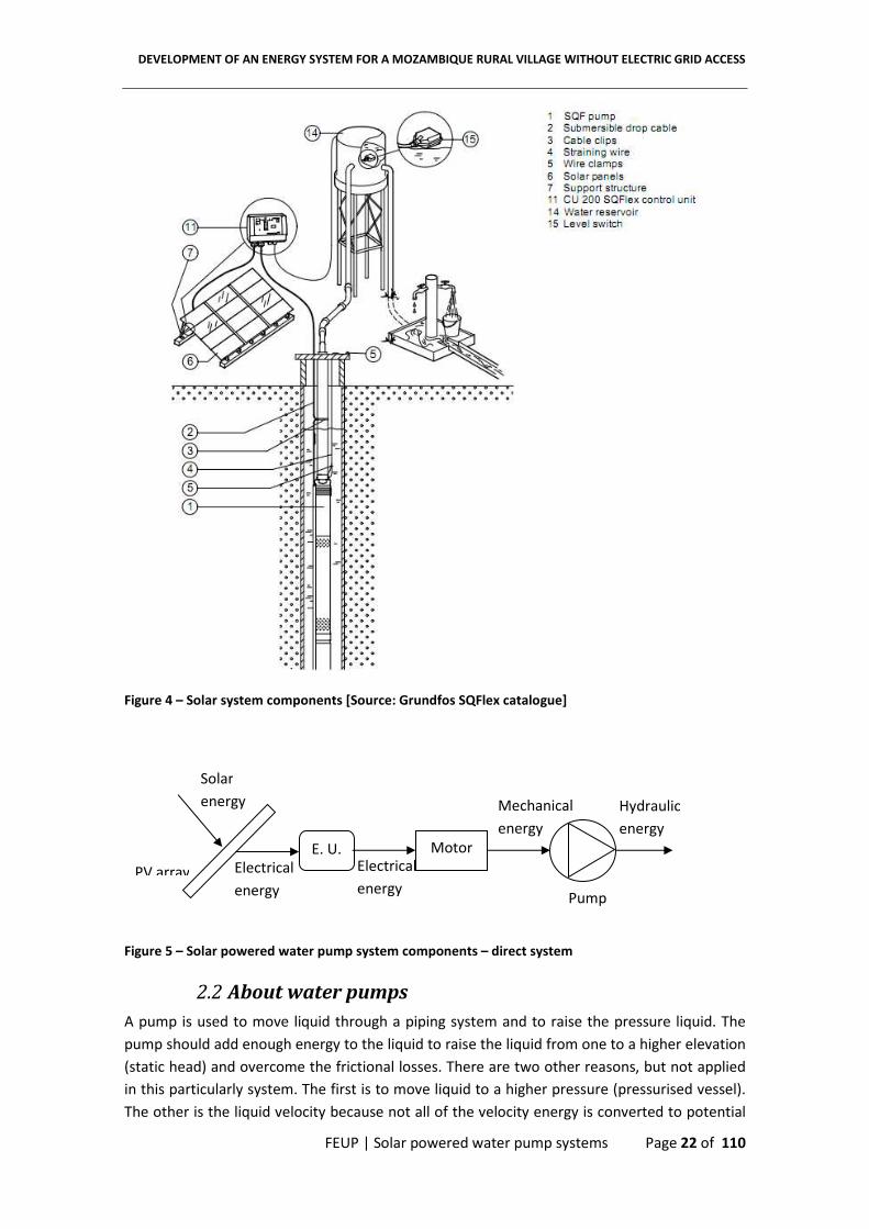
Figure 4 – Solar system components [source: Grundfos SQFlex catalogue] ............................... 22
Figure 5 – Solar powered water pump system components – direct system ............................. 22
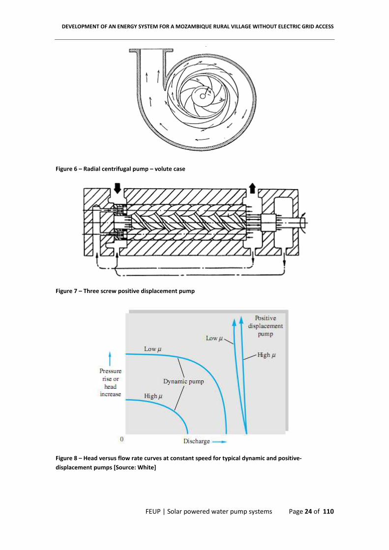
Figure 6 – Radial centrifugal pump – volute case ........................................................................ 24
Figure 7 – Three screw positive displacement pump .................................................................. 24
Figure 8 – Head versus flow rate curves at constant speed for typical dynamic and positive-
displacement pumps [Source: White] ......................................................................................... 24
Figure 9 – Vane design of dynamic pumps as a function of specific speed [Source: White] ...... 27
Figure 10 - Static head and pipe friction head ............................................................................. 28
Figure 11 – Darcy friction factor as a function of Reynolds and relative roughness (RR) drawn
using Eq. 6 .................................................................................................................................... 29
Figure 12 – Hf error by neglecting minor losses as function of Flow, Static head (H_est) and pipe
diameter for K=1,9 ....................................................................................................................... 30
Figure 13 - Hf error by neglecting minor losses as function of Flow, Static head (H_est) and pipe
diameter for K=4 .......................................................................................................................... 31
Figure 14 – Error in the annual predicted volume as a function of array area for the SQFlex HR
2.5-2 pump and K=4..................................................................................................................... 32
Figure 15 – System head-flow rate curve for 2 months of the year for D=38,1mm ................... 33
Figure 16 – Sunpump SCS 18-45 TDH, pump efficiency and motor power as a function of flow
rate and system head for the1st and 8th month of the year (pipe diameter D=1 ½ in and motor
voltage=45V) ................................................................................................................................ 34
Figure 17 – Grundfos SQF 5A-3 data [Source: Grundfos renewable energy pumps catalogue] . 35
Figure 18 – Brushed DC motor ........................................................ Erro! Marcador não definido.
Figure 19 – Motor speed (RPM), torque and efficiency as a function of current [Google books:
practical electrical motor handbook] .............................................. Erro! Marcador não definido.
Figure 20 - Speed (RPM), torque and efficiency as a function of motor voltage and current
[Source: Applied photovoltaics] ...................................................... Erro! Marcador não definido.
Figure 21 – Zenith angle (θz), slope (β), surface azimuth angle, and solar azimuth angle (ϒs) for a
tilted surface [Source: Duffie and Beckman] ............................................................................. 106
Figure 22 – Correlations of average diffuse fractions with average clearness index [Source:
Duffie] ........................................................................................................................................ 108
Figure 23 – Schematic of the energy bands for electrons in a solid [Source: Applied
photovoltaics] .............................................................................................................................. 37
Figure 24 – Application of a voltage to a p-n junction [Source: Applied photovoltaics] ............. 39
Figure 25 – The diode law for silicon –current as a function of voltage and temperature ......... 39
Figure 26 - Typical representation of an I-V curve showing maximum power and corresponding
maximum voltage and current and open circuit voltage (VOC) and short circuit current (Isc) ..... 40
Figure 27 – Effect of temperature on the I-V curve of a solar cell .............................................. 41
Figure 28 – Parasitic shunt and serie resistances in a solar cell circuit ....................................... 42

DEVELOPMENT OF AN ENERGY SYSTEM FOR A MOZAMBIQUE RURAL VILLAGE WITHOUT ELECTRIC GRID ACCESS
FEUP | Figures content list Page 9 of 110
Figure 29 – I-V curve for photovoltaic modules connected in various series and parallel
arrangements .............................................................................................................................. 42
Figure 30 – Example of photovoltaic array with two parallel strings of three in series
connection [Source: Sunpumps catalogue] ................................................................................. 45
Figure 31 - I-V curve for a single ISO160 PV panel....................................................................... 48
Figure 32 - I-V curve for 2 ISO160 PV panels connected in series ............................................... 48
Figure 33 – Vmp as function of GT. Equation and quadratic error ................................................. 50
Figure 34 – Mean monthly daily flow as a function of the year months for the 320Wp system
with SQF HR 2.5-2 pump (tilted array angle = 30º) ..................................................................... 54
Figure 35 - Mean monthly daily flow as a function of the year months for the 320Wp system
with SQF C 5A-3 pump (tilted array angle = 30º) ........................................................................ 55
Figure 36 - Annual predicted water volume as a function of array tilted angle and peak power
using SQF helical rotor (HR) 2.5-2 pump ..................................................................................... 56
Figure 37 - Annual predicted water volume as a function of array tilted angle and peak power
using SQF helical rotor (HR) 5A-3 pump ...................................................................................... 56
Figure 38 – SQF HR 2.5-2 pump efficiency as a function of pump output flow (discharge) and
total dynamic head ...................................................................................................................... 57
Figure 39- SQF C 5A-3 pump efficiency as a function of pump output flow (discharge) and total
dynamic head .............................................................................................................................. 58
Figure 40 – System efficiency (ISO160 + SQF HR 2.5-2) as a function of radiation incident in the
tilted array and array peak power for H_sta=7m ........................................................................ 60
Figure 41 - System efficiency (ISO160 + SQF C 5A-3) as a function of radiation incident in the
tilted array and array peak power for H_sta=7m ........................................................................ 60
Figure 42 - System efficiency (ISO160 + SQF HR 2.5-2) as a function of radiation incident in the
tilted array and array peak power for H_sta=11m ...................................................................... 61
Figure 43 - System efficiency (ISO160 + SQF C 5A-3) as a function of radiation incident in the
tilted array and array peak power for H_sta=11m ...................................................................... 61
Figure 44 – Water discharged cost as a function of array peak power and pump type, based in a
system lifetime = 10 years ........................................................................................................... 62
Figure 45 – Annual predicted discharged water volume as a function of array peak power and
pump type .................................................................................................................................... 62
Figure 46 – System relative components cost using a 320 Wp array .......................................... 63
Figure 47 - System relative components cost using a 800 Wp array ........................................... 64
Figure 48 – Absorption and vapor compression cycle differences [source: clito] ...................... 71
Figure 49 – Temperature mass fraction diagram – subcooled to superheated evolution .......... 73
Figure 50 – water/LiBr vapor pressure temperature diagram .................................................... 73
Figure 51 – Enthalpy mass fraction diagram for water/LiBr ........................................................ 74
Figure 52 - Enthalpy mass fraction diagram regions ................................................................... 74
Figure 53 – Two substance mixture with heat addition .............................................................. 75
Figure 54 – Desorption process scheme ...................................................................................... 76
Figure 55 – Absorption process scheme ...................................................................................... 77
Figure 56 - Water/lithium bromide cycle scheme ....................................................................... 79
Figure 57 – Refrigerator physical measures and surfaces ........................................................... 84
Figure 58 – Heat transfer resistance scheme for general refrigerator walls ............................... 85
Figure 59 - Heat transfer resistance scheme bottom refrigerator wall ....................................... 85

DEVELOPMENT OF AN ENERGY SYSTEM FOR A MOZAMBIQUE RURAL VILLAGE WITHOUT ELECTRIC GRID ACCESS
FEUP | Table content list Page 10 of 110
Figure 60 – Effect of solution heat exchanger on COP ................................................................ 91
Figure 61 – Refrigerator mean air temperature and evaporator heat rate as a function of
external temperature and considering that generator power is equal to 180W ........................ 92
Figure 62 – COP as a function of maximum and minimum LiBr mass fraction ........................... 93
Figure 63 – COP and refrigerator mean air temperature as a function of generator heat rate . 94
Figure 64 – COP and evaporator heat rate as a function of condenser length ........................... 95
Figure 65 – COP and heat transfer rate for generator, evaporator, and solution heat exchanger
as a function of pump flow .......................................................................................................... 95
Figure 66 – Absorption refrigerator COP and interior mean air temperature as a function of UAe
..................................................................................................................................................... 96
Table content list
Table 1 – Loss coefficient for several system components ......................................................... 30
Table 2 – Static head as a function for the 12 months ................................................................ 32
Table 3 – Global average monthly radiation taken over a period of 30 years in the
Maniquenique station [cuamba] and average day of the year [duffie] ...................................... 44
Table 4 - General constant values for photovoltaic I-V curve equations .................................... 44
Table 5 – Isofotón ISO160 catalogue data ................................................................................... 47
Table 6 - Cell temperature as a function of radiation considering Tamb=25ºC ............................. 49
Table 7 – Grundfos SQFlex pump data provided by the manufacturer ...................................... 50
Table 8 – Regression results for SQFlex 5A-3 pump .................................................................... 51
Table 9 - Regression results for SQFlex 2.5-2 pump .................................................................... 51
Table 10 – Grundfos SQFlex 5A-3 submersible pump data from Figure 14 ................................ 51
Table 11 – Grundfos SQFlex 2.5-2 (Helical rotor) submersible pump data ................................. 52
Table 12 – Solar water system configuration that were analysed .............................................. 53
Table 13 – Water volume in storage tanks as a function of tilted array angle, initial storage
volume and month for 320Wp with SQF HR 2.5-2 pump system ................................................ 53
Table 14 - Water volume in storage tanks as a function of tilted array angle, initial storage
volume and month for 320Wp with SQF C 5A-3 pump system ................................................... 54
Table 15 – Mean monthly daily flow for the system with SQF HR 2.5-2 pump and 320Wp ........ 55
Table 16 - Mean monthly daily flow for the system with SQF C 5A-3 pump and 320Wp ............ 55
Table 17 - Annual predicted water volume as a function of array tilted angle using SQF helical
rotor (HR) 2.5-2 pump and a 320 Wp array ................................................................................. 56
Table 18 - - Annual predicted water volume as a function of array tilted angle using SQF
centrifugal (C) 5A-3 pump and a 320 Wp array ............................................................................ 57
Table 19 – SQF HR 2.5-2 pump efficiency as a function of TDH and discharge ........................... 58
Table 20 - SQF C 5A-3 pump efficiency as a function of TDH and discharge ............................... 59
Table 21 - Annual predicted water volume and water cost as a function of array peak power
and pump type for a system lifetime = 10 years ......................................................................... 63
Table 22 – Total system cost, peak power cost and system relative components cost as a
function of array peak power (ISOfotón 160 peak power panels + Grundofos SQF pump +
Grundfos CU200 controller) ........................................................................................................ 64
Table 23 –System components unit price ................................................................................... 65
Table 24 – Refrigerant properties [Source: absorption] .............................................................. 70

DEVELOPMENT OF AN ENERGY SYSTEM FOR A MOZAMBIQUE RURAL VILLAGE WITHOUT ELECTRIC GRID ACCESS
FEUP | Table content list Page 11 of 110
Table 25 – Absorbent properties [Source: absorption] ............................................................... 70
Table 26 – Mixture properties [Source: absorption] ................................................................... 70
Table 27 – Coefficients and equation XPTO application domain ................................................ 76
Table 28 – Material properties that are possible to be used in the refrigerated ........................ 86
Table 29 – Base system operating points .................................................................................... 88
Table 30 – Refrigerator surfaces global heat transfer coefficient and respective resistances ... 89
Table 31 – Refrigerator exterior dimensions ............................................................................... 89
Table 32 – Exterior and interior surfaces areas ........................................................................... 89
Table 33 – Absorption system constants ..................................................................................... 90
Table 34 – Effect of solution heat exchanger on COP and refrigerator mean air temperature .. 91
Table 35 – Refrigerator COP, inside air and evaporator outlet temperatures as a function of
exterior temperature ................................................................................................................... 92
Table 36 – COP, condenser and absorber outlet temperatures and mean refrigerator air
temperature as a function of generator heat power .................................................................. 93
Table 37 – Condenser length effect on condenser outlet temperature, COP, evaporator heat
rate, refrigerator inside mean air temperature and evaporator outlet temperature ................ 94
Table 38 – COP, evaporator and generator heat transfer rates and evaporator and mean inside
refrigerator air temperature as a function of pump flow ........................................................... 96
Table 39 - Absorption refrigerator COP, evaporator heat rate, interior mean air temperature
and outlet evaporator temperature as a function of UAe ........................................................... 97
Table 40 – Zero Appliances GR265 G/E product performance information ............................. 100
Table 41 – Sibir V110GE product performance information according to EPI/PROC/5 ............ 100
Table 42 - Sibir V110GE product input/consumption information ........................................... 100
Table 43 - Zero Appliances GR265 G/E product specifications ................................................. 101
Table 44 - Sibir V110GE product specifications ......................................................................... 101

DEVELOPMENT OF AN ENERGY SYSTEM FOR A MOZAMBIQUE RURAL VILLAGE WITHOUT ELECTRIC GRID ACCESS
FEUP | Nomenclature Page 12 of 110
Nomenclature
Description Units Description Units
AM Air Mass �� Heat rate [W]
BHP Break Horse Power [W] ����� Radiation heat transfer [W]
���I;
SC
Short Circuit temperature
coefficient [1/ºC] �� � Absorber Heat Rate [W]
���V;
OC
Open Circuit temperature
coefficient [1/ºC] � � Condenser Heat Rate [W]
cp Specific heat at constant
pressure for vaccine [J/kgK] � � Evaporator Heat Rate [W]
CQ Pump Flow coefficient �� � Generator Heat Rate [W]
CQ Pump Power coefficient Refri.
Time Refrigeration time [s]
D Pump diameter [m] RPS Shaft speed [RPS]
� � Solution heat exchanger
efficiency RR Roughness Ratio
F Darcy friction factor rs Series resistance [Ω]
F Solution Circulating Ratio rs;ref Reference series resistance [Ω]
g Gravitation Acceleration [m2/s] rsh Shunt Resistance [Ω]
G Radiation incident on a
horizontal surface [W/m2] rt
Hourly and daily total
radiation on a horizontal
surface ratio
Gsc Solar constant [W/m2] T Absolute Temperature [K]
��,� Beam radiation [W/m2] Tair Ambient air temperature [ºC]
GT;ref Reference Radiation [W/m2] Tcel Cell temperature [ºC]
Hest Static Head [m] Tcel;ref Cell Reference Temperature [ºC]
Hf Friction head [m] Tcell Cell temperature [ºC]
� Monthly average radiation on
a horizontal surface [MJ/m2] TDH Total Dynamic Head [m]
�� Monthly average diffuse
radiation on a hor. surface [MJ/m2] ��� Outside air temperature [ºC]
DEVELOPMENT OF AN ENERGY SYSTEM FOR A MOZAMBIQUE RURAL VILLAGE WITHOUT ELECTRIC GRID ACCESS
FEUP | Nomenclature Page 13 of 110
�� Monthly average radiation in
a tilted surface [MJ/m2] Ur
Global heat transfer
coefficient [W/ºC]
I0
Extraterrestrial hourly
radiation on a horizontal
surface
[MJ/m2] V Velocity [m/s]
I0 Dark Saturation Current [A] v Specific volume [m3/kg]
��; �� Reference dark current [A] Ve Voltage [V]
Ib Beam radiation [MJ/m2] VI Pump energy consumption [MJ]
Id Diffuse radiation [MJ/m2] Vm Tank water volume in instant
m [m3]
Ie current [A] Vm-1
Tank water volume in instant
m-1 [m3]
IL Light Current [A] ��� Consumption flow [m3/day]
��;�� Reference Light current [A] ������� Mean daily flow in instant m [m3/day]
Imp Maximum Power Current [A] ������� Annual Volume [m3]
Imp
single
Maximum Power Current of a
single panel [A] ���!"
Mean daily flow in instant
m-1 [m3/day]
Isc Short Circuit Current [A] VOC Open Circuit Voltage [V]
ISC
single
Short Circuit Current of a
single panel [A]
VOC
single
Open Circuit Voltage of a
single panel [V]
IT Radiation incident on a tilted
surface [W/m2] W Refrigerator width [m]
�� Monthly average hourly
radiation [MJ/m2] WHP Water Horse Power [W]
K Boltzmann’s Constant [J/K] #� Compressor or pump power [W]
$� Average clearness index X Mass Fraction
$� Daily clearness index Z Height [m]
%� Hourly clearness index Greek
L Refrigerator length [m] &� Ground Reflectance
M Vaccine mass [kg] µ Dynamic viscosity [Pa.s]

DEVELOPMENT OF AN ENERGY SYSTEM FOR A MOZAMBIQUE RURAL VILLAGE WITHOUT ELECTRIC GRID ACCESS
FEUP | Page 14 of 110
m Air mass
'� Mass flow [kg/s] μI;SC Short Circuit temperature
coefficient [A/ºC]
n Average day of the year [day] μV;OC Open Circuit temperature
coefficient [V/ºC]
nmonth Number of days in month [day] β Tilted angle [º]
NOCT Normal Operating Cell
Temperature [ºC] δ Declination [º]
nrcel;s
Number of cells connected in
series Ε Surface Roughness [m]
nrpv
parallel
Number of PV panels
connected in paraller Θ Angle of incidence [º]
nrpv
serie
Number of PV panels
connected in series Θz Zenith angle [º]
Ns Specific speed ρ Specific mass [kg/m3]
Nu Nusselt number ϒ Surface azimuth angle [º]
P pressure [Pa] Φ Latitude [º]
Pmp Maximum Power Point [W] )*��* Pump efficiency
PVeff Photovoltaic panels efficiency ) Efficiency
PVpow
er
Photovoltaic panels power [W] + Hour angle [º]
Q Flow [m3/s] +s Sunset hour angle [º]
q Specific heat [J/kg]
qe Electron Charge [C]

DEVELOPMENT OF AN ENERGY SYSTEM FOR A MOZAMBIQUE RURAL VILLAGE WITHOUT ELECTRIC GRID ACCESS
FEUP | Introduction Page 15 of 110
1. Introduction
Collaborating with EpDAH that operates in Mozambique this project tries to apply engineering
knowledge with the objective to contribute to a better life for the population of a rural village
in Mozambique.
This project tries to give people enough water for consumption and possible to agriculture.
Developing the agriculture creates more food and develops the village. With money coming to
the village, villagers can buy other things that they need, for example, seeds, animals, upgrade
the water system. With water and a developed agriculture there is enough food for everyone
and with potable water disease decreases and people have a better quality of life.
Not only water contributes to a better quality life for the villagers. Give villagers health care is
very important and the association is considering building a health center. Some drugs and
vaccines need to be conserved at low temperatures (2ºC to 8ºC) and they are stored in
refrigerators.
The project, direct or indirectly, approach the following themes in the Autarkheia project:
• Energy
• Water
• Agriculture
• Health
• Economic activities
1.1 ONU Millennium Development Goals (MDG)
The millennium Development Goals are eight international development goals with 21 targets
and a series of measurable indicators for each target [38]. This project intervenes in Goal 6:
Combat HIV/AIDS, malaria and other diseases and in Goal 7: Ensure environmental
sustainability in the following targets:
• Target 6C: Have halted by 2015 and begun to reverse the incidence of malaria and
other major diseases
• Target 7C: Halve, by 2015, the proportion of people without sustainable access to safe
drinking water and basic sanitation
1.2 About Malonguete village
Malonguete village distance 80 km from the district capital city Chicualacuala (Figure 2)
located in Gaza province (Figure 1). There is only one road and is very precarious. Normally in
rainy days is almost impossible to circulate due to bad road state and surface rivers. So is
difficult to transport merchandise, people and animals. There for Malonguete is 3 or 4 hours
away from the district capital.
The people that live in the village are very poor and live from the local undeveloped
agriculture. There is an agriculture association since 2003. Since then they only afforded 3
cows. Their objective is to have one cow for each associate. There are about 400 villagers in

DEVELOPMENT OF AN ENERGY SYSTEM FOR A MOZAMBIQUE RURAL VILLAGE WITHOUT ELECTRIC GRID ACCESS
FEUP | Introduction Page 16 of 110
the village. It is very important to develop the village and create job opportunities so young
people don’t immigrate to other countries like South Africa.
The agriculture is for family sustain and depends on annual rainfall. Without enough water it’s
not possible to have a developed agriculture. There is a river which crosses the village named
“Chefu” (born in Zimbabwe). People build their houses along the river to have water near them
(maximum distance is 1 km). Some families go to the river every day and others only once per
weak because they have animals and wains to transport high volumes of water. Only a few
mouths of the year the river is at the surface (2 or 3 mouths). In the other mouths they have to
dig to have access to water. The water is for consumption because they don’t have the habit to
irrigate the crops. The animals they have are not for consumption. Animals are used as a bank
account. For example, when someone gets ill they sell an animal to have money for the
treatment. The nearest health center distance 12 km from the village and there is only
transport two times a week (Wednesday and Friday). Usually people use bikes or their own
feet.
The village have a well that needs maintenance. Today nobody uses that well. It was built in
2007 and belongs to the villagers. Villagers said that this well, since it was built, never run dry.
They stop using the well because the wood seal that closes the tank from atmosphere was
taken by the river.
Figure 1 – Mozambique map with province capitals

DEVELOPMENT OF AN ENERGY SYSTEM FOR A MOZAMBIQUE RURAL VILLAGE WITHOUT ELECTRIC GRID ACCESS
FEUP | Introduction Page 17 of 110
Figure 2 – Inhambane, Gaza and Maputo provinces. Chicualacuala district is the number 123
1.3 Systems used in developing countries to satisfy the
water needs
Actually there are two mature water systems that are widely applied in developing countries
with villages without grid power. The most reliable (and expensive) is the solar water pumps
system. Experience of operating PV pumps has shown that due to their simplicity, high
reliability and the stand-alone operation these systems are appropriate for remote rural areas
[I. Odeh et. al, 2005]. On the other hand it is used diesel powered pumps. Diesel pumps are
characterized by a lower first cost but a very high running and maintenance costs. Solar is the
opposite. Solar pumps sometimes run for years without anyone touching them [Self, 2008].
Sometimes it’s not the cost of diesel maintenance that cares but the time to repair the
malfunction. In a village were crops depend on water one or four weeks without water could
mean the crops end. So it is important to achieve a compromise between first cost, running
cost and reliability. Another problem for diesel pumps is the escalating fuel prices and fuel
shortages [Self, 2008].
Diesel pumps required sometimes skilled labour hand. Solar powered pumps normally are
simpler systems and require unskilled labour to keep them running. The most frequency
maintenance in solar systems is cleaning the dust from PV array every 2-4 weeks [Self, 2008].
In some cases it is almost impossible to have a solar powered pump. But this is the case were
fuel is very cheap and the system power is very high. I. Odeh et. al (2005) showed that PV
water pumping systems have shown better economic viability than diesel water pumping

DEVELOPMENT OF AN ENERGY SYSTEM FOR A MOZAMBIQUE RURAL VILLAGE WITHOUT ELECTRIC GRID ACCESS
FEUP | Introduction Page 18 of 110
systems for equivalent hydraulic energy capacities of up to 8000 m4/day, 4100 m4/day and
2600 m4/day depending on the interest rate. Hydraulic energy is defined by equation 1.
�-./01234 565/7- 8 �. �� Eq. 1
Wind powered pumps have shown a reliable potential in some remote areas [Vick, 1996]. A
mechanical wind pump, like the name suggests, transforms wind energy in mechanical energy.
Electric-wind water pump produces electric energy from wind energy. The mechanical wind
powered pump was applied many years ago. Today is more frequent to use electric-wind or
solar water pumps. Both needs some local studies to predict the energy output from the
system. If the collected data over a year isn’t accurate the wind-electric system could be a
failure because the power output varies with the cubic of wind velocity. In this area
(Chicualacuala) is very difficult to obtain technical data. They only register the precipitation in
the district capital. Depending on wind and radiation conditions at the local the wind-electric
generator could produce much more energy if the local has high mean wind speeds. Like in the
diesel systems is hard to tell witch system is better to apply because there is no data about
weather conditions (wind and radiation on site).
Considering the solar radiation data in the Maniquenique station, the only system that can
satisfy the village needs of water, in a simple and reliable way is the solar powered pumps.
There is another possibility: a hybrid system that operates most of the time using solar energy
and in case of failure the backup system activates (Diesel or Otto cycle). Failure here means
system malfunction or insufficient energy production (several rainy days). The backup system
could be a gasoline or diesel engine.
1.4 Vaccine refrigerators used in developing countries
Refrigeration systems are divided in three categories: 1) electric operated; 2) thermal
operated; 3) hybrid systems [Afonso, 2007]. Electric grid access is limited outside the country
coastal cities and the alternatives normally are vapour compression cycle powered with
photovoltaic technology or thermal operated with and absorption cycle by burning gas as a
heat source or other heat source.
Photovoltaic refrigerators are powered by sun and at night or when the sun irradiation is low
the refrigerator is running due to the application of deep cycle batteries that stores electric
energy. As an electric energy source it could be used a diesel generator our wind but for the
reasons pointed above they are not commonly used.
Thermal operated refrigerators use a heat source to produce a cold effect and this is achieved
using an absorption cycle. Common refrigerators use an ammonia/water or water/lithium
bromide fluids (refrigeration fluid/absorber) and as a heat source. These refrigerators are
interesting because they have no moving parts and use gas or propane as their primary source
of energy. Also these refrigerators could use a thermal solar collector to power the generator.

DEVELOPMENT OF AN ENERGY SYSTEM FOR A MOZAMBIQUE RURAL VILLAGE WITHOUT ELECTRIC GRID ACCESS
FEUP | Introduction Page 19 of 110
To select the right category several parameters should be analysed, for example:
• Initial system cost
• Maintenance and operation cost
• Fuel transport and shortages
• System reliability
1.5 Projects realized over the world – water systems
Solar Energy For Africa Ltd (SEFA Ltd) is a private company specialized in photovoltaic business
with projects particularly in Uganda and in the East African region in general. From the list of
their projects two of them are very similar to the project realized in this dissertation:
• Solar water pumping system at Moroto Municipality - A Grundfos SP 3A 10/140 volts is
powered by 32 photovoltaic panels each one with a 50 watt peak that pumps 50 cubic
meters per day of water at a head of 60 meters that is stored in a tank.
• Solar water pumping system at Usuk Health center – Funded by the NGO of Soroti
Catholic Diocese Development Organization (SOCADIDO) SEFA installed a SQFlex 2.5-2
system powered by 14 photovoltaic panels each one with 50 watt peak pumping 15
cubic meters of water per day at a head of 40 meters from the borehold to the tank.
NAPS System group is located in Finland and since 1981 delivered solar electric systems to
more than 50 countries all over the world, one of them is the water supply in Yemen. The
system was designed for a high mountain application in the west coastal area of Yemen and is
powered by 24 photovoltaic panels producing 1200 peak watts to pump 8000 to 9000 liters
per day (very high heads).
1.6 Sustainable development
Sustainable development has three pillars: 1) economic; 2) social; 3) environmental. Diesel
motors pollute air by emitting CO2 and other polluting gases. However, it is in the economic
side. Solar powered water pumps are in the environmental side and runs away from the
economical side. Both of them have positive and negative impacts in society. The ideal energy
production technology is the balance between economy, society and environment.

DEVELOPMENT OF AN ENERGY SYSTEM FOR A MOZAMBIQUE RURAL VILLAGE WITHOUT ELECTRIC GRID ACCESS
FEUP | Introduction Page 20 of 110
Figure 3 – Sustainable development diagram

DEVELOPMENT OF AN ENERGY SYSTEM FOR A MOZAMBIQUE RURAL VILLAGE WITHOUT ELECTRIC GRID ACCESS
FEUP | Solar powered water pump systems Page 21 of 110
2. Solar powered water pump systems
The simplest Solar Water Pump (SWP) consist in a PV array, power controller, a water pump
operated by a DC brushless motor and a storage tank (direct-coupled system – see figure 4 and
Figure 5). There is another system that needs a DC/AC inverter if the electric motor uses AC
current. The system gets more expensive with the addition of batteries (battery-coupled
system) and possible less reliable. If the system is not carefully dimensioned the overall system
efficiency is reduced with batteries because batteries dictate the operating voltage and not the
PV panels [Buschermohle,]. This reduced efficiency could be minimized if a proper controller is
selected to boost the battery voltage supply to the water pump. Using batteries increase
initial, operating and maintenance costs. In this particular case there is no need to install
batteries because solar energy is stored in water tanks in the form of potential energy. Figure 4
exemplifies a direct couple system with a storage tank.
Another problem of battery-coupled system is the battery life time. With high temperatures
the battery life time becomes smaller resulting in a more frequency battery replacement.
Another issue is an ambient problem. What services Mozambique provide to recycle old
batteries replacing the old ones with new batteries? Normally batteries sold are car battery
and they are not suited to PV systems. In rural areas batteries should be avoided if possible.
Batteries could be used if it is need to store electric energy and use the electric energy when
the generator can’t produce energy providing the system autonomy for several days
depending on consumption. Batteries probably are the weakest element in a PV system and
needs control system to avoid overcharging and over discharging. Huacuz, Jorge M. concluded
that human interaction with batteries and batteries control has a big impact in batteries life
time.
2.1 Solar water pumps
Solar water pumps are designed to use solar power efficiently. Electric motors that are coupled
to the pump could use AC or DC current. Solar arrays produce DC current and to transform in
AC current it is necessary to install additional equipment to transform DC to AC current (DC/AC
inverter). Using this equipment generally reduces system efficiency but induction motors are
reliable and maintenance free operation and less expensive. DC motors, except brushless
motors, need frequent maintenance because of the sliding brush contacts. Brushless motors
are available for applications that require low power which are suitable to solar water systems.
The only problem of using brushless motors is there high cost. Nowadays some manufactures
produce submersible pumps with brushless motors.
DEVELOPMENT OF AN ENERGY SYSTEM FOR A MOZAMBIQUE RURAL VILLAGE WITHOUT ELECTRIC GRID ACCESS
FEUP | Solar powered water pump systems Page 22 of 110
Figure 5 – Solar powered water pump system components – direct system
2.2 About water pumps
A pump is used to move liquid through a piping system and to raise the pressure liquid. The
pump should add enough energy to the liquid to raise the liquid from one to a higher elevation
(static head) and overcome the frictional losses. There are two other reasons, but not applied
in this particularly system. The first is to move liquid to a higher pressure (pressurised vessel).
The other is the liquid velocity because not all of the velocity energy is converted to potential
E. U. Motor Electrical
energy
Solar
energy
Electrical
energy
Mechanical
energy
Hydraulic
energy
PV array
Pump
Figure 4 – Solar system components [Source: Grundfos SQFlex catalogue]

DEVELOPMENT OF AN ENERGY SYSTEM FOR A MOZAMBIQUE RURAL VILLAGE WITHOUT ELECTRIC GRID ACCESS
FEUP | Solar powered water pump systems Page 23 of 110
or pressure energy. The last one should take importance in calculations when the pressure is
measured in a point where velocity isn’t zero.
Pumps transform mechanical energy (torque, horsepower) to raise liquids pressure. To do this
transformation there are two principals which results in different types of pumps. Positive
displacement pumps increases liquid energy periodically by applying force to one or more
moveable volumes. A three screw PDP is shown in Figure 6. Listed below are some positive
displacement pump types:
• Reciprocating
1. Piston or plunger
2. Diaphragm
• Rotary
1. Single rotor
I. Sliding vane
I. Flexible tube or lining
II. Screw
III. Peristaltic
2. Multiple rotors
I. Gear
II. Lobe
III. Screw
IV. Circumferential piston
Dynamic pumps increase liquid velocity by means of fast moving blades or vanes and when the
velocity is reduced the liquid pressure increase by exiting into a diffuser section. Water enters
the impeller at the center and flows radially outward and is discharged from the circumference
into the case. In the impeller the fluid gains velocity and pressure at the same time. The
doughnut-shaped diffuser section of the casing decelerates the flow and further increases the
pressure. See Figure 6 to better understand. The diffuser may be vaneless as in Figure 6 or
fitted with fixed vanes to help guide the flow toward the exit. There is no closed volume and
the liquid energy is continuously increased. The discharge is smooth and has less vibration
problems than PD pumps requiring minor foundations. Listed below are some kinetic type
pumps:
• Centrifugal
1. Radial exit flow
2. Axial flow
3. Mixed flow (between radial and axial)
• Special designs
DEVELOPMENT OF AN ENERGY SYSTEM FOR A MOZAMBIQUE RURAL VILLAGE WITHOUT ELECTRIC GRID ACCESS
FEUP | Solar powered water pump systems Page 24 of 110
Figure 6 – Radial centrifugal pump – volute case
Figure 7 – Three screw positive displacement pump
Figure 8 – Head versus flow rate curves at constant speed for typical dynamic and positive-
displacement pumps [Source: White]

DEVELOPMENT OF AN ENERGY SYSTEM FOR A MOZAMBIQUE RURAL VILLAGE WITHOUT ELECTRIC GRID ACCESS
FEUP | Solar powered water pump systems Page 25 of 110
For this project the working fluid is water and only the first two items in the following list are
important. The difference between the two pump types behaviour to the dynamic viscosity is
shown in Figure 8. To select a PD pump instead of a centrifugal pump type the following
applications key criteria must be met:
• High pressure
• Low flow
• High viscosity
• High efficiency
• Low velocity
• Low shear
• Self priming
The first two items in the list should be considered in more attention. It is also possible to find
a centrifugal pump that produces very high pressures. And smaller centrifugal pumps are able
to deliver small amounts of water. If the application needs very high pressure and demands a
low flow then only the PD pumps can satisfy both conditions. Other listed items are important
if the fluid wasn’t water.
2.3 Basic output parameters
Assuming steady flow, neglecting viscous work, heat transfer and incompressible flow the
pump head is equal to:
� 8 : ;& · 7 = �>2 · 7 = @A
>= : ;& · 7 = �>
2 · 7 = @A"
Eq. 2
The velocity in the inlet and exit are almost the same and the difference between z2 and z1 is
minimum and the net head is approximately equal to:
∆� C ∆;& · 7 Eq. 3
Water horse power (WHP) or hydraulic power is the power delivered by the pump to the fluid
for a given specific gravity, flow and head.
#�; 8 & · 7 · � · � Eq. 4
The power required to power the pump is called break horsepower (BHP) and is equal to the
torque (T) developed by the motor and the shaft angular velocity (+).
D�; 8 + · � Eq. 5
Pump effectiveness is defined by the ratio between the hydraulic power and the break
horsepower delivered by the motor.
) 8 #�;D�; Eq. 6
DEVELOPMENT OF AN ENERGY SYSTEM FOR A MOZAMBIQUE RURAL VILLAGE WITHOUT ELECTRIC GRID ACCESS
FEUP | Solar powered water pump systems Page 26 of 110
)�E�E� 8 D�;�254F/34 GHI5/ 36G1F Eq. 7
)J��_*��* 8 #�;�254F/34 GHI5/ 36G1F Eq. 8
Submersible pumps manufactures assemble the pump and the motor in the same case that is
sealed to avoid water inlet to electronic components. The electric power input required by the
motor and the water horse power produced by the pump are normal data displayed in their
catalogues.
2.4 Dimensionless pump performance
The output variables head and break horsepower should be dependent upon discharge (Q),
rotational shaft speed and impeller diameter. Other possible parameters are the fluid viscosity
µ, density ρ and surface roughness ε.
7 · �L;M> · N> 8 g" : QRPS · DU , ρnD>µ , YDA
Eq. 9
D�;& · L;MU · NZ 8 g> : QRPS · DU , ρnD>µ , YDA
Eq. 10
The quantities ρnD>/µ and Y/D are the Reynolds number and roughness ratio (RR),
respectively. The pump dimensionless parameters, capacity, head and power coefficient,
respectively, are equal to:
�\ 8 QRPS · D> Eq. 11
�] 8 g · HRPS> · D> Eq. 12
�_ 8 BHPρ · RPSU · DZ Eq. 13
The pump efficiency is already dimensionless and is related to the other three dimensionless
parameters:
) 8 �\ · �]�_ Eq. 14
2.5 The specific speed definition: Mixed and Axial Flow
pumps
Specific speed is a dimensional number that it is used to select the best size and shape
(centrifugal, mixed or axial) for the pump. To calculate Ns it is necessary to know the head and
discharge at BEP (best efficiency point) and pump (or motor) speed.
DEVELOPMENT OF AN ENERGY SYSTEM FOR A MOZAMBIQUE RURAL VILLAGE WITHOUT ELECTRIC GRID ACCESS
FEUP | Solar powered water pump systems Page 27 of 110
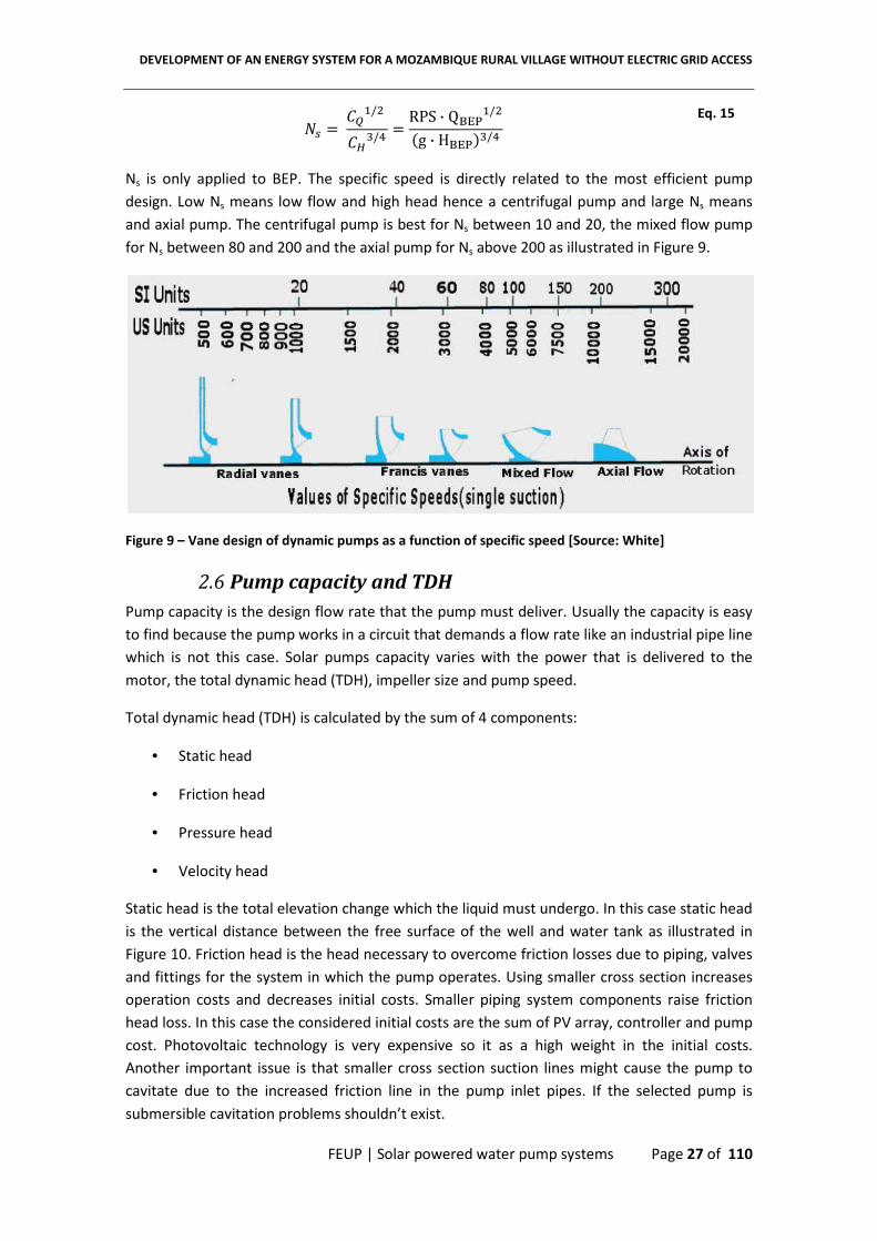
aJ 8 �\"/> �]U/b 8 RPS · Qcde"/>
fg · HcdegU/b Eq. 15
Ns is only applied to BEP. The specific speed is directly related to the most efficient pump
design. Low Ns means low flow and high head hence a centrifugal pump and large Ns means
and axial pump. The centrifugal pump is best for Ns between 10 and 20, the mixed flow pump
for Ns between 80 and 200 and the axial pump for Ns above 200 as illustrated in Figure 9.
Figure 9 – Vane design of dynamic pumps as a function of specific speed [Source: White]
2.6 Pump capacity and TDH
Pump capacity is the design flow rate that the pump must deliver. Usually the capacity is easy
to find because the pump works in a circuit that demands a flow rate like an industrial pipe line
which is not this case. Solar pumps capacity varies with the power that is delivered to the
motor, the total dynamic head (TDH), impeller size and pump speed.
Total dynamic head (TDH) is calculated by the sum of 4 components:
• Static head
• Friction head
• Pressure head
• Velocity head
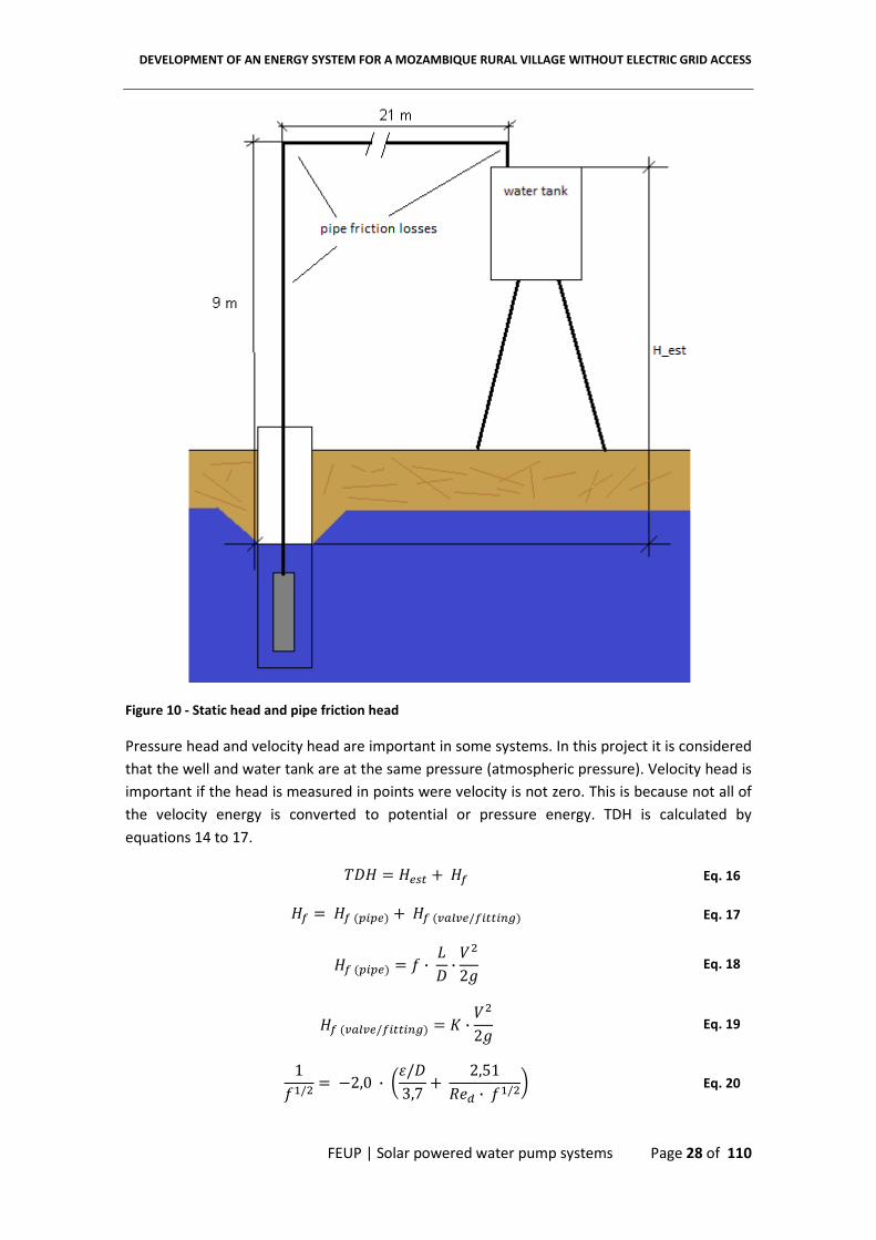
Static head is the total elevation change which the liquid must undergo. In this case static head
is the vertical distance between the free surface of the well and water tank as illustrated in
Figure 10. Friction head is the head necessary to overcome friction losses due to piping, valves
and fittings for the system in which the pump operates. Using smaller cross section increases
operation costs and decreases initial costs. Smaller piping system components raise friction
head loss. In this case the considered initial costs are the sum of PV array, controller and pump
cost. Photovoltaic technology is very expensive so it as a high weight in the initial costs.
Another important issue is that smaller cross section suction lines might cause the pump to
cavitate due to the increased friction line in the pump inlet pipes. If the selected pump is
submersible cavitation problems shouldn’t exist.
DEVELOPMENT OF AN ENERGY SYSTEM FOR A MOZAMBIQUE RURAL VILLAGE WITHOUT ELECTRIC GRID ACCESS
FEUP | Solar powered water pump systems Page 28 of 110
Figure 10 - Static head and pipe friction head
Pressure head and velocity head are important in some systems. In this project it is considered
that the well and water tank are at the same pressure (atmospheric pressure). Velocity head is
important if the head is measured in points were velocity is not zero. This is because not all of
the velocity energy is converted to potential or pressure energy. TDH is calculated by
equations 14 to 17.
�N� 8 �J� h �� Eq. 16
�� 8 �� f*i*g h �� fj� j/�i��i��g Eq. 17
�� f*i*g 8 k · lN · �>27 Eq. 18
�� fj� j/�i��i��g 8 $ · �>27 Eq. 19
1k"/> 8 =2,0 · o�/N3,7 h 2,51L5� · k"/>s Eq. 20

DEVELOPMENT OF AN ENERGY SYSTEM FOR A MOZAMBIQUE RURAL VILLAGE WITHOUT ELECTRIC GRID ACCESS
FEUP | Solar powered water pump systems Page 29 of 110
The program selected to solve the equations (EES) has built in functions that are suited to be
solved using computer calculations. The Darcy friction factor “f” is calculated using the
Churchill correlation (Eq. 21). The function input variables are the Reynolds number (Eq. 22)
and relative roughness (Eq. 23). The Churchill relation provides a smooth transition between
laminar and turbulent flow regimes as shown in Figure 11. This eliminates the use of a function
that determines if the flow is laminar or turbulent and the use of two equations for each fluid
regime.
The value in Figure 11 for relative roughness was calculated for D=11/2 (38,1 mm) and ε =
0,0015mm (plastic pipe roughness) [White, 2003].
Eq. 21
L5� 8 & · � · Nμ Eq. 22
LL 8 �N Eq. 23
Figure 11 – Darcy friction factor as a function of Reynolds and relative roughness (RR) drawn using Eq.
21
Hf also depends from local losses, i.e., valves, fittings, sudden expansion or contraction, bends,
inlets and outlets. These losses are measured experimentally and correlated with flow
parameters. The loss coefficient K is given by Eq. 24.
f = 8 · 8
Re
12
+ 2,457 · ln1
7
Re
0,9
+ 0,27 · rough
16
+ 37530
Re
16 – 1,5
1
12
500 1000 10000 1000000,01
0,03
0,05
0,07
0,09
0,11
0,13
Re
f
Laminar
Turbulent
Transition
RR=0,00005
DEVELOPMENT OF AN ENERGY SYSTEM FOR A MOZAMBIQUE RURAL VILLAGE WITHOUT ELECTRIC GRID ACCESS
FEUP | Solar powered water pump systems Page 30 of 110
$ 8 ∆;12 &�> Eq. 24
The value K can be obtained from manufactures catalogues or consulting tables in the
bibliography. These additional losses are also called minor losses [White, 2003]. There is an
error associated by not taking into account these minor losses. It is difficult to know all the
local losses, but as exampled in Table 1 it is considered that the total loss coefficient K is equal
to 4. The considered pipe length is 30 meters as shown in figure 10.
Table 1 – Loss coefficient for several system components
Description K
Pump entrance 0,5
90º regular elbow (screwed) 2x1,25
Tank discharge 1
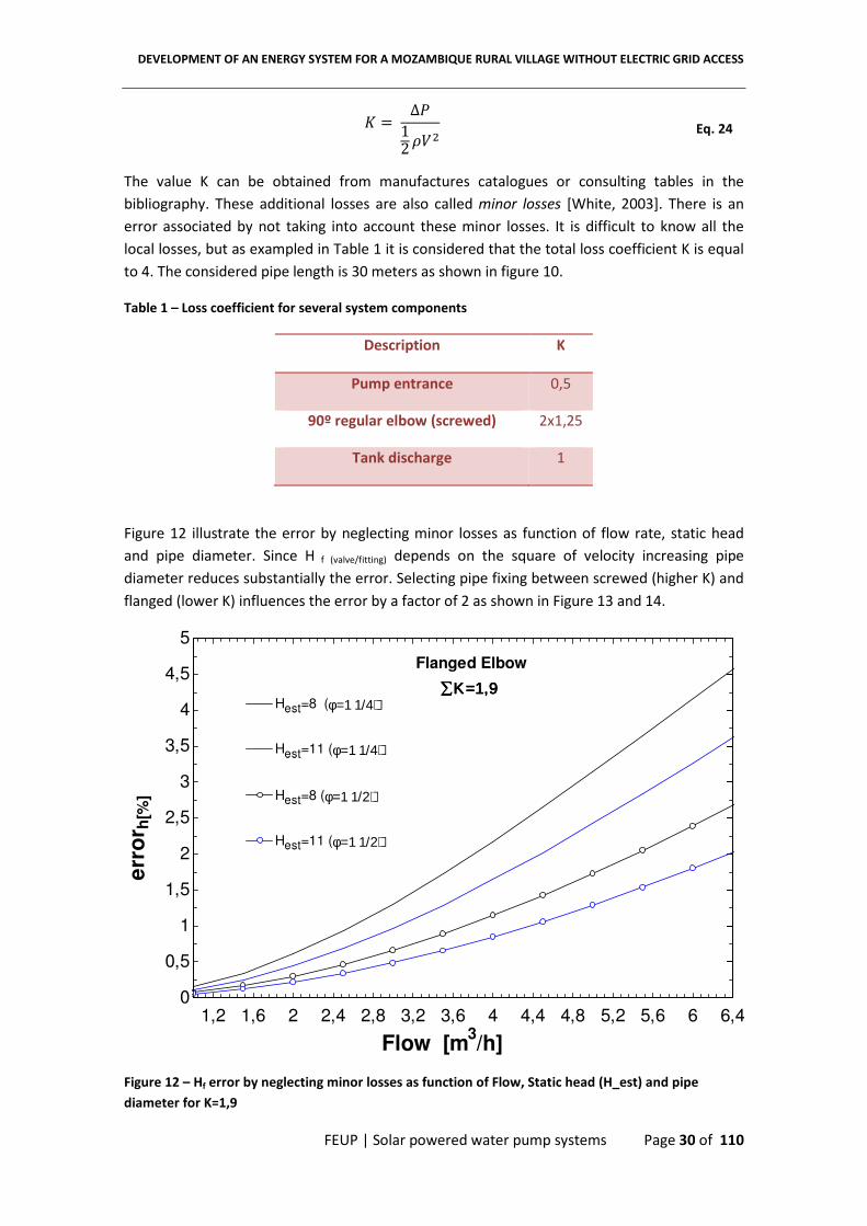
Figure 12 illustrate the error by neglecting minor losses as function of flow rate, static head
and pipe diameter. Since H f (valve/fitting) depends on the square of velocity increasing pipe
diameter reduces substantially the error. Selecting pipe fixing between screwed (higher K) and
flanged (lower K) influences the error by a factor of 2 as shown in Figure 13 and 14.
Figure 12 – Hf error by neglecting minor losses as function of Flow, Static head (H_est) and pipe
diameter for K=1,9
1,2 1,6 2 2,4 2,8 3,2 3,6 4 4,4 4,8 5,2 5,6 6 6,40
0,5
1
1,5
2
2,5
3
3,5
4
4,5
5
Flow [m3/h]
err
or h
[%]
Hest=8 (φ=1 1/4)Hest=8 (φ=1 1/4)
Hest=11 (φ=1 1/4)Hest=11 (φ=1 1/4)
Hest=8 (φ=1 1/2)Hest=8 (φ=1 1/2)
Hest=11 (φ=1 1/2)Hest=11 (φ=1 1/2)
Flanged Elbow
∑∑∑∑ΚΚΚΚ====1111,,,,9999

DEVELOPMENT OF AN ENERGY SYSTEM FOR A MOZAMBIQUE RURAL VILLAGE WITHOUT ELECTRIC GRID ACCESS
FEUP | Solar powered water pump systems Page 31 of 110
Figure 13 - Hf error by neglecting minor losses as function of Flow, Static head (H_est) and pipe
diameter for K=4
The error considering ΣK=1,9 or ΣK=4 compared to the TDH considering ΣK=0 is calculated by
equation 25.
5//H/t 8 �N� = �N�uv��N� Eq. 25
In Figure 14 the Hf error, by neglecting the minor losses, as minimum impact in the annual
water volume predicted, for the SQF 2.5-2 system, and varies linearly with the array area.
Otherwise indicated the loss coefficient will have the value of 4. It’s hard to predict all the
minor losses due to a several reasons (from the most to the less influent):
• Connection type – flanged or screwed
• Tube roughness can vary from 0.0015 to 0.007 mm (ε/D ratio)
• Elbow radius or R/D ratio
The annual predicted volume of water error is defined as
5//H/t 8 ������� = ������� ;uv�������� Eq. 26
1,2 1,6 2 2,4 2,8 3,2 3,6 4 4,4 4,8 5,2 5,6 6 6,40
1
2
3
4
5
6
7
8
9
Flow [m3/h]
err
or h
[%]
Hest=8 (φ=1 1/4)Hest=8 (φ=1 1/4)
Hest=11 (φ=1 1/4)Hest=11 (φ=1 1/4)
Hest=8 (φ=1 1/2)Hest=8 (φ=1 1/2)
Hest=11 (φ=1 1/2)Hest=11 (φ=1 1/2)
Screwed Elbow
∑∑∑∑ΚΚΚΚ====4444
DEVELOPMENT OF AN ENERGY SYSTEM FOR A MOZAMBIQUE RURAL VILLAGE WITHOUT ELECTRIC GRID ACCESS
FEUP | Solar powered water pump systems Page 32 of 110
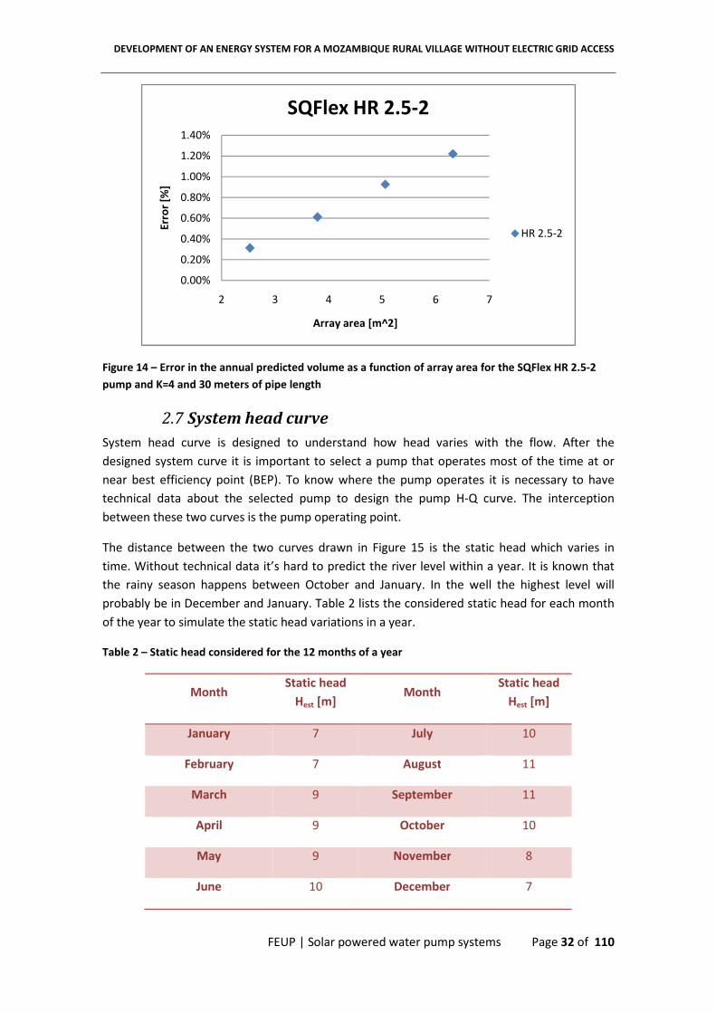
Figure 14 – Error in the annual predicted volume as a function of array area for the SQFlex HR 2.5-2
pump and K=4 and 30 meters of pipe length
2.7 System head curve
System head curve is designed to understand how head varies with the flow. After the
designed system curve it is important to select a pump that operates most of the time at or
near best efficiency point (BEP). To know where the pump operates it is necessary to have
technical data about the selected pump to design the pump H-Q curve. The interception
between these two curves is the pump operating point.
The distance between the two curves drawn in Figure 15 is the static head which varies in
time. Without technical data it’s hard to predict the river level within a year. It is known that
the rainy season happens between October and January. In the well the highest level will
probably be in December and January. Table 2 lists the considered static head for each month
of the year to simulate the static head variations in a year.
Table 2 – Static head considered for the 12 months of a year
Month Static head
Hest [m] Month
Static head
Hest [m]
January 7 July 10
February 7 August 11
March 9 September 11
April 9 October 10
May 9 November 8
June 10 December 7
0.00%
0.20%
0.40%
0.60%
0.80%
1.00%
1.20%
1.40%
2 3 4 5 6 7
Err
or
[%]
Array area [m^2]
SQFlex HR 2.5-2
HR 2.5-2

DEVELOPMENT OF AN ENERGY SYSTEM FOR A MOZAMBIQUE RURAL VILLAGE WITHOUT ELECTRIC GRID ACCESS
FEUP | Solar powered water pump systems Page 33 of 110
Figure 15 – System head-flow rate curve for 2 months of the year for D=38,1mm
The system head flow is drawn by varying the flow rate and from equations 16 to 20 the TDH is
calculated and plot against the flow rate. The curve slope depends from flow rate, pipe
diameter and minor losses.
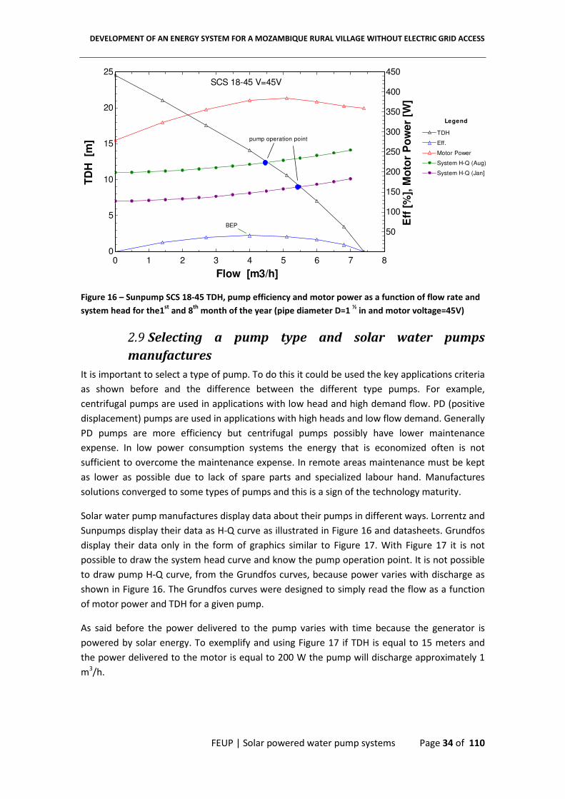
2.8 Pump H-Q curve
The flow delivered by the pump varies with the head. The lower the head the higher is the flow
delivered by the pump. Pump horse power and efficiency varies with the flow rate as shown in
Figure 16. The pump should operate at BEP (best efficiency point) but due to high static head
variations over a year, as listed in Table 2, is hard to satisfy this condition. In Figure 16 the
pump operation point is near the best efficiency point (BEP) for the August month (Hest=11m).
For the other months the pump operation point is away from the BEP. The variations of
efficiency during the year are less than 5% from the BEP. As proved here the pump must work
within a range of flow rate.
Solar energy in a tilted surface varies with time and the power delivered by the generator to
power the pump varies with time too. For a system, with a specific static head, there is only
one H-Q curve but for the pump there is one for each shaft rotation speed (RPM). This means
that solar pumps operate with a large spectrum of RPM and usually from 500 to 3600 RPM.
0 1 2 3 4 5 6 76
7
8
9
10
11
12
13
14
15
Flow rate [m3/h]
TD
H [
m]
D=1 1/2
in
JanJan
AugAug
DEVELOPMENT OF AN ENERGY SYSTEM FOR A MOZAMBIQUE RURAL VILLAGE WITHOUT ELECTRIC GRID ACCESS
FEUP | Solar powered water pump systems Page 34 of 110
Figure 16 – Sunpump SCS 18-45 TDH, pump efficiency and motor power as a function of flow rate and
system head for the1st
and 8th
month of the year (pipe diameter D=1 ½ in and motor voltage=45V)
2.9 Selecting a pump type and solar water pumps
manufactures
It is important to select a type of pump. To do this it could be used the key applications criteria
as shown before and the difference between the different type pumps. For example,
centrifugal pumps are used in applications with low head and high demand flow. PD (positive
displacement) pumps are used in applications with high heads and low flow demand. Generally
PD pumps are more efficiency but centrifugal pumps possibly have lower maintenance
expense. In low power consumption systems the energy that is economized often is not
sufficient to overcome the maintenance expense. In remote areas maintenance must be kept
as lower as possible due to lack of spare parts and specialized labour hand. Manufactures
solutions converged to some types of pumps and this is a sign of the technology maturity.
Solar water pump manufactures display data about their pumps in different ways. Lorrentz and
Sunpumps display their data as H-Q curve as illustrated in Figure 16 and datasheets. Grundfos
display their data only in the form of graphics similar to Figure 17. With Figure 17 it is not
possible to draw the system head curve and know the pump operation point. It is not possible
to draw pump H-Q curve, from the Grundfos curves, because power varies with discharge as
shown in Figure 16. The Grundfos curves were designed to simply read the flow as a function
of motor power and TDH for a given pump.
As said before the power delivered to the pump varies with time because the generator is
powered by solar energy. To exemplify and using Figure 17 if TDH is equal to 15 meters and
the power delivered to the motor is equal to 200 W the pump will discharge approximately 1
m3/h.
0 1 2 3 4 5 6 7 80
5
10
15
20
25
50
100
150
200
250
300
350
400
450
Flow [m3/h]
TD
H
[m]
Eff
[%
], M
oto
r P
ow
er
[W]
SCS 18-45 V=45V
Eff.Eff.
TDHTDH
Motor PowerMotor Power
BEP
System H-Q (Aug)System H-Q (Aug)
pump operation point
Legend
System H-Q (Jan]System H-Q (Jan]

DEVELOPMENT OF AN ENERGY SYSTEM FOR A MOZAMBIQUE RURAL VILLAGE WITHOUT ELECTRIC GRID ACCESS
FEUP | Solar powered water pump systems Page 35 of 110
Figure 17 – Grundfos SQF 5A-3 data [Source: Grundfos renewable energy pumps catalogue]
2.10 Matching system components
The overall system efficiency is sensitive to the match between the pump and the PV system.
Achieving better system efficiency could mean a reduction in the initial costs. To match the
system components some data must be known: consumption curve over a period of time,
maximum and minimum pumping head, insolation and PV array size. First it is necessary to
choose a pump that works almost all the time near BEP and at the same time guaranties the
minimum flow at the maximum pumping head. Running to much away from this point means a
reduction on system efficiency and also lowering the pump life time. The second step is
matching the PV array size with the insolation and the pump. There is also another method
that is commonly used by pump manufactures. They develop electronic units that try to
maximize the photovoltaic array power and deliver it to the pump. With this unit the amount
of water delivered per day is increased by 10 to 15% [Buschermohle, ].
2.11 Electronic Unit Control
Solar powered pump manufactures provide power conditioning circuitry to provide the most
suitable voltage-current combination to the motor and at the same time ensuring that solar
panels operates at their maximum power point (MPP). In effect, it alters the load impedance
to match the optimum impedance of the array [Wenham, 2009].
Electrical impedance extends the concept of resistance to AC circuits, describing not only the
relative amplitudes of the voltage and current, but also the relative phases. When the circuit is
driven with direct current (DC) there is no distinction between impedance and resistance.

DEVELOPMENT OF AN ENERGY SYSTEM FOR A MOZAMBIQUE RURAL VILLAGE WITHOUT ELECTRIC GRID ACCESS
FEUP | Solar powered water pump systems Page 36 of 110
As the light intensity falls the current generated by the solar array drops proportionately and
the voltage at the MPP remains approximately constant. However, for a motor/pump if the
current drops the voltage also falls. In a direct coupled system, without electronic control, the
voltage and current from the solar array is progressively further and further away from its
maximum power point [Wenham, 2009]
The maximum power point trackers can improve effectiveness by reducing the possibility for
the PV output power to transform into heat, with consequent motor damage, rather than
mechanical energy.

DEVELOPMENT OF AN ENERGY SYSTEM FOR A MOZAMBIQUE RURAL VILLAGE WITHOUT ELECTRIC GRID ACCESS
FEUP | Photovoltaic Panels Page 37 of 110
3. Photovoltaic Panels
3.1 Semiconductors and J-n junctions
Solar cells are manufactured from semiconductor materials that act as insulators at low
temperatures, but conductors when energy or heat is available. At present the most mature
technology is silicon-based cells. Other materials are under investigation and may supersede
silicon in the long term [Wenham, 2009].
A hole-electron pair is formed and an electron is out in the crystal structure. To form a hole-
electron pair it is necessary a certain energy level (Eph). Photons with a greater energy than the
energy bandgap Eg (Eph > Eg) interact with electrons in the covalent bonds using their energy to
break the bonds and create electron-hole pairs. These normally disappear spontaneously as
electrons recombine with holes. It is possible to shift the balance between electrons and holes
by “doping” the silicon crystal with other atoms. Atoms with one more valence electron than
the semiconductor are used to form the n-type material (phosphorous). Atoms with one less
valence electron are used to form the p-type material (boron).
3.2 The band model
The band model explains the semiconductors behaviour in terms of energy levels between
valence and conduction bands. The electrons in covalent bonds have energies corresponding
to those in the valence band. In the conduction band the electrons are free. The forbidden gap
corresponds to the minimum energy needed to release the electron from the valence band to
the conduction band where it can conduct a current.
Figure 18 – Schematic of the energy bands for electrons in a solid [Source: Wenham, 2009]
3.3 Semiconductors types
Silicon and other semiconductors used for solar cells can be crystalline, multicrystalline,
polycrystalline, microcrystalline or amorphous. Crystals are classified by their grain size.
Microcrystalline materials have less than 1 µm, polycrystalline are smaller than 1mm and
multicrystalline have less than 10cm.
Crystalline silicon has an ordered crystal structure. It is the most expensive type of silicon,
because of the most careful and slow manufacturing processes required. Multicrystalline
silicon is widely used for commercial solar cell production. It is cheap and has less critical

DEVELOPMENT OF AN ENERGY SYSTEM FOR A MOZAMBIQUE RURAL VILLAGE WITHOUT ELECTRIC GRID ACCESS
FEUP | Photovoltaic Panels Page 38 of 110
production techniques than those required to produce single crystal material. The grain
boundary reduces the cell performance by blocking carrier flows, allowing extra energy levels
in the forbidden gap, thereby providing effective recombination sites, and providing shunting
paths for current flow across the p-n junction. Amorphous silicon can be produced, in
principle, even cheaper than poly-silicon. With amorphous silicon, there is no longer range
order in the structural arrangements of the atoms, resulting in areas within the material
containing unsatisfied or “dangling” bonds. These in turn result in extra energy levels. It is
common now to use amorphous silicon with hydrogen that saturates the dangling bonds and
improves the material quality.
3.4 The p-n junctions
A p-n junction is formed by joining the n-type and p-type semiconductor materials as shown in
Figure 19. The p-junction has many holes and few electrons and the n-junction has many
electrons and few holes. When they are joined the excess holes flow by diffusion to the n-type
material and the electrons to the p-type material. An electrical field (Ê) is formed to stop the
flow. Depending on the materials used, a “built in” potential (Vbi) owing to Ê will be formed. If
a voltage is applied to the junction, as shown in Figure 19, Ê will be reduced and the built in
potential reduces to V and the current flow increases exponentially with the applied voltage.
This phenomenon is explained by the Ideal Diode Law, expressed as
� 8 �� wexp o{�%� s =1| Eq. 27
I is the current, I0 is the dark saturation current (the diode leakage current density in the
absence of light), V is the applied voltage, q is the charge on an electron, k is Boltzmann’s
constant ant T is the absolute temperature. For actual diodes, equation 51 becomes
� 8 �� wexp o{�6%�s =1| Eq. 28
Where n is the ideality factor, a number between 1 and 2 that typically increases as the current
decreases. The diode law is illustrated for silicon in Figure 20.
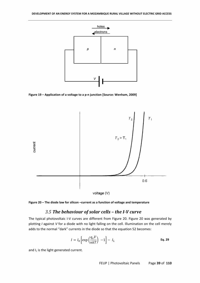
DEVELOPMENT OF AN ENERGY SYSTEM FOR A MOZAMBIQUE RURAL VILLAGE WITHOUT ELECTRIC GRID ACCESS
FEUP | Photovoltaic Panels Page 39 of 110
Figure 19 – Application of a voltage to a p-n junction [Source: Wenham, 2009]
Figure 20 – The diode law for silicon –current as a function of voltage and temperature
3.5 The behaviour of solar cells – the I-V curve
The typical photovoltaic I-V curves are different from Figure 20. Figure 20 was generated by
plotting I against V for a diode with no light falling on the cell. Illumination on the cell merely
adds to the normal “dark” currents in the diode so that the equation 52 becomes:
� 8 �� wexp o{�6%�s =1| = �� Eq. 29
and IL is the light generated current.
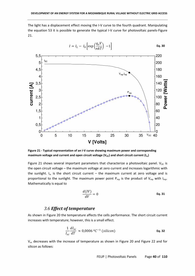
DEVELOPMENT OF AN ENERGY SYSTEM FOR A MOZAMBIQUE RURAL VILLAGE WITHOUT ELECTRIC GRID ACCESS
FEUP | Photovoltaic Panels Page 40 of 110
The light has a displacement effect moving the I-V curve to the fourth quadrant. Manipulating
the equation 53 it is possible to generate the typical I-V curve for photovoltaic panels-Figure
21.
� 8 �� = �� wexp o{�6%�s =1| Eq. 30
Figure 21 - Typical representation of an I-V curve showing maximum power and corresponding
maximum voltage and current and open circuit voltage (VOC) and short circuit current (Isc)
Figure 21 shows several important parameters that characterize a photovoltaic panel. VOC is
the open circuit voltage – the maximum voltage at zero current and increases logarithmic with
the sunlight. Isc is the short circuit current – the maximum current at zero voltage and is
proportional to the sunlight. The maximum power point Pmp is the product of Vmp with Imp.
Mathematically is equal to
.f��g.� 8 0 Eq. 31
3.6 Effect of temperature
As shown in Figure 20 the temperature affects the cells performance. The short circuit current
increases with temperature; however, this is a small effect.
1�J.�J.� C 0,0006 º�!" f�3234H6g Eq. 32
Voc decreases with the increase of temperature as shown in Figure 20 and Figure 22 and for
silicon as follows:
0 5 10 15 20 25 30 35 400
0,5
1
1,5
2
2,5
3
3,5
4
4,5
5
5,5
0
20
40
60
80
100
120
140
160
180
200
220
V [Volts]
cu
rre
nt
[A]
Po
we
r [W
att
s]
Pmp
Vmp,Imp
VOC
ISC
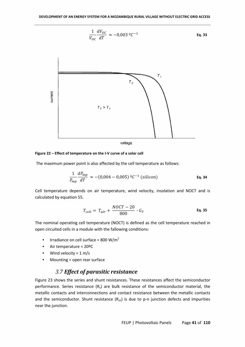
DEVELOPMENT OF AN ENERGY SYSTEM FOR A MOZAMBIQUE RURAL VILLAGE WITHOUT ELECTRIC GRID ACCESS
FEUP | Photovoltaic Panels Page 41 of 110
1���.���.� C =0,003 º�!" Eq. 33
Figure 22 – Effect of temperature on the I-V curve of a solar cell
The maximum power point is also affected by the cell temperature as follows:
1;�*.;�*.� C =f0,004 = 0,005g º�!" f�3234H6g Eq. 34
Cell temperature depends on air temperature, wind velocity, insolation and NOCT and is
calculated by equation 55.
� 8 ��i� h a��� = 20800 · �� Eq. 35
The nominal operating cell temperature (NOCT) is defined as the cell temperature reached in
open circuited cells in a module with the fallowing conditions:
• Irradiance on cell surface = 800 W/m2
• Air temperature = 20ºC
• Wind velocity = 1 m/s
• Mounting = open rear surface
3.7 Effect of parasitic resistance
Figure 23 shows the series and shunt resistances. These resistances affect the semiconductor
performance. Series resistance (Rs) are bulk resistance of the semiconductor material, the
metallic contacts and interconnections and contact resistance between the metallic contacts
and the semiconductor. Shunt resistance (Rsh) is due to p-n junction defects and impurities
near the junction.

DEVELOPMENT OF AN ENERGY SYSTEM FOR A MOZAMBIQUE RURAL VILLAGE WITHOUT ELECTRIC GRID ACCESS
FEUP | Photovoltaic Panels Page 42 of 110
Figure 23 – Parasitic shunt and serie resistances in a solar cell circuit
3.8 Photovoltaic modules in series and parallels
Photovoltaic modules connected in series and/or parallel permit to have different combination
(higher current or voltage). As shown in Figure 24 two photovoltaic modules connected in
various arrangements produce different currents or voltages. Series connections provide
higher voltages and parallel connections provide higher currents. Figure 26 and in Figure 27
shows the series connection that permits to have a higher voltage. If the two panels are
connected in parallel the voltage is the same but the current is the double.
Figure 24 – I-V curve for photovoltaic modules connected in various series and parallel arrangements

DEVELOPMENT OF AN ENERGY SYSTEM FOR A MOZAMBIQUE RURAL VILLAGE WITHOUT ELECTRIC GRID ACCESS
FEUP | EES equations and results Page 43 of 110
4. EES equations and results
The following pages will list the equations that were used to:
• Predict the radiation on a sloped photovoltaic panel
• Generate the photovoltaic I-V curve using manufactures catalogue data
• Pump controller and pump modulation
• Pumping system results
4.1 Solar radiation on a sloped photovoltaic array
To predict the radiation on a sloped photovoltaic array it is necessary to know the power that
comes from the sun. To characterize the radiation that comes from the sun there are two
important factors: 1) a geometric factor, because of the relative movement of earth around
the sun and the rotation of the earth around itself; 2) the solar extraterrestrial radiation that
reach the atmosphere, which varies over a year, but is modelled by a constant that is equal to
1367 W/m2. The extraterrestrial radiation incident on a horizontal surface is given by
�� 8 24 · 3600 · G��π o1 h 0,033 · cos 360 · 6365 s· �cosf�g · cosf�g · sin +J h �+J180 sin � sin ��
Eq. 36
And the hourly extraterrestrial radiation on a horizontal surface is equal to
�� 8 12 · 3600 · G��π o1 h 0,033 · cos 360 · 6365 s· ocosf�g · cosf�g · sinf+> = +"g h �f+> = +"g180 sin � sin �s
Eq. 37
The monthly average hourly radiation incident on a tilted surface is given by
�� 8 $� �� �:/� = ��� /�A L� h ��� /� o1 h cos f�g2 s h &� /� :f1 = cos f�g2 A � Eq. 38
To know �� it is necessary to calculate the monthly average clearness index $� 8 � ��� where
� is the global average monthly radiation given by meteorological data and is listed for each
month in Table 3. The meteorological data was taken by an average of 30 years measured in
Maniquenique station with latitude and longitude equal to 24º44’ and 33º32, respectively. GT
that appears after this chapter is in W/m2 and is calculated by multiplying ��, which is in
MJ/m2, by 277,778. To better understand this equations see appendix A.

DEVELOPMENT OF AN ENERGY SYSTEM FOR A MOZAMBIQUE RURAL VILLAGE WITHOUT ELECTRIC GRID ACCESS
FEUP | EES equations and results Page 44 of 110
Table 3 – Global average monthly radiation taken over a period of 30 years in the Maniquenique
station [Cuamba, 2006] and average day of the year [Duffie, 1991]
month � [kWh/m2/day] n month � [kWh/m
2/day] n
1 7,4 17 7 4,3 198
2 7 47 8 5 228
3 6,3 75 9 5,7 258
4 5,4 105 10 6,5 288
5 4,5 135 11 6,8 318
6 4,1 162 12 7,5 344
4.2 Photovoltaic I-V curve equations and results
This chapter summarise the equations that were used to model the photovoltaic array
behaviour. Table 4 list some general constants that are needed to plot the typical I-V curve.
The PV panels can be connected in various arrangements in series and/or in parallel. The total
generator area is equal do the area of a single photovoltaic panel times the number of panels
linked in series that formed a string and by multiplying the number of strings linked in parallel.
Figure 25 exemplifies one example to better understand. Taking this into account the
maximum power current and voltage will be affected by the respective number of panels
connect in parallel and series. The same is done to the open circuit voltage and the short
circuit current. The number of cells connected in series is also affected.
Table 4 - General constant values for photovoltaic I-V curve equations
Tair 25ºC
Tcel;ref 25ºC
GT;ref 1000 W/m2
Silicon bandgap (ε) 1,12 eV
rsh 1000 Ω

DEVELOPMENT OF AN ENERGY SYSTEM FOR A MOZAMBIQUE RURAL VILLAGE WITHOUT ELECTRIC GRID ACCESS
FEUP | EES equations and results Page 45 of 110
Figure 25 – Example of photovoltaic array with two parallel strings of three in series connection
[Source: Sunpumps catalogue]
To plot the photovoltaic I-V curve it is used the equation 48 and the other equations are used
to calculate necessary parameters in equation 48. The subscript ref means that the quantities
are measurements at reference conditions. The reference conditions are radiation of 1000
W/m2 and an ambient temperature of 25ºC. The result is plotted in Figure 26 and Figure 27. In
the modern cells the shunt resistance is very large and the last term of equation 48 can be
neglected [Duffie, 1991]. If the I-V curve in manufacture catalogue, at low voltage, exhibits a
pronounced negative slope instead of a nearly horizontal line as shown in Figure 24 then it is
necessary to consider the shunt resistance. Considering that the shunt resistance Rsh is infinite
there are 4 parameters to be determined in equation 48.
�E 8 �E ;Ji�� · 6/_� J�i · 6/_� *��� Eq. 39
�E 8 �E Ji�� · 6/_� J�i Eq. 40
�J 8 �J Ji�� · 6/_� *��� Eq. 41
��* 8 ��* Ji�� · 6/_� J�i Eq. 42
��* 8 ��* Ji�� · 6/_� *��� Eq. 43
The temperature coefficient of the open circuit voltage can be obtained from manufacturers
catalogue and is defined as

DEVELOPMENT OF AN ENERGY SYSTEM FOR A MOZAMBIQUE RURAL VILLAGE WITHOUT ELECTRIC GRID ACCESS
FEUP | EES equations and results Page 46 of 110
μ�;E 8 .���.� 8 ����;E · �E Eq. 44
Similarly the temperature coefficient of the short circuit current is equal to
μ�;J 8 .�J.� 8 ����;J · �J Eq. 45
6/ ;J 8 6/ ;Ji�� · 6/_� J�i Eq. 46
Another simplification is considering that the reference light current is equal to the short
circuit current [Duffie, 1991]:
��;�� 8 �J Eq. 47
� 8 �� = �� · wexp o� h � · /J 0�� s = 1| = w� h � · /J /Jt | Eq. 48
Solving equation 48 in order to I0 for Ie=0, IL=IL;ref and Ve=VOC the result is
��; �� 8 ��;�� · 5�G : =�E0��;��A Eq. 49
The light current is obtained by
�� 8 ����;�� · ���;�� h μ�;J · �� = � ;���� Eq. 50
And knowing I0;ref, Io is given by
����;�� 8 � � h 273,15� ;�� h 273,15�U · 5�G �� · 6/ ;J0��;�� · :1 = � � h 273,15� ;�� h 273,15�A� Eq. 51
The other variables are determined by the fallowing equations
0��;�� 8 μ�;E · �� ;�� h 273,15� = �E h � · 6/ ;Jμ�;J · �� ;�� h 273,15���;�� = 3
Eq. 52
0��0��;�� 8 � h 273,15� ;�� h 273,15 Eq. 53
/J 8 /J;�� 8 0��;�� · ln o1 = ��*��;�� s = ��* h �E��*
Eq. 54
� 8 ��i� h a��� = 20800 · �� Eq. 55

DEVELOPMENT OF AN ENERGY SYSTEM FOR A MOZAMBIQUE RURAL VILLAGE WITHOUT ELECTRIC GRID ACCESS
FEUP | EES equations and results Page 47 of 110
;�*E�� 8 � · � Eq. 56
;��� 8 ;�*E���E ;Ji�� · �� Eq. 57
)J J�� 8 #�;�E ;Ji�� · �� Eq. 58
Note that CCTV;oc is equal to "
�¡¢��¡¢�� and CCTI;sc is equal to
"�£¤
��£¤�� and they are temperature
coefficients.
Table 5 – ISOfotón ISO160 technical data
TNOCT 47ºC
nrcel;single 72
Acol;single 1,264 m2
Isc;single 4,87 A
Voc;single 44,2 V
Imp;single 4,5 A
Vmp;single 35,5 V
CCTI;sc 0,000254 1/ºC
CCTV;oc -0,00378 1/ºC
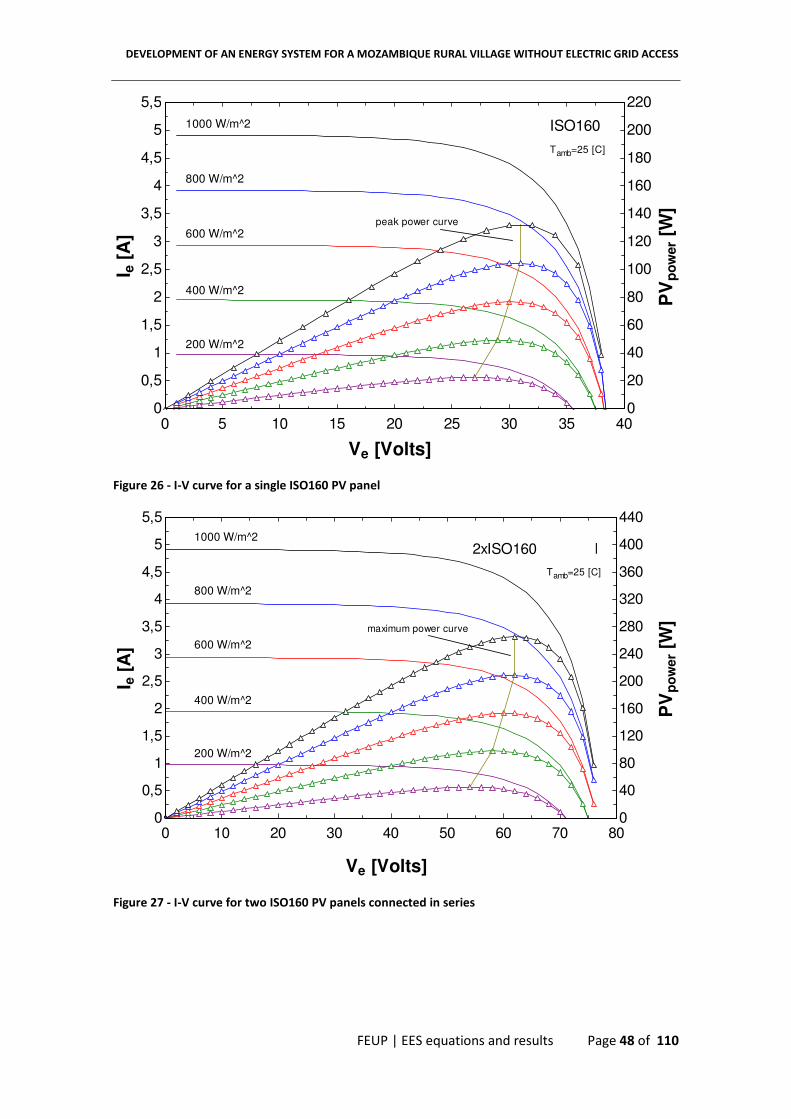
DEVELOPMENT OF AN ENERGY SYSTEM FOR A MOZAMBIQUE RURAL VILLAGE WITHOUT ELECTRIC GRID ACCESS
FEUP | EES equations and results Page 48 of 110
Figure 26 - I-V curve for a single ISO160 PV panel
Figure 27 - I-V curve for two ISO160 PV panels connected in series
0 5 10 15 20 25 30 35 400
0,5
1
1,5
2
2,5
3
3,5
4
4,5
5
5,5
0
20
40
60
80
100
120
140
160
180
200
220
Ve [Volts]
I e [
A]
Tamb=25 [C]
1000 W/m^2
800 W/m^2
600 W/m^2
400 W/m^2
200 W/m^2
PV
po
wer
[W]
peak power curve
ISO160
0 10 20 30 40 50 60 70 800
0,5
1
1,5
2
2,5
3
3,5
4
4,5
5
5,5
0
40
80
120
160
200
240
280
320
360
400
440
Tamb=25 [C]
1000 W/m^2
800 W/m^2
600 W/m^2
400 W/m^2
200 W/m^2
2xISO160 - Parallel
maximum power curve
Ve [Volts]
I e [
A]
PV
po
wer
[W]
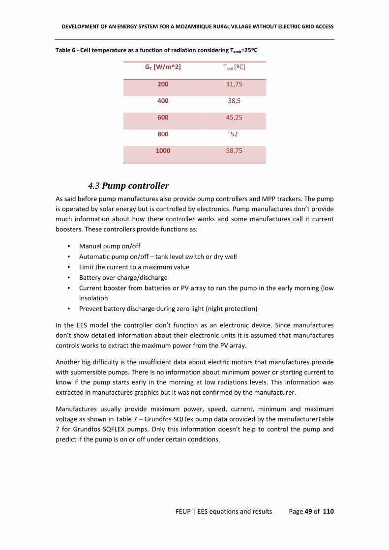
DEVELOPMENT OF AN ENERGY SYSTEM FOR A MOZAMBIQUE RURAL VILLAGE WITHOUT ELECTRIC GRID ACCESS
FEUP | EES equations and results Page 49 of 110
Table 6 - Cell temperature as a function of radiation considering Tamb=25ºC
GT [W/m^2] Tcell [ºC]
200 31,75
400 38,5
600 45,25
800 52
1000 58,75
4.3 Pump controller
As said before pump manufactures also provide pump controllers and MPP trackers. The pump
is operated by solar energy but is controlled by electronics. Pump manufactures don’t provide
much information about how there controller works and some manufactures call it current
boosters. These controllers provide functions as:
• Manual pump on/off
• Automatic pump on/off – tank level switch or dry well
• Limit the current to a maximum value
• Battery over charge/discharge
• Current booster from batteries or PV array to run the pump in the early morning (low
insolation
• Prevent battery discharge during zero light (night protection)
In the EES model the controller don’t function as an electronic device. Since manufactures
don’t show detailed information about their electronic units it is assumed that manufactures
controls works to extract the maximum power from the PV array.
Another big difficulty is the insufficient data about electric motors that manufactures provide
with submersible pumps. There is no information about minimum power or starting current to
know if the pump starts early in the morning at low radiations levels. This information was
extracted in manufactures graphics but it was not confirmed by the manufacturer.
Manufactures usually provide maximum power, speed, current, minimum and maximum
voltage as shown in Table 7 – Grundfos SQFlex pump data provided by the manufacturerTable
7 for Grundfos SQFLEX pumps. Only this information doesn’t help to control the pump and
predict if the pump is on or off under certain conditions.

DEVELOPMENT OF AN ENERGY SYSTEM FOR A MOZAMBIQUE RURAL VILLAGE WITHOUT ELECTRIC GRID ACCESS
FEUP | EES equations and results Page 50 of 110
Table 7 – Grundfos SQFlex pump data provided by the manufacturer
Motor Maximum Minimum
Voltage (VDC) 300 30
Current (A) 8,4 -
Power (W) 1400 -
Angular Speed (RPM) 3600 500
4.4 Maximum power point tracker
Since I-V curves are designed to dimension the photovoltaic system (series and/or parallel
connections) it is possible to know the Vmp for several solar radiations levels and use a
regression line to know the equation that relates Ve with GT. For ISO160 panel the equation is
in Figure 28. Using equation 73 for Ve=Vmp the maximum power current Imp is determined.
Figure 28 – Vmp as function of GT. Equation and quadratic error
4.5 Pump and water storage modulation – Grundfos SQFlex
Using Grundfos SQFlex catalogue (see Figure 17 for 5A-3 pump) it is possible to know the
volume flow as a function of input power and TDH.
Using Excel data analyser (regression) and using Table 10 and Table 11 data the regression constants results for 5A-3 pump and 2.5-2 (helical rotor pump)
are tabled in Table 8 and Table 9, respectively.
y = 2.478ln(x) + 13.99R² = 0.992
24
25
26
27
28
29
30
31
32
0 200 400 600 800 1000 1200
V_
mp
[v
olt
s]
G_T [W/m^2]
ISO160

DEVELOPMENT OF AN ENERGY SYSTEM FOR A MOZAMBIQUE RURAL VILLAGE WITHOUT ELECTRIC GRID ACCESS
FEUP | EES equations and results Page 51 of 110
Table 8 – Regression results for SQFlex 5A-3 pump
C0 C1 C2 C3 C4 C5 C6 C7 C8
-0,15 547,03 0,06 -25,47 0,00 0,00 0,00 2,91 769,15
Table 9 - Regression results for SQFlex 2.5-2 pump
C0 C1 C2 C3 C4 C5 C6 C7 C8
-0,01 741,31 -0,01 65,32 0,00 0,00 0,00 -5,72 5370,20
Table 10 – Grundfos SQFlex 5A-3 submersible pump data from Figure 17
H Q Motor Power
[m] [m^3/h] [W]
5,00 0,50 50,00
5,00 1,00 75,00
5,00 2,00 105,00
5,00 2,50 125,00
5,00 3,00 155,00
10,00 0,50 115,00
10,00 1,00 135,00
10,00 2,00 185,00
10,00 2,50 215,00
10,00 3,00 240,00
15,00 0,50 165,00
15,00 1,00 200,00
15,00 2,00 275,00
15,00 2,50 315,00
15,00 3,00 355,00
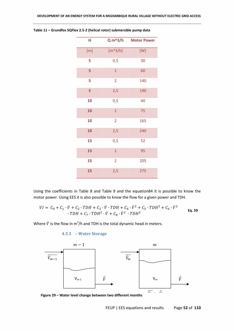
DEVELOPMENT OF AN ENERGY SYSTEM FOR A MOZAMBIQUE RURAL VILLAGE WITHOUT ELECTRIC GRID ACCESS
FEUP | EES equations and results Page 52 of 110
Table 11 – Grundfos SQFlex 2.5-2 (helical rotor) submersible pump data
H Q m^3/h Motor Power
[m] [m^3/h] [W]
5 0,5 30
5 1 60
5 2 140
5 2,5 190
10 0,5 40
10 1 75
10 2 165
10 2,5 240
15 0,5 52
15 1 95
15 2 205
15 2,5 275
Using the coefficients in Table 8 and Table 9 and the equation84 it is possible to know the
motor power. Using EES it is also possible to know the flow for a given power and TDH.
�� 8 �� h �" · �� h �> · �N� h �U · �� · �N� h �b · �� > h �Z · �N�> h �¥ · �� >· �N� h �¦ · �N�> · �� h �§ · �� > · �N�>
Eq. 59
Where �� is the flow in m3/h and TDH is the total dynamic head in meters.
4.5.1 – Water Storage
���!"�������
���
' = 1
Vm-1
�������
���
'
Vm
������� ¨ ���
� Figure 29 – Water level change between two different months

DEVELOPMENT OF AN ENERGY SYSTEM FOR A MOZAMBIQUE RURAL VILLAGE WITHOUT ELECTRIC GRID ACCESS
FEUP | EES equations and results Page 53 of 110
The volume balance in the storage system based in Figure 31 results in
�� 8 ��!" h �������� = ���� · 6�E��t Eq. 60
The subscript m means the month in question; nmonth is the number of days for the month m
and ��� is the mean consumption daily flow.
4.6 Water pumping system results
Two different pumps were analysed, and both of them are from the same manufacturer and
have the same cost. Table 12 summarizes the system configurations that were analysed.
Table 12 – Solar water system configuration that were analysed
System configuration
Number of PV 2; 3;4 or 5 ISO160 photovoltaic panels interconnected in series
Selected pump 1 Grundfos SQFlex HR 2.5-2 1 Grundfos SQFlex C 5A-3
Controller Grundfos C200 Grundfos C200
Table 13 and 14 shows the storage volume as a function of array tilted angle, initial storage
volume and using the 320 Wp system with the SQF helical rotor 2.5-2 pump and centrifugal 5A-
3 pump, respectively. For the first system the selected ��� was 16 m3/h and for the second
system (5A-3 pump) ��� = 15 m3/h. It was considered that the initial volume is equal to the total
storage volume.
Table 13 – Water volume in storage tank as a function of tilted array angle, initial storage volume and
month for 320Wp with SQF HR 2.5-2 pump system
Beta Initial
Volume months
[º] [m^3] Jun Jul Ago Set Out Nov Dez
0 45 0 0 0 0 45 45 45
10 45 0 0 0 0 45 45 45
20 45 1 0 0 1 41 45 45
30 45 26 15 8 5 23 45 45
40 45 39 40 32 13 0 0 20
50 45 41 41 21 0 0 0 0
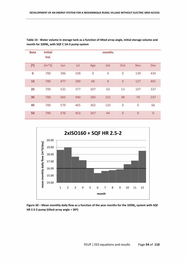
DEVELOPMENT OF AN ENERGY SYSTEM FOR A MOZAMBIQUE RURAL VILLAGE WITHOUT ELECTRIC GRID ACCESS
FEUP | EES equations and results Page 54 of 110
Table 14 - Water volume in storage tank as a function of tilted array angle, initial storage volume and
month for 320Wp with SQF C 5A-3 pump system
Beta Initial
Vol.
months
[º] [m^3] Jun Jul Ago Set Out Nov Dez
0 700 396 109 0 0 0 139 434
10 700 477 269 68 0 0 127 401
20 700 532 377 207 63 13 107 337
30 700 565 440 283 131 38 74 237
40 700 579 465 302 125 0 0 66
50 700 576 453 267 44 0 0 0
Figure 30 – Mean monthly daily flow as a function of the year months for the 320Wp system with SQF
HR 2.5-2 pump (tilted array angle = 30º)
14.00
15.00
16.00
17.00
18.00
19.00
20.00
1 2 3 4 5 6 7 8 9 10 11 12me
an
mo
nth
ly d
ail
y f
low
[m
^3
/da
y]
month
2xISO160 + SQF HR 2.5-2

DEVELOPMENT OF AN ENERGY SYSTEM FOR A MOZAMBIQUE RURAL VILLAGE WITHOUT ELECTRIC GRID ACCESS
FEUP | EES equations and results Page 55 of 110
Table 15 – Mean monthly daily flow [m3/day] for the system with SQF HR 2.5-2 pump and 320Wp
Jan Fev Mar Abr Mai Jun Jul Ago Set Out Nov Dez
18,6 19,0 17,7 17,2 16,1 15,4 15,7 15,8 15,9 16,6 17,1 18,5
Figure 31 - Mean monthly daily flow as a function of the year months for the 320Wp system with SQF
C 5A-3 pump (tilted array angle = 30º)
Table 16 - Mean monthly daily flow [m3/day] for the system with SQF C 5A-3 pump and 320Wp
Jan Fev Mar Abr Mai Jun Jul Ago Set Out Nov Dez
20,5 21,1 15,8 14,9 12,8 10,5 11,0 9,9 9,9 12,0 16,2 20,3
5.00
10.00
15.00
20.00
1 2 3 4 5 6 7 8 9 10 11 12
me
an
mo
nth
ly d
ail
y f
low
[m
^3
/h]
month
2xISO160 + SQF C 5A-3

DEVELOPMENT OF AN ENERGY SYSTEM FOR A MOZAMBIQUE RURAL VILLAGE WITHOUT ELECTRIC GRID ACCESS
FEUP | EES equations and results Page 56 of 110
Figure 32 - Annual predicted water volume as a function of array tilted angle and peak power using
SQF helical rotor (HR) 2.5-2 pump
Figure 33 - Annual predicted water volume as a function of array tilted angle and peak power using
SQF helical rotor (HR) 5A-3 pump
Table 17 - Annual predicted water volume as a function of array tilted angle using SQF helical rotor
(HR) 2.5-2 pump and a 320 Wp array
Beta [º] 0 10 20 30 40 50
Vanual [m3/year] 6092 6293 6284 6184 5942 5560
5000.0
6000.0
7000.0
8000.0
9000.0
10000.0
11000.0
0 10 20 30 40 50 60
an
nu
al
vo
lum
e [
m^
3/y
ea
r]
tilt angle [º]
SQF HR 2.5-2
320 Wp
480 Wp
640 Wp
800 Wp
4000
6000
8000
10000
12000
14000
16000
18000
0 10 20 30 40 50 60
wa
ter
vo
lum
e [
m^
3/y
ea
r]
tilt angle
SQF C 5A-3
320 Wp
480 Wp
640 Wp
800 Wp
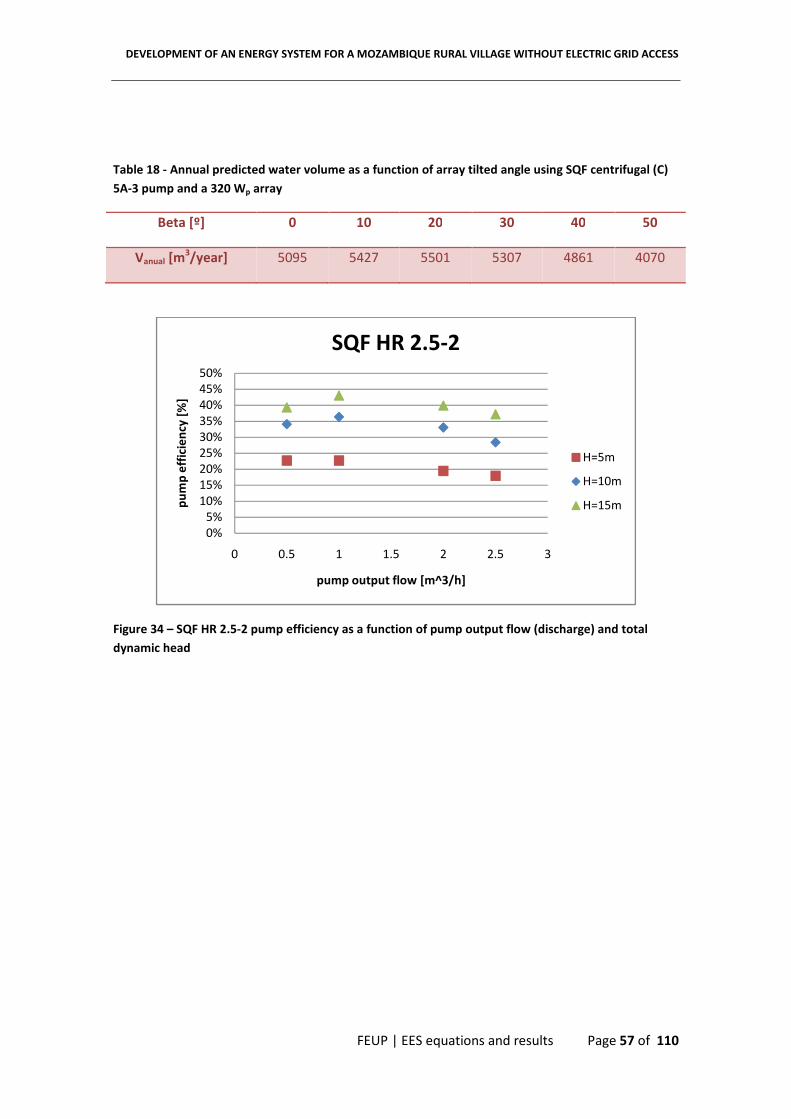
DEVELOPMENT OF AN ENERGY SYSTEM FOR A MOZAMBIQUE RURAL VILLAGE WITHOUT ELECTRIC GRID ACCESS
FEUP | EES equations and results Page 57 of 110
Table 18 - Annual predicted water volume as a function of array tilted angle using SQF centrifugal (C)
5A-3 pump and a 320 Wp array
Beta [º] 0 10 20 30 40 50
Vanual [m3/year] 5095 5427 5501 5307 4861 4070
Figure 34 – SQF HR 2.5-2 pump efficiency as a function of pump output flow (discharge) and total
dynamic head
0%5%
10%15%20%25%30%35%40%45%50%
0 0.5 1 1.5 2 2.5 3
pu
mp
eff
icie
ncy
[%
]
pump output flow [m^3/h]
SQF HR 2.5-2
H=5m
H=10m
H=15m
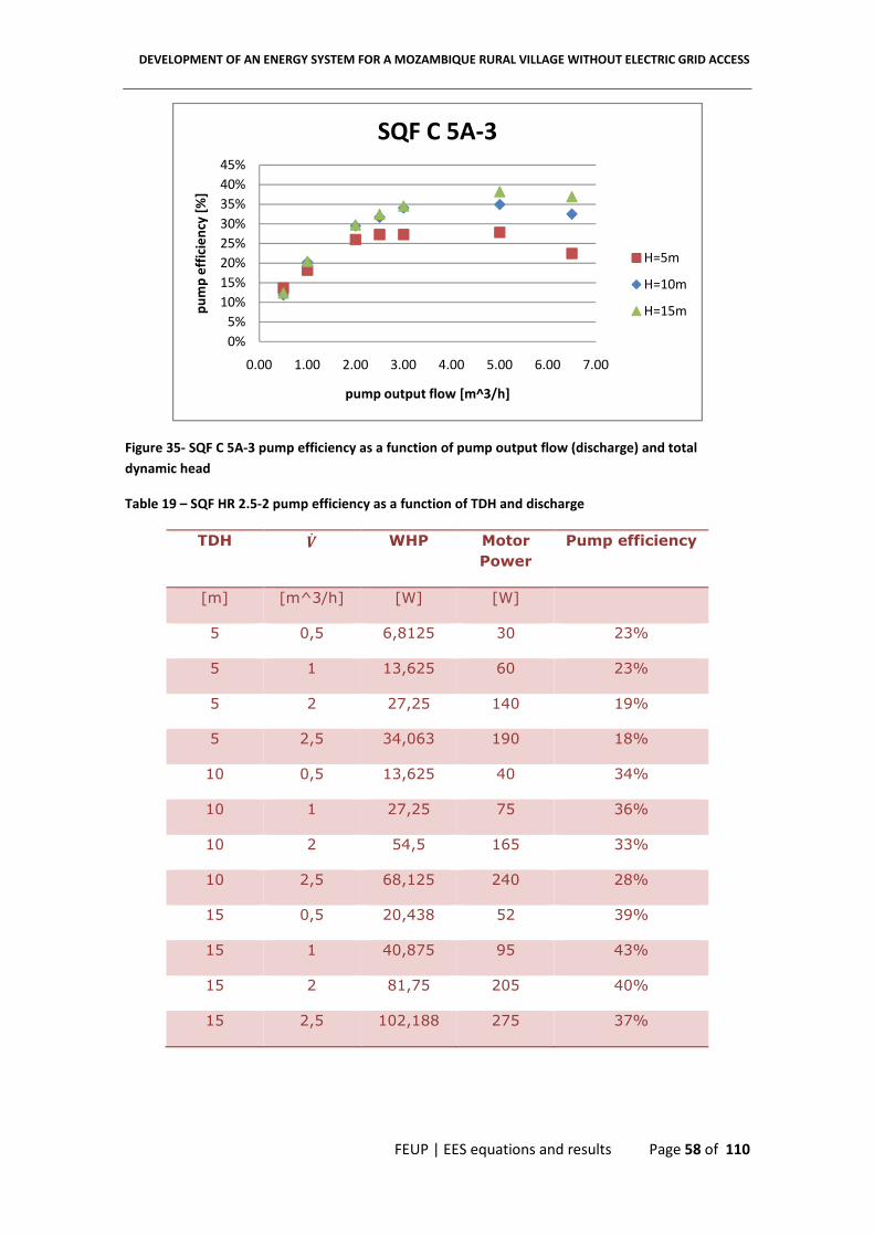
DEVELOPMENT OF AN ENERGY SYSTEM FOR A MOZAMBIQUE RURAL VILLAGE WITHOUT ELECTRIC GRID ACCESS
FEUP | EES equations and results Page 58 of 110
Figure 35- SQF C 5A-3 pump efficiency as a function of pump output flow (discharge) and total
dynamic head
Table 19 – SQF HR 2.5-2 pump efficiency as a function of TDH and discharge
TDH ©� WHP Motor
Power
Pump efficiency
[m] [m^3/h] [W] [W]
5 0,5 6,8125 30 23%
5 1 13,625 60 23%
5 2 27,25 140 19%
5 2,5 34,063 190 18%
10 0,5 13,625 40 34%
10 1 27,25 75 36%
10 2 54,5 165 33%
10 2,5 68,125 240 28%
15 0,5 20,438 52 39%
15 1 40,875 95 43%
15 2 81,75 205 40%
15 2,5 102,188 275 37%
0%
5%
10%
15%
20%
25%
30%
35%
40%
45%
0.00 1.00 2.00 3.00 4.00 5.00 6.00 7.00
pu
mp
eff
icie
ncy
[%
]
pump output flow [m^3/h]
SQF C 5A-3
H=5m
H=10m
H=15m
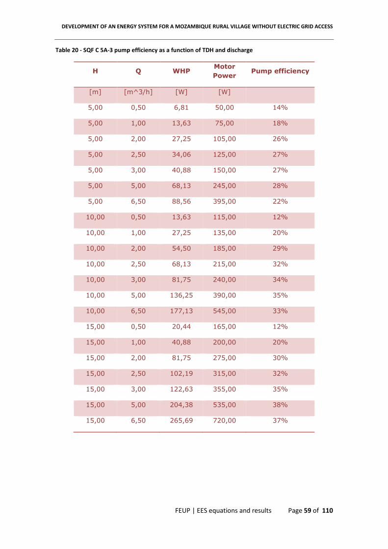
DEVELOPMENT OF AN ENERGY SYSTEM FOR A MOZAMBIQUE RURAL VILLAGE WITHOUT ELECTRIC GRID ACCESS
FEUP | EES equations and results Page 59 of 110
Table 20 - SQF C 5A-3 pump efficiency as a function of TDH and discharge
H Q WHP Motor
Power Pump efficiency
[m] [m^3/h] [W] [W]
5,00 0,50 6,81 50,00 14%
5,00 1,00 13,63 75,00 18%
5,00 2,00 27,25 105,00 26%
5,00 2,50 34,06 125,00 27%
5,00 3,00 40,88 150,00 27%
5,00 5,00 68,13 245,00 28%
5,00 6,50 88,56 395,00 22%
10,00 0,50 13,63 115,00 12%
10,00 1,00 27,25 135,00 20%
10,00 2,00 54,50 185,00 29%
10,00 2,50 68,13 215,00 32%
10,00 3,00 81,75 240,00 34%
10,00 5,00 136,25 390,00 35%
10,00 6,50 177,13 545,00 33%
15,00 0,50 20,44 165,00 12%
15,00 1,00 40,88 200,00 20%
15,00 2,00 81,75 275,00 30%
15,00 2,50 102,19 315,00 32%
15,00 3,00 122,63 355,00 35%
15,00 5,00 204,38 535,00 38%
15,00 6,50 265,69 720,00 37%

DEVELOPMENT OF AN ENERGY SYSTEM FOR A MOZAMBIQUE RURAL VILLAGE WITHOUT ELECTRIC GRID ACCESS
FEUP | EES equations and results Page 60 of 110
Figure 36 – System efficiency (ISO160 + SQF HR 2.5-2) as a function of radiation incident in the tilted
array and array peak power for H_sta=7m
Figure 37 - System efficiency (ISO160 + SQF C 5A-3) as a function of radiation incident in the tilted
array and array peak power for H_sta=7m
200 300 400 500 600 700 800 900 1000 11002,3
2,35
2,4
2,45
2,5
2,55
2,6
2,65
2,7
GT [W/m2]
2xISO160+SQFlex HR 2.5-22xISO160+SQFlex HR 2.5-2
3xISO160+SQFlex HR 2.5-23xISO160+SQFlex HR 2.5-2
4xISO160+SQFlex HR 2.5-24xISO160+SQFlex HR 2.5-2
5xISO160+SQFlex HR 2.5-25xISO160+SQFlex HR 2.5-2
Hest=7 [m]ηη ηη
syste
m
[%]
200 300 400 500 600 700 800 900 1000 11000
0,5
1
1,5
2
2,5
3
3,5
4
GT [W/m2]
Hest=7 [m]
2xISO160+SQFlex 5A-32xISO160+SQFlex 5A-3
3xISO160+SQFlex 5A-33xISO160+SQFlex 5A-3
4xISO160+SQFlex 5A-34xISO160+SQFlex 5A-3
5xISO160+SQFlex 5A-35xISO160+SQFlex 5A-3
ηη ηηsyste
m
[%]

DEVELOPMENT OF AN ENERGY SYSTEM FOR A MOZAMBIQUE RURAL VILLAGE WITHOUT ELECTRIC GRID ACCESS
FEUP | EES equations and results Page 61 of 110
Figure 38 - System efficiency (ISO160 + SQF HR 2.5-2) as a function of radiation incident in the tilted
array and array peak power for H_sta=11m
Figure 39 - System efficiency (ISO160 + SQF C 5A-3) as a function of radiation incident in the tilted
array and array peak power for H_sta=11m
200 300 400 500 600 700 800 900 1000 11002,6
2,8
3
3,2
3,4
3,6
3,8
GT [W/m2]
2xISO160+SQFlex HR 2.5-22xISO160+SQFlex HR 2.5-2
3xISO160+SQFlex HR 2.5-23xISO160+SQFlex HR 2.5-2
4xISO160+SQFlex HR 2.5-24xISO160+SQFlex HR 2.5-2
5xISO160+SQFlex HR 2.5-25xISO160+SQFlex HR 2.5-2
Hest=11 [m]ηη ηη s
yste
m
[%]
200 300 400 500 600 700 800 900 1000 11000
0,5
1
1,5
2
2,5
3
3,5
4
GT [W/m2]
ηη ηηsys
tem
[%
]
2xISO160+SQFlex 5A-32xISO160+SQFlex 5A-3
3xISO160+SQFlex 5A-33xISO160+SQFlex 5A-3
4xISO160+SQFlex 5A-34xISO160+SQFlex 5A-3
5xISO160+SQFlex 5A-35xISO160+SQFlex 5A-3
Hest=11 [m]

DEVELOPMENT OF AN ENERGY SYSTEM FOR A MOZAMBIQUE RURAL VILLAGE WITHOUT ELECTRIC GRID ACCESS
FEUP | EES equations and results Page 62 of 110
Figure 40 – Water discharged cost as a function of array peak power and pump type, based in a
system lifetime equal to 10 years
Figure 41 – Annual predicted discharged water volume as a function of array peak power and pump
type
0.025
0.030
0.035
0.040
0.045
0.050
0.055
200 300 400 500 600 700 800
wa
ter
cost
[€
/m^
3]
Array peak power [W]
Water cost
5A-3
2.5-2
4000
6000
8000
10000
12000
14000
16000
200 300 400 500 600 700 800 900
an
nu
al
vo
lum
e [
m^
3/y
ea
r]
Array peak power [W]
Annual volume
5A-3
2.5-2
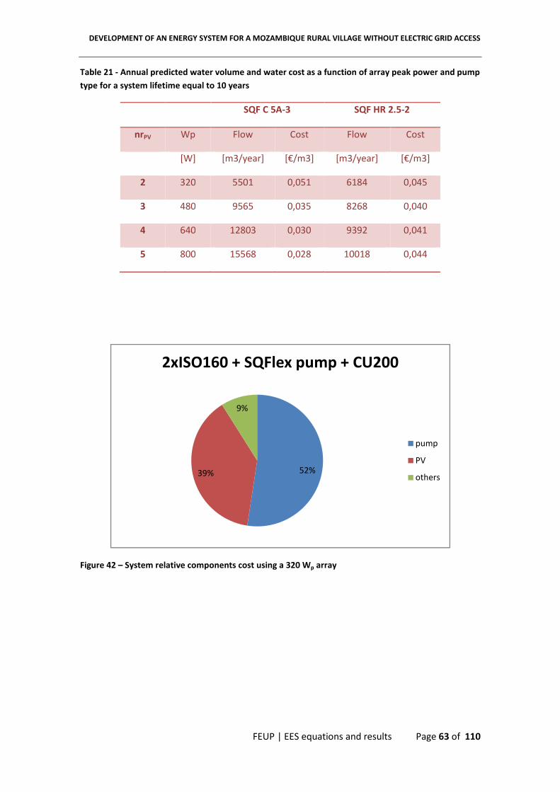
DEVELOPMENT OF AN ENERGY SYSTEM FOR A MOZAMBIQUE RURAL VILLAGE WITHOUT ELECTRIC GRID ACCESS
FEUP | EES equations and results Page 63 of 110
Table 21 - Annual predicted water volume and water cost as a function of array peak power and pump
type for a system lifetime equal to 10 years
SQF C 5A-3 SQF HR 2.5-2
nrPV Wp Flow Cost Flow Cost
[W] [m3/year] [€/m3] [m3/year] [€/m3]
2 320 5501 0,051 6184 0,045
3 480 9565 0,035 8268 0,040
4 640 12803 0,030 9392 0,041
5 800 15568 0,028 10018 0,044
Figure 42 – System relative components cost using a 320 Wp array
52%39%
9%
2xISO160 + SQFlex pump + CU200
pump
PV
others

DEVELOPMENT OF AN ENERGY SYSTEM FOR A MOZAMBIQUE RURAL VILLAGE WITHOUT ELECTRIC GRID ACCESS
FEUP | EES equations and results Page 64 of 110
Figure 43 - System relative components cost using a 800 Wp array
Table 22 – Total system cost, peak power cost and system relative components cost as a function of
array peak power (ISOfotón 160 peak power panels + Grundofos SQF pump + Grundfos CU200
controller)
Array
peak
power
Total
system
cost
System
cost pump PV others
[Wp] [€] [€/Wp]
160 2255 14,09 65,0% 23,9% 11,1%
320 2795 8,73 52,4% 38,6% 8,9%
480 3335 6,95 43,9% 48,6% 7,5%
640 3875 6,05 37,8% 55,7% 6,5%
800 4415 5,52 33,2% 61,2% 5,7%
33%
61%
6%
5xISO160 + SQFlex pump + CU200
pump
PV
others

DEVELOPMENT OF AN ENERGY SYSTEM FOR A MOZAMBIQUE RURAL VILLAGE WITHOUT ELECTRIC GRID ACCESS
FEUP | EES equations and results Page 65 of 110
Table 23 –System components unit price
Pump cost 1465 [€]1
CU 200 250 [€]1
PVcost 540 [€]
PVarea 1,264 [m2]
Cycle lifetime 10 [years]
Cycle life time is the period after witch costs of maintenance become higher than system costs. It was considered 10 years as a measure of precaution.
1 1€=1,297 USD

DEVELOPMENT OF AN ENERGY SYSTEM FOR A MOZAMBIQUE RURAL VILLAGE WITHOUT ELECTRIC GRID ACCESS
FEUP | Pumping system results discussion Page 66 of 110
5. Pumping system results discussion
Figure 30 shows the system match between the consumed flow and the mean predicted flow
that is clearly matched resulting in low volume reservoirs as shown in Table 13. As can be seen
in Table 14 and in Figure 31 the SQF 5A-3 pump is clearly unmatched with the consumption
resulting in too high water tank volumes.
Figure 32 and Figure 33 shows, respectively, the annual volume for the systems SQF HR 2.5-2
and SQF 5A-3 as a function of array tilt angle. For both systems the optimum tilt angle is 20º
but for minimum storage volume is 30º as shown in Table 13 and Table 14.
Figure 34 and Figure 35 shows that pump efficiency depends on the flow and the H produced
by the pump. For the helical rotor pump the BEP (43%) is for a head of 15m and a flow of 1
m3/h as seen in Table 19. The centrifugal pump BEP (38%) is for a head of 15m and a flow of 5
m3/h as showed in Table 20.
Figure 36 and Figure 37 (Hest=7m) shows that the system efficiency is higher for the SQF 5A-3
pump, especially for high radiation levels and higher photovoltaic array peak power. The
helical rotor pump system as a different behaviour for Hest=11m showing a better performance
for low radiation levels and low array peak power as illustrated in Figure 38. The centrifugal
pump also shows some differences for Hest=11m especially low performance in low radiation
levels and low peak powers. Figure 39 indicates that the pump only starts with a radiation level
higher than 400 W/m2 for the 320Wp array.
Based in a system lifetime of 10 years the water cost is lower increasing the array peak power
for the 5A-3 pump system as shown in Figure 40. With the same considerations the water cost
for the 2.5-2 pump is lower than the 5A-3 pump system for the array peak power of 320Wp.
The increase of array peak power in the centrifugal pump system decreases the water cost and
increases the mean annual volume as shown in Figure 41. Due to low performance of 2.5-2
pump at high flows the annual volume is lower compared to the 5A-3 pump for array peak
power of 480Wp. This is also the reason for the increase of water cost shown in Figure 40 for
the 2.5-2 pump.
Both pumps have the same initial cost and use the same pump controller as listed in Table 23.
Figure 42 and Figure 43 shows the relative components cost for different array peak power.
The objective of these charts is to show that using an expensive pump could justify and
increase in the number of photovoltaic panels. The total system cost are higher with the
increase of photovoltaic panels in the array but the system cost in €/Wp decreases as seen in
Table 22.
DEVELOPMENT OF AN ENERGY SYSTEM FOR A MOZAMBIQUE RURAL VILLAGE WITHOUT ELECTRIC GRID ACCESS
FEUP | Pumping system components selection Page 67 of 110
6. Pumping system components selection
6.1 Village Water needs
People in the village rationalises the water because they don’t have water in abundance near
them. They use dry latrine and wash the cloths in the river if possible. The system will try to
satisfy the water needs for 400 villagers. Considering that one person consumes about 40 liters
per day the system must produce about 16000 liters/day. To satisfy some needs of water to a
communitarian crop or cattle drinking it is possible to use the excess water production during
the summer.
6.2 Components selection
As said before the system must satisfy the village water needs with the lowest initial cost for
the association and at the same time with the lowest operating and maintenance costs.
Selecting a solar powered water system make the operation and maintenance costs very low in
comparison to diesel engines. The population is interested in the higher volume of water
possible per day and the association is interested in the lowest initial costs. Both are interested
in the highest reliable system.
It was assumed that the consumption is constant along the year and equal to 16 m3/day. It is
also possible that the volume of water needed by the population increases along the year and
through the years.
The system annual mean volume is equal to
������� 8 '506 .032- k2HI · 365 Eq. 61
If the mean daily flow is equal to 16 m3/h, the annual mean volume is equal to 5840 m3.
For the initial 16 m3/day the best pump is the SQF HR 2.5-2 with an array power of 320 Wp and
the reasons are:
• Up to 320 Wp this system has the lowest water cost
• Needs 45 m3 storage tanks to operate over a year without water shortage as predicted
by Table 13 considering a constant consumption daily volume
• As shown by Figure 30 the system always has 8 months with a mean daily flow equal
or higher than 16 m3/h
• Comparing Figure 30 and Figure 31 is easy to understand that the SQF C 5A-3 pump is
unmatched with the load and the result is a high storage volume as proved in Table 14
• For a tilted angle of 30º the system predicted annual volume is above the system
annual mean volume (5840 m3) as seen in Figure 32
This system is unsuited
• If the mean daily flow is too much higher than 16 m3/h
• If is predictable that the mean water volume consumption will rise above 27 m3/h
before the 10 years lifetime cycle

DEVELOPMENT OF AN ENERGY SYSTEM FOR A MOZAMBIQUE RURAL VILLAGE WITHOUT ELECTRIC GRID ACCESS
FEUP | Pumping system components selection Page 68 of 110
The SQF 5A-3 pump should be used if the daily flow is higher than 16 m^3/h, and with the
possibility to increase the number of photovoltaic modules the pump will operate even better
as shown in Figure 37 and Figure 39 and the water discharged cost will be lower compared to
the water cost for the SQF 2.5-2 pump as shown in Figure 40. SQF 5A-3 is a centrifugal pump
and the rated flow is 5 m3/h against the 2.5-2 pump that is a helical rotor pump with a rated
flow equal to 2,5 m3/h. The TDH over a year is low and helical rotor pumps are used in high
pumping heads with low flow, so if the daily flow is increased the installed pump should be
SQF 5A-3 with a higher array peak power. The system will me more flexible using the
centrifugal pump, because increasing the peak power in the array means that the system
water output will be much higher compared to the SQF 2.5-2 pump system. The proof is the
difference shown in Figure 41. In Figure 36 the system efficiency gets lower when the peak
power is increased. This is because the system efficiency is highly influenced by the pump
efficiency and the helical rotor pump efficiency is low at high flows.
The SQF 5A-3 pump system should be used with the possibility to adjust the consumption of
water over a year to avoid that the system is stopped for long periods in the summer. The
excess water produced during summer could be used to agriculture applications.

DEVELOPMENT OF AN ENERGY SYSTEM FOR A MOZAMBIQUE RURAL VILLAGE WITHOUT ELECTRIC GRID ACCESS
FEUP | Refrigeration system Page 69 of 110
7. Refrigeration system
7.1 Working fluids
The performance of real machines is determined by the properties of the working fluid. Some
working fluids were developed for determinate applications. Others were developed to work
in general conditions with some limitations. There is no working fluid that satisfies all the
requirements at the same time. For the vapour compression cycle the ideal properties for a
refrigerant are:
• High latent heat of vaporization
• High thermal conductivity
• High suction gas density
• Positive but not excessive pressures at evaporating and condensing conditions to avoid
air leakage in the system
• Critical temperature and triple point outside the working range
• Chemically stable, compatible with construction materials and miscible with lubricants
• Non-corrosive, non-toxic and non-flammable
• Environmentally friend
• Low cost production
The refrigerant is used to absorb heat at low temperature and low pressure and release heat
at a higher temperature and pressure. Most refrigerants undergo phase changes in the cycle.
This is why the refrigerant thermodynamic and physic properties are important.
7.1.1 Refrigerant designations
To uniform the nomenclature utilized for refrigerant fluids specific norms were developed, for
example the ASHRAE nomenclature. In a general way they are designated by the letter R
(refrigerant) plus a number that is related with chemical composition.
Refrigerants are classified in two great groups: synthetic and natural. Synthetic refrigerants are
produced with methane or ethane synthesizing with one or more hydrogen atoms replaced for
Chloride atoms, Fluor or Bromine. Syntactic refrigerants are divided into three groups:
CFC’s – As examples, R11, R12, R113, R114, R115, R500 and R502
HCFC’s – As examples, R22, R123, R141b and R142b
HFC’s – without chloride in there molecular structure – As examples, R32, R134a, R143a and
R152a
7.1.2 Absorption working fluids
Absorption cycles work with two fluids and there are two typical pairs: ammonia
(refrigerant)/water (absorber) and water (refrigerant)/lithium bromide (absorber). Other
working fluids exist but this two are widely used. Table 24 to Table 26 shows ammonia/water
and water/lithium bromide characteristics.

DEVELOPMENT OF AN ENERGY SYSTEM FOR A MOZAMBIQUE RURAL VILLAGE WITHOUT ELECTRIC GRID ACCESS
FEUP | Refrigeration system Page 70 of 110
Table 24 – Refrigerant properties [Source: Herold, 1996]
Property Ammonia/Water Water/Lithium bromide
High latent heat Good Excellent
Moderate vapour pressure Too high Too low
Low freezing temperature Excellent Limited application
Low viscosity Good Good
Table 25 – Absorbent properties [Source: Herold, 1996]
Property Ammonia/Water Water/Lithium bromide
Low vapour pressure Poor Excellent
Low viscosity Good Good
Table 26 – Mixture properties [Source: Herold, 1996]
Property Ammonia/Water Water/Lithium bromide
No solid phase Excellent Limited application
Low toxicity Poor Good
High affinity between
refrigerant and absorbent Good Good
7.2 Differences between compression and absorption
Ammonia/Water and Water/Lithium Bromide cycles
Absorption cycle that operates with ammonia/water have an additional equipment relative to
the absorption cycle that operates with water/lithium bromide. It is called rectifier. This is
because water is also volatile and when the solution is heated in the generator the formed
vapour is also a solution of ammonia and water. It is impossible to use a solution in the
condenser/evaporator because in this components heat is transferred at a constant
temperature. This situation is only possible in phase changes with pure substances. It is
necessary to rectify the vapour phase to increase the ammonia concentration (almost 100%)
before it is reached at the condenser. This system is more complex and has higher initial and
operating costs to the system. There are cases that only an ammonia/water system is used due
to water/lithium bromide limitations, i. e., lithium bromide crystallization or water freezing
(evaporator temperature less than 0ºC).
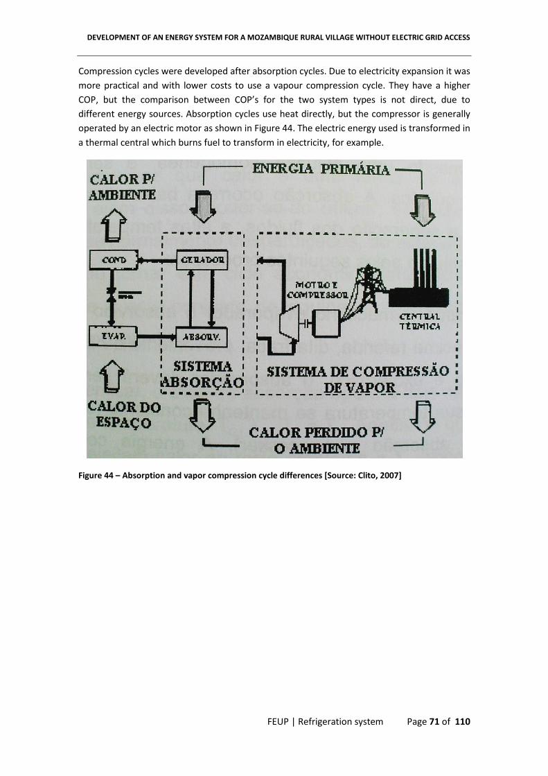
DEVELOPMENT OF AN ENERGY SYSTEM FOR A MOZAMBIQUE RURAL VILLAGE WITHOUT ELECTRIC GRID ACCESS
FEUP | Refrigeration system Page 71 of 110
Compression cycles were developed after absorption cycles. Due to electricity expansion it was
more practical and with lower costs to use a vapour compression cycle. They have a higher
COP, but the comparison between COP’s for the two system types is not direct, due to
different energy sources. Absorption cycles use heat directly, but the compressor is generally
operated by an electric motor as shown in Figure 44. The electric energy used is transformed in
a thermal central which burns fuel to transform in electricity, for example.
Figure 44 – Absorption and vapor compression cycle differences [Source: Clito, 2007]

DEVELOPMENT OF AN ENERGY SYSTEM FOR A MOZAMBIQUE RURAL VILLAGE WITHOUT ELECTRIC GRID ACCESS
FEUP | Thermodynamic properties of absorption working fluids Page 72 of 110
8. Thermodynamic properties of absorption working
fluids
Pure substances are thermodynamically characterized by two independent properties. In
mixtures it is necessary an additional property that quantifies its composition. This property is
called mass fraction and for binary mixture is equal to
� 8 '0�� Hk H65 4H'GH656FFHF02 '0�� Hk ªHF« 4H'GH656F� 8 '>'" h '> Eq. 62
The mass fraction of the other component is equal to (1-x). So component 1 is in its pure state
if x=0 and for the component 2 is for x=1.
8.1 Mixtures diagrams
When designing an absorption cycle the most important thermodynamic properties to be
considered are: pressure, temperature, mass fraction, enthalpy, entropy and specific volume.
8.1.1 Temperature-mass fraction diagram
Figure 45 shows a typical temperature-mass fraction diagram. To understand this diagram let´s
consider a subcooled mixture, point 1’, in equilibrium and heat is added to the system at
constant pressure. At certain point the point 2’ is reached and the first vapour bubble is
formed. The vapour is enriched in component B compared to the liquid. Its mass fraction is x2”.
This is the consequence of higher vapour pressure of component B compared to component A.
Point 3 is reached by additional heat where the mass fraction of the vapour (point 3”) is in
equilibrium with the remaining liquid. The mass fraction of the liquid is now indicated as 3’. At
this point, the amount of component B in the liquid phase has been reduced compared to
point 2’ while the vapour is enriched in component B. However, the vapour contains a lower
mass fraction of component B and more of component A. As the evaporation process
continues the point 4” is reached and the evaporation process is completed. The vapour at
point 4” has the same mass fraction as the initial subcooled liquid. The mass fraction of the
last liquid droplet is indicated by point 4’. Further heating produces superheated vapour at
point 5”.

DEVELOPMENT OF AN ENERGY SYSTEM FOR A MOZAMBIQUE RURAL VILLAGE WITHOUT ELECTRIC GRID ACCESS
FEUP | Thermodynamic properties of absorption working fluids Page 73 of 110
Figure 45 – Temperature mass fraction diagram – subcooled to superheated evolution
8.1.2 Pressure-temperature diagram
Usually this diagram is referred as the ln(P), -1/T diagram, Figure 46. The advantage of this
representation is the fact that the plots of saturation temperature versus saturation pressure
are almost straight lines for the most fluids mixtures when the mass fraction is constant.
Figure 46 – Water/LiBr vapour pressure temperature diagram
8.1.3 Enthalpy-mass fraction diagram
The enthalpy mass fraction diagram for water/lithium bromide is given by Figure 47. It found
wide applications for the design of absorption heat pumps. All lines on this diagram represent
saturation properties. The lower region represents the liquid phase, the middle region
represents the two-phase region and is bordered by the boiling and dew line and are isobar
lines. The enthalpy difference between the boiling and dew lines for x=0 and x=1 represents
the latent heat evaporation for each of the pure fluids. Within the two-phase region, the

DEVELOPMENT OF AN ENERGY SYSTEM FOR A MOZAMBIQUE RURAL VILLAGE WITHOUT ELECTRIC GRID ACCESS
FEUP | Thermodynamic properties of absorption working fluids Page 74 of 110
equilibrium between the vapour and liquid states can be connected by a tie line (isotherm and
isobar lines). For last the upper region is the superheated vapour area.
Figure 47 – Enthalpy mass fraction diagram for water/LiBr
Figure 48 - Enthalpy mass fraction diagram regions

DEVELOPMENT OF AN ENERGY SYSTEM FOR A MOZAMBIQUE RURAL VILLAGE WITHOUT ELECTRIC GRID ACCESS
FEUP | Thermodynamic processes with mixtures Page 75 of 110
9. Thermodynamic processes with mixtures
Considering the volume control in Figure 49 were (1-x) kg of substance 1 and x kg of substance
2, both at the same temperature, are introduced in the mixing chamber and the results is 1 kg
of mixture with a mass fraction x. If the mixture temperature is to remain constant (at
substance 1 and 2 temperature), for each kg of mixture it is necessary to give or extract heat
from the mixture chamber.
Sometimes the mixture heat is relative to the mass of substance 1 (q1) or 2 (q2) and not relative
to the mixture mass (q). Appling the first thermodynamic law to the volume control we have
{ 8 « = «" = «> Eq. 63
«" 8 f1 = �g«*�� " Eq. 64
«> 8 � «*�� > Eq. 65
hpure1 and hpure2 are the substances 1 and 2 enthalpy, respectively, in their pure state and
equation 63 can be written as
{ 8 « = �f1 = �g«*�� " h � «*�� >� Eq. 66
Knowing q, the mass fraction and the enthalpies of pure substances it is possible to calculate
from the anterior equation the mixture enthalpy. EES provides a library with procedures that
calculates several parameters for the water/lithium bromide mixture. In the literature the
water/lithium bromide enthalpy is given by
« 8 ¬ ��b
�v��� h � ¬ D�
b
�v��� h �> ¬ ��
b
�v��� Eq. 67
And the coefficients An,Bn,Cn and the equation domain are listed in Table 27.
Figure 49 – Two substance mixture with heat addition
'"� ; x1; T1; P1; h1
'>� ; x2; T2; P2; h2
'� ; x; T; P; h
{
f1 = �g%7
� %7
1 %7

DEVELOPMENT OF AN ENERGY SYSTEM FOR A MOZAMBIQUE RURAL VILLAGE WITHOUT ELECTRIC GRID ACCESS
FEUP | Thermodynamic processes with mixtures Page 76 of 110
Table 27 – Coefficients and equation 67 application domain [Source: Clito, 2007]
A0=-2024,33 B0=18,2829 C0=-3,7008214E-2
A1=163,309 B1=-1,1391757 C1=2,8877666E-3
A2=-4,88161 B2=3,248041E-2 C2=-8,1313015E-5
A3=6,302948E-2 B3=-4,034184E-4 C3=9,9116628E-7
A4=-2,913705E-4 B4=1,8520569E-6 C4=-4,4441207E-9
15<T<165 (ºC) 40<x<70% (LiBr)
9.1 Desorption
Desorption is the generation of vapour from the condensed phase (liquid or solid) of a mixture
of two or more components. The term implies that the vapour contains predominantly one
component in contrast to the evaporation process were all the components are assumed to
vaporize. Figure 50 exemplify the desorption process in a steady state and steady flow.
A vapor stream (2) is formed because heat is added to the initial liquid stream 1 and the
remaining liquid leaves the desorber from stream (3). The mass balance to the system results
in
'"� 8 '>� h 'U� Eq. 68
and for one component
'"� �" 8 '>� �> h 'U� �U Eq. 69
and dividing by the vapour mass flow '>� the solution circulating ratio, f, can be introduced
k 8 '"�'>� Eq. 70
Using the mass balance, equation 68,
k 8 �> = �U�" = �U Eq. 71
Figure 50 – Desorption process scheme
'"� ; x1; T1; P1; h1
(liquid)
(liquid)
(vapor)
��
'>� ; x2; T2; P2;h2
'U� ; x3; T3; P3; h2
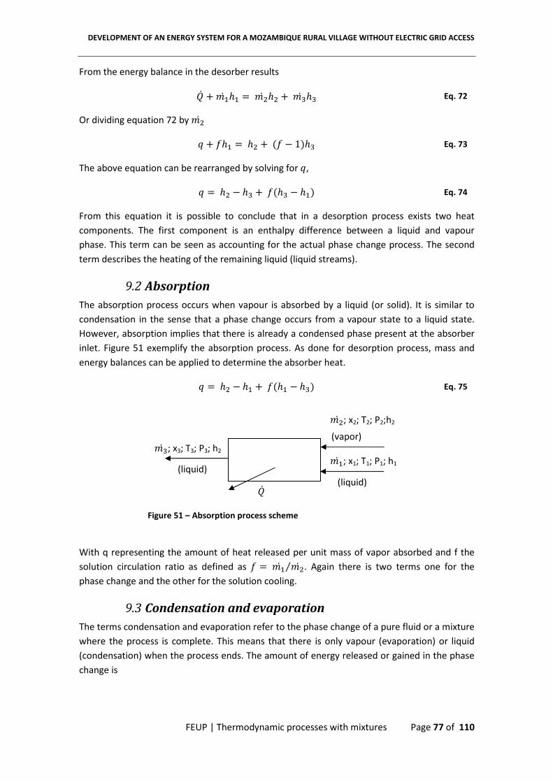
DEVELOPMENT OF AN ENERGY SYSTEM FOR A MOZAMBIQUE RURAL VILLAGE WITHOUT ELECTRIC GRID ACCESS
FEUP | Thermodynamic processes with mixtures Page 77 of 110
From the energy balance in the desorber results
�� h '"� «" 8 '>� «> h 'U� «U Eq. 72
Or dividing equation 72 by '>�
{ h k«" 8 «> h fk = 1g«U Eq. 73
The above equation can be rearranged by solving for {,
{ 8 «> = «U h kf«U = «"g Eq. 74
From this equation it is possible to conclude that in a desorption process exists two heat
components. The first component is an enthalpy difference between a liquid and vapour
phase. This term can be seen as accounting for the actual phase change process. The second
term describes the heating of the remaining liquid (liquid streams).
9.2 Absorption
The absorption process occurs when vapour is absorbed by a liquid (or solid). It is similar to
condensation in the sense that a phase change occurs from a vapour state to a liquid state.
However, absorption implies that there is already a condensed phase present at the absorber
inlet. Figure 51 exemplify the absorption process. As done for desorption process, mass and
energy balances can be applied to determine the absorber heat.
{ 8 «> = «" h kf«" = «Ug Eq. 75
With q representing the amount of heat released per unit mass of vapor absorbed and f the
solution circulation ratio as defined as k 8 '"� '>�⁄ . Again there is two terms one for the
phase change and the other for the solution cooling.
9.3 Condensation and evaporation
The terms condensation and evaporation refer to the phase change of a pure fluid or a mixture
where the process is complete. This means that there is only vapour (evaporation) or liquid
(condensation) when the process ends. The amount of energy released or gained in the phase
change is
'"� ; x1; T1; P1; h1 (liquid)
(liquid)
(vapor)
��
'>� ; x2; T2; P2;h2
'U� ; x3; T3; P3; h2
Figure 51 – Absorption process scheme

DEVELOPMENT OF AN ENERGY SYSTEM FOR A MOZAMBIQUE RURAL VILLAGE WITHOUT ELECTRIC GRID ACCESS
FEUP | Thermodynamic processes with mixtures Page 78 of 110
�®� 8 ¬ '®� f«E��;i = «i�;ig Eq. 76
and hout and hin are the enthalpies of the living and entering fluid streams.
9.4 Compression
The compression of vapour is often assumed to be isentropic to simplify the analysis and in
most instances the process occurs entirely in the vapour phase. Compressed vapour has a
higher pressure compared to the vapour pressure entering in the compressor. The
compression work is equal to
#� 8 ¬ '®� f«E��;i = «i�;ig Eq. 77
9.5 Pumping
In absorption systems liquid pumps are used to circulate the liquid streams through the piping
system and to convey the liquid from the low pressure side to the high pressure side of the
system. Assuming that the process is isentropic and the fluid is incompressible the pumping
work is equal to
#� 8 �Gti�t = G E�� ¯'�)* Eq. 78
phigh - plow represents the pressure difference across the pump, v is the specific volume of the
liquid, m the mass flow rate and )p the pump efficiency.
9.6 Throttling
In absorption cycles throttling devices are used to pass the liquid from the high pressure side
to the low pressure side by decreasing the liquid pressure. This process is assumed to be
adiabatic, resulting in a constant enthalpy process. The liquid temperature also varies. When a
liquid is throttled the outlet state can be a subcooled or a portion of the liquid can flash
(vaporize).
9.7 Water/Lithium bromide cycle
Figure 52 shows a single effect water/lithium bromide cycle. The energy source in the
generator (or desorber) could be any heat source, for example:
• Burning fossil fuels
• Using heat provided by renewable energies sources
• Heat rejected from electric centrals
• Other processes that rejects heat
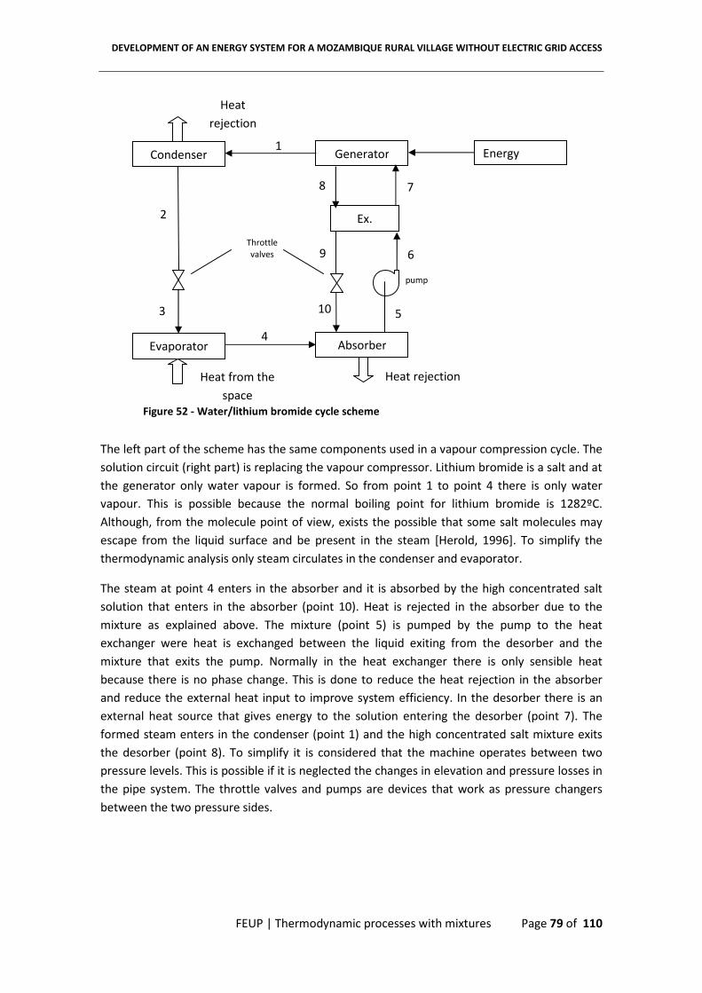
DEVELOPMENT OF AN ENERGY SYSTEM FOR A MOZAMBIQUE RURAL VILLAGE WITHOUT ELECTRIC GRID ACCESS
FEUP | Thermodynamic processes with mixtures Page 79 of 110
1
2
3
4
5
6
10
9
Generator Energy
Absorber
Heat rejection
pump
Heat
rejection
Condenser
Evaporator
Heat from the
space
Throttle valves
Ex.
7 8
The left part of the scheme has the same components used in a vapour compression cycle. The
solution circuit (right part) is replacing the vapour compressor. Lithium bromide is a salt and at
the generator only water vapour is formed. So from point 1 to point 4 there is only water
vapour. This is possible because the normal boiling point for lithium bromide is 1282ºC.
Although, from the molecule point of view, exists the possible that some salt molecules may
escape from the liquid surface and be present in the steam [Herold, 1996]. To simplify the
thermodynamic analysis only steam circulates in the condenser and evaporator.
The steam at point 4 enters in the absorber and it is absorbed by the high concentrated salt
solution that enters in the absorber (point 10). Heat is rejected in the absorber due to the
mixture as explained above. The mixture (point 5) is pumped by the pump to the heat
exchanger were heat is exchanged between the liquid exiting from the desorber and the
mixture that exits the pump. Normally in the heat exchanger there is only sensible heat
because there is no phase change. This is done to reduce the heat rejection in the absorber
and reduce the external heat input to improve system efficiency. In the desorber there is an
external heat source that gives energy to the solution entering the desorber (point 7). The
formed steam enters in the condenser (point 1) and the high concentrated salt mixture exits
the desorber (point 8). To simplify it is considered that the machine operates between two
pressure levels. This is possible if it is neglected the changes in elevation and pressure losses in
the pipe system. The throttle valves and pumps are devices that work as pressure changers
between the two pressure sides.
Figure 52 - Water/lithium bromide cycle scheme

DEVELOPMENT OF AN ENERGY SYSTEM FOR A MOZAMBIQUE RURAL VILLAGE WITHOUT ELECTRIC GRID ACCESS
FEUP | Thermodynamic processes with mixtures Page 80 of 110
9.8 Water/Lithium Bromide cycle limitations
The refrigerant is water so the temperature at the evaporator should be higher than 0ºC to
avoid refrigerant freezing. The refrigeration temperature for vaccines ranges from 2ºC to 8ºC
so using water as refrigerant is not a problem. If the temperature between the fluid circulating
in the evaporator and the refrigeration chamber is small then for the same heat transfer the
mass flow must be higher.
Another limitation is the lithium bromide mass fraction. When the mass fraction of LiBr
exceeds a limit the salt component precipitates. The solubility limit is a strong function of mass
fraction and temperature and weak function of pressure. In the cycle the mass fraction of LiBr
should not be higher than 70%. This could be avoided by lowering the sink temperature for
absorber cooling. Based on the properties of aqueous lithium bromide, low temperatures in
the absorber require lower absorption solution and thus avoiding the formation of
precipitates.
9.9 Vacuum requirements
Typical pressures in a LiBr absorption machine are subatmospheric. The pressure is
determined by the vapor pressure characteristics of the vapor fluid. In the condenser and
evaporator circulate essentially water and the pressure of these components is determined by
the operating temperature. These low pressures could result in system air leakage. LiBr in the
presence of oxygen is very aggressive to many metals. The presence of oxygen in the system
accelerates the corrosion process.
9.10 Pressure drops
As said before LiBr absorption machine operates under low pressures. Typical pressures are in
the order of 1 to 10 kPa. At this pressure the specific volume of saturated vapour is 129.2
kg/m^3 which results in high velocities. The pressure drop in the pipe system depends on the
fluid velocity and the higher the velocity the higher is the pressure drop. At these lower
pressures the slope of the vapour pressure curve of water is 14ºC/kPa indicating that small
pressure changes have a large influence on temperature.
9.11 Condenser and evaporator as heat exchangers
Thermodynamic cycles always perform between two sources, one with a high temperature
(hot source) and one with a lower temperature (cold source). During the entire cycle there are
heat exchanges between the refrigeration fluid and other medium fluids. Heat exchangers are
mechanical components that are responsible for heat transfer in the cycle. For the absorption
cycle there are 5 heat exchangers (condenser, evaporator, absorber, desorber and HX) as
shown in Figure 52 that works in different fluid phases.

DEVELOPMENT OF AN ENERGY SYSTEM FOR A MOZAMBIQUE RURAL VILLAGE WITHOUT ELECTRIC GRID ACCESS
FEUP | Thermodynamic processes with mixtures Page 81 of 110
Condensers are and indirect-contact heat exchanger in which the total heat rejected from the
refrigerant is removed by a cooling medium, usually air or water. Condensers are classified
based in the fluid that is used to promote the condenser cooling:
• Air-cooled condensers
• Water-cooled condensers
• Evaporative condensers
In air condensers the refrigerant condenses inside the tubes and air circulates in the outside of
the tubes. Because air as a low heat transfer coefficient the tubes are finned (higher heat
transfer area). There are two types of air condensers the ones that works with free convection
and the others work with forced convection. The first type is used in domestic application and
the air circulation is done by natural means (no machine). The second type uses a ventilator to
promote a higher heat transfer coefficient. Due to low specific heat capacity and high specific
volume of air implies a large volume to remove the condenser heat. The fans used to force the
volume of air makes noise and uses considerable amounts of power and this limits the
applications of forced air-cooled condensers.
Water condensers use cooled water to condensate the refrigerant. The higher heat capacity
and density of water makes it an ideal medium for condenser cooling requiring less volume of
water per second. The cooled water could be water from a lake, river or well near the plant or
from a cooling tower. Two types of water-cooled condensers are widely used for refrigeration
purposes: shell and tube and double tube condensers. A double tube condenser consists of
two tubes, one inside the other and water is pumped through the inner tube while refrigerant
flows in the space between the inner and outer tubes in a counterflow arrangement. Shell and
tube condensers are used when larger sizes of water-cooled condenser are necessary and this
arrangement is very compact for the same heat transfer capacity.
An evaporative condenser uses the evaporation of water spray to remove the latent heat of
condensation of the refrigerant during condensation. It is a simplified combination of a water-
cooled condenser and a cooling tower and is very efficient.
The last two types of condenser are generally used in industrial applications. For this project
the devices used for domestic applications are more suited, like the air-cooled condenser.
The purpose of the evaporator is to receive low-pressure, low temperature fluid from the
expansion valve and to bring it in close thermal contact with the load. The evaporator is also
an indirect contact heat exchanger and can be classified mainly into the following three types:
Dry expansion or direct-expansion (DX). The subcooled liquid that is throttled in the throttle
valve is sent to the evaporator and is totally vaporized and superheated to a certain degree in
the evaporator in its total length. These evaporators are a simple tube that is bended to the
desired form to fit in the refrigerator compartment and are commonly used in home
refrigerators.

DEVELOPMENT OF AN ENERGY SYSTEM FOR A MOZAMBIQUE RURAL VILLAGE WITHOUT ELECTRIC GRID ACCESS
FEUP | Thermodynamic processes with mixtures Page 82 of 110
Flooded refrigerant feed. In evaporators with flooded refrigerants feeds, liquid refrigerant is
fed through a throttling device and vaporizes outside the tubes within a shell. The refrigerant-
side surface area is always wetted by the liquid refrigerant, which results in a higher surface
heat-transfer coefficient.
Liquid overfeed. Liquid refrigerant is fed by a mechanical or gas pump and is then overfed to
each evaporator. The inner surface in overfeed evaporator is also wetted by liquid refrigerant.
9.12 Lithium bromide absorption system analysis
9.12.1 Mass flow balances
There are two important mass balances in the system. One is in the desorber as fallows
'¦� 8 '§� h '"� Eq. 79
The other is in the absorber
'Z� 8 '"�� h 'b� Eq. 80
The other mass balances are equal to 'Z� , '§� or '"� ,
'Z� 8 '¥� 8 '¦� Eq. 81
'§� 8 '°� 8 '"�� Eq. 82
'"� 8 '>� 8 'U� 8 'b� Eq. 83
The mass of lithium bromide that enters and exits from the desorber are the same, considering
that the water vapour (point 1) as zero salt content
'¦� �¦ 8 '§� �§ Eq. 84
Subtracting equation 84 to 79 results
'¦� f1 = �¦g 8 '§� f1 = �§g h '"� Eq. 85
Another important mass flow parameter is the solution circulation ratio, f,
k 8 '¦� '"� Eq. 86
Dividing equation 85 by '"� and solving the equation in order to f
k 8 '¦� '"� 8 �§�§ = �¦ Eq. 87

DEVELOPMENT OF AN ENERGY SYSTEM FOR A MOZAMBIQUE RURAL VILLAGE WITHOUT ELECTRIC GRID ACCESS
FEUP | Thermodynamic processes with mixtures Page 83 of 110
9.12.2 Energy balances
Using equation 76 and for i=1 (only one inlet and one exit) for the condenser and evaporator
the energy balance is
� � 8 '"� f«> = «"g Eq. 88
� � 8 '"� f«b = «Ug Eq. 89
The energy balance in the generator and the absorber results
�� � 8 '"� «" h '§� «§ = '¦� «¦ Eq. 90
�� � 8 'Z� «Z = 'b� «b = '"�� «"� Eq. 91
Applying equation 78 in the pump volume control the pump power consumption is equal to
#*��*� 8 fG¥ = GZg ¯ 'Z�)*��* Eq. 92
Considering that the heat exchanger is adiabatic (doesn’t exchange heat with the exterior), the
heat that the hot fluid lost is equal to the heat received by the cold fluid. This assumption
results in
�E �� 8 �tE�� 8 'Z� f«¦ = «¥g 8 '§� f«§ = «°g Eq. 93
The heat exchanger efficiency is equal to
� � 8 f«¦ = «¥gf«§ = «¥g Eq. 94
Assuming that throttling is considered adiabatically, resulting in a isenthalpic process
«U 8 «> Eq. 95
«"� 8 «° Eq. 96

DEVELOPMENT OF AN ENERGY SYSTEM FOR A MOZAMBIQUE RURAL VILLAGE WITHOUT ELECTRIC GRID ACCESS
FEUP | Thermodynamic processes with mixtures Page 84 of 110
9.13 Refrigeration capacity - Qe
The evaporator should extract an amount of energy in the refrigerator that balances the heat
losses by air leaks, heat transfers in the walls and the energy that is required to refrigerate a
determinate mass M from a higher temperature to a lower temperature. To simplify the
calculations air leaks are treated as a percentage of the evaporator capacity (50% higher),
based in the percentage calculated in [Clito,]. The refrigeration capacity Qe is calculated by
�� 8 ±²¬ ³�;ib
iv"´ · f��� = �i��g h µ4*f���� = �i��g
/5k/37. F3'5 ¶ · 1,5 Eq. 97
¬ ³�;ib
iv"8 ¬ 1L�E�� i
b
iv" Eq. 98
Based in Figures 54 and 55 Rtotal i and Rtotal 4 are equal to
L�E�� i 8 Lj,�� i · L���,�� iLj,�� i h L���,�� i h ¬ LE�� ·U
·v"h Lj,i�� i · L���,i�� iLj,i�� i h L���,i�� i Eq. 99
L�E�� b 8 Lj,�� i · L���,�� iLj,�� i h L���,�� i h ¬ LE�� ·U
·v" Eq. 100
1
2
3
4
L
W
H
Figure 53 – Refrigerator physical measures and surfaces

DEVELOPMENT OF AN ENERGY SYSTEM FOR A MOZAMBIQUE RURAL VILLAGE WITHOUT ELECTRIC GRID ACCESS
FEUP | Thermodynamic processes with mixtures Page 85 of 110
The index “i” is used for different surfaces as illustrated in Figure 59 and the index j is linked to
the different wall layers. Equation 99 is different from equation 100 because the radiation in
the bottom is neglected due to possible surface bottom contact.
Figure 54 – Heat transfer resistance scheme for general refrigerator walls
Figure 55 - Heat transfer resistance scheme - bottom refrigerator wall
9.13.1 Heat transfer by conduction through the walls
�E�� � 8 ¸ · � ∆�5 Eq. 101
�E�� � 8 ∆�LE�� Eq. 102
LE��;i 8 5i¸i � Eq. 103
Rcond is the thermal resistance of the layer against heat conduction. The walls are composed by
three layers so there is three Rcond. The material properties are listed in Table 28.
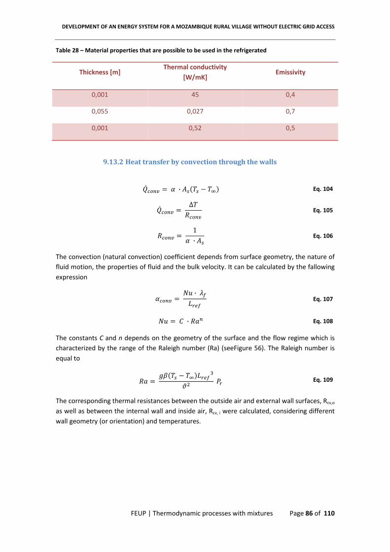
DEVELOPMENT OF AN ENERGY SYSTEM FOR A MOZAMBIQUE RURAL VILLAGE WITHOUT ELECTRIC GRID ACCESS
FEUP | Thermodynamic processes with mixtures Page 86 of 110
Table 28 – Material properties that are possible to be used in the refrigerated
Thickness [m] Thermal conductivity
[W/mK] Emissivity
0,001 45 0,4
0,055 0,027 0,7
0,001 0,52 0,5
9.13.2 Heat transfer by convection through the walls
��E�j 8 ¹ · �Jf�J = �ºg Eq. 104
��E�j 8 ∆�LE�j Eq. 105
LE�j 8 1¹ · �J Eq. 106
The convection (natural convection) coefficient depends from surface geometry, the nature of
fluid motion, the properties of fluid and the bulk velocity. It can be calculated by the fallowing
expression
¹E�j 8 a1 · ¸�l�� Eq. 107
a1 8 � · L0� Eq. 108
The constants C and n depends on the geometry of the surface and the flow regime which is
characterized by the range of the Raleigh number (Ra) (seeFigure 56). The Raleigh number is
equal to
L0 8 7�f�J = �ºgl��U»> ;� Eq. 109
The corresponding thermal resistances between the outside air and external wall surfaces, Rcv,o
as well as between the internal wall and inside air, Rcv, i were calculated, considering different
wall geometry (or orientation) and temperatures.
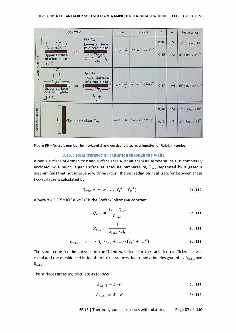
DEVELOPMENT OF AN ENERGY SYSTEM FOR A MOZAMBIQUE RURAL VILLAGE WITHOUT ELECTRIC GRID ACCESS
FEUP | Thermodynamic processes with mixtures Page 87 of 110
Figure 56 – Nusselt number for horizontal and vertical plates as a function of Raleigh number
9.13.3 Heat transfer by radiation through the walls
When a surface of emissivity ε and surface area As at an absolute temperature Tp is completely
enclosed by a much larger surface at absolute temperature, Tsup, separated by a gaseous
medium (air) that not intervene with radiation, the net radiation heat transfer between these
two surfaces is calculated by
����� 8 � · ¼ · �J��Jb = �ºb� Eq. 110
Where σ = 5,729x10-8 W/m2K4 is the Stefan-Boltzmann constant.
����� 8 �* = �J�*L��� Eq. 111
L��� 8 1¹��� · �J Eq. 112
¹��� 8 � · ¼ · �J · f�J h �ºg · ��J> h �º>� Eq. 113
The same done for the convection coefficient was done for the radiation coefficient. It was
calculated the outside and inside thermal resistances due to radiation designated by Rrad, o and
Rrad, i.
The surfaces areas are calculate as follows
���;" 8 l · � Eq. 114
���;> 8 # · � Eq. 115

DEVELOPMENT OF AN ENERGY SYSTEM FOR A MOZAMBIQUE RURAL VILLAGE WITHOUT ELECTRIC GRID ACCESS
FEUP | Thermodynamic processes with mixtures Page 88 of 110
���;U 8 l · # Eq. 116
�i��;" 8 fl = 2 · I022�ti�JJg · f� = 2 · I022�ti�JJg Eq. 117
�i��;> 8 f#=2 · I022�ti�JJg · f�=2 · I022�ti�JJg Eq. 118
�i�;U 8 fl = 2 · I022�ti�JJg · f# = 2 · I022�ti�JJg Eq. 119
9.14 Cycle thermodynamic states
Assuming that only steam circulates in points 1, 2, 3 and 4 the respective enthalpies are
calculate by knowing the pressure, temperature and/or vapour quality (at least two
properties). As considered before there is two pressure levels. Points 1, 2, 6, 7, 8, 9 are at the
higher pressure and points 3, 4, 5 and 10 are at the lower pressure. From here several
assumptions could result in very different results with different system COP. For example,
point 4 could be superheated water vapour or saturated water vapour (vapour quality = 1).
The difference between the lower and higher pressure sides could be large or very small
depending on the system operating temperatures. The mass flow circulating in the pump could
vary between several values resulting in different, higher or lower, mass flow rate at point 1.
The heat exchanger efficiency affects the system efficiency and operation points.
Table 29 – Base system operating points
Point State Notes
1 Superheated water vapour Assuming zero salt content
2 Saturated liquid Vapour quality = 0
3 Vapour liquid water state Due to water flash during throttling
4 Saturated water vapour Vapour quality = 1
5 Saturated liquid solution Vapour quality = 0
6 Subcooled liquid solution Higher pressure, constant temperature
7 Subcooled liquid solution State calculated from heat exchanger model
8 Saturated liquid solution Vapor quality = 0
9 Subcooled liquid solution State calculated from heat exchanger mode
10 Vapour liquid solution state Due to water flash during throttling

DEVELOPMENT OF AN ENERGY SYSTEM FOR A MOZAMBIQUE RURAL VILLAGE WITHOUT ELECTRIC GRID ACCESS
FEUP | Absorption System EES results Page 89 of 110
10. Absorption System EES results
Table 30 – Refrigerator surfaces global heat transfer coefficient and respective resistances
Surface
number Rcond,i Rcv_e,i Rcv_i,i Rrad_e,i Rrad_i,i Rtotal Ur;i
[K/W] [K/W] [K/W] [K/W] [K/W] [K/W] [W/K]
1 1,359 0,334 0,574 0,277 0,334 1,722 0,581
2 2,039 0,500 0,898 0,416 0,522 2,596 0,385
3 1,359 0,233 1,017 0,277 0,334 1,737 0,576
4 1,359 0,655 0,448
2,462 0,406
Table 31 – Refrigerator exterior dimensions
L [m] W [m] H [m]
1,5 1 1
Table 32 – Exterior and interior surfaces areas
Surface
number Aext Aint
[m2] [m2]
1 1,5 1,228
2 1 0,785
3 1,5 1,228
4 1,5 1,228

DEVELOPMENT OF AN ENERGY SYSTEM FOR A MOZAMBIQUE RURAL VILLAGE WITHOUT ELECTRIC GRID ACCESS
FEUP | Absorption System EES results Page 90 of 110
Table 33 – Absorption system constants
ΔTrefrig 120 s
Tenter 8 ºC
Tsurface 25 ºC
T[1] 80 ºC
Patm 103 kPa
Text 35 ºC
½¾� 180 W
PCIButane 45E6 J/kg
effpump 0,45
effHX 0,6
Lfin 0,11 m
finS 0,015 m
Lc 1 m
effger 0,7
efffin 0,36
UAe 50 W/K
xhigh 0,62
xlow 0,47

DEVELOPMENT OF AN ENERGY SYSTEM FOR A MOZAMBIQUE RURAL VILLAGE WITHOUT ELECTRIC GRID ACCESS
FEUP | Absorption System EES results Page 91 of 110
Figure 57 – Effect of solution heat exchanger on COP
Table 34 – Effect of solution heat exchanger on COP and refrigerator mean air temperature
HXeff COP Tair;i
[C]
0 0,699 6,378
0,1 0,708 6,313
0,2 0,718 6,245
0,3 0,729 6,174
0,4 0,740 6,101
0,5 0,751 6,024
0,6 0,763 5,943
0,7 0,775 5,859
0,8 0,788 5,77
0,9 0,801 5,676
1 0,815 5,577
0 0,2 0,4 0,6 0,8 10,68
0,7
0,72
0,74
0,76
0,78
0,8
0,82
effp
CO
P
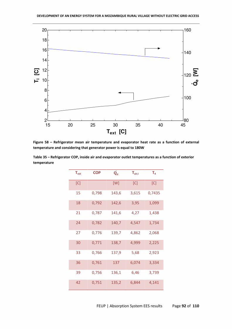
DEVELOPMENT OF AN ENERGY SYSTEM FOR A MOZAMBIQUE RURAL VILLAGE WITHOUT ELECTRIC GRID ACCESS
FEUP | Absorption System EES results Page 92 of 110
Figure 58 – Refrigerator mean air temperature and evaporator heat rate as a function of external
temperature and considering that generator power is equal to 180W
Table 35 – Refrigerator COP, inside air and evaporator outlet temperatures as a function of exterior
temperature
Text COP ½¿� Tair;i T4
[C]
[W] [C] [C]
15 0,798 143,6 3,615 0,7435
18 0,792 142,6 3,95 1,099
21 0,787 141,6 4,27 1,438
24 0,782 140,7 4,547 1,734
27 0,776 139,7 4,862 2,068
30 0,771 138,7 4,999 2,225
33 0,766 137,9 5,68 2,923
36 0,761 137 6,074 3,334
39 0,756 136,1 6,46 3,739
42 0,751 135,2 6,844 4,141
15 20 25 30 35 40 452
4
6
8
10
12
14
16
18
20
80
100
120
140
160
Text [C]
Ti [
C]
Qe
[W]
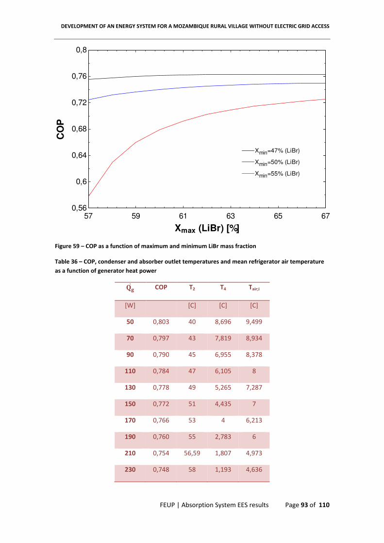
DEVELOPMENT OF AN ENERGY SYSTEM FOR A MOZAMBIQUE RURAL VILLAGE WITHOUT ELECTRIC GRID ACCESS
FEUP | Absorption System EES results Page 93 of 110
Figure 59 – COP as a function of maximum and minimum LiBr mass fraction
Table 36 – COP, condenser and absorber outlet temperatures and mean refrigerator air temperature
as a function of generator heat power
½¾� COP T2 T4 Tair;i
[W] [C] [C] [C]
50 0,803 40 8,696 9,499
70 0,797 43 7,819 8,934
90 0,790 45 6,955 8,378
110 0,784 47 6,105 8
130 0,778 49 5,265 7,287
150 0,772 51 4,435 7
170 0,766 53 4 6,213
190 0,760 55 2,783 6
210 0,754 56,59 1,807 4,973
230 0,748 58 1,193 4,636
57 59 61 63 65 670,56
0,6
0,64
0,68
0,72
0,76
0,8
Xmax (LiBr) [%]
CO
P
Xmin=47% (LiBr)Xmin=47% (LiBr)
Xmin=50% (LiBr)Xmin=50% (LiBr)
Xmin=55% (LiBr)Xmin=55% (LiBr)

DEVELOPMENT OF AN ENERGY SYSTEM FOR A MOZAMBIQUE RURAL VILLAGE WITHOUT ELECTRIC GRID ACCESS
FEUP | Absorption System EES results Page 94 of 110
Figure 60 – COP and refrigerator mean air temperature as a function of generator heat rate
Table 37 – Condenser length effect on condenser outlet temperature, COP, evaporator heat rate,
refrigerator inside mean air temperature and evaporator outlet temperature
Lc T2 COP ½¿� Tair;i T4
[m] [C]
[W] [C] [C]
0,5 70,68 0,7273 131 6,185 3,566
0,6 65,22 0,7392 133 6,104 3,442
0,7 61,2 0,7476 135 6,047 3,355
0,8 58,11 0,7538 136 6,005 3,291
0,9 55,67 0,7587 137 5,971 3,239
1 53,7 0,7627 137 5,943 3,198
1,1 52,07 0,766 138 5,921 3,163
1,2 50,71 0,7688 138 5,902 3,134
1,3 49,54 0,7712 139 5,885 3,109
50 80 110 140 170 200 2300,74
0,76
0,78
0,8
0,82
0,84
0,86
0,88
0,9
2
3
4
5
6
7
8
9
10
Qg [W]
CO
P
Ti [
C]

DEVELOPMENT OF AN ENERGY SYSTEM FOR A MOZAMBIQUE RURAL VILLAGE WITHOUT ELECTRIC GRID ACCESS
FEUP | Absorption System EES results Page 95 of 110
Figure 61 – COP and evaporator heat rate as a function of condenser length
Figure 62 – COP and heat transfer rate for generator, evaporator, and solution heat exchanger as a
function of pump flow
0,4 0,6 0,8 1 1,2 1,4 1,60,72
0,74
0,76
0,78
0,8
120
125
130
135
140
Lc [m]
CO
P
[%]
Qe
[W]
0,5 0,6 0,7 0,8 0,9 10,5
0,55
0,6
0,65
0,7
0,75
0,8
0
40
80
120
160
200
240
280
pumpflow [kg/h]
CO
P
[%]
He
at
tra
ns
fer
rate
r [W
]
GeneratorGenerator
EvaporatorEvaporator
Solution heat exchangerSolution heat exchanger
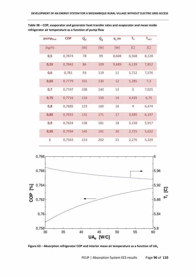
DEVELOPMENT OF AN ENERGY SYSTEM FOR A MOZAMBIQUE RURAL VILLAGE WITHOUT ELECTRIC GRID ACCESS
FEUP | Absorption System EES results Page 96 of 110
Table 38 – COP, evaporator and generator heat transfer rates and evaporator and mean inside
refrigerator air temperature as a function of pump flow
pumpflow COP ½¿� ½¾� q_ex T4 Tair;i
[kg/h] [W] [W] [W] [C] [C]
0,5 0,7874 78 99 8,608 6,568 8,128
0,55 0,7842 86 109 9,689 6,139 7,852
0,6 0,781 93 119 11 5,712 7,576
0,65 0,7779 101 130 12 5,285 7,3
0,7 0,7747 108 140 13 5 7,025
0,75 0,7716 116 150 14 4,435 6,75
0,8 0,7685 123 160 16 4 6,474
0,85 0,7655 131 171 17 3,585 6,197
0,9 0,7624 138 181 18 3,158 5,917
0,95 0,7594 145 191 20 2,725 5,632
1 0,7563 153 202 21 2,276 5,329
Figure 63 – Absorption refrigerator COP and interior mean air temperature as a function of UAe
30 35 40 45 50 55 600,758
0,76
0,762
0,764
0,766
0,768
5,8
5,84
5,88
5,92
5,96
6
UAe [W/C]
CO
P
[%]
Ti [
C]

DEVELOPMENT OF AN ENERGY SYSTEM FOR A MOZAMBIQUE RURAL VILLAGE WITHOUT ELECTRIC GRID ACCESS
FEUP | Page 97 of 110
Table 39 - Absorption refrigerator COP, evaporator heat rate, interior mean air temperature and
outlet evaporator temperature as a function of UAe
UAe COP ½¿� Tair;i T4
[W/C] [W] [C] [C]
30 0,7589 137 6 1,416
33 0,7597 137 5,964 2
36 0,7605 137 5,959 2,156
39 0,7611 137 5,955 2,442
42 0,7616 137 5,951 2,687
45 0,762 137 5,948 3
48 0,7624 137 5,945 3,086
51 0,7628 137 5,943 3
54 0,7631 137,4 5,941 3,397
57 0,7634 137 5,939 3,528
60 0,7636 138 5,937 3,646

DEVELOPMENT OF AN ENERGY SYSTEM FOR A MOZAMBIQUE RURAL VILLAGE WITHOUT ELECTRIC GRID ACCESS
FEUP | Absorption system results discussion Page 98 of 110
11. Absorption system results discussion
The coefficient of performance of absorption system is highly influenced by the solution heat
exchanger efficiency as seen in Figure 57 – Effect of solution heat exchanger on COPFigure 57.
The difference is almost 10% less performance when compared to 80% heat exchanger
efficiency and by not having a solution heat exchanger.
Figure 58 shows the refrigerator mean air temperature as a function of exterior air
temperature considering that the generator power is 180W. The heat gained by the
refrigerator decreases with the increase of exterior air temperature because the inside
temperature increases. The machine input power is constant and the evaporator operating
temperature also increases and this influence the evaporator heat rate that decreases with the
increase of outside air temperature as shown in Table 35. It is important that the machine has
a generator gas flow valve to control the heat input in the generator.
The mass fraction of LiBr circulating between the generator and absorber influences the cycle
performance as shown in Figure 59. The max COP occurs when the difference between xmax
and xmin is maximum. The weak solution in LiBr is influenced by the pressure and temperature
of absorber and the strong solution that exits the generator is dependent of the pressure and
temperature of generator. To avoid LiBr crystallization problems there should be a difference
between the xmax of cycle and the 70% maximum LiBr concentration by controlling the
absorber and desorber temperature.
The power in the generator influences the machine performance. As shown in Figure 60 the
higher the generator power is the lowest is the performance of the machine, but the effect in
the inside air temperature of refrigerator is higher. Considering the selected configuration for
the condenser (Lc=1m) it is clearly unmatched for the generator power (180W) as can be seen
in Table 36 where the outlet condenser temperature is higher than 53ºC at outside air
temperature of 35ºC. Figure 61 shows the COP is higher with a higher condenser length and an
increase in the evaporator heat rate for a generator power of 180W. As can be seen in Table
37 the effect on inside air temperature is less than 0,4ºC compared to have a 0,5m or 1,5m
condenser length.
With the outlet water vapour temperature equal to 80ºC, the higher the solution flow
circulated by the pump is, the higher is the generator, evaporator and solution heat exchanger
heat rates as shown in Figure 62. As commented before the COP is lower because the
generator power is higher, but the effect on refrigerator inside temperature is higher as shown
again in Table 38.
The global heat transfer coefficient for the evaporator has little effect on COP and on the
inside air temperature as shown in Figure 63. However the effect on the outlet evaporator
temperature is not negligible because for the same heat transfer the difference between
outlet evaporator temperature and refrigerator inside air temperature is higher.

DEVELOPMENT OF AN ENERGY SYSTEM FOR A MOZAMBIQUE RURAL VILLAGE WITHOUT ELECTRIC GRID ACCESS
FEUP | Selecting Vaccine refrigerator Page 99 of 110
12. Selecting Vaccine refrigerator
World Health Organization (WHO) created a guideline for manufacturers of vaccine
refrigerators. A certain product of a manufacture is actually qualified if specific Performance,
Quality and Safety (PQS) requirements are satisfied. The anterior performance specifications
and verification protocols were the PIS that were replaced by the PQS in 2007. For
refrigerators or combined refrigerator-icepack freeze with an absorption cycle the PQS
performance requirements are:
• The acceptable temperature range for storing vaccine is +2°C to +8°C
• Holdover time: The time in hours during which all points in the vaccine compartment
remain between +2°C and +10°C, at the maximum ambient temperature of the
temperature zone for which the appliance is rated, after the fuel supply has been
disconnected (minimum of 3 hours)
• Hot zone appliances must operate at a steady +43°C ambient temperature and over
a+43°C/+25°C day/night cycling temperature range
• Moderate zone: Moderate zone appliances must operate at a steady +27°C ambient
temperature and over a+27°C/+10°C day/night cycling temperature range
• Temperate zone: Temperate zone appliances must operate at a steady +32°C ambient
temperature and over a+32°C/+15°C day/night cycling temperature range
• Fuel supply is natural gas, propane or kerosene
• Externally readable cabinet-mounted gas or vapour pressure dial thermometer
• The product is to be designed to achieve a maintenance-free life of not less than 10
years apart from re-fueling, wick replacement and trimming (kerosene units) flue
cleaning, routine de-frosting and cleaning and replacement of batteries (if any)

DEVELOPMENT OF AN ENERGY SYSTEM FOR A MOZAMBIQUE RURAL VILLAGE WITHOUT ELECTRIC GRID ACCESS
FEUP | Selecting Vaccine refrigerator Page 100 of 110
12.1 Product datasheet
Table 40 – Zero Appliances GR265 G/E product performance information
Ice pack Freezer, With Vaccine +32°C 4.2kg/24hrs
+43°C 1.8kg/24hrs
Hold Over Time During Power Cut
5.5 hours(+32°C)
1.5 hours (+43°C)
Power Consumption: Gas
660g/24hrs (+32ºC)
(without a gas thermostat)
770g/24hrs (+43ºC)
(without a gas thermostat)
Table 41 – Sibir V110GE product performance information according to EPI/PROC/5
Safe Ice pack freezing 32 ambient (ºC) 1,2kg
Hold over time 32 ambient (ºC) 4,02h
EPI specification E3/RF.2
Table 42 - Sibir V110GE product input/consumption information
Gas inlet pressure (Propane) 30 mbar
Max input 170 W
Gas consumption 385 g/24h

DEVELOPMENT OF AN ENERGY SYSTEM FOR A MOZAMBIQUE RURAL VILLAGE WITHOUT ELECTRIC GRID ACCESS
FEUP | Selecting Vaccine refrigerator Page 101 of 110
Table 43 - Zero Appliances GR265 G/E product specifications
Vaccine Storage Capacity Refrigerator 57L
Frozen Ice Pack Storage Capacity Freezer 9.6L
Manufacturers Gross Volume Refrigerator 180L
Freezer 32L
External Dimensions (HxWxL) (Not Boxed)
150x60x68cm
Type Of Kerosene Burner/Gas Jet Size
Jet Size 13
Table 44 - Sibir V110GE product specifications
Net capacity 102 l
Net vaccine storage capacity 20 l
Net freezer capacity 15 l
DEVELOPMENT OF AN ENERGY SYSTEM FOR A MOZAMBIQUE RURAL VILLAGE WITHOUT ELECTRIC GRID ACCESS
FEUP | Conclusions Page 102 of 110
13. Conclusions
The match between the consumed and the outputted water volume by the pump can be
evaluated by the total storage volume. The lowest volume is always the best and it is not
recommended for this specific case a zero storage volume. Two or three days are the
minimum recommended storage volume. Considering a 16 m3/day the minimum storage
volume should range between 32 to 48 m3.
The optimum angle over a year could be the angle that optimises the water pump output or
benefit the months with the lowest water pump output. A fixed angle of 30º benefit the
months with the lowest water pump output.
To satisfy the villagers water needs the best studied pump is the SQF centrifugal 5A-3 pump
with an array peak power higher than 320Wp. The SQF helical rotor is limited to 10000 m3/year
and is recommended to be installed in places with higher static heads. Possibly the initial
system cost will be between 3000€ to 5000€ because it was not considered the storage tanks
and support structure costs, labour hand and transportation. The price depends also from
photovoltaic support structure and the number of installed panels.
The coefficient of performance of absorption system is highly influenced by the solution heat
exchanger efficiency. It’s also influenced by the environment air temperature and solution
concentration between the absorber and the generator. The condenser length has also an
impact in the COP and the global heat transfer in the evaporator also influences the COP but as
a higher impact in the evaporator outside temperature.
It’s not possible to select the best refrigerator because it depends from the dimension of the
future health center. The selected refrigerators in the above chapter are very different from
the point of view of vaccine capacity, holdover time, propane consumption and safe ice pack
freezing capacity at outside air temperature of 32ºC. Both of them are approved by the PIS but
they are not yet approved by the new PQS performance specifications. Only a few models are
prequalified to be approved by the new PQS performance specifications. For high vaccine
capacity the best one is the Zero Appliances GR265 G/E, but for low vaccine capacity the best
one is the Sibir V110GE refrigerator. In the new prequalified list there are only products that
work with a compression cycle, using AC or DC electric motors and some models uses
photovoltaic panels with batteries. This could mean that the vaccine refrigerators
manufactures are excluding the use of LP gas or kerosene as a heat source, because it’s not
easy to find a PIS certificated product that works with an absorption cycle.

DEVELOPMENT OF AN ENERGY SYSTEM FOR A MOZAMBIQUE RURAL VILLAGE WITHOUT ELECTRIC GRID ACCESS
FEUP | References Page 103 of 110
14. References
[1] Afonso, C. Félix, “Sebenta de refrigeração”, Aefeup Editorial, 2007
[2] Afonso, C., Castro, M., Matos, J. – “Air infiltration on domestic refrigerators: the influence
of the magnetic seals”
[3] ASHRAE, “Refrigeration: 1998 ASHRAE handbook”, 2nd edition, Am. Soc. Heat., Refrig., [4]
Air-Cond. Eng., USA, 1998
[5] Buschermohle, M. J., Burns, R. T., “Solar-Powered Livestock Watering Systems”
[6] Çengel, Yunus A., Boles, Michael A. - “Thermodynamics: an engineering approach” - 5th
edition in SI units. - Boston: McGraw-Hill/Higher Education, cop. 2006
[7] Cuamba, B. C., et. al.- “A solar energy resources assessment in Mozambique”- Journal of
Energy in Southern Africa, Vol. 17 Number 4, 2006
[8] Dinçer, I., “Refrigeration Systems and Application”, Wiley, West Sussex, 2003
[9] Dougherty, Robert L., “Centrifugal pumps” - September 2007, Das Press
[10] Duffie, John A., Beckman, William A., “Solar engineering of thermal processes” - 2nd ed. -
New York [etc.]: John Wiley & Sons, cop. 1991
[11] Fiaschi, D., Graniglia, R., Giampaolo M., 2005 – “Improving the effectiveness of solar
pumping systems by using modular centrifugal pumps with variable rotational speed”, Solar
Energy, Vol. 79 – pag. 234-244
[12] Gottlieb, I. - “Practical electrical motor handbook” – Elsevier Science, 1997
[13] Herold, K. E.; Radermacher, Reinhard; Klein, Sanford A., “Absorption chillers and heat
pumps”, CRC Press, 1996
[14] Herold, Keith E., Radermacher Reinhard, Klein, Sanford A., “Absorption chillers and heat
pumps”, CRC Press, cop. 1996
[16] Huacuz, J. M., Flores, R., Agredano, J., 1995 – “Field Performance of Lead-Acid Batteries in
Photovoltaic Rural Electrification Kits”, Solar Energy, Vol.55 – pag. 287-295
[17] Incropera, Frank P., “Fundamentals of heat and mass transfer” - 6th ed. - Danvers: John
Wiley & Sons, cop. 2007
[18] Messenger, Roger A., Ventre, Jerry - “Photovoltaic systems engineering” - 2nd ed. - CRC
Press, cop. 2004
[19] Odeh I., Yohanis Y.G., Norton B., “Economic viability of photovoltaic water pumping
systems”, July 2005 [Solar Energy 80 (2006) 850–860]
[20] Odeh, I., 2006 “Influence of pumping head, insolation and PV array size on PV water
pumping system performance”, Solar Energy, Vol. 80 – pag. 51-64

DEVELOPMENT OF AN ENERGY SYSTEM FOR A MOZAMBIQUE RURAL VILLAGE WITHOUT ELECTRIC GRID ACCESS
FEUP | References Page 104 of 110
[21] SELF, “A cost and reliability comparison between solar and diesel powered pumps”, Jully
2008
[22] Short, T.D., P. Thompson, 2003 – “Breaking the mould: solar water pumping – the
challenges and the reality”, Solar Energy ,Vol. 75 – pag. 1-9
[23] Stoecker, W.F., Jones., J. W. “Refrigeration and air conditioning” - 2nd ed. -
Auckland: McGraw- Hill Book Company, 1982
[24] Vick, B. D., Clark, R. N., 1996 – “Performance of Wind-Electric and Solar-PV Water
Pumping Systems for Watering Livestock”, Jornal of Solar Energy Engineering, Vol. 118 - pag.
212-216
[25] Wang, Shan K. – “Handbook of Air Conditioning and Refrigeration”, McGraw-Hill, 2nd
editon, 2000
[26] Wenham, Stuart R., “Applied Photovoltaics” - 2nd. - London : Earthscan, 2009
[27] White, Frank M. (2003), “Fluid Mechanics” - 6th ed. - McGraw-Hill/Higher
Education : Boston [etc.], cop. 2008
Websites
[28] E03 Refrigerators and freezers for storing vaccines and freezing icepacks -
http://www.who.int/immunization_standards/vaccine_quality/pqs_e03_fridges_freezers/en/i
ndex.html
[29] Electrical Impedance - http://en.wikipedia.org/wiki/Electrical_impedance
[30] Grundfos WEBCAPS/SQFlex catalogue–
http://net.grundfos.com/Appl/WebCAPS/InitCtrl?mode=13
[31] Millennium Development Goals - http://unstats.un.org/unsd/mdg/Default.aspx
[32] Naps System - http://www.napssystems.com/
[33] Performance, Quality and Safety (PQS) - Prequalified equipment -
http://www.who.int/immunization_standards/vaccine_quality/e03_prequalified_equip/en/ind
ex.html
[34] Solar Energy for Africa - http://www.solarafrica.org/
[35] Sunpumps products catalogue - http://www.sunpumps.com/ProductsClient.aspx
[36] Vaccine refrigerator - http://en.wikipedia.org/wiki/Vaccine_refrigerator
[37] WHO -
http://www.who.int/immunization_standards/vaccine_quality/pqs_e03_rf02_1.pdf
[38] Wikipedia Millennium Development Goals -
http://en.wikipedia.org/wiki/Millennium_Development_Goals
DEVELOPMENT OF AN ENERGY SYSTEM FOR A MOZAMBIQUE RURAL VILLAGE WITHOUT ELECTRIC GRID ACCESS
FEUP | Appendix A - Solar radiation Page 105 of 110
Appendix A - Solar radiation
Before analysing the photovoltaic panels it is important to understand the energy source – the
sun. Studying solar geometry helps to know the sun position, the direction of beam radiation
incident on surfaces of various orientations and shading. To better understand the solar
geometry it is necessary to define important definitions.
A.1 - Definitions
Air mass m is the ratio of the mass of atmosphere through which beam radiation passes to the
mass it would pass through if the sun were at the zenith (shortest path). For zenith angle
between 0º and 70º at sea level m is equal to:
' 8 1/ cosfÀÁg Eq. A.1
Beam radiation is the direct solar radiation. In other words is the solar radiation that wasn’t
scattered by the atmosphere.
Diffuse radiation is the solar radiation received from the sun after its direction has been
changed by scattering the atmosphere.
Total solar radiation is the sum of beam and diffuse radiation on a surface.
Irradiance (G) is the rate at which radiant energy is incident on a surface, per unit area of
surface.
Irradiation is the incident energy per unit area on a surface found by integrating irradiance
over a specified time. The subscript H is used for insolation for a day. The symbol I is used for
insolation for an hour. The symbols H and I can represent beam, diffuse, or total and can be on
surfaces of any orientation. Subscripts on G, H and I are as follows: 0 refers to extraterrestrial
radiation, b and d refer to beam and diffuse radiation; T and n refers to radiation on a tilted
plane and normal plane; If the plane is horizontal the symbols doesn’t have any subscript.
A.1.1 - Direction of beam radiation
The following definitions refer to angles that describe the geometric relationships between a
plane and earth at any time. The angles are as follows:
Latitude (φ) site angular location relative to the equator between -90º and 90º (north-positive
or south - negative).
Declination (δ), the angular position of the sun at solar noon with respect to the plane of the
equator, north positive; -23,45º< δ<23,45º
� 8 23,45 · sin o360 · 284 h 6365 s Eq. A.2
Slope (β), the angle between the plane of the surface and the horizontal plane; 0º<β<90º.
Surface azimuth angle (γ), the deviation of the projection on a horizontal plane of the normal
to the surface from the local meridian, with zero due south, east negative and west positive;
-180º< δsurface <180º

DEVELOPMENT OF AN ENERGY SYSTEM FOR A MOZAMBIQUE RURAL VILLAGE WITHOUT ELECTRIC GRID ACCESS
FEUP | Appendix A - Solar radiation Page 106 of 110
Hour angle (+), the angular displacement of the sun east or west of the local meridian due to
the rotation of the earth on its axis at 15º per hour, morning negative and afternoon positive.
Angle of incidence (θ) the angle between the beam radiation on a surface and the normal to
that surface
Zenith angle (θz) the angle between the vertical and the line to the sun
Solar altitude angle (αs), the angle between the horizontal and the line to the sun
(complement to the zenith angle)
Solar azimuth angle (γs), the angular displacement from south of the projection of the beam
radiation on the horizontal plane
Figure A.1 – Zenith angle (θz), slope (β), surface azimuth angle, and solar azimuth angle (ϒs) for a tilted
surface [Source: Duffie and Beckman]
A.2 - Ratio of beam radiation on tilted surface to that on
horizontal surface
The most common available data are the total radiation for hours or days on a horizontal
surface. To know the beam and diffuse radiation on the plane of the collector it is used the
geometric factor Rb. This factor is the ratio of beam radiation on the tilted surface to that on a
horizontal surface at any time.
L� 8 ��,�� 8 ��,� · cos fÀg��,� · cos fÀÁg 8 cos fÀgcos fÀÁg Eq. 120
To simplify Erro! A origem da referência não foi encontrada.it is considerer that the surface is
oriented to north (southern hemisphere) or south (northern hemisphere). For � =0º (northern
hemisphere):

DEVELOPMENT OF AN ENERGY SYSTEM FOR A MOZAMBIQUE RURAL VILLAGE WITHOUT ELECTRIC GRID ACCESS
FEUP | Appendix A - Solar radiation Page 107 of 110
L� 8 cosf� = �g · cosf�g · cosf+g h sin f� = �gcosf�g · cosf�g · cosf+g h sin f�g · sin f�g Eq.
A.4121
In the southern hemisphere, �=180º and the Rb is equal to:
L� 8 cosf� h �g · cosf�g · cosf+g h sin f� h �gcosf�g · cosf�g · cosf+g h sin f�g · sin f�g Eq. A.5
Equations A.4 and A.5 are valid if the latitude is between -60º and 60º.
A.3 - Extraterrestrial radiation incident on a horizontal
surface
Extraterrestrial daily solar radiation on a horizontal surface is obtained by integrating the solar
radiation on a horizontal surface outside the atmosphere. If Gsc is in W/m2 the H0 is in joules
per square meter. Gsc is the solar constant and is equal to 1367 W/m2.
�� 8 24 · 3600 · G��π o1 h 0,033 · cos 360 · 6365 s· �cosf�g · cosf�g · sin +J h �+J180 sin � sin ��
Eq. A.6
Where n is the day of the year and +s is the sunset hour angle, in degrees, calculated by eq.
A.17.
It is also necessary to calculate the extraterrestrial radiation on a horizontal surface for an hour
period. The process is equal to the anterior but the integral is done for an hour between hour
angles +1 and +2 where +2> +s.
�� 8 12 · 3600 · G��π o1 h 0,033 · cos 360 · 6365 s· ocosf�g · cosf�g · sinf+> = +"g h �f+> = +"g180 sin � sin �s
Eq. A.7
A.4 - Solar radiation data
Solar energy is measured by pyranometers. The collected information usually is available in
two forms. The first is monthly average daily total radiation on a horizontal surface. The
second is hourly total radiation on a horizontal surface I for each hour for extended periods
such as one or more years.
A.5 - Clearness index Kt
It is important to know the frequency of occurrence of periods of various radiation levels, for
example, good and bad days. The frequency distribution is the link between two kinds of
correlations. The first is the daily fraction of diffuse with daily radiation and the second is the
monthly average fraction of diffuse with monthly radiation [Duffie, 1991].
The monthly average clearness index is the ratio of monthly average daily radiation on a
horizontal surface to the monthly average daily extraterrestrial radiation.

DEVELOPMENT OF AN ENERGY SYSTEM FOR A MOZAMBIQUE RURAL VILLAGE WITHOUT ELECTRIC GRID ACCESS
FEUP | Appendix A - Solar radiation Page 108 of 110
$� 8 ��� Eq. A.8
Replacing the monthly average daily radiation by daily radiation or hourly radiation it is
calculated the daily clearness index and hourly clearness index, respectively:
$� 8 ��� Eq. 122
%� 8 ��� Eq.
A.11123
The data �, H is from measurements of total solar radiation on a horizontal surface and
obtained by pyranometers measurements. ��, H0, I0 can be calculated as described before.
A.6 - Diffuse component of monthly radiation
Figure A.2 shows the distribution of monthly average daily radiation into its beam and diffuse
components as a function of $�. As can be seen in figure A.2 there is significant differences
among the various correlations. Instrumental problems and atmospheric variables (air mass,
season, or other) may contribute to the differences. Seasonal dependence is expressed in
terms of the sunset hour angle of the mean day of the month (n).
Figure 64 – Correlations of average diffuse fractions with average clearness index [Source: Duffie,
1991]
The dependence ]Â] on $� is shown by Eq. 33 and 34 (Erbs correlations) as a function of +s
(season dependence).
For +s ≤81,4º and 0,3≤$�≤0,8

DEVELOPMENT OF AN ENERGY SYSTEM FOR A MOZAMBIQUE RURAL VILLAGE WITHOUT ELECTRIC GRID ACCESS
FEUP | Appendix A - Solar radiation Page 109 of 110
��� 8 1,391 = 3,560$� h 4,189$�> = 2,137$�U Eq. A.12
And for +s ≥81,4º and 0,3≤$�≤0,8
��� 8 1,311 = 3,022$� h 3,427$�> = 1,821$�U Eq. A.13
A.7 - Estimation of hourly radiation from daily data
To know the hourly radiation there is two ways. The first is to have hourly radiation from
meteorological stations for several years. The second is to estimate the hourly radiation from
daily data. As with the estimation of diffuse radiation, this is not an exact process. The method
presented here work best for clear days, and those are the days that produce more energy
[Duffie, 1991]. This method tends to overestimate.
rt is the ratio between hourly total and daily total radiation on a horizontal surface, as a
function of day length and the hour in question:
/� 8 �� 8 �24 f0 h ª4H�f+gg 4H�+ = 4H�+J�36+J = �+J180 4H�+J
Eq. A.14
The coefficients a and b are calculated by
0 8 0,409 h 0,5016 sin f+J = 60g Eq.
A.15124
ª 8 0,6609 h 0,4767 sin f+J = 60g Eq. A.16
Where + is the hour angle in degrees for the time in question (midpoint of the hour), and +s is
the sunset hour angle in degrees.
rd is the ratio between hourly and daily diffuse radiation on a horizontal surface, as a function
of day length and the hour in question:
/� 8 ���� 8 �24 4H�+ = 4H�+J�36+J = �+J180 4H�+J
Eq. A.17
cos f+Jg 8 =tan f�g · tanf�g Eq. 125
A.8 - Radiation incident on a tilted surface – Isotropic and
anisotropic sky definition
To calculate the radiation incident on a tilted surface it is necessary to know the directions
from which the beam and diffuse components reach the tilted surface. Diffuse radiation
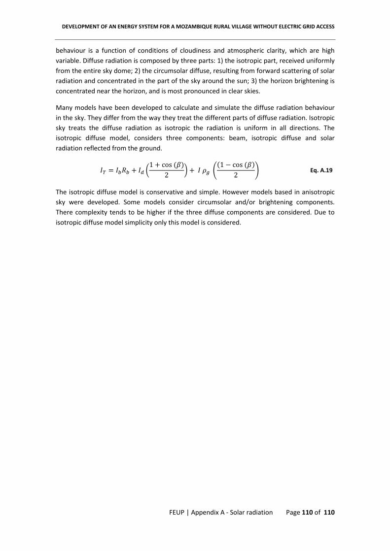
DEVELOPMENT OF AN ENERGY SYSTEM FOR A MOZAMBIQUE RURAL VILLAGE WITHOUT ELECTRIC GRID ACCESS
FEUP | Appendix A - Solar radiation Page 110 of 110
behaviour is a function of conditions of cloudiness and atmospheric clarity, which are high
variable. Diffuse radiation is composed by three parts: 1) the isotropic part, received uniformly
from the entire sky dome; 2) the circumsolar diffuse, resulting from forward scattering of solar
radiation and concentrated in the part of the sky around the sun; 3) the horizon brightening is
concentrated near the horizon, and is most pronounced in clear skies.
Many models have been developed to calculate and simulate the diffuse radiation behaviour
in the sky. They differ from the way they treat the different parts of diffuse radiation. Isotropic
sky treats the diffuse radiation as isotropic the radiation is uniform in all directions. The
isotropic diffuse model, considers three components: beam, isotropic diffuse and solar
radiation reflected from the ground.
�� 8 ��L� h �� o1 h cos f�g2 s h � &� :f1 = cos f�g2 A Eq. A.19
The isotropic diffuse model is conservative and simple. However models based in anisotropic
sky were developed. Some models consider circumsolar and/or brightening components.
There complexity tends to be higher if the three diffuse components are considered. Due to
isotropic diffuse model simplicity only this model is considered.