Development of an active braking controller for brake systems on electric

motor driven vehicles

BENNY TRUONG

Master of Science Thesis MMK 2014:80 MDA 485

KTH Industrial Engineering and Management

Machine Design

SE-100 44 STOCKHOLM

Utveckling av en aktiv broms-regulator för bromssystem på elmotor-drivna fordon

BENNY TRUONG

Master of Science Thesis MMK 2014:80 MDA 485

KTH Industrial Engineering and Management

Machine Design

SE-100 44 STOCKHOLM

i

Abstract

Braking a vehicle can be difficult and the largest braking force is not always the most efficient

braking. A lot of problems occur in case the wheels start to lock up and slide on the road

surface. This is more likely to happen on slippery roads but can happen on high traction roads

as well. When the wheels lose the traction, lock up and start to slide on the road surface the

braking forces between the tyres and the ground are reduced. This results in a longer brake

distance, loss of steering ability and less stability since the tyres lose the major lateral forces.

A new controlled brake system is developed by first creating a system structure with several

subsystems which each solves their tasks to achieve different objectives. The subsystems

developed are the active braking control system, ABC activation system, brake blending

system and dynamical brake torque distribution system. The objective of the controlled brake

system is to reduce the brake distance, achieve regenerated energy and keep the vehicle’s

steering ability.

The master thesis is proposing a controlled brake system for a heavy construction equipment

vehicle. The work is done in cooperation with Volvo Construction Equipment and the

developed system is implemented and tested in a simulation-model for one of company’s

prototype wheel loader. The vehicle used in the thesis is a four-wheel-driven wheel loader

with electric motors in each wheel hub and it has the ability for independent torque actuation

for all individual wheels. The electric motors have the potential to be used as regenerative

brakes where they produce a braking torque and power which can be used to charge a battery.

The braking torque from an electric motor is however limited and not always sufficient, that is

why it needs to be supplemented by friction brakes. The friction brakes are available at each

wheel and are used when the requested braking torque exceeds the torque provided by the

electric motor.

The brake blending strategy distributes the braking torque between electric motors and

friction brakes to achieve regenerative braking. To reduce the brake distance the wheels are

prevented from being locked up and slide. The active braking control system controls the

wheel slip at each wheel to maintain a high friction between the tyre and the ground and

thereby keeping the brake force of the vehicle as high as possible. The vehicle can maintain

the steering ability even during an emergency braking by preventing the wheels from locking

up and thereby keeping the major lateral forces. The wheel slip controller is a PID controller

customized by velocity scaling and output tracking.

The result shows improvements with the new controlled brake system compared to the

conventional brake system used at Volvo CE. The improvements are achieved in aspects of

reduced brake distance, energy regeneration and maintained vehicle steering ability. The

controlled brake system is a novel concept which can be implemented in a prototype vehicle

for development and research purpose. However the system needs further development and

more extensive testing before it can be implemented in a vehicle for the end user since the

brake system is a crucial part of the vehicle and is strongly connected to the safety.

ii

iii

Abstrakt

Att bromsa ett fordon kan vara svårt och den största bromskraften är inte alltid det mest

effektiva sättet att bromsa. Många problem uppstår ifall hjulen börjar låsa sig och glida på

vägbanan, detta är mer sannolikt att hända på hala vägar men kan även hända på vägar med

bra väggrepp. När hjulen förlorar greppet, låser sig och börjar glida på vägbanan minskar

bromskrafterna mellan däcket och marken. Detta resulterar i en längre bromssträcka och

förlust av fordonets styrförmåga och stabilitet eftersom däcken tappar de största sidokrafterna.

Ett nytt reglerat bromssystem utvecklas genom att först skapa en struktur för systemet med

flera delsystem som var och en löser sina uppgifter för att uppnå olika mål. De delsystem som

utvecklas är active braking control systemet, ABC activation systemet, brake blending

systemet och dynamical brake torque distribution systemet. Målet för det reglerade

bromssystemet är att minska bromssträckan, kunna regenerera energi och behålla fordonets

styrbarhet.

Detta examensarbete föreslår ett reglerat bromssystem för tunga anläggningsmaskiner.

Arbetet har skett i samarbete med Volvo Construction Equipment och det utvecklade systemet

implementeras och testas i en simuleringsmodell för ett av företagets prototyp-hjullastare.

Fordonet som används i detta arbete är en fyrhjulsdriven hjullastare med elmotorer i varje hjul

och de har möjligheten till att producera individuella kraftmoment för alla hjul. De elektriska

motorerna kan användas som regenerativa bromsar när de producerar ett bromsmoment

samtidigt som de producerar ström som sedan användas för att ladda ett batteri.

Bromsmomentet från en elektrisk motor är begränsad och inte alltid tillräcklig, därför behöver

de kompletteras med friktionsbromsar. I detta fall finns friktionsbromsar tillgängliga på varje

hjul som används då det begärda bromsmomentet överstiger det vridmoment som levereras av

den elektriska motorn.

Brake blending strategin fördelar bromsmomentet mellan elmotorer och friktionsbromsar för

att uppnå ett regenerativt bromssystem. För att minska bromssträckan hindras hjulen från att

låsa sig och glida. Active braking control systemet styr hjulslirning vid varje hjul för att

bibehålla ett högt väggrepp mellan däcken och marken och därmed hålls bromskraften för

fordonet så högt som möjligt. Fordonet kan upprätthålla styrförmågan även under en

nödbromsning genom att förhindra att hjulen låser sig eftersom de största sidokrafterna

bibehålls. Hjul-slir regulatorn är en PID-regulator anpassad med hastighetsskalning och

utsignalsspårning.

Resultaten visar förbättringar med det nya reglerade bromssystemet jämfört med det

konventionella bromssystemet som används på Volvo CE. Förbättringarna består av minskad

bromssträcka, regenerering av energi och bibehållen styrbarhet på fordonet. Det reglerade

bromssystemet är ett nytt koncept som kan implementeras i ett prototypfordon för

utvecklingssyften och forskningssyften. Systemet behöver vidareutvecklas och kräver mer

omfattande tester innan den kan implementeras i ett fordon för slutanvändaren eftersom

bromssystemet är en viktig del av fordonet och är starkt relaterat till säkerheten.

iv

v

Nomenclature

Notations Symbol Description r Wheel’s radius (m)

L Wheelbase, longitudinal distance from front wheel to rear wheel (m)

Lf Longitudinal distance from front wheel to the center of mass

Lr Longitudinal distance from rear wheel to the center of mass

hg Height of the center of mass from ground (m)

m Vehicle mass (kg)

J Wheel’s moment of inertia (kgm2)

v Longitudinal speed of the vehicle (m/s)

ω Wheel’s angular velocity (rad/s)

Tb Braking torque (Nm)

Fzf Vertical force on the front wheel (N)

Fzr Vertical force on the rear wheel (N)

Fxf Longitudinal force at contact point between front tyre and road (N)

Fxr Longitudinal force at contact point between rear tyre and road (N)

N Vertical load distribution

g Gravitational acceleration (m/s2)

λ Longitudinal wheel slip

µ Longitudinal friction coefficient

a Vehicle’s acceleration

βf Braking force ratio for front wheel

βr Braking force ratio for rear wheel

Abbreviations

ABS Anti-lock Braking System

BBW Brake-By-Wire

IMU Inertial Measurement Unit

ECU Electronic Control Unit

HAB Hydraulic Actuated Brakes

EHB Electro-Hydraulic Brakes

EMB Electro-Mechanical Brakes

SOC State Of Charge

BB Brake Blending

ABC Active Braking Control

DBTD Dynamical Brake Torque Distribution

vi

vii

Table of contents

Abstract ....................................................................................................................................... i

Abstrakt ..................................................................................................................................... iii

Nomenclature ............................................................................................................................. v

Table of contents ...................................................................................................................... vii

List of figures ............................................................................................................................ ix

1 Introduction ......................................................................................................................... 1

1.1 Background ...................................................................................................................... 1

1.2 Description of problems ................................................................................................... 1

1.3 Requirement specifications .............................................................................................. 2

1.4 Methodology .................................................................................................................... 3

1.5 Delimitations .................................................................................................................... 3

2 Frame-of-reference.............................................................................................................. 5

2.1 Vehicle dynamics during a brake ..................................................................................... 5

2.2 Weight transfer dynamics during braking ........................................................................ 8

2.3 Friction brakes ................................................................................................................ 11

2.4 Electrical motor .............................................................................................................. 12

2.5 Brake blending strategies ............................................................................................... 13

2.6 Active braking control .................................................................................................... 15

2.7 ABC activation ............................................................................................................... 16

2.8 Characteristic of the longitudinal wheel slip .................................................................. 17

3 Implementation ................................................................................................................. 19

3.1 Brake system strategy ..................................................................................................... 19

3.2 Brake system structure ................................................................................................... 19

3.3 Dynamical brake torque distribution system .................................................................. 20

3.4 ABC activation system ................................................................................................... 21

3.5 Active braking control system ........................................................................................ 24

3.6 Brake blending system ................................................................................................... 26

3.7 Friction brakes ................................................................................................................ 27

4 Result ................................................................................................................................ 29

4.1 Test procedure and setup ................................................................................................ 29

4.2 Quantitative test .............................................................................................................. 31

4.3 Test case 1 ...................................................................................................................... 39

4.4 Test case 2 ...................................................................................................................... 41

4.5 Test case 3 ...................................................................................................................... 43

4.6 Test case 4 ...................................................................................................................... 47

5 Conclusion ........................................................................................................................ 51

6 Discussion ......................................................................................................................... 53

7 Future work ....................................................................................................................... 55

8 References ......................................................................................................................... 57

Appendix A: Brake system structure........................................................................................ 59

Appendix B: ABC activation system ....................................................................................... 60

Appendix C: Comparison of slipset activation .......................................................................... 61

Appendix D: Comparison of different ................................................................................ 62 Appendix E: Comparison of different wheel slip controllers .................................................. 63

viii

ix

List of figures

Figure 1. A turning wheel loader from Volvo CE where the articulated joint is visible ........... 5

Figure 2. Dynamics for a single wheel motion during braking. ................................................. 6

Figure 3. The friction coefficient as a function of slip ratio and road surface condition

(Savaresi & Tanelli, 2010). ........................................................................................................ 7

Figure 4. Demonstrating the weight transfer where the vehicle is driving on the upper picture

and braking on the lower picture. ............................................................................................... 8

Figure 5. Illustration of the vehicle’s parameters and forces during braking............................. 9

Figure 6. Typical performance characteristics of electric motors for traction (Ehsani, et al.,

2005). ........................................................................................................................................ 13

Figure 7. Illustration of the forces on a one-wheel model (Savaresi & Tanelli, 2010). ........... 17

Figure 8. The dynamical brake torque distribution system with inputs to the left and outputs to

the right of the box. .................................................................................................................. 20

Figure 9. The real-time calculation of the brake torque ratio for the front and rear wheels. ... 21

Figure 10. The ABC Activation system with inputs to the left and outputs to the right of the

box. ........................................................................................................................................... 21

Figure 11. The electric motor’s lookup table for negative torque at the wheel. ...................... 27

Figure 12. A graph of the brake distance data collected in Table 4. ........................................ 32

Figure 13. The brake distance reduced with the new brake system in meters. ........................ 33

Figure 14. Brake distance reduced with the new system in percent......................................... 33

Figure 15. Amount of energy regenerated and dissipated compared. ...................................... 35

Figure 16. Percentage of energy recuperated during the brake tests. ....................................... 35

Figure 17. The use of friction brakes on the new brake system compared to the old system. . 37

Figure 18. wheel slip without ABC, BB and DBTD. ............................................................... 39

Figure 19. Normalized wheelspeed and vehicle speed without ABC, BB and DBTD. ........... 40

Figure 20. Wheel slip with dynamical brake torque distribution. ............................................ 41

Figure 21. Normalized wheelspeed and vehicle speed with only DBTD. ............................... 42

Figure 22. The ABC Activation system shows when the ABC system activates. ................... 43

Figure 23. The wheel slip when ABC and BB is on and DBTD is off. ................................... 44

Figure 24. The normalized wheelspeeds and the vehicle speed with ABC and BB but without

DBTD. ...................................................................................................................................... 44

Figure 25. Shows when the ABC controlled braking is active. ............................................... 47

Figure 26. Wheel slips maintained at 0.2 and never locks during active ABC. ....................... 48

Figure 27. The normalized wheelspeed never drops to zero during braking and thus never

locks. ........................................................................................................................................ 48

Figure 28. Illustration of the brake system structure. ............................................................... 59

Figure 29. The state machine in Simulink of the ABC Activation system. ............................. 60

x

Figure 30. The wheel slip during the braking when the value is 0.2 ......................... 61

Figure 31. The wheel slip during the braking when the value is 0.18 ....................... 61

Figure 32. The wheel slip during the braking when ............................ 62

Figure 33. The wheel slip during the braking when .... 62

Figure 34. The wheel slip during the braking when using a linear PID controller. ................. 63

Figure 35. The wheel slip during the braking when using a PID controller with a nonlinear

slip function. ............................................................................................................................. 63

Figure 36. The wheel slip during the braking when using a velocity-scaling PID-controller. 64

1

1 Introduction

1.1 Background

The brake systems on heavy construction vehicles at Volvo CE have not reached the same

development as on passenger cars. This is probably since heavy construction vehicles do not

reach as high speeds as cars, but instead the construction vehicles are multiple times heavier

than a car and therefore the brake system needs more consideration. It is of great importance

to ensure the safety of heavy construction vehicle and protect the driver, construction workers

and also civilians since these vehicles are often driven at maximum speed when being

transported from one working site to another. These vehicles operate under severe conditions

where the road can be inclined or slippery by water and mud. When the vehicle makes a hard

braking the wheels can lock up and start to slide and this will cause a longer brake distance

and loss of control since the traction is lost. This can occur on the best road conditions but the

consequences are even worse on bad road conditions. Losing the control of these machines is

dangerous considering the massive weight and therefor it is crucial to have top performing

brake systems.

The current construction vehicles manufactured by Volvo CE are only using friction brakes

which are not controlled. The structure is a hydraulic linkage system where the pressure from

the brake pedal propagates to the brakes. The thesis work involves development of a wheel

loader which utilizes electric motors in each wheel to drive the vehicle. This allows for the

opportunity to use the electric motors as generators to brake the vehicle. This additional brake

system contributes to several advantages which improve the system, but the complexity of the

system is increased as well since the motors need to be carefully controlled and constrained to

make sure they are safe and perform as intended. The electric motors are combined with

electro-hydraulic friction brakes which allow for the opportunity to implement a Brake-By-

Wire system which can use controllers and algorithms to achieve a better braking

performance.

1.2 Description of problems

The thesis research question is “Development of an active braking controller for brake

systems on electric motor driven vehicles”.

The thesis is investigating solutions to control the brakes for a heavy construction vehicle.

The vehicle used in the thesis is a four-wheel-driven wheel loader where each wheel is

equipped with an electro-hydraulic friction brake and an electric motor. Both the friction

brakes and the electric motors are producing a braking torque when the vehicle is braking.

The kinetic energy of the vehicle converts into heat and dissipates in the cooling system

during braking with the friction brakes. But the kinetic energy converts into regenerated

electric energy when an electric motor is used to decelerate the vehicle. This energy can be

used to charge an electric storage unit like a battery and later used to drive the vehicle.

Regenerative braking system is an important element in fuel saving of a hybrid electric

vehicle (Tehrani, et al., 2011).

When a vehicle is braking there is something called “weight transfer” which is caused by the

inertial forces of the vehicle. It causes the normal forces to increase on the front wheels and to

2

decrease on the rear wheels. With a static brake torque distribution the wheel loader is equally

distributing the braking force which causes the rear wheels to lock up and slide long before

the front wheels during a hard brake, this happens because the normal load changes. When the

rear wheels lock up first the vehicle gets an unstable motion where it could spin and turn

around. The total braking force is also less since the front wheels can provide with more

braking force when it increases the normal force. Usually it is preferred to have the front

wheels lock first rather than having the rear wheels lock first. It is however best to distribute

the braking force to the wheels according to the weight transfer.

A structure of the brake system is developed where the brakes are controlled to reduce the

brake distance and also achieve regenerated energy during braking. The brake blending

strategy integrates the electric motors with the friction and the system primarily uses the

electric motors to decelerate the vehicle, the friction brakes will be used when the brake force

of the electric motor is insufficient or to hold the vehicle at standstill. Energy regeneration is

achieved by using the electric motors to produce a braking torque.

The benefits of having a brake blending strategy which uses electric motors to brake and

reduces the use of friction brakes are:

Braking energy can be recuperated

The wear of the friction brakes are reduced

The temperature of the friction brakes are reduced which has two advantages o The risk of brake fading is reduced, which occurs when the friction brakes are

overheated

o The cooling system for the friction brakes can be reduced

The active braking control and the dynamical brake torque distribution system are developed

to improve the braking performance by reducing the brake distance, maintaining traction and

steering ability. To achieve a reduced brake distance for the vehicle an active braking control

based on a wheel-slip controller is developed. It applies an individual braking torque

dependent on the traction available at each specific wheel. The benefit with this system is a

shorter brake distance, which means it can stop much faster in case of an emergency situation.

By keeping the traction on all wheels the vehicle will also maintain the lateral forces and

hence it maintains the steering ability during the emergency braking which makes it easier to

avoid obstacles.

The dynamical brake torque distribution system has the objective to counteract the weight

shift dynamic of the vehicle during braking. The benefit of the dynamic torque distribution is

that it makes all the wheels reach the preferred slip value approximately simultaneously. A

more stable braking motion is achieved where the risk of getting a spin on the vehicle is

reduced.

1.3 Requirement specifications

The requirements for the new brake system are:

The brake distance shall be reduced compared to the old brake system

The electric motors shall provide regenerated energy during braking

3

The brakes shall be able to provide the braking torque requested from the new brake

system independently of the electric motor’s limits, e.g., provide enough braking

torque to maintain the reference slip value during the active braking control.

1.4 Methodology

The method to achieve the requirements in chapter “1.3 Requirement specifications” are:

Actively controlling the brake torque on each wheel to increase the brake forces on all wheels individually

Use the electric motors to brake the vehicle by implementing regenerative braking

Through brake blending the friction brakes will be added when the electric motor brake torques are insufficient

A literature study is done on the area of the current state of art and knowledge within the

relevant areas for this research and its technologies. A structure of the brake system is

proposed on how the different components and other logics should be arranged allowing for a

feasible Brake-By-Wire solution. Subsystems are then developed containing strategies for

brake blending, dynamical brake torque distribution and active braking control.

There is no hardware prototype available for a real implementation or hardware in the loop

tests since the wheel loader is a concept under development. Instead the strategies are

implemented in a Simulink-model of the vehicle to perform simulations and test-cases, which

are then evaluated.

1.5 Delimitations

The delimitations of the project are:

Only straight braking is considered and tested, therefore braking in curves is not

included or tested in this thesis.

The physical plant models of the vehicle and brakes are developed and provided by Volvo CE. It is the structure, strategy and all the functions which are developed in this

thesis.

There is no hardware prototype available for a real implementation or hardware in the loop tests since the wheel loader is a concept under development. The system is

instead implemented in a Simulink-model of the vehicle to perform simulations and

test-cases.

It is assumed that the battery never reaches full charge during the tests since the regenerated energy is stored in the batteries. In case the battery is fully charged the

additional energy can be dissipated in brake resistors (Tehrani, et al., 2011). This area

is however not further investigated in this thesis.

The regeneration of energy is the maximum generated energy from the electric motor

and does not consider the ability of charging a specific battery. It proves the potential

of the system’s ability to supply regenerated energy. To get the end result of how

much of the regenerated energy can be stored in a battery one has to make further

investigations of different batteries and strategies to charge them.

4

5

2 Frame-of-reference

2.1 Vehicle dynamics during a brake

The wheel loader has four wheels and the physical structure of the vehicle is very similar to a

car but with dimensions several times larger and heavier than a passenger car. The only

difference of importance related to the intended area is that the wheel loader is an articulated

vehicle. The body of the wheel loader is divided into two parts, one front unit and one rear

unit. The rear wheels are attached to the rear unit and the front wheels are attached to the front

unit. These two parts are connected with an articulated joint and the vehicle pivots at the joint

whenever the wheel loader is turning. The wheels are never turning sideways in relation to

their respective unit.

Figure 1. A turning wheel loader from Volvo CE where the articulated joint is visible

This might induce a slightly different turning behavior but since only straight braking is

considered and simulated the articulating joint does not affect the results and therefore most

of the vehicle dynamics that apply to cars are also applicable to the wheel loader in this thesis.

The vehicle dynamics can be described by Newton’s second law and hence the deceleration of

a vehicle during braking can be described as following. Figure 5 shows an illustration of the

forces.

( ) (2.1)

where is the vehicle’s total mass,

is the acceleration and , are the longitudinal

brake forces at the contact point between the tyre and the ground for the front wheel

respectively the rear wheel. The angular dynamics for a single wheel motion can be described

as following. Figure 2 shows an illustration of the equation.

(2.2)

6

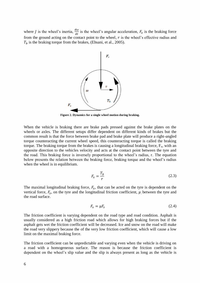
where is the wheel’s inertia,

is the wheel’s angular acceleration, is the braking force

from the ground acting on the contact point to the wheel, is the wheel’s effective radius and

is the braking torque from the brakes, (Ehsani, et al., 2005).

Figure 2. Dynamics for a single wheel motion during braking.

When the vehicle is braking there are brake pads pressed against the brake plates on the

wheels or axles. The different setups differ dependent on different kinds of brakes but the

common result is that the force between brake pad and brake plate will produce a right-angled

torque counteracting the current wheel speed, this counteracting torque is called the braking

torque. The braking torque from the brakes is causing a longitudinal braking force, Fx, with an

opposite direction to the vehicles velocity and acts at the contact point between the tyre and

the road. This braking force is inversely proportional to the wheel’s radius, r. The equation

below presents the relation between the braking force, braking torque and the wheel’s radius

when the wheel is in equilibrium.

(2.3)

The maximal longitudinal braking force, , that can be acted on the tyre is dependent on the

vertical force, , on the tyre and the longitudinal friction coefficient, µ, between the tyre and the road surface.

(2.4)

The friction coefficient is varying dependent on the road type and road condition. Asphalt is

usually considered as a high friction road which allows for high braking forces but if the

asphalt gets wet the friction coefficient will be decreased. Ice and snow on the road will make

the road very slippery because the of the very low friction coefficient, which will cause a low

limit on the maximal braking force.

The friction coefficient can be unpredictable and varying even when the vehicle is driving on

a road with a homogeneous surface. The reason is because the friction coefficient is

dependent on the wheel’s slip value and the slip is always present as long as the vehicle is

7

braking. The wheel’s longitudinal slip value is often calculated as a ratio which is the

normalized relative velocity between the tyre and the road (Savaresi & Tanelli, 2010). Since

only the straight forward braking is considered in this thesis the tyre sideslip angle is zero and

hence the longitudinal wheel slip is following.

(2.5)

Figure 3 below shows how the friction coefficient is dependent on the road surface condition

and varies with the longitudinal slip ratio. The friction coefficient for each road is also

strongly dependent on the tyre’s rubber and tread. Therefore the magnitude of the data in

Figure 3 can be seen as an approximate but the main purpose is to show the characteristics of

how the friction coefficient varies with different roads and slips. An important observation is

how the friction coefficient has a maximum peak value at a certain slip before it starts to drop

again for increasing slip values.

Figure 3. The friction coefficient as a function of slip ratio and road surface condition (Savaresi & Tanelli, 2010).

A high friction coefficient allows for high braking forces for a specific load on the wheels and

therefore a high friction coefficient is desirable. As pointed out there is a peak value of the

friction coefficient for a certain slip point where the friction coefficient is steadily decreasing

beyond that slip point. The goal is to aim for a certain slip value where the friction coefficient

is at its maximum value, this allows for a high braking force. As seen in Figure 3, there is no

single optimal longitudinal slip which suits all road surface conditions.

The ideal longitudinal slip is considered to be at 0.2 to get the maximum braking force on the

wheels. 0.2 in slip value corresponds to a 20 % speed difference between the normalized

wheel speed and the ground. A wheel slip of 0.2 is approximately close to the average of the

different maximum friction values for the roads. Using 0.2 as the preferred longitudinal slip is

8

very common and has also been recognized and used by (Ehsani, et al., 2005), (Tehrani, et al.,

2011) and (Savaresi & Tanelli, 2010) among others in their work and that is the reason for

choosing the slip value of 0.2.

2.2 Weight transfer dynamics during braking

During braking the inertial force of the vehicle’s mass is contributing to a weight transfer

(Mutoh, et al., April 2007) which affects the normal force on each wheel. The weight transfer

increases the normal forces on the front wheels and decreases the normal force on the rear

wheels by the same amount. Figure 4 demonstrates the weight transfer. The cause of this

phenomenon is because the vehicle’s center of gravity has a certain height from the ground

and the brake forces are acting on the contact points between the wheels and the ground. The

height on the center of gravity point becomes the lever and thus the weight shift becomes

stronger when the center of gravity is increasing in height.

Figure 4. Demonstrating the weight transfer where the vehicle is driving on the upper picture and braking on the

lower picture.

9

If the distribution ratio of the brake torques to the front and rear wheels are static the front

wheels will start to slip much earlier than the rear wheels because of the weight transfer.

Whether it is the front or rear wheels that starts to slip depends on the actual distributed ratio.

When the ratio is 50 % the brake torque distribution to the front and rear wheels are equal and

the consequence is that the rear wheels will start to slip earlier than expected because of the

decreased normal force on the rear wheels. If there is no ABS system the rear wheels will lock

entirely and the vehicle will lose the lateral stability.

A vehicle with the front wheels locked and the rear wheels still rolling will have a stable

straight-ahead motion but without steering ability. If the rear wheels are locked and the front

wheels are still rolling the vehicle will get an unstable motion where the vehicle spins and

turns around. Usually it is preferred that the front wheels lock first rather than having the rear

wheels lock first (Jacobson, 2011).

Figure 5 shows the forces during braking and the load for the front wheel can be found by

calculating the moment equation on the rear wheel at the contact point to the ground

according to (2.6) (Jacobson, 2011). The vehicle suspension is considered to be stiff in the

mathematical equations for the vehicle dynamics.

Figure 5. Illustration of the vehicle’s parameters and forces during braking.

(2.6)

where is the normal force on the front wheel, is the wheelbase, m is the vehicle’s mass,

g is the gravitational acceleration, is the longitudinal distance between the center of gravity

to the center of the rear wheel, is the inertial force when braking and the is the

10

center of gravity’s height. Since the vehicle is braking the acceleration is negative and thus

the force from the inertia is following.

( ) (2.7)

By combining (2.6) and (2.7) the normal forces can be calculated on the front and rear wheels,

Fzf and Fzr. They are varying dependent on the vehicle’s mass, deceleration of the vehicle and

the location of the vehicle’s center of gravity point. The total normal force on the front axle

can be expressed as following (Ehsani, et al., 2005).

(

) (2.8)

To find the normal force on the rear wheel the same procedure can be done but the moment

equation in (2.6) needs to be calculated at the contact point between the front wheel and the

ground instead of the rear wheel.

(

) (2.9)

With (2.4) the normal force can be translated to the longitudinal maximal braking force for

the front and rear wheels, Fxf and Fxr

(

(

)) (2.10)

and

(

(

)) (2.11)

According to an investigation done on an electric vehicle with independently driven front and

rear wheels, (Mutoh, et al., April 2007), the weight transfer compensation successfully

prevents the rear wheels from locking up long before the front wheels. The study considers

the weight transfer dynamic and counteracts it by reducing the amount of brake torques to the

rear wheels and increases the braking torque to the front wheels. All the wheels will then

reach the maximal braking force simultaneously and thereby the vehicle will brake in an

efficient way and it keeps the stability as long as possible. If the braking forces exceed the

maximal braking force the wheels would start to slip simultaneously.

The load transfer estimation is done with acceleration and friction coefficient as signal inputs.

The acceleration can easily be measured by an inertial measurement unit which is mounted

close to the center of the vehicle’s mass. The friction coefficient is however an unknown

parameter which depends on the road surface condition and changes continuously. To be

independent of the friction coefficient a ratio calculation is done, βf and βr, for the distribution

11

of the total braking force to the front and rear wheels’ braking forces (Mutoh, et al., April

2007). The front axle’s normal force ratio varies as following.

(2.12)

(2.13)

and since βf and βr are ratios, the sum of them is 1. The rear wheels’ ratio can simply be

calculated as following.

(2.14)

of course the complete calculation for the rear axle’s ratio can be calculated in the same

procedure as following.

(2.15)

(2.16)

Observing the equations for the ratios it can be noticed that the calculation only needs the

acceleration signal as an input. The ratios are multiplied with the total requested braking force

of vehicle to get the proper amount of braking force distributed to the front and rear wheels.

(2.17)

and

(2.18)

where Fx is the braking force acting on the wheel, β is the brake ratio and Fbrake demand is the

total requested braking force for the vehicle.

2.3 Friction brakes

There are three different systems of braking actuators when it comes to friction brakes,

hydraulic, electro-hydraulic and electro-mechanical (Savaresi & Tanelli, 2010). The hydraulic

12

actuating brakes are the conventional brakes and most commonly used in passenger cars. The

pressure on the brake pedal is transmitted to the hydraulic system directly through valves,

pumps and accumulators. Since the force is transferred directly through the brake fluid, the

control of brake force is strongly limited. Vehicles using hydraulic actuators combined with

ABS are usually considered to have a discrete force modulation because of the large pressure

gradient in the hydraulic circuit, which makes the brake to alternate between on and off in a

fast pace causing hard vibrations. Because of the physical direct linkage between the brake

pedal and the brake pads, the hydraulic pressure applied to the brakes cannot be bypassed.

Electro-hydraulic actuating brakes provide a force feedback similar to hydraulic actuators at

the brake pedal but instead of having a direct connection all the way to the brake pads, the

pedal position is measured and electronically transferred to a hydraulic unit with an electronic

control unit (ECU). From there the ECU transfers the signal and actuates the brake through

hydraulic fluid.

The electro-mechanical actuating brakes are similar to the electric-hydraulic brakes but it is

entirely mechanical and thus it is a dry system instead of using hydraulic fluid to transfer the

brake force.

The two electronically driven actuators don’t have direct connection between the brake pedal

and the brake unit which allows for a continuous force modulation, all this contributes to a

much better control of the brake forces. The hard vibrations experienced with the hydraulic

actuating brakes no longer exists (Savaresi & Tanelli, 2010).

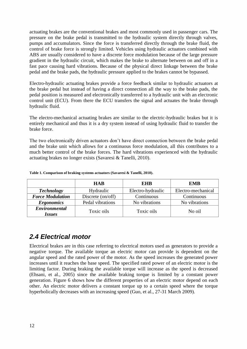
Table 1. Comparison of braking systems actuators (Savaresi & Tanelli, 2010).

HAB EHB EMB

Technology Hydraulic Electro-hydraulic Electro-mechanical

Force Modulation Discrete (on/off) Continuous Continuous

Ergonomics Pedal vibrations No vibrations No vibrations

Environmental

Issues Toxic oils Toxic oils No oil

2.4 Electrical motor

Electrical brakes are in this case referring to electrical motors used as generators to provide a

negative torque. The available torque an electric motor can provide is dependent on the

angular speed and the rated power of the motor. As the speed increases the generated power

increases until it reaches the base speed. The specified rated power of an electric motor is the

limiting factor. During braking the available torque will increase as the speed is decreased

(Ehsani, et al., 2005) since the available braking torque is limited by a constant power

generation. Figure 6 shows how the different properties of an electric motor depend on each

other. An electric motor delivers a constant torque up to a certain speed where the torque

hyperbolically decreases with an increasing speed (Guo, et al., 27-31 March 2009).

13

Figure 6. Typical performance characteristics of electric motors for traction (Ehsani, et al., 2005).

The braking torque from electric motors need to be controlled when used as regenerative

brakes since the braking torque is a torque in the opposite direction of the wheel speed. If the

magnitude of the negative torque exceeds the magnitude of the maximal braking force as

explained in equation (2.4) the wheels would start to spin backwards while the vehicle is still

sliding forward. Locked wheels does not only increase the brake distance but it also lowers

the regenerated energy since the rotational speed is close to zero when the wheels are locked

and the power regeneration is proportional to the rotational speed (Tehrani, et al., 2011).

The friction brake provides the remaining torques in case the available torque from the

electric motor is lower than the total requested torque. During braking the available torque

from the electric motors increases as the speed of the electric motor decreases and thus the

torque from the friction brake should gradually decrease to maintain the correct total braking

torque.

During braking the electric motors turns the kinetic energy into electrical energy, thus it

regenerates power. This power can charge a battery according to its limitations and free

capacity. Additional energy can be dissipated in brake resistors (Tehrani, et al., 2011). During

standstill the electrical motors can’t provide with a braking torque, hence the friction brakes

are used when holding the vehicle during standstill.

2.5 Brake blending strategies

Brake blending is the strategy to distribute the total brake torque between the electric motors

and the friction brakes. The most common goals are to regenerate maximal amount of energy

with electric motors but the vehicle dynamics and braking technologies capabilities are the

main constraints. Most studies are done on cars with regenerative brakes only available on

one axle and electric motors are usually insufficient at providing enough braking torque. This

is the reason for many brake blending strategies where the friction brakes are always in use.

Braking with only one axle induces unstable dynamics on the vehicle and is not the most

optimal way of braking. Therefore several studies have been done on how to optimize the

brake blending control with some optimization techniques with the objectives of maximizing

the regenerated energy with the constraints of keeping the vehicle stability and maintain a safe

braking.

14

(Falcone, et al., 15-18 December 2009) present two model predictive approaches for

controlling the regenerative braking at the rear axle in cornering maneuvers where they

consider yaw movements as well. The study is focusing on the cornering characteristics of the

vehicle.

(Guo, et al., 27-31 March 2009) have done a study on braking force distribution by optimizing

it through genetic algorithms. The optimization process is a probabilistic global search that

mimics the metaphor of natural biological evolution.

(Cao, et al., 2-5 July 2008) have combined the technique of sliding mode control and neural

network identification. It utilizes the sliding mode control to control the brakes and to

optimize the process the neural network technique is used to do on-line parameter adjustment

and system identification to achieve self-learning, self-adapting and self-organization.

Different fuzzy controllers have been developed and they have the ability to convert the

linguistic expressions into an automated fuzzy rules based control strategy. They are however

experiencing difficulties to guarantee stability and robustness of the system (Kim & Lee, 12

May 1995). This is why different combinations have been implemented such as fuzzy sliding-

mode control (Kim & Lee, 12 May 1995) which is more robust against parameter variation.

The major drawbacks about fuzzy rules are that they require previously tuned rules by time-

consuming trial-and-error procedures (Lin & Hsu, March 2003).

Some vehicles are found with individual torque distribution on each wheel which has

regenerative brakes and friction brakes on each wheel. These vehicles have the advantage of

having regenerative brakes available at all wheels and the potential to regenerate energy is

bigger. The regenerative brakes don’t have to be blended with friction brakes at all times in

order to get an optimal torque distribution and achieve a stable vehicle dynamic. Instead the

brake blending’s most obvious purpose is to make sure the total braking torque is correct by

blending with the friction brakes when the electric motors no longer can provide enough

braking torque. The most common way to achieve this is to use a method called control

allocation.

(Shyrokau, et al., 2013) use a multi-layer vehicle controller with an optimization-based

control allocation method to achieve vehicle dynamics control and energy recuperation for a

car. The brake blending algorithm is a weighting matrix which depends on normal forces,

vehicle motion and recuperation algorithms based on thresholds of the battery’s and electric

motor’s physical conditions.

(Shyrokau, et al., June 2013) is a work from the same authors above with one additional

author and this work has implemented the same technique introduced in (Shyrokau, et al.,

2013) . A multiple level control system is used with a vehicle dynamics control and an

optimized control allocation which is based on a weighting strategy that considers actuators

and tyre friction constraints. They are using multi-objective formulation of independent cost

functions to reach optimal characteristics of vehicle motion and energy consumptions. The

brake blending is focused on recuperation of energy and tyre energy dissipation.

Both these work are based on the same technique overall but the latter one is an offline

optimization method which means they are calculating the optimal brake blending ratio based

on the optimization algorithm on some simulations and this brake blending ratio will then be

used as a static value. They are covering the energy efficiency but are more focused on

15

keeping the steering and vehicle stability, they are creating a solution for an over-actuated

system for commercial cars. The brake distance and energy regeneration is not the main sole

issue. Looking at the optimization constraints in the control allocation technique used in

(Shyrokau, et al., 2013) it can be noticed that the use of regenerative brakes are optimized

against the electric motor’s angular speed, temperature, SOC, vehicle velocity, battery’s

voltage and fault indication.

The total regenerated energies are not comparable since the studies referred above are not

using the same test-cases. The first five references mentioned in this chapter are using more

complex brake blending strategies which are focused on the procedure of optimizing the

energy recuperation and vehicle stability. Mostly the setups only have regenerative braking on

one axle which means the friction brakes are always used during braking since all wheels are

preferred to generate a braking torque. This is a challenging factor since the regenerative

braking is less efficient compared to only using regenerative braking on all wheels. The two

last mentioned references are based on a more hardware focused viewpoint where

regenerative braking exists on all wheels. The optimization is not as complex as the rest. The

structure is simple yet effective and the work is implementing a brake blending strategy in a

more complete braking solution which considers most of the vehicle dynamics.

2.6 Active braking control

The active braking control (ABC) system controls the amount of total requested braking

torque on each individual wheel to achieve the highest braking force as possible. The braking

force between the tyre and the ground increases as the braking torque increases until the

wheel is locking up and the tyre will then start to slide on the ground. It is well known that the

tractive force is decreased when the wheels lock up and slide. Not only is the braking distance

increased when the wheels are locking up but the steering ability becomes bad as well since

the lateral forces are decreased. To achieve the maximal braking force the braking torque

needs to be at its maximum without exceeding the value where the wheel is locking up and

the tyre starts to slide.

This has also been known as an anti-lock braking system (ABS) which has the same purpose

as ABC. The difference between the traditional ABS system and the more modern ABC

system is that the standard ABS system is usually equipped with traditional hydraulic

actuators which mainly uses rule-based control logics with discrete modulation of the braking

torque while modern ABC systems uses electro-hydraulic or electro-mechanical actuators

which allows for a continuous modulation of the braking torque (Savaresi & Tanelli, 2010).

The result is that the ABC systems can be treated as a classical regulation problem where the

wheel slip can be controlled and maintained at a certain slip value with higher accuracy and

better result.

In braking control systems, two output variables are usually considered for regulation

purposes; wheel deceleration and wheel longitudinal slip. The traditional controlled variable,

which is still used in some ABS systems, is the wheel deceleration. This is due to the fact that

it can be easily measured with a simple wheel encoder. However the dynamics of a classical

regulation loop on the wheel deceleration critically depends on the road conditions and can

cause problems if road surface changes rapidly. Henceforth deceleration-based control

strategies inherently require the online estimation of the road characteristics. Furthermore the

deceleration control is usually not implemented as a classical regulation loop but instead

heuristic threshold-based rules are used (Savaresi & Tanelli, 2010).

16

On the other hand, the regulation of the wheel slip is very robust from the dynamical point of

view, which means it can handle road surface variations better. But the slip measurement is

critical since it requires the estimation of the speed of the vehicle. Noise sensitivity of slip

control is a critical issue. The major flaw of slip control is that the measurement of the wheel

slip is comparatively difficult and unreliable, especially at low speed. The sensitivity of wheel

slip control to measurement errors is a key issue. (Savaresi & Tanelli, 2010)

(Lin, et al., 24 November 1993) develops a sliding mode control which is a robust nonlinear

control design. The goal is to contain the system in a sliding surface plane where a predefined

function of error is zero. Neural network control has been developed and is a method for

nonlinear mapping between the input-output. The neural network consists of interconnected

neurons which does a nonlinear transformation to the received signals. However it needs

learning and training processes. Fuzzy logic control has also been researched but tuning a

fuzzy logic controller requires experience and consists of trial and error procedure. It is rather

time-consuming and specifically adapted to one type of a vehicle.

The challenge when controlling the slip is that the relation between the slip and the friction

coefficient is nonlinear. A typical PID-controller is linear and therefor the ability to control

the slip with a linear PID controller is limited. However there are methods to customize the

PID-controller for it to become nonlinear, three alternatives are considered.

PID-controller with a nonlinear slip function

Friction-scheduled PID-controller

Velocity-scaling PID-controller

(Solyom, June 2002) uses a velocity-scaling PI controller with gain scheduling to control the

wheel slip. The scheduling is based on the slip and an estimated friction coefficient. The

solution is simple with limitations but powerful and less resource demanding on hardware.

The estimations for the friction coefficient and the vehicle speed are done by a Multi-Model

Observer integrated in the simulator.

(Jiang, 2000) proposes a cascaded control structure for ABS where he implements three

different controllers; a linear PID controller, robust controllers using loop-shaping method

and a nonlinear slip function PID controller. The PID controller is simple but has sensitivity

problems although it achieves satisfactory results. The robust controller is more effective but

is hard and time-consuming to tune. The nonlinear slip function PID controller is getting

better results than a linear PID controller but still maintains the easy tuning advantage.

2.7 ABC activation

The first step towards implementing an active braking control system is to be able to detect

when it should be active and not active. The braking system has two modes; emergency

braking and normal braking. The driver has to be able to control the braking torque during a

normal, non-critical braking but if the driver is making an emergency braking the active

braking control system needs to detect the situation in order to activate and automatically

control the brakes. There has to be logics which sense the switch between manual and

automatic braking mode. (Savaresi & Tanelli, 2010)

17

2.8 Characteristic of the longitudinal wheel slip

By simplifying the vehicle model into a one-wheel model the behavior of the longitudinal

wheel slip can be analyzed in a more easy way.

Figure 7. Illustration of the forces on a one-wheel model (Savaresi & Tanelli, 2010).

From the one wheel model in Figure 7 the following dynamic equations can be acquired

which describes the wheel’s angular and longitudinal motion (Savaresi & Tanelli, 2010).

{

(2.19)

The relation between the vertical force and the longitudinal brake force on the wheel is

according to below.

(2.20)

(2.20) can be substituted in (2.19) which will result in following.

{

(2.21)

Recall below the equation for wheel slip, λ, which is defined as the difference of the

longitudinal speed between the ground and the wheel at their contact point.

(2.22)

where v is the vehicle speed, r is the wheel’s effective rolling radius and is the wheel’s

angular speed. (2.22) can also can be written in two further ways.

( ) (2.23)

(2.24)

by deriving (2.24) with time one will get.

18

(2.25)

The first equation in (2.21) can change the state variable from to since they are linked with the relation in (2.22), (Savaresi & Tanelli, 2010). This is done by substituting (2.23) and

(2.25) into the first equation in (2.21). The dynamic equations will then become.

{

(( )

)

(2.26)

The longitudinal dynamics of the vehicle is much slower than the rotational dynamics because

of the difference of inertia in the wheel compared to the whole vehicle. This makes it

reasonable to neglect the second equation in (2.26) and thereby the equation of the system

becomes a first order model of the wheel slip dynamics. Thus rewriting the first equation of

(2.26) one gets.

( )

(2.27)

Equation (2.27) will be used later in the implementation part to motivate the choice of

controller.

19

3 Implementation

3.1 Brake system strategy

The requested brake torque is decided by the driver’s pressure on the brake pedal during

normal braking. The brake system dynamically distributes the brake torques to match the

individual normal forces on each wheel based on the vehicle’s deceleration to compensate for

the weight transfer. When an emergency braking is detected by the ABC activation system the

ABC system will take over the control of the brakes and provides an automatic braking

torque. It increases the braking torque but still maintains the wheel’s traction and thereby the

vehicle gets a shorter braking distance without losing the vehicle stability and steering ability.

The purpose of the brake blending system is to provide with regenerated energy from the

electric motors and it is done based on the wheel speed. Thereby the brake blending system is

active on both normal braking and emergency braking. The electric motors themselves are

insufficient as the only brake system and thus the friction brakes provides with additional

braking torque to guarantee that the total braking torque is corresponding to the requested

brake torque.

The brake system strategies when the vehicle is braking are:

To dynamically distribute the total brake demand from the pedal based on the acceleration to compensate for the weight transfer.

Apply the required brake torque at each wheel with electric motor brakes.

Blend in the friction brake to satisfy the requested brake torque if the electrical motor brake torque is less than the requested brake torque.

If emergency braking is detected, switch from manual braking to active braking control.

3.2 Brake system structure

The brake system is structured into sub-systems consisting of ABC activation system, active

braking control system, dynamical brake torque distribution system, brake blending system

and the individual brakes. See Appendix A for a flowchart illustration of the structure. Every

subsystem has a specific task and purpose with simple inputs and outputs.

When the brake pedal is pressed by the driver there are two ways the signal can propagate

through the brake system. During normal braking the driver controls the brakes manually, this

means the brake pedal is acting as a feed forward system where the vehicle is braking

according to the driver’s manual request i.e. the brake pedal actuation. In manual braking the

dynamical brake torque distribution makes sure to provide the proper amount of braking

torque to the front and rear wheels based on the vehicle’s deceleration to compensate for the

weight transfer. The second path is the active braking control system which applies an

automatically controlled brake torque on each individual wheel to increase the brake forces

without locking up the wheels. The ABC activation system decides if the actual braking is an

emergency braking or normal braking and will then decide if the manual braking torque is to

be used or the active braking control system should override the driver’s braking request. The

brake blending system contains the strategy of mixing the regenerative braking with the

20

friction braking. The individual brakes are the electric motor brake and the controlled friction

brake.

3.3 Dynamical brake torque distribution system

The braking is manually controlled by the driver through the brake pedal during a non-

emergency braking. The driver controls the total braking torque but the distribution of the

brake torque to the front and rear wheels will be dynamic based on the vehicle’s deceleration

according to the chapter “2.2 Weight transfer dynamics during braking”. By dynamically

distributing the brake torque to the front and rear wheels the vehicle can increase the total

braking torque and prevent the rear wheels from locking up before the front wheels, thereby

the risk of getting an unstable motion where the vehicle spins and turns around is reduced.

The rear wheels saturate sooner than the front wheels when a static ratio is used for

distributing the brake torque. The rear wheels will start to slide while the front wheels are still

rolling and could provide additional braking torques. Thus the risk of getting an unstable

motion where the vehicle spins around is increased when using a static brake torque

distribution.

The system gets a brake pedal signal and a predefined brake torque value to identify the

requested manual brake torque for the vehicle. The brake pedal decides how much of the

predefined brake torque to request. The brake pedal value ranges from 0 to 1 which is

multiplied with the predefined brake torque. A fully pressed brake pedal corresponds to 1 and

a fully released brake pedal corresponds to 0.

The system receives the total torque request from the driver and calculates the brake torque

ratio to the front and rear wheels with the vehicle acceleration signal from the inertial

measurement unit on the vehicle. The system then outputs the brake torque request to the

front and rear wheels which counteract the weight transfer during braking.

Figure 8. The dynamical brake torque distribution system with inputs to the left and outputs to the right of the box.

The system only needs the acceleration as a real-time input signal. The remaining parameters

used in the calculation are static geometrical values like the wheelbase, the center of gravity’s

height and the longitudinal distance from the center of gravity to the rear wheel axle. The

center of gravity’s height is the most difficult parameter to measure and is therefore tuned

through simulations to find the appropriate value. The center of gravity’s height is found

where both the front and rear wheels are approximately locking simultaneously without the

ABC system. The important thing is to make sure the wheels either lock simultaneously or

having the front wheels lock slightly before the rear wheels since this is preferred (Jacobson,

2011).

21

Figure 9. The real-time calculation of the brake torque ratio for the front and rear wheels.

Equation (2.13) and (2.14) is implemented in Figure 9 and that is how the dynamical brake

torque distribution system distributes the brake torques to the front and rear wheels.

3.4 ABC activation system

The ABC activation recognizes whether the braking is an emergency braking or normal

braking and it will switch between manual braking and automatic braking according to

different conditions. The ABC activation system is developed as a state machine in Simulink.

Figure 10 shows the system’s input and output, an illustration of the state machine can be

found in Appendix B: ABC activation system.

Figure 10. The ABC Activation system with inputs to the left and outputs to the right of the box.

The ABC activation system has two modes; ABC ON and ABC OFF. The active braking

control system is automatically controlling the brake torque during ABC ON and the driver is

manually braking during ABC OFF. Within each of the two modes there are two states which

are separated by the speed of the vehicle since the controlled braking gets unreliable and less

necessary when the vehicle is moving in a slow speed.

When the ABC is off the torque is manually controlled through the brake pedal no matter if

the vehicle speed is high or low. But the ABC system can only be turned on when the vehicle

is moving in high speed. The ABC system uses the last manual braking torque value when it

activates and starts to compensate from that value. The last braking torque is maintained as a

static value when the vehicle reaches a very low speed during ABC ON mode until the ABC

22

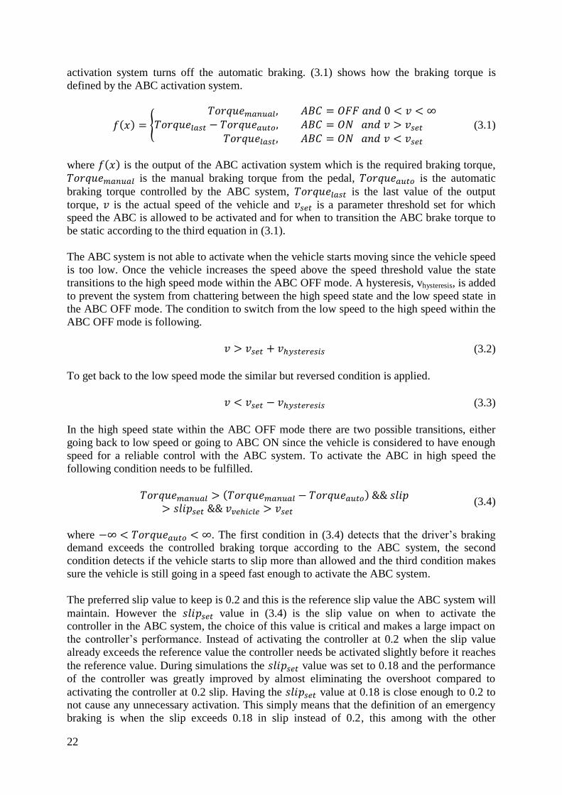
activation system turns off the automatic braking. (3.1) shows how the braking torque is

defined by the ABC activation system.

( ) {

(3.1)

where ( ) is the output of the ABC activation system which is the required braking torque,

is the manual braking torque from the pedal, is the automatic

braking torque controlled by the ABC system, is the last value of the output

torque, is the actual speed of the vehicle and is a parameter threshold set for which speed the ABC is allowed to be activated and for when to transition the ABC brake torque to

be static according to the third equation in (3.1).

The ABC system is not able to activate when the vehicle starts moving since the vehicle speed

is too low. Once the vehicle increases the speed above the speed threshold value the state

transitions to the high speed mode within the ABC OFF mode. A hysteresis, vhysteresis, is added

to prevent the system from chattering between the high speed state and the low speed state in

the ABC OFF mode. The condition to switch from the low speed to the high speed within the

ABC OFF mode is following.

(3.2)

To get back to the low speed mode the similar but reversed condition is applied.

(3.3)

In the high speed state within the ABC OFF mode there are two possible transitions, either

going back to low speed or going to ABC ON since the vehicle is considered to have enough

speed for a reliable control with the ABC system. To activate the ABC in high speed the

following condition needs to be fulfilled.

( )

(3.4)

where . The first condition in (3.4) detects that the driver’s braking demand exceeds the controlled braking torque according to the ABC system, the second

condition detects if the vehicle starts to slip more than allowed and the third condition makes

sure the vehicle is still going in a speed fast enough to activate the ABC system.

The preferred slip value to keep is 0.2 and this is the reference slip value the ABC system will

maintain. However the value in (3.4) is the slip value on when to activate the controller in the ABC system, the choice of this value is critical and makes a large impact on

the controller’s performance. Instead of activating the controller at 0.2 when the slip value

already exceeds the reference value the controller needs be activated slightly before it reaches

the reference value. During simulations the value was set to 0.18 and the performance

of the controller was greatly improved by almost eliminating the overshoot compared to

activating the controller at 0.2 slip. Having the value at 0.18 is close enough to 0.2 to not cause any unnecessary activation. This simply means that the definition of an emergency

braking is when the slip exceeds 0.18 in slip instead of 0.2, this among with the other

23

conditions in (3.4). The results of a test case, as described in chapter “4.1 Test procedure and

setup”, when the value is set to 0.2 and 0.18 are presented in “Appendix C:

Comparison of slipset activation”. The choice of activating the ABC at 0.18 slip is reasonable

and have been implemented by others. (Tehrani, et al., 2011) uses 0.18 slip as a threshold

where the manual braking is applied when the slip value is 0.18 or less. When the slip value

exceeds 0.18 slip the controller decreases the braking torque.

Once the ABC activates in high speed mode the output brake torque is according to the

second equation in (3.1), it uses the last manual brake torque value and controls it by

subtracting the last manual brake torque with the controlled brake torque. The output brake

torque is the sum of both values. The controlled brake torque is a customized PID controller

which will be more detailed described in the chapter about the ABC system.

It is possible to make the output brake torque just a value of the controlled brake torque

without including the last manual brake torque value as following.

( ) (3.5)

This approach works with almost the same result, the difference is that the output value might

start being controlled from a starting value further away from the last used manual braking

torque output. This causes the transition to be larger than necessary when going from the

manual brake torque to the controlled brake torque. Instead the output controlled brake torque

used is in (3.1) but is repeated for the purpose of easier understanding.

( ) (3.6)

A comparison was made which confirmed that (3.6) gave better results than (3.5) where the

step response was more stable with a faster settling time and with less overshoot. (3.6) is the

chosen to be implemented since it gave the best performance. The comparison made between

(3.5) and (3.6) were using a test case described in “4.1 Test procedure and setup” and the

results are presented in “Appendix D: Comparison of different ( )”.

The ABC system requires the driver to keep the brake pedal pushed down to maintain active.

The system will end the braking if the driver releases the brake pedal and thus the ABC

activation system will check for this action. When the following condition is fulfilled the

ABC system turns off and transitions back to the high speed state in ABC OFF mode.

(3.7)

An important issue in this area is to make sure that the system does not chatter between two

different states. Therefore the conditions need to be carefully designed with decent margins to

reduce the risk of unintended switching between two different states.

The state transitions to the low speed state within the ABC ON mode when the ABC system

has effectively reduced the vehicle speed to a certain value. The vehicle speed is slow enough

to switch the controlled braking torque off and replace the output brake torque with the last

brake torque value as a static output. An alternative here is to take the last output brake torque

and gradually reduce the braking torque output to get a smoother end of the braking.

24

At the low speed state in the ABC ON mode the system checks for a released brake pedal or a

vehicle speed below the threshold, , in which case it will return the control of the brakes

back to the driver by transitioning to the low speed state in ABC OFF mode as following.

| | (3.8)

3.5 Active braking control system

The ABC system controls the amount of total requested braking torque on each individual

wheel to achieve the highest braking force as possible. The controller’s input is the wheel slip

and output is the torque. There is one controller for each wheel making it possible for the

system to control each wheel individually.

A simple controller with the ability for easy tuning is preferable and a PID controller is

considered to fulfill these requirements, furthermore Volvo CE desires an investigation of

such a controller. A linear PID controller is studied and implemented but unsatisfactory

results are obtained due to the braking characteristics being a nonlinear behavior. The

vehicle’s velocity, wheels’ slip and road friction coefficient are all nonlinear and this is

causing the braking characteristic to be nonlinear. The best controller would counteract all

three nonlinearities but such a controller would be too complex and therefore three different

gain-scheduled PID controllers are considered where each controller counteracts one of the

mentioned nonlinearity. The preferable controller is the one that achieves the best overall

performance despite only counteracting one of the mentioned nonlinearity. The three

nonlinear gain-scheduled PID controllers are:

Velocity-scaling PID controller

PID controller with a nonlinear slip function

Friction-scheduled PID controller

There has to be an appropriate scheduling variable in order to implement a gain-scheduled

PID controller (Lingman, 2005). The friction coefficient is a suitable scheduling variable.

(Solyom, June 2002) uses the maximum friction coefficient as one of the scheduling variables

which is being estimated. The friction coefficient needs to be estimated to achieve the surface

identification and since no such estimation is included in the thesis the friction-scheduled PID

controller is not further investigated or implemented.

The PID controller with a nonlinear slip function is defined as (Jiang, 2000).

( ) ( ( ) ) (∫ ( ) ) (

( ) ) (3.9)

( ) is a nonlinear function where is ( ) and ( ) is the wheel’s slip. The nonlinear slip function is defined as.

( ) {

( )| | | |

| | (3.10)

25

where α and β are two tunable parameters, α is a value from 0 to 1 and β is a small positive

number to create a linear part when x is close to zero to avoid oscillations when x is small.

During an emergency braking the ABC activation system switches to the active braking

control system. The ABC system implemented is based on a wheel slip controller which

controls the total brake torque on the wheel to keep the longitudinal wheel slip at 0.2. The

wheel slip is controlled by a velocity-scaling PID controller with output tracking. It is based

on a conventional linear PID controller where the error is scaled by the vehicle’s velocity and

the output of the controller is compared to the output of the brake system. A linear PID

controller is defined as following.

( ) ( ) ∫ ( )

( ) (3.11)

where ( ) is the wheel slip. Equation (2.27) shows how the dynamics of the wheel’s slip, ,

is scaled with the inverse of the longitudinal velocity, . By scaling the error in the PID controller with the velocity the system becomes independent of the vehicles velocity. This is a

similar approach as done in (Solyom, June 2002). Thereby the error, ( ), becomes as

following.

( ) ( )( ( ) ) (3.12)

where ( ) is the vehicle’s velocity, ( ) is the measured wheel slip and is the reference

slip value. The longitudinal wheel slip value is calculated accordingly.

(3.13)

where is the wheel’s longitudinal slip, is the vehicle’s speed calculated from the measured

acceleration measured by the IMU on the vehicle, is the wheel’s effective radius and is

the wheel’s angular velocity.

Since the wheel slip controller is calculating the control signal continuously even when the

ABC control is not active the integral part of the PID controller will get a stationary offset.

Therefore an output tracking signal that feeds back the output ( ) to the controller needs to be included to eliminate this integral offset. It can be explained as a way for the PID

controller to know the actual output of the system, ( ).Thereby a closed loop system is maintained accordingly.

( ) ( )( ( ) ) ( ( ) ( )) (3.14)

where ( ) is the output control signal from the PID controller i.e. the in (3.1)

and ( ) is the output brake torque from the ABC activation system i.e. ( ) in (3.1).

Equation (3.14) will compensate for when there is a difference in the output brake torque

signal and the output signal from the PID controller. The resulting velocity-scaling PID

controller with output tracking becomes.

( ) ( ) ( ) ∫ ( ) ( ) ( ( ) ( ))

( ) ( ) (3.15)

26

The PID parameters are tuned with the Ziegler–Nichols method and then iteratively adjusted

through simulations and the best performance is achieved with the following parameters.

Kp = 350 000

Ki = 4 000 000

Kd = 10 000

The linear PID controller, the velocity-scaling PID controller presented in equation (3.15) and

the PID controller with a nonlinear slip function from (Jiang, 2000) are implemented. The

comparison is using a test case described in “4.1 Test procedure and setup” and the results of

the linear PID controller, the velocity-scaling PID controller and the PID controller with a

nonlinear slip function are presented in “Appendix E: Comparison of different wheel slip

controllers”.

The nonlinear slip function PID controller and the velocity-scaling PID controller have a

better braking response than the linear PID controller. The disadvantage with the nonlinear

slip function PID controller is that two additional parameters require tuning whereas the

velocity-scaling PID controller doesn’t have additional parameters that require tuning.

The comparison between the different controllers, in Table 7, shows that the brake distance is

insignificantly small between each controller. However the velocity-scaling PID controller

achieves the most stable response with the least overshoot during the controlled braking. It is

also simple and most effective without additional tuning parameters and that is the reason for

choosing the velocity-scaling PID controller for the final implementation.

3.6 Brake blending system

Electric motors need to always be combined with friction brakes when regenerative brakes are

available on only one axle since all wheels need to brake to maintain the vehicle stability. The

brake blending system is the strategy on how the total brake torque is distributed between the

electric motors and the friction brakes. By having electric motors on all wheels there is an

opportunity of only using the electric motors as regenerative brakes until the electric motors

reach their own capacity of delivering the brake torque.

There are some brake blending optimizations developed for cars but they are complex and

hard to implement in a real-time application because of the heavy computational processing

using resource-restricted hardware. It is desired to achieve a simple brake blending strategy

with the ability to be tuned and calibrated easily, which is also preferred by Volvo CE. The

above mentioned optimized brake blending algorithms are therefore not the best suitable

strategies since a novel brake blending strategy is desired which is easily applicable without

requiring excessive computational power.

The proposed brake blending system requires all the brake torque from the electric motors

since the objective is to regenerate as much energy as possible. The total required brake

torque is sent to the lookup table of the motor’s maximal brake torque available depending on

its angular speed. The lookup table for the electric motor is calculated with the torque and

speed acted on the wheel which means the gear ratio is included. Figure 11 shows the relation

between the electric motor’s speed and torque acted on the wheel.

27

Figure 11. The electric motor’s lookup table for negative torque at the wheel.

The lookup table represents the maximum available brake torque from the electric motor

based on the angular speed and is the limiting factor when requesting an electric brake torque.

The brake blending system receives the measured output brake torque from the electric motor

which is compared to the requested total brake torque. If the delivered brake torque from the

electric motor is insufficient, the friction brake will be requested to deliver the rest of the

brake torque as following.

(3.16)

The brake system architecture is a series coupled system where the total braking torque,

, is the combined resulting torque by both the friction brakes, , and the electric

motor, . The friction brakes and electric motors are not physically dependent of each

other and therefore the total braking torque can either be only friction brakes, only electric

motors brake or a combination of both.

The regenerative brakes are turned off and the friction brakes completely deliver all the brake

torque when the vehicle is at standstill since the electric motors have difficulties of braking

when the electric motor has no angular speed. The brake blending is not dependent on the

ABC activation and thus the brake blending is active as long as the wheel speed is above a

certain speed threshold. The electric motors shutoff and the friction brakes will take over

when the wheel speed decreases below the threshold since they are more ideal for very low

speed and most importantly holding the vehicle at standstill.

3.7 Friction brakes

Volvo CE wants a simple controller with the ability of easy tuning. A PID controller is

explicitly requested by the company to be investigated. It is detected that a PI-controller gives

satisfactory results and a PID-controller does not make a noticeable improvement. Since a PI

28

controller is simpler and also works satisfyingly it is chosen to be implemented. The friction

brakes are closed-loop controlled with PI controllers to make sure the total braking torque

requested is satisfied. The PI-controller is expressed as following.

( ) ( ) ∫ ( ) (3.17)

where ( ) is the input pressure to the friction brakes and ( ) is the error accordingly.

( ) (3.18)

The PI-controller is saturated at 5 MPa brake pressure with back-calculation as anti-windup

method. The parameters for the P- and I-gains are tuned with the Ziegler–Nichols method for

the highest friction road and from simulations the parameters of the controller are:

Kp = 200

Ki = 200

29

4 Result

4.1 Test procedure and setup

The physical models of the wheel loader, friction brakes and electric motors have been

developed by Volvo CE. The vehicle model is based on a Volvo GSP standardized model

developed for the L350 wheel loader. The vehicle parameters are modified to match the wheel

loader used in this thesis, the L500 wheel loader. The vehicle model is using SimMechanics

blockset in Simulink with Matlab R2012b. The tyre models are developed by TNO Delft-Tyre

which are using the Pacejka Tyre model with the Magic Formula.

The simulations are done with a test-case constituting of an emergency braking so the shortest

possible brake distance is measured and the ABC system can prevent the wheels from locking

up. The vehicle is accelerating to the maximum vehicle speed of 30 km/h. The driver is then

applying the brakes at simulation time 11 seconds, the brake pedal travels for 1 second before

it reaches full brake demand at simulation time 12 seconds. The brakes are then held at full

brake demand until the vehicle stops to a standstill i.e. 0 km/h.

It is assumed that the tyres are the same for all simulations so the friction coefficient is

dependent on the road condition. Low friction coefficient corresponds to slippery roads like

mud, snow and ice. High friction coefficient corresponds to asphalt and dry roads. The

friction coefficients do not change during a simulation, the road condition is the same for the

entire simulation and when the friction coefficients are changed the simulation is redone.

First a quantitative collection of data is made with the same simulation test case for eight

different friction coefficients ranging from 0.23 to 0.78 in an evenly spread interval. All the

simulations are done with different configurations to recognize the improvement contributed

by each system. There are three different configurations where the active braking control

system and the brake blending system is turned on and off. The dynamical brake torque

distribution system is always on during this quantitative collection of data since it is not

affecting the recorded data in a significant magnitude. The different configurations of the

systems during the quantitative test are seen in Table 2.

Table 2. The configurations for the quantitative test.

Active Braking Control Brake Blending

Configuration A Off Off

Configuration B On Off

Configuration C On On

The first configuration, A, is the conventional configuration corresponding to the vehicle

without the developed systems. This means the wheels are not prevented from being locked

and there is no energy regenerated, the electric motors are not used when there is no energy

regenerated.

The purpose of the second configuration, B, is to confirm how the individual systems are

contributing and affecting the results. Therefor the ABC is turned on and the BB is turned off

which means the wheels are prevented from being locked but there is no energy regenerated.

30

The third configuration, C, is corresponding to the complete developed system where both the

ABC and BB is turned on and thus the wheels are prevented from being locked while the

electric motors will regenerate energy.

Additional four qualitative test cases are made for a qualitative analysis on the results. These

are all made with the friction coefficient of 0.78 and can be seen in Table 3.

Table 3. The different system configurations for the four qualitative test cases.

Active Braking

Control Brake Blending

Dynamical Brake

Torque Distribution

Test case 1 Off Off Off

Test case 2 Off Off On

Test case 3 On On Off

Test case 4 On On On

In test case 1 to 4 the wheel slip is presented in figures. It can be recalled from equation (2.5)

that the slip is calculated as.

(4.1)

But according to the standards used at Volvo CE the slip calculation is.

(4.2)

Both equation (4.1) and (4.2) can be used when calculating the slip since the slip is a

normalized speed difference of the wheel and the ground. The difference is only opposite sign

values and is a matter of definition. When the vehicle is accelerating the slip value is the same

for both equations but the sign is negative in (4.1) and positive in (4.2). When the vehicle is

braking the slip value is also the same for both equations but the sign is positive in (4.1) and

negative in (4.2). Locked wheels that are sliding on the ground are therefore having a slip

value of 1 in (4.1) and -1 in (4.2).

To be in line with the slip calculation used at Volvo CE the slip value presented in the results

are using the equation (4.2) where the slip value is -1 for locked wheels which slide on the

ground.

31

4.2 Quantitative test

The simulations are done with three different configurations where the DBTD system is

always on and the friction coefficients between the tyre and the road is varying, the variation

is in the range from 0.23 to 0.78 in an evenly spread spectrum.

Table 4 below presents the total brake distance measured for all the configuration cases and

friction coefficients. Also the case when the ABC and BB are off is compared with the case

when the ABC and BB are on. The measured value is the brake distance reduction in meters.

Last in the table is the brake distance reduction presented in percentage which shows the

improvement compared to the total brake distance on the specific friction coefficients.

Table 4. Comparison of brake distance on different system configurations with varying friction coefficients.

Friction

Coefficient 0,23 0,31 0,39 0,47 0,54 0,62 0,70 0,78

Brake

Distance [m]

(ABC = off,

BB = off)

34,41 25,96 20,91 17,56 15,20 13,51 12,28 11,33

Brake

Distance [m]

(ABC = on,

BB = off)

29,43 21,64 17,27 14,59 12,87 11,73 10,96 10,42

Brake

Distance [m]

(ABC = on,

BB = on)

29,05 21,41 17,1 14,46 12,76 11,63 10,87 10,35

Brake

Distance

Reduced [m]

5,36 4,56 3,81 3,10 2,44 1,88 1,41 0,99

Brake

Distance

Reduced [%]

15,6% 17,6% 18,2% 17,6% 16,1% 13,9% 11,4% 8,7%

The values in the table are presented in a graphical way for easier understanding. The result is

translated into some graphs where the trend of the result is more noticeable. Figure 12 below

represents the brake distance when comparing the different system configurations.

32

Figure 12. A graph of the brake distance data collected in Table 4.

Table 4 and Figure 12 confirm the brake distance being greatly reduced by the active braking

control system. The second configuration shows that the brake blending is slightly

contributing to this improvement but the active braking control system is the main reason to

the improved brake distance. The total brake distance increases when the friction is decreased.

This occurs because the braking forces between the wheels and the ground decrease since the

braking force are proportional to the friction coefficient as seen in equation (2.4). For the

setup where the ABC is off the wheels are locking up and this results in a longer brake

distance since the friction decreases when the wheels are locking up, as seen in Figure 3.

Figure 13 below shows the total reduced brake distance in meters when the ABC and BB are

on compared to when the ABC and BB are off.

33

Figure 13. The brake distance reduced with the new brake system in meters.

Figure 13 shows how the amount of reduced brake distance increases with a decreased

friction coefficient. This means the ABC system reduces more distance on low friction roads

compared to high friction roads. On roads with a friction coefficient of 0.23 the ABC is

reducing the most brake distance, which is more than 5 meters.

Figure 14 compares the reduced brake distance with the total brake distance for the

conventional setup on each friction coefficient. It shows the improvement in brake distance

with the new brake system.

Figure 14. Brake distance reduced with the new system in percent.

34

The efficiency of the active brake system at each friction coefficient value is calculated by

comparing the total brake distance when the ABC and BB are on with the total brake distance

when the ABC and BB are turned off. Figure 14 shows that the active brake system reduces

the brake distance from 9 % to 18 %.

The amount of energy regenerated during the simulations is the total energy output from all

the four electric motors and the value is measured from the moment the driver presses down

the brake pedal through the entire simulation until the vehicle stops. Table 5 below presents

how much energy the electric motors can regenerate during the braking. The equivalent

amount of energy is also presented in Wh-unit for easier understanding of the amount of

energy regenerated. The simulation below is done with both the ABC and BB on.

Table 5. Data of energy regeneration and dissipation with the new brake system.

Friction

Coefficient 0,23 0,31 0,39 0,47 0,54 0,62 0,70 0,78

Energy

Regenerated

[MJ]

3,05 2,85 2,49 2,17 1,92 1,73 1,59 1,48

Energy

Regenerated

[Wh]

846,2 792,9 691,9 602,9 533,6 480,5 440,4 409,9

Friction

Energy [MJ] 0,37 0,60 1,01 1,38 1,68 1,92 2,12 2,28

Energy

Recuperated

[%]

89,3% 82,6% 71,2% 61,2% 53,4% 47,3% 42,8% 39,3%

The values in the table are presented in a graphical way for easier understanding. The result is

translated into some graphs where the trend of the result is more noticeable.

When the vehicle is braking the kinetic energy from the moving vehicle will either be

transformed into electric energy by the electric motors, i.e. regenerated energy, or the energy

will be dissipated as heat through the friction brakes. Figure 15 below shows how much of the

kinetic energy is regenerated by the electric motors and how much is dissipated through the

friction brakes.

35

Figure 15. Amount of energy regenerated and dissipated compared.

The share of how much of the kinetic energy is possible to recuperate through regenerative

braking is presented in Figure 16 below.

Figure 16. Percentage of energy recuperated during the brake tests.

36

Table 5 shows how the regenerated energy is increasing with a decreasing friction and this is

because the braking forces are decreasing along with the friction and hence the friction brakes

are less used and the electric motor usage is increased. Table 5 together with Figure 15 and

Figure 16 confirm that the brake blending system is regenerating from 39 % to 89 % of the

vehicles kinetic energy from braking.

The use of friction brakes are reduced when the brake blending system is on since the electric

motors produce a certain amount of the braking torque. Table 6 below calculates the friction

brake usage based on how much of the energy is regenerated and dissipated. The friction

brake usage is compared with the ABC active on both test cases because without ABC the

wheels will lock and most of the energy is dissipated at the contact point between the tyre and

the ground instead of at the brakes.

Table 6. Data of the friction brake usage on different friction coefficients with the new brake system.

Friction

Coefficien

t

0,23 0,31 0,39 0,47 0,54 0,62 0,70 0,78

Friction

Brake

Usage [%]

9,091

%

13,829

%

21,992

%

31,786

%

37,647

%

41,372

%

45,731

%

49,254

%

Figure 17 shows how much the friction brakes are used when comparing the case of having

the brake blending on with the case of having the brake blending off.

37

Figure 17. The use of friction brakes on the new brake system compared to the old system.

Table 6 shows how the friction brake usage is decreased for a decreasing friction coefficient

since the lower friction only allows for lower braking forces. The electric motor only provides

a limited braking torque so on low friction roads the total amount of braking torque is low and

most of the braking torque comes from the electric motor. On high friction roads the total

amount of braking torque is higher and since the braking torque from the electric motor is

limited the friction brakes are used more. Table 6 and Figure 17 confirm that the friction

brake usage is reduced with 51 % to 91 % when having the brake blending system on

compared to when the brake blending system is off.

38

39

4.3 Test case 1

In test case 1 the friction coefficient is 0.78 and all the systems; ABC, BB and DBTD are

turned off, which corresponds to the conventional brake system where only the friction brakes

are used. Since the dynamical brake torque distribution is off the distribution ratio is set to a

static value of 50 %, which means the distribution of the requested brake torque from the

pedal will always be 50 % to the front wheels and 50 % to the rear wheels.

Figure 18 below shows the wheel slip of the front and rear wheel. 0 in wheel slip corresponds

to the case where the wheel is not affected by a torque, i.e. the wheel is free-rolling or

standing still. -1 in wheel slip corresponds to a fully locked wheel where it slides on the

ground.

Figure 18 shows that the slip increases for both the front and the rear wheels until they are

locked, they continue to slide until the vehicle has stopped. The rear wheels are locking up

before the front wheels and therefore there is a risk of getting an unstable motion where the

vehicle gets a spin as explained in chapter “2.2 Weight transfer dynamics during braking”.

Figure 18. wheel slip without ABC, BB and DBTD.

Figure 19 shows the vehicle speed along with the normalized wheel speed for them to be

comparable. The wheel speed drops to zero while the vehicle speed still decreases which

corresponds to the wheels being locked while the vehicle still moves forward. This confirms

the wheels being locked while the vehicle continues to slide forward.

40

Figure 19. Normalized wheelspeed and vehicle speed without ABC, BB and DBTD.

Test case 1 has all the systems; ABC, BB and DBTD turned off. It shows how the wheels

quickly lock and start to slide even on a high friction road. This results in a longer brake

distance, no traction, lack of lateral forces and therefore no steering ability. The rear wheels

locked up before the front wheels which increases the risk of getting a spin on the vehicle

since the rear wheels have no traction while the front wheels still have traction for a moment.

Since only the friction brakes are used no energy is regenerated either.

41

4.4 Test case 2

In test case 2 the friction coefficient is 0.78 with ABC and BB turned off while DBTD is on to

see how the system performs with only a dynamical brake torque distribution.

Figure 20 shows how the front wheels start to slip before the rear wheels since the DBTD

system is compensating for the weight transfer. The front wheels lock first and therefore the

risk of getting an unstable motion of the vehicle where it spins around is reduced. Getting the

front and rear wheels to start sliding at the exact same time can be hard to tune but the main

objective is to make sure that the rear wheels lock slightly after the front wheels, since this is

preferred (Jacobson, 2011).

Figure 20. Wheel slip with dynamical brake torque distribution.

Figure 21 shows the normalized wheel speed and the vehicle speed. The rear wheels start to

decrease the speed before the front wheels but the DBTD system starts to compensate and

prevents the rear wheels from slipping before the front wheels.

42

Figure 21. Normalized wheelspeed and vehicle speed with only DBTD.

Test case 2 which only has the dynamical brake torque distribution system active shows how

all the wheels are being locked again and start to slide but this time the DBTD system

prevents the rear wheels from locking up before the front wheels. The front wheels start to

slip 0.1 seconds before the rear wheels and the risk of getting a spin of the vehicle is reduced.

43

4.5 Test case 3

In test case 3 the friction coefficient is 0.78 with the ABC and BB turned on while DBTD is

off. Figure 22 shows when the ABC system activates and deactivates itself according to the

conditions in the ABC activation system. The driver is manually controlling the brakes when

the brake mode is on 1 and 2, the difference between these two modes are the different

vehicle speed. The ABC is activated when the brake mode reaches 3 and the ABC is

transferring to an intermediate level at 0 before it returns the control of the brakes to the driver

at mode 1. It can be seen that the front wheels does not activate the ABC system until the end

of the braking.

Figure 22. The ABC Activation system shows when the ABC system activates.

Figure 23 shows how the ABC system successfully controls the rear wheel slip at 0.2 during

the emergency braking without locking the wheel. But the front wheel is only maintained at

0.1 slip since it doesn’t get enough braking torque to increase the slip to 0.2.

44

Figure 23. The wheel slip when ABC and BB is on and DBTD is off.

It can be seen in Figure 24 that the wheels never lockup because of the ABC system but the

front wheels are not braking as hard as the rear wheels.

Figure 24. The normalized wheelspeeds and the vehicle speed with ABC and BB but without DBTD.

45

Test case 3 which has the DBTD system turned off and ABC on shows how the DBTD

system is needed in order to activate the ABC and provide enough braking torque to maintain

a wheel slip of 0.2. Without the DBTD system the front wheels can only reach 0.1 in slip.

46

47

4.6 Test case 4

In test case 4 the friction coefficient is 0.78 with all the systems active; ABC, BB and DBTD

are turned on.

Figure 25 shows when the ABC system activates and deactivates itself according to the

conditions in the ABC activation system. The driver is manually controlling the brakes when

the brake mode is on 1 and 2, the difference between these two modes are the different

vehicle speed. The ABC is activated when the brake mode reaches 3 and the ABC is

transferring to an intermediate level at 0 before it return the control of the brake to the driver

at mode 1. It can be seen how both the front and rear wheels are activating the ABC system at

level 3 almost simultaneously. The front wheels activates about 0.1 seconds before the rear

wheels, just as preferred (Jacobson, 2011).

Figure 25. Shows when the ABC controlled braking is active.

Figure 26 below presents how the wheel slip is successfully maintained at 0.2 with a

controlled braking torque when the ABC is activated. As the speed decreases and reaches

standstill the slip returns to 0 and the system will return the control of the brakes back to the

driver. Since the slip never reaches -1 when the ABC is active the wheels never lock during

the braking. It can also be seen how the rear wheels are reaching a slip value of 0.2 about 0.1

seconds after the front wheels reaches 0.2 slip.

48

Figure 26. Wheel slips maintained at 0.2 and never locks during active ABC.

Figure 27 shows the vehicle speed and the normalized wheel speeds and it confirms how the

wheels never lock during the ABC controlled braking. Both the front and rear wheels are

braking equally hard in relation to their respective normal forces and the total braking torque

is higher.

Figure 27. The normalized wheelspeed never drops to zero during braking and thus never locks.

49

Test case 4 with all the systems; ABC, BB and DBTD turned on shows a significant

improvement where the emergency braking is successfully detected before the wheels lock

up. All the wheels are maintained at the reference slip value of 0.2 where the highest braking

forces are achieved. The traction and lateral forces are kept since the wheels never lock up

and thereby the steering ability is maintained.

50

51

5 Conclusion

Braking is a crucial part of the safety and reliability of a vehicle. Implementing a Brake-By-

Wire system, which uses a combination of electric motors and friction brakes, can open up for

major advantages. At the same time the complexity is increased as well. When using electric

motors the braking controller is even more important.

The results from the test cases confirm how the dynamical brake torque distribution system

prevents the rear wheels from locking up and slide before the front wheels because of the

weight shift. Thereby it reduces the risk of getting a spin on the vehicle. The DBTD system is

also important in order to make the active braking control system work as intended and

maintain the reference slip value. Without the DBTD system the front wheels don’t get

enough braking torque to maintain 0.2 slip. The brake blending system succeeds to regenerate

energy during braking with the electric motors and can regenerate the braking energy with an

increasing efficiency on slippery road conditions. The active braking control system is

successfully preventing the wheels from locking up and individually controls the brakes on

each wheel to maintain a reference slip value of 0.2. It provides an increased braking force

compared to the old brake system. This results in a reduced braking distance on all road

conditions. By preventing the wheels from locking up the ABC system maintains the ability

to steer and control the vehicle even during an emergency braking.

Some significant improvements can be seen when comparing the performance of the new

brake system developed in the thesis with the old conventional brake system. The total brake

distance is reduced with 9 % to 18 % during an emergency braking. The shorter brake

distance contributes to a safer braking since the vehicle can stop on a shorter distance in case

any obstacles suddenly appear in front of the vehicle. 39 % to 89 % of the braking energy is

regenerated through regenerative braking. The regenerated energy is stored in the battery and

can be used to drive the vehicle. The friction brakes are 51 % to 91 % less used. Since the

friction brakes are less used the cooling system can be reduced and the production cost can be

decreased.

The new brake system is developed for a four-wheel-driven wheel loader which uses friction

brakes and electric motors to brake. The results are satisfying and an improved performance is

achieved in brake distance, energy regeneration, friction brake usage, vehicle stability and

steering ability compared to the conventional brake system. The functionality works

reasonable and the next step is to make fail-safe tests and analyze what happens if something

fails. This should then be implemented in hardware in the loop tests.

The choice of controller is made considering the requirements of it being simple and easy to

tune, furthermore Volvo CE desires an investigation of such a controller. There are more

complex controllers that can be investigated in the future. The requirements of the thesis

defined in the introduction are all considered to be fulfilled.

52

53

6 Discussion

If the slip dynamics in equation (2.27) is linearized in operating points around the peak in the

friction curve it is noticed that the tyre slip dynamics is stable to the left of the peak where the

slope of the curve is positive. Further the tyre slip dynamics is unstable to the right of the peak

where the slope of the curve is negative (Solyom, June 2002). This is probably the main

reason for the increased performance of the ABC controller when activating the automatic

braking at 0.18 slip since the peak is not yet reached and the slip is still on the positive slope,

hence the tyre slip dynamics is on the stable side.

The electric motors have a faster response time compared to the friction brakes (Hori, 2009).

This is probably the reason to why the brake distance is slightly reduced when the BB is on,

configuration C, compared to when the BB is off, configuration B, in Table 4 and Figure 12.

One combination of configuration is not performed during the quantitative test in Table 4. The

combination not tested is when the ABC is turned off and BB is turned on, ie., not controlling

the brakes which means they are not prevented from locking up but still being able to

regenerate energy by braking with the electric motors. The reason is because the electric

motors have the ability to drive the wheels backwards. The conventional friction brakes will

at all times counteract the current speed direction of the wheel whether it is forward or

backward. This is the reason why friction brakes are ideal to use when holding the vehicle at

standstill. If there is no ABC system active and the negative torque from the electric motor is

greater than the braking force from the ground acted on the wheel the electric motors will

make the wheels spin backwards while the vehicle is still sliding forward. Thus when using

electric motors to brake a vehicle there has to be some kind of brake control system

implemented. Therefore this fourth combination of configuration is not simulated since there

is no realistic implementation of this setup without further development. Theoretically there is

a possibility to simply shut the electric motors off once the wheel encoder is indicating that

the wheel speed is close to zero. This would however not be a preferred braking solution since

the wheels could still lock up and the regenerative braking would be less efficient.

Figure 18 in test case 1 contains a peak of the slip right before the wheels lock. This is most

probably due to how the slip is being calculated and how the negative torque from the friction

brakes are being calculated. The moment the wheel is being locked the wheel speed goes to

zero and the brake force induced by the friction brakes might get slightly greater than the

force induced on the wheel from the ground. This is probably only a phenomenon in the

simulations and does not exist in a real implementation since a real friction brake is only

counteracting the force induced by the ground and will never exceed it. The difference is that

the simulations are discrete and works in iterations with a certain step time. The peak would

disappear as the step time of the simulation would decrease to an infinitely small value of

time step. Since the time duration of the peak is very short it is insignificant to the result and

is therefore neglected. The peaks on the wheel speeds in Figure 19 are caused by the same

phenomenon. The calculation of the slip is not reliable once the vehicle speed is close to

reaching zero since the slip is calculated with the vehicle speed in the denominator which

would cause the slip calculation to divide by zero and go to an infinite. So once the speed is

close to zero the denominator in the slip calculation is substituted with the smallest value

possible for Matlab to prevent the simulation from crashing. The slip value is not reliable and

hence not used to control the brakes once the vehicle speed reaches zero. The ABC system

turns off when the vehicle reaches a slow speed.

54

Figure 26 in test case 4 shows a peak of the slip in the end of the test case, right before the

vehicle comes to total standstill. This peak in the slip occurs right when the vehicle speed

reaches zero and the control of the brakes has been transferred back to the driver. It is caused

by the driver holding the brakes until the vehicle entirely stops. The peak corresponds to a

hard stop when the deceleration of the vehicle goes to zero very fast and thus the weight shift

resets the normal forces back to the original proportions when the vehicle is at standstill. This

can be described as the phenomenon when a vehicle is making a hard braking where the

weight shift causes the chassis to tilt forward. Once the vehicle has stopped entirely the

chassis is bouncing back to the original position since the deceleration decreased to zero.

These peaks can be avoided by simulating the driver making a soft braking by gradually

decreasing the brake demand when the vehicle reaches zero speed but this would result in a

longer brake distance, which contradicts one of the requirements. Additionally the driver is

not part of the automated brake system and therefore it is not of importance for the system’s

functionality whether the driver decides to make a hard stop or soft stop at the end of the

braking. The small peaks on the wheel speeds in the end of Figure 27 are caused by the same

phenomenon since the wheel speeds are normalized based on the angular velocity of the

wheels.

55

7 Future work

The ABC control system and the friction brakes have the same PID- and PI-parameters for

both front and rear wheels in respectively controllers. In this thesis satisfactory results were

achieved but improvement can be done by tuning the parameters individually for the front and

rear wheels.

Since only straight braking is considered in the simulations a thorough study should be done

on the behavior and the performance when the vehicle is turning at the same time as it is

braking, so called braking in curves. Where yaw, pitch and roll motion is considered and

braking on inclined roads.

The energy regenerated from the electric motors is the calculated possible energy output. The

electric motors output a power which is used to charge a battery. The actual amount of charge

that can be stored in the battery, the effective regenerated energy, is dependent on the battery

and the charging strategy. It is useful to make a study on batteries and charging strategies to

find the effective regenerated energy that can be stored. This is also important since the state

of charge of the battery affects the available torque from the electric motor. The battery

should not be fully charged for regenerative braking to be possible. It is suggested in the

thesis to use brake resistors when the batteries are saturated but there might exist betters

solutions.

56

57

8 References

Cao, J., Cao, B., Xu, P. & Bai, Z., 2-5 July 2008. Regenerative-braking sliding mode control

of electric vehicle based on neural network identification. Advanced Intelligent Mechatronics,

2008. AIM 2008. IEEE/ASME International Conference on, pp. 1219-1224.

Ehsani, M., Gao, Y., Gay, S. E. & Emadi, A., 2005. Modern Electric, Hybrid Electric, and

Fuel Cell Vehicles Fundamentals, Theory, and Design. 1st red. Boca Raton: CRC Press LLC.

Falcone, P., Pakazad, S. & S.Solyom, 15-18 December 2009. Predictive approaches to rear

axle regenerative braking control in hybrid vehicles. Decision and Control, 2009 held jointly

with the 2009 28th Chinese Control Conference. CDC/CCC 2009. Proceedings of the 48th

IEEE Conference on, pp. 7627 - 7632.

Guo, J., Wang, J. & Cao, B., 27-31 March 2009. Study on Braking Force Distribution of

Electric Vehicles. Power and Energy Engineering Conference, 2009. APPEEC 2009. Asia-

Pacific, pp. 1 - 4.

Hori, Y., 2009. Motion Control of Electric Vehicles and Prospects of Supercapacitors. IEEJ

Transactions on Electrical and Electronic Engineering, 4(2), pp. 231 - 239.

Jacobson, B., 2011. Lecture Notes for course MMF062 Vehicle Dynamics. Göteborg:

Chalmers University of Technology.

Jiang, F., 2000. A novel feedback control approach to a class of antilock brake problems,

Cleveland: Bell & Howell Information and Learning Company.

Kim, S.-W. & Lee, J.-J., 12 May 1995. Design of a fuzzy controller with fuzzy sliding

surface. Fuzzy Sets and Systems, 71(3), pp. 359-367.

Lin, C.-M. & Hsu, C.-F., March 2003. Self-learning fuzzy sliding-mode control for antilock

braking systems. Control Systems Technology, IEEE Transactions on, 11(2), pp. 273 - 278.

Lingman, P., 2005. Integrated brake control downhill driving strategies, Göteborg, Sweden:

Department of Applied Mechanics, Chalmers University of Technology.

Lin, W. C., Dobner, D. J. & Fruechte, R. D., 24 November 1993. Design and analysis of an

antilock brake control system with electric brake actuatorATOR. International Journal of

Vehicle Design, Inderscience Enterprises Limited, pp. 13 - 43.

Mutoh, N., Hayano, Y., Yahagi, H. & Takita, K., April 2007. Electric Braking Control

Methods for Electric Vehicles With Independently Driven Front and Rear Wheels. Industrial

Electronics, IEEE Transactions on, 54(2), pp. 1168 - 1176.

Savaresi, S. M. & Tanelli, M., 2010. Active Braking Control Systems Design for Vehicles.

Milano, Italy: Springer.

Shyrokau, B., Wang, D., Savitski, D. & Ivanov, V., 2013. Vehicle dynamics control with

energy recuperation based on control allocation for independent wheel motors and brake

system. International Journal of Powertrains, 2(2/3), pp. 153 - 181.

58

Shyrokau, B., Wang, D., Savitski, D., Ivanov, V., Augsburg, K., June 2013. Analysis of

coordination and novel blending strategy between brake system and electric motors.

EuroBrake 2013.

Solyom, S., June 2002. Synthesis of a Model-based Tire Slip Controller, Lund: Lund

University.

Tehrani, M. M., Hairi-Yazdi, M. R., Haghpanah-Jahromi, B., Esfahanian, V., Amiri, M.,

Jafari, A.R., 2011. Design of an Anti-Lock Regenerative Braking System for a Series Hybrid

Electric Vehicle. International Journal of Automotive Engineering, 1(2), pp. 14 - 27.

59

Appendix A: Brake system structure

Figure 28. Illustration of the brake system structure.

60

Appendix B: ABC activation system

Figure 29. The state machine in Simulink of the ABC Activation system.

61

Appendix C: Comparison of slipset activation

Figure 30. The wheel slip during the braking when the value is 0.2

Figure 31. The wheel slip during the braking when the value is 0.18

62

Appendix D: Comparison of different ( )

Figure 32. The wheel slip during the braking when ( )

Figure 33. The wheel slip during the braking when ( )

63

Appendix E: Comparison of different wheel slip controllers

Figure 34. The wheel slip during the braking when using a linear PID controller.

Figure 35. The wheel slip during the braking when using a PID controller with a nonlinear slip function.

64

Figure 36. The wheel slip during the braking when using a velocity-scaling PID-controller.

Table 7. Comparison of the brake distance between the different wheel slip controllers.

Friction

Coefficient 0,23 0,31 0,39 0,47 0,54 0,62 0,70 0,78

Brake

Distance [m]

(Linear PID)

29,2 21,47 17,11 14,42 12,68 11,51 10,75 10,28

Brake

Distance [m]

(nonlinear

slip function

PID)

29,1 21,43 17,1 14,47 12,76 11,62 10,86 10,34

Brake

Distance [m]

(velocity-

scaling PID)

29,05 21,41 17,1 14,46 12,76 11,63 10,87 10,35