development of ambient pm 2.5 management strategies · 1 final report for autc project # 107004...
TRANSCRIPT

Alask
a Un
iversity Tran
sportation
Cen
ter
Development of Ambient PM 2.5 Management Strategies
INE/AUTC # 11.24
Prepared By: Ron Johnson Tom Marsik Cathy Cahill Ming Lee
October 2009
Alaska University Transportation Center Duckering Building Room 245 P.O. Box 755900 Fairbanks, AK 99775-5900 Geophysical Institute University of Alaska Fairbanks 903 Koyukuk Drive Fairbanks, AK 99775-7320
Prepared For:
State of Alaska Dept. of Environmental Conservation, Division of Air Quality 555 Cordova St. Anchorage, AK 99501 Fairbanks North Star Borough Department of Transportation 809 Pioneer Road, PO Box 71267 Fairbanks, AK 99707-1267

REPORT DOCUMENTATION PAGE
Form approved OMB No.
Public reporting for this collection of information is estimated to average 1 hour per response, including the time for reviewing instructions, searching existing data sources, gathering and maintaining the data needed, and completing and reviewing the collection of information. Send comments regarding this burden estimate or any other aspect of this collection of information, including suggestion for reducing this burden to Washington Headquarters Services, Directorate for Information Operations and Reports, 1215 Jefferson Davis Highway, Suite 1204, Arlington, VA 22202-4302, and to the Office of Management and Budget, Paperwork Reduction Project (0704-1833), Washington, DC 20503 1. AGENCY USE ONLY (LEAVE BLANK)
2. REPORT DATE October 2009
3. REPORT TYPE AND DATES COVERED Final Report (8/2007-10/2009)
4. TITLE AND SUBTITLE Development of Ambient PM 2.5 Management Strategies
5. FUNDING NUMBERS AUTC#107004 DTRT06-G-0011
6. AUTHOR(S) Ron Johnson, Tom Marsik, Cathy Cahill, Ming Lee 7. PERFORMING ORGANIZATION NAME(S) AND ADDRESS(ES) Alaska University Transportation Center, P.O. Box 755900, Fairbanks, AK 99775-5900 Geophysical Institute, University of Alaska Fairbanks, 903 Koyukuk Drive, Fairbanks, AK 99775-7320
8. PERFORMING ORGANIZATION REPORT NUMBER INE/AUTC 11.24
9. SPONSORING/MONITORING AGENCY NAME(S) AND ADDRESS(ES) State of Alaska Dept. of Environmental, Conservation, Division of Air Quality, 555 Cordova St. Anchorage, AK 99501 Fairbanks North Star Borough, Department of Transportation, 809 Pioneer Road, PO Box 71267 Fairbanks, AK 99707-1267
10. SPONSORING/MONITORING AGENCY REPORT NUMBER
11. SUPPLENMENTARY NOTES 12a. DISTRIBUTION / AVAILABILITY STATEMENT No restrictions
12b. DISTRIBUTION CODE
13. ABSTRACT (Maximum 200 words) Using analyzed and modeled field data on air quality and meteorology, researchers identified major contributors of fine particulate matter (PM2.5) in Fairbanks. This project was an effort to help the city meet U.S. Environmental Protection Agency air quality standards, which require reduced levels of PM2.5, a pollutant. Findings showed that during December and January, traffic is a significant contributor to PM2.5 at the bus barn on Peger Road, and motor vehicles are responsible for about 30% of PM2.5 downtown. Data on soot (black carbon) indicated that wood smoke is a significant contributor to PM2.5 during the heating season. A chemical mass balance model revealed that road dust, biomass burning (wood smoke), and motor vehicles are significant contributors to PM2.5 at the bus barn. With respect to Transportation System Management Strategies, working at home has the biggest potential to improve ambient air quality, but even if 5% of commuters worked from home, the PM2.5 downtown would be reduced by only about 0.4%. The research team concluded that Fairbanks will have to adopt major changes in its TSM strategies to effect significant reductions in downtown PM2.5 levels.
14- KEYWORDS: Air quality (Jfab), Air quality management (Jfgyb), Pollution control (Jfgy), Transportation system management (Epdutt), Environmental policy (Jfb)
15. NUMBER OF PAGES 78 16. PRICE CODE
N/A 17. SECURITY CLASSIFICATION OF REPORT
Unclassified
18. SECURITY CLASSIFICATION OF THIS PAGE
Unclassified
19. SECURITY CLASSIFICATION OF ABSTRACT
Unclassified
20. LIMITATION OF ABSTRACT
N/A
NSN 7540-01-280-5500 STANDARD FORM 298 (Rev. 2-98) Prescribed by ANSI Std. 239-18 298-1

Development of Ambient PM2.5 Management Strategies
Final Report for AUTC Project # 107004
Principal Investigator:
Ron Johnson1
Co-Principal Investigators:
Tom Marsik,1 Cathy Cahill,
2 Ming Lee
1
1University of Alaska Fairbanks, College of Engineering and Mines,
Institute of Northern Engineering
2University of Alaska Fairbanks, Geophysical Institute
Part I. Introduction and Summary
Part II. Analysis of Bus Barn and Other Data (Ron Johnson and Tom Marsik)
Part III. Model for Estimation of Traffic Pollutant Levels in Northern
Communities (Tom Marsik and Ron Johnson)
Part IV. Analysis of RAMs Data for First Quarter 2008
(Ron Johnson)
Part V. Transportation System Management and Travel Demand
Management Strategies for Vehicle Traffic and PM2.5
Reduction (Ming Lee)
Part VI. CMB Analysis (Cathy Cahill and Ron Johnson)
INE/AUTC 11.24
October 31, 2009

1
Final Report for AUTC Project # 107004 Oct. 31, 2009
Development of Ambient PM2.5 Management Strategies
PI – Ron Johnson1, co-PIs, Tom Marsik
1, Cathy Cahill
2, Ming Lee
1
1. UAF/CEM/INE 2. UAF/GI
I. Part One; Introduction and Summary
This report is in six parts. We first introduce the problem, briefly mention what some
others have found relating to motor vehicles and PM2.5, and summarize our conclusions.
The second part focuses on analysis of data obtained at the FNSB Bus Barn during the
past two winters. The third uses data obtained downtown and a resulting transient mass
balance model which lead to a journal submission. The fourth looks at results from a
relocatable air monitoring station [RAMS] obtained during the 2007-2008 winter. The
fifth is a report on Transportation System Management [TSM] Strategies while the sixth
summaries the results from a chemical mass balance [CMB] receptor model.
Part I
Project Purpose:
Extreme and relatively long lasting inversion conditions result in violations of air quality
standards for fine particulate matter (PM2.5), resulting in the possibility of communities
being labeled “non-attainment” areas according to US EPA regulations. The inversions
seen in Interior Alaska are some of the most extreme in the country. Transportation and
air quality officials must be prepared to make changes in these communities such that
air quality regulations are met.
Fairbanks is one such community. The USEPA National Ambient Air Quality Standard
(NAAQS) for particles smaller than 2.5 μ in diameter (PM2.5) was recently revised
downward to 35 μg/m3 for a 24 hour average and retained at 15 μg/m
3 for an annual
mean. An analysis of the effect of this tightened standard shows the Fairbanks
North Star Borough (FNSB) will be in non-compliance. Our strong ground-based
inversions, coupled with high per-capita fossil fuel consumption due to our large numbers
of heating degree days, and motor vehicle inefficiencies at low temperatures contribute to
our problem.
In order to develop a strategy for bringing the FNSB into compliance in the future, it is
critical that we both develop a better picture of the spatial and temporal variability of fine
particulates in the Fairbanks airshed and identify and quantify the major sources of PM2.5.
Other communities have found major sources to include stationary sources like power
plants, and area-wide sources such as wood stoves and motor vehicles.

2
This project will provide a better definition of the magnitude and extent of the PM2.5
problem in Fairbanks by collecting and analyzing additional field data relating to air
quality and meteorology, making estimates regarding the relative importance of
transportation activities as a source term, and developing Transportation System
Management Strategies.
Motor vehicles and PM2.5
Numerous studies have estimated the relative importance of motor vehicles [MVs] to air
pollution in communities. We will mention just a few. A recent review paper (Health
Effects Institute, 2009) found MV contributions to PM2.5 in the US can range from 5 %
[Pittsburgh] to 55 % [LA] and elsewhere 6 % [Beijing] to 53 % [Barcelona]. At a valley
in rural BC, Jeong et al (2008) found MVs responsible for 13 % of PM2.5 in winter and
wood burning 31 %. In the period Feb – April 2004, Allen et al, 2004, found wood smoke
accounted for 24 %, fresh MV exhaust 10 %, and aged MV exhaust 23 % of the PM2.5
mass in Rutland, VT. The MV sources had a maximum in the AM rush hour, secondary
aerosol midday, and wood smoke in the evening. The MV AM rush hour emissions were
less on weekends. The study used Aethalometer data at 880 and 370 nm plus a few
chemistry composition measurements and a UNMIX receptor model. Chow et al (1995)
used a CMB model to apportion PM10 to its major sources in San Jose, CA. During the
wintertime, they found residential wood combustion was the largest contributor with
motor vehicle exhaust, resuspended road dust, and secondary ammonium nitrate each
contributing 15 to 20 %. The lowest and highest 12 hr levels were 8.4 and 150.4 g/m3
respectively with 24 hr average values at the two sites being 47 g/m3 .
Weimer et al (2009) found traffic dominant and wood burning minor source for the
nanoparticle [5.6 to 300 nm] number concentration for alpine valley in Switzerland near a
major road. [both are important for PM during winter inversions]. Buckeridge et al
(2002) found a significant effect of modeled area exposure to PM2.5 from motor vehicle
emissions on hospital admission rates in Toronto, Canada for selected respiratory
conditions. They found PM2.5 concentrations near busy roads can be 30 % higher than
background levels and that motor vehicle emissions may be responsible for 25 to 35 % of
PM2.5 emissions.
Buckeridge, D., R. Glazier, B. Harvey, M. Escobar, C. Amrhein, and J. Frank, 2002,
Effect of Motor Vehicle Emissions on Respiratory Health in an Urban Area,
Environmental Health Perspectives, 10, pp. 293-300
Allen, G. , P. Babich, and R. Poirot, 2004, Evaluation of a New Approach for Real Time
Assessment of Wood Smoke PM, www.nescaum.org/documents/2004-10-25-allen-
realtime_woodsmoke_indicator_awma.pdf/

3
Chow, J., D. Fairley, J. Watson, R. DeMandel, E. Fujita, D. Lowenthal, Z. Lu, C. Frazier,
G. Long, and J. Cordova, 1995, Source Apportionment of Wintertime PM 10 at San Jose,
Calif., Jl of Environ Engr, Volume 121, Issue 5, pp 378 – 387
Health Effects Inst, Boston, Mass., Traffic related air pollution; Special Rpt 17,.,May,
2009
Jeong, C., G. Evans,, T. Dann, M. Graham, D. Herod, E. Dabek-Zlotorzynska, D.
Mathieu, L. Ding, D. Wang, Influence of biomass burning on wintertime fine particulate
matter: Source contribution at a valley site in rural British Columbia, Atmospheric
Environment 42 (2008) 3684–3699
Weimer, S., C. Mohr, R. Richter, J. Keller, M. Mohr , A. Pre´voˆt , U. Baltensperger,
2009, Mobile measurements of aerosol number and volume size distributions in an
Alpine valley: Influence of traffic versus wood burning, Atmospheric Environment 43
(2009) 624–630
Summary Conclusions for AUTC Fairbanks PM2.5 Project
1) Traffic is a significant contributor to PM2.5 at the bus barn during December and
January. [r2 > 0.5 between average hourly PM and nearby traffic [vph]]
2) Comparing Dec 27 – Jan 11 [T < - 30 oC in 08-09] for the 08-09 winter with the 07-
08 winter shows the PM2.5 130 % higher in 08-09 while the HDDs are only 42 % higher
at the bus barn.
3) Hence, the higher PM2.5 is not explained just by a HDD difference. The explanation
could include increased use of OWBs and wood stoves, more stable atmospheric
conditions, higher MV unit emissions, etc.
4) RAMs PM2.5 data at a residential area in N Pole showed a negative correlation with
downtown PM2.5 data in Jan ’08 with the N Pole values falling in the early morning hours
as vph and PM2.5 increased downtown and rising after the PM rush hour till around 1 AM
as the downtown PM2.5 fell. This is consistent with firing patterns for wood stoves.
During the first 3 of 6 days, the ambient temperature was less than – 29 oC, so there
would be ample motivation to use wood stoves.
5) A strong correlation between PM2.5 and black carbon [BC] downtown for a cold week
in Jan. 2009 [r2 = 0.83] indicates the PM2.5 is associated with fresh and aged MV
emissions as well as wood smoke [WS].
UV – BC [a qualitative indicator for WS] doesn’t correlate with PM2.5. But, the fact that
this signal is greatest during early AM and late evening hours is consistent with wood
smoke associated with space heating. [UV and BC each from Aethalometer data].

4
6) An unsteady mass balance box model we developed indicates motor vehicles are
responsible for about 30 % of PM2.5 downtown concentrations for the past 6 Dec-Jan
periods. [r between our model and the measured PM2.5 values is 98 %].
7) For the future, it would be worthwhile to:
a) collect data re ambient particle size distribution & no. density as well as cold T vehicle
emissions data.
b) Deploy FRM BAMs next winter.
c) Don’t forget the importance of exposure while indoors [in buildings as well as MVs]
8) With respect to Transportation System Management [TSM] Strategies, we
considered (1) an increase in bus ridership, (2) working at home and (3) carpooling. We
found(2) has biggest potential to improve AAQ but even 5 % telecommuting was
predicted to only lower downtown PM2.5 by about 0.4 %. So, the FNSB would have to
adopt major changes in TSM to effect significant reductions in downtown PM2.5 levels.
8) A chemical mass balance model [CMB 8.2] revealed that road dust, biomass burning
(wood smoke), and motor vehicles are significant contributors to PM2.5 at the bus barn.
By considering SASS data collected during the past four winters in downtown Fairbanks,
we conclude that biomass burning contributed 78, 62, 51, and 53 % of the downtown
PM2.5 for the months of November, December, January, and February, respectively. The
corresponding percentages for automobiles are 24, 17, 20 and 24 %.

5
Part II
Analysis of Bus Barn et al Data - Oct. 2009 Ron Johnson and Tom Marsik, UAF
Introduction:
The USEPA National Ambient Air Quality Standard [NAAQS] for particles smaller than
2.5 in diameter [PM2.5] was recently revised downward to 35 g/m3 for a 24 hour
average while retaining 15 g/m3 for an annual mean. Based on this standard, the
Fairbanks Northstar Borough [FNSB] has been frequently in non- compliance. For
example, the FNSB was noncompliant from 11 to 30 times each winter from 2003-2004
through 2007- 2008 with respect to the new 24-hour standard. We believe that emissions
from transportation activities, space heating, and electric power plants together with our
wintertime meteorological conditions are all contributing to this problem.
As part of our efforts to learn more about the distribution of particulate matter in the
FNSB air shed, the FNSB has deployed particulate monitors at various locations in
Fairbanks, Alaska. One such location is the bus barn located on the east side of Peger
road approximately 300 m south of the Mitchell Expressway. At this site, there is a BAM
1020, and, in Dec., 2007, an R&P 2000, and a CO Analyzer. The first two measure PM2.5
which is particulate matter smaller than 2.5 µ in diameter. The BAM is a continuous
monitor that allows us to collect one hour average values while the R&P infers 24 hour
average values. The former utilizes beta attenuation while the latter is based on
gravimetric principles. The CO Analyzer measures carbon monoxide via attenuation of
IR radiation and records one hour average values. Beginning in Dec. 2009, a FRM BAM
will be deployed which hopefully will provide more accurate data.
Since the main thrust of our project is to better define the influence of motor vehicles on
ambient PM2.5, we also have gathered available information on traffic flows near the bus
barn. The Alaska Department of Transportation [AkDOT] has given us access to one
hour traffic values for both the Mitchell Expressway at the Lathrop street intersection and
next to the AkDOT facility on Peger road. The former is about 1.3 km east of the bus
barn and the latter about 0.7 km north of the bus barn as shown in figure 1. As part of our
analysis we have looked at correlations between PM 2.5 at the bus barn and traffic along
Peger road and the Mitchell Expressway.
Results:
For the months of November, 2007, through February, 2008, the average hourly traffic
counts varied between 19 and 637 vehicles per hour [vph] on Peger Road and between 54
and 1131 vph on the Mitchell Expressway. The correlation between these two counts is
substantial with r2 > 90 % for Dec 2008. The minimum values occurred between one and
4 a.m. and the maxima between mid and late afternoon. The minimum and maximum
average one-hour PM2.5 levels varied between 7.7 and 29.4 ug/m3 as determined by the
BAM 1020. For CO in December, the corresponding range is 0.48 to 1.33 parts per

6
million. For traffic and CO, these values represent average one hour values for each
entire month. For PM2.5, in the 07-08 winter, we initially excluded the values when the
ambient T fell below - 30o C since that was the limit of the temperature sensor. This
resulted in missing values for 3 to 6 days each month. If we look at individual one-hour
values, the ranges are, of course, greater. For example, in January and February, the one-
hour PM2.5 values range from 0 to 120.5 ug/m3 and 0 to 116.8 ug/m
3 respectively. The
maximum occurred at 6 PM on a Wednesday in Jan and at noon on a Saturday in
February. On the Mitchell Expressway, the individual one-hour traffic counts ranged
from 45 to 1381 vph and 28 to 1477 respectively with the minima occurring in the early
morning and the maxima during evening rush hour. For CO, the individual hour
minimum and maximum in December, 2007 were 0.1 and 4.1 parts per million
respectively.
For urban areas, a significant majority of the CO [over 80%] arises from transportation
sources. Hence, a good correlation between PM2.5 and CO indicates a linkage between
ambient PM2.5 and transportation. Shown in figure 2 is a plot of the average one-hour CO
values for December, 2007 versus the average one-hour PM2.5 values for December,
2007. As mentioned previously, the latter were constructed just using data through
December 19. One can see a strong correlation between these two with an R squared
value of 0.73. Figure 3 is a plot of each of these versus time for December.
On figure 4 is a plot of the hourly PM2.5 values versus time for November, 2007 through
February, 2008 excluding times when the bus barn T was < - 30 C. Here a time of one
corresponds to 1 a.m... The plots are quite similar with minimum values in the early
morning hours and maxima in the late afternoon. We have plotted one hour average
traffic counts for these same four months in figure 5. Again, there is a similar behavior
for all four months. For traffic, we have plotted a weighted traffic count where we have
added the vph for the Mitchell Expressway to one half the vph for Peger road. This
weighting factor is somewhat arbitrary, but represents a fact that the Mitchell Expressway
is much closer to the bus barn then the DOT facility on Peger road. In addition, much of
the traffic passing by DOT, does not continue south on Peger road past the Mitchell
Expressway.
On figure 6 is a plot of the one-hour average PM2.5 values for December, 2007 versus the
weighted and offset one-hour traffic values. In particular, the traffic values are offset by
one hour such that the 1 a.m. traffic appears as a 2 a.m. value, etc.. This is done to
represent the fact that there is a delay from the time the particulate matter is emitted by a
motor vehicle on these two major roadways until that matter reaches the sensor at the bus
barn. When such an offset is used, there is a moderate correlation between PM 2.5 and
traffic flow. Corresponding data is plotted for January on figure 7. The corresponding R2
values are 0.53 and 0.60 respectively. This indicates that for the December through
January time frame, that over 53 % of the PM2.5 variation can be explained by traffic. The
plots were presented using all the Dec traffic since these values were readily available to
us when we looked at the data. The R2 values for November and February are 0.34 and
0.01 respectively.

7
Downtown BAM data indicates a good correlation between PM2.5 at the bus barn and
downtown [r = 0.91] for the month of Jan 2008 with the average uncorrected PM2.5
values being 27.6 and 17.6 ug/m3 downtown and at the bus barn respectively. Since the
bus barn BAM tended to read too low and the downtown too high during this time, we
could divide the downtown by 1.4 giving 19.7 to make a fairer comparison. The
VPH/PM2.5 ratios were 20.0 for downtown and 23.5 for the bus barn for that month. The
average hourly traffic on the Cushman and Wendell St. bridges were 554 and 320 vph
respectively. We should mention that the data set for the Cushman traffic was
incomplete. The r value between the Cushman and Mitchell traffic was 0.85. The
Cushman hourly traffic varied from 53 to 1144 vph.
Figs. 8 – 10 show similar data for the bus barn for the time period Nov. 2008 – Feb 2009.
Now, we have included those days with an average T at the bus barn < - 30 oC. The
diurnal variation of PM2.5 shown on Fig. 8 is similar to that for the prior winter shown on
Fig. 4 in that the highest PM2.5 values occur in the afternoon or early evening for
December and January. The average daily traffic at P & L was 11421 in Dec. 2008 and
10602 in Jan 09 [8 % different]. The average airport T was 5.2 oF colder and wind speed
0.4 mph greater in January The average PM2.5 in Dec of 34.9 at the bus barn was 10.4
ug/m3 greater than in January Downtown, the Dec PM average of 34.5 was 5.8 ug/m
3
higher than in January
But, the downtown and Bus barn BAM were switched in the summer of 2008. So, we
can’t compare their values directly since the original bus barn BAM may read ~ 15 %
low compared with the R & P 2000 while the original downtown BAM may read 20 %
too high. Nor, of course, can we directly compare the bus barn winter 07-08 values with
those in the following winter. The same can be said for the downtown BAM values. But,
we can compare hourly, daily, and monthly values at a given location during a given
winter. For a rough guess [very crude], this winter’s bus barn BAM readings could be
divided by 1.4 to compare with last winter. The opposite is true downtown. We can't
directly compare downtown with the bus barn at a given time without applying a
correction factor. In any case, we will use the actual BAM data when comparing values at
one site within a given winter and the corrected values otherwise. Unless stated
otherwise, our discussion will refer to the bus barn data.
For both winters, the February PM2.5 values decreased in the middle of the afternoon. The
maximum average 1 hour PM2.5 uncorrected value for the 08-09 winter was 47.5 ug/m3
occurring at 6 PM in Dec and the minimum of 13 ug/m3 occurred at 3 PM in Feb. The
maximum individual one hour uncorrected value of 246 ug/m3 occurred at 4 PM on Dec
29. This value was measured with the temperature in range for the BAM 1020 at the bus
barn . At this time downtown, the PM was 192 ug/m3 [here the T was out of range for
that BAM which had been at the bus barn the prior winter.] . The maximum uncorrected
downtown was 249 ug/m3 at 1 PM on Dec 29 [less than 1 % different from the
uncorrected maximum at the bus barn]. But, remember, these two BAMS don’t give
corresponding values. On figure 9 and 10 are plotted the one-hour average PM2.5 values
for December and January versus the offset one-hour traffic values. The vph on fig. 9
8
represent the sum of P&L plus ½ the Peger Road traffic at DOT. On Fig 10, we just have
the P&L traffic since the P&L and Peger traffic are highly correlated [r2 > 0.90].
Figs. 11 – 14 show a comparison between the 2007-08 and 2008-09 winters. On Fig. 11,
one can see the average daily PM2.5 values for each of the Nov- Dec months were higher
for the 08-09 winter and the Jan – Feb months lower than for the 07-08 winter with the
largest difference occurring in December. Here we have corrected the 08-09 winter
readings by dividing by 1.4 to approximate the values the BAM deployed at the bus barn
originally would have produced in 08-09. In the 07-08 winter, there were three days in
Dec [18-20] and four [12-14, 26] in Jan when the T at the airport averaged colder than –
30 oC [ lower limit of the T sensor on the BAM 1020 deployed at the bus barn during that
winter]. The bus barn and downtown should be slightly warmer due to the heat island
effect. In the 08-09 winter, there were five days in Dec and twelve in Jan when the T at
the airport averaged colder than – 30 oC [ lower limit of the T sensor on the BAM 1020
deployed downtown during this winter]. If we include the PM values in Dec 07 for these
three days [as we did in Fig. 11], the Dec average increases from 14.5 to 19.8 ug/m3.
This is 24 % less than the corrected Dec 08 average of 24.6 ug/m3 when we included the
– 30 oC data. If we include the PM values in Jan 08 for these four days, the Jan average
increases from 17.7 to 19.5 ug/m3. This is 11 % greater than the corrected Jan 09 average
of 17.5 ug/m3 when we included the – 30
oC data.
On Figs. 12 and 13, the PM and traffic values are compared from Dec 27 through Jan 11
for these two winters. These dates corresponded to a very cold period in 2008-2009. One
can see the corrected PM2.5 values are generally higher and the traffic count lower during
this past winter. The maximum daily traffic at P&L was 13597 vpd during the 07-08 time
shown compared with 11710 during the 08-09 period.
The highest hourly averages occurred in January in the 07-08 period while in December
during the 08-09 winter. The average corrected value for the Nov- Feb time period during
the 08-09 winter was 18.7 ug/m3 compared with 17.4 ug/m
3 for the prior winter, an 8 %
difference. [this includes the – 30 C days for both winters]The average temperatures at
the Fairbanks International Airport were 11.5, - 3, -9, and – 6 oF during these four
months during the 07-8 winter and -1.4, -7.8, -12.0, and -1.5 oF in the winter of 2008-
2009.
The average daily T at the airport was less than – 29 oF for the last five days in Dec 08 as
well as each of the first eleven days in Jan 09 with average daily wind speeds from 0 to
1.3 mph. During these 16 days of very cold temperatures, the average uncorrected PM2.5
measured by the BAM at the Bus Barn was 49.2 ug/m3 [Fig. 12] and the average airport
T was – 39 oF. Correcting this by dividing by 1.4 produces 35.2 ug/m
3.
Compare this with the prior winter with an average PM2.5 of 15.3 ug/m3 and T = - 8
oF
during the same 16 days. The corresponding average daily traffic at P & L was 8885 and
11067 vpd respectively in the 08-09 period vs. the 07-08 period. The colder conditions in
08-09 resulted in a 20 % reduction in traffic and a 130 % increase in PM2.5.

9
On Fig. 14, we see a comparison between this and last winter for the first 17 days in
December. It reveals that the corrected PM levels were slightly higher this winter at the
Bus Barn with slightly cooler temperatures. Fig 15 indicates the corrected monthly
average BAM PM2.5 values downtown were similar to [but higher than those at the bus
barn for the 08-09 winter with r2 > 0.90. Figs 16 and 17 allow us to see the diurnal
variations in PM at the Bus barn in mid Jan vs. the end of Feb. Figs 18- 21 reveal
relationships between PM and aethalometer data downtown for a one week period in Jan
2009. The aethalometer data for the first three is absorption at 880 nm [black or elemental
carbon {BC or EC}] while the delta reading [UV – BC] which is absorption at 370 nm -
absorption at 880 nm is used for Fig 21.
Comments:
We have used monthly averages of 1 hr values for part of our analysis as a heuristic way
of minimizing the noise caused by mostly random events such as fluctuating wind
velocities [both magnitude and direction]. If we were to look at a specific set of 1 hr
values over, say, 24 hours, we would need a better knowledge of the local wind velocities
during that time to properly analyze the receptor data. Such data was not available until
Oct. 2008. There are limited data available regarding the fraction of motor vehicles in
Fairbanks that are heavy duty. Such vehicles can be heavy emitters of PM. We will be
looking at some box models that tie in emission factors for the fleet as a whole with
traffic data to increase our understanding of the relationship between motor vehicles and
ambient PM.
The enclosure heater for the bus barn BAM failed sometime between Jan 17 and Feb 11,
2008. It was repaired on Feb 26. To check on how this may have affected the data, we
looked at the relative difference between the downtown BAM and R&P [FRM] data
during a time in January when the downtown enclosure heater failed. When the
downtown BAM heater failed near the end of Dec 2007 until near the end of Jan 2008,
the BAM PM readings were about 27 % higher than the R&P on days when the R&P PM
daily values were > 15 ug/m3.
We found this relative difference was not obviously different during the failure window
than during the rest of January and February [in the range of 10 to 40 %]. Since, the
heater shutting down didn’t compromise the PM2.5 data for the downtown site, we will
not attempt to apply a correction factor to account for the enclosure heater failure.
Even though the 24 hour average BAM values at the bus barn in the 07-08 winter were
generally lower than the FRM values, our inferences are based on how the traffic appears
to influence the BAM values and aren’t negated by the reality that the BAM values
tended to be on the low side for the bus barn and on the high side downtown for the 07-
08 winter. Moreover, as discussed earlier, switching the bus barn with the downtown
BAM in the summer of 2008 led to other problems in comparing one year with another
year or downtown with the bus barn.
Figs. 6-7 and 9-10 indicate a correlation [r2 > 0.53] between average hourly PM2.5 at the
bus barn and nearby average hourly traffic for the months of Dec and January. The values
10
were less than 0.34 for the months of November and February. We believe part of the
answer for this is the stronger influence of solar radiation on atmospheric stability during
these warmer months. This brings diurnal temperature fluctuations more into play. To
add to this thought, if we just consider the midnight to noon time frame for Feb 2009
[minimal influence of solar warming], the r2 is 0.89 compared with 0.07 for the entire
day. In other words, we believe the emissions and resulting atmospheric PM
concentrations associated with the late afternoon traffic are ameliorated by (1) solar-
caused inversion layer break-up as well as (2) decreased MV emissions at warmer
temperatures. For the Dec-Jan time frame, the solar input is minimal.
The average corrected PM2.5 as measured by the B Barn BAM for the 08-09 winter of
18.7 ug/m3 was 8 % higher than for the prior winter [Fig. 11], a statistically insignificant
difference. The average temperature of – 5.7 oF was 4.0
oF lower, the average wind
speed of 1.7 mph 94 % as great each at the airport, and the average daily P & L traffic 95
% as much for the 08-09 winter compared with the prior winter. The HDD in the 08-09
winter were only 6 % more than in the prior winter.
The average hourly PM2.5 values were 13.4, 19.8, 19.5, and 16.8 ug/m3 for the months of
November, 2007, through February, 2008 respectively as shown on Fig. 11. The
corresponding average ambient temperatures at the airport were 11.5, - 3, -9, and – 6 oF
respectively while the corresponding average wind speeds at the airport were 1.7, 1.7,
1.4, and 2.9 mph. The average ambient temperatures at the bus barn were -9.9, -16.7, -
18.7, and -13.5 oC respectively [equivalent to 14, 2, 2, 8
oF]. Since the bus barn
temperature sensors exclude hours when the T was less than – 30 oC, the averages are
higher than those associated with the instruments at the airport. The corresponding
corrected PM2.5 and airport T values were 18.2, 24.6, 17.5, and 14.6 ug/m3 and -1.4, -7.8,
-12, -1.5 oF respectively for the 08-09 winter.
Figs. 12 and 13 reveal a strong influence of ambient temperature on PM levels with the
average corrected value at the Bus Barn being 35.2 ug/m3 with an average airport T of –
39 oF during 16 very cold days from Dec 27, 2008 through Jan 11, 2009. Compare this
with the same 16 days one year prior with PM2.5 of 15.3 ug/m3 and T = - 8
oF [ratio =
2.3]. The difference is significant at a better than 5 % level of significance. The HDD
days were 42 % greater in the 2nd
winter. We believe the 130 % higher levels in 08-09
[three times the increase in HDD] are due to (1) increased use of both biomass-based and
fossil fuels for heating and production of electricity, (2) more stable atmospheric
conditions, plus (3) higher emissions per unit distance driven plus cold starts for motor
vehicles. It is certainly not due to more miles driven as the nearby traffic counts were 20
% lower in 2008-09 [Fig. 13]. In particular, it may be that an appreciable part of this
increase can be explained by an increased use of biomass in wood stoves and outdoor
boilers [OB]. For example, the AK Division of Forestry reported the CY 2008 firewood
sales of 9300 cords were 92 % higher than the prior CY. Furthermore, Jim Conner of the
FNSB said the borough had contacted the four biggest dealers in outdoor boilers who
estimated total sales of ~ 300 as of 2009 [not known how many of these are in the non-
attainment area]. Jim said a drive by survey had counted 130 OB in the non-attainment
area in 2009.
11
The Cold Climate Housing Research Center [CCHRC] estimated emissions from one
OWB [OB-wood-fired] at ~ 470 lbm/yr and 430 tons/yr from all OWBs. The 1st no may
indicate 1 kg/day during a 200 day heating season and the combination of the two
numbers implies 430 x 2000/470 = 1830 OWB. The CCHRC also estimated wood boilers
plus wood stoves to emit about 750 tons/yr PM2.5 [Wiltse, 2009]
We should note that the average corrected PM2.5 at the downtown BAM was 64 ug/m3
during these 17 days in 08-09 compared with 20.9 ug/m3 one year prior [ratio of 3.04
compared with 2.30 at bus barn]. These values are different at a better than 1 % level of
significance. The BAM installed downtown prior to the summer of 2008 is set to operate
properly at T down to – 50 oC compared with – 30
oC for the one used at the bus barn at
the bus barn prior to the summer of 2008. The R&P T sensors are only set to operate
down to – 20 oC. According to Brader (2009), there is a greater than 60 % chance of a
24-hr PM2.5 violation when the maximum T at the airport is less than - 25 o C. This was
certainly true during this very cold spell.
The average temperatures downtown were -19.4 and – 36.2 oC for these 16 days in the
07-08 and 08-09 winters respectively. This means the heating loads were 67 and 98 oF
HDD/day respectively downtown. All else being equal, we could expect a 46 %
increase in HDD to correspond to the same % increase in emissions and hence ambient
PM concentration [not the 204 % observed downtown via BAM or 230 % via FRM or
130 % at the bus barn]. Since this is not the case, we attribute much of the increase from
07-08 to 08-09 to an increase use of biomass in more polluting technologies such as
outdoor wood-fired boilers as well as increased emissions per unit vehicle use at the
colder temperatures.
We also compared the first 17 days of Dec in 2009 with 2008 [Fig. 14]. Here the average
corrected PM2.5 value at the Bus Barn was 17.6 ug/m3 in 2008 vs. 16.2 ug/m
3 in 2007
[not significantly different]. The average T of -20 oC in 2008 was 5
oC colder than that in
2007. None of these days in 2007 had an airport T < - 30 C, the temperature cutoff for the
BAM 1020 at the bus barn. The average wind speed at the airport was 0.4 mph faster
during the first 17 days of Dec 2008 than Dec 2009 with similar traffic counts. It appears
these differences from one year to the other were not enough to cause significant
differences in PM2.5.
However, when we compared Jan 12 – 27 2009 at the bus barn [Tavg = 9.6 F] with the
preceding 16 very cold days [Tavg = - 39 F], we find the average PM decreased from
49.2 to 14.9. So, an increase of 88 % in HDD corresponded to an increase of 230 % in
PM . So the non-linear relationship between PM and HDD increase is not just explained
by differences involving fuel use between winters. It may be due to a combination of
several factors discussed above one of which is a large increase in MV emissions at very
cold temperatures.

12
We are using PM values as inferred by the BAM 1020 at the FNSB Bus Barn. Even
thought this technology is not a FRM, it can still be used to get comparative values. If we
compare the B Barn BAM Dec 08 with the FRM in back of the Bus Barn, we find the
BAM read 7 to 38 % higher for nine different days with an average of 17 % higher.
Recall that this BAM had been deployed downtown the prior winter. For those eight days
when the ambient T was > -18 oC , the BAM averaged 14 % higher with a SD of 6 %.
The 38 % occurred on Dec 29 with an ambient T < - 30 oC.
The monthly average downtown BAM PM2.5 readings of 22.5 ug/m3 during the period
Nov 2008 – Feb 2009 are 20 % higher than the corrected average at the bus barn of 18.7
with a strong correlation [r2 > 0.90]. This implies the existence of a PM cloud.
We found a slight dependence of PM at the Bus Barn on wind direction with higher PM
values when the wind was from the N or W. This is consistent with the MV emissions
being transported toward the sensor from Peger Rd and the Mitchell Expressway. PM
decreases with wind speed due to better mixing.
We found higher PM levels during weekdays than Sundays at the bus barn [not
downtown] for the Dec – Jan period for the 07-08 winter. [18.0 vs. 10.5 ug/m3] which
was significant at the 3 % level. The two levels were about the same the following winter.
During the Dec 27 ’08 through Jan 11 ’09 cold spell we found the weekday uncorrected
bus barn BAM PM to be higher than the Sunday levels [59.3 vs. 37.2 ug/m3] with the
difference being significant at the 3 % level [one tailed]. During this 17 day period, the
average weekday traffic at Parks and Lathrop was 10337 compared with 5815 on
Sundays. During this period the average uncorrected PM downtown was 51.9 ug/m3 on
weekdays compared with 31.8 ug/m3 on Sundays which were different at the 5 % level of
significance. Assuming similar space heating loads leads one to conclude the higher
weekday traffic played a large part in the higher weekday PM levels. It may be that the
emissions from wood burning equipment may increase more slowly as temperature
decreases than that from motor vehicles, especially older heavy duty vehicles. Such
vehicles are a less important part of the mix on Sundays. During Oct. 2008, these vehicles
[fraction heavier than automobiles and pickups] were 12 % of the total on P&L during
the weekdays and only about 7 % on Sundays.
Fig 15 indicates the average monthly PM2.5 values at the Bus Barn are similar to those
downtown last winter with a maximum difference of about 6 ug/m3 in Dec. Figures 16
and 17 reveal the influence of afternoon solar insolation on hourly PM levels with the PM
peak near the end of Feb being lower than the AM peak unlike mid January. This is true
even with the air temperature being a little lower in Feb for the one week of data chosen
[Sat – Fri].
Figs. 18 – 20 reveal a strong correlation between PM2.5 and BC downtown for a one week
period in January 2009 with an r2 of 0.83. The BC signal is very much associated with
fresh and aged motor vehicle emissions as well as wood smoke (Allen at al, 2004). Fig.
21 reveals no correlation between UV – BC and PM2.5 [slight inverse correlation with r =
- 0.11]. The fact that this signal is greatest during the early morning and evening hours is

13
consistent with the use of wood for space heating during the very cold one week period.
The fact that there is a strong correlation between PM2.5 and BC would indicate motor
vehicle emissions are significant. The UV- BC signal is a qualitative indicator of wood
smoke emissions (Allen at al, 2004). Gilroy et al (2004) conclude that UV/BC > 1 is
indicator of presence of WS in a study of air quality in the Seattle area. This was true at a
rural site in winter with minimal traffic.
Other Data
For the period Nov 23 thru Dec 29, 2007, the FRM PM2.5 24-hr average values were 21,
18, and 9 ug/m3 respectively at Nordale School, the bus barn, and the UAF physical plant
respectively. The average for the state office building downtown was 17 between Nov 20
and Dec 26. Each of these is based on 24-hr average data colleted every 3 days. The r
value between Nordale and the bus barn was 0.93 while that between the bus barn and
UAF was only 0.37.
Ambient PM2.5 data was collected by UAF in earlier years using either an E BAM or a
dust trak [the latter must be calibrated by comparing with gravimetric data]. The outdoor
average PM2.5 level at the roof of the UAF Brooks building in the period from 12/15/06
to 12/20/06 was 3.8 μg/m3 while it was 24.2 μg/m3 downtown. The average outdoor
PM2.5 level on Chena Ridge (Ellesmere Dr) in the winter period from 12/30/05 to 1/6/06
was 0.6 μg/m3 compared with 49.4 μg/m3 downtown. For 10 days in Oct ’05, the PM2.5
averages were ~ 6 each at Jack St [Aurora neighborhood] and downtown.
The above leads to a preliminary conclusion from the data obtained from stationary
monitors at the end of the 07-08 winter that the elevated levels of PM2.5 may extend from
Hamilton acres [around 1.5 km NE of the State Office Building [SOBldg] downtown to
some distance W of the bus barn [latter being ~ 4 km SW of the SOBldg] but not
extending much W of University Ave. The PM cloud may extend N of College Road and
some distance S of the Mitchell Expressway. Future data will allow one to better define
the spatial and temporal extend of the PM cloud. Some of these are being obtained using
a relocatable air monitoring station [RAMs]. It contains a BAM 1020 monitor as well as a
CO monitor.
The core PM footprint based on the data until the Spring of 2008 is likely at least from
College Rd S to the Mitchell [4.5 km] and E- W from E boundary of Hamilton Acres to
Univ. Ave. [6.5 km] for a total area of at least 30 km2. For CO, the non-attainment area
is about 88 km² [6.4 km north south by 13.8 km east-west] and is centered on downtown
Fairbanks. It is bounded approximately by College Road to the north, the Tanana River to
the south, Fort Wainwright to the east, and a few hundred meters to the W of University
Ave. to the West. Near the end of 2008, the PM2.5 NA area was established as 633
km2.[Jim C]
It extends from theUniversity W to North Pole and from Farmers Loop to the Tanana
River.
Conclusions:
14
1) Traffic is a significant contributor to PM2.5 at the bus barn during December and
January.
2) The Bus barn corrected PM2.5 levels as inferred by the BAM 1020 were similar
for both winters discussed [Nov – Feb]
3) The higher levels during a very cold 17 day period this past winter compared with
the prior winter can’t simply be explained by differences in HDD. This indicated
the likely influence of changes in some of the equipment and fuel used to provide
space heating such as increased use of wood stoves and outdoor boilers in
addition to changes in atmospheric stability as well as increased MV emissions.
4) The fact that PM2.5 levels were higher on weekdays compared with Sundays
during the 07-08 winter also indicates an influence of traffic since the traffic
counts and fraction of heavy-duty vehicles are higher on weekdays.
5) A strong correlation between PM2.5 and black carbon [BC] downtown during a
January 2009 cold spell indicates that motor vehicles and biomass combustion are
significant contributors to PM at that location.
6) The fact that the UV-BC signal downtown tended to be highest in the early
morning and late evening hours and is consistent with the use of wood stoves
since this signal is a qualitative indicator of biomass combustion.
Citations:
Allen, G., P. Babich, R. Poirot, 2004, Evaluation of a New Approach for Real Time
Assessment of Wood Smoke PM, NESCAUM, 101 Merrimac St., Boston MA 02114
Brader, J, 2009, Meteorology of Winter Air Pollution In Fairbanks, presentation at FNSB
July 15-17 Air Quality Symposium, Fairbanks, AK.
Gilroy, M., M. Harper, B. Donaldson, 2004, Urban Air Monitoring Strategy –
Preliminary Results Using Aethalometer™ Carbon Measurements for the Seattle
Metropolitan Area, Puget Sound Clean Air Agency, 110 Union St, Ste 500, Seattle, WA
98101
Wiltse, N., 2009, CCHRC, Fairbanks, AK., Personal communication
Figures:

15
DOT
N
Peger Rd.
Mitchell Expressway
Bus barn
Fig 1. Key locations
FNSB bus barn Dec '07
y = 0.0684x - 0.2166
R2 = 0.7349
0.00
0.20
0.40
0.60
0.80
1.00
1.20
1.40
5.0 10.0 15.0 20.0
avg hrly PM2.5 [ug/m^3]
av
g h
rly
CO
[p
pm
]
Fig 2. CO vs PM2.5 at the bus barn for Dec. 2007

16
FNSB bus barn Dec '07
0.0
5.0
10.0
15.0
20.0
25.0
30.0
0 10 20 30
time of day
20
CO
or
PM
2.5
PM2.5 [ug/m 3̂]
20 CO [ppm]
Fig 3. CO and PM2.5 at the bus barn for Dec. 2007
FNSB Bus Barn avg hrly PM2.5
0.0
5.0
10.0
15.0
20.0
25.0
30.0
35.0
0 10 20 30
time of day
ug
/m^3
Nov '07
Dec '07
Jan '08
feb '08
Fig 4. PM2.5 at the bus barn for Dec. 2007 thru Feb 2008

17
FNSB Bus barn avg hrly traffic
0
200
400
600
800
1000
1200
1400
1600
0 5 10 15 20 25
time of day [vph not offset]
vp
h w
eig
hte
d a
vg
Nov '07
Dec '07
Jan '08
Feb '08
Fig 5. Weighted vph at the bus barn for Dec. 2007 thru Feb 2008
FNSB bus barn Dec 07
y = 0.0058x + 11.731
R2 = 0.5345
0.0
5.0
10.0
15.0
20.0
25.0
0 200 400 600 800 1000 1200 1400
weighted vph offset 1 hr
av
g h
rly
PM
2.5
[u
g/m
^3
]
Fig 6. PM2.5 vs traffic at the bus barn for Dec. 2007

18
FNSB bus barn Jan 08
y = 0.011x + 14.014
R2 = 0.605
0.0
5.0
10.0
15.0
20.0
25.0
30.0
35.0
0.0 200.0 400.0 600.0 800.0 1000.0 1200.0 1400.0
traffic vph weighted and offset 1 hrs
av
g h
rly
PM
2.5
[u
g/m
^3
]
Fig 7. PM2.5 vs traffic at the bus barn for January 2008
FNSB B Barn winter 08-09 avg vls
0.0
5.0
10.0
15.0
20.0
25.0
30.0
35.0
40.0
45.0
50.0
0 5 10 15 20 25
time of day
PM
2.5
[u
g/m
^3
]
Nov
Dec
Jan
Feb
Fig. 8 Avg hrly PM Vls for Winter 08-09 at FNSB Bus Barn

19
FNSB B Barn Dec 08 avg hrly vls
y = 0.0135x + 25.803
R2 = 0.6454
0.00
10.00
20.00
30.00
40.00
50.00
0 200 400 600 800 1000 1200 1400
weighted & offset vph
PM
2.5
Fig. 9 Avg hrly PM vs traffic for Dec 2008 at FNSB Bus Barn
FNSB Bus Barn Jan 2009
y = 0.0137x + 18.451
R2 = 0.516
0.0
5.0
10.0
15.0
20.0
25.0
30.0
35.0
40.0
0 200 400 600 800 1000
avg hrly vph P&L offset 1 hr
av
g h
rly
PM
2.5
Fig. 10 Avg hrly PM vs traffic for Jan 2009 at FNSB Bus Barn

20
Fbks B barn winter PM comparison
0
5
10
15
20
25
30
nov dec jan feb
ug
/m^
3
07-08 winter
08-09 winter
Fig. 11 Comparison of PM2.5 for 07-08 vs 08-09 winters at FNSB Bus Barn
Fbks Bus Barn Avg daily vls
0.0
10.0
20.0
30.0
40.0
50.0
60.0
70.0
80.0
90.0
26-Dec 31-Dec 5-Jan 10-Jan
ug
/m^
3
winter 08-09
winter 07-08
Fig. 12 Avg Daily PM2.5 vls at FNSB Bus Barn from Dec 27 – Jan 11

21
P & L Traffic
0
2000
4000
6000
8000
10000
12000
14000
16000
26-Dec 31-Dec 5-Jan 10-Jan
vp
d winter 08 -09
winter 07 - 08
Fig. 13 P & Lathrop Traffic from Dec 26 – Jan 11 for winters 07-08 and 08-09
[Dec 31 is Wed in 08 and Mon in 07] so only days winter 08-09 had higher traffic was
for wkend in 07-08 vs wkday in 08-09.
PM 2.5 at Fbks Bus Barn
0.00
10.00
20.00
30.00
40.00
50.00
0 5 10 15 20
date in Dec
ug
/m^
3
2007
2008
Fig. 14 Comparison of PM vls at the Bus Barn for December

22
Winter 08-09 PM comparison
0.0
5.0
10.0
15.0
20.0
25.0
30.0
35.0
nov dec jan feb avg
ug
/m^
3
b barn
dwntwn
Fig. 15 Winter 08-09 PM vls at Bus Barn and Downtown
FNSB Bus Barn Jan 17-23 2009
-15.00
-10.00
-5.00
0.00
5.00
10.00
15.00
20.00
0 5 10 15 20 25
time
ug
/m^
3 o
r T
PM 2.5
T [deg C]
Fig. 16 PM and T at FNSB Bus Barn Jan 17-23 2009

23
FNSB Bus Barn Feb 21- 27 2009
-20.00
-10.00
0.00
10.00
20.00
30.00
40.00
0 5 10 15 20 25
time of day
PM
or
T
PM 2.5
T [C]
Fig. 17 PM and T at FNSB Bus Barn Feb 21-27 2009
Fig 18. PM vs BC Downtown Jan 2009
Fbks downtown Jan 4 - 10 2009
R2 = 0.8328
0
20
40
60
80
100
120
0 500 1000 1500 2000 2500 3000
BC [ng/m^3] {ab at 880 nm}
PM
2.5
[u
g/m
^3
]

24
Fig. 19. PM and BC Downtown vs time Jan 2009
Fig. 20 PM and BC vs time downtown Jan 2009 Avg Hrly vls
Fbks Downtown Jan 4 - 10 2009
0
20
40
60
80
100
120
140
0 50 100 150
time [hrs]
ug
/m^
3 o
r n
g/m
^3
BC/30
PM 2.5
Fbks Downtown Jan 4 - 10 2009
0.0
10.0
20.0
30.0
40.0
50.0
60.0
70.0
80.0
0.0 5.0 10.0 15.0 20.0 25.0
time
ng
or
ug
per
m^
3
BC/30
PM 2.5

25
Fbks downtown Jan 4 - 10 2009
0.0
10.0
20.0
30.0
40.0
50.0
60.0
70.0
80.0
0 5 10 15 20 25
time
ng
/m^
3 o
r u
g/m
^3
[UV-BC]/0
PM 2.5
Fig. 21 PM and UV – BC vs time downtown Jan 2009 Avg Hrly vls

26
Part III.
Title: {This is paper submitted to a journal}
Model for Estimation of Traffic Pollutant Levels in Northern Communities
Authors:
Tom Marsik a, Ron Johnson
a
Affiliation:
a University of Alaska Fairbanks, Institute of Northern Engineering, P.O. Box 755910,
Fairbanks, AK 99775-5910, USA
Corresponding author:
Tom Marsik
University of Alaska Fairbanks, Bristol Bay Campus
P.O. Box 1070
Dillingham, AK 99576
USA
Phone: +1-907-842-5109; Fax: +1-907-842-5692; Email: [email protected]

27
Abstract
Using models to estimate the contribution of traffic to air pollution levels from known traffic
data typically requires the knowledge of model parameters, such as emission factors and
meteorological conditions. This paper presents a state-space model analysis method that doesn‟t
require the knowledge of model parameters; these parameters are identified from measured
traffic and ambient air quality data. This method was used to analyze carbon monoxide (CO) in
downtown Fairbanks, Alaska. It was found that traffic contributed, on average, 53% to the total
CO levels over the last six winters. The correlation coefficient between the measured and model-
predicted daily profiles of the CO concentration was 0.98, and also, the results were in a good
agreement with earlier findings obtained via a thorough CO emission inventory. This justified
the usability of the method and it was further used to analyze fine particulate matter (PM2.5) in
downtown Fairbanks. It was found that traffic contributed, on average, about 30% to the total
PM2.5 levels over the last six winters. The correlation coefficient between the measured and
model-predicted daily profiles of the PM2.5 concentration was 0.98.
Key words:
State space model, Air quality, Particulates, Carbon monoxide, Traffic pollutant
1. Introduction
In the wintertime, northern communities can experience strong ground-based temperature
inversions due to insufficient solar radiation. As a result of the inversions, pollutants released
into the air accumulate close to the ground and their concentrations can reach high levels. Not
only are the winter atmospheric conditions suitable for trapping pollutants, but also the emissions

28
are typically higher, mainly because of cold engine starts and the operation of heating appliances.
Some northern communities can then face serious air pollution issues and need to develop
strategies for mitigating the problems. An important step in such a process is determining the
relative contribution of individual pollution sources, such as traffic.
Numerous studies have estimated the relative importance of motor vehicles (MVs) to air
pollution in communities. A recent review paper (Health Effects Institute, 2009) found MV
contributions to PM2.5 in the US can range from 5 % (Pittsburgh) to 55 % (Los Angeles) and
elsewhere 6 % (Beijing) to 53 % (Barcelona). In winter, at a valley in rural British Columbia,
Jeong et al. (2008) found MVs responsible for 13 % and wood burning for 31 % of PM2.5. In the
period February – April 2004, Allen et al. (2004) found wood smoke accounted for 24 %, fresh
MV exhaust 10 %, and aged MV exhaust 23 % of the PM2.5 mass in Rutland, Vermont. The MV
sources had a maximum in the morning rush hour, secondary aerosol midday, and wood smoke
in the evening. The MV morning rush hour emissions were less on weekends. The study used
Aethalometer data at 880 and 370 nm plus a few chemistry composition measurements and a
UNMIX receptor model. Chow et al. (1995) used a Chemical Mass Balance (CMB) model to
apportion PM10 to its major sources in San Jose, California. During the wintertime, they found
residential wood combustion was the largest contributor with motor vehicle exhaust, resuspended
road dust, and secondary ammonium nitrate each contributing 15 to 20 %. The lowest and
highest 12 hr levels were 8.4 and 150.4 g m-3
respectively with 24 hr average values at the two
sites being 47 g m-3
.
Fairbanks, Alaska is an example of a northern community with strong ground-based temperature
inversions (Hartmann and Wendler, 2005) and resulting air quality issues (Sierra Research,

29
2001). CO and PM2.5 are especially of concern. Both CO and PM2.5 are known to have a negative
effect on human health (Raub et al., 2000; Johnson and Graham, 2006) and the ambient levels
are regulated by the US Environmental Protection Agency (US EPA). The 8-hour EPA limit for
CO is 9 parts per million (ppm) and Fairbanks was in violation of this standard in the past.
Because of new findings related to the health effects of PM2.5, the U.S. Environmental Protection
Agency decreased the 24-hour standard from 65 µg m-3
to 35 µg m-3
in September, 2006. Due to
exceedances of this new standard, Fairbanks is facing being designated as a PM2.5 non-
attainment area.
One of the problems in modeling the contribution of traffic to air pollution in northern climates is
high uncertainties in the emission factors for engines starting and operating at very low
temperatures. Another problem is that in order to estimate the pollutant levels caused by the
emissions, one typically needs to know detailed meteorological data, such as mixing height and
wind speed. This paper presents a method of estimating the contribution of traffic to the total
level of a given pollutant from measured hourly traffic counts and hourly air quality data, using a
state-space model. This method does not require the explicit knowledge of emission factors and
meteorological data; the model parameters are identified from the traffic and air quality data. The
use of this method is demonstrated on CO and PM2.5 in Fairbanks, Alaska.
2. Methods
2.1. Data preparation
Hourly data for CO and PM2.5 for downtown Fairbanks for period 2003 – 2009 was obtained
from the air quality division of the Fairbanks North Star Borough (FNSB); the CO data was
30
collected via Model 48C CO Analyzer (Thermo Electron Corporation) and the PM2.5 data was
collected via BAM-1020 (Met One Instruments, Inc.). Hourly traffic counts for downtown
Fairbanks (Wendell bridge) for the same period were obtained from Alaska Department of
Transportation (ADOT). Also, hourly ambient temperature data was obtained for the same
period; this data is from the Fairbanks International Airport.
From all obtained data, only December and January data was selected for further analysis
(starting December 2003 and ending January 2009); this was done because of very limited solar
radiation during these months and thus the possibility of using a constant mixing height model
(see “Model description” section for more details). From this winter data (in this text, period
December – January should be understood under the term “winter”), only days with a typical
weekday traffic pattern (i.e. weekdays without holidays) were selected, and this data was used to
calculate average weekday profiles for CO, PM2.5, and traffic counts (i.e. for a given hour of day,
the average for that hour was taken from all available data for all six studied winters). Weekdays
were chosen, as opposed to Saturdays or Sundays, because they provide the highest number of
samples for a given pattern. After calculating the average profiles based on all weekday data for
all studied winters, separate profiles were obtained for each winter in order to study long-term
trends.
In order to study the relationship between the traffic related PM2.5 and ambient temperature, the
weekday data was separated into two categories – data on days colder than - 20.9 °C and data on
days warmer than -20.9 °C (-20.9 °C was chosen as the boundary temperature because it was the
average winter temperature for the studied period), and average profiles were calculated

31
separately for both categories.
2.2. Model description
Using a box model with constant mixing height, the mass balance relationship between the
traffic related pollutant concentration in the studied area and the traffic counts can be described
as
traffictraffictd
traffic )(d
dN
H
Kckkk
t
c , (1)
where ctraffic is the pollutant concentration caused by traffic; Ntraffic is the traffic intensity (here
expressed as vehicles per hour (vph)), k is the decay rate of the pollutant; kd the deposition rate;
kt the net transport rate (net transport out of polluted area due to wind and diffusion); K is a
constant relating the traffic counts to the pollutant emission per unit area; and H is the mixing
height. The k‟s have units of hr-1
, H of m, and for example for PM2.5, K has units of ug m-2
veh-1
(veh = vehicle).
If an analysis were done just for a single day, the transport rate and mixing height would
normally vary throughout the day. However, since this study uses average daily profiles based on
many days worth of data, the average daily profiles for the transport rate and mixing height were
assumed constant for the months of December and January. This assumption was made based on
the fact that during these months, northern areas receive very little solar radiation (which affects
both mixing height and wind).

32
Assuming constant k, kd, kt, K, and H, Eq. (1) can be expressed using a Single-Input-Single-
Output (SISO) state space model with a single state variable as follows:
BuAxt
x
d
d, (2)
y = Cx + Du , (3)
where A = -(k + kd + kt); B = K / H; C = 1; D = 0 are the model parameters; u = Ntraffic is the
model input; y = ctraffic is the model output; and x is a state variable (an internal variable of the
model). In this case x = ctraffic. This model can be conveniently implemented in MATLAB on a
single line by using the Control System Toolbox‟s function „ss(A,B,C,D)‟.
Other (meaning non-traffic) sources are assumed to be mainly heating appliances and power
plants. Power plants are assumed to be base-loaded, i.e. having constant emission rates
throughout the day (which is true for downtown Fairbanks). Similarly, heating appliances are
assumed to have constant emission rates throughout the day because the average daily
temperature profile for December and January in northern communities, such as Fairbanks,
doesn‟t have basically any fluctuations. Thus, the average daily profile of the pollutant
concentration caused by other sources is assumed to be constant. It should be pointed out,
though, that the analysis method described in this paper is usable also for cases where the
concentration caused by other sources is not constant, as long as this concentration is
uncorrelated with the concentration caused by traffic.

33
The total pollutant concentration is the sum of the concentrations caused by traffic and other
sources, and can be expressed as
c = ctraffic + cother , (4)
where c is the total pollutant concentration; and cother is the pollutant concentration caused by
other sources. Thus, the herein presented model for the calculation of the average daily profile of
the total pollutant concentration from the traffic counts can be fully described using three model
parameters: A, B, and cother.
2.3. Analysis method
The above described model can be used to analyze measured data and estimate the contribution
of traffic to the total pollutant concentration. The inputs for this analysis method are the
measured average daily profiles of the traffic counts and pollutant concentration. The traffic
counts are used as an input for the above described model. The first simulation is performed with
default values of A, B, and cother, and the model-predicted profile of the total pollutant
concentration is compared with the measured profile of the total pollutant concentration. Then
the simulation is performed several more times with gradually adjusted values of A, B, and cother
until the least mean square between the model-predicted and measured total concentrations is
found. These iterations can be done using the „fminsearch‟ function of the MATLAB‟s
Optimization Toolbox.
The resulting values of A, B, and cother are used as the best estimates of the model parameters. For
PM2.5 , the best fit values typically were A = -1.2 hr-1
and B = 0.026 ug m-3
veh-1
. It can be shown

34
the latter is consistent with a ballpark vehicle emission rate of around 100 mg km-1
veh-1
. This
could be the case on a cold day with the Fairbanks blend of vehicles.
With these model parameters, the simulation is performed to find the average daily profile of the
pollutant concentration caused by traffic. Then, from the average value of this profile and from
the average of the profile of the total pollutant concentration, one can calculate the average
percentage contribution of traffic to the total pollutant level. This analysis method was
implemented in MATLAB (files are available from the authors on request) and used to estimate
the contribution of traffic to the levels of CO and PM2.5 in downtown Fairbanks, Alaska. The
inputs for this analysis were average daily profiles based on hourly data for traffic counts, CO
and PM2.5 levels.
3. Results
All presented results are for downtown Fairbanks and period December-January. The summary
of results for the contribution of weekday traffic to the total levels of CO and PM2.5 for all
studied winters separately, as well as all winters combined, is shown in Table 1. The correlation
coefficients between the measured and model-predicted profiles are also presented. The table
also shows the average winter temperatures because it is an important factor when comparing
pollutant levels for different winters.
The plots of average weekday profiles for traffic and for measured and model-predicted CO
concentrations are shown in Figure 1. The profiles in this figure represent the average for all
studied winters combined. The correlation coefficient between the profiles of the measured and

35
model-predicted CO concentrations is 0.98. The long-term trends of the percentage contribution
of traffic to the total levels of CO and PM2.5 are shown in Figure 2.
The comparison of the contribution of weekday traffic to the total PM2.5 levels on “cold” winter
days (less than -20.9 °C) and “warm” winter days (more than -20.9 °C) is shown in Table 2. The
averages presented in the table are based on data for all studied winters combined. The
corresponding plots of the average weekday profiles on “cold” days for traffic and for measured
and model-predicted PM2.5 concentrations are shown in Figure 3. The correlation coefficient
between the profiles of the measured and model-predicted PM2.5 concentrations is 0.98.
4. Discussion
Using average profiles from large number of samples (data for all winters combined) yielded
very high correlation coefficients for both CO and PM2.5. This supports the idea that the
assumptions of this method were very reasonable. One of the assumptions was that the average
daily profile of mixing height is constant for December and January. It should be pointed out that
this method was tried also on other months, such as February or March, but the correlation of the
measured and model-predicted profiles of pollutant concentrations wasn‟t as good as when only
December and January are used. After examining some individual days outside December and
January, it was found that the pollutant concentration is high in the morning and then strongly
decreases and then again increases in the evening; which was attributed to the effect of solar
radiation breaking the inversion and thus not satisfying the assumption of a constant mixing
height.
4.1. Discussion of CO results

36
In Figure 1, even though the overall correlation between the measured and model-predicted CO
concentrations is very high (r = 0.98), there is a significant spike in the measured CO
concentration during the 18th
hour of day (i.e. between 17 and 18 o‟clock), which doesn‟t occur
in the model-predicted profile. This spike was attributed to people leaving work and thus a
higher proportion of the traffic counts being associated with cold vehicle starts. An earlier
Fairbanks study (Sierra Research, 2001) showed that a significant portion of the total CO
produced by a vehicle in a cold environment can occur during the starting phase. This factor was
not incorporated into the model, and therefore, there is the larger discrepancy between the
measured and model-predicted CO concentration during the 18th
hour of day.
Figure 2 shows that the contribution of traffic to the total CO level in winter 2003-2004 was
about 59% and then there was a steady decrease; in winter 2008-2009 the contribution was about
44%. This agrees well with the findings of Sierra Research (2001); by doing a detailed CO
emission inventory, they estimated that in Fairbanks urban area in 2001, the contribution of on-
road mobile sources to the total CO emissions on a typical winter weekday was about 62% (it
was about 69% in 1995). The gradual decrease in the contribution of traffic to the total level of
CO is attributed to the fact that newer vehicles have lower emissions and also to the fact that
traffic, as the biggest CO producer, was strongly targeted by FNSB‟s air quality programs. This
verification of the CO results of the analysis method presented in this paper and the high
correlation between the measured and model-predicted CO concentration justify the usability of
the method, and therefore, it was further used for PM2.5.
4.2. Discussion of PM2.5 results

37
Figure 2 shows that the contribution of traffic to the total PM2.5 level in winter 2003-2004 was
about 36% and then there was a steady decrease until winter 2007-2008, when the contribution
was about 27%. This downward trend is in agreement with the fact that newer vehicles have
lower emissions and also with the fact that there has been an increasing use of woodstoves in
Fairbanks due to rising costs of heating oil. However, the analysis of data for winter 2008-2009
showed an unexpected increase, with traffic contributing about 32% to the total PM2.5
concentration. After a deep investigation, it was found that the BAM-1020 in downtown was
replaced with a different unit (also BAM-1020) in summer 2008. Both of these units are older
units that do not provide Federal Reference Method (FRM) PM2.5 data (a new BAM-1020 PM2.5
FRM is planned to be installed in summer 2009). When 24-hour averages were compared with
data from gravimetric analysis of samples from collocated R&P (Rupprecht & Patashnick Co.,
Inc.), which is used as Federal Reference Method (FRM), it was discovered that the first BAM-
1020 was providing levels about 20% higher than the FRM, as opposed to the second BAM-
1020, which was providing levels about 15% lower than the FRM. This shows that there is a
significant difference in the measurement system of the two BAM-1020 instruments, and
therefore, a comparison of their data might not provide reliable results for studying trends.
Therefore, the winter 2008-2009 data point was discounted from the study of the long-term trend
of the relative contribution of traffic to total PM2.5 levels.
Even though it was found that the relative contribution of traffic to the total PM2.5 levels has a
decreasing trend, the actual values might have an error due to the data being from a non-FRM
instrument. Based on the measurements performed by the two different BAM-1020 instruments,
though, it can be roughly estimated that the average contribution of traffic to the total PM2.5

38
levels over the last six winters was about 30%.
Table 2 shows that at an average temperature of about -27 °C, traffic was responsible for about
12 μg m-3
(relative contribution of about 36%), while at an average temperature of about -14 °C,
traffic was responsible for about 5 μg m-3
(relative contribution of about 24%). I.e. both relative
and absolute contribution of traffic to PM2.5 levels are higher at colder temperatures, which is
attributed to colder engines producing more emissions. It can be seen that the correlation
between measured and model-predicted PM2.5 concentrations is higher for colder temperatures (r
= 0.98 for “cold” and r = 0.93 for “warm”). This is probably because atmosphere is likely to be
less stable on warmer days, which can lead to variable mixing height. Since the mixing height
was assumed constant in this analysis method, it seems that colder days are more suitable for this
analysis method than warmer days.
5. Conclusions
A state-space model analysis method was developed that can be used to estimate the contribution
of traffic to pollutant levels in northern communities based on measured traffic and ambient air
quality data. This method was used to analyze the contribution of traffic to CO and PM2.5 levels
in downtown Fairbanks, Alaska. It was found that traffic contributed, on average, 53% to total
CO and about 30% to total PM2.5 levels over the last six winters. It was also found that there has
been a long-term decreasing trend for the relative contribution of traffic to both CO and PM2.5.
These findings are in a good agreement with studies of others and logical expectations, which
supports the idea that the presented method is a suitable method for studying the contribution of
traffic to total pollutant levels in northern communities. The results show that traffic is a
significant contributor to pollution in downtown Fairbanks, and therefore, should be one of the

39
targets of Fairbanks air quality programs, especially with respect to PM2.5, for which Fairbanks
exceeds the current EPA standard. The importance of targeting traffic is emphasized by the fact
that its relative contribution to total PM2.5 is even higher on colder days, i.e. when an exceedance
of the EPA standard is more likely to happen. But, the fact that a significant portion of PM2.5 is
also caused by other sources and the fact that the contribution of traffic has a decreasing long-
term trend imply that a strong focus also needs to be given on other PM2.5 sources.
Acknowledgements
This work was done at the Institute of Northern Engineering, Mechanical Engineering
Department and Electrical and Computer Engineering Department, College of Engineering and
Mines, University of Alaska Fairbanks. It was supported by the Alaska University Transportation
Center with the ADOT and the FNSB providing invaluable assistance. The FNSB also provided
in-kind matching funds. The authors thank the named agencies for providing funding and for
their cooperation during the project.
References
Allen G., Babich P., Poirot R., 2004, Evaluation of a New Approach for Real Time Assessment
of Wood Smoke PM, www.nescaum.org/documents/2004-10-25-allen-
realtime_woodsmoke_indicator_awma.pdf/.
Chow J., Fairley D., Watson J., DeMandel R., Fujita E., Lowenthal D., Lu Z., Frazier C., Long
G., Cordova J., 1995. Source Apportionment of Wintertime PM10 at San Jose, Calif. Journal of
Environmental Engineering 121 (5), 378-387.

40
Hartmann B., Wendler G., 2005. Climatology of the Winter Surface Temperature Inversion in
Fairbanks, Alaska, in: Proceedings of the 85th
AMS Annual Meeting, San Diego, California.
Health Effects Institute, 2009. Traffic-Related Air Pollution: A Critical Review of the Literature
on Emissions, Exposure, and Health Effects. Special Report 17,
http://pubs.healtheffects.org/getfile.php?u=453.
Jeong C., Evansa G., Dannb T., Grahamc M., Herodd D., Dabek-Zlotorzynskab E., Mathieub D.,
Dingb L., Wang D., 2008. Influence of Biomass Burning on Wintertime Fine Particulate Matter:
Source Contribution at a Valley Site in Rural British Columbia. Atmospheric Environment 42,
3684–3699.
Johnson P.R.S., Graham J.J., 2006. Analysis of Primary Fine Particle National Ambient Air
Quality Standard Metrics. Journal of the Air & Waste Management Association 56, 206–218.
Raub J.A., Chapman R.S., Comfort B.M., Ewald W.G., Mage D.T., Pinto J.P., 2000. Air Quality
Criteria for Carbon Monoxide, EPA 600/P-99/001F. U.S. Environmental Protection Agency.
Sierra Research, 2001. Fairbanks 1995 - 2001 Carbon Monoxide Emission Inventory, prepared
for: Fairbanks North Star Borough.
Tables
Table 1. Dec-Jan contribution of weekday traffic to total levels of CO and PM2.5
winter 03-04
winter 04-05
winter 05-06
winter 06-07
winter 07-08
winter 08-09
all winters

41
CO:
Measured and model-predicted - corr. coef. 0.97 0.99 0.99 0.97 0.99 0.97 0.98
Avg concentration caused by traffic [ppm] 0.856 0.826 0.753 0.638 0.471 0.469 0.665
Avg conc. caused by other sources [ppm] 0.602 0.670 0.628 0.564 0.428 0.603 0.589
Avg concentration total [ppm] 1.458 1.496 1.381 1.201 0.899 1.072 1.253
Relative contribution of traffic 58.7% 55.2% 54.5% 53.1% 52.4% 43.7% 53.0%
PM2.5:
Measured and model-predicted - corr. coef. 0.94 0.95 0.96 0.92 0.96 0.93 0.98
Avg concentration caused by traffic [μg m-3
] 9.49 8.96 10.46 7.33 7.62 8.06 8.53
Avg conc. caused by other sources [μg m-3
] 16.78 16.36 23.47 17.80 20.68 17.06 18.96
Avg concentration total [μg m-3
] 26.27 25.32 33.93 25.13 28.30 25.12 27.49
Relative contribution of traffic 36.1% 35.4% 30.8% 29.2% 26.9% 32.1% 31.0%
Average temperature [°C] -22.3 -18.8 -23.0 -19.7 -20.5 -22.4 -20.9
Table 2. Contribution of weekday traffic to total PM2.5 levels on “cold” winter days (less than -20.9 °C) and
“warm” winter days (more than -20.9 °C)
days colder
than -20.9 °C days warmer than -20.9 °C
all days
Measured and model-predicted - corr. coef. 0.98 0.93 0.98
Avg concentration caused by traffic [ug m-3
] 12.36 5.06 8.53
Avg conc. caused by other sources [ug m-3
] 21.72 16.40 18.96
Avg concentration total [ug m-3
] 34.08 21.46 27.49
Relative contribution of traffic 36.3% 23.6% 31.0%
Average temperature [°C] -27.2 -14.2 -20.9
Figures

42
0
200
400
600
800
1000
1200
1400
1 2 3 4 5 6 7 8 9 10 11 12 13 14 15 16 17 18 19 20 21 22 23 24
Hour of day
Tra
ffic
[vp
h]
0
0.5
1
1.5
2
2.5
CO
[p
pm
]
traff ic
measured CO
model-predicted CO
Figure 1. Average weekday profiles for all studied winters for: traffic (left y-axis); measured and model-
predicted CO concentrations (right y-axis)
0%
10%
20%
30%
40%
50%
60%
70%
w inter
03-04
w inter
04-05
w inter
05-06
w inter
06-07
w inter
07-08
w inter
08-09
Co
ntr
ibu
tio
n o
f tr
aff
ic
CO
PM2.5
Figure 2. Long-term trends of relative contribution of traffic to total levels of CO and PM2.5

43
0
5
10
15
20
25
30
35
40
45
50
0
200
400
600
800
1000
1200
1400
1 2 3 4 5 6 7 8 9 10 11 12 13 14 15 16 17 18 19 20 21 22 23 24
PM
2.5
[μg
m-3
]
Tra
ffic
[vp
h]
Hour of day
traffic
measured PM2.5
model-predicted PM2.5
Figure 3. Average profiles for winter weekdays colder than -20.9 °C for: traffic (left y-axis); measured and
model-predicted PM2.5 concentrations (right y-axis)
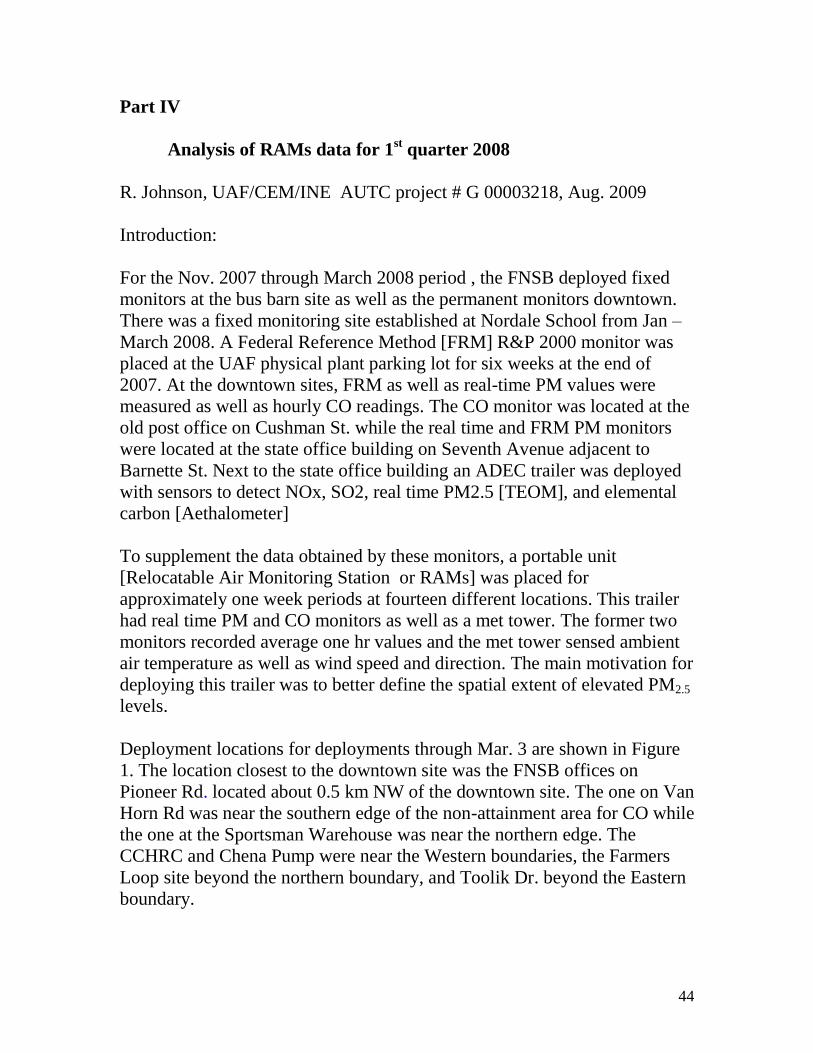
44
Part IV
Analysis of RAMs data for 1st quarter 2008
R. Johnson, UAF/CEM/INE AUTC project # G 00003218, Aug. 2009
Introduction:
For the Nov. 2007 through March 2008 period , the FNSB deployed fixed
monitors at the bus barn site as well as the permanent monitors downtown.
There was a fixed monitoring site established at Nordale School from Jan –
March 2008. A Federal Reference Method [FRM] R&P 2000 monitor was
placed at the UAF physical plant parking lot for six weeks at the end of
2007. At the downtown sites, FRM as well as real-time PM values were
measured as well as hourly CO readings. The CO monitor was located at the
old post office on Cushman St. while the real time and FRM PM monitors
were located at the state office building on Seventh Avenue adjacent to
Barnette St. Next to the state office building an ADEC trailer was deployed
with sensors to detect NOx, SO2, real time PM2.5 [TEOM], and elemental
carbon [Aethalometer]
To supplement the data obtained by these monitors, a portable unit
[Relocatable Air Monitoring Station or RAMs] was placed for
approximately one week periods at fourteen different locations. This trailer
had real time PM and CO monitors as well as a met tower. The former two
monitors recorded average one hr values and the met tower sensed ambient
air temperature as well as wind speed and direction. The main motivation for
deploying this trailer was to better define the spatial extent of elevated PM2.5
levels.
Deployment locations for deployments through Mar. 3 are shown in Figure
1. The location closest to the downtown site was the FNSB offices on
Pioneer Rd. located about 0.5 km NW of the downtown site. The one on Van
Horn Rd was near the southern edge of the non-attainment area for CO while
the one at the Sportsman Warehouse was near the northern edge. The
CCHRC and Chena Pump were near the Western boundaries, the Farmers
Loop site beyond the northern boundary, and Toolik Dr. beyond the Eastern
boundary.

45
Results:
A summary of the RAMs data through Feb 29, 2008 appears in Table I.
These data were obtained starting with average hourly values over the
deployment periods indicated. Columns 1, 3, 5, and 8 define the locations of
the monitors as well as deployment dates while PM and CO data are
presented in columns 2 and 4 and 6 and 9 respectively. In columns 7 and 10
appear the ratios of CO to PM. Each PM2.5 or CO value in Table I represents
an average of multiple hourly averages. For example, the first two PM
entries for Jan 6-9 represent the average of about 96 values [4 days worth of
hourly averages]. Sometimes, one or a few hourly averages were missing
from the data set. The purple values in the rows labeled ratios represent the
rations between values at the RAMs sites to the downtown values. If one
looks at the ratio of RAMs PM2.5 to the downtown average PM2.5 during
the deployment periods, four sites [FNSB offices, Chena Pump, Toolik Dr.
and Sportsmans Warehouse] had ratios greater than 0.6. But, the Van Horn
site [ratio = 0.44] had the highest average PM value of all the RAMs sites
[32.1 g/m3]. The other sites had ratios were less than 0.2. We also looked
at the correlation coefficients between the PM2.5 levels at the RAMs’ sites
and downtown. We found that only the FNSB offices and Sportsman
Warehouse sites had positive r values plus R2 values greater than 0.50. The
Van Horn and Farmers Loop sites had positive [very week] correlations with
R2 values of 0.27 and 0.25 respectively. The other four sites experienced
either negative correlations or positive ones with R2 less than 0.16.
The 4 to 8 day average PM values downtown ranged from 14.5 to 73.4
g/m3 while the range at the RAMs sites varied from 4.3 to 32.1 g/m
3.
For CO, the same four sites as for PM2.5 had ratios of CO at the RAMs sites
to the corresponding downtown sites > 0.60. CO to PM2.5 ratios in columns
7 and 10 fell between 0.015 and 0.06. In other words, for the downtown site
as well as the eight represented RAMs sites, the PM2.5 values in g/m3 were
from 17 to 67 times greater than the CO values in ppm. The multi-day CO
average values ranged from 0.33 to 1.07 ppm.
Figs 2 – 13 represent characteristic plots of PM2.5 values for selected RAMs
sites together with corresponding values for the downtown site. The first
three are for the core downtown area, the next three for nearby locations just
north and south of the core area respectively, the next four for outlying sites
exclusive of N Pole and the last two for N Pole. We have not presented data

46
beyond March 3 as the average daily PM2.5 values during that period were
less than 8.5 except for one day at 15.3 g/m3 for the RAMs sites and less
than 15.5 except for one day at 27.6 g/m3 at the downtown site. The
average daily downtown PM2.5 for March was 10.5 g/m3. These are to be
compared with daily downtown values averaging 26.0 for January and 31.7
g/m3 for February.
Some figures such as 2 and 3 have individual hourly averages presented for
the dates indicated. With Fig. 2 covering the period from Jan 11 through Jan
17, there are close to 7 x 24 = 168 data points [the number is slightly less
because of some invalid data]. Other figures such as Fig. 4 show composite
hourly averages. Hence, no matter how many days are represented on such
figures, there are only 24 data points for each site. One would be the average
of all the PM2.5 values from 12 till 1 AM, the next the average from 1 till 2
AM, etc.
On some figures, the hourly PM averages for a RAMs sites are plotted
versus the corresponding values for the fixed downtown site. On others, each
of these two sets of values is plotted versus time. If the RAMs values are
much lower than the downtown values [cf. Figs 8 -10], they are multiplied
by a scaling factor to make comparison of the two levels more obvious. The
hourly downtown PM values exceeded 100 g/m3 at least once each day
during the Feb 3-10 cold snap and for 5 hrs during the mid afternoon and
evening on Jan 30.
R2 values either appear on the figures or next to the figures. If there is a
negative correlation, this is noted. Not shown are the downtown ambient
temperatures which averaged – 19 oC and -17
oC for January and February
respectively. The Jan T ranged from – 35 on Jan 14 to 1 oC on Jan 27. The
Feb T ranged from – 37 on Feb 7 to 8 oC on Feb 20 with T frequently less
than – 30 oC from Feb 3 – 9. During this period, a diurnal T variation of
about 6 oC was evident. But, the PM variation did not follow the same
pattern. The average wind speed at the various RAMs sites from Feb 1
through Mar 3 was 2.6 mph with values exceeding 10 mph midday on Feb
15 and from 11 AM until past midnight on Feb 29. During these periods, the
PM values were less than 7 g/m3 with 10 of 12 hourly averages equal to 0
between 6 AM and 5 PM on Feb 29.

47
Figs 14-18 incorporate selected CO data either versus time or versus PM at
four RAMs locations. The last figure shows both CO and PM vs. time with
the CO values multiplied by 30 to allow for easier comparison with the
corresponding PM values. We have omitted several data points with
questionably high CO values. Fig 19 illustrates the importance of wind
speed on PM levels.
Discussion of results:
It is clear from looking at Figs. 2-4 that the particulate levels at the FNSB
offices on Pioneer Rd. are highly correlated with those at the downtown PM
site. Earlier we found this to be the case between the FNSB bus barn and the
downtown site. Whether one looks at all the hourly values [Fig. 2 and 3], the
composite hourly values [Fig. 4], or the average daily values [not shown],
the R2 values are greater than 0.83 with a positive correlation. This implies
that over 83 % of the variations at the office location are associated with
variations at the downtown post office. This strong correlation is expected
since these sites are about 0.5 km apart with heavily trafficked roads nearby.
The highest composite average hourly values occurred between 11 AM and
7 PM at both sites. The highest individual hourly value of 62.1 g/m3
occurred at the offices at noon on Jan 14. At this same time the value
downtown was 80.7 g/m3 which was the third highest hourly value at this
location during this time period. The lowest values at each location of less
than 2 occurred during the early morning hours. The lowest average daily
temperature occurred on Jan 14 with values less than – 40 downtown from 8
AM until noon.
Data for the Sportsman’s Warehouse site appears in Figs 5 and 6 indicates
the correlation with downtown is fair with R2 = 0.53 using the multi-day
composite hourly averages. One can see that the composite hourly values
rise as morning traffic picks up and the downtown nighttime values rise
from the evening rush hour until 11 PM while those at the Warehouse flatten
out during the evening. Fig 5 includes data from Feb 21 while Fig 6 does not
since seven hourly RAMs values from Feb 21 were invalid which would
have affected the composite hourly averages. The Warehouse is located 2.3
km from downtown and has two major roads [Johansen Expressway and
Steese Highway] located nearby.

48
The Van Horn site [Fig 7] revealed a weak correlation with downtown with
an average PM value of 32.1 during the Feb 8-13 time frame. This site is
about 2.7 km SE of downtown with a modest amount of traffic including
some truck traffic.
The three RAMs sites [cf Figs 8 -10] that had average PM to downtown PM
ratios less than or equal to 0.20 were all located from about 5.6 to 8.2 km
from the downtown site and not near heavily trafficked roads. They all had
R2 values less than 0.30 with one [CCHRC] exhibiting an inverse
correlation. [distances from downtown in km; CCHRC = 5.6, Bonner St =
5.9., Red Fox = 8.2].
The Chena Pump Rd site [Fig 11], located 8.8 km W of downtown, mostly
had lower PM levels than downtown with very little correlation between the
two sites. Since this site was at a small business location, it likely had more
entering and leaving traffic during the day than a residence would have.
Thus may explain why a couple of the composite hourly values exceeded
those downtown.
Toolik Rd in N Pole is 13.5 km SE of downtown. With the data appearing
on Fig. 12, this site revealed the strongest negative correlation with the
downtown data. The downtown values rose during morning rush hour and
stayed elevated through the evening rush hour. The N Pole data rose from
about 4 PM till about 1 AM, fell till about 10 AM, rose from 11 AM till 1
PM and then fell till 3-4 PM. We already found a high correlation between
the downtown values and local traffic. The traffic volume near the N Pole
site was much lower than downtown but still likely experienced a morning
peak around 8-9 AM.. But, the home at which the RAMs was deployed as
well as four neighboring homes had wood stoves. The fact that the N Pole
data rose from late afternoon till around 1 AM is consistent with firing
patterns for wood stoves.
If we take a more detailed look at the N pole data [Fig. 13] considering the
individual [as opposed to composite] hourly averages, we find the N Pole
PM is higher than that downtown during the wee morning hours Sat, Sun,
and Monday. This is consistent with wood stove firing patterns. During the
first 3 of these 6 days, the ambient temperature was less than – 29 oC so
there would be ample motivation to use wood stoves.

49
Analysis of the data on Figs 14 -18 reveals moderate correlations between
CO and PM which is expected for those sites where motor vehicles are
important contributors to PM. One would expect this to be the case for the
FNSB offices, Sportsmans Warehouse [in a large shopping complex] and
Van Horn Road [truck traffic]. The good correlation for Van Horn Road may
be partially associated with the truck traffic as older heavy duty trucks can
be significant CO and PM emitters. At first glance, seeing a good correlation
for Toolik Dr in N Pole [Fig. 15] is surprising. But, if the PM is coming
from older wood stoves, having significant CO emissions also can be
possible. From the data shown on Fig 19, one can see that PM2.5 levels are
strongly influenced by wind speed. At moderate wind speeds during the
early morning hours of Feb 29, the PM levels are low at Sportsman’s
Warehouse partially because the traffic flows are low. But, as the traffic
picks up during the day, the PM levels are essentially zero due to strong
winds. As the speed falls in the evening, the PM levels rise a little but are
still low since the wind speed is still more than 10 mph.
The fact that three out of the four RAMs sites that had PM to downtown PM
ratios greater than 0.60, also had CO ratios greater than 0.60 indicates that
the CO cloud may extend over a similar area as the PM cloud. But, more
data is needed to confirm this.
Using the BAM data, for the downtown site, the daily PM2.5 35 g/m3
averages were exceeded 6 times in Jan and 7 times in Feb. For the RAMs
sites, exceedances occurred twice each month [coincident with downtown
exceedances]. So, extending our data collection network didn’t extend the
number of possible violations with respect to 24-hr PM levels.
Tables and Figures for 2008 RAMs Analysis

50
Figure 1 Fairbanks Map with RAMs and other key Locations
Distances from downtown site in km: FNSB offices- 0.5 Sportsmans Warehouse - 2.3
Van Horn - 2.7 bus barn - 3.5 CCHRC - 5.6 Bonner St [near F Loop] - 5.9
Red Fox Dr. - 8.2 Chena Pump 8.8 Toolik Dr. – 13.5

51
2008 PM 2.5 2008 CO Ratios bet 2008 CO Ratios bet
Jan 6-9 Feb 1-6 Jan 6-9 CO and PM Feb 1-6 CO and PM
Downtown 24.15 50.63 Downtown 0.78 0.032
CCHRC 4.32 Red F Dr 9.94 CCHRC 0.26 0.060 Red F Dr missing
Ratio 0.18 0.20 Ratio 0.33 data
R^2 [avg hrly vls] 0.30 0.03
neg slope
Jan 11-17 Feb 8-13 Jan 11-17 Feb 8-13
Downtown 27.50 73.36 Downtown 0.85 0.031 1.07 0.015
FNSB offices 19.04 V Horn Rd 32.10 FNSB offices 0.76 0.040 V Horn Rd 0.88 0.027
Ratio 0.69 0.44 Ratio 0.89 0.82
R^2 [avg hrly vls] 0.84 0.27
Bus Brn 24.90 0.87
Jan 18-23 Feb 15-19 Jan 19-23 Feb 15-19
Downtown 28.00 23.01 Downtown 0.87 0.031 0.89 0.039
near F Loop 7.20 C Pump 15.67 near F Loop 0.43 0.060 C Pump 0.8 0.051
Ratio 0.26 0.68 Ratio 0.49 0.90
R^2 [avg hrly vls] 0.25 0.16
Jan 25-30 Feb 22-29 Jan 25-30 Feb 22-29
Downtown 45.10 14.77 Downtown 1.02 0.023 0.88 0.060
Toolik Dr-N.P. 28.88 Sportsman Warehse9.84 Toolik Dr-N.P. 0.5 0.017 Sportsman Warehse0.54 0.055
Ratio 0.64 0.67 Ratio 0.49 0.61
R^2 [avg hrly vls] 0.51 0.53
neg slope
Table 1 Summary of RAMs data from Jan 1 through Feb 29 2008
PM 2.5 FNSB Jan 11-17 2008
R2 = 0.8313
0
10
20
30
40
50
60
70
0 20 40 60 80 100
downtown avg hrly vls [ug/m^3]
FN
SB
off
ice
s
Figure 2 Jan 11-17 RAMs data with individual hrly vls

52
PM 2.5 hrly vls Jan 2008
0
10
20
30
40
50
60
70
80
90
0 50 100 150 200
Time from 0 AM Jan 11
ug
/m^
3
downtown
FNSB offices
Figure 3. Jan 11 – 17 RAMs data vs time
Avg hrly PM2.5 Jan 11 - 17
R2 = 0.8384
0
5
10
15
20
25
30
35
15 20 25 30 35 40
downtown 2008 composite hrly vls
FN
SB
off
ice
s
Figure 4 Jan 11-17 RAMs data composite hrly vls

53
FNSB PM 2.5 hrly vls Feb 21 -
Mar 3 2008
R2 = 0.4571
0
10
20
30
40
50
0 20 40 60 80
Downtown PM
Sp
tsm
an W
areh
se
Figure 5 Feb 21-Mar 3 RAMs data with individual hrly vls
R2 = 0.53
Figure 6 Feb 22 – Mar 3 RAMs PM data vs time for composite hrly averages
FNSB avg hrly PM 2.5 2008
0
10
20
30
0 10 20 30
hr of day Feb 22 - Mar 3
ug
/m^
3
downtown
Sportsmans
warehouse

54
R2 = 0.27
Figure 7 Feb 7 – 13 RAMs PM data vs time for composite hrly averages
R2 = 0.025
Figure 8 Feb 1 – 6 RAMs PM data vs time for composite hrly averages
FNSB PM 2.5 composite hrly vls Feb 2008
0
10
20
30
40
50
60
70
0 10 20 30
time of day Feb 7 - 13
ug
/m^
3
downtown
V Horn Rd
FNSB PM 2.5 Feb 1-6 2008
[composite hrly averages]
0
20
40
60
80
100
0 10 20 30
time of day
ug
/m^
3
downtown
4 x red fox

55
R2 = 0.30
[negative correlation]
Figure 9 Jan 6 – 9 RAMs PM data vs time for composite hrly averages
R2 = 0.25
Figure 10 Jan 18 - 23 RAMs PM data vs time for composite hrly averages
FNSB PM2.5 Jan 6-9 2008
0
10
20
30
40
50
60
70
80
0 10 20 30
hr of day
CC
HR
C
downtown
6x CCHRC
FNSB PM 2.5 Composite hrly
averages
0
10
20
30
40
50
60
0 10 20 30
hr of day Jan 18-23 2008
ug
/m^
3
downtown
3x vls near F
Loop

56
R2 = 0.16
Figure 11 Feb 14 – 21 RAMs PM data vs time for composite hrly averages
R2 = 0.51
[negative
correlation]
Figure 12 Jan 25 - 30 RAMs PM data vs time for composite hrly averages
FNSB PM 2.5 2008
0
10
20
30
40
50
60
0 10 20 30
hr of day Jan 25-30
ug
/m^
3
downtown
Toolik Dr
FNSB composite avg hrly PM2.5 2008
0
5
10
15
20
25
30
0 10 20 30
hr of day Feb 14 - 21
ug
/m^
3
downtown
Chena Pump

57
FNSB PM 2.5 hrly vls 2008
0
20
40
60
80
100
120
140
160
180
0 50 100 150
hrs from 0 AM Jan 25
ug
/m3
downtown
Toolik Dr.
Figure 13 Jan 25 - 30 RAMs hourly PM vs time Jan 25 is Fri [< -30 Jan 25 8 PM till 2 PM 27th
]
AAQ at FNSB office bldg 2008 wo
CO outlier
R2 = 0.4849
0
0.5
1
1.5
2
2.5
3
3.5
4
0 20 40 60 80
PM 2.5 for Jan 11 - Jan 17
CO
[p
pm
]
Fig. 14 Jan 11- 17 CO vs PM

58
AAQ at Toolik Dr. N. Pole 2008
R2 = 0.7841
0
0.2
0.4
0.6
0.8
1
1.2
1.4
1.6
0 20 40 60 80 100
PM 2.5 from Jan 25 till 11 AM Jan 28
CO
[p
pm
]
Fig. 15 CO vs PM for Jan 25 – Jan 28
AAQ at Sportsmans Warehouse 2008
R2 = 0.3728
0
0.5
1
1.5
2
2.5
3
3.5
4
4.5
5
0 10 20 30 40 50
Hrly PM 2.5 Feb 21 - Mar 3
CO
[p
pm
]
Fig 16 CO vs PM for Feb 21 – Mar 3 2008

59
AAQ at FNSB Van Horn Rd 2008
R2 = 0.7252
0
0.5
1
1.5
2
2.5
3
0 50 100 150
PM 2.5 Feb 7 - 14
CO
[p
pm
]
Fig. 17 CO vs PM for Feb 7 -14 2008
AAQ V Horn Rd 2008
0.00
20.00
40.00
60.00
80.00
100.00
120.00
140.00
0 50 100 150 200
Hrs past 0 AM Feb 7
ug
/m^
3 o
r p
pm
PM 2.5
30*CO
Fig 18 AAQ from Feb 7 – Feb 14 20008

60
Notes: PM peaks at 21, 44, 60, 85 at 9 PM, 8 PM, noon and 1 PM with T = - 35, -32, -34,
and -34 o C respectively. Then T warmed to > - 25 C. Feb 7 is a Thur so peaks occurred
midday on Sat and Sun.
Sportsman's Warehouse 2008
0
2
4
6
8
10
12
14
16
18
0 5 10 15 20 25 30
Time on Feb 29 2008
win
d s
pe
ed
or
PM
WS [mph]
PM 2.5
Fig 19 Influence of wind speed on PM for Feb 29, 2008

61
Part V
Transportation System Management and Travel Demand Management
Strategies for Vehicle Traffic and PM 2.5 Reduction
Ming Lee
Introduction
There are a variety of Transportation System Management (TSM) strategies being
applied in many metropolitan areas throughout the United States for the purpose of
improving traffic flow on existing roadway systems. TSM typically deals with the supply
side of a transportation system such as the coordination of traffic signals along a corridor
to relieve congestion. To achieve maximum benefits of congestion relief, TSM strategies
often work in conjunction with Transportation Demand Management (TDM), with the
intention of reducing the demand for travel to enhance the effectiveness of system
management.
It is noted that for the reduction of vehicle traffic and emissions in the Fairbanks North
Star Borough (FNSB), the most effective measures are those that reduce the amount of
traffic on the roadway system, because there is very little traffic congestion in the area.
The effectiveness of traffic flow improvement in emission reduction is limited when
traffic on most of the major roadways can flow freely. For this study, we examine the
potential effectiveness of TSM/TDM control strategies in vehicle traffic reduction. The
control strategies examined here are those that have been applied elsewhere in the US
with positive results. The newly developed Travel Demand Forecasting (TDF) model for
the Fairbanks Metropolitan Area Transportation System (FMATS) is applied to assess the
effectiveness of these strategies in vehicle trip reduction. FMATS is the designated
Metropolitan Planning Organization (MPO) for the FNSB and the cities of Fairbanks and
North Pole.
Overview of the FMATS Travel Demand Forecasting Model
A TDF model typically divides the modeling area into Traffic Analysis Zones (TAZ), and
each TAZ has household and employment data identified for the purpose of trip
generation. This household and employment data are used by the model to predict trip
productions and attractions (trip ends) for each individual zone. For modeling purposes,
the TAZs are connected by a computerized planning network that is defined by links and
nodes, representing the actual roads and intersections in the area. Each roadway link is
defined by specific data that generally include roadway length, travel speed, number of
lanes, roadway capacity.

62
The updated FMATS TDF model continues to use modified version of the traditional
four-step modeling process. In more general terms these steps are as follows:
1. Trip Generation – This step predicts the number of person trip that are generated
by and attracted to each defined zone in a study area. This results in trip
Productions and Attractions for each zone by trip purposes. The FMATS TDF
model divides all trips into 3 trip purposes:
Home-Based Work (HBW)
Home-Based Non-work (HBNW)
Non Home-Based (NHB)
2. Trip Distribution – This step connects trip ends estimated in the Trip Generation
process to determine number of person trip interchanges between each zonal pair.
This results in Production-Attraction (P-A) tables that quantifies the number of
persons that will travel between one zone and all other zones for different trip
purposes.
3. Mode Choice – This step allows the model to consider different travel modes
(vehicles, transit, bicycle, pedestrian, etc) used for each zonal interchange. For
many large urban areas, transit is an important factor; however for Fairbanks,
transit and other modes make up a very small percentage (see the percentage of
people who take bus to work in Figure 2) of the total daily trips. The FMATS
model only considers vehicle trips, and the mode choice step is skipped.
4. Trip Assignment – This step assigns zone-to-zone vehicle trips to specific travel
routes, generally based on factors such as the fastest total travel time. For a
model without a mode choice component, the person trips in the P-A table are
first converted to vehicle trips by vehicle occupancy calculation. Purpose-specific
vehicle occupancy rates (i.e., average number of persons per vehicle) are applied
to the P-A table to convert person trips to vehicle trips for particular trip purposes.
Before assignment, all the 24 hour vehicle trips will then be distributed to
different time periods (e.g., AM peak, PM peak, and off-peak) during the day.
After assignment, the sum of all trips for each link during a particular time period
is then calculated as the estimated traffic volume on that link. The model is able
to adjust travel speeds and add delays on roadway facilities that are more heavily
used. If necessary, the model reassigns trips to less congested travel routes, in an
effort to simulate every day travel choices that drivers make in the real world.
In 2008 the FMATS TDF model was updated with the most recent employment data and
calibrated with the latest traffic counts. This version of the TDF model was used to
produce estimates of system-wide Vehicle Miles Traveled (VMT) for both the 2008
baseline and 2035 Long Range Transportation Plan scenarios. The VMT estimates were
used in the latest CO conformity analysis for the FMATS planning area.

63
Figure 1 shows the TAZs of FMATS MPO boundary. The CO non-attainment area is
enclosed by the dash line in Figure 1. The area represents the urbanized areas of
Fairbanks and North Pole. It is noted that the newly designated PM 2.5 non-attainment
area for the FNSB is actually larger than the MPO boundary. Currently, the FMATS
TDF model does not cover the entire PM 2.5 non-attainment area. In analyzing the
potential trip reduction of TSM/TDM strategies, we choose to track the VMT and total
traffic in the CO non-attainment area because it gives us an indication of how much
traffic reduction and subsequently PM 2.5 reduction can occur in the urbanized areas of
FMATS when various TSM/TDM strategies are applied.
Figure 1 FMATS MPO and CO Non-Attainment Area Boundary
Evaluation of Vehicle Trip Reduction Strategies in Vehicle Trip Reduction
We examined many TSM/TDM measures implemented in metropolitan areas in the US.
Although road pricing as a TSM strategy has been implemented in the U.K and other
countries in the world for purposes of vehicle trip reduction in heavily congested areas, it
has not been applied in the US. While assembling the list of potential strategies for
consideration, we also take into account the possibilities for the measures to be
implemented in the FNSB. For example, biking and walking are not viable transportation
options for most people in FNSB during December and January when the average
temperature is often below zero. In addition, measures that target improvement of
signalized intersections and traffic flow movement will not have much effect in the
FNSB, because there is very little congestion in Fairbanks.

64
After examining the potentials for applications in FNSB, we choose to evaluate three
major strategies that have been proven effective for traffic reduction: work from home
with flexible work hours, increase car pool percentage, and increase bus ridership.
Strategy 1: Flexible Work Schedule and Work at Home Programs
Many metropolitan areas have employer-sponsored programs aimed at reducing weekday
commuter trips. For example, Washington State requires employers with more than 100
full-time employees who arrive to work between 6 and 9 a.m. in a county of more than
150,000 population to sponsor flexible work schedule programs. Some of such programs
allow the employees to have a compressed work week. For example, employees can
choose to have four 10-hour days per week rather than five eight-hour days. Others allow
employees to work on a custom schedule that accommodates unique personal needs or a
carpool or vanpool schedule. Many employers have also started work at home (a.k.a.,
telecommute) programs for the employees.
To model trip reduction attainable with flexible work schedule and work at home
programs, we reduce the home-based work (HBW) production-attraction table produced
after the trip distribution step of the TDF model. The HBW production-attraction table
contains the number of persons who will travel for work between the origin and
destination zones. Reducing numbers of the table represents the number of persons
participating in the programs to stay at home for a particular weekday. We then run the
TDF model with the reduced HBW production-attraction table to estimate how much and
where the reduction in traffic will occurs.
According to data from the American Community Survey released by the US Census
Bureau in 2005, 39,164 workers commuted to jobs in Fairbanks North Star Borough,
Alaska, taking on average 17.3 minutes each way. The percent of commuters by means
of transportation is shown in Figure 1.

65
Figure 1 Percent of Workers by Means of Transportation to Work* * Source: 2005 American Community Survey
Table 1 applies the percentages of transportation means to work in Figure 1 to the total
number of commuters in FNSB. The results are the actual numbers of persons in each
transportation mode categories.
Table 1 Transportation Means to Work in FNSB
Means to work Percentage Number of persons Number of Commuters
work at home 2 800 (stay at home)
taxicab 3 1,199 1,199
walked 4 1,598 1,598
biked 1 400 400
public
transportation 1 400 400
Car pool 13 5,195 5,195
Drive alone 76 30,372 30,372
Total 100 39,964 39,164
We run the model by removing 1%, 2% and 5% of total commuters from the HBW
production-attraction table. The removed production and attraction represent the
commuters who stay at home on a particular work day via flexible work schedule
programs. The purpose of running the model with different reduction percentages is to
assess the elasticity of traffic reduction associated with increase in the participation of
work at home programs. Table 2 summarizes the results of the model runs. It is noted
that commuter trips account for approximately 20% of all trips (e.g., home-based non
work and non-home based) in the modeling area. Thus, a 5% reduction in commuter
trips results in just 1.2 % of system-wide VMT reduction.

66
Table 2 Summary of Work-at-Home VMT and Traffic Reduction
Scenarios
Total Daily
System-wide
VMT
(vehicle-mile)
Reduction
(%)*
Total daily VMT in
the CO non-
attainment
(urbanized) area
(vehicle-mile)
Reduction
(%)*
Total Daily
System-wide
traffic
(vehicles)
Reduction
(%)*
Total daily traffic
in the CO non-
attainment
(urbanized) area
(vehicles)
Reduction
(%)*
2008 Existing
condition 1,861,073
955,585
7,539,322
5,927,540
1% of existing
commuters
stay at home
1,856,646 0.24% 954,204 0.14% 7,519,925 0.26% 5,912,539 0.25%
2% of existing
commuters
stay at home
1,852,212 0.48% 951,802 0.40% 7,504,039 0.47% 5,900,545 0.46%
5% of existing
commuters
stay at home
1,837,518 1.27% 943,758 1.24% 7,447,416 1.22% 5,856,025 1.21%
* % Reduction is calculated as the difference in VMT between a scenario and the existing condition divided by the VMT of the existing condition

67
Strategy 2: Increasing Carpool
A carpool is another TDM program that is proven successful for commuter trip reduction.
A carpool is a group of two or more people who go to work or other destinations together
in a private vehicle. Carpool members usually work out agreements of who drives and
how often, and payments for gasoline and maintenance. During the period of high fuel
price in 2008, many workers who commuted to Anchorage organized carpools to save
fuel cost.
Currently, in FNSB there are 5,195 carpool commuters and 30,372 drive-alone
commuters. Assuming 2 persons for each carpool vehicle, the vehicle occupancy rate
(VOR) for commuter trips (i.e., HBW trips) in the FNSB is approximately 1.11. To
model the traffic reduction attainable with a carpool program, we run the model with
increased vehicle occupancy rates of 1.115, 1.118, and 1.149. The three VORs represent
approximately 1%, 2%, and 5% of total commuters who switch from driving alone to
two-person carpools. The results of the car pool model are shown in Table 3.

68
Table 3 Summary of Carpool Program VMT and Traffic Reduction
Scenarios
Total Daily
System-wide
VMT
(vehicle-mile)
Reduction
(%)*
Total daily VMT
in the CO non-
attainment
(urbanized) area
(vehicle-mile)
Reduction
(%)*
Total Daily
System-wide
traffic
(vehicles)
Reduction
(%)*
Total daily traffic
in the CO non-
attainment
(urbanized) area
(vehicles)
Reduction
(%)*
1.110 HBW
Vehicle
Occupancy Rate
(2008 Existing
condition)
1,861,073 955,585 7,539,322 5,927,540
1.118 HBW
Vehicle
Occupancy Rate
1,857,993 0.17% 954,905 0.07% 7,524,737 0.19% 5,916,200 0.19%
1.125 HBW
Vehicle
Occupancy Rate
1,855,079 0.32% 953,325 0.24% 7,513,984 0.34% 5,907,900 0.33%
1.149 HBW
Vehicle
Occupancy Rate
1,845,253 0.85% 948,084 0.78% 7,478,231 0.81% 5,880,897 0.79%
* % Reduction is calculated as the difference in VMT or traffic between a scenario and the existing condition divided by the VMT of the existing condition

69
Strategy 3: Increasing Bus Ridership
FNSB currently operates both fixed route buses and van services for the disabled. Given
the compact size of the Fairbanks urban area, the fixed route buses can be a convenient
means for many residents to commute to work. But, currently bus riders only constitute
approximately 1% of total commuters in FNSB.
With no information on FNSB’s plan of bus service operation in the future, we run the
model to estimate the amount of traffic reduction assuming that the existing bus services
will continue with the same route coverage and frequency, but incentives were created by
FNSB to encourage more drivers to ride buses to work.
By the methodology of TDF, the mode choice component is applied to the P-A table after
the trip distribution step. Because the FMATS TDF model does not have a mode choice
component, we use a simplified approach to estimate the traffic reduction attributed to
increased bus ridership. We apply reduction factors to the HBW P-A table to represent
the number of driving commuters who switch to riding buses for work. This part of the
modeling process is similar to the way we model stay at home traffic reduction.
However, because the bus routes are fixed, only commuters who live close to the bus
routes may switch from driving to taking buses for work. That is, only TAZs that are
within close proximity of the bus routes can be applied with P-A reduction factors.
We overlay bus routes on top of the model TAZ and identify the TAZs that are served by
the existing routes. We then multiply the P-A person trips between a pair of these TAZs
by reduction factors of 0.983, 0.966, and 0.915. The three reduction factors correspond
to approximately 1%, 2%, and 5% of total commuters who switch from driving to riding
bus. The results of the trip reduction modeling for the increased bus ridership are shown
in Table 4.

70
Table 4 Summary of Increased Bus Ridership Program VMT and Traffic Reduction
Scenarios
Total Daily
System-wide
VMT
(vehicle-mile)
Reduction
(%)*
Total daily VMT in
the CO non-
attainment
(urbanized) area
(vehicle-mile)
Reduction
(%)*
Total Daily
System-wide
traffic
(vehicles)
Reduction
(%)*
Total daily traffic
in the CO non-
attainment
(urbanized) area
(vehicles)
Reduction
(%)*
2008 Existing
condition 1,861,073 955,585 7,539,322 5,927,540
0.983 Trip
reduction due
to increased
bus ridership
1,857,635 0.18% 954,200 0.14% 7,520,560 0.25% 5,911,886 0.26%
0.966 Trip
reduction due
to increased
bus ridership
1,853,717 0.40% 951,391 0.44% 7,503,823 0.47% 5,897,701 0.50%
0.915 Trip
reduction due
to increased
bus ridership
1,847,016 0.76% 945,661 1.04% 7,471,302 0.90% 5,867,087 1.02%
* % Reduction is calculated as the difference in VMT or traffic between a scenario and the existing condition divided by the VMT of the existing condition

71
Comparison of the Effectiveness
All three TSM/TDM strategies/programs are evaluated with scenarios of 1%, 2%, and 5%
of the total commuters participating in each program. This setup enables the comparison
of effectiveness among the three programs. Comparing the numbers in Tables 2, 3, and
4, the work at home or flexible schedule is the most effective strategies in reducing
commuting VMT and traffic. The result is expected, because the reduction in the number
of commuters results in taking the vehicles of the stay-home workers completely off the
roads, while car pool programs retain a portion of the fleet on the road for carpools.
Although the increased bus ridership program also takes the vehicles of bus riders off the
road, the program is less effective than the work at home program, because only people
live close to the bus routes can take bus and bus routes run mostly around the urbanized
areas of Fairbanks. The work at home program is modeled with the assumption that
commuters within the entire MPO boundary can participate in the program. Thus, the
work at home program can have more VMT and total traffic reduction than the bus
program.
The bus program is in generally more effective than the carpool program, except for total
system-wide VMT. The reason is because that carpool program retains a portion of the
vehicles of the participating commuters, while the bus program takes these vehicles off
the road. The total system-wide VMT reduction for the carpool program is greater than
the bus program, because the bus program is restricted to the urbanized area while the
carpool program is not.
Potential PM 2.5 Reduction
One previously developed model shows that 30% of the PM 2.5 in the Fairbanks
downtown area may be due to vehicle traffic. Based on our analysis, we found that the
bus program is the most effective in reducing traffic in the urbanized area. Using the
reduction of traffic in the urbanized area of Fairbanks (CO non-attainment area) as the
traffic that contribute to the concentration of PM2.5 in downtown, for every 1% of
commuters (i.e., approximately 400 commuters) riding bus to work, we can expect a
0.079% (i.e., 30%* 0.26%) reduction in PM2.5 in the downtown area. The work-at-home
program can be the most effective for downtown PM2.5 reduction. If we can get 5% of
the total commuters (approximately 2000 commuters) to participate in the work at home
program, we can expect 0.36% (i.e., 30%* 1.21%) reduction in PM 2.5 concentration in
downtown Fairbanks.

72
Conclusions
Using the newly updated FMATS TDF model, we evaluate three TSM/TDM strategies,
work at home, increasing carpool, and increasing bus ridership for their effectiveness in
vehicle traffic and emissions reduction. All three TSM/TDM strategies/programs are
evaluated with scenarios of 1%, 2%, and 5% of the total commuters participating in each
program. The results show that the work at home or flexible schedule is the most
effective strategies in reducing commuting VMT and traffic, because the reduction in the
number of commuters results in taking the vehicles of the stay-home workers completely
off the roads
According to one model, 30% of PM2.5 concentration in downtown Fairbanks is caused
by vehicle traffic. Using the results of our evaluation, for every 1% of commuters (i.e.,
approximately 400 commuters) riding a bus to work, we can expect a 0.079% reduction
in PM2.5 in the downtown area. If 5% of the total commuters (approximately 2000
commuters) participate in the work at home program, we can expect 0.36% reduction in
PM 2.5 concentration in downtown Fairbanks. So, to achieve a significant reduction in
downtown PM2.5, we would need a major participation in programs such as these.

73
Part VI CMB Analysis; Cathy Cahill and Ron Johnson
There have been dozens of source apportionment studies for PM2.5 completed in the last
decade or so in the United States and elsewhere. The purpose of such a study is to
delineate the major sources that contribute to the observed concentrations of PM2.5 in the
atmosphere. Three widely used source apportionment techniques include positive matrix
factorization [PMF], UNMIX, and chemical mass balance [CMB]. Each of these
techniques attempts to explain the measured chemistry of the particles in the atmosphere
by looking at the chemical profiles for the sources. Others utilize meteorological data to
make inferences about sources. For example, if one had data on the temporal variation of
wind speed and direction, one could calculate the route taken by an air parcel prior to its
being sampled at a specific receptor and, by identifying specific sources that the air
parcel crossed, infer likely sources of the aerosols in the sampled parcel.
Studies conducted in the United States indicate that secondary sulfate originating from
coal-fired power plants and secondary organic matter originating from motor vehicle
emissions are major sources of observed aerosol. Separating the mobile sources into
gasoline and diesel categories has been a challenge due to mixture of vehicles on the
roads, the variability in mobile source emissions under different vehicle operating
conditions and the similarity of diesel exhaust to oil-fired home heating fuel emissions.
Other major source categories include biomass burning, crustal emissions from roads or
windblown dust, and specific industrial emissions such as identified smelters or
refineries. Interpretation of the source apportionment results requires human judgment.
Coutant et al, 2003, COMPILATION OF EXISTING STUDIES ON
SOURCE APPORTIONMENT FOR PM2.5, BATTELLE, prepared for
Emissions, Monitoring, and Analysis Division
Office of Air Quality Planning and Standards
U.S. ENVIRONMENTAL PROTECTION AGENCY
Research Triangle Park, North Carolina 27711
Receptor models use chemical and physical characteristics of particles or gases at both
sources and receptors as input variables. Chemical mass balance [CMB] models use
chemical compositions at receptors to estimate the contributions of different source types
to the observed quantities at the receptors. This is in contrast to dispersion models which
start with assumed source emission rates and then incorporate transport phenomena plus
chemical reaction mechanisms plus physical mechanisms such as sedimentation to
calculate concentrations at receptors. A CMB model estimates contributions from sources
of different types such as coal combustion rather than from individual emitters.
It is normally used to apportion PM that is directly emitted as opposed to secondary PM
formed by subsequent reactions in the atmosphere. An example of the former is soot
while nitrate compounds could be part of the latter. The model consists of a set of
equations relating chemical concentrations at the receptors to a linear sum of the source
concentrations times each source contribution fraction. A solution is typically found by

74
the method of least squares. A necessary condition for a solution to exist is the number of
species is at least equal to the number of sources. Appropriate statistical variables are
used to quantify parameters such as the source contribution estimate divided by the
standard error. The higher this value, the better. Another parameter is the ratio of the sum
of the source contributions to the measured mass at a receptor to the measured mass.
Acceptable values may range from 80 % to 120 % (Watson et al, 1990).
Watson, J., N. Robinson , J.C. Chow, R.C. Henry and B.M. Kim
T.G. Pace, E.L. Meyer and Q. Nguyen, The USEPAIDRI Chemical Mass Balance
Receptor Model, CMB 7.0., 1990, Environmental software, 5, no 1, pp 38 – 49
The model used in our study was CMB 8.2 developed by the US EPA. The source code,
executable code, and test cases are available from the EPA’s website
(www.epa.gov/scram001).
Results from Montana indicate the PM2.5 attributed to wood smoke via CMB 8.2 [range
from 56 to 82 %] was within 10 % of that inferred from 14
C data for five of six sites
{Ward, 2009). If the 14
C is present at atmospheric levels, it is assumed to be derived from
biomass burning. Meanwhile 14
C data collected at 4 sites in the Fairbanks NSB in Feb of
2009 indicate 43 % of the PM2.5 is from wood smoke.
We used SASS data obtained in downtown Fairbanks from 2005 – 2009, as well as in
North Pole, the FNSB bus barn, and various RAMs sites in 2009, for the PM2.5 chemical
concentration at the receptors. For the source profiles, we used profiles from numerous
studies including the Pacific Air Quality Study, the Northern Front Range Air Quality
Study, etc. obtained from the EPA CMB web site that incorporated profiles for dust, auto
emissions, biomass burning, coal power plants, secondary processes, as well as certain
industrial processes such as blast furnaces and kraft recovery boilers. These profiles
specify the fraction of each source’s aerosol that is due to a specific component and
highlight which components are specific to different sources. For example, zinc would
be an example of a species attributed to industrial processes using waste oil and soluble
potassium would be an example of a species that is attributed to wood smoke.
The results from the source apportionment conducted on the data from the downtown
Fairbanks site appear in Fig. 1 and reveal that biomass burning, auto emissions and dust
are all significant in the wintertime with biomass combustion contributing 78, 62, 51, and
53 % of the downtown PM2.5 for the months of November, December, January, and
February, respectively. The corresponding percentages for automobiles are 24, 17, 20 and
24 %. At the bus barn during January and February, 2009, [Fig. 2] biomass burning, auto
emissions and dust were each found to contribute about one-third of the PM2.5 mass.
Similar results were found for the North Pole site.
Ward, Tony, Univ. of Montana, July, 2009, presentation at Fairbanks Air Quality
Symposium.

75
Source Contributions to Total Particulate Load in Fairbanks
0
5
10
15
20
25
30
35
Jan Feb Mar Apr May Jun Jul Aug Sep Oct Nov DecMonth
PM
Co
nc
en
tra
tio
n (
ug
/m3
)
PCHC
AMNIT
AMSUL
FRNC
BOIL
BURN
AUTO
DUST
MARIN
Fig. 1 Source Contributions to Total Particulate Load in Fairbanks
Source Contributions to Total Particulate Load at the Transit Yard
0
5
10
15
20
25
30
35
Jan Feb MarchMonth
PM
Co
ncen
trati
on
(u
g/m
3)
PCHC
AMNIT
AMSUL
FRNC
BOIL
BURN
AUTO
DUST
MARIN
Fig. 2 Source Contributions to Total Particulate Load at the Transit Yard