HAL Id: hal-00522530https://hal-brgm.archives-ouvertes.fr/hal-00522530

Submitted on 30 Sep 2010

HAL is a multi-disciplinary open accessarchive for the deposit and dissemination of sci-entific research documents, whether they are pub-lished or not. The documents may come fromteaching and research institutions in France orabroad, or from public or private research centers.

L’archive ouverte pluridisciplinaire HAL, estdestinée au dépôt et à la diffusion de documentsscientifiques de niveau recherche, publiés ou non,émanant des établissements d’enseignement et derecherche français ou étrangers, des laboratoirespublics ou privés.

Development of a tool for managing groundwaterresources in semi-arid hard rock regions: application to

a rural watershed in South IndiaBenoît Dewandel, Jérôme Perrin, Mohamed-Salem Ahmed, Stéphanie Aulong,

Z. Hrkal, Patrick Lachassagne, M. Samad, S. Massuel

To cite this version:Benoît Dewandel, Jérôme Perrin, Mohamed-Salem Ahmed, Stéphanie Aulong, Z. Hrkal, et al.. De-velopment of a tool for managing groundwater resources in semi-arid hard rock regions: applicationto a rural watershed in South India. Hydrological Processes, Wiley, 2010, 24 (19), p. 2784-2797.<10.1002/hyp.7696>. <hal-00522530>

Development of a Tool for managing groundwater resources in semi-arid

hard rock regions. Application to a rural watershed in south India

B. Dewandel1,*, J. Perrin2, S. Ahmed3, S. Aulong1, Z. Hrkal4, P. Lachassagne1, M.

Samad5 and S. Massuel5

- 1- BRGM, Water Division, Resource Assessment, Discontinuous Aquifers Unit, Rue

Pinville 34 000 Montpellier, France; b.dewandel@brgm.fr; s.aulong@brgm.fr;

p.lachassagne@brgm.fr (* Corresponding author)

- 2- BRGM, Water Division, Resource Assessment, Discontinuous Aquifers Unit, Indo-

French Centre for Groundwater Research, Uppal Road, 500 007 Hyderabad, India. ;

perrin@ngri.res.in

- 3- National Geophysical Research Institute, Indo-French Centre for Groundwater

Research, Uppal Road, 500 007 Hyderabad, India, shakeelahmed@ngri.res.in

- 4- Charles University, Faculty of Science, Albertov 6, Prague 2, 128 43 Czech

Republic, Zbynek_Hrkal@vuv.cz

- 5- IWMI, International Water Management Institute, South Asia Sub-Regional Office,

ICRISAT, Patancheru, Hyderabad, India; m.samad@cgiar.org, s.massuel@cgiar.org,

a.mukherji@cgiar.org

ABSTRACT

Until recently, aquifers located in hard rock formations (granite, gneiss, schist) were

considered as a highly heterogeneous media, and no adequate methodology for groundwater

management was available. Recent research studies showed that when hard-rocks are exposed

to regional and deep weathering processes and when the geology is relatively homogenous, a

typical hard rock aquifer is made of two main superimposed hydrogeological layers each

characterized by quite homogeneous specific hydrodynamic properties: namely the saprolite

and the fissured layers. Therefore, for these cases, hard rock aquifers can be considered as a

multi-layered system.

Based on these works, an operational Decision Support Tool (DST-GW) designed for the

management of groundwater resources in hard rock area under variable agro-climatic

conditions has been developed. The tool focuses on the impact of changing cropping pattern,

1

artificial recharge and rainfall conditions on groundwater levels at the scale of small

watersheds (10 to about 100 km2 in case well-developed weathering profile). DST-GW is

based on the groundwater balance and the ‘Water Table Fluctuation Method’, well-adapted

methods in hard rock and semi-arid contexts.

Based on field data from an over-exploited south Indian watershed (58 km²), the model allows

calibrating, at watershed scale, the variation in specific yield of the aquifer with depth, as well

as the rainfall/aquifer recharge relationship. Seasonal basin-scale piezometric levels are

computed with an average deviation of ±0.56 m compared to measurements from 2001 to

2005. The model shows that if no measure is taken the water table depletion will induce the

drying up of most of the exploited borewells by the year 2012. Scenarios of mitigation

measures elaborated with the tool show that change in cropping patterns could rapidly reverse

the tendency and lead to a sustainable management of the resource.

This work presents the developed tool and particularly the hydraulic model involved in, and

its application to a case study. However, the purpose tool is applicable at watershed scale but

not design for the groundwater management of a very small area or for a single bore well.

Key words: groundwater management, hard rock aquifer, overexploitation, groundwater

budget, DST-GW

1. INTRODUCTION

Supplying 27 million hectares of farmland in India, groundwater now irrigates a larger area

than surface water (21 million hectares). This change has been extremely rapid since the start

of the ‘Green Revolution’ in the 1970s, when the number of borewells have shoot up from

less than one million in 1960 to more than 20 million presently. In consequence, and

especially in hard rock and (semi)arid areas that covers about 2/3 of the country, the

groundwater resource is highly stressed due to large abstraction of water by pumping for

irrigation. As a result, this overexploitation of the resource threatens the sustainability of

water availability and agricultural development. Therefore in these areas, it is necessary to

adapt the groundwater resource exploitation to its availability.

2

Until recently, aquifers located in hard rock formations (granite, gneiss, schist) were

considered as highly heterogeneous media, and adequate methodologies for groundwater

management were not existent. Recent studies conducted in African, European and Indian

basements (e.g., Omorinbola, 1982, 1983; Wright, 1992; Chilton and Foster, 1995; Owoade,

1995; Wyns et al., 1999; Taylor and Howard, 2000; Maréchal et al., 2004; Dewandel et al.,

2006; Krásný and Sharp, 2007; Maréchal et al., 2007, Courtois et al., 2008, Courtois et al., in

press, etc.) showed that when hard rocks are exposed to regional and deep weathering

processes and when the geology can be considered as homogenous, the aquifer is constituted

of two main sub-parallel hydrogeological layers, namely the saprolite, a clayey-sandy

material, and the fissured layers, generally characterized by a dense horizontal fissuring in the

first few meters and a depth-decreasing density of fissures. Usually, the total thickness of the

weathering profile is comprised between 50 to 100 m. Each layer can be considered as

homogeneous and is therefore characterized by quite homogeneous hydrodynamic properties

(Maréchal et al., 2004, 2007; Dewandel et al., 2006). For example in hard rock areas of India

and Africa, this homogeneity in term of layers thicknesses and hydrodynamic properties is

shown from 100 m to kilometric scale (e.g., Dewandel et al., 2006; Courtois et al., 2008,

Courtois et al., in press). Consequently, hard rock aquifers exposed to regional deep-

weathering processes can be considered as a composite aquifer constituted of two main layers

characterized by their own hydrogeological properties.

Based on this conceptual model of hard rock aquifers, the Indo-French Centre for

Groundwater Research (IFCGR- Hyderabad) has developed a Decision Support Tool for

sustainable groundwater management in semi-arid hard rock regions at watershed scale (DST-

GW). The main objective of the tool is to help stakeholders to visualise what would happen to

groundwater levels under different conditions of groundwater exploitation (irrigation),

implementation of artificial recharge structures, and rainfall scenarios. The hydraulic model

involved in DST-GW is based on the water table fluctuation method and groundwater budgets

performed at catchment scale (Maréchal et al., 2006). DST-GW predicts mean groundwater

levels at seasonal and watershed scale and is thus a lumped model. However, the purpose tool

is applicable at watershed scale, so it cannot be used for the groundwater management of a

very small area or a single exploited borewell.

For its scientific development, DST-GW has been implemented in a representative south

Indian watershed (Maheshwaram watershed; 58 km² in area, Fig.1) characterised by a granitic

3

basement, a relatively flat area (from 590 to 670 masl), semi-arid climatic conditions (mean

annual precipitation: 750 mm; potential annual evapotranspiration: 1800 mm; aridity index=

0.42), rural context, and groundwater overexploitation due to large amount of water pumped

for the irrigation of rice (210 ha during the dry season and 500 ha during the rainy season),

vegetables (15 ha), flowers (20 ha), fruit trees (47 ha) and grape (55 ha). The mean annual

groundwater abstraction at catchment scale is about 10 Mm3 (174 mm).

This work presents the developed tool and particularly the hydraulic model involved in, and

its application to the Maheshwaram watershed.

2. BRIEF DESCRIPTION OF THE TOOL

Figure 2 presents the break down structure of the tool.

DST-GW is composed of the following main active windows:

- Input data for groundwater budget computation: groundwater fluxes at basin scale (RF, Qin,

Qoff, PG, E, watershed scale piezometric levels; see Eqs.1 and 2), mean elevation, and mean

elevation of the bottom of the saprolite layer and of the bedrock (fresh basement). Input data

are averages at watershed scale,

- Calibration and validation of the hydraulic model, from previous data relationships at

watershed scale between elevation and specific yield as well as rainfall and recharge are

established. These relationships are used to compute theoretical water levels that are

compared to the ones observed. These relationships are used for computing future scenarios.

- Scenario: it comprises a modulus for creating the “most probable scenario” (i.e., the one that

predicts what should happen in the studied area according to agricultural, industrial, tourism

policies) and other scenarios for testing other strategies. For all the scenarios, groundwater

uses can be modified as well as rainfall conditions. This window also comprises input

information on exploited borewells (i.e., elevation of the base of the fissured layer), structures

favouring artificial recharge and rainfall historical data.

DST-GW is devoted to groundwater management in semi-arid hard rock areas. Scenarios

including impacts of rainfall change and/or changing cropping patterns can be tested and

groundwater levels forecasted. DST-GW is particularly well designed for watershed size

ranging from 10 to 100 km2 where geology, layers thicknesses of the weathering profile and

4

hydrodynamic properties can be considered as homogeneous. In addition and as a basic

prerequisite, the aquifer has to be unconfined to allow proper uses of groundwater budget and

water table fluctuation methods (see next section).

As a main result, the tool estimates mean groundwater levels at basin scale on a seasonal

time-step (for dry and rainy seasons only; two values per year) and an estimate of the drying

up of exploited borewells. Therefore, the tool is particularly well-suited for encouraging

discussions between stakeholders to favour the implementation of groundwater exploitations

strategies and regulations.

3. DESCRIPTION OF THE HYDRAULIC MODEL INVOLVED IN DST-

GW

The hydraulic component of DST-GW is based on the combination of the well-known ‘Water

Table Fluctuation (WTF)’ method and groundwater budget computation for estimating

aquifer specific yield and annual recharge (Maréchal et al., 2003 and 2006; Saha and

Agarwal, 2006.). This combination offers two main advantages while dealing with hard rock

aquifers and semi-arid context: i) no use of hydrodynamic parameters in the model except for

estimating some groundwater budget components, and ii) evapotranspiration from crops,

which can be the source of large uncertainties particularly in semi-arid climate, does not need

to be estimated as DST-GW focuses on groundwater fluxes only (recharge is computed with

WTF method). The only basic requirements to use this method are that the aquifer should be

unconfined and that dry and rainy seasons should be well differentiated (significant water

table rises and declines).

3.1 Groundwater budget equations

The basic equation governing the fluxes at the basin-scale into an unconfined aquifer is

(Schicht and Walton 1961):

SQQPGEQRFR bfoffin Δ++++=++ (1)

where R is the total groundwater recharge [mm], RF irrigation return flow [mm], Qin and Qoff

groundwater flow in and off the aquifer boundary [mm], E evaporation from water table

[mm], PG groundwater abstraction by pumping [mm], Qbf base flow (ground water discharge

to streams or springs; in mm), and ΔS change in groundwater storage [mm]. Due to the

5

relatively deep water table in the Maheshwaram watershed (more than 17 m), there are neither

springs nor contribution of groundwater to streams, consequently the base flow is nil (Qbf=0).

The methodology used to determine the unknown groundwater storage is the Water Table

Fluctuations method, which links the change in groundwater storage, ΔS, with resulting water

table fluctuations, Δh:

hSS y Δ=Δ . (2)

where Sy is the specific yield (dimensionless), or the effective porosity of the unconfined

aquifer.

Due to seasonal monsoon rainfall, piezometric levels display sharp rises and declines (see

Table 1). Therefore, the hydrological year can be divided into two distinct seasons: dry (Rabi,

November to May) and rainy (Khariff, June to October). Thus, combining the use of both

groundwater budget and water table fluctuation methods twice a year allows on the one hand,

the computation of the unknown parameter Sy during the dry season by assuming a nil

recharge in Eq.1, and on the other hand the computation of recharge during the rainy season

(i.e., with known Sy in Eq.1).

3.2 Estimation of the flow components

Application of the WTF method requires an accurate knowledge of all the components of the

budget, except recharge and specific yield, which are considered in this approach as unknown

parameters and are calculated using the combined method described above.

WTF method has been successfully applied to Maheshwaram watershed. Tables 1 and 2

summarize the seasonal and annual groundwater budget for the five studied hydrological

years (2001 to 2005). The next section briefly describes how the different components have

been evaluated. However, the reader may find additional information in Maréchal et al.

(2006) for all components of Eq.1 and the impact of their uncertainties on the groundwater

balance, Sy and R estimates, in Zaidi et al. (2007) particularly for h and Δh estimates

according to various observation networks and impact on balance, Sy and R, and finally in

Dewandel et al. (2008) for RF and PG estimates. Using such methods Maréchal et al. (2006)

showed that the maximum expected uncertainty introduced by the fluxes components of Eq.1

on the total groundwater recharge and the annual groundwater balance is about 20%.

6

Precise seasonal water level fluctuations (Δh) were obtained by establishing detailed

piezometric maps at the end of the dry seasons (in June) and at the end of the rainy seasons

(October-November) based on up to 165 piezometers (IFCGR and non-exploited borewells;

Fig.1). No measurements were perfomed in pumped wells and the rare cases of observed

drawdown in the monitored wells (monitoring of IFCGR observation wells; time recording

time interval: 15’) are never more than 10 to 20 cm, which is little compared to water table

fluctuations at seasonal scale (several meters). The relative error on the water table fluctuation

has been calculated by geostatistics and logically decreases with the number of measurements

(Tab.1). Mean seasonal piezometric levels were obtained from mapping and kriging of

piezometric data; Figure 3 presents one of the piezometric map and Table 1 the mean seasonal

piezometric levels at the catchment scale and the corresponding Δh with the relative error (±).

Groundwater abstraction (PG in Eq. 1) was evaluated by combining a well inventory database

(i.e., discharge rate of each exploited borewell) and daily duration of pumping, which have

been deduced from piezometric data influenced by exploited wells (Dewandel et al., 2008).

The mean annual groundwater abstraction (Mean annual in Table 2) is 174 mm, and has been

evaluated for all groundwater uses, i.e.: rice (86.8% of PG), vegetable (0.7%), flowers (0.8%),

fruit trees (2.5%), grapes cultivation (5.2%), domestic (1.7%) and poultries (2.3%). The

groundwater abstraction was found in accordance with the one evaluated from a land use map

using remote sensing technique (difference of about 5%, NRSA, 2003). Table 2 presents the

groundwater abstraction per season and per uses.

Irrigation return flows (RF in Eq. 1) were estimated for each irrigated crops, except for grapes

and fruit trees, which use drip irrigation technique; for these crops RF was assumed nil.

Irrigation return flows for rice, flowers and vegetables cultivation were estimated from a

hydraulic model that combines both unsaturated and saturated flow theory and few

information about the soil type, the meteorological conditions [rainfall and potential

evaporation], the frequency of irrigation and the cropping calendar (Dewandel et al., 2008).

The obtained irrigation return flow coefficients, i.e. the ratio of the irrigation return flow (RF)

to the abstracted flow (PG), are on average 47% for rice (PGrice/RFrice in Tab.2), 23% for

vegetables and 10% for flowers, and are similar to coefficients found in the literature

(APGWD, 1977; Chen et al., 2002; Jalota and Arora. 2002). As no information about return

flow from domestic and poultries uses was available, and since return flow may exist, a value

of 20% was assumed. On average, mean annual return flow from pumping corresponds to

7

about 72 mm meaning that about 42% of the groundwater abstraction returns back to the

aquifer.

Groundwater evaporation, E, was estimated using an empirical relationship established for

semi-arid environment that depends on groundwater level depth, z, (E=71.9z-1.49; Coudrain, et

al., 1998). In Maheshwaram watershed, it is a very small groundwater budget component, 2.3

mm/year, due to quite deep water levels (more than 17 m). Even if the proposed estimate is

probably not the best because of the use of an empirical relationship its order of magnitude is

outlined. In addition, because of its small amount compared to other fluxes this component

will not affect significantly the groundwater budget.

Horizontal in and out flows, Qin and Qoff, across the aquifer boundaries, were evaluated using

a finite-differences model run in steady state mode (Modflow; Maréchal et al., 2006). The top

of the fresh basement (Dewandel et al., 2006) and the piezometric map are used in

computation. The aquifer permeability has been assumed constant at the watershed scale and

equal to 4x10-6 m/s (Maréchal et al., 2004). Results show that Qin and Qoff are also small

components of the groundwater budget (annual balance: about -1 mm/year).

3.3 Computation of the specific yield and the recharge at the watershed

scale

3.3.1 Specific yield, Sy:

According to the different groundwater fluxes (see previous section), the specific yield, Sy, is

computed for each dry seasons at the watershed scale using Eqs. 1 and 2. As a consequence, a

set of couple of Sy versus range of piezometric fluctuations (Δh) is obtained, Δh being defined

by the average post- and pre-monsoon piezometric levels (see Table 1).

The bars in Fig. 4 illustrate the (Sy, Δh) couples for the dry seasons October 01-June 02 (Sy:

0.013), November 02-June 03 (Sy: 0.014), November 03-June 04 (Sy: 0.015) and November

04-June 05 (Sy: 0.014).

In the fissured zone of the weathering profile, aquifer permeability and storativity primarily

depends on the degree of weathering and thus on the density of fissures, which itself

decreases rapidly with depth (Acworth 1987; Wyns et al., 1999; Maréchal et al., 2004,

Dewandel et al., 2006). Moreover, it has been shown that fissure properties are characterized

by similar hydraulic properties whatever their location in the fissured layer (Dewandel et al.,

8

2006). Consequently, it is proposed to model the variation in Sy vs. elevation by the variation

in the percentage of fissures with the elevation. The percentage of fissures is deduced from a

statistical analysis based on flowmeter tests in borewells carried out in the study area (Fig. 5;

Dewandel et al., 2006). To compute the vertical variation in Sy at the watershed scale, the

fissured zone is discretized in five layers of equal thickness (layers L3 to L7; Figs. 4 & 5), and

the saprolite layer in two layers of equal thickness (layers L1 and L2).

First, the average specific yield of the investigated fissured zone, Sypond-FZ, is computed using

Eq. 3:

∑∑==

−ΔΔ=

n

ii

n

iiiyFZpondy hhSS

11/ (3)

where Syi are Sy estimates in the investigated intervals Δhi (see Table 1).

Then, assuming a linear relationship between Sypond-FZ and the percentage of fissures

encountered within the same investigated zone leads to estimate the average Sy per fissure,

Ratio%fiss.:

∑

∑

=

=

Γ

Γ= n

iii

n

iiFZpondy

fiss

X

SRatio

1

1_

.% (4)

where Xi is the percentage of fissure in the discretized layer i, Γi is the investigated fraction of

the discretized layer i.

Therefore, Eq. 4 is used for modelling the variation in Sy vs. elevation for the entire fissured

zone by multiplying the percentage of fissure of each layers by Ratio%fiss. For the saprolite

layer, weighted values of the investigated intervals within the saprolite layer are used. Figure

4 presents the modelled Sy at the watershed scale vs. elevation deduced from the four years of

records.

When all the data set (June 01 to June 05, 4 years) is used for calibrating the Sy model, it gives

for the fissured zone of the Maheshwaram granite aquifer an average Sy value of 8.0x10-3,

which is consistent with data obtain from pumping tests, in average 6.3x10-3 (Maréchal et al.,

9

2004), this validates the high elevation-decrease in Sy and shows the robustness of the

methods used for modelling Sy.

However, if required the Sy model can be changed and different Sy values can be prescribed to

each of the seven discretized layers. This option lets the users free to test any other hypothesis

concerning the variation in specific yield with elevation.

3.3.2 Recharge, R:

Once the Sy model is established, then the recharge model is computed using Eqs. 1 and 2, and

the groundwater budget components during the rainy seasons. This procedure is more

accurate than the classical water table fluctuation method which usually assumed a constant Sy

value for the entire aquifer thickness. It is why recharge values estimated in Maréchal et al.

(2006) are slightly different (Jun 02 - Nov 02: 70.5 against 70.8* mm; Jun 03 - Nov 03: 156.5

against 160.4* mm; * this study).

Based on the analysis of the complete data set (four years of records) and on the previously

defined Sy model, a linear relationship between recharge and annual rainfall is found (Fig. 6).

This model is thus applied to rainfall values for modelling the recharge at the watershed scale.

However even if the linear character of this relation is consistent with other studies carried out

in granitic areas of south India that use tritium as recharge tracer (Fig. 6; Rangarajan and

Athavale, 2000; Sukhija et al., 1996), the model computes higher values. Because of the use

of the WTF method, DST-GW computes an estimation of the total recharge at the basin-scale

while the tritium technique, a local approach, gives only the minimum recharge (‘direct’

recharge) and does not take account of both ‘indirect’ recharge, the percolation through rivers

and tanks beds, and ‘localized’ recharge through local geological or topographic variations

(Lerner et al., 1990; Maréchal et al., 2006). This is why values from DST-GW are higher. In

turn, this difference gives the maximum expected percolation at the watershed scale through

the tanks located in the study area that cover about 80 ha. The difference between the two

trends (positive value only) is used for estimating the maximum expected artificial recharge

from the tanks under variable rainfall conditions.

Once Sy and recharge models are calculated, the annual groundwater balance can be computed

for each hydrological year (Tab. 2).

For the Maheshwaram aquifer, the groundwater balance from 2001 to 2005 is very often

negative which illustrates the overexploited status of this aquifer. Only the year 2003 was a

10

‘positive’ year due to high and quite exceptional rainfall (1041 mm). On average (see Mean

annual in Tab. 2), annual depletion of groundwater levels is 1.5 m with a negative balance of

about -20 mm. This shows that even if rainy year may provide a significant increase of

groundwater levels, their frequency is too low to counterbalance the negative balance induced

by the pumping during ‘normal’ and ‘weak’ rainy years.

3.4 Computation of piezometric level and model sensitivity

3.4.1. Computation of piezometric levels

Piezometric levels computation either for validating the model or forecasting groundwater

levels under different abstraction and/or rainfall conditions, makes use of the Sy model, the

recharge model, and the variation in aquifer storage, ΔS which depends on the different

groundwater fluxes (see Eq. 1).

Computed piezometric level, ht+1, at time t+1 that corresponds to the next season can be

written as follows,

for ΔS ≥0:

⎥⎦

⎤⎢⎣

⎡−+−−Δ+= ∑

=+++

++

n

iiyiiiytit

iytt SYYShYSShh

1111

11 )()(1 (5a)

and for ΔS <0:

⎥⎦

⎤⎢⎣

⎡−+−−Δ+= ∑

=−+

−+

n

iiyiiiyitt

iytt SYYSYhSShh

111

11 )()(1 (5b)

where ht is the piezometric level at time t, ht+1, piezometric level at time t+1, Syi, specific

yield of the discretized layer i, ΔSt+1, storage variation at t+1,Yi= bottom of the discretized

layer i.

3.4.2. Sensitivity of the hydraulic model to the duration of the calibration period

Sensitivity of the hydraulic model has been evaluated through calibrations of Sy and recharge

models from different periods, i.e., from one year to four years of calibration (Fig. 7 a and b).

11

During these tests, Sy and recharge models are generated from the different prescribed

calibration periods (1, 2, 3 and 4 years), and sets of piezometric levels are computed with

these models for the entire available data set (June 2001 to June 2005; Fig. 7c). Finally, the

computed levels are compared to the ones observed and the piezometric observations beyond

the calibration period are used for validating the model. The deviation between observed and

computed water levels is expressed as follow:

∑ −=n

iisimiobs hhmDev ,,].[ (6)

where hobs,i and hsim,i are observed and computed piezometric levels respectively.

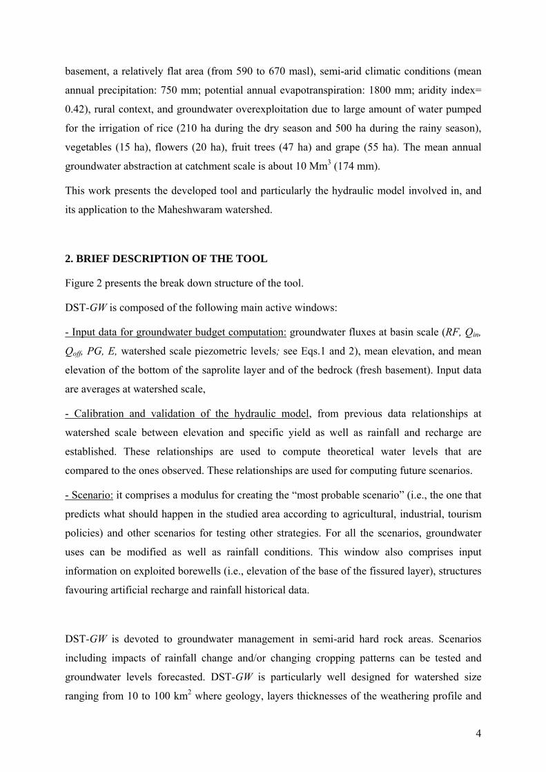
Figures 7 a and b show that with the analysed data set 3 years of calibration period are

necessary to obtain similar recharge and Sy models. Consequently, the difference between

observed and computed water levels is low for the models calibrated on 3 and 4 years of

records (Fig. 7c). One may thus assumed that continuing calibration beyond for 4 years, and

thus continuing to compute all groundwater fluxes components of Eq.1, should not drastically

change the these models. However, the calibration on 4 years is sensibly better (dev.=±0.56 m

against ±0.95 m for the 3 years calibration period; Fig. 7c) because during the fourth year of

record water levels were the deepest which has for consequence to improve the Sy estimate of

the deepest aquifer compartment, i.e. the fissured zone.

In the following sections, the hydraulic model established from the calibration on the entire

data set (4 years) is kept for further calculation. For this watershed, DST-GW models the

basin-scale piezometric levels with an average deviation of ±0.56 m from 2001 to 2005,

which shows the robustness of the model.

Once the hydraulic model is achieved, the user may proceed to the scenario creator modulus.

4. SCENARIOS

The scenario module, in addition to feed the model with additional data (borewell database,

historical rainfall data), is especially devoted to create a ‘reference scenario’ (i.e., business as

usual scenario) as well as additional scenarios. The ‘reference scenario’ or ‘most probable

scenario’ describes the future evolution of a site according to changes that are expected

through strategies planned at national or regional levels. The scenario module allows creating

theoretical scenarios in order to test the impact of different management measures upon the

12

groundwater resource. For every scenarios, the DST-GW’s user may i) change the abstraction

of the existing groundwater uses at seasonal time-step, or add new ones, ii) change future

annual rainfall, or /and iii) change the number or efficiency of artificial recharge structures.

As an example, two alternative scenarios are presented to help visualise and discuss their

impacts on the groundwater resource. However, these scenarios are theoretical and issued

from an optimisation approach that is not socio-economically sound since the development of

the socio-economic module (e.g., computation of farmer’s net returns) is not yet available.

4.1. Reference scenario

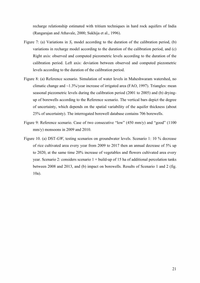
In this scenario, no climatic change is considered, and the rainfall scenario uses the past 20

years annual rainfall data for the next 20 years (Fig. 8a & b). Results show that if the

groundwater exploitation by pumping continues at the present rate of development (about

1.3% per year, FAO, 1997) the groundwater resource limit at the watershed scale (i.e., the

bottom of the aquifer materialized by the horizontal dotted line in Fig. 8a), below which the

aquifer cannot be exploited, will be reached by the year 2012-2013. As a consequence, yields

of numerous farmer’s borewells will hazardously decrease or will be dry at the same date with

serious socio-economic consequences; according to the model about 80% of farmer’s

borewells should dried up in 2012-2013 (Fig. 8b). To estimate the drying up of borewells, a

database containing all exploited borewells and the borewell-specific aquifer bottom elevation

is compared with simulated average piezometric levels. A borewell gets dry when the

piezometric level is equal or below the aquifer bottom elevation.

4.2. Impact of rainfall or climate variability on the Reference scenario

Figure 9 presents water level simulations with the occurrence of two consecutive “low” (450

mm/year) and “good” (1100 mm/year) monsoons in 2009 and 2010. Two consecutive “low”

monsoons result in a strong depletion of the aquifer with a total depletion excepted in 2009-

2010. With two consecutive “good” monsoons, the consequences of overexploitation are

delayed by a few years and total depletion should occur by year 2014-2015. As a result and

whatever the rainfall amount provided by the monsoon, the strong depletion of the aquifer

will occur sooner or later, and may be faster than expected. Realistic solutions have to be

13

found quickly and DST-GW can be useful for testing and selecting the most appropriate

solutions (demand/supply measures).

4.3. Impacts of changing cropping patterns and artificial recharge on

piezometric levels

DST-GW has been especially built to test the impact of changing cropping pattern measures

on piezometric levels and on exploited borewells. The impact of increasing or decreasing

cultivated areas onto groundwater levels is predicted.

In order to avoid unrealistic scenarios, which may not be accepted by the farmers for

profitability or socio-cultural reasons, DST-GW has been designed to enable an action plan

over several years where each groundwater uses can be changed at a seasonal scale.

For example, Figures 10a & b consider two 15-years action plan scenarios:

i) Scenario 1: 10 % decrease of rice cultivated area every year from 2009 to 2017

then an annual decrease of 5% up to 2020, at the same time a 20% increase of

vegetable and flower cultivated areas every year. As a result, rice cultivated area,

which is about 700 ha today, will be about 220 ha in 2020 and, vegetables and

flowers that cover about 70 ha today, will be about 750 ha in 2020. Thus, at the

end of the plan 200 additional hectares will be cultivated.

ii) Scenario 2: the same cropping pattern changes as scenario 1 and the build-up of

additional percolation tanks between 2009 and 2013 (+15 ha), knowing that today

they cover about 80 ha in area.

In both scenarios, the piezometric level would be more or less maintained before getting back

to its original level with potential benefits for the farmer’s population (+200 ha to cultivate);

therefore this would bring a sustainable solution.

In addition, the scenario 2 demonstrates that artificial recharge cannot be considered as the

unique measure for tackling the groundwater depletion in this area since today the existing

tanks capture most of surface run off (tanks: 14% of total area). Its contribution to improve

the situation is minimal compared to changing cropping patterns. But a combination of both

could seriously improve the groundwater situation. Therefore, policies aiming at sustainable

groundwater management may consider a package of supply/demand measures rather than

only one-directional measures such as recharge augmentation.

14

5. CONCLUSION

The present study reinforces that simple techniques like groundwater budget and water table

fluctuation methods can be very useful for evaluating the groundwater fluxes balance in hard-

rock areas in addition to some watershed scale parameters like hydrodynamic parameters

(efficient porosity) or recharge from rainfall. The presented methodology is adapted to

unconfined aquifer, hard-rock formations relatively homogenous in term geology and exposed

to regional deep-weathering processes, i.e., where the weathering profile is characterized by

thick sub-horizontal and stratiform layers, and well-differentiated dry and rainy seasons. As a

consequence these methods are particularly well designed for watershed size ranging from 10

to 100 km2, where geology, layers thicknesses of the weathering profile and hydrodynamic

properties can be considered as homogeneous. The presented methods are suitable to other

similar geological and climatic context around the world such as in Africa where evidence of

deep-weathering and stratiform hard rock aquifers have been reported, e.g. in Malawi (Chilton

and Foster, 1995), Uganda (Taylor and Howard, 2000), Burkina Faso (Courtois et al., in

press). However, where high spatial variations in the weathering profile thickness, or a highly

heteregeneous geology, characterizes the area (e.g., in mountainous areas, areas densely

fractured/faulted), the methodology will be not applicable.

The developed DST-GW is based on groundwater budget and water table fluctuation methods

at basin-wide scale, and is especially designed for groundwater management in hard rock area

experiencing semi-arid conditions. The present tool is able to estimate groundwater levels and

drying-up of borewells at the catchment scale at seasonal time-step. It is a tool where the

stakeholders can build-up scenarios (i.e., changing the groundwater uses or climatic

conditions, testing artificial recharge solutions, etc.) and visualize the outcome at the

watershed scale. DST-GW is thus an interactive tool useful to provoke discussion between

community and policy makers, which should help the implementation of sustainable solutions

to reduce or control the stress imposed by human activities on aquifers.

The tool has been tested and validated in Maheshwaram watershed (Andhra Pradesh, India)

and it shows that if no adequate measures are taken, alarming depleted groundwater levels

will be reached soon due to overexploitation. Solutions exist (e.g., scenarios with changing

cropping patterns and additional artificial recharge) but they need to be validated by a socio-

economic study. In addition to this water shortage and because of the closed character of the

studied aquifer, a deterioration of the groundwater quality due to a enrichment of elements by

15

evapotranspiration is also expected, e.g. increase of water salinity, of contents in pesticide or

in other contaminants.

This tool is a first version and for its future development it is planned to include socio-

economic parameters (e.g., farmers categories, net return of crops, etc.), and hence to forecast

farmer’s incomes according to different groundwater management scenarios. This will be

tested within a new case study in Andhra Pradesh. Socio-economic parameters and census

data at basin scale will be integrated to DST-GW. This should give more information on the

impact of land use changes over the farmers’ average income per farmers’ categories. This

new development will help to propose more economically-sounded solutions, and should

facilitate the acceptability and the implementation of groundwater resource management

strategies.

Today and particularly in India where groundwater resource suffer the consequence of an

uncontrolled exploitation, it is very important to assess the availability of the water resources

in a quantitative way and balance it with the demand. The difference could and should be

managed by demand measures such as changes in agricultural practices (cropping patterns,

irrigation techniques, etc.) and supply measures such as artificial recharge. Decision Support

Tools are a well adapted approach because users can play on the different components of the

water demand/supply in an interactive way.

Acknowledgements

The authors are grateful to the research-sponsorship from many sources such as: IFCPAR

(New Delhi), BRGM (France), Embassy of France in India, NGRI (India) and the European

Commission (SUSTWATER AsiaProEco Project). Colleagues from NGRI (Hyderabad),

BRGM (France), Department of Rural Development, AP Govt. and AP Groundwater

Department, CGWB are thanked for their fruitful comments and discussions. The two

Journal’s referees, J. Krásný and an unknown reviewer, are thankful for their fruitful remarks

and comments that improved the quality of the paper.

16

References

Acworth, R.I. 1987. The development of crystalline basement aquifers in a tropical

environment. Q. J. Eng. Geol., 20, 265-272.

APGWD, 1977. Studies on hydrologic parameters of ground water recharge in water balance

computations, Andhra Pradesh. Government of Andhra Pradesh Ground Water Department,

Hyderabad; Research series no.6, 151 pp.

Chen, S-K., Liu, C.W. and H-C. Huang, 2002. Analysis of water movement in paddy fields

(II) simulation studies, Jour. of Hydrology, 268, 259-271.

Chilton, P.J., and Foster, S.S.D. 1995. Hydrogeological characterization and water-supply

potential of basement aquifers in tropical Africa. Hydrogeology J., 3(1), 36-49.

Coudrain-Ribstein, A., Pratx, B., Talbi, A., and C. Jusserand. 1998. Is the evaporation from

phreatic aquifers in arid zones independent of the soil characteristics ? C.R. Acad. Sci. Paris,

Sciences de la Terre et des Planètes 326, 159-165.

Courtois, N., Lachassagne, P., Wyns, R., Blanchin, R., Somé, S., Tapsoba, A.and Bougaïré,

F.D. 2008. Experimental GIS hydrogeological mapping of hard-rock aquifers in Burkina

Faso, to help for groundwater management and planning. Poster at International Conference

‘Groundwater and Climate in Africa’, June 24-28 Kampala, Uganda

Courtois, N., Lachassagne, P., Wyns, R., Blanchin, R., Bougaïré, F.D., Somé, S. and A.

Tapsoba. 2008, in press. Country-scale hydrogeological mapping of hard-rock aquifers and its

application to Burkina Faso, Ground Water, in press. DOI: 10.1111/j.1745-

6584.2009.00620.x

Dewandel B., Lachassagne P., R.Wyns, Maréchal J.C. and N.S. Krishnamurthy, 2006. A

generalized hydrogeological conceptual model of granite aquifers controlled by single or

multiphase weathering. Journal of Hydrology, 330, 260-284,

doi:10.1016/j.jhydrol.2006.03.026.

Dewandel B., JM Gandolfi, D. de Condappa and S. Ahmed. 2008. An Efficient Methodology

for Estimating Irrigation Return Flow Coefficients of Irrigated Crops at Watershed and

Seasonal Scales, Hydrological Processes, 22, 1700-1712.

17

FAO-Forestry, 1997. Aquasat: FAO’s Information System on Water and Agriculture,

available on www.fao.org/ag/agl/aglw/aquasat/countries/india.

Jalota, S.K., and V.K., Arora, 2002. Model-based assessment of water balance components

under different cropping systems in North-West India. Agricultural Water Management, 57,

75-87.

Krásný J. and J. Sharp, 2007. Hydrogeology of fractured rocks from particular fractures to

regional approaches : state-of-the-art and future challenge. In: Krásný J. – Sharp J.M. (eds.):

Groundwater in fractured rocks, IAH Selected Papers, 9, 1-30. Taylor and Francis.

Lerner, D.N., Issar, A. and I. Simmers, 1990. A guide to understanding and estiamtiing

natural recharge. Int. Contribution to hydrogeology, I.A.H. Publication, 8, Verlag Heinz

Hiesse, 345 p.

Maréchal, J.C., Galeazzi, L., Dewandel, B., and S. Ahmed. 2003. Importance of irrigation

return flow on the groundwater budget of a rural basin in India, IAHS Red Book, Pub. No.

278, 62-67.

Maréchal, J.C., Dewandel, B., and Subrahmanyam, K., 2004. Use of hydraulic tests at

different scales to characterize fracture network properties in the weathered-fractured layer of

a hard rock aquifer, Water Resources Research, Vol. 40, W11508, 1-17.

Maréchal, J.C., B. Dewandel, S. Ahmed, L. Galeazzi, 2006. Combining the groundwater

budget and water table fluctuation methods to estimate specific yield and natural recharge.

Journal of Hydrology, 329, 1-2, 281-293, doi:10.1016/j.jhydrol.2006.02.022.

Maréchal, J-C., Dewandel, B., Ahmed S. and P. Lachassagne, 2007. Hard-rock aquifers

characterization priror to modelling at cahment scale: an application to India. In: Krásný J. –

Sharp J.M. (eds.): Groundwater in fractured rocks, IAH Selected Papers, 9, 1-30. Taylor and

Francis.

NRSA, 2003. Land use / land cover study of the Maheshwaram watershed, Ranga Reddy

District, Andhra Pradesh using remote sensing and GIS techniques. National Remote Sensing

Agency, Gvt of India - Report for IFCGR&NGRI, June 2003.

Omorinbola, E.O. 1982. Verification of some geomorphological implcations of deep

weathering in the basement complex of Nigeria. Journal of Hydrology, 56, 347-368.

18

Omorinbola, E.O. 1983. Shallow seismic investigation for location and evaluation of

groundwater reserves in the weathered mantles of the basement complex in south-western

Nigeria. Geoexploration, 21, 73-86.

Owoade, A. 1995. The potential for minimizing drawdowns in groundwater wells in tropical

aquifers. Journ. Of African Earth Sciences, 20, 3-4, 289-293.

Rangarajan, R., and R.N., Athavale, 2000. Annual replenishable ground water potential of

India – an estimate based on injected tritium studies. Jour. of Hydrology 234, 38-53.

Saha D, and AK, Agarwal, 2006. Determination of specific yield using a water balance

balance approach – A case study of Torla Odha watershed in Deccan Traps, Hydrogeology

Journal, 14, 625-635.

Schicht, R.J. and W.C. Walton, 1961. Hydrologic budgets for three small watersheds in

Illinois, Illinois State Water Surv Rep Invest 40, 40 p.

Sukhija, B.S., P., Nagabhushanam, and D.V., Reddy, 1996. Ground water recharge in

semiarid regions of India: an overview of results obtained using tracers. Hydrogeology

Journal, 4(3), 50-71.

Taylor, R., and K. Howard. 2000. A tectono-geomorphic model of the hydrogeology of

deeply weathered crystalline rock: evidence from Uganda. Hydrogeology J., 8(3), 279-294.

Wright, E.P. 1992. The hydrogeology of crystalline basement aquifers in Africa.

Hydrogeology of crystalline basement aquifers in Africa, edited by E.P. Wright and W.G.

Burgess, pp. 1-27, London Spec Publ, 66.

Wyns, R., J.-C. Gourry, J.-M. Baltassat, and F. Lebert. 1999. Caractérisation multiparamètres

des horizons de subsurface (0-100 m) en contexte de socle altéré, in 2ième Colloque

GEOFCAN, edited by I. BRGM, IRD, UPMC, pp. 105-110, Orléans, France.

Zaidi, FK, Ahmed, S, Maréchal, JC, Dewandel, B. 2007. Optimizing a piezometric network in

the estimation of the groundwater budget: A case study from a crystalline-rock watershed in

southern India, Hydrogeology Journal 15: 1131-1145.

19

Table caption:

Table 1: Mean piezometric levels post and pre-monsoon from June 2001 to June 2005 (h, in

masl), corresponding water table fluctuation (Δh in m), and number of observation wells

(IFGCR borewells and abandoned wells) used for the establishment of piezometric maps

(e.g., Fig.3). * ± : relative error (deduced from geostatistics), ** from 2002 to 2005, 90

borewells have a common location. masl: meters after sea level. Catchement area: 58

km2.

Table 2: Groundwater fluxes (see Eq.1) and groundwater budget from June 01 to June 05,

Maheshwaram watershed 58 km2. * not used in the groundwater budget computation,

and annual recharge (Rech.) is computed using the Sy vs. elevation model (see text for

explanation). Veg.: vegetables, Flow.: flowers, Grap.: grapes, Dom.Use: domestic use,

Poul.: poultries, Sum GW abstr.: sum of all groundwater abstraction and Sum GW RF:

sum of all return flows.

Figure caption:

Figure 1: Maheshwaram watershed, 700 borewells in use for irrigation and up to 165

observation wells used for establishing piezometric maps.

Figure 2: Breakdown structure of the DST-GW.

Figure 3: Example of piezometric map (June 05, 165 observations); average piezometric

level: 608.5 m. The insert presents the variogram used for data interpolation.

Figure 4: Calibrated vertical distribution of the specific yield with elevation at basin-wide

scale (or mean ground level) for the Maheshwaram watershed. Sy is deduced from dry

seasons October 01-June 02 (Sy: 0.009), November 02-June 03 (Sy: 0.014), November

03-June 04 (Sy: 0.015), November 04-June 05 (Sy: 0.013) and modelled Sy according to

variation in % of fissures vs. elevation (Fig. 5).

Figure 5: Variation in percentage of fissures with elevation (or vs. mean ground level) in the

fissured zone for Maheshwaram aquifer, deduced from flowmeter measurements

(Dewandel et al., 2006).

Figure 6: Computed annual recharge at the watershed scale vs. annual rainfall model

according to groundwater budget data and Sy model (Fig. 4). Is also plotted the rainfall-

20

recharge relationship estimated with tritium techniques in hard rock aquifers of India

(Rangarajan and Athavale, 2000; Sukhija et al., 1996).

Figure 7: (a) Variations in Sy model according to the duration of the calibration period, (b)

variations in recharge model according to the duration of the calibration period, and (c)

Right axis: observed and computed piezometric levels according to the duration of the

calibration period. Left axis: deviation between observed and computed piezometric

levels according to the duration of the calibration period.

Figure 8: (a) Reference scenario. Simulation of water levels in Maheshwaram watershed, no

climatic change and ~1.3%/year increase of irrigated area (FAO, 1997). Triangles: mean

seasonal piezometric levels during the calibration period (2001 to 2005) and (b) drying-

up of borewells according to the Reference scenario. The vertical bars depict the degree

of uncertainty, which depends on the spatial variability of the aquifer thickness (about

25% of uncertainty). The interrogated borewell database contains 706 borewells.

Figure 9: Reference scenario. Case of two consecutive “low” (450 mm/y) and “good” (1100

mm/y) monsoons in 2009 and 2010.

Figure 10. (a) DST-GW, testing scenarios on groundwater levels. Scenario 1: 10 % decrease

of rice cultivated area every year from 2009 to 2017 then an annual decrease of 5% up

to 2020, at the same time 20% increase of vegetables and flowers cultivated area every

year. Scenario 2: considers scenario 1 + build-up of 15 ha of additional percolation tanks

between 2008 and 2013, and (b) impact on borewells. Results of Scenario 1 and 2 (fig.

10a).

21

22

Fig. 1

Borewell conditionBorewell condition

SCENARIOSCENARIO• Changing cropping pattern

•Artificial Recharge•Climate Change

Groundwater Budget

Calibration of m

odel

Artificial RechargeArtificial Recharge

Add other GW uses

Water Level Prediction

Hydraulic Model Validation

Scenario & Model Validation

Specific Yield, model computation

Rainfall data

Borewells data

Recharge, model computation

Fig.2

23

0 1000 2000 3000 4000Lag Distance

0

5

10

15

20

25

30

35

40

45

50

Vario

gram

pz_june05

80

69

95

118

173156

263

255

309313

278

307

349

360 367

384334

390411

400483

413

436

417

224000 225000 226000 227000 228000 229000 230000 231000 232000 233000

UTM-East

1893000

1894000

1895000

1896000

1897000

1898000

1899000

1900000

1901000

1902000

UTM

-Nor

th

Observation wells June05 Farmer's wells (exploited) Fig. 3

24

560

570

580

590

600

610

620

630

640

0.0E+00 5.0E-03 1.0E-02 1.5E-02

Sy [-]

Elev

atio

n [m

asl]

Sy_profile_choosen Elevation SaproliteBedRock Sy_Profile Sy_meas.

Bed rock: bottom of the fissured zone

Elevation

saprolite

Sy deduced from dry seasons

fissured zone

L 1

L 2

L 3

L 4

L 5

L 6

L 7

DIS

CR

ETIZE

D M

OD

EL

Sy modelled

Fig.4

25

560

570

580

590

600

610

620

630

640

0% 10% 20% 30% 40%

% of fissures

Elev

.[mas

l]

% of fissures vs. Elevation

Elevation saprolitefiss. zone

bottom of the fissured zone

L 1

L 2

L 3

L 4

L 5

L 6

L 7

DIS

CR

ETIZE

D M

OD

EL

Fig. 5

y = 0.1587x - 48.141R2 = 0.8917

y = 0.2507x - 105.12R2 = 0.9889

0

50

100

150

200

250

0 200 400 600 800 1000 1200

Rainfall [mm/year]

Rec

harg

e [m

m/y

ear]

Rech-DST-GW_Maheshwaram

Granite_India_Tritium

Recharge from DST-GW _Maheshwaram

Direct recharge in granite_India

Fig. 6

26

6.0E-03

7.0E-03

8.0E-03

9.0E-03

1.0E-02

1.1E-02

1.2E-02

1.3E-02

1.4E-02

1.5E-02

1.6E-02S

y (-)

calibration: 1 year

Sy_global (ZF+sapro)

calibration: 2 years

Sy_saprolite layer (sapro)

Sy_fissured layer (ZF)

calibration: 3 years

cal.: 4 years

Fig. 7a

0

20

40

60

80

100

120

140

160

180

200

0 200 400 600 800 1000 1200

Rainfall (mm/y)

Com

pute

d re

char

ge (m

m/y

)

cal.:1year; jun01-may02; R=0.110Pcal.: 2 y; jun01-may03; R=0.141P-26.072cal.: 3 y; jun01-jun04; R=0.2332P-94.41cal.: 4 y; jun01-jun05; R=0.2507P-105.12

recharge (R)-rainfall (P) models

calibration:1 year

cal.:2 years cal.:3 years

cal.:4 years

Fig. 7b

27

600602604606608610612614616618620

2001 2002 2003 2004 2005 2006Rainfall (mm/y)

Com

pute

d w

ater

leve

ls (m

asl)

0.00.51.01.52.02.53.03.54.04.55.0

mean deviation (abs.value)

measured water level cal.period: jun01-may02cal.period: jun01-may03 cal.period: jun01-jun04cal.period: jun01-jun05 mean deviation (m)

mean deviation

measurements

cal.: 1y

±0.56 m

±1.59 m

calibration : 1 yearcal.: 2 y

cal.: 3 ycal.: 4 y

cal.: 2y

cal.: 3y

cal.: 4y

Fig. 7c

560

570

580

590

600

610

620

630

640

2000 2001 2002 2003 2004 2005 2006 2007 2008 2009 2010 2011 2012 2013 2014 2015 2016 2017 2018 2019 2020

Piez

omet

ric le

vel [

mas

l]

0

500

1000

1500

2000

2500

3000

3500

4000

4500

5000

[mm

]

Piezometric simulations_Maheshwaram

Mean watershed elevationbottom of the saprolite layer

bottom of the fissured l

Observed piezo levels

Rainfall

computed recharge

Fig.8a

28

0%

10%

20%

30%

40%

50%

60%

70%

80%

90%

100%

2000 2001 2002 2003 2004 2005 2006 2007 2008 2009 2010 2011 2012 2013 2014 2015 2016 2017 2018 2019 2020

Cum

ulat

ive

% o

f dr

ied

bor

ewel

ls

N=706

Fig 8b

560

570

580

590

600

610

620

630

640

2000 2001 2002 2003 2004 2005 2006 2007 2008 2009 2010 2011 2012 2013 2014 2015 2016 2017 2018 2019 2020

Piez

omet

ric le

vel [

mas

l]

Piezometric simulations_Maheshwaram

two consecutive "good" monsoon, 1100 mm/y, in 2009

and 2010

two consecutive low monsoon, 450 mm/y, in 2009 and 2010

reference scenario without rainfall change

Mean elevation

bottom of the saprolite layer

bottom of the fissured layer

Fig. 9

29

560

570

580

590

600

610

620

630

640

2000 2001 2002 2003 2004 2005 2006 2007 2008 2009 2010 2011 2012 2013 2014 2015 2016 2017 2018 2019 2020

Piez

omet

ric le

vel [

mas

l]0

500

1000

1500

2000

2500

3000

3500

4000

4500

5000

[mm

]

Piezometric simulations_Maheshwaram

Scenario 2

Scenario 1

Reference scenario

Mean elevation

bottom of the saprolite layer

bottom of the fissure yed la r

Observed piezo levels

ig. 10a

F

0%

10%

20%

30%

40%

50%

60%

70%

80%

90%

100%

2000 2001 2002 2003 2004 2005 2006 2007 2008 2009 2010 2011 2012 2013 2014 2015 2016 2017 2018 2019 2020

Cum

ulat

ive

% o

f dr

ied

bor

ewel

ls

N=706

Reference scenario

Scenario 2

Scenario 1

Fig. 10b

30

31

ABLES h (m.a.s.l) Δh (m)* Nb.obs**

T end dry season Jun 01 614.4 - 40end rainy season Oct 01 618.4 3.9 ± 1.20 40end dry season Jun 02 613.5 -4.8± 0.56 99end rainy season Nov 02 614.7 1.2± 0.27 107end dry season Jun 03 610.3 -4.4± 0.35 114end rainy season Nov 03 618.6 8.3± 0.32 155end dry season Jun 04 613.5 -5.1± 0.23 134end rainy season Nov 04 611.6 -1.8± 0.30 147end dry season Jun 05 608.5 -3.1± 0.24 165

Table 1

Groundwater abstraction in [mm] Return flows in [mm]

Year 1 Δh [m]

In+Out [mm]

E [mm] Rice Veg Flow. Fruits Grap.

Dom. Use Poul.

Sum GW abst. Rice Veg Flow. Fruits Grap.

Dom. Use Poul.

Sum GW RF

Rech. [mm]

Annual Balance [mm]

Rainfall [mm] *

Jun 01 - Oct 01 3.9 0.7 1.5 67.2 0.4 0.3 0.0 4.0 1.3 1.7 75.0 33.6 0.1 0.1 0.0 0.0 0.3 0.3 34.4 99.1 789.5 Oct 01 - Jun 02 -4.8 0.3 2.1 96.3 0.8 1.0 5.5 6.3 1.9 2.6 114.5 50.7 0.2 0.1 0.0 0.0 0.4 0.5 51.9 63.0 Annual data -0.9 1.0 3.6 163.5 1.2 1.3 5.5 10.4 3.2 4.3 189.4 84.3 0.3 0.2 0.0 0.0 0.6 0.9 86.3 -6.7 852.5 Year 2 Jun 02 - Nov 02 1.2 0.0 0.5 75.8 0.6 0.7 0.0 4.1 1.3 1.7 84.2 30.2 0.1 0.1 0.0 0.0 0.3 0.3 31.0 70.8 613.0 Nov 02 - Jun 03 -4.4 -0.3 0.6 83.4 0.8 1.0 4.4 5.6 1.8 2.4 99.3 36.9 0.1 0.0 0.0 0.0 0.4 0.5 37.9 70.0 Annual data -3.2 -0.3 1.1 159.2 1.3 1.7 4.4 9.6 3.1 4.2 183.5 67.1 0.3 0.1 0.0 0.0 0.6 0.8 68.9 -45.4 683.0 Year 3 Jun 03 - Nov 03 8.3 -1.2 0.8 62.5 0.5 0.7 0.0 3.8 1.4 1.9 70.8 31.4 0.1 0.1 0.0 0.0 0.3 0.4 32.3 160.4 823.6 Nov 03 - Jun 04 -5.1 -0.6 1.3 108.7 0.7 0.9 4.4 5.2 1.7 2.3 124.0 49.5 0.2 0.1 0.0 0.0 0.3 0.5 50.5 217.4 Annual data 3.2 -1.8 2.1 171.3 1.2 1.6 4.4 9.0 3.2 4.2 194.8 80.9 0.3 0.2 0.0 0.0 0.6 0.8 82.8 43.7 1041.0 Year 4 Jun 04 - Nov 04 -1.8 0.0 0.6 55.1 0.5 0.7 0.0 3.7 1.2 1.7 63.0 26.8 0.1 0.0 0.0 0.0 0.2 0.3 27.6 9.8 205.0 Nov 04 - Jun 05 -3.1 -2.0 0.5 53.4 0.5 0.6 3.0 3.5 1.1 1.5 63.6 22.3 0.1 0.1 0.0 0.0 0.2 0.3 23.0 253.0 Annual data -4.9 -2.0 1.1 108.5 1.0 1.3 3.0 7.2 2.4 3.2 126.6 49.1 0.2 0.1 0.0 0.0 0.5 0.6 50.5 -69.0 458.0 Mean annual -1.5 -0.8 2.0 150.6 1.2 1.5 4.3 9.1 3.0 4.0 173.6 70.4 0.3 0.2 0.0 0.0 0.6 0.8 72.1 84.9 -19.4 758.6

Table 2

32