development of a spatial risk assessment tool for the
TRANSCRIPT

HAL Id: hal-01799362https://hal.archives-ouvertes.fr/hal-01799362
Submitted on 24 May 2018
HAL is a multi-disciplinary open accessarchive for the deposit and dissemination of sci-entific research documents, whether they are pub-lished or not. The documents may come fromteaching and research institutions in France orabroad, or from public or private research centers.
L’archive ouverte pluridisciplinaire HAL, estdestinée au dépôt et à la diffusion de documentsscientifiques de niveau recherche, publiés ou non,émanant des établissements d’enseignement et derecherche français ou étrangers, des laboratoirespublics ou privés.
Development of a spatial risk assessment tool for thetransportation of hydrocarbons: Methodology and
implementation in a geographical information systemFlorian Tena-Chollet, J. Tixier, G. Dusserre, J.-F. Mangin
To cite this version:Florian Tena-Chollet, J. Tixier, G. Dusserre, J.-F. Mangin. Development of a spatial risk assess-ment tool for the transportation of hydrocarbons: Methodology and implementation in a geograph-ical information system. Environmental Modelling and Software, Elsevier, 2013, 46, pp.61 - 74.�10.1016/j.envsoft.2013.02.010�. �hal-01799362�
1
Development of a spatial risk assessment tool for the transportation of
hydrocarbons: methodology and implementation in a Geographical
Information System.
F. Tena-Chollet, J. Tixier & G. Dusserre.
Ecole des Mines d’Alès, LGEI, 6 Avenue de Clavières, 30319 Alès Cedex, France.
J-F. Mangin.
METL, DREIF/Service Sécurité Défense, Pôle préparation à la gestion de crise, 21-23,
Rue Miollis, 75015 Paris, France.
ABSTRACT
The transportation of dangerous goods is a complex issue involving various potential
consequences for a wide range of high-stake elements. Most particularly, hydrocarbon
transportation requires the carrying out of a global study in order to assess the risks
involved. The aim of this study is to develop a prediction code for analyzing different
possible hydrocarbon supply routes in order to determine whether modifying the flow of
hydrocarbon transportation significantly increases the risk (for people, infrastructure
and the environment). On the one hand, this paper details the methodology proposed for
assessing risk levels using hazard scenarios and the vulnerability of high-stake elements.
On the other hand, it presents the modeling tool developed (CARTENJEUX), based on
an existing geographical information system (MapInfo), through a case study (Paris,
France). Several maps (severity of accident, vulnerability and risk levels) generated
using CARTENJEUX are presented in order to illustrate how stakeholders can
determine preferential routes at regional scale.
KEYWORDS: GIS, risk assessment, dangerous goods transportation, decision making.
2
1 INTRODUCTION
In the event of a Dangerous Goods Transportation (DGT) accident, the nature and
quantity of the products transported can generate various physicochemical effects
(thermal flux, overpressure, toxic, radiological and corrosive effects, etc.). Another
major cause of complexity is the multiplicity of circulation routes (highways, national,
local, etc.), and the multiple causes of accidents (technical, organizational, human,
natural). These factors make it difficult to define specific emergency plans, hence the
necessity of proposing predictive methods to assess the risk level of these transportation
activities.
Although the number of road accidents involving DGT is very low - 1.5% of total truck
accidents (BARPI, 2005) - they can have a significant impact on the population and
environment, especially regarding health, ecological, psychological and economic
factors.
The main hazards associated with DGT accidents, which are similar to accidents
involving fixed facilities, include the following dangerous phenomena: explosions, fires,
emission of toxic or radioactive clouds, and atmosphere, water or soil pollution
(BARPI, 2005).
Indeed, the hazard level of DGT can be catastrophic, and can occur at multiple points
over a given territory. According to the French Ministry of Environment (DDT, 2007),
among the 58 identified industrial accidents that have caused over 50 deaths since 1900,
23 of them concerned DGT. And among the most lethal, we can note: the crash of a
propylene tanker at Los Alfaques (Spain) in 1978, which resulted in 216 deaths and
dozens of injuries, and the pipeline leak at Ufa (USSR) in 1989, which caused 192
deaths and 706 injuries (BARPI, 2005).
Although there were no deaths, the Mississauga train derailment (Toronto) in Canada
(10-16 November 1979) is of great interest, because it required the long-term
evacuation of about 240,000 people, with several accidental phenomena, such as the
BLEVE of a propane wagon and the toxic dispersion of chlorine.

3
In this context, the French authorities carried out a global study of DGT, more
specifically hydrocarbon transportation and its associated risks, in the Ile de France
region (including Paris). The objective was to determine whether increasing the flow of
hydrocarbon transportation in Ile de France significantly increased the risk.
To respond to this question, it is necessary to assess both the DGT accident risk level
and the vulnerability of high-stake sites. To reach this goal, a methodology of risk level
assessment over a given territory was developed, based on the severity of the accident
and the vulnerability of the area located close to the accidental phenomena in terms of
the stakes involved (Dandrieux et al., 2006). This approach provides a risk level
assessment for each point in the studied area so as to choose an optimized route for
DGT. In order to optimize a set of routes (that is to say one or several roads) between
two locations, risk maps can be produced. Furthermore, this spatial approach was
implemented on the geographical information system (GIS) MapInfo, and a specific
tool, named CARTENJEUX, was developed for stakeholders.
2 MATERIAL AND METHODS
2.1 Examples of DGT risk analysis
DGT is a very important topic in European countries and several researchers have
proposed different approaches. General studies of DGT accidents have been carried out,
for example Oggero et al. (2006), a survey of accidents involving the transportation of
hazardous goods by road and rail. They identify the causes, consequences, material
involved, severity and frequency of each one. They provide generic scenarios (event
tree), generic causes of accident and accumulated probabilities of road/rail accidents
based on the MHIDAS database in order to obtain an overview of DGT accidents.
Some risk analyses have also been developed at local level. These local studies are
generally based on thorough analysis of the hazard, either using a probabilistic approach

4
to quantify an accident rate in function of road features (tunnel, bridge, highway, etc.)
(Fabiano et al., 2002), or by means of F/N curves (Milazzo et al., 2010) and accident
impact areas (Bubbico et al., 2004). Stakes are generally taken into account by the
average population density near the road or the area of interest, in function of accident
impact area (Bubbico et al., 2004; Bubbico et al., 2006). In the same way, Milazzo used
population density and vulnerable elements (shopping centers, hospitals, schools, etc.)
to describe the spatial distribution of human stakes (Milazzo et al., 2002). All these
methods are generally implemented in a geographical information system to produce
risk maps.
Concerning the assessment of the stakes attached to vulnerable elements located in the
territory concerned, we can note that generally only human stakes are considered, in the
form of average population densities [Verma, 2011]. A major limit is the fact that few
approaches take natural and infrastructural stakes into account.
A classical approach was used to model the system and to qualify the question of risk
assessment (Tixier et al., 2002). It is based on following the three elements: the source
of the hazard, the hazard propagation flux, and the potential targets.
2.2 Characterization of the study area
The city of Paris covers an area of 2,723 km², much smaller than the urban area of
which it is the core. Suburban development has accelerated in recent years with an
estimated total of 11.4 million inhabitants in 2005.
Paris’ closest ring includes three adjoining districts which are fully saturated with urban
growth. The ring of the four outside districts is only covered in their inner areas by
Paris’ urbanization. These eight districts form the larger administrative region “Ile-de-
France”, which includes a large number of high-stake economic, historical, touristic,
cultural and natural sites.
5
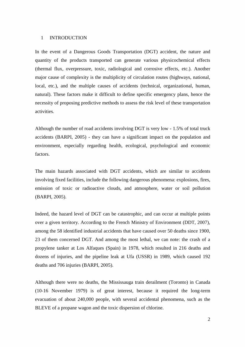
Paris is located in the north-bending arc of the river Seine (Figure 1), includes two
islands which form the oldest part of the city, and is bordered by two outlying parks
(“Bois de Boulogne” and “Bois de Vincennes”).
Figure 1: map of Paris.
Finally, because it is a capital and also the largest French city, Paris features many
important and heterogeneous high-stake sites, whose sensitivity must therefore be
considered in the risk studies.
2.3 The proposed modeling procedure
2.3.1 Generalities
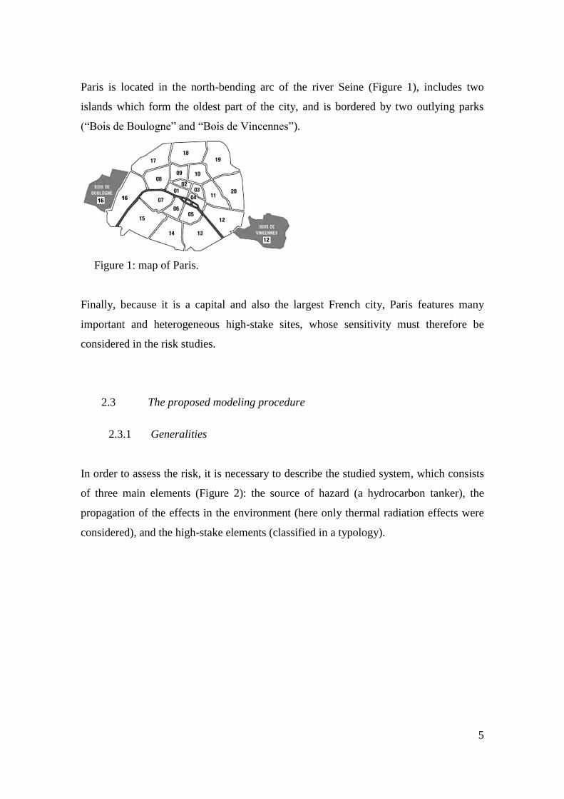
In order to assess the risk, it is necessary to describe the studied system, which consists
of three main elements (Figure 2): the source of hazard (a hydrocarbon tanker), the
propagation of the effects in the environment (here only thermal radiation effects were
considered), and the high-stake elements (classified in a typology).
6
Figure 2: schematization of the studied system.
The risk level thus results from the contribution of two indexes:
- The accident severity, which takes into account the intensity of consequences,
the accident frequency of a DGT and the rate of road accidents;
- The vulnerability of the high-stake elements along the hydrocarbon supply
routes (Tixier et al. 2003).
So, the definition of the risk level (RL) is:
RL = f (Severity, Vulnerability)
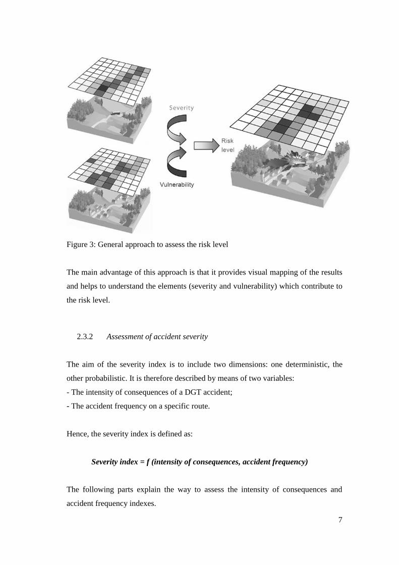
In order to calculate these two main indexes, which are necessary to assess the risk
level of a territory, spatial discretization must be performed. This principle can be
applied using a geographic mesh composed of a set a cells (Figure 3) which have a
specific size determined in function of the precision of the data used and the impact
areas of accidental phenomena. For each cell, each index can be calculated in order:
the severity, then the vulnerability, and finally the risk level. The first two indexes
are normalized using a specific scale in order to assess the risk.
7
Figure 3: General approach to assess the risk level
The main advantage of this approach is that it provides visual mapping of the results
and helps to understand the elements (severity and vulnerability) which contribute to
the risk level.
2.3.2 Assessment of accident severity
The aim of the severity index is to include two dimensions: one deterministic, the
other probabilistic. It is therefore described by means of two variables:
- The intensity of consequences of a DGT accident;
- The accident frequency on a specific route.
Hence, the severity index is defined as:
Severity index = f (intensity of consequences, accident frequency)
The following parts explain the way to assess the intensity of consequences and
accident frequency indexes.

8
2.3.2.1 Intensity of consequences
The intensity of consequences index (IC) takes into account the deterministic
dimensions and the characteristics of accident scenarios. The IC of an accident is
evaluated by the definition of effect areas which are based on specific thresholds
defined in function of the type of high-stake element.
In order to define these effect areas, two sets of thresholds are used (MEDD, 2005):
one for human stakes and another one for environmental and infrastructural stakes. It
is important to call to bear in mind that DGT fire accidents involving hydrocarbons
will impact the territory over no more than some hundreds of meters in most cases.
The first set for human stakes contains the following thresholds (Figure 4):
- 3kW/m², irreversible effect threshold for the definition of the area of
significant hazard to life;
- 5kW/m², lethal effect threshold for the definition of the area of great hazard
to life;
- 8kW/m², significant lethal effect threshold for the definition of the area of
very great hazard to life.
Figure 4: Intensity of consequences of a DGT on a road section.
The second set for environmental and infrastructural stakes consists of the following
thresholds:

9
- 5kW/m²: threshold of significant broken windows;
- 8kW/m²: threshold of serious damage to infrastructures;
- 16kW/m²: threshold of very serious damage to infrastructures, apart from
concrete;
- 20kW/m²: threshold of serious damage to concrete infrastructure;
- 200kW/m²: threshold of catastrophic damage to concrete for at least 10
minutes.
For each of these areas, an index value between 0 and 5 is assumed, as summarized in
the following table:
Thermal radiation
thresholds
Severity index for
human stakes
Severity index for
environmental and
infrastructural stakes
3 kW/m² 1 NA
5 kW/m² 3 1
8 kW/m² 5 2
16 kW/m² NA 3
20 kW/m² NA 4
200 kW/m² NA 5
Beyond the distances obtained for human stakes with a threshold of 3kW/m² and for
environmental and infrastructural stakes of 5kW/m², the value of severity is null (NA)
by assumption.
In order to finalize the severity index, it is necessary to incorporate the accident
frequency dimension.
2.3.2.2 Accident frequency
The accident frequency index is based on the flow rate of DGT per year (Flux_DGT),
the length of the road (L in km) and the accident rate (RA in % per km).

10
The accident frequency index (that is to say the number of DGT accidents per year), for
one section of road, is calculated as:
Accident frequency = L * RA * Flux_DGT
Range of accident frequency Index of accident frequency
10-8
> accident frequency 1
10-7
< accident frequency < 10-8
2
10-6
< accident frequency < 10-7
3
10-5
< accident frequency < 10-6
4
accident frequency > 10-5
5
2.3.2.3 Assessment of the severity index of a route
In order to obtain the value of the severity index of one mesh, it is necessary to take into
account all the contributions provided by each road. So, the severity index of one mesh
is calculated by the sum of each contribution from each road, knowing that a road is
defined by its length, its rate of accidents and finally its DGT flow.
Severity indexmesh = ∑(1 to n) Consequence intensityi * accident frequencyi
with i representing the number of roads influencing the mesh. In another words, the
mesh undergoes the influence of n roads in term of consequence intensity and accident
frequency in function of areas of effect defined by thresholds.
2.3.3 Assessment of the vulnerability of high-stake elements
2.3.3.1 Research question
The aim of the vulnerability index is to assess the danger to high-stake elements if
exposed to a potential hazard. To reach this goal, the critical or sensitive elements

11
within the territory must be identified, geolocated and weighted to assess their relative
importance (Tixier et al. 2012). The idea developed is to identify and characterize the
vulnerability of the elements located in the surroundings of a DGT route. The following
figure summarizes the problem, which aims to answer the following question: is Area
#1, which contains human, environmental and infrastructural high-stake elements, more
or less vulnerable than Area #2, which also contains human, environmental and
infrastructural high-stake elements, but different in quantity and nature?
Figure 5: question of the definition of vulnerability.
To answer this question, it is necessary to characterize the study area (see “3.1. Data and
Databases used”), then to define the stakes. A specific methodology for the assessment
of the vulnerability, based on the work performed during the European project
ARAMIS (Tixier, 2006), can be used. This methodology includes a semi-quantitative
approach (a multicriteria decision method named the “Saaty Method”) which depends
on expert judgments. The analytical hierarchical process (AHP) can be used for
multicriteria assessment problems (Marinoni et al., 2011) in order to score global
objectives in an easy way by including the judgments of stakeholders or other key
people (Zerger et al., 2011). This provides a broad-based representative view of expert
opinion concerning a studied domain (Chen et al., 2011). The main criticism of the AHP
approach is due to the “rank reversal phenomenon” which can lead to a change in the
ranking of two options when a new one is include (DCLG, 2009; Zerger et al., 2011).
We must therefore ensure that the choice of options used to describe the risk ranking
system is exhaustive.

12
2.3.3.2 Saaty multicriteria decision method
The purpose of the Saaty method is to assess priorities. To this end, the first point is to
have a consensus regarding the objective, and secondly to break down the complex and
unstructured situation into its main components. The types of results can be a
classification, the allocation of numerical values regarding subjective judgments, or the
aggregation of judgments to determine the criteria with the highest priorities. The
multicriteria hierarchical method enables decision-making by a group in a consensual
way due to a better coherence of judgments, through the construction of a linear
additive model (Chen et al. 2011).
Saaty’s multicriteria hierarchical method (Saaty, 1984) is based on four main steps:
- A description of the studied system (some elements and criteria are proposed in order
to characterize the situation);
- The construction of hierarchies (to organize the elements and the criteria to respond to
the question);
- An assessment of priorities (based on expert judgments);
- Validation of coherence.
The construction of a hierarchical structure requires the creation or identification of
links between the various levels of that structure.
Each element or criteria of a hierarchical structure is situated at a given level of the
structure. The upper level corresponds to the global objective (or dominant element).
The elements of a given level are ranked by binary comparison according to their
impact on an element at the next highest level, in order to the elements. The various
levels of a hierarchy are, consequently, interconnected.
A complex situation can be analyzed by a systematic approach with the help of such a
hierarchical structure. The priorities have to be assessed. This process is performed by
comparing elements two-by-two (binary comparison). This ranks the elements
according to their relative importance. Finally, the logical coherence of the structure is
13
validated to confirm the whole applied process. To make the binary comparisons, it is
necessary to use a scale based on standard numerical variables or more qualitative
variables that help to take into account qualitative aspects.
From this definition and from hierarchical structures, the matrices and functions of the
vulnerability index are deduced. The matrices are translated into a questionnaire which
enables experts’ judgments to be gathered for the evaluation of each coefficient of the
vulnerability functions.
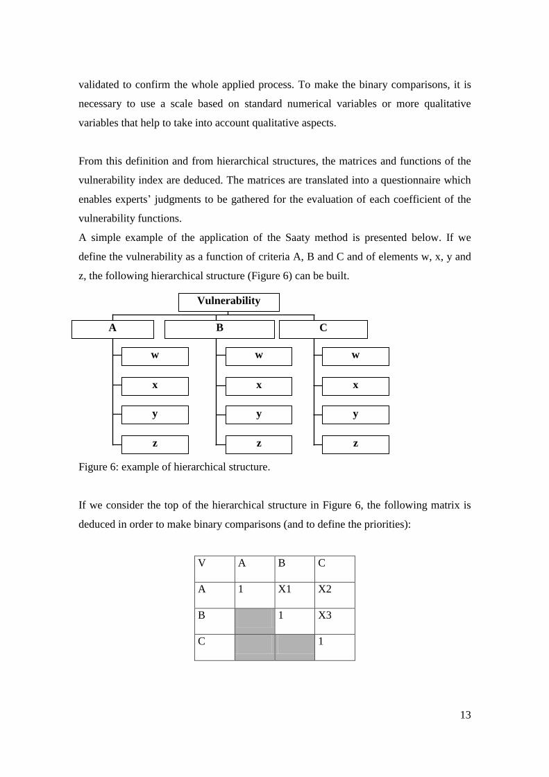
A simple example of the application of the Saaty method is presented below. If we
define the vulnerability as a function of criteria A, B and C and of elements w, x, y and
z, the following hierarchical structure (Figure 6) can be built.
Figure 6: example of hierarchical structure.
If we consider the top of the hierarchical structure in Figure 6, the following matrix is
deduced in order to make binary comparisons (and to define the priorities):
V A B C
A 1 X1 X2
B 1 X3
C 1
Vulnerability
A B C
w w w
x
y
z
x
y
z
x
y
z

14
where X1, X2 and X3 are the weighting factors provided by experts through a
questionnaire. The questionnaires are analyzed by inverse methods to retrieve the
weighting factors. From this matrix, eigenvectors can be calculated and named , and
. In another words, each of these values gives the relative importance of each criterion.
The vulnerability (V) is thus a function of the vulnerability criteria A, B and C.
V = A + B + C
With , and , the vulnerability factors of the vulnerability function.
A specific processing operation was required to aggregate the experts’ judgments. Each
judgment was aggregated by the use of the geometrical mean. A single questionnaire
was thus obtained, which was an aggregation of the judgments of all the experts
consulted. All the judgments are added to the matrices and the vulnerability factors
assessed as presented below.
In order to validate the vulnerability factors, the Consistency Ratio (CR) is assessed and
must be less than 10%.
CR = (CI) / (RI).
Where
CI is the Consistency Index, with CI = (λmax - n) / (n-1) and n the number of compared
elements.
λmax. is the maximum eigenvalue (Perron root) of the matrix.
RI = Random Index. For each matrix of size n, Saaty’s team generated random matrices
and computed their mean CI value and called it the Random Index.
2.3.3.3 Study area and high-stake element typologies
The aim of this section is to define the territory subject to DGT hazard in order to
determine the risk level. It is therefore necessary to propose a set of types of high-stake
element so as to accurately characterize the environment. It is necessary to find the right

15
balance between the number of site-types to be taken into account and the limitations
due to the multicriteria decision method.
First of all, sites were divided into three categories in function of the stakes involved,
and each of them detailed in a list of generic types of high-stake element:
- Human (H)
o Private dwelling (H1)
o People present in a public assembly building (H2)
o Users of communication networks (H3)
- Environmental (E)
o Agricultural area (E1)
o Natural area (E2)
o Specific natural area (E3)
o Wetland or water body (E4)
- Infrastructural (I)
o Industrial site (I1)
o Public utility or infrastructure (I2)
o Private structure (I3)
o Public structure (I4)
As described above, Saaty’s multicriteria hierarchical method (Saaty, 1984) is based
on three main steps, once a system has been described:
- construction of hierarchies;
- assessment of priorities;
- validation of coherence.
The construction of a hierarchical structure requires the creation or the identification
of links between the various levels of this structure. In order to have a good
understanding of the situation, the description of the environment is completed by a
typology of impacts due to exposure to thermal radiation. Three impacts due to
thermal radiation are considered to characterize the effects of major accidents on
high-stake element:

16
- Integrity impact, which respectively qualifies the human, environmental and
infrastructural damage;
- Economic impact which qualifies an effect in terms of loss of production or
of rehabilitation;
- Psychological impact which qualifies an effect in terms of influence on a
group of people.
It is then necessary to organize these typologies in order to respond to the
vulnerability question. The next step therefore consists in structuring the information
in accordance with the following definition of the vulnerability: the vulnerability of
each type of high-stake element in function of thermal radiation effect is evaluated
by binary comparison using the three impact types as characterization criteria.
The result is the vulnerability of one class of high-stake element to a thermal
radiation effect. The associated hierarchical structure for human vulnerability is
presented in Figure 7. In this hierarchical structuration, each category of human
element is compared in function of each criterion (integrity, economic and
psychological impact).
Figure 7: hierarchical structure for human vulnerability.
The same hierarchical structure applies to environmental and infrastructural
vulnerability. The matrices and functions of the vulnerability index are deduced from
this definition and the hierarchical structures. The matrices are translated into a
questionnaire which helps to collect the expert judgments for the evaluation of each
vulnerability coefficient of the vulnerability functions.

17
Thirty eight experts had already been individually consulted during the ARAMIS
European project (Tixier et al., 2006). The breakdown of experts by type is presented
in Figure 8: about 60 % were risks experts (from public or private organizations),
while the remaining 40% were industrialists or local authority employees.
Figure 8: Breakdown of experts by type.
A specific processing operation was performed to aggregate the judgments of the
above-mentioned experts. Each judgment was aggregated by means of the
geometrical average, producing a new questionnaire which is the aggregation of the
judgments of all the experts consulted. All the assessments obtained were assessed
into the matrices and the vulnerability factors could be assessed. The results are
given in the next paragraph.
To assess the vulnerability factors of each function, the eigenvectors of the matrixes
must be calculated. The results correspond to the factors of vulnerability and we can
see that all the Consistency Ratios (CR) have a value lower than 10%. The following
table presents the results for the human, environmental and infrastructural
vulnerability functions.
Human vulnerability – thermal radiation CR %
VHft = 0,648 VHftS + 0,122 VHftE + 0,230 VHftP 0.3
VHftS = 0,548H1 + 0,249H2 + 0,203H3 1
VHftE = 0,593H1 + 0,268H2 + 0,139H3 0.86
VHftP = 0,400H1 + 0,400H2 + 0,200H3 0

18
Environmental vulnerability – thermal radiation
VEft = 0,550 VEftS + 0,240 VEftE + 0,210 VEftP 1.58
VEftS = 0,195E1 + 0,231 E2 + 0,426E3 + 0,148E4 2.54
VEftE = 0,227E1 + 0,227 E2 + 0,424E3 + 0,122E4 0.57
VEftP = 0,200E1 + 0,200 E2 + 0,400E3 + 0,200E4 0
Infrastructural vulnerability – thermal radiation
VIft = 0,443 VIftS + 0,387 VIftE + 0,169 VIftP 1.58
VIftI = 0,246I1 + 0,298I2 + 0,21I3 + 0,246I4 3.36
VIftE = 0,400I1 + 0,200I2 + 0,200I3 + 0,200I4 0
VIftP = 0,142I1 + 0,286I2 + 0,286I3 + 0,286I4 0
2.3.3.4 Quantification factors
The quantification factors determine the level of stakes in the study area. A
quantification factor is defined as a dimensionless variable, assuming values in the
range 0-1, where 0 indicates the absence of the stake in the area and 1 indicates that
the quantity of this stake in the area reaches its expected maximum.
2.4 Development scheme
2.4.1 Global use cases
In a preliminary study, the actors and interactions of the system were defined in order to
construct the messages intended to be exchanged with the users. These specifications
were further refined using various UML (Unified Modeling Language) models. As
shown in Figure 9, the following four fundamental steps can be identified as being
required:
- The manual selection of a road route (1): the user first selects a sequence of
road segments which can be considered as a route for the hydrocarbon transportation;
- The generation of an analysis grid to cover the study area (3): square cells are
created in order to divide the environment into a set of meshes. The spatial analysis can
be made more or less precise by adjusting the size of each mesh;

19
- Cross-analysis (territory assessment) of the grid with other layers of the
Geographic Information System (4): the properties of each object covered by a mesh are
aggregated and associated to the mesh;
- Thematic analysis for viewing the results (6): this step displays the results from
a human, infrastructural or environmental point of view, with an absolute or relative
scale of view.
Figure 9: dynamic context diagram of the tool.
The tool uses a batch processing operation (Step 3, Figure 9) to schedule and automate a
set of operations and computations which form its kernel. Several difficulties occurred
during the software modeling and development: the main ones are detailed in the
following section through some of the implemented algorithms.
2.4.2 Quick survey of the main algorithms implemented in the kernel
2.4.2.1 Grid creation process
The method selected for creating the grid is recursive construction of each cell, as
shown in Figure 10. The size choice for the cells depends on the following two

20
constraints: the accuracy of the geography database and the distances of thermal
radiation effects for the studied hazard scenarios (see Section 2.3.2). By assumption, we
set up a size of 50 meters for the cells of each grid.
Figure 10: generation grid algorithm.
The primary focus is in fact to choose between the two main possible strategies in order
to cover a territory with an analysis grid made up of square meshes.
The first one consists in the creation of a simple rectangular grid for all the studied
territory (here, the city of Paris) thanks to a basic algorithm based on a variable which
increments the rows/columns indexes to add each cell. This common approach can be
implemented simply and quickly but the high number of meshes potentially created for
an extended territory and which have to be crossed with GIS layers may cause
significant time problems in the subsequent computational processes.
The second one only deals with the geographical areas of interest (here, the road
sections plus the distances of thermal effects). It is thus possible to improve the
processing time, but this approach requires a specific algorithm to cover only the
targeted parts of the territory.
Therefore, it can be suggested to operate all road sections with the following sequential
process: creation, georeferencing, union into a unified grid. In the existing data, each
road section is a polyline object which can be composed of several linear segments.
Each section of a given road is split into unitary segments which are covered by

21
intermediates sets of meshes. The created cells can be unified when all segments of all
sections of all studied roads are processed. The following figure summarizes the
mechanism as it was conceived during this design phase.
Figure 11: first algorithm tested.
2.4.2.2 Coverage problem and clipping solution
However, a coverage problem occurred in the meshing of many routes due to their self-
structure. In fact, these objects are defined as polylines in order to describe the road
network. Figure 12 shows the benchmarks, i.e. the starting and the ending points, used
in the meshing process of a road section,.
Figure 12: coverage problem of the first meshing algorithm.

22
This problem was solved by improving the first algorithm in order to browse (temporary
clipping) each unitary segment (single line) of each road section (polyline). For the rest,
the initial principle was retained (Figure 13).
Figure 13: the two main mechanisms of the second meshing algorithm.
2.4.2.3 Homogeneity problem and magnetic arrangement
Nevertheless, new unexpected results concerning the grids’ homogeneity occurred.
With the method employed, each mesh was generated by following the direction of its
associated road segment, which meant that the cells were not drawn using the same
reference points (Figure 14).
Figure 14: homogeneity problem of the second meshing algorithm.
In order to solve this problem, we created a specific method named “magnetic
arrangement” in order to set all meshes in the same orthonormal basis. But this
approach resulted in a final problem, as shown in Figure 15 below.

23
Figure 15: continuity problem between magnetized grids.
2.4.2.4 Continuity problem and enhanced magnetic arrangement
To correct this lack of continuity, we had to set up a unified magnetic grid (we
developed a method named “enhanced magnetic arrangement”) to calibrate each
intermediate mesh with its neighbors in order to finally obtain a uniform continuous set
of meshes. Figure 16 shows the mechanism used for the grid calibration.
Figure 16: “enhanced magnetic arrangement” of two sets of meshes.
Figure 16 highlights furthermore the inevitable presence of repetitions (grayed cells):
the ending point of a segment may also be the starting point of another one. These
specific cells located at the ends of road segments can be removed by a method which
we developed to verify the unicity of the individual elements making up the grid.
3 SOFTWARE
3.1 Data and Databases used
The first step in the work consisted in describing the expected data. It aim was to define
which inputs will be used in the risk assessment model and the index calculation
24
processes for one or several routes selected by the user. The cartographic data required
are:
- A description of the typology of the human, infrastructural, environmental
high-stake elements present in the study area;
- A recent census of the population;
- A road network with traffic data specific to DGT, and accident rates.
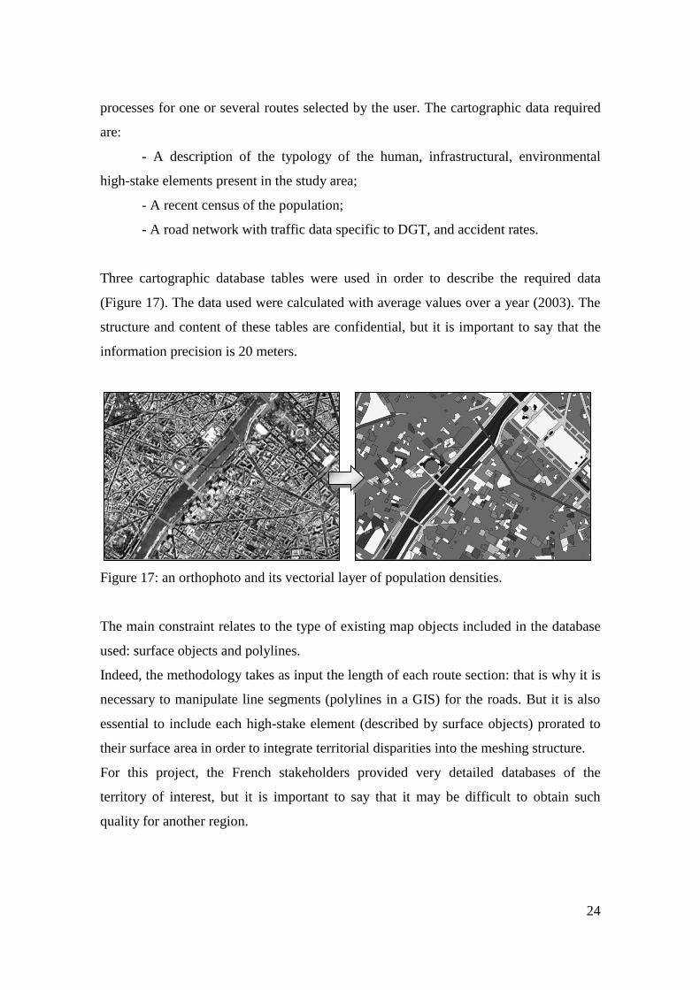
Three cartographic database tables were used in order to describe the required data
(Figure 17). The data used were calculated with average values over a year (2003). The
structure and content of these tables are confidential, but it is important to say that the
information precision is 20 meters.
Figure 17: an orthophoto and its vectorial layer of population densities.
The main constraint relates to the type of existing map objects included in the database
used: surface objects and polylines.
Indeed, the methodology takes as input the length of each route section: that is why it is
necessary to manipulate line segments (polylines in a GIS) for the roads. But it is also
essential to include each high-stake element (described by surface objects) prorated to
their surface area in order to integrate territorial disparities into the meshing structure.
For this project, the French stakeholders provided very detailed databases of the
territory of interest, but it is important to say that it may be difficult to obtain such
quality for another region.

25
3.2 General algorithm
The main process implemented is based on four steps:
- The manual selection of a set of routes (one or more roads) by the user;
- The automatic generation of an analysis grid along this route;
- The cross-analysis between the grid and the GIS layers;
- The assessment of the risk for DGT.
The risk assessment step uses at the same time the high-stake element typology defined
by the methodology and a grid. Figure 18 illustrates the cross-analysis operation
between a grid and GIS layers in order to extract the expected data.
Figure 18: illustration of the cross-analysis between a set of meshes and GIS layers.
The process is designed like a transverse mechanism associating information about the
human, infrastructural and environmental stakes into each mesh. All data are calculated
taking into account the size and the area of meshes (densities of surface objects,
proportional lengths of polylines). Subsequently, the results are stored in the GIS table
which contains the analysis grid (MapInfo file format).
3.3 GIS-based tool “CARTENJEUX”
The final tool implemented to study hydrocarbon supply routes was based on a
Geographical Information System. This software named CARTENJEUX, which means
“stakes-based mapping” in French (figure 19), is in the form of an add-on (Ayral, 2010)
which aims to assess human, infrastructural and environmental risk.

26
Figure 19: welcome page of the software.
3.4 Route selection
In order to study a route through grid analysis, it is necessary first to select linear
objects directly on the GIS road layer. This solution has the advantage of being visual
and concrete for the user since it physically indicates the road segments with which
he/she wants to work. That is why the selection tools available in MapInfo are very
useful because they offer a varied panel of possible selections of linear objects (for
example, road sections).
3.5 Grid generation
Once a set of road segments has been made up, the user can configure a mesh size (in
meters) for the grid building and a dimension (also in meters) on both sides of the axis,
indicating the spreading of the grid around the road axis. This last distance is obtained
in function of effects thresholds and can be entered by leans of a specific user-friendly
interface for the grid generation settings. Users hence have the capability of changing
the size of the grid at run time.
It is important to say that the tool allows the user to manage a set of grids. Indeed, it is
possible to display two routes currently loaded in memory in order to compare them.
When several grids are shown simultaneously, the user can select one of them in order
to choose the set of meshes on which the next operations will be done (statistics for
example).
27
At this stage, the generation parameters are validated and the program starts the
construction of the grid. As a result, the meshes created are aggregated in a unified grid,
ready to be used to assess the risk of the covered territory.
3.6 Cross-analysis of the grid with stakes layers
A dynamic grid is now created and saved in a specific MapInfo table, whose fields are
empty. This table has both upper and lower bounds, and all the cells of the grid are
contiguous within those bounds.
So, the risk assessment process consists of cross-analysis, iterating all the cells objects
in order to aggregate them with the data layers opened in MapInfo.
In the end, all the table’s fields are assigned by quantification factors about each class of
stakes.
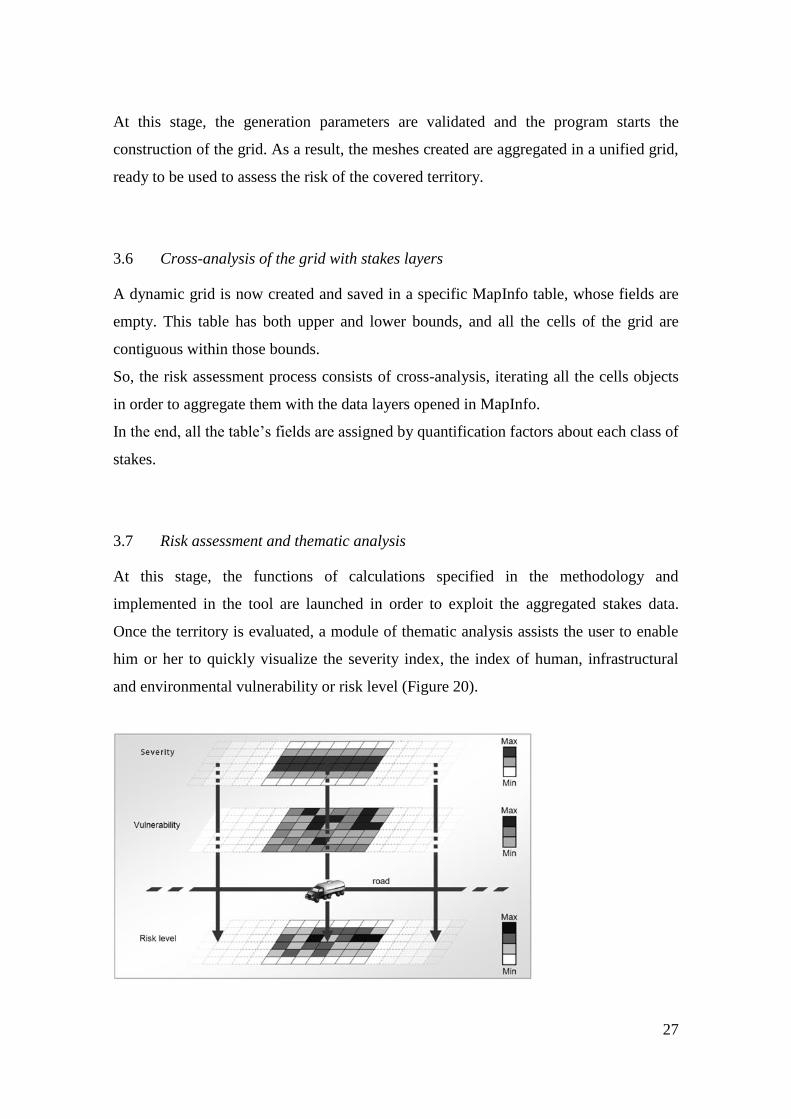
3.7 Risk assessment and thematic analysis
At this stage, the functions of calculations specified in the methodology and
implemented in the tool are launched in order to exploit the aggregated stakes data.
Once the territory is evaluated, a module of thematic analysis assists the user to enable
him or her to quickly visualize the severity index, the index of human, infrastructural
and environmental vulnerability or risk level (Figure 20).

28
Figure 20: the three data layers mappable by CARTENJEUX.
In fact, this module is equivalent to a thematic map browser which proposes standard
scales of visualizations (relative or absolute) in a few mouse-clicks. The user is thus
able to obtain several maps about the severity of a potential accident, the vulnerability
of high-stake elements, and the different levels of risk of the initial DGT route.
4 RESULTS AND DISCUSSION
It is important to say that the exact location of hydrocarbon tanks and the precise supply
routes are sensitive and therefore confidential. The examples presented in the following
sections are fictive, and any similarity to actual routes would be purely coincidental.
4.1 Overview
In order to illustrate the results given by the cartographic tool CARTENJEUX, this part
shows an example (Figure 21) of two possible supply routes (named route 1 and route
2) between an hydrocarbon tank and a gas station (respectively named A and B). The
objective is to compare the risk of the two routes from a human, environmental and
infrastructural point of view, thanks to spatial and statistical results. This first example
is just theoretical because the real supply routes chosen by French stakeholders are
confidential.

29
Figure 21: two possible routes between A and B (left) with their analysis grids (right).
Two grids are automatically created by the developed routines around each road axis.
The different assessments will be run later, in order to obtain a map of risks. Figure 21
shows the two study areas before the cross-analysis.
In a last step, the analysis begins and displays the spatial results. Figure 22 indicates the
human vulnerability in the surroundings of the two chosen routes. It is possible to see
directly many disparities thanks to the use of cells which enable the consideration of one
particular high-stake element group. A function is also available to specify the
transparency of the grid in order to consult the subjacent layers and the thematic
analysis simultaneously.

30
Figure 22: human vulnerability around two routes.
The dark gray cells indicate the presence of critical human high-stake elements which
are due to highly urbanized areas.
In order to compare more precisely the two routes, the cartographic tool produces a
statistical index of risk, as shown in the following figure. Indeed, the user can compare
the evolution of the human, infrastructural and environmental risk levels (RL).
Route #1 Route #2
Human RL 23 % Human RL
Environmental RL 65% Environmental RL
Infrastructural RL 3 % Infrastructural RL
Figure 23: evolution of the statistical index of risk between two supply routes.
In this example, the first route presents the lowest environmental risk level, whereas the
second one leads to a decrease in the human and infrastructural risk levels. Thereby, this
synthesis approach helps the user to understand the impacts of the two possible supply
routes: in a highly urbanized area and if the environmental stakes are not overriding, the
second route may be preferred.
In the previous figure, the main differences between the two routes were the human and
environmental risks. The move from 1 to 2 would involve a reduction of 23% for the
human stakes risk and a rise of 65% for the environmental ones. With regard to the
infrastructural stakes, the analysis shows there is a light reduction in vulnerability of
3%.
4.2 Further details
The accuracy of the cartographic data led to an analysis of a cell size in order to obtain a
fair compromise for mitigating the error factor during the meshing process of the road

31
network. Accordingly to the geometric precision of the database (about 20 meters), a
cell width of 50 meters was validated.
With the help of CARTENJEUX, different kind of maps can be obtained. The following
examples (figures 24, 25, 26) concern several routes of supply for which the severity,
the vulnerability and the global risk has been quantified. This analysis concerns all the
territory of “Ile de France”, but only an extract of the results is presented for reasons of
confidentiality.
Figure 24: map of the severity index.

32
Figure 25: map of environmental vulnerability.

33
Figure 26: map of environmental risk.
The example shown below (Figure 27) is located south of the “Bois de Vincennes”,
along a highway, near the Seine. The human risk around the highway section is
calculated (on the bottom right) and CARTENJEUX gives the possibility for the user to
consult both the severity index (top right) and the human vulnerability (middle right).
34
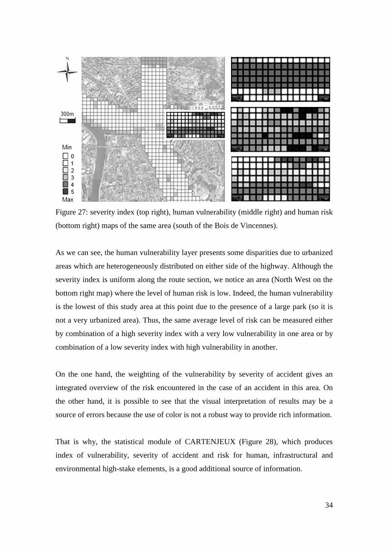
Figure 27: severity index (top right), human vulnerability (middle right) and human risk
(bottom right) maps of the same area (south of the Bois de Vincennes).
As we can see, the human vulnerability layer presents some disparities due to urbanized
areas which are heterogeneously distributed on either side of the highway. Although the
severity index is uniform along the route section, we notice an area (North West on the
bottom right map) where the level of human risk is low. Indeed, the human vulnerability
is the lowest of this study area at this point due to the presence of a large park (so it is
not a very urbanized area). Thus, the same average level of risk can be measured either
by combination of a high severity index with a very low vulnerability in one area or by
combination of a low severity index with high vulnerability in another.
On the one hand, the weighting of the vulnerability by severity of accident gives an
integrated overview of the risk encountered in the case of an accident in this area. On
the other hand, it is possible to see that the visual interpretation of results may be a
source of errors because the use of color is not a robust way to provide rich information.
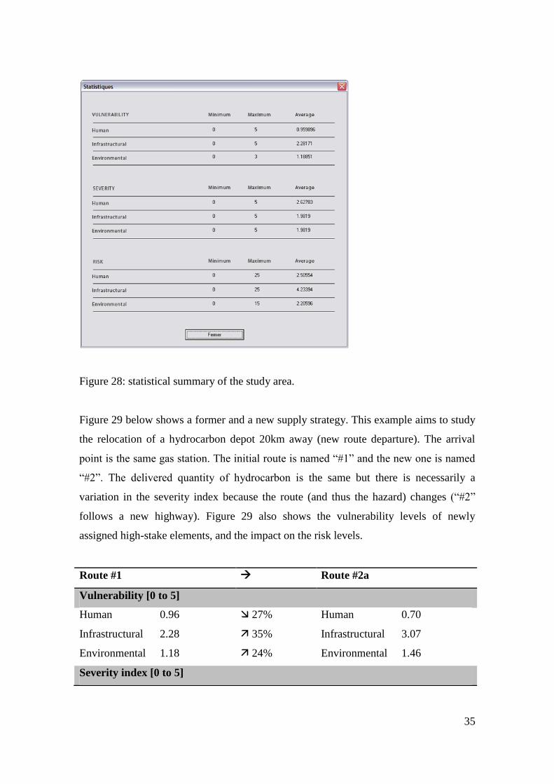
That is why, the statistical module of CARTENJEUX (Figure 28), which produces
index of vulnerability, severity of accident and risk for human, infrastructural and
environmental high-stake elements, is a good additional source of information.
35
Figure 28: statistical summary of the study area.
Figure 29 below shows a former and a new supply strategy. This example aims to study
the relocation of a hydrocarbon depot 20km away (new route departure). The arrival
point is the same gas station. The initial route is named “#1” and the new one is named
“#2”. The delivered quantity of hydrocarbon is the same but there is necessarily a
variation in the severity index because the route (and thus the hazard) changes (“#2”
follows a new highway). Figure 29 also shows the vulnerability levels of newly
assigned high-stake elements, and the impact on the risk levels.
Route #1 Route #2a
Vulnerability [0 to 5]
Human 0.96 27% Human 0.70
Infrastructural 2.28 35% Infrastructural 3.07
Environmental 1.18 24% Environmental 1.46
Severity index [0 to 5]

36
Human 2.62 16% Human 2.20
Infrastructural 1.98 25% Infrastructural 1.47
Environmental 1.98 10% Environmental 1.79
Risk level [0 to 25]
Human 2.52 39% Human 1.54
Infrastructural 4.51 = Infrastructural 4.51
Environmental 2.33 12% Environmental 2.61
Figure 29: comparison of two supply strategies.
The different stakes located along the two routes lead to heterogeneous levels of
vulnerability. But, because “#2” is more secure than “#1”, this strategy reduces the risks
of a road accident and thus leads to a decrease in the severity index.
We see with this hypothetical case that level of human risk decreases while the risk
levels for the environment increases. The weighting factors of the methodology, which
integrate the rise in infrastructural vulnerability and the reduction in the severity index
for the same stakes, indicate that there is no change in the infrastructural levels of risk.
5 CONCLUSIONS
The project consists in the development of a predictive model for determining whether
increasing the flow of hydrocarbon transportation (consequence of relocations)
significantly increases risk (for people, infrastructure and the environment) and by how
much.
The major contribution of this work is to provide a structured proposition for assessing
risk levels using severity and vulnerability indexes depending on the location of a DGT
accident. A GIS-based tool implements a structured methodology which is proposed to
assess the risk levels of supply routes by determining the severity index, the territorial
vulnerability and the risk level. The quantification of the vulnerability of the high-stake
elements, combined with the severity index of the hydrocarbon transportation gives the
associated risk level. In order to implement the proposed methodology, a development
scheme is proposed. On this basis, the identified functionalities are implemented by way

37
of specific routines to build a grid analysis and to run optimized GIS queries. The result
is an integrated user friendly tool named CARTENJEUX. Although the methodology
was calibrated for studies in “Ile de France” (including Paris), this operational software,
based on a geographical information system, might be applied to another territory or
further studies. Decision makers can produce three kinds of thematic maps
(vulnerability, severity of accident and risk level) for human, infrastructural and
environmental stakes. A statistical module gives also another vision of the results in
order to manage risks. CARTENJEUX thus helps to determine the most preferable route
for hydrocarbon DGT.
Using the developed GIS-tool, French stakeholders were able to consider the issues
globally and achieve better management of DGT in the “Ile de France” region.
ACKNOWLEDGMENTS
The authors would like to thank the French ministry of industry (DGEMP) for
supporting this research.
REFERENCES
Ayral P-A., Sauvagnargues-Lesage S., Tena-Chollet F., Thierion V., 2010, “Les
Systèmes d’Information Géographique : mise en œuvre”, Les Techniques de
l’Ingénieur, 14p, réf. H7416.
BARPI, 2005, “Bilan des accidents technologiques 1992-2004”, Bureau d'Analyse des
Risques et Pollutions Industrielles: 19p, in French.
Bubbico R., Di Cave S., Mazzarotta B., 2004, “Risk analysis for road and rail transport
of hazardous materials: a GIS approach”, Journal of Loss Prevention in the Process
Industries, Vol 17, Issue 6, pages 483-488.

38
Bubbico R., Maschio G., Mazzarotta B., Milazzo M. F., Parisi E., 2006, “Risk
management of road and rail transport of hazardous materials in Sicily”, Journal of Loss
Prevention in the Process Industries, Volume 19, Issue 1, pages 32-38.
Chen H., Wood M.D., Linstead C., Maltby E., “Uncertainty analysis in a GIS-based
multi-criteria analysis tool for river catchment management”, Environmental Modelling
& Software, Volume 26, Issue 4, April 2011.
Dandrieux A., Heymes F., Tixier J., Lecysin N., Tena-Chollet F., Spinelli R., Slangen
P., Hodin A., Munier L., Lapébie E., Le-Gallic C., Dusserre G., “An integrated
methodology research to determine consequences of a vessel destruction”, ESREL
2006, Safety and Reliability for Managing Risk 18-22 September 2006 – Estoril,
Portugal, p.1965-1972.
DCLG (Department for Communities and Local Government), “Multi-criteria analysis:
a manual”, London, 2009.
DDT, 2007, “Risque transport de matières dangereuses”, Direction Départementale des
Territitoires de la Loire, in French.
Fabiano B., Currò F., Palazzi E., Pastorino R., 2002, “A framework for risk assessment
and decision-making strategies in dangerous good transportation”, Journal of Hazardous
Materials, Vol 93, Issue 1, 1, pages 1-15.
Marinoni O., Adkins P., Hajkowicz S., “Water planning in a changing climate: Joint
application of cost utility analysis and modern portfolio theory”, Environmental
Modelling & Software, Volume 26, Issue 1, January 2011.
MEDD, 2005, “Arrêté du 29 septembre 2005 relatif à l'évaluation et à la prise en
compte de la probabilité d'occurrence, de la cinétique, de l'intensité des effets et de la
gravité des conséquences des accidents potentiels dans les études de dangers des
installations classées soumises à autorisation”, legiFrance.

39
Milazzo M.F., Lisi R., Maschio G., Antonioni G., Bonvicini S., Spadoni G., 2002,
“HazMat transport through Messina town: from risk analysis suggestions for improving
territorial safety”, Journal of Loss Prevention in the Process Industries, Vol 15, Issue 5,
pages 347-356.
Milazzo M.F., Lisi R., Maschio G., Antonioni G., Spadoni G., “A study of land
transport of dangerous substances in Eastern Sicily”, Journal of Loss Prevention in the
Process Industries, 23(3): 393-403, 2010.
Oggero A., Darbra R.M., Munoz M., Planas E., Casal J., 2006, “A survey of accident
occurring during the transport of hazardous substances by road and rail”, Journal of
Hazardous Materials, Vol 133, Issue 1-3, pages 1-7.
Saaty T. L., 1984, “Décider face à la complexité : une approche analytique multicritère
d’aide à la décision”, collection université – entreprise, entreprise moderne d’édition,
Paris.
Tixier J, Dandrieux A, Dusserre G, Bubbico R., Mazzarotta B., Silvetti B., Hubert E.,
Rodrigues N., Salvi O., 2006, “Environmental vulnerability assessment in the vicinity
of an industrial site in the frame of ARAMIS European project”, Journal of Hazardous
Materials, Vol 130, Issue: 3, pages: 251-264.
Tixier J, Dusserre G, Salvi O, et Gaston D., 2002, “Review of 62 risk analysis
methodologies of industrial plants”, Journal of Loss prevention in the process industries,
Vol 15, Issue: 4, pages: 291-303.
Tixier J., Dandrieux A., Dusserre G., Bubbico R., Luccone L.G., Mazzarotta B., Carta
R., Di Cave S., Silvetti B., Hubert E., Rodrigues N., Salvi O., Gaston D., “Assessment
of the environment vulnerability in the surroundings of an industrial site”, ESREL 2003,
Maastricht 15-18, June 2003.

40
Tixier J., Tena-Chollet F., Munier L., Lapébie E., Le-Gallic C. & Dusserre G.,
“Development of a GIS-based approach for the vulnerability assessment of a territory
exposed to a potential risk”, European Safety, Reliability & Data Association, 2012.
Verma M., “Railroad transportation of dangerous goods: A conditional exposure
approach to minimize transport risk”, Transportation Research Part C: Emerging
Technologies, 19(5):790-802, 2011.
Zerger A., Warren G., Hill P., Robertson D., Weidemann A., Lawton K., “Multi-criteria
assessment for linking regional conservation planning and farm-scale actions”,
Environmental Modelling & Software, Volume 26, Issue 1, January 2011.