development of a snowdrift model with the lattice
TRANSCRIPT

Tanji et al. Prog Earth Planet Sci (2021) 8:57 https://doi.org/10.1186/s40645-021-00449-0
RESEARCH ARTICLE
Development of a snowdrift model with the lattice Boltzmann methodSeika Tanji1* , Masaru Inatsu2,3 and Tsubasa Okaze4
Abstract
We developed a snowdrift model to evaluate the snowdrift height around snow fences, which are often installed along roads in snowy, windy locations. The model consisted of the conventional computational fluid dynamics solver that used the lattice Boltzmann method and a module for calculating the snow particles’ motion and accumulation. The calculation domain was a half channel with a flat free-slip boundary on the top and a non-slip boundary on the bottom, and an inflow with artificially generated turbulence from one side to the outlet side was imposed. In addition to the reference experiment with no fence, experiments were set up with a two-dimensional and a three-dimensional fence normal to the dominant wind direction in the channel center. The estimated wind flow over the two-dimen-sional fence was characterized by a swirling eddy in the cross section, whereas the wind flow in the three-dimen-sional fence experiment was horizontally diffluent with a dipole vortex pair on the leeward side of the fence. Almost all the snowdrift formed on the windward side of the two-dimensional and three-dimensional fences, although the snowdrift also formed along the split streaks on the leeward side of the three-dimensional fence. Our results sug-gested that the fence should be as long as possible to avoid snowdrifts on roads.
Keywords: Drifting snow, Blowing snow, Snow fence, Lattice Boltzmann method
© The Author(s) 2021. Open Access This article is licensed under a Creative Commons Attribution 4.0 International License, which permits use, sharing, adaptation, distribution and reproduction in any medium or format, as long as you give appropriate credit to the original author(s) and the source, provide a link to the Creative Commons licence, and indicate if changes were made. The images or other third party material in this article are included in the article’s Creative Commons licence, unless indicated otherwise in a credit line to the material. If material is not included in the article’s Creative Commons licence and your intended use is not permitted by statutory regulation or exceeds the permitted use, you will need to obtain permission directly from the copyright holder. To view a copy of this licence, visit http://creativecommons.org/licenses/by/4.0/.
1 IntroductionSnowdrifts are patchy accumulations of snow resulting mainly from the redistribution of snow particles on the ground by drifting snow, which is the horizontal move-ment of snow particles by creep and saltation on the sur-face. Snowdrifts can severely affect human activities; for example, snowdrifts in mountainous terrain can trigger avalanches and affect the mass balance of water (Lehning et al. 2006, 2008; Mott et al. 2010; Vionnet et al. 2017). Moreover, snowdrifts cause traffic disruption because vehicles tend to stack and stagnate on roads with a snow depth of 15 cm (Kaneko et al. 2011). Snow fences are one of the solutions to mitigate the problems caused by snow-drifts, especially on roads in snowy, windy locations. Snowdrift distribution around snow fences depends strongly on their design parameters, such as height,
thickness, bottom gap, space between panels, penetration rate of porous fences, and distance from the road (Tabler 1986; Uematsu et al. 1991; Alhajraf 2004). Some stud-ies have examined the onset of drifting snow and snow accumulation in wind tunnel experiments (Delpech et al. 1998; Okaze et al. 2012; Zhou et al. 2014). Other stud-ies have reported the effect of snow fence design on the size of snowdrifts on roads based on field observations (Tabler 1980, 1994; Takeuchi 1980; Takeuchi et al. 1986). However, field observations provide limited opportuni-ties to sample drifting snow events at a certain site, and wind tunnel experiments do not always correspond to real situations owing to scaling effects. Moreover, it is generally costly to obtain sufficient data to design snow fences using these methods. However, the advancement of computer technology has enabled numerical simu-lations of snowdrift development to be performed to search for an optimal snow-fence design at a target site.
Numerical simulations of drifting snow require com-putational fluid dynamics (CFD) and the estimation of
Open Access
Progress in Earth and Planetary Science
*Correspondence: [email protected] Graduate School of Science, Hokkaido University, N10W8, Sapporo 0600810, JapanFull list of author information is available at the end of the article
Page 2 of 16Tanji et al. Prog Earth Planet Sci (2021) 8:57
snowdrift distribution. Numerical simulations of drift-ing snow were pioneered in the 1990s by Uematsu et al. (1991) and Liston et al. (1993). These studies used a wind simulation based on the Reynolds-aver-aged Navier–Stokes equations model with turbulence parameterizations, such as K-theory and the k-ε model. These models reproduced the snowdrift distribution around a simple snow fence. Some studies extended these models to include drifting snow processes due to multiple snow events that were more complicated (Beyers et al. 2004; Tominaga et al. 2011a, 2011b). The large-eddy simulation (LES) has been applied to snow transport simulations to describe turbulence more accurately (Okaze et al. 2018; Wang and Jia 2018). For example, Zwaaftink et al. (2014) combined the LES and a Lagrangian stochastic model and described the tem-poral and spatial variability of drifting snow with their model. Some studies have considered the momentum exchange between particles and background wind (Elg-hobashi 1994). Moreover, turbulent wind is strongly affected not only by the fixed boundaries, including topography and artificial obstacles, but also by snow surfaces that vary temporally due to snowdrifts.
The lattice Boltzmann method (LBM) is a CFD algo-rithm for quick calculations [see McNamara and Zanetti (1988) for an introduction and Benzi et al. (1992), Qian et al. (1995), and Chen and Doolen (1998) for compre-hensive reviews]. In the LBM, the Navier–Stokes equa-tions are replaced with a distribution function equation called the lattice Boltzmann equation that treats the fluid flow as microscopic fictitious particles in the space lattice (Chen et al. 1992; Qian et al. 1992). The lattice Boltzmann equation can be numerically solved by the translation of the distribution function and the relaxation to the equilibrium state. The LBM algorithm is character-ized by simpler implementation and higher efficiency in parallel computation than the conventional CFD algo-rithm (Chen and Doolen 1998). Han et al. (2019) demon-strated that the LBM was three-fold faster than the finite volume method in 16-core parallel processing. The LBM has been applied to various fields, such as wind flow in the urban environment with 1 m resolution (Onodera et al. 2013), canopy turbulence in neutrally stratified conditions (Watanabe et al. 2020), flow in porous media (Liu et al. 2016a; b), and flow in blood vessels (Zhang et al. 2008; Bernasch et al. 2009). In cryology, Wang et al. (2006) simulated dynamic snowing scenes for various weather conditions and snow crystal types with LBM. Lu et al. (2009) also used the LBM to reproduce dendric snow crystal growth in clouds. These studies suggest that the LBM is appropriate for modeling blowing snow and snowdrift distribution; however, no such studies have been performed.
In this paper, we develop an LBM model for snow-drift distribution around an artificial snow fence. The model consists of the CFD module based on the LBM and a module for calculating the snow particles’ motion and accumulation following Nishimura and Hunt (2000). The present work focuses on checking the feasibility of applying the LBM to blowing snow and snowdrift mod-eling in typical experiments. Because the computational efficiency of the LBM has been demonstrated (King et al. 2017; Han et al. 2019), we did not compare the LBM with other CFD modeling methods. The remain-ing part of this paper is organized as follows: in Sects. 2 and 3, we describe the model and experiments in detail; in Sect. 4, we show the results of the model simulation, compare them with previous observation and numerical simulation studies, and discuss the effect of snow fences on snowdrift distribution; and in Sect. 5 we conclude the paper.
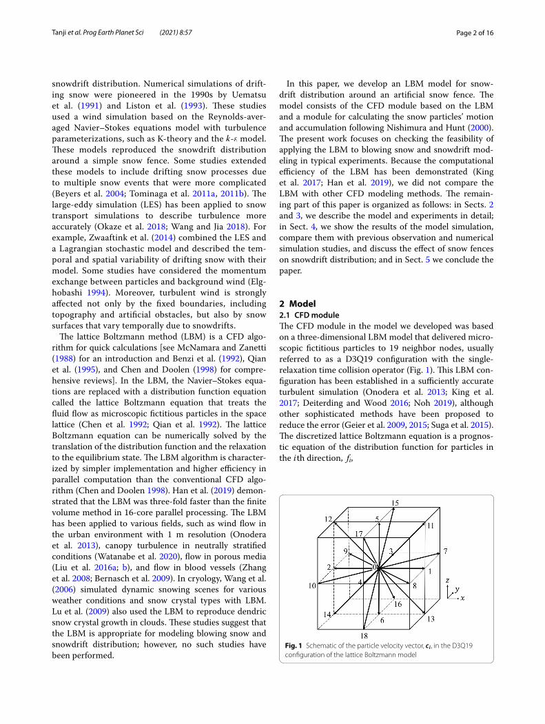
2 Model2.1 CFD moduleThe CFD module in the model we developed was based on a three-dimensional LBM model that delivered micro-scopic fictitious particles to 19 neighbor nodes, usually referred to as a D3Q19 configuration with the single-relaxation time collision operator (Fig. 1). This LBM con-figuration has been established in a sufficiently accurate turbulent simulation (Onodera et al. 2013; King et al. 2017; Deiterding and Wood 2016; Noh 2019), although other sophisticated methods have been proposed to reduce the error (Geier et al. 2009, 2015; Suga et al. 2015). The discretized lattice Boltzmann equation is a prognos-tic equation of the distribution function for particles in the i th direction, fi,
Fig. 1 Schematic of the particle velocity vector, ci , in the D3Q19 configuration of the lattice Boltzmann model

Page 3 of 16Tanji et al. Prog Earth Planet Sci (2021) 8:57
where r is the particle position vector, �t is the time increment, �i is the collision term, and ci is the particle velocity vector.
The Bhatnagar–Gross–Krook approximation reduced collision term �i to the relaxation to the equilibrium state of the distribution function (Chen et al. 1992; Qian et al. 1992),
Here, τ is the relaxation time as a function of viscosity ν∗,
where c is the discrete speed, defined as �x�t , with spatial
increment �x . ν∗ is defined as ν∗ = ν0n + νt , where ν0n is the non-dimensional viscosity of the air ( 4.0× 10⁻⁶ ) and νt is the eddy viscosity, given in Eq. (7). f̂i is the equilibrium distribution function for particles in the i th direction, cal-culated in the D3Q19 configuration as
where
the lattice speed of sound cs = 1/√3 , and ρ and u are the
macroscopic density and velocity, respectively, calculated in the D3Q19 configuration as
(1)fi(r + ci�t, t +�t) = fi(r, t)+�i�t,
(2)�i = −1
τ
(fi − f̂i
).
(3)τ =1
2+
3ν∗c2�t
(4)f̂i = wiρ⌈1+(ci • u)
c2s+
(ci • u)2
2c4s−
|u|2
2c2s⌉,
(5)wi =
13 (i = 0)
118 (i = 1, 2, . . . , 6)136 (i = 7, 8, . . . , 18)
,
The dimensional variables are transferred from the non-dimensional distribution function by multiplying the non-dimensional value by 50.0 to give the same Reynold numbers.
The sub-grid scale parameterization (Feng et al. 2007; Onodera et al. 2013; Wang et al. 2014; Suga et al. 2015) was implemented to estimate the eddy kinematic viscosity, νt . We used the Smagorinsky model (Smagorinsky 1963), in which νt is related to velocity gradient tensor S by
where Smagorinsky coefficient C = 0.12 (Tominaga et al. 2008; Okaze et al. 2021) and C = 60 in the damping zone, which consists of 15 grids from the outlet boundary to damp the numerical oscillation near the outlet (Inagaki et al. 2017). � is the cubic root of the local mesh volume. ∣∣S∣∣ was estimated in the D3Q19 configuration as
where cij and cik are the j th and k th components of ci , respectively.
The model domain was a finite channel in the three-dimensional space spanned by the wind direction, x , the horizontal direction normal to x (or fence direction), y , and the vertical direction, z . Hereafter, for convenience, the negative and positive ends of x in the domain are called the western and eastern boundaries, those of y are called the southern and northern boundaries, and those of z are called the bottom and top boundaries, respec-tively. The horizontal direction is rotationally invariant in this system.
The LBM represents the western boundary condi-tion with inflow u0(x, y, z) = (u0
(y, z
), v0
(y, z
),w0(y, z))
(Sect. 2.2) as
(6)ρ =18∑
i=0
fi, andu =1
ρ
18∑
i=0
fici.
(7)νt = C�2∣∣S∣∣,
(8)∣∣S∣∣ =
3
2ρτ
√√√√2
3∑
k=1
3∑
j=1
18∑
i=0
(fi − f̂i
)cijcik ,
(9)
f1 = f2 +ρu0
3,
f7 = f10 +f4 + f17 + f18 − f3 − f15 − f16
2+
ρ(u0 + v0)
6+
ρv0
3,
f8 = f9 +f3 + f15 + f16 − f4 − f17 − f18
2+
ρ(u0 − v0)
6−
ρv0
3,
f11 = f14 +f6 + f16 + f18 − f5 − f15 − f17
2+
ρ(u0 + w0)
6+
ρw0
3, and
f13 = f12 +f5 + f15 + f17 − f6 − f16 − f18
2+
ρ(u0 − w0)
6−
ρw0
3.
Page 4 of 16Tanji et al. Prog Earth Planet Sci (2021) 8:57
On the other side, the LBM represents the free-flow condition at the eastern boundary (Hecht and Harting 2010) as
where
The southern and northern boundaries are peri-odic. Distribution functions f3, f7 , f9 , f15 , and f16 at the southern boundary are equal to those at the northern
(10)
f2 = f1 −ue
3,
f10 = f7 −f4 + f17 + f18 − f3 − f15 − f16
4−
ue
6,
f9 = f8 −f3 + f15 + f16 − f4 − f17 − f18
4−
ue
6,
f14 = f11 −f6 + f16 + f18 − f5 − f15 − f17
4−
ue
6, and
f12 = f13 −f5 + f15 + f17 − f6 − f16 − f18
2−
ue
6,
(11)
ue =− 1+ f0 + f3 + f4 + f5 + f6 + f15 + f16
+ f17 + f18 + 2(f1 + f7 + f8 + f11 + f13
).
boundary; and distribution functions f4 , f8 , f10 , f17 , and f18 at the northern boundary are equal to those at the southern boundary. The top boundary was a free-slip boundary (i.e., dudz = 0 ). The LBM representation was
The bottom boundary was no-slip (i.e., u = 0 ), so that the LBM represented it as bounce-back,
The boundary on the fence was also no-slip as bounce-back and was written similarly to Eq. (13).
2.2 Inflow turbulence generationWe generated the artificial inflow turbulence and imposed it as the inflow on the western boundary. The inflow turbulence was generated as two-dimensional digital-filtered random data by controlling the time and spatial autocorrelations of the resultant inflow turbu-lence (Okaze and Mochida 2017; Xie and Castro 2008). The total inflow, u0(y, z, t) , from the western boundary was divided into the time average, 〈u0〉 , and the deviation from the time average, u′
0 . We assumed that the model domain was the constant flux layer. The wind direction of the time-averaged vector was only eastward, and the wind speed followed the logarithmic profile of
where u∗ is the friction velocity (a parameter to be given), z0 is the roughness length for flat snow surface (0.1 mm; Hiroo and Ishida 1973), and κ is von Karman’s constant (0.4). Using other common assumptions (Okaze and Mochida 2018), Reynolds stress tensor R for the inflow turbulence was parameterized as
The deviation from the time average was computed as u
′
0
(y, z, t
)=
∼R �(y, z, t) , where
∼R is the Cholesky decom-
position of R and � is the numerical solution of the sto-chastic equation (Xie and Castro 2008) of
(12)f6 = f5, f13 = f11, f14 = f12, f16 = f15, and f18 = f17.
(13)f5 = f6, f11 = f14, f12 = f13, f15 = f18, and f17 = f16.
(14)�u0(z)� =u∗κln
(z
z0
),
(15)
R =
�u′
0u′0� �u′
0v′0� �u′
0w′0�
�v′0u′0� �v′0v
′0� �v′0w
′0�
�w′0u
′0� �w′
0v′0� �w′
0w′0�
= u2∗
10/3 0 −10 5/3 0−1 0 5/3
.
(16)
�(y, z, t +�t
)= �
(y, z, t
)exp
(−�t
T
)
+ ψ(y, z, t +�t
){1− exp
(−2�t
T
)}1/2
,
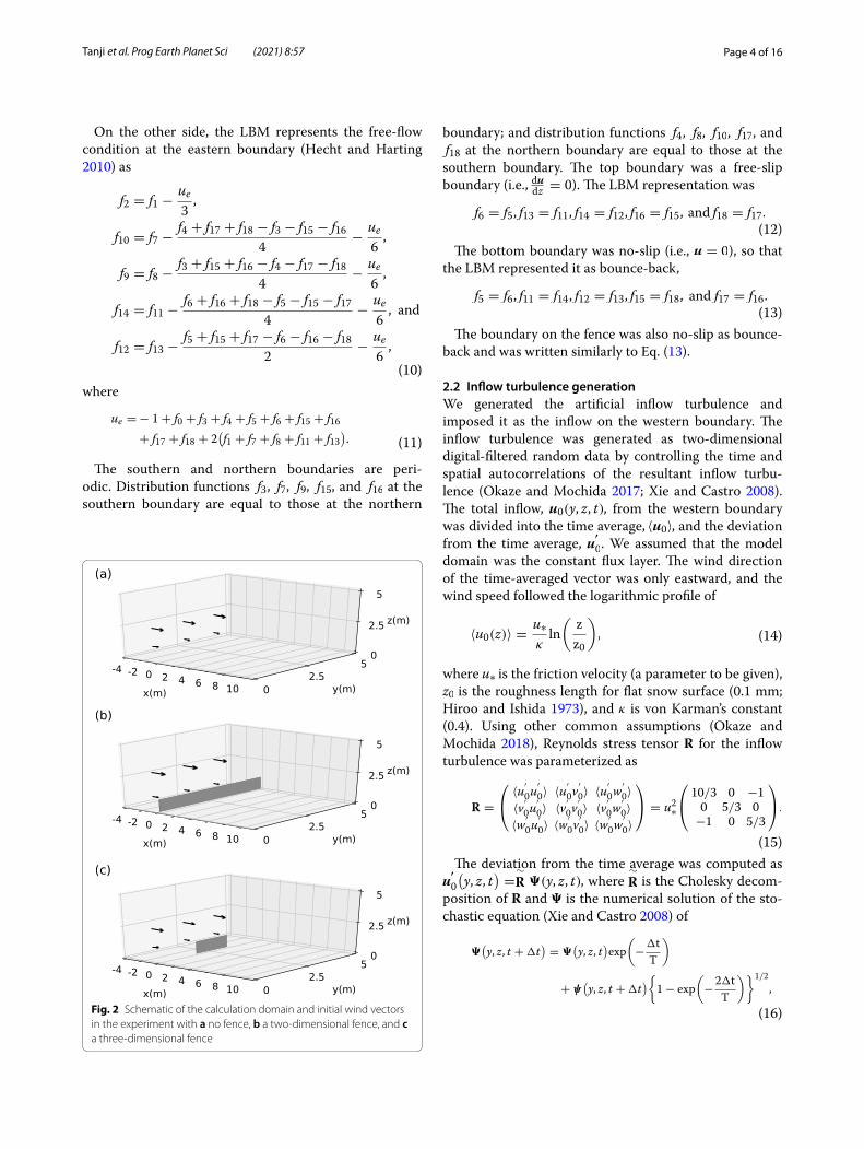
Fig. 2 Schematic of the calculation domain and initial wind vectors in the experiment with a no fence, b a two-dimensional fence, and c a three-dimensional fence

Page 5 of 16Tanji et al. Prog Earth Planet Sci (2021) 8:57
from the initial condition of �(y, z, 0
)= ψ
(y, z, 0
) . Here,
T is the characteristic timescale and ψ is the digital-filtered normal random numbers that satisfy a spatial autocorrelation with characteristic length L (Klein et al. 2003).ψ
(y, z, t
) was generated at each time step with a dif-
ferent random number. Following the modified Prandtl theory (Okuma et al. 1996), L was parameterized as
Then, by assuming Taylor’s hypothesis of frozen tur-bulence, characteristic timescale T was parameterized as
The inflow was numerically generated with the same grid spacing and the same time interval as the CFD module.
2.3 Snow particle moduleThe snow particle module in the model followed Nishimura and Hunt (2000) and Nemoto and Nishimura (2004). Assuming that drifting snow par-ticles were spherical, made of ice, electrically neutral, and not driven by the lift force, the equation of motion for the particles is written as
where up (m s−1) is the particle velocity vector, u (m s−1) is the wind vector, VR =
∣∣up − u∣∣, g is gravity (9.8 m s−2),
ρa and ρp are the densities of air (1.34 kg m−3) and the particle (910 kg m−3), respectively, and d is the particle diameter (100 µm ; Nishimura et al. 2014). Cd is the drag coefficient for the particle (White 1974), calculated as
where ν0 is the viscosity of the air ( 10−5 m2 s−1 ). The terminal fall velocity of a snow particle was estimated from the vertical component of Eqs. (19) and (20) as 0.30 m s−1.
Observation results indicated that accumulated snow particles jumped out of the snow surface when the
(17)L =1
3κz.
(18)T =1
3κz�u0(z)�.
(19)dup
dt= −
3
4
(ρa
ρpd
)CdVR
(up − u
)− gk ,
(20)Cd =24ν0
VRd+
6
1+ VRd/ν0+ 0.4,
friction velocity was high enough to lift them (Shao and Li 1999; Nemoto and Nishimura 2004). Based on this result, we assumed that a snow particle fell on the bottommost level and occupied the first grid-cell when the friction velocity on the snow surface was below the threshold. The friction velocity, u∗ (m s−1), on the snow surface was estimated with a wall function by a two-layer model in Werner and Wenglem (1991) as
where zb is the height of the bottommost grid just above the snow surface, A = 8.3 , and B = 1/7 . This is a differ-ent definition of the friction velocity from the inflow gen-eration. The wind velocity at the first grid point varied in time, and then the wall unit in the first grid point was also changed. This approach automatically considered the linear and power law distributions with an instan-taneous wall unit calculated with the wind speed in the first grid point. The threshold of the friction velocity, u∗t was computed following Bagnold (1941) and Clifton et al. (2006) as
We assumed that no snow particles accumulated when the friction velocity was larger than this threshold. The aerodynamic entrainment, rebound, splash, mass loss by sublimation and disruption, the drag force on the fluid, and coalescence of snow particles by the collision were all neglected.
3 ExperimentsWe performed three experiments: with no fence, with a two-dimensional fence, and with a three-dimensional fence of 1.5 m in width (Fig. 2). The fence was set 4 m from the western boundary and was centered in the channel. The fence was non-porous, solid, and the thick-ness was 0.1 m and the height was 1 m. The following model settings were independent of the presence of the fence. The channel size was 15.75 × 5 × 5 m, with the grid spacing at 0.05 m. The origin of the x-coordinate was 4 m from the western boundary, at the position of the fence. In the CFD calculation, the integration time was 30 s and the time interval was 1 ms; the results were sampled every 0.02 s from the initial time. In the generation of the inflow turbulence, the 40 s data was stored with an inter-val of 4 ms. The inflow turbulence was generated with the friction velocity, such that the time-averaged wind
(21)u∗ =
�2ν0|u(zb)|
zbfor |u(zb)| ≤ ν0
2zbA
21−B
�1−B2 A
1+B1−B
�ν0zb
�1+B+ 1+B
A
�ν0zb
�B|u(zb)|
� 11+B
, for |u(zb)| ≥ ν02zb
A2
1−B
(22)u∗t = 0.2
√ρp − ρa
ρagd ∼ 0.163m s
−1.
Page 6 of 16Tanji et al. Prog Earth Planet Sci (2021) 8:57
speed was 6 m s−1 westerly at 10 m aloft in the log profile and the initial wind profile over the calculation domain was imposed as the same value. We used 30 s data for the generated inflow turbulence after the spin-up as the western boundary condition after linear interpolation as every 1 ms.
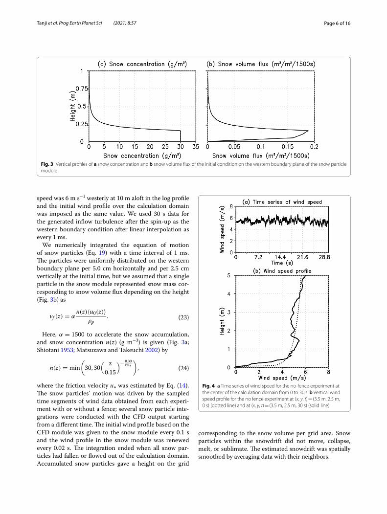
We numerically integrated the equation of motion of snow particles (Eq. 19) with a time interval of 1 ms. The particles were uniformly distributed on the western boundary plane per 5.0 cm horizontally and per 2.5 cm vertically at the initial time, but we assumed that a single particle in the snow module represented snow mass cor-responding to snow volume flux depending on the height (Fig. 3b) as
Here, α = 1500 to accelerate the snow accumulation, and snow concentration n(z) (g m−3) is given (Fig. 3a; Shiotani 1953; Matsuzawa and Takeuchi 2002) by
where the friction velocity u∗ was estimated by Eq. (14). The snow particles’ motion was driven by the sampled time segments of wind data obtained from each experi-ment with or without a fence; several snow particle inte-grations were conducted with the CFD output starting from a different time. The initial wind profile based on the CFD module was given to the snow module every 0.1 s and the wind profile in the snow module was renewed every 0.02 s. The integration ended when all snow par-ticles had fallen or flowed out of the calculation domain. Accumulated snow particles gave a height on the grid
(23)vf (z) = αn(z)�u0(z)�
ρp.
(24)n(z) = min
(30, 30
( z
0.15
)− 0.30κu∗
),
corresponding to the snow volume per grid area. Snow particles within the snowdrift did not move, collapse, melt, or sublimate. The estimated snowdrift was spatially smoothed by averaging data with their neighbors.
Fig. 3 Vertical profiles of a snow concentration and b snow volume flux of the initial condition on the western boundary plane of the snow particle module
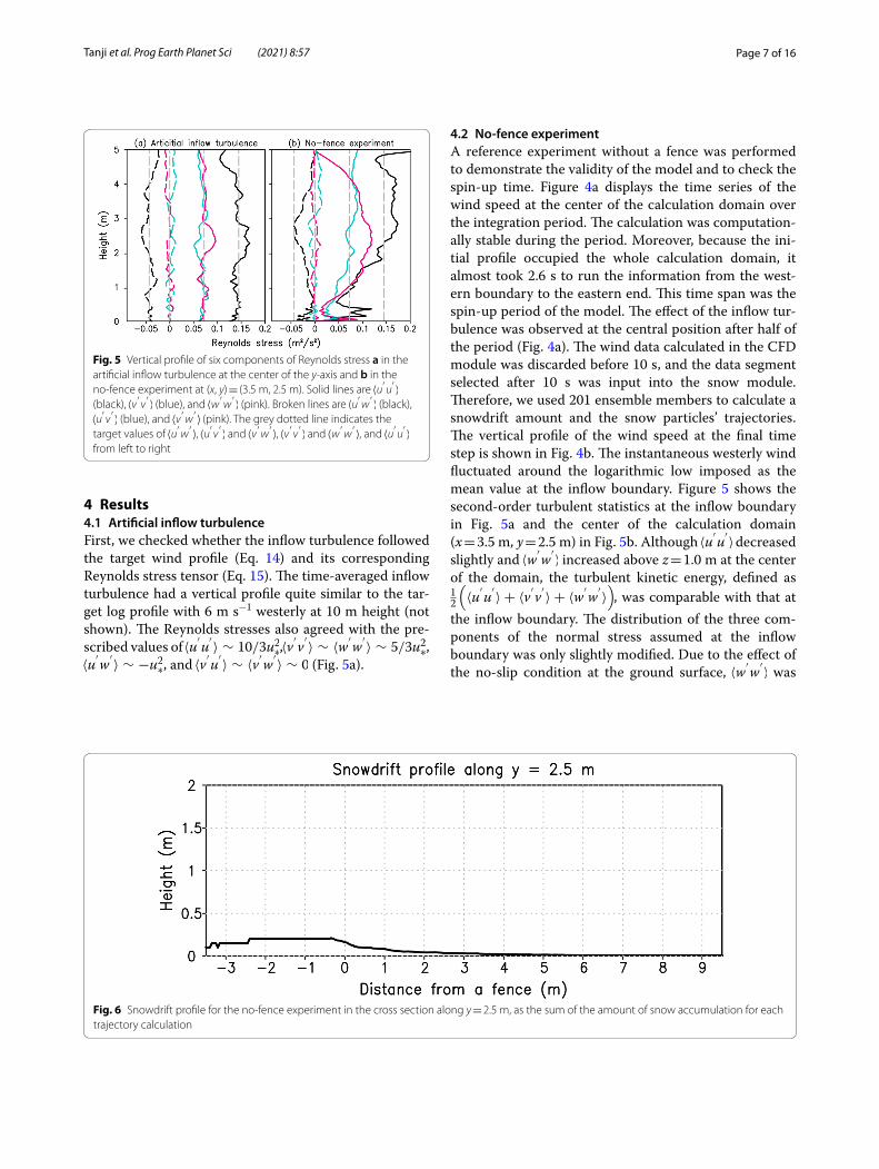
Fig. 4 a Time series of wind speed for the no-fence experiment at the center of the calculation domain from 0 to 30 s. b Vertical wind speed profile for the no fence experiment at (x, y, t) = (3.5 m, 2.5 m, 0 s) (dotted line) and at (x, y, t) = (3.5 m, 2.5 m, 30 s) (solid line)
Page 7 of 16Tanji et al. Prog Earth Planet Sci (2021) 8:57
4 Results4.1 Artificial inflow turbulenceFirst, we checked whether the inflow turbulence followed the target wind profile (Eq. 14) and its corresponding Reynolds stress tensor (Eq. 15). The time-averaged inflow turbulence had a vertical profile quite similar to the tar-get log profile with 6 m s−1 westerly at 10 m height (not shown). The Reynolds stresses also agreed with the pre-scribed values of �u′
u′ � ∼ 10/3u2∗,�v
′v′ � ∼ �w′
w′ � ∼ 5/3u2∗ ,
�u′w
′ � ∼ −u2∗ , and �v′u′ � ∼ �v′w′ � ∼ 0 (Fig. 5a).
4.2 No‑fence experimentA reference experiment without a fence was performed to demonstrate the validity of the model and to check the spin-up time. Figure 4a displays the time series of the wind speed at the center of the calculation domain over the integration period. The calculation was computation-ally stable during the period. Moreover, because the ini-tial profile occupied the whole calculation domain, it almost took 2.6 s to run the information from the west-ern boundary to the eastern end. This time span was the spin-up period of the model. The effect of the inflow tur-bulence was observed at the central position after half of the period (Fig. 4a). The wind data calculated in the CFD module was discarded before 10 s, and the data segment selected after 10 s was input into the snow module. Therefore, we used 201 ensemble members to calculate a snowdrift amount and the snow particles’ trajectories. The vertical profile of the wind speed at the final time step is shown in Fig. 4b. The instantaneous westerly wind fluctuated around the logarithmic low imposed as the mean value at the inflow boundary. Figure 5 shows the second-order turbulent statistics at the inflow boundary in Fig. 5a and the center of the calculation domain (x = 3.5 m, y = 2.5 m) in Fig. 5b. Although �u′
u′ � decreased
slightly and �w′w
′ � increased above z = 1.0 m at the center of the domain, the turbulent kinetic energy, defined as 12
(�u′
u′ � + �v′v′ � + �w′
w′ �) , was comparable with that at
the inflow boundary. The distribution of the three com-ponents of the normal stress assumed at the inflow boundary was only slightly modified. Due to the effect of the no-slip condition at the ground surface, �w′
w′ � was
Fig. 5 Vertical profile of six components of Reynolds stress a in the artificial inflow turbulence at the center of the y-axis and b in the no-fence experiment at (x, y) = (3.5 m, 2.5 m). Solid lines are �u′
u′ �
(black), �v ′v ′ � (blue), and �w ′w
′ � (pink). Broken lines are �u′w
′ � (black), �u′
v′ � (blue), and �v ′w ′ � (pink). The grey dotted line indicates the
target values of �u′w
′ � , �u′v′ � and �v ′w ′ � , �v ′v ′ � and �w ′
w′ � , and �u′
u′ �
from left to right
Fig. 6 Snowdrift profile for the no-fence experiment in the cross section along y = 2.5 m, as the sum of the amount of snow accumulation for each trajectory calculation

Page 8 of 16Tanji et al. Prog Earth Planet Sci (2021) 8:57
decreased near the surface, which could decrease �u′w
′ � , especially near the surface at the center of the domain. However, �u′
w′ � at the center was still half the prescribed
value at the inflow boundary.Figure 6 shows the snowdrift distribution as the sum
of the amount of snow accumulation in each trajectory calculation. According to Eqs. (19) and (24), the terminal fall velocity of snow particles was 0.3 m s−1, and snow particles below a height of 0.5 m at the initial position had a large volume flux. Snow particles were advected by the background flow of ~ 4 m s−1 until deposition. Hence, most of the snow particles fell within 7 m of the western boundary (Fig. 6). The horizontal distribution of the snowdrift depended on the vertical distribution of the snow volume flux. The height of the snowdrift was expected to be about 0.2 m in the calculation domain if the snow volume flux exceeded 6.0× 10⁻⁷ m3m−2 s−1 , corresponding to the flux at a height of 0.6 m. No more snow accumulation was possible after the friction veloc-ity exceeded the threshold (Eq. 22). The results indicated that we could test the blocking effect of a fence at x = 0 because a snowdrift was formed beyond the point with-out the fence.
4.3 Two‑dimensional fence experimentThe horizontal wind observed in the no-fence experi-ment was distorted by the two-dimensional fence nor-mal to the dominant wind direction, which created an ascending motion on the windward side and a swirling eddy in the cross section on the leeward side (two snap-shots in Fig. 7). The upper-level wind was intensified around the top of the fence. These wind profile features were consistent with previous studies (Uematsu et al. 1991; Liu et al. 2016a, b). However, the eddies were gen-erated successively from the leeward side of the fence and flowed downstream following the dominant wind flow, and the size and position of the eddies in the cross sec-tion varied irregularly over time (Fig. 7). At 10 s, a single eddy extended 1 m from the fence and there was another larger eddy from x = 6 to 8 m (Fig. 7a). The large eddy flowed in the eastern direction and left the domain after 11 s (not shown). At 26 s, there were large eddies just to the east of the fence and further downstream from x = 3 to 6 m (Fig. 7b). These larger eddies had a strong reverse flow near the surface because the intensified wind at the top of the fence was separated behind the fence. Eddies
Fig. 7 Snapshots of the wind vectors (vectors) and vorticity (shading) around the two-dimensional fence in the cross section along y = 2.5 m at a 10 and b 26 s. The solid line at x = 0 shows the two-dimensional fence

Page 9 of 16Tanji et al. Prog Earth Planet Sci (2021) 8:57
successively separated from the east side of the fence. The eddies caused by the fence augmented the fluctuations with a larger scale and a lager timescale.
The snowdrift distribution in the two-dimensional fence experiment (Fig. 8a) was different from that in the no-fence experiment (Fig. 6). Almost all of the snowdrift
Fig. 8 a Snowdrift profile around the two-dimensional fence in the cross section along y = 2.5 m, as the sum of the amount of snow accumulation of each trajectory calculation. b–d Ensemble trajectories of snow particles at the center of the y-axis around the two-dimensional fence driven by all the wind data segments. The initial heights of the particles are b 0.3, c 0.4, and d 1.4 m. The position of the fence is shown by a solid line
Page 10 of 16Tanji et al. Prog Earth Planet Sci (2021) 8:57
was distributed on the windward side of the fence because the surface wind speed was attenuated just to the west of the fence. The highest snowdrift was about 0.5 m high at x = −1.3m . These results were consistent with previous studies using a conventional numerical simula-tion (Uematsu et al. 1991; Alhajraf 2004) and observa-tions (Tabler 1994). On the leeward side of the fence, few snowdrifts formed except for from x = 5 to 7 m. This dis-tribution was consistent with the first snowdrift develop-ment regime in Tabler (1994), which is explained in detail in Sect. 5. There were three reasons for this result. First, most of the snow particles that went over the fence did not accumulate just east of the fence because the strong wind above the fence accelerated the snow particles. Fig-ure 8b–d show the trajectories of three initial positions of the snow particles driven by all the wind profile data seg-ments. Most of the particles starting from higher heights went over the fence and were blown through the calcu-lation domain, such as the particles that started from a height of 1.4 m (Fig. 8d). However, most of the particles starting from a height of 0.3 m did not get over the fence (Fig. 8b) because these particles reached the grid on the windward side of the fence that had a friction veloc-ity below the threshold (Eq. 22). Second, the eddies that were successively generated on the leeward side of the
fence disturbed the snowdrift development at a certain point because these transient eddies were generated by inflow turbulence and the snow accumulation in a single trajectory calculation depended on the transient eddies. For example, some particles starting from a height of 0.4 m subsequently followed the streamlines of the swirl-ing eddies and fell to the east of the fence (Fig. 8c), but these particles fell on different grids in each wind profile data segment. Third, most of the snow particles accumu-lating on the leeward side of the fence had a small snow volume flux, such as the particles starting from a height of 1.4 m. The snowdrift at the point where these parti-cles fell was less than 5 cm high (Fig. 8a) because these particles had a small snow volume flux. In contrast, most of the snow particles starting at a height of 0.3 m with a large snow volume flux fell on the surface of the wind-ward side. Thus, the two-dimensional snow fence was an effective obstacle to snowdrift development on the lee-ward side compared with the snowdrift distribution in the no-fence experiment (Fig. 6).
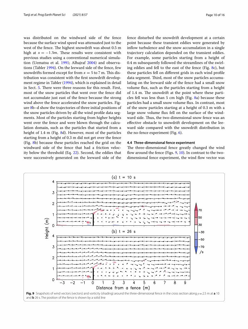
4.4 Three‑dimensional fence experimentThe three-dimensional fence greatly changed the wind flow around the fence (Figs. 9, 10). In contrast to the two-dimensional fence experiment, the wind flow vector was
Fig. 9 Snapshots of wind vectors (vectors) and vorticity (shading) around the three-dimensional fence in the cross section along y = 2.5 m at a 10 and b 26 s. The position of the fence is shown by a solid line

Page 11 of 16Tanji et al. Prog Earth Planet Sci (2021) 8:57
Fig. 10 Snapshots of wind vectors (vectors) and vorticity (shading) around the three-dimensional fence on the horizontal plane along z = 0.5 m at a 10 and b 26 s. The position of the fence is shown by a solid line
Fig. 11 a Snowdrift height around the three-dimensional fence in the cross section along b y = 2.5 m and c x = 2.5 m. The snowdrift is the sum of the amount of snow accumulation of each trajectory calculation. The position of the fence is shown by a solid line in a and b

Page 12 of 16Tanji et al. Prog Earth Planet Sci (2021) 8:57
three-dimensional in the three-dimensional fence experi-ment. The reverse flow along the center of the fence was weaker than that in the two-dimensional fence experi-ment around the surface on the leeward side around x = 2 m at 10 s (Fig. 9a). The low-level wind flow was horizontally diffluent and went round the fence, and there was a dipole pattern on the leeward side, with a weak wake flow toward the center of the fence on the horizontal plane at z = 0.5 m (Fig. 10a). The wind flow at 26 s had a weak eddy from x = 1 to 3m on the verti-cal plane (Fig. 9b). These features were consistent with a previous study that simulated wind flow around a three-dimensional obstacle with the LBM (Han et al. 2021). On the horizontal plane, there was still a dipole pattern, but the turbulent flow 4 m east of the fence was more intense after a while due to the spread of turbulence generated by eddies on the horizontal plane on the leeward side (Fig. 10b).
In the three-dimensional fence experiment, the snow-drift had a two-dimensional distribution (Fig. 11a). The snowdrift along the center of the y-axis on the windward side was similar to that in the two-dimensional fence
experiment (Fig. 11b). On the leeward side, snowdrift was not formed behind the fence along the center of the y-axis, but it was formed in the no-fence zone (Fig. 11c). This snowdrift developed ahead of the split flow because there were weak flow lines around the surface (Fig. 10). This snowdrift profile associated with the split flow was consistent with previous studies of snowdrifts around cubes (Beyers et al. 2004; Okaze et al. 2013). The snow particles clarified the three-dimensional trajectories for snow deposition. All of the particles starting from heights of 0.3 (not shown) and 0.4 m (Fig. 12a) fell on the wind-ward side of the fence, whereas some particles from the same heights went over the fence in the two-dimensional fence experiment. This difference was probably caused by the lower wind speed just above the three-dimensional fence due to the energy loss accompanied by the horizon-tal diffluent flow (Fig. 10). The snow particles’ trajectories on a horizontal plane indicated the snowdrift formation process along the split streaks on the leeward side. For example, some snow particles from (y, z) = (2.5 m, 0.5 m) did not flow over the fence because they collided with the fence, whereas most of the snow particles from (y, z) = (1.5 m, 0.5 m) did not collide with the fence and fell along the stream of the horizontal diffluent flow (Fig. 12c, d). These low-level particles formed the forking snowdrift on the leeward side.
Fig. 12 Ensemble trajectories of snow particles at a, b the center of the y-axis and c, d along z = 0.5 m around the three-dimensional fence driven by all the wind data segments. The initial positions of the particles are (y, z) = a (2.5 m, 0.4 m), b (2.5 m, 1.4 m), c (1.5 m, 0.5 m), and d (2.5 m, 0.5 m). The position of the fence is shown by a solid line
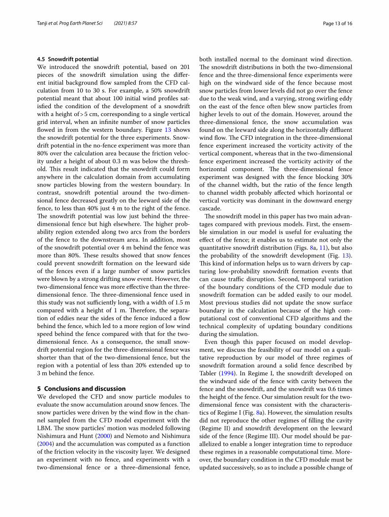
Fig. 13 Snowdrift potential a for no fence, b around the two-dimensional fence, and c around the three-dimensional fence. The position of the fence is shown by a solid line
Page 13 of 16Tanji et al. Prog Earth Planet Sci (2021) 8:57
4.5 Snowdrift potentialWe introduced the snowdrift potential, based on 201 pieces of the snowdrift simulation using the differ-ent initial background flow sampled from the CFD cal-culation from 10 to 30 s. For example, a 50% snowdrift potential meant that about 100 initial wind profiles sat-isfied the condition of the development of a snowdrift with a height of > 5 cm, corresponding to a single vertical grid interval, when an infinite number of snow particles flowed in from the western boundary. Figure 13 shows the snowdrift potential for the three experiments. Snow-drift potential in the no-fence experiment was more than 80% over the calculation area because the friction veloc-ity under a height of about 0.3 m was below the thresh-old. This result indicated that the snowdrift could form anywhere in the calculation domain from accumulating snow particles blowing from the western boundary. In contrast, snowdrift potential around the two-dimen-sional fence decreased greatly on the leeward side of the fence, to less than 40% just 4 m to the right of the fence. The snowdrift potential was low just behind the three-dimensional fence but high elsewhere. The higher prob-ability region extended along two arcs from the borders of the fence to the downstream area. In addition, most of the snowdrift potential over 4 m behind the fence was more than 80%. These results showed that snow fences could prevent snowdrift formation on the leeward side of the fences even if a large number of snow particles were blown by a strong drifting snow event. However, the two-dimensional fence was more effective than the three-dimensional fence. The three-dimensional fence used in this study was not sufficiently long, with a width of 1.5 m compared with a height of 1 m. Therefore, the separa-tion of eddies near the sides of the fence induced a flow behind the fence, which led to a more region of low wind speed behind the fence compared with that for the two-dimensional fence. As a consequence, the small snow-drift potential region for the three-dimensional fence was shorter than that of the two-dimensional fence, but the region with a potential of less than 20% extended up to 3 m behind the fence.
5 Conclusions and discussionWe developed the CFD and snow particle modules to evaluate the snow accumulation around snow fences. The snow particles were driven by the wind flow in the chan-nel sampled from the CFD model experiment with the LBM. The snow particles’ motion was modeled following Nishimura and Hunt (2000) and Nemoto and Nishimura (2004) and the accumulation was computed as a function of the friction velocity in the viscosity layer. We designed an experiment with no fence, and experiments with a two-dimensional fence or a three-dimensional fence,
both installed normal to the dominant wind direction. The snowdrift distributions in both the two-dimensional fence and the three-dimensional fence experiments were high on the windward side of the fence because most snow particles from lower levels did not go over the fence due to the weak wind, and a varying, strong swirling eddy on the east of the fence often blew snow particles from higher levels to out of the domain. However, around the three-dimensional fence, the snow accumulation was found on the leeward side along the horizontally diffluent wind flow. The CFD integration in the three-dimensional fence experiment increased the vorticity activity of the vertical component, whereas that in the two-dimensional fence experiment increased the vorticity activity of the horizontal component. The three-dimensional fence experiment was designed with the fence blocking 30% of the channel width, but the ratio of the fence length to channel width probably affected which horizontal or vertical vorticity was dominant in the downward energy cascade.
The snowdrift model in this paper has two main advan-tages compared with previous models. First, the ensem-ble simulation in our model is useful for evaluating the effect of the fence; it enables us to estimate not only the quantitative snowdrift distribution (Figs. 8a, 11), but also the probability of the snowdrift development (Fig. 13). This kind of information helps us to warn drivers by cap-turing low-probability snowdrift formation events that can cause traffic disruption. Second, temporal variation of the boundary conditions of the CFD module due to snowdrift formation can be added easily to our model. Most previous studies did not update the snow surface boundary in the calculation because of the high com-putational cost of conventional CFD algorithms and the technical complexity of updating boundary conditions during the simulation.
Even though this paper focused on model develop-ment, we discuss the feasibility of our model on a quali-tative reproduction by our model of three regimes of snowdrift formation around a solid fence described by Tabler (1994). In Regime I, the snowdrift developed on the windward side of the fence with cavity between the fence and the snowdrift, and the snowdrift was 0.6 times the height of the fence. Our simulation result for the two-dimensional fence was consistent with the characteris-tics of Regime I (Fig. 8a). However, the simulation results did not reproduce the other regimes of filling the cavity (Regime II) and snowdrift development on the leeward side of the fence (Regime III). Our model should be par-allelized to enable a longer integration time to reproduce these regimes in a reasonable computational time. More-over, the boundary condition in the CFD module must be updated successively, so as to include a possible change of
Page 14 of 16Tanji et al. Prog Earth Planet Sci (2021) 8:57
flow due to a change in snowdrift surface. Furthermore, the resuspension and redeposition of the particles should be included in the snow particle module to estimate snowdrifts more accurately.
To achieve a more accurate snowdrift simulation, other snow motion and accumulation processes must be included. For example, resuspension of snow particles from the surface is an important process in drifting snow. In the present model, this process was implicitly included in the prohibition of snow accumulation on the surface by strong wind. However, we did not consider the trajec-tories and redeposition of resuspended snow particles. The resuspension processes are aerodynamic entrain-ment, rebound and splash (Shao and Li 1999; Ammi et al. 2009). Moreover, the initial condition of the snow surface should be prescribed because snow particles on the sur-face drift when the friction velocity exceeds the threshold velocity.
This paper was limited to experiments with no inter-actions between snow and wind. In this study, snow particles were affected by the wind, but the wind was not affected by the snow particles; thus, the coupling was one-way. By considering the interaction between snow and wind as a two-way coupling, the wind veloc-ity is slightly reduced by the momentum exchange between snow particles and wind. This modification may change the trajectory of snow particles (Figs. 8b–d, 12) so that they fall short on the windward side of the fence. Moreover, there is an interaction between the snow surface and wind flow. The snow accumula-tion changes the bottom boundary condition in the CFD calculation. Our model can be extended easily to allow temporal variation of the boundary conditions because the LBM is simpler than other algorithms and more suitable for complicated boundary conditions. Because the snow particles generally accumulated where the wind speed was low on the windward side
of the three-dimensional fence (Fig. 11), we can easily presume that the snow surface on the windward side is asymptotic to a streamline that crosses the top of the fence. We can readily implement this interaction pro-cess simply by combining the CFD and the snow parti-cle modules, but this will be addressed in future work.
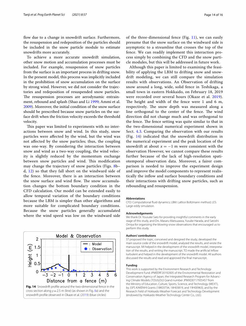
Although this paper is limited to examining the feasi-bility of applying the LBM to drifting snow and snow-drift modeling, we can still compare the simulation results with observations. An Observation of drifting snow around a long, wide, solid fence in Teshikaga, a small town in eastern Hokkaido, on February 18, 2019 were recorded over several hours (Okaze et al. 2019). The height and width of the fence were 1 and 6 m, respectively. The snow depth was measured along a line orthogonal to the center of the fence. The wind direction did not change much and was orthogonal to the fence. The fence setting was quite similar to that in the two-dimensional numerical experiment shown in Sect. 4.3. Comparing the observation with our results (Fig. 14) indicated that the snowdrift distribution in the numerical experiment and the peak location of the snowdrift at about x = −1 m were consistent with the observation However, we cannot compare these results further because of the lack of high-resolution spati-otemporal observation data. Moreover, a fairer com-parison is needed to improve the experiment design and improve the model components to represent realis-tically the inflow and surface boundary conditions and their interactions with drifting snow particles, such as rebounding and resuspension.
AbbreviationsCFD: Computational fluid dynamics; LBM: Lattice Boltzmann method; LES: Large-eddy simulation.
AcknowledgementsWe thank Dr. Yousuke Sato for providing insightful comments in the early stage of this study, and Drs. Masaru Matsuzawa, Yusuke Harada, and Satoshi Omiya for organizing the blowing-snow observations that encouraged us to perform this study.
Authors’ contributionsST proposed the topic, conceived and designed the study, developed the main source code of the snowdrift model, analyzed the results, and wrote the manuscript. MI helped in the development of the snowdrift model, interpreta-tion of the results, and writing the manuscript. TO made the artificial inflow turbulent and helped in the development of the snowdrift model. All authors discussed the results and read and approved the final manuscript.
FundingThis work is supported by the Environment Research and Technology Development Fund JPMEERF20192005 of the Environmental Restoration and Conservation Agency of Japan, the Integrated Research Program for Advanc-ing Climate Models (TOUGOU) Grand number JPMXD0717935457 from the Ministry of Education, Culture, Sports, Science, and Technology (MEXT), by JSPS KAKENHI Grants (18K03734, 18H03819, and 19H00963), and by the Research Field of Hokkaido Weather Forecast and Technology Development (endowed by Hokkaido Weather Technology Center Co., Ltd.).
Fig. 14 Snowdrift profile around the two-dimensional fence in the cross section along y = 2.5 m (line) (as shown in Fig. 8a) and the snowdrift profile observed in Okaze et al. (2019) (blue circles)

Page 15 of 16Tanji et al. Prog Earth Planet Sci (2021) 8:57
Availability of data and materialsThe datasets used during the current study are available from the correspond-ing author on reasonable request.
Declarations
Competing interestsThe authors declare that they have no competing interests.
Author details1 Graduate School of Science, Hokkaido University, N10W8, Sapporo 0600810, Japan. 2 Faculty of Science, Hokkaido University, N10W8, Sapporo 0600810, Japan. 3 Center for Natural Hazards Research, Hokkaido University, N9W9, Sapporo 0608589, Japan. 4 School of Environment and Society, Tokyo Institute of Technology, 4259 Nagatsuta-cho, Midori-ku, Yokohama 2268502, Japan.
Received: 19 March 2021 Accepted: 27 September 2021
ReferencesAlhajraf S (2004) Computational fluid dynamic modeling of drifting particles at
porous fences. Environ Model Softw 19:163–170. https:// doi. org/ 10. 1016/ S1364- 8152(03) 00118-X
Ammi M, Oger L, Beladjine D, Valance A (2009) Three-dimensional analysis of the collision process of a bead on a granular packing. Phys Rev E 79:021305. https:// doi. org/ 10. 1103/ PhysR evE. 79. 021305
Bagnold RA (1941) The physics of blown sand and desert dunes. Methuen, London
Benzi R, Succi S, Vergassola M (1992) The Lattice Boltzmann equation: theory and applications. Phys Rep 222:145–197. https:// doi. org/ 10. 1016/ 0370- 1573(92) 90090-M
Bernasch M, Fatica M, Melchionna S, Succi S, Kaxiras E (2009) A flexible high-performance lattice Boltzmann GPU code for the simulations of fluid flows in complex geometries. Concurr Comput Pract Exp 22:1–14. https:// doi. org/ 10. 1002/ cpe. 1466
Beyers JHM, Sundsbo PA, Harms TM (2004) Numerical simulation of three-dimensional, transient snow drifting around a cube. J Wind Eng Ind Aerodyn 92:725–747. https:// doi. org/ 10. 1016/j. jweia. 2004. 03. 011
Chen S, Doolen GD (1998) Lattice Boltzmann method for fluid flows. Annu Rev Fluid Mech 30:329–364. https:// doi. org/ 10. 1146/ annur ev. fluid. 30.1. 329
Chen H, Chen S, Matthaeus WH (1992) Recovery of the Navier Stokes equa-tions using a lattice-gas Boltzmann method. Phys Rev A 45:5339–5342. https:// doi. org/ 10. 1103/ PhysR evA. 45. R5339
Clifton A, Rüedi JD, Lehning M (2006) Snow saltation threshold measurements in a drifting snow wind tunnel. J Glaciol 39:585–596. https:// doi. org/ 10. 3189/ 17275 65067 81828 430
Deiterding R, Wood SL (2016) Predictive wind turbine simulation with an adap-tive lattice Boltzmann method for moving boundaries. J Phys Conf Ser 753:082005. https:// doi. org/ 10. 1088/ 1742- 6596/ 753/8/ 082005
Delpech P, Palier P, Gandemer J (1998) Snowdrifting simulation around Antarc-tic buildings. J Wind Eng Ind Aerodyn 74–76:567–576. https:// doi. org/ 10. 1016/ S0167- 6105(98) 00051-8
Elghobashi S (1994) On predicting particle-laden turbulent flows. Appl Sci Res 52:309–329. https:// doi. org/ 10. 1007/ BF009 36835
Feng YT, Han K, Owen DRJ (2007) Coupled lattice Boltzmann method and discrete element modelling of particle transport in turbulent fluid flows: computational issues. Int J Numer Methods Eng 72:1111–1134. https:// doi. org/ 10. 1002/ nme. 2114
Geier M, Greiner A, Korvink JG (2009) A factorized central moment lattice Boltzmann method. Eur Phys J Spec Top 171(1):55–61. https:// doi. org/ 10. 1140/ epjst/ e2009- 01011-1
Geier M, Schönherr M, Pasquali A, Krafczyk M (2015) The cumulant lattice Boltzmann equation in three dimensions: theory and validation. Comput Math Appl 70(4):507–547. https:// doi. org/ 10. 1016/j. camwa. 2015. 05. 001
Han M, Ooka R, Kikumoto H (2019) Lattice Boltzmann method-based large-eddy simulation of indoor isothermal airflow. Int J Heat Mass Transf 130:700–709. https:// doi. org/ 10. 1016/j. ijhea tmass trans fer. 2018. 10. 137
Han M, Ooka R, Kikumoto H (2021) Effects of wall function model in lattice Boltzmann method-based large-eddy simulation on built environment flows. Build Environ 195:107764. https:// doi. org/ 10. 1016/j. build env. 2021. 107764
Hecht M, Harting J (2010) Implementation of on-site velocity boundary condi-tions for D3Q19 lattice Boltzmann simulations. J Stat Mech. https:// doi. org/ 10. 1088/ 1742- 5468/ 2010/ 01/ P01018
Hiroo F, Ishida T (1973) Rate of Turbulent energy dissipation during snow drift-ing. Low Temp Sci Ser A Phys Sci 31:69–85
Inagaki A, Kanda M, Ahmad HN, Yagi A, Onodera N, Aoki T (2017) A numerical study of turbulence statistics and the structure of a spatially-developing boundary layer over a realistic urban geometry. Bound Layer Meteor 164:1651–2181. https:// doi. org/ 10. 1007/ s10546- 017- 0249-y
Kaneko M, Matsuzawa M, Watanabe T (2011) Experiments on snowdrift devel-opment and vehicle starting limit. Technical research presentation 2011 (in Japanese)
King MF, Khan A, Delbosc N, Gough HL, Halios C, Barlow JF, Noakes CJ (2017) Modelling urban airflow and natural ventilation using a GPU-based lattice-Boltzmann method. Build Environ 125:273–284. https:// doi. org/ 10. 1016/j. build env. 2017. 08. 048
Klein M, Sadiki A, Janicka J (2003) A digital filter based generation of inflow data for spatially developing direct numerical or large eddy simulations. J Comput Phys 186:652–665. https:// doi. org/ 10. 1016/ S0021- 9991(03) 00090-1
Lehning M, Volksch I, Gustafsson D, Nguyen TA, Stahli M, Zappa M (2006) ALPINE3D: a detailed model of mountain surface processes and its application to snow hydrology. Hydrol Proc 20:2111–2128. https:// doi. org/ 10. 1002/ hyp. 6204
Lehning M, Löwe H, Ryser M, Raderschall N (2008) Inhomogeneous precipita-tion distribution and snow transport in steep terrain. Water Resour Res 44:W07404. https:// doi. org/ 10. 1029/ 2007W R0065 45
Liston GE, Brown RL, Dent JD (1993) A two-dimensional computational model of turbulent atmospheric surface flows with drifting snow. Ann Glaciol 18:281–286. https:// doi. org/ 10. 3189/ S0260 30550 00116 54
Liu D, Li Y, Wang B, Hu P, Zhang J (2016a) Mechanism and effects of snow accumulations and controls by lightweight snow fences. J Mod Transp 24:261–269. https:// doi. org/ 10. 1007/ s40534- 016- 0115-5
Liu H, Kang Q, Leonardi CR, Schmieschek S, Narváez A, Jones BD, Williams JR, Valocchi AJ, Harting J (2016b) Multiphase lattice Boltzmann simulations for porous media applications. Comput Geosci 20:777–805. https:// doi. org/ 10. 1007/ s10596- 015- 9542-3
Lu GP, DePaolo DJ, Kang QJ, Zhang DX (2009) Lattice Boltzmann simulation of snow crystal growth in clouds. J Geophys Res 114:D07305. https:// doi. org/ 10. 1029/ 2008J D0110 87
Matsuzawa M, Takeuchi M (2002) A study of methods to estimate visibility based on weather conditions. Seppyo 64:77–85 (in Japanese)
McNamara GR, Zanetti G (1988) Use of the Boltzmann equation to simulate lattice-gas automata. Phys Rev Lett 61:2332–2335. https:// doi. org/ 10. 1103/ PhysR evLett. 61. 2332
Mott R, Schirmer M, Bavay M, Grünewald T, Lehning M (2010) Understanding snow-transport processes shaping the mountain snow-cover. Cryosphere 4:545–559. https:// doi. org/ 10. 5194/ tc-4- 545- 2010
Nemoto M, Nishimura K (2004) Numerical simulation of snow saltation and suspension in a turbulent boundary layer. J Geophys Res 109:D18206. https:// doi. org/ 10. 1029/ 2004J D0046 57
Nishimura K, Hunt JCR (2000) Saltation and incipient suspension above a flat particle bed below a turbulent boundary layer. J Fluid Mech 417:77–102. https:// doi. org/ 10. 1017/ S0022 11200 00010 14
Nishimura K, Yokoyama C, Ito Y, Nemoto M, Naaim-Bouvet F, Bellot H, Fujita K (2014) Snow particle speeds in drifting snow. J Geophys Res 119:9901–9913. https:// doi. org/ 10. 1002/ 2014J D0216 86
Noh HM (2019) Numerical analysis of aerodynamic noise from pantograph in high-speed trains using lattice Boltzmann method. Adv Mech Eng 11(7):1–12. https:// doi. org/ 10. 1177/ 16878 14019 863995
Okaze T, Mochida A (2017) Cholesky decomposition–based generation of artificial inflow turbulence including scalar fluctuation. Comput Fluids 159:23–32. https:// doi. org/ 10. 1016/j. compfl uid. 2017. 09. 005
Okaze T, Mochida A, Tominaga Y, Nemoto M, Sato T, Sasaki Y, Ichinohe K (2012) Wind tunnel investigation of drifting snow development in a bound-ary layer. J Wind Eng Ind Aerodyn 104–106:532–539. https:// doi. org/ 10. 1016/j. jweia. 2012. 04. 002

Page 16 of 16Tanji et al. Prog Earth Planet Sci (2021) 8:57
Okaze T, Tominaga Y, Mochida A (2013) Development of new snowdrift model based on two transport equations of drifting snow density, numerical prediction of snowdrift around buildings using CFD (part 2). J Environ Eng AIJ 78:149–156 (in Japanese)
Okaze T, Niiya H, Nishimura K (2018) Development of a large-eddy simulation coupled with Lagrangian snow transport model. J Wind Eng Ind Aerodyn 183:35–43. https:// doi. org/ 10. 1016/j. jweia. 2018. 09. 027
Okaze T, Kikumoto H, Ono H, Imano M, Ikegaya N, Hasama T, Nakao K, Kishida T, Tabata Y, Nakajima K, Yoshie R, Tominaga Y (2021) Large-eddy simula-tion of flow around an isolated building: a step-by-step analysis of influencing factors on turbulent statistics. Build Environ. https:// doi. org/ 10. 1016/j. build env. 2021. 108021
Okaze T, Mochida A (2018) Generation of artificial Inflow turbulence with digi-tal filter method for LES within built-up environment. In: 25th Symposium of wind engineering, pp 211–216 (in Japanese)
Okaze T, Niiya H, Omiya S, Sunako S, Nishimura K (2019) Observation of snow-drift around two-dimensional fence during a drifting snow event. In: JSSI and JSSE joint conference 2019 in Yamagata, p 110 (in Japanese)
Okuma T, Kanda J, Tamura Y (1996) Windproof design of buildings. Kajima Syuppan-kai (in Japanese)
Onodera N, Aoki T, Shimokawabe T, Kobayashi H (2013) A large-scale LES wind simulation using lattice Boltzmann method for a 10 km × 10 km area in Tokyo. In: High performance computing symposium, pp 123–131 (in Japanese)
Qian Y, d’Humieres D, Lallemand P (1992) Lattice BGK models for Navier-Stokes equation. Europhys Lett 17:479–484. https:// doi. org/ 10. 1209/ 0295- 5075/ 17/6/ 001
Qian YH, Succi S, Orszag SA (1995) Recent advances in lattice Boltzmann computing. Annu Rev Comput Phys 3:195–242. https:// doi. org/ 10. 1142/ 97898 12830 647_ 0006
Shao Y, Li A (1999) Numerical modelling of saltation in the atmospheric sur-face layer. Bound Layer Meteorol 91:199–225. https:// doi. org/ 10. 1023/A: 10018 16013 475
Shiotani M (1953) Note on the vertical distribution of density of blowing snow in the snow storm. Seppyo 15:6–9 (in Japanese)
Smagorinsky J (1963) General circulation experiments with the primitive equa-tions. I. The basic experiment. Mon Weather Rev 91:99–164. https:// doi. org/ 10. 1175/ 1520- 0493(1963) 091% 3c0099: GCEWTP% 3e2.3. CO;2
Suga K, Kuwata Y, Takashima K, Chikasue R (2015) A D3Q27 multiple-relaxa-tion-time lattice Boltzmann method for turbulent flows. Comput Math Appl 69:518–529. https:// doi. org/ 10. 1016/j. camwa. 2015. 01. 010
Tabler RD (1980) Geometry and density of drifts formed by snow fences. J Glaciol 26:405–419. https:// doi. org/ 10. 3189/ S0022 14300 00109 35
Tabler RD (1986) Snow fence handbook (Release 1.0). Tabler and Associates, Laramie, Wyoming
Tabler RD (1994) Design guidelines for the control of blowing and drifting snow. Strategic highway research program report SHRP-H-381
Takeuchi M (1980) Vertical profile and horizontal increase of drift-snow trans-port. J Glaciol 26:481–492. https:// doi. org/ 10. 3189/ S0022 14300 00109 96
Takeuchi M, Ishimoto K, Nohara T, Fukuzawa Y (1986) Dynamic threshold wind speed for suspension. In: Proceedings of the annual meeting of the Japanese Society of Snow and Ice (in Japanese)
Tominaga Y, Mochida A, Murakami S, Sawaki S (2008) Comparison of various revised k–ε models and LES applied to flow around a high-rise building
model with 1:1:2 shape placed within the surface boundary layer. J Wind Eng Ind Aerodyn 96:389–411. https:// doi. org/ 10. 1016/j. jweia. 2008. 01. 004
Tominaga Y, Mochida A, Okaze T, Sato T, Nemoto M, Motoyoshi H, Nakai S, Tsut-sumi T, Otsuki M, Uamatsu T, Yoshino H (2011a) Development of a system for predicting snow distribution in built-up environments: combining a mesoscale meteorological model and a CFD model. J Wind Eng Ind Aerodyn 99:460–468. https:// doi. org/ 10. 1016/j. jweia. 2010. 12. 004
Tominaga Y, Okaze T, Mochida A (2011b) CFD modeling of snowdrift around abuilding: an overview of models and evaluation of a new approach. Build Environ 46:899–910. https:// doi. org/ 10. 1016/j. build env. 2010. 10. 020
Uematsu T, Nakata T, Takeuchi K, Arisawa Y, Kaneda Y (1991) Three-dimensional numerical simulation of snowdrift. Cold Reg Sci Technol 20:65–73. https:// doi. org/ 10. 1016/ 0165- 232X(91) 90057-N
Vionnet V, Martin E, Masson V, Lac C, Bouvet F, Guyomarc’h G (2017) High-resolution large eddy simulation of snow accumulation in Alpine terrain. J Geophys Res 122:11005–11021. https:// doi. org/ 10. 1002/ 2017J D0269 47
Wang Z, Jia S (2018) A simulation of a large-scale drifting snowstorm in the turbulent boundary layer. Cryosphere 12:3841–3851. https:// doi. org/ 10. 5194/ tc- 12- 3841- 2018
Wang CB, Wang ZY, Xia T, Peng QS (2006) Real-time snowing simulation. Vis Comput 22:315–323. https:// doi. org/ 10. 1007/ s00371- 006- 0012-8
Wang X, Shangguan YQ, Onodera N, Kobayashi H, Aoki T (2014) Direct numeri-cal simulation and large eddy simulation on a turbulent wall-bounded flow using Lattice Boltzmann Method and multiple GPUs. Math Probl Eng. https:// doi. org/ 10. 1155/ 2014/ 742432
Watanabe T, Shimoyama K, Kawashima M, Mizoguchi Y, Inagaki A (2020) Large-eddy simulation of neutrally-stratified turbulent flow within and above plant canopy using the central-moments-based lattice Boltzmann method. Bound Layer Meteorol 176:35–60. https:// doi. org/ 10. 1007/ s10546- 020- 00519-8
Werner H, Wenglem H (1991) Large-eddy simulation of turbulent flow over and around a cube in a plate channel. In: Proceedings of 8th symposium on turbulent shear flows, pp 155–158. https:// doi. org/ 10. 1007/ 978-3- 642- 77674-8_ 12.
White F (1974) Viscous fluid flow. McGraw-Hill Inc., New YorkXie ZT, Castro IP (2008) Efficient generation of inflow conditions for large
eddy simulation of street-scale flows. Flow Turbul Combust 81:449–470. https:// doi. org/ 10. 1007/ s10494- 008- 9151-5
Zhang J, Johnson PC, Popel AS (2008) Red blood cell aggregation and disso-ciation in shear flows simulated by lattice Boltzmann method. J Biomech 41:47–55. https:// doi. org/ 10. 1016/j. jbiom ech. 2007. 07. 020
Zhou X, Hu J, Gu M (2014) Wind tunnel test of snow loads on a stepped flat roof using different granular materials. Nat Hazards 74:1629–1648. https:// doi. org/ 10. 1007/ s11069- 014- 1296-z
Zwaaftink CDG, Diebold M, Horender S, Overney J, Lieberherr G, Parlange MB, Lehning M (2014) Modelling small-scale drifting snow with a Lagrangian stochastic model based on large-eddy simulations. Bound Layer Mete-orol 153:117–139. https:// doi. org/ 10. 1007/ s10546- 014- 9934-2
Publisher’s NoteSpringer Nature remains neutral with regard to jurisdictional claims in pub-lished maps and institutional affiliations.