development of a new mix design method and specification ...ctis.utep.edu/reports/rr-0-6361-1...
TRANSCRIPT
Development of a New Mix Design Method and Specification
Requirements for Asphalt Treated Bases
Research Report 0-6361-1
TXDOT Project Number 0-6361
Performed in cooperation with the
Texas Department of Transportation P.O. Box 5080
Austin, Texas 78763
January 2012
Center for Transportation Infrastructure Systems The University of Texas at El Paso
El Paso, TX 79968 (915) 747-6925
http://ctis.utep.edu


TECHNICAL REPORT STANDARD TITLE PAGE
1. Report No. FHWA/TX 11/0-6361-1
2. Government Accession No.
3. Recipient's Catalog No.
4. Title and Subtitle Development of a New Mix Design Method and Specification Requirements for Asphalt Treated Base
5. Report Date January 2012
6. Performing Organization Code
7. Author(s) H. Hernandez, J. Garibay, and S. Nazarian
8. Performing Organization Report No. 0-6361-1
9. Performing Organization Name and Address Center for Transportation Infrastructure Systems The University of Texas at El Paso, El Paso, Texas 79968-0516
10. Work Unit No. (TRAIS)
11. Contract or Grant No. Project No. 0-6361
12. Sponsoring Agency Name and Address Texas Department of Transportation Research and Technology Implementation Office 125 E. 11th St., Austin, TX 78701-2483
13. Type of Report and Period Covered Technical Report (Final) September 2008 – August 2011
14. Sponsoring Agency Code
15. Supplementary Notes Research Performed in Cooperation with TxDOT Research Study Title: Development of a New Mix Design Method and Specification Requirements for Asphalt Treated Base
16. Abstract Asphalt treated bases (ATBs) in Texas are usually designed as per Tex-126-E, “Molding, Testing, and Evaluating Bituminous Black Base Materials,” and constructed as per Item 292, “Asphalt Treatment (Plant-Mixed),” of the 2004 Standard Specification book. This specification is a hybrid of base and hot mix asphalt concrete procedures and requirements, which are sometimes incompatible. In addition, this Item uses a specific Texas Gyratory Base Compactor (TGBC) that is not readily available to all districts. Some districts use test method Tex-204-F, Part III, ‘Mix Design for Large Stone Mixtures Using the Superpave Gyratory Compactor.” However, this procedure was originally developed to design Type A and Type B hot mix on 6 in. by 4.5 in. specimens. Under Item 292, the unconfined compressive strength of the mix (as per Tex-126-E) is used to assess the quality of the mix. Specimens prepared under Tex-204-F are not the appropriate size for this type of testing. As such, the quality of the mix is assessed with the indirect tensile strength. The objective of this project was to propose a new mix design procedure for asphalt treated bases that can use standard equipment such as the Superpave Gyratory Compactor (SGC) to mold the specimens for mix design. To achieve the objective of this project, current TxDOT procedures such as Tex-126-E and Tex-204-F were evaluated and modified to propose new generically-named Tex-126-H and Tex-204-H specifications. A comprehensive parametric study comparing the results of the two proposed specifications with the existing specification was performed. The impact of the number of gyrations, curing temperature, binder grade, and asphalt content variation were evaluated using prepared laboratory specimens. Parameters including density, unconfined compressive strength, indirect tensile strength, and modulus using the existing and proposed specifications were compared. Based on these studies, a new method for determining the optimum asphalt content (OAC) for ATBs was developed. The recommendations were then evaluated at six actual construction projects for reasonableness. The most practical setup for laboratory tests was achieved by using Tex-204-H specifications, which proposes preparation of 6 in. diameter and 4.5 in. high specimens using 75 gyrations of the SGC. Furthermore, it is recommended to cure specimens for 24 hrs at room temperature (77°F) before conducting the indirect tensile strength because the results from this procedure were more sensitive to asphalt content while reducing the mix design period of time. The appropriate asphalt content should satisfy a target indirect tensile strength, which is at least 85 psi, and a relative density of 97%. The current specifications for constructing ATB are adequate. The necessity of achieving the density should be reinforced. 17. Key Words Asphalt Treated Base, Flexible Pavements, Superpave Gyratory Compactor, Specifications
18. Distribution Statement No restrictions. This document is available to the public through the National Technical Information Service, 5285 Port Royal Road, Springfield, Virginia 22161, www.ntis.gov
19. Security Classif. (of this report) Unclassified
20. Security Classif. (of this page) Unclassified
21. No. of Pages 134
22. Price
Form DOT F 1700.7 (8-72) Reproduction of completed page authorized

DISCLAIMERS The contents of this report reflect the view of the authors who are responsible for the facts and the accuracy of the data presented herein. The contents do not necessarily reflect the official views or policies of the Texas Department of Transportation or the Federal Highway Administration. This report does not constitute a standard, a specification or a regulation. The material contained in this report is experimental in nature and is published for informational purposes only. Any discrepancies with official views or policies of the Texas Department of Transportation or the Federal Highway Administration should be discussed with the appropriate Austin Division prior to implementation of the procedures or results.
NOT INTENDED FOR CONSTRUCTION, BIDDING, OR PERMIT PURPOSES
Hector Hernandez, MSCE Jose Garibay, MSCE Soheil Nazarian, Ph.D., PE (66495)

Development of a New Mix Design Method and Specification Requirements for
Asphalt Treated Bases
by
Hector A. Hernandez, MSCE Jose Garibay, MSCE
and Soheil Nazarian, PhD, PE
Conducted for Texas Department of Transportation
Report Project 0-6361
Development of a New Mix Design Method and Specification Requirements for Asphalt Treated Base
Research Report 0-6361-1
January 2012
Center for Transportation Infrastructure Systems The University of Texas at El Paso
El Paso, TX 79968-0516

i
ACKNOWLEDGEMENTS The authors would like to express their sincere appreciation to Jimmy Si, Project Director, for his outstanding support and guidance on this project. The authors also thank the Project Management Committee of this project consisting of Caroline Herrera, Jim Black, Richard Izzo, and Stanley Yin. We are grateful to a number of TxDOT personnel for their support and cooperation with the interviews, material collection and field testing. Josiah Yuen, Randy Beck, Tomas Saenz and Brett Haggerty were instrumental in those aspects. Charles Wusterhausen of Houston District and Bruce Myrick of Beaumont District and Tom Hughes of El Paso District also provided invaluable help.

ii

iii
ABSTRACT
Asphalt treated bases (ATBs) in Texas are usually designed as per Tex-126-E, “Molding, Testing, and Evaluating Bituminous Black Base Materials,” and constructed as per Item 292, “Asphalt Treatment (Plant-Mixed),” of the 2004 Standard Specification book. This specification is a hybrid of base and hot mix asphalt concrete procedures and requirements, which are sometimes incompatible. In addition, this Item uses a specific Texas Gyratory Base Compactor (TGBC) that is not readily available to all districts. Some districts use test method Tex-204-F, Part III, ‘Mix Design for Large Stone Mixtures Using the Superpave Gyratory Compactor.” However, this procedure was originally developed to design TxDOT Type A and Type B hot mix on 6 in. by 4.5 in. specimens. Under Item 292, the unconfined compressive strength of the mix (as per Tex-126-E) is used to assess the quality of the mix. Specimens prepared under Tex-204-F are not the appropriate size for this type of testing. As such, the quality of the mix is assessed with the indirect tensile strength. The objective of this project was to propose a new mix design procedure for asphalt treated bases that can use standard equipment such as the Superpave Gyratory Compactor (SGC) to mold the specimens for mix design. To achieve the objective of this project, current TxDOT procedures such as Tex-126-E and Tex-204-F were evaluated and modified to propose new generically-named Tex-126-H and Tex-204-H specifications. A comprehensive parametric study comparing the results of the two proposed specifications with the existing specification was performed. The impact of the number of gyrations, curing temperature, binder grade, and asphalt content variation were evaluated using prepared laboratory specimens. Parameters including density, unconfined compressive strength, indirect tensile strength, and modulus using the existing and proposed specifications were compared. Based on these studies, a new method for determining the optimum asphalt content (OAC) for ATBs was developed. The recommendations were then evaluated at six actual construction projects for reasonableness. The most practical setup for laboratory tests was achieved by using Tex-204-H specifications, which proposes preparation of 6 in. diameter and 4.5 in. high specimens using 75 gyrations of the SGC. Furthermore, it is recommended to cure specimens for 24 hrs at room temperature (77°F) before conducting the indirect tensile strength because the results from this procedure were more sensitive to asphalt content while reducing the mix design period of time. The appropriate asphalt content should satisfy a target indirect tensile strength, which is at least 85 psi, and a relative density of 97%. The current specifications for constructing ATB are adequate. The necessity of achieving the density should be reinforced

iv

v
IMPLEMENTATION STATEMENT
The products of the proposed research include the guidelines for design and construction of asphalt treated bases. These guidelines and specification have been developed for TxDOT districts that are interested in constructing sections with asphalt treated bases. Recommendations for updating/modifying test procedures are documented. An implementation project to provide training to TxDOT personnel and assisting several districts in implementing this protocol is desirable.

vi
vii
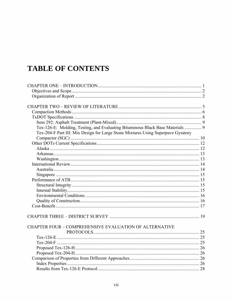
TABLE OF CONTENTS CHAPTER ONE – INTRODUCTION ........................................................................................... 1
Objectives and Scope .................................................................................................................. 2 Organization of Report ............................................................................................................... 2
CHAPTER TWO – REVIEW OF LITERATURE ......................................................................... 5
Compaction Methods .................................................................................................................. 6 TxDOT Specifications ................................................................................................................ 8
Item 292: Asphalt Treatment (Plant-Mixed) ........................................................................... 9 Tex-126-E: Molding, Testing, and Evaluating Bituminous Black Base Materials ............... 9 Tex-204-F Part III: Mix Design for Large Stone Mixtures Using Superpave Gyratory Compactor (SGC) ................................................................................................................. 10
Other DOTs Current Specifications .......................................................................................... 12 Alaska ................................................................................................................................... 12 Arkansas ................................................................................................................................ 13 Washington ........................................................................................................................... 13
International Review ................................................................................................................. 14 Australia ................................................................................................................................ 14 Singapore .............................................................................................................................. 15
Performance of ATB ................................................................................................................. 15 Structural Integrity ................................................................................................................ 15 Internal Stability .................................................................................................................... 15 Environmental Conditions .................................................................................................... 16 Quality of Construction......................................................................................................... 16
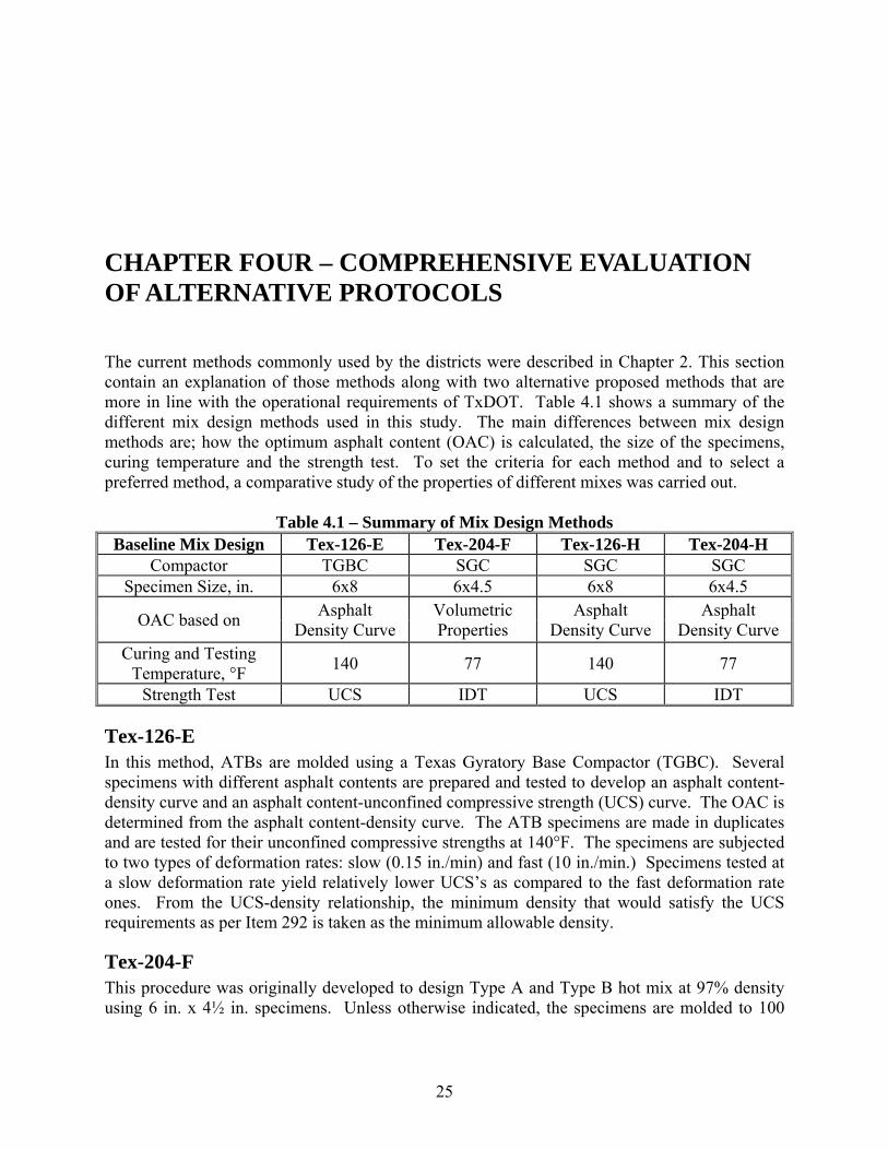
Cost-Benefit .............................................................................................................................. 17 CHAPTER THREE – DISTRICT SURVEY ............................................................................... 19 CHAPTER FOUR – COMPREHENSIVE EVALUATION OF ALTERNATIVE PROTOCOLS ............................................................................................. 25
Tex-126-E ............................................................................................................................. 25 Tex-204-F ............................................................................................................................. 25 Proposed Tex-126-H ............................................................................................................. 26 Proposed Tex-204-H ............................................................................................................. 26
Comparison of Properties from Different Approaches ............................................................. 26 Index Properties .................................................................................................................... 26 Results from Tex-126-E Protocol ......................................................................................... 28

viii
Results from Tex-126-H Protocol ......................................................................................... 30 Results from Tex-204-H Protocol ......................................................................................... 32
Tex-204-F ................................................................................................................................. 34 Moisture Susceptibility ............................................................................................................. 36 Analysis of Results ................................................................................................................... 37
CHAPTER FIVE – EVALUATION OF PARAMETERS THAT IMPACT PERFORMANCE. 45
Impact of Number of Gyrations ................................................................................................ 45 Tex-126-H Protocol .............................................................................................................. 45 Tex-204-H Protocol .............................................................................................................. 50
Impact of Curing Temperature .................................................................................................. 53 Tex-126-H Protocol .............................................................................................................. 53 Tex-204-H Protocol .............................................................................................................. 55
Impact of Binder Grade ............................................................................................................ 55 Tex-126-H Protocol .............................................................................................................. 55 Tex- 204-H Protocol ............................................................................................................. 60
Impact of AC Content ............................................................................................................... 60 Impact of Gradation .................................................................................................................. 60
Tex-126-H Protocol .............................................................................................................. 60 Tex-204-H Protocol .............................................................................................................. 66 Proposed Mix Design Protocol ............................................................................................. 70
Determination of OAC .............................................................................................................. 71 CHAPTER SIX – FIELD PERFORMANCE MONITORING .................................................... 73
Laboratory Results ................................................................................................................ 73 Plant-Mixed Materials .......................................................................................................... 76 Field Observations and Activities ......................................................................................... 78 Comparison of Laboratory and Field Results ....................................................................... 81 Recommendation on Construction Specifications ................................................................ 86
CHAPTER SEVEN – COST BENEFIT ANALYSIS .................................................................. 87
Laboratory Results for Type B Materials ................................................................................. 87 Plant-Mixed Materials .......................................................................................................... 87
Field Cores ................................................................................................................................ 88 Field Results.......................................................................................................................... 90
Performance of ATB and Type B Mix Materials ..................................................................... 90 Cost Comparison ....................................................................................................................... 95
CHAPTER EIGHT – CLOSURE ................................................................................................. 99 REFERENCE .................................................................................................................. 101 Appendix A – QUESTIONNAIRE ........................................................................................... 103 Appendix B – TEX-204-H TEST PROCEDURE ..................................................................... 109
ix
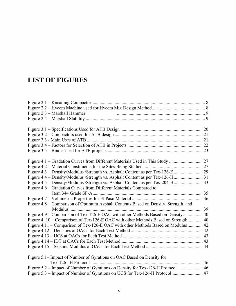
LIST OF FIGURES
Figure 2.1 – Kneading Compactor .................................................................................................. 8 Figure 2.2 – Hveem Machine used for Hveem Mix Design Method .............................................. 8 Figure 2.3 – Marshall Hammer ............................................................................ 9 Figure 2.4 – Marshall Stability ....................................................................................................... 9 Figure 3.1 – Specifications Used for ATB Design ....................................................................... 20 Figure 3.2 – Compactors used for ATB design ............................................................................ 21 Figure 3.3 - Main Uses of ATB .................................................................................................... 21 Figure 3.4 – Factors for Selection of ATB in Projects ................................................................. 22 Figure 3.5 – Binder used for ATB projects ................................................................................... 23 Figure 4.1 – Gradation Curves from Different Materials Used in This Study ............................. 27 Figure 4.2 – Material Constituents for the Sites Being Studied ................................................... 27 Figure 4.3 – Density/Modulus /Strength vs. Asphalt Content as per Tex-126-E ......................... 29 Figure 4.4 – Density/Modulus /Strength vs. Asphalt Content as per Tex-126-H ......................... 31 Figure 4.5 – Density/Modulus /Strength vs. Asphalt Content as per Tex-204-H ......................... 33 Figure 4.6 – Gradation Curves from Different Materials Compared to
Item 344 Grade SP-A ............................................................................................... 35 Figure 4.7 – Volumetric Properties for El Paso Material ............................................................. 36 Figure 4.8 – Comparison of Optimum Asphalt Contents Based on Density, Strength, and Modulus ................................................................................................................... 39 Figure 4.9 – Comparison of Tex-126-E OAC with other Methods Based on Density ................. 40 Figure 4. 10 – Comparison of Tex-126-E OAC with other Methods Based on Strength ............. 40 Figure 4.11 – Comparison of Tex-126-E OAC with other Methods Based on Modulus ............. 42 Figure 4.12 – Densities at OACs for Each Test Method .............................................................. 42 Figure 4.13 – UCS at OACs for Each Test Method ..................................................................... 43 Figure 4.14 – IDT at OACs for Each Test Method ....................................................................... 43 Figure 4.15 – Seismic Modulus at OACs for Each Test Method ................................................. 44 Figure 5.1– Impact of Number of Gyrations on OAC Based on Density for Tex-126 –H Protocol ................................................................................................. 46 Figure 5.2 – Impact of Number of Gyrations on Density for Tex-126-H Protocol ...................... 46 Figure 5.3 – Impact of Number of Gyrations on UCS for Tex-126-H Protocol ........................... 47

x
Figure 5.4 – Impact of Number of Gyrations on Modulus for Tex-126-H Protocol .................... 47 Figure 5.5 – Locking Points for Tex-126-H and Tex-126-E Specimens ...................................... 48 Figure 5.6 – Comparison of Density from Tex-126-E and Tex-126-H Protocols ........................ 49 Figure 5.7 – Impact of Number of Gyrations on OAC for Tex-204-H Protocol .......................... 50 Figure 5.8 – Impact of Number of Gyrations on Density for Tex-204-H Protocol ...................... 51 Figure 5.9 – Impact of Number of Gyrations on IDT Strength for Tex-204-H Protocol ............. 51 Figure 5.10 – Impact of Number of Gyrations on Modulus for Tex-204-H Protocol .................. 52 Figure 5.11 – Comparison of Density from Tex-126-E and Tex-204-H Protocols ...................... 53 Figure 5.12 – Impact of Curing Temperature on UCS for Tex-126-H Protocol .......................... 54 Figure 5.13 – Impact of Curing Temperature on Modulus for Tex-126-H Protocol .................... 54 Figure 5.14 – Comparison of Strengths from Different Curing Regimes using Tex-126-H Specimens with Those from Tex-126-E .............................................. 56 Figure 5.15 – Comparison of Strengths from Different Curing Regimes using Tex-126-E Specimens ............................................................................................ 56 Figure 5.16 – Impact of Curing Temperature on IDT Strength for Tex-204-H Protocol ............. 57 Figure 5.17 – Impact of Curing Temperature on Modulus for Tex-204-H Protocol .................... 57 Figure 5.18 – Comparison of Strengths from Different Curing Regimes using Tex-204-H Specimens ............................................................................................ 58 Figure 5.19 – Impact of Binder Grade on OAC based on Density for Tex-126-H Protocol ........ 58 Figure 5.20 – Impact of Binder Grade on Density for Tex-126-H Protocol ................................. 59 Figure 5.21 – Impact of Binder Grade on UCS for Tex-126-H Protocol ..................................... 59 Figure 5.22 – Impact of Binder Grade on OAC for Tex-204-H Protocol ..................................... 61 Figure 5.23 – Impact of Binder Grade on Density for Tex-204-H Protocol ................................. 61 Figure 5.24 – Impact of Binder Grade on IDT Strength for Tex-204-H Protocol ........................ 62 Figure 5.25 – Impact of Binder Grade on Modulus for Tex-204-H Protocol ............................... 62 Figure 5.26 – Impact of Asphalt Content Variation on UCS for Tex-126-H Protocol ................. 63 Figure 5.27 – Impact of Asphalt Content Variation on Modulus for Tex-126-H Protocol .......... 63 Figure 5.28 – Impact of Asphalt Content Variation on IDT for Tex-204-H Protocol .................. 64 Figure 5.29 – Impact of Asphalt Content Variation on Modulus for Tex-204-H Protocol .......... 64 Figure 5.30 – Impact of Fines Content Variation on OAC Tex-204-H Protocol ......................... 65 Figure 5.31 – Impact of Fines Content Variation on Density Tex-204-H Protocol ..................... 66 Figure 5.32 – Impact of Fines Content Variation on UCS Tex-126-H Protocol .......................... 67 Figure 5.33 – Impact of Fines Content Variation on Modulus for Tex-126-H Protocol .............. 67 Figure 5.34 – Impact of Fines Content Variation on OAC for Tex-204-H .................................. 68 Figure 5.35 – Impact of Fines Content Variation on Density for Tex-204-H .............................. 68 Figure 5.36 – Impact of Fines Content Variation on IDT for Tex-204-H .................................... 69 Figure 5.37 – Impact of Fines Content Variation on Modulus for Tex-204-H ............................. 69 Figure 5.38 – Density/IDT Asphalt Content Combined Curves ................................................... 72 Figure 5.39 – Relative Density/IDT Asphalt Content Combined Curves .................................... 72 Figure 6.1 – Locations of Sites Visited used in this Study ........................................................... 74 Figure 6.2 – Pavement Profiles for Sites Visited in this Study ..................................................... 75 Figure 6.3 – Laboratory Gradation Curves for Alpine, Beaumont and Houston Materials .......... 75 Figure 6.4 – Density/ Strength vs. Asphalt Content for Alpine Material ..................................... 77 Figure 6.5 – Density/ Strength vs. Asphalt Content for Houston Material ................................... 77 Figure 6.6 – Density/ Strength vs. Asphalt Content for Beaumont Material ................................ 77
xi
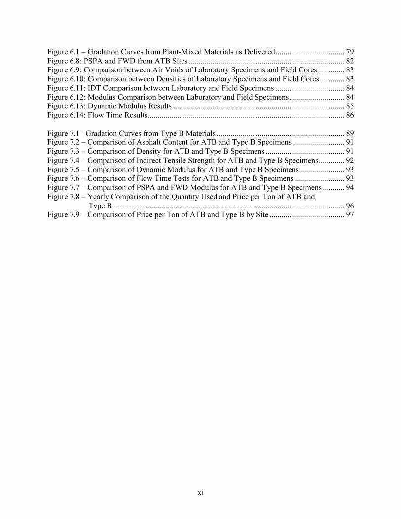
Figure 6.1 – Gradation Curves from Plant-Mixed Materials as Delivered ................................... 79 Figure 6.8: PSPA and FWD from ATB Sites ............................................................................... 82 Figure 6.9: Comparison between Air Voids of Laboratory Specimens and Field Cores ............. 83 Figure 6.10: Comparison between Densities of Laboratory Specimens and Field Cores ............ 83 Figure 6.11: IDT Comparison between Laboratory and Field Specimens ................................... 84 Figure 6.12: Modulus Comparison between Laboratory and Field Specimens ............................ 84 Figure 6.13: Dynamic Modulus Results ....................................................................................... 85 Figure 6.14: Flow Time Results.................................................................................................... 86 Figure 7.1 –Gradation Curves from Type B Materials ................................................................. 89 Figure 7.2 – Comparison of Asphalt Content for ATB and Type B Specimens .......................... 91 Figure 7.3 – Comparison of Density for ATB and Type B Specimens ........................................ 91 Figure 7.4 – Comparison of Indirect Tensile Strength for ATB and Type B Specimens ............. 92 Figure 7.5 – Comparison of Dynamic Modulus for ATB and Type B Specimens ....................... 93 Figure 7.6 – Comparison of Flow Time Tests for ATB and Type B Specimens ......................... 93 Figure 7.7 – Comparison of PSPA and FWD Modulus for ATB and Type B Specimens ........... 94 Figure 7.8 – Yearly Comparison of the Quantity Used and Price per Ton of ATB and Type B ...................................................................................................................... 96 Figure 7.9 – Comparison of Price per Ton of ATB and Type B by Site ...................................... 97

xii
xiii
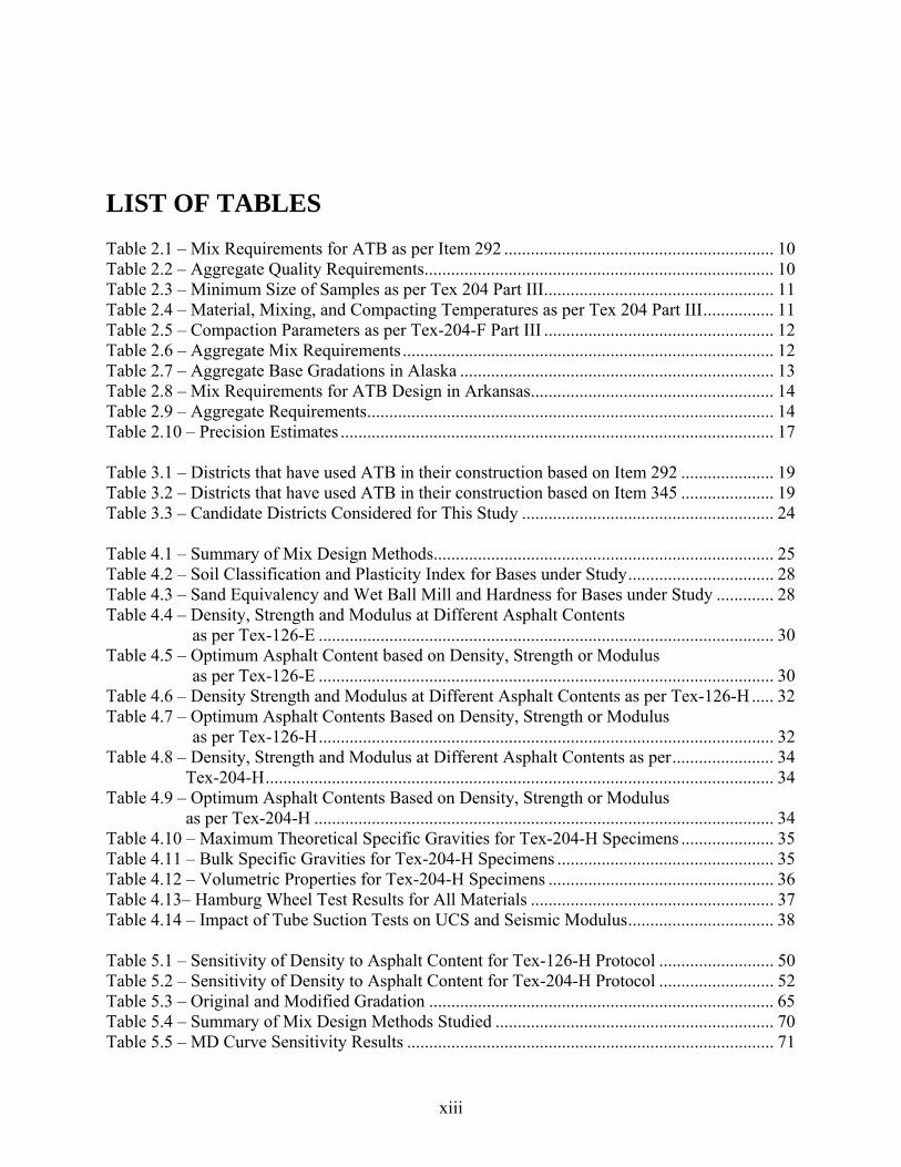
LIST OF TABLES Table 2.1 – Mix Requirements for ATB as per Item 292 ............................................................. 10 Table 2.2 – Aggregate Quality Requirements ............................................................................... 10 Table 2.3 – Minimum Size of Samples as per Tex 204 Part III .................................................... 11 Table 2.4 – Material, Mixing, and Compacting Temperatures as per Tex 204 Part III ................ 11 Table 2.5 – Compaction Parameters as per Tex-204-F Part III .................................................... 12 Table 2.6 – Aggregate Mix Requirements .................................................................................... 12 Table 2.7 – Aggregate Base Gradations in Alaska ....................................................................... 13 Table 2.8 – Mix Requirements for ATB Design in Arkansas ....................................................... 14 Table 2.9 – Aggregate Requirements ............................................................................................ 14 Table 2.10 – Precision Estimates .................................................................................................. 17 Table 3.1 – Districts that have used ATB in their construction based on Item 292 ..................... 19 Table 3.2 – Districts that have used ATB in their construction based on Item 345 ..................... 19 Table 3.3 – Candidate Districts Considered for This Study ......................................................... 24 Table 4.1 – Summary of Mix Design Methods ............................................................................. 25 Table 4.2 – Soil Classification and Plasticity Index for Bases under Study ................................. 28 Table 4.3 – Sand Equivalency and Wet Ball Mill and Hardness for Bases under Study ............. 28 Table 4.4 – Density, Strength and Modulus at Different Asphalt Contents as per Tex-126-E ....................................................................................................... 30 Table 4.5 – Optimum Asphalt Content based on Density, Strength or Modulus as per Tex-126-E ....................................................................................................... 30 Table 4.6 – Density Strength and Modulus at Different Asphalt Contents as per Tex-126-H ..... 32 Table 4.7 – Optimum Asphalt Contents Based on Density, Strength or Modulus as per Tex-126-H ....................................................................................................... 32 Table 4.8 – Density, Strength and Modulus at Different Asphalt Contents as per ....................... 34 Tex-204-H ................................................................................................................... 34 Table 4.9 – Optimum Asphalt Contents Based on Density, Strength or Modulus as per Tex-204-H ........................................................................................................ 34 Table 4.10 – Maximum Theoretical Specific Gravities for Tex-204-H Specimens ..................... 35 Table 4.11 – Bulk Specific Gravities for Tex-204-H Specimens ................................................. 35 Table 4.12 – Volumetric Properties for Tex-204-H Specimens ................................................... 36 Table 4.13– Hamburg Wheel Test Results for All Materials ....................................................... 37 Table 4.14 – Impact of Tube Suction Tests on UCS and Seismic Modulus ................................. 38 Table 5.1 – Sensitivity of Density to Asphalt Content for Tex-126-H Protocol .......................... 50 Table 5.2 – Sensitivity of Density to Asphalt Content for Tex-204-H Protocol .......................... 52 Table 5.3 – Original and Modified Gradation .............................................................................. 65 Table 5.4 – Summary of Mix Design Methods Studied ............................................................... 70 Table 5.5 – MD Curve Sensitivity Results ................................................................................... 71
xiv
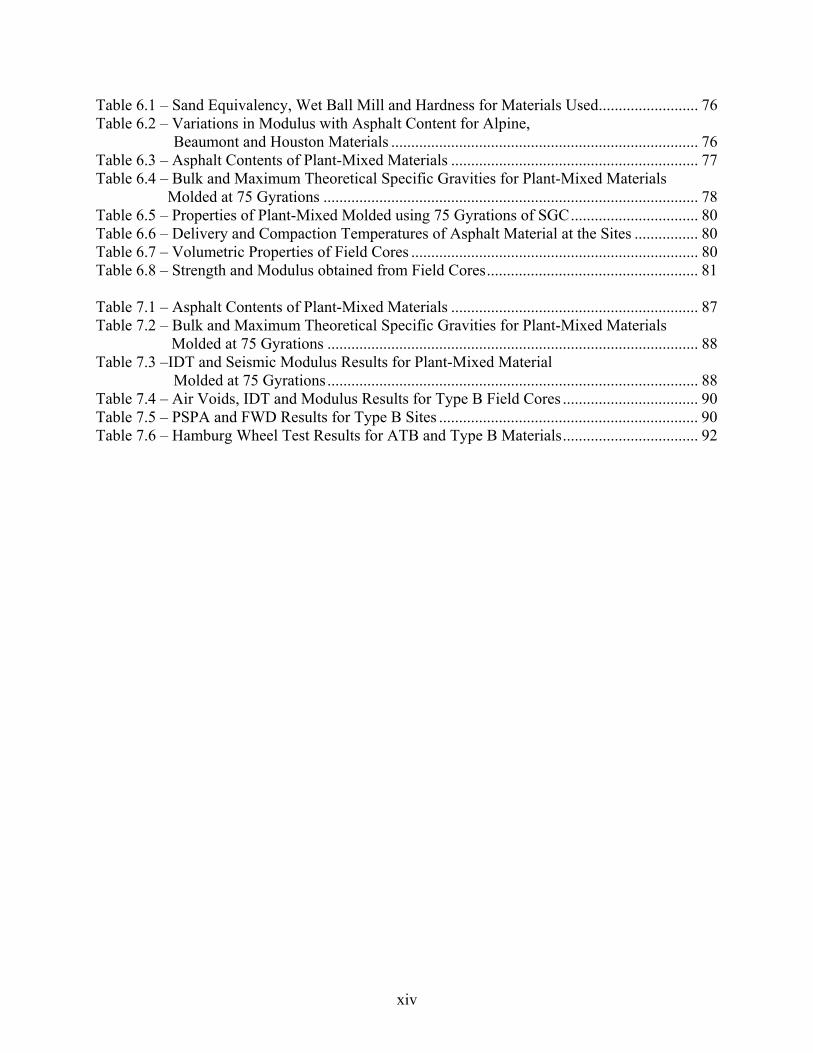
Table 6.1 – Sand Equivalency, Wet Ball Mill and Hardness for Materials Used ......................... 76 Table 6.2 – Variations in Modulus with Asphalt Content for Alpine, Beaumont and Houston Materials ............................................................................. 76 Table 6.3 – Asphalt Contents of Plant-Mixed Materials .............................................................. 77 Table 6.4 – Bulk and Maximum Theoretical Specific Gravities for Plant-Mixed Materials Molded at 75 Gyrations .............................................................................................. 78 Table 6.5 – Properties of Plant-Mixed Molded using 75 Gyrations of SGC ................................ 80 Table 6.6 – Delivery and Compaction Temperatures of Asphalt Material at the Sites ................ 80 Table 6.7 – Volumetric Properties of Field Cores ........................................................................ 80 Table 6.8 – Strength and Modulus obtained from Field Cores ..................................................... 81 Table 7.1 – Asphalt Contents of Plant-Mixed Materials .............................................................. 87 Table 7.2 – Bulk and Maximum Theoretical Specific Gravities for Plant-Mixed Materials Molded at 75 Gyrations ............................................................................................. 88 Table 7.3 –IDT and Seismic Modulus Results for Plant-Mixed Material Molded at 75 Gyrations ............................................................................................. 88 Table 7.4 – Air Voids, IDT and Modulus Results for Type B Field Cores .................................. 90 Table 7.5 – PSPA and FWD Results for Type B Sites ................................................................. 90 Table 7.6 – Hamburg Wheel Test Results for ATB and Type B Materials .................................. 92
1
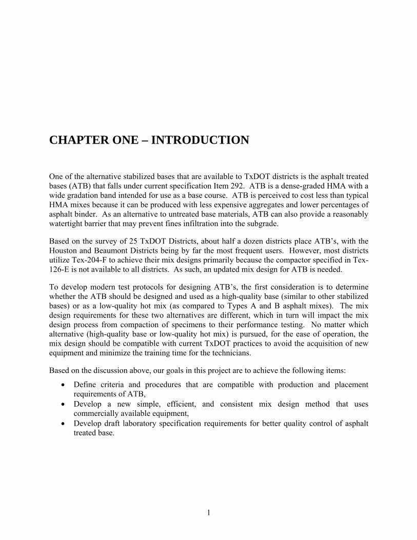
CHAPTER ONE – INTRODUCTION
One of the alternative stabilized bases that are available to TxDOT districts is the asphalt treated bases (ATB) that falls under current specification Item 292. ATB is a dense-graded HMA with a wide gradation band intended for use as a base course. ATB is perceived to cost less than typical HMA mixes because it can be produced with less expensive aggregates and lower percentages of asphalt binder. As an alternative to untreated base materials, ATB can also provide a reasonably watertight barrier that may prevent fines infiltration into the subgrade.
Based on the survey of 25 TxDOT Districts, about half a dozen districts place ATB’s, with the Houston and Beaumont Districts being by far the most frequent users. However, most districts utilize Tex-204-F to achieve their mix designs primarily because the compactor specified in Tex-126-E is not available to all districts. As such, an updated mix design for ATB is needed.
To develop modern test protocols for designing ATB’s, the first consideration is to determine whether the ATB should be designed and used as a high-quality base (similar to other stabilized bases) or as a low-quality hot mix (as compared to Types A and B asphalt mixes). The mix design requirements for these two alternatives are different, which in turn will impact the mix design process from compaction of specimens to their performance testing. No matter which alternative (high-quality base or low-quality hot mix) is pursued, for the ease of operation, the mix design should be compatible with current TxDOT practices to avoid the acquisition of new equipment and minimize the training time for the technicians.
Based on the discussion above, our goals in this project are to achieve the following items:
Define criteria and procedures that are compatible with production and placement requirements of ATB,
Develop a new simple, efficient, and consistent mix design method that uses commercially available equipment,
Develop draft laboratory specification requirements for better quality control of asphalt treated base.
2
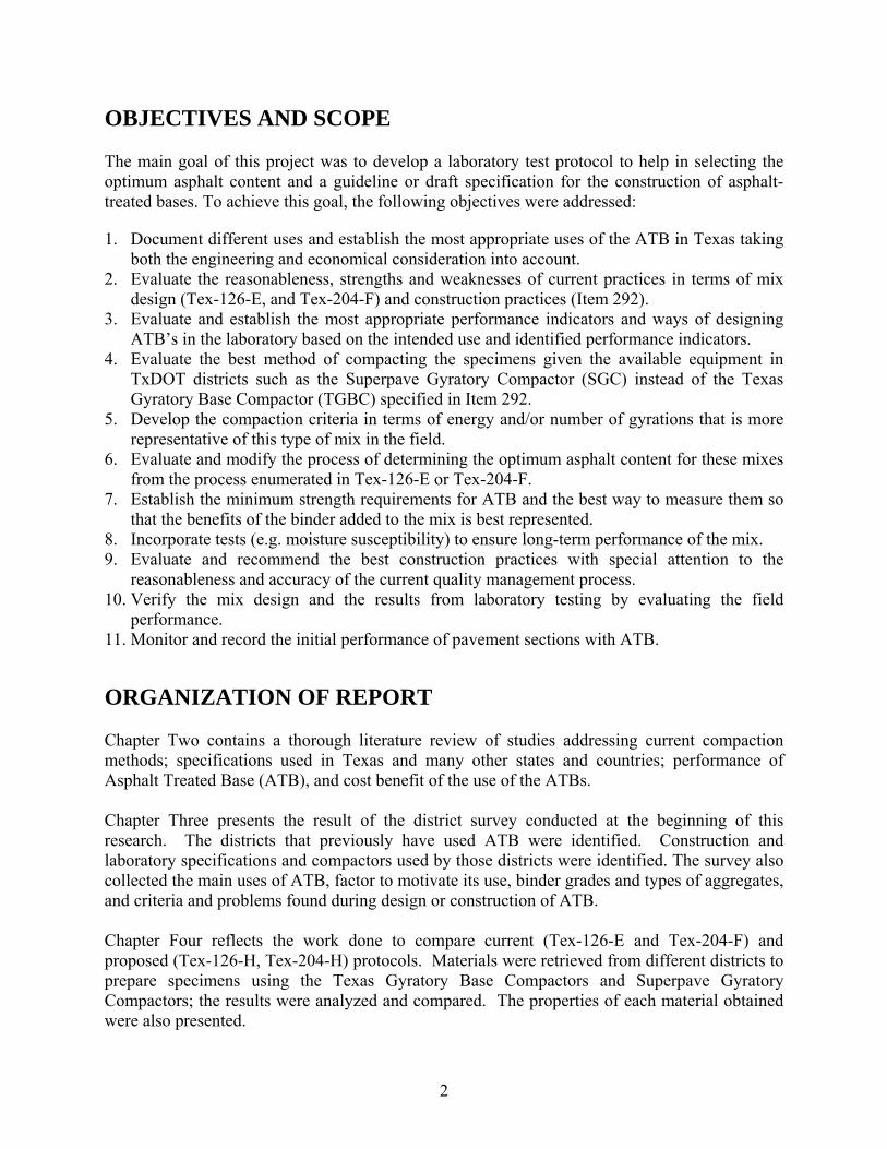
OBJECTIVES AND SCOPE The main goal of this project was to develop a laboratory test protocol to help in selecting the optimum asphalt content and a guideline or draft specification for the construction of asphalt-treated bases. To achieve this goal, the following objectives were addressed:
1. Document different uses and establish the most appropriate uses of the ATB in Texas taking both the engineering and economical consideration into account.
2. Evaluate the reasonableness, strengths and weaknesses of current practices in terms of mix design (Tex-126-E, and Tex-204-F) and construction practices (Item 292).
3. Evaluate and establish the most appropriate performance indicators and ways of designing ATB’s in the laboratory based on the intended use and identified performance indicators.
4. Evaluate the best method of compacting the specimens given the available equipment in TxDOT districts such as the Superpave Gyratory Compactor (SGC) instead of the Texas Gyratory Base Compactor (TGBC) specified in Item 292.
5. Develop the compaction criteria in terms of energy and/or number of gyrations that is more representative of this type of mix in the field.
6. Evaluate and modify the process of determining the optimum asphalt content for these mixes from the process enumerated in Tex-126-E or Tex-204-F.
7. Establish the minimum strength requirements for ATB and the best way to measure them so that the benefits of the binder added to the mix is best represented.
8. Incorporate tests (e.g. moisture susceptibility) to ensure long-term performance of the mix. 9. Evaluate and recommend the best construction practices with special attention to the
reasonableness and accuracy of the current quality management process. 10. Verify the mix design and the results from laboratory testing by evaluating the field
performance. 11. Monitor and record the initial performance of pavement sections with ATB.
ORGANIZATION OF REPORT Chapter Two contains a thorough literature review of studies addressing current compaction methods; specifications used in Texas and many other states and countries; performance of Asphalt Treated Base (ATB), and cost benefit of the use of the ATBs. Chapter Three presents the result of the district survey conducted at the beginning of this research. The districts that previously have used ATB were identified. Construction and laboratory specifications and compactors used by those districts were identified. The survey also collected the main uses of ATB, factor to motivate its use, binder grades and types of aggregates, and criteria and problems found during design or construction of ATB. Chapter Four reflects the work done to compare current (Tex-126-E and Tex-204-F) and proposed (Tex-126-H, Tex-204-H) protocols. Materials were retrieved from different districts to prepare specimens using the Texas Gyratory Base Compactors and Superpave Gyratory Compactors; the results were analyzed and compared. The properties of each material obtained were also presented.
3
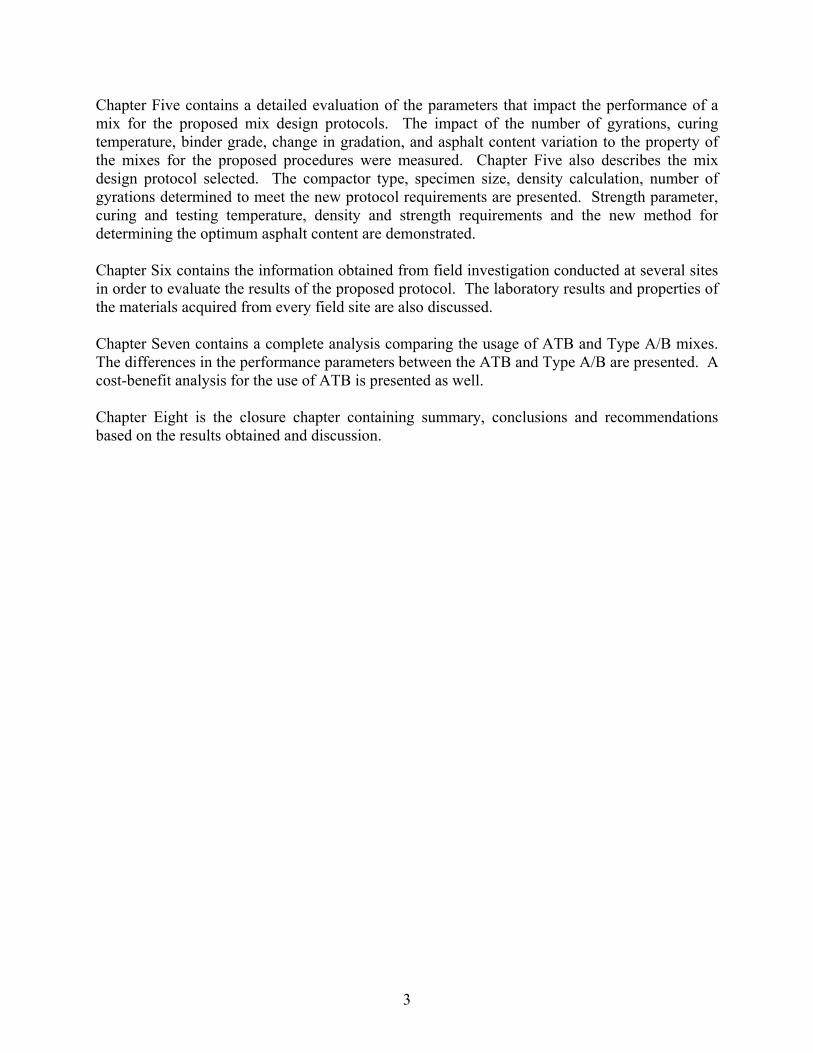
Chapter Five contains a detailed evaluation of the parameters that impact the performance of a mix for the proposed mix design protocols. The impact of the number of gyrations, curing temperature, binder grade, change in gradation, and asphalt content variation to the property of the mixes for the proposed procedures were measured. Chapter Five also describes the mix design protocol selected. The compactor type, specimen size, density calculation, number of gyrations determined to meet the new protocol requirements are presented. Strength parameter, curing and testing temperature, density and strength requirements and the new method for determining the optimum asphalt content are demonstrated. Chapter Six contains the information obtained from field investigation conducted at several sites in order to evaluate the results of the proposed protocol. The laboratory results and properties of the materials acquired from every field site are also discussed. Chapter Seven contains a complete analysis comparing the usage of ATB and Type A/B mixes. The differences in the performance parameters between the ATB and Type A/B are presented. A cost-benefit analysis for the use of ATB is presented as well. Chapter Eight is the closure chapter containing summary, conclusions and recommendations based on the results obtained and discussion.

4
5
CHAPTER TWO – REVIEW OF LITERATURE The performance of a pavement depends on many factors such as the properties of the materials used, structural capacity of the pavement, construction method, traffic loading, and climatic conditions. For flexible pavements, the quality of the base layer is one of the most important factors. Previous research has found that much of the distress that flexible pavements experience can be traced to problems encountered in the base (Saeed et al., 2001). The use of a cost efficient base layer, that would extend the pavement life, that would require less thickness, or that would use local materials, is highly desirable. Asphalt-treated bases (ATB) fit this category. According to the National Asphalt Pavement Association (NAPA), (http://training.ce.washington.edu/wsdot/Modules/02_pavement_types/02-3_body.htm), ATB is a dense-graded hot mix asphalt (HMA) with a wide gradation band with a lower asphalt content that can be used as a base course. Among the features that make it different from HMA are (Wong et al., 2004):
1) HMA layer may receive direct impact from traffic and experience more serious weather conditions than those experienced by the ATB
2) Thickness of ATB is greater than the one of the HMA One of the main problems with semi-rigid pavement structures is transverse cracking in the stabilized base and the related propagation of cracks to the surface, which diminishes the life of pavements. In these cases, the ATB may be more flexible and resistant to fatigue cracking as compared to cement stabilized bases (Dykman et al., 2003). Besides new construction, ATB can be beneficial in rehabilitation projects as well. According to Dykman et al. (2003), the crucial factors in choosing ATB as a way of rehabilitation are:
Quick construction time, therefore decreased delays and diminished traffic disturbance Low permeability to moderate pore water pressure effect (Cedergren, 1977) Minimal moisture sensitivity as a consequence of moisture ingress Quite flexible, consequently decrease the possibility of reflective cracking (Marks and
Heisman, 1985.) Research related to ATB has been limited even though ATB has been used as structural pavement layer for more than 40 years (Dykman et al., 2003). McDowell and Smith (1969) performed the first comprehensive study in the design and construction of ATB (also known as
6
black base). An important objective of their study was to observe the effects of loading rate on the unconfined compressive strength (UCS) of ATB. McDowell and Smith used loading rates of 6, 8, 10 and 15 in./min, noticing that when testing at fast rates of loading a definite improvement in compressive strength of asphalt treated materials over untreated materials was obtained. They stated that a fast rate of loading test should become part of the analysis of asphalt mixtures. McDowell and Smith (1969) also studied the effects of moisture absorption on strength and its relation to total percent voids. They used pressure pycnometer to obtain saturation in the least amount of time. They concluded that mixtures having less than 5.5% total voids will possibly not lose strength due to absorption of moisture. While McDowell and Smith investigation was taking place, the Texas Gyratory Compactor (TGC) was revised so that 6 in. in diameter by 8 in. in height specimens could be prepared.
Compaction Methods An analysis of the specifications of all fifty highway agencies that are incorporated in the Federal Highway Administration (FHWA) National Highway Specifications indicates that most highway agencies either support designing the ATB using the HMA specifications (e.g., Illinois, Indiana, Washington), or utilizing emulsion rather than asphalt (e.g., Delaware, Maine, Maryland). However, several transportation agencies are upgrading their conventional compaction methods such as TGC or Marshall with SGC for routine mix design. According to Button et al. (2006) the advantages of using the SGC include the following items:
Its ability to estimate the compatibility of mixes from density during the compaction process
Its ability to identify weak aggregate structures that collapse very quickly to lower air voids
Improved reproducibility of samples due to mostly mechanical control of compaction process
Ability to simulate field compacted mixes relatively better than other compaction methods
Gyratory compaction was originally created in 1939 by the Texas Highway Department to help in the molding and design of asphalt mixtures (Harman et al., 2002). Gyratory compactors were designed to simulate the orientation of aggregate, degradation of aggregate, field compaction, and traffic degradation that occurs in HMA during production, compaction and traffic loading (Collins et al., 1997). Dykman et al. (2003) state that gyratory compaction can simulate the action of a roller in the field due to its capability to rotate the principal stresses. On the other hand, gyratory compaction can create totally different compaction characteristics. These characteristics depend on the adjustment and calibration of several parameters that affect the degree of compaction of laboratory HMA specimens (Mokwa et al., 2008). According to Button et al. (2006), the lower angle of gyration of the SGC (1.25°) imparts significantly less mechanical energy into the specimen per gyration as compared to the TGBC (5.8° gyration angle). Different angles of gyration have different influence on the orientation of the aggregates, particularly the larger aggregates. The differences between specimens prepared using the TGBC and SGC, such as air void structure, aggregate orientation, voids in mineral
7
aggregate (VMA) and density gradient, will not likely be consistent because these differences will depend on the shear resistance of the mixture.
Mokwa et al. (2008) used confining pressures ranging from 30 psi to 90 psi in preparing specimens with a SGC. They found that mixes with smaller particles sizes exhibited higher rates of densification as a result of higher confining pressures. The confining pressure applied to the specimen according to Tex-126-E varies from 20 psi to 60 psi for the TGBC. Aguiar-Moya et al. (2007) indicate that the basis for the number of gyrations is that the compactive effort obtained in the laboratory should produce the same outcome on the asphalt mixtures (to increase density) as traffic loads for in-place asphalt mixes. As more weight is assigned to fatigue resistance, the optimum number of gyrations decreases, therefore producing mixes with higher binder contents. Similarly, as more significance is given to rutting, the optimal number of gyrations increases. Button et al. (2006) indicate that the design gyrations in SGC can be reduced below the initial recommendations without compromising rutting resistance of HMA mixtures.
Although the SGC can produce the same volume of air voids as the TGBC in a given mixture type, the resulting optimum asphalt contents and engineering properties of the compacted mixtures may be measurably different because of different aggregate orientations and different density gradients within the specimens (Button et al., 1994; Von Quintus et al., 1991). According to NAPA (http://training.ce.washington.edu/wsdot/Modules/05_mix_design/05-3_ body.htm) the Hveem method has been proven to produce quality HMA from which long-lasting pavements can be constructed. Hveem method has the following six main steps:
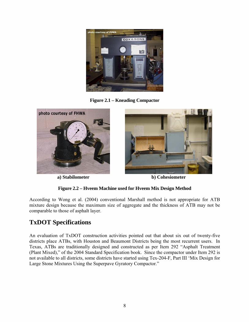
1. Aggregate selection 2. Asphalt binder selection 3. Sample preparation using the California Kneading Compactor (Figure 2.1) 4. Stability and cohesion determination using a Stabilometer and Cohesiometer (Figure 2.2) 5. Density and voids calculations, and 6. Optimum asphalt binder content selection.
The basic concept of the Marshall mix design method was originally developed by Bruce Marshall of the Mississippi Highway Department around 1939 and then refined by the U.S. Army. The Marshall method is very popular because of its relatively simplicity, economical equipment and proven record. Similar to Hveem method, the Marshall method consists of the following six basic steps:
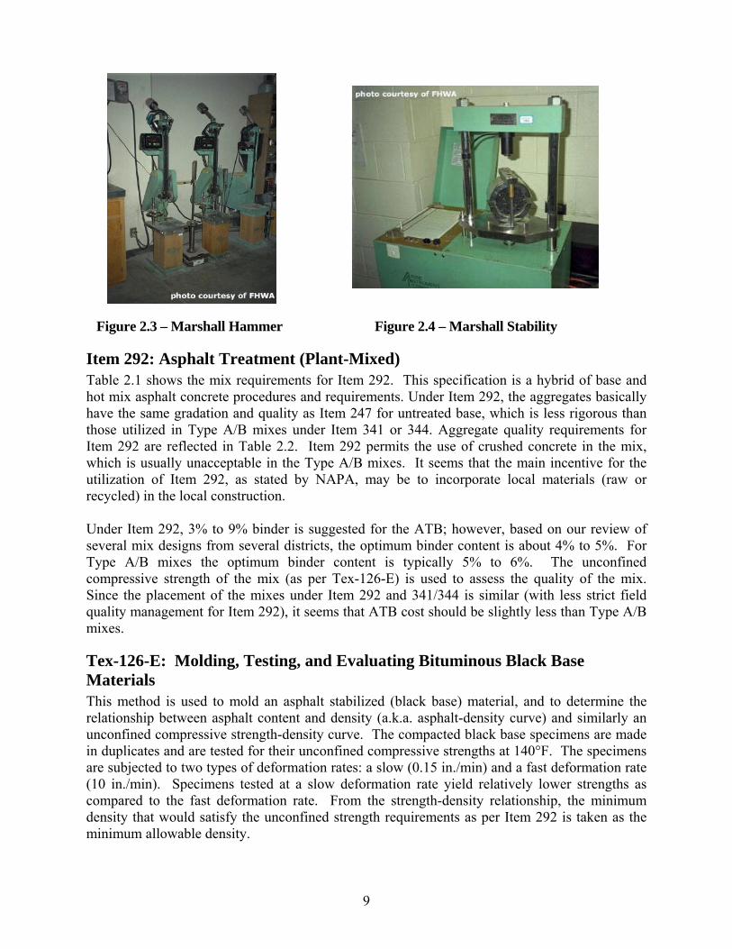
1. Aggregate selection 2. Asphalt binder selection 3. Sample preparation using the Marshall Hammer (Figure 2.3) 4. Stability and Flow Test using the Marshall Stability testing apparatus (Figure 2.4) 5. Density and voids calculations, and 6. Optimum asphalt binder content selection
8
Figure 2.1 – Kneading Compactor
a) Stabilometer b) Cohesiometer
Figure 2.2 – Hveem Machine used for Hveem Mix Design Method
According to Wong et al. (2004) conventional Marshall method is not appropriate for ATB mixture design because the maximum size of aggregate and the thickness of ATB may not be comparable to those of asphalt layer.
TxDOT Specifications An evaluation of TxDOT construction activities pointed out that about six out of twenty-five districts place ATBs, with Houston and Beaumont Districts being the most recurrent users. In Texas, ATBs are traditionally designed and constructed as per Item 292 “Asphalt Treatment (Plant Mixed),” of the 2004 Standard Specification book. Since the compactor under Item 292 is not available to all districts, some districts have started using Tex-204-F, Part III ‘Mix Design for Large Stone Mixtures Using the Superpave Gyratory Compactor.”
9
Figure 2.3 – Marshall Hammer Figure 2.4 – Marshall Stability
Item 292: Asphalt Treatment (Plant-Mixed) Table 2.1 shows the mix requirements for Item 292. This specification is a hybrid of base and hot mix asphalt concrete procedures and requirements. Under Item 292, the aggregates basically have the same gradation and quality as Item 247 for untreated base, which is less rigorous than those utilized in Type A/B mixes under Item 341 or 344. Aggregate quality requirements for Item 292 are reflected in Table 2.2. Item 292 permits the use of crushed concrete in the mix, which is usually unacceptable in the Type A/B mixes. It seems that the main incentive for the utilization of Item 292, as stated by NAPA, may be to incorporate local materials (raw or recycled) in the local construction. Under Item 292, 3% to 9% binder is suggested for the ATB; however, based on our review of several mix designs from several districts, the optimum binder content is about 4% to 5%. For Type A/B mixes the optimum binder content is typically 5% to 6%. The unconfined compressive strength of the mix (as per Tex-126-E) is used to assess the quality of the mix. Since the placement of the mixes under Item 292 and 341/344 is similar (with less strict field quality management for Item 292), it seems that ATB cost should be slightly less than Type A/B mixes.
Tex-126-E: Molding, Testing, and Evaluating Bituminous Black Base Materials This method is used to mold an asphalt stabilized (black base) material, and to determine the relationship between asphalt content and density (a.k.a. asphalt-density curve) and similarly an unconfined compressive strength-density curve. The compacted black base specimens are made in duplicates and are tested for their unconfined compressive strengths at 140°F. The specimens are subjected to two types of deformation rates: a slow (0.15 in./min) and a fast deformation rate (10 in./min). Specimens tested at a slow deformation rate yield relatively lower strengths as compared to the fast deformation rate. From the strength-density relationship, the minimum density that would satisfy the unconfined strength requirements as per Item 292 is taken as the minimum allowable density.

10
Table 2.1 – Mix Requirements for ATB as per Item 292
Master Gradation Bands Tex-200-F, Part I, % Passing by Weight
Sieve Size Grade 1 Grade 2 Grade 3 Grade 4 1-3/4" 100 100
As shown on the plans
1-1/2" 100 90-100 1" 90-100
3/8" 45-70 #4 30-55 25-55 #40 15-30 15-40 15-40
Strength Requirements
Slow strength, psi, min.1 50 40 30 30 2
1. At optimum asphalt content 2. Unless a higher minimum strength is shown on the plans
Table 2.2 – Aggregate Quality Requirements
Property Test Method Specification Requirement
Wet ball mill, % max Tex-116-E
50
Max increase, % passing #40 20
Liquid Limit, max Tex-104-E 40
Plasticity Index, max Tex-106-E 10
Sand Equivalent, % min Tex-203-F 40
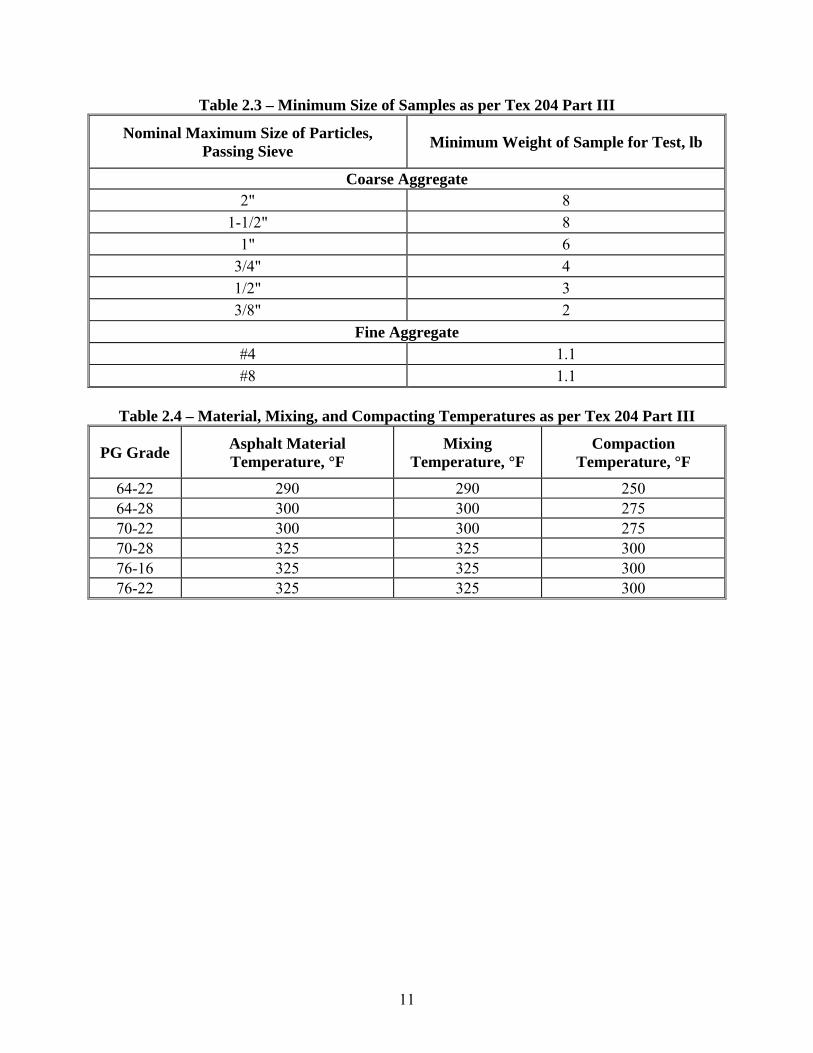
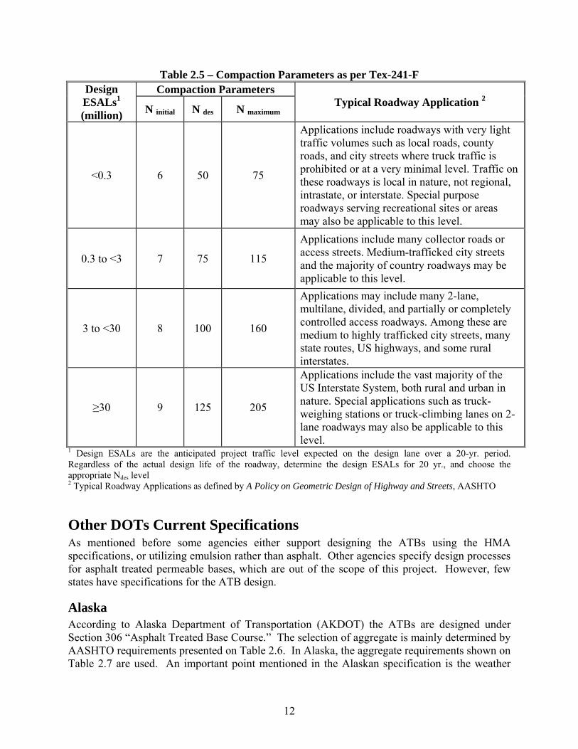
Tex-204-F Part III: Mix Design for Large Stone Mixtures Using Superpave Gyratory Compactor (SGC) This procedure was originally developed to design Type A and Type B hot mixes from a 6 in. by 4.5 in. specimen as per Table 2.3. Depending on the PG grade of the binder, the material, mixing, and compaction temperatures are according to Table 2.4. The specimens are molded to either 100 gyrations, or as shown on the plans, or as per Table 2.5. The specimens prepared under Tex-204-F are not the appropriate sizes for unconfined compressive strength (as per Tex-126-E). As such, the strength of the mix is assessed with the indirect tensile strength at a deformation rate of 2 in./min. at a temperature of 77 ± 2°F according to Tex-226-F.
11
Table 2.3 – Minimum Size of Samples as per Tex 204 Part III
Nominal Maximum Size of Particles, Passing Sieve
Minimum Weight of Sample for Test, lb
Coarse Aggregate 2" 8
1-1/2" 8 1" 6
3/4" 4 1/2" 3 3/8" 2
Fine Aggregate #4 1.1 #8 1.1
Table 2.4 – Material, Mixing, and Compacting Temperatures as per Tex 204 Part III
PG Grade Asphalt Material Temperature, °F
Mixing Temperature, °F
Compaction Temperature, °F
64-22 290 290 250 64-28 300 300 275 70-22 300 300 275 70-28 325 325 300 76-16 325 325 300 76-22 325 325 300
12
Table 2.5 – Compaction Parameters as per Tex-241-F Design ESALs1 (million)
Compaction Parameters Typical Roadway Application 2
N initial N des N maximum
<0.3 6 50 75
Applications include roadways with very light traffic volumes such as local roads, county roads, and city streets where truck traffic is prohibited or at a very minimal level. Traffic on these roadways is local in nature, not regional, intrastate, or interstate. Special purpose roadways serving recreational sites or areas may also be applicable to this level.
0.3 to <3 7 75 115
Applications include many collector roads or access streets. Medium-trafficked city streets and the majority of country roadways may be applicable to this level.
3 to <30 8 100 160
Applications may include many 2-lane, multilane, divided, and partially or completely controlled access roadways. Among these are medium to highly trafficked city streets, many state routes, US highways, and some rural interstates.
≥30 9 125 205
Applications include the vast majority of the US Interstate System, both rural and urban in nature. Special applications such as truck-weighing stations or truck-climbing lanes on 2-lane roadways may also be applicable to this level.
1 Design ESALs are the anticipated project traffic level expected on the design lane over a 20-yr. period. Regardless of the actual design life of the roadway, determine the design ESALs for 20 yr., and choose the appropriate Ndes level 2 Typical Roadway Applications as defined by A Policy on Geometric Design of Highway and Streets, AASHTO
Other DOTs Current Specifications As mentioned before some agencies either support designing the ATBs using the HMA specifications, or utilizing emulsion rather than asphalt. Other agencies specify design processes for asphalt treated permeable bases, which are out of the scope of this project. However, few states have specifications for the ATB design.
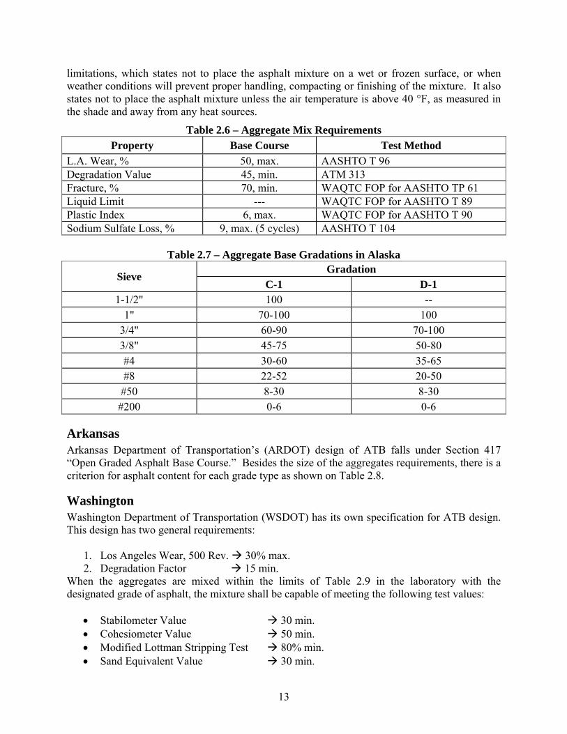
Alaska According to Alaska Department of Transportation (AKDOT) the ATBs are designed under Section 306 “Asphalt Treated Base Course.” The selection of aggregate is mainly determined by AASHTO requirements presented on Table 2.6. In Alaska, the aggregate requirements shown on Table 2.7 are used. An important point mentioned in the Alaskan specification is the weather
13
limitations, which states not to place the asphalt mixture on a wet or frozen surface, or when weather conditions will prevent proper handling, compacting or finishing of the mixture. It also states not to place the asphalt mixture unless the air temperature is above 40 °F, as measured in the shade and away from any heat sources.
Table 2.6 – Aggregate Mix Requirements
Property Base Course Test Method
L.A. Wear, % 50, max. AASHTO T 96 Degradation Value 45, min. ATM 313 Fracture, % 70, min. WAQTC FOP for AASHTO TP 61 Liquid Limit --- WAQTC FOP for AASHTO T 89 Plastic Index 6, max. WAQTC FOP for AASHTO T 90 Sodium Sulfate Loss, % 9, max. (5 cycles) AASHTO T 104
Table 2.7 – Aggregate Base Gradations in Alaska
Sieve Gradation
C-1 D-1 1-1/2" 100 --
1" 70-100 100 3/4" 60-90 70-100 3/8" 45-75 50-80 #4 30-60 35-65 #8 22-52 20-50 #50 8-30 8-30
#200 0-6 0-6
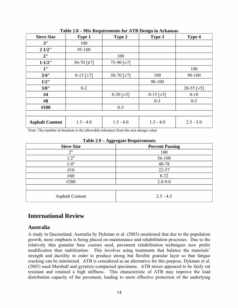
Arkansas Arkansas Department of Transportation’s (ARDOT) design of ATB falls under Section 417 “Open Graded Asphalt Base Course.” Besides the size of the aggregates requirements, there is a criterion for asphalt content for each grade type as shown on Table 2.8.
Washington Washington Department of Transportation (WSDOT) has its own specification for ATB design. This design has two general requirements:
1. Los Angeles Wear, 500 Rev. 30% max. 2. Degradation Factor 15 min.
When the aggregates are mixed within the limits of Table 2.9 in the laboratory with the designated grade of asphalt, the mixture shall be capable of meeting the following test values:
Stabilometer Value 30 min. Cohesiometer Value 50 min. Modified Lottman Stripping Test 80% min. Sand Equivalent Value 30 min.
14
Table 2.8 – Mix Requirements for ATB Design in Arkansas Sieve Size Type 1 Type 2 Type 3 Type 4
3" 100
2 1/2" 95-100
2" 100
1-1/2" 30-70 [±7] 75-90 [±7]
1" 100
3/4" 0-15 [±7] 50-70 [±7] 100 90-100
1/2" 90-100
3/8" 0-2 20-55 [±5]
#4 8-20 [±5] 0-15 [±5] 0-10
#8 0-3 0-5
#100 0-5
Asphalt Content 1.5 - 4.0 1.5 - 4.0 1.5 - 4.0 2.5 - 3.0
Note: The number in brackets is the allowable tolerance from the mix design value
Table 2.9 – Aggregate Requirements Sieve Size Percent Passing
2" 100 1/2" 56-100 1/4" 40-78 #10 22-57 #40 8-32 #200 2.0-9.0
Asphalt Content 2.5 - 4.5
International Review
Australia A study in Queensland, Australia by Dykman et al. (2003) mentioned that due to the population growth, more emphasis is being placed on maintenance and rehabilitation processes. Due to the relatively thin granular base courses used, pavement rehabilitation techniques now prefer modification than stabilization. This involves using treatments that balance the materials’ strength and ductility in order to produce strong but flexible granular layer so that fatigue cracking can be minimized. ATB is considered as an alternative for this purpose. Dykman et al. (2003) used Marshall and gyratory-compacted specimens. ATB mixes appeared to be fairly rut resistant and retained a high stiffness. This characteristic of ATB may improve the load distribution capacity of the pavement, leading to more effective protection of the underlying
15
layers. Dykman et al. (2003) and Ullman and Nolan (1991) conclude that the following benefits can be obtained from ATB, if used properly:
ATB can be placed with conventional equipment Fast construction Less cost than conventional hot-mix asphalt High stability Possibility of using marginal aggregates Potential for recycling
Singapore Wong et al. (2004) stated that ATB has better strength, stability, flexibility and durability as compared to common macadam base. Using ATB in highways with high traffic volume and increasing axle loading has been beneficial with respect to pavement performance. According to Wong et al., the determination of asphalt content for best performance is through establishing a balance between friction and cohesion. They recommended a procedure that considered the variations of the maximum density, indirect tensile strength and unconfined compressive strength of a mix to obtain the optimum mix design. Through static creep and fatigue tests, they demonstrated that mixture using their design method had good resistance to permanent deformation and fatigue at the bottom of the base. They prepared their specimens using an SGC, with the number of gyrations being based on the locking point of the mix. As a conclusion from that study, Wong et al. (2004) recommended the use of compression test and indirect tensile test for ATB design since these tests are simple and convenient.
Performance of ATB Some of the parameters that play an important role in the performance of the ATB as a system are the structural integrity of the section, the internal stability of the layer, the environmental conditions, and most importantly the quality of construction. Structural Integrity
The structural integrity of a flexible pavement section is controlled by several parameters. In most classical structural design programs (such as FPS19), the design thickness of the layers is (directly or indirectly) estimated based on the criteria that the stresses at the interfaces of the hot mix and base, and the base and subgrade, are low enough so that the cracking and rutting will not be an issue. The traffic volume is also a major consideration. For a given traffic condition, the thicker the layers overlying the base is, the thicker the base layer and the stiffer the subgrade are, the lower the base layer stresses will be. This indicates that not only the quality of base should be considered, the stiffness of the subgrade, and the thickness of the hot mix should also be considered. The complex modulus or diameteral resilient modulus tests can be performed for this purpose.
Internal Stability
The internal stability is defined as the excessive deformation of the base under the load. This manifests as rutting primarily associated with the base layer. To address this issue, repeated load permanent deformation lab tests as advocated by the FHWA should be used in conjunction with
16
the appropriate models that predicts the rutting of the hot-mix, base, and subgrade layers individually.
Environmental Conditions
The main environmental parameter of interest is the adverse effects of moisture and temperature on the strength and modulus of the base. Therefore, the importance of considering the impact of moisture on the performance of the material should not be neglected. Hamburg wheel tracking device, perhaps with some relaxed requirements, can be used for this purpose. Alternatively, two inter-related methods can be used to assess the impact of moisture on the performance of the base: Tube Suction Test (Tex-145) and the Free-Free Resonant Column (proposed Tex-147) or V-meter (proposed Tex-259). The Tube Suction Test (TST) qualitatively provides an estimate of the water-retention of the base material that can be correlated to the potential of damage to the base due to softening. The Free-Free Resonant Column (FFRC) or V-meter test is a quantitative nondestructive lab method that can be performed on a specimen for its modulus. In both methods, each specimen is oven-dried for two days and then allowed to soak moisture through capillary saturation. The modulus of the specimen is measured every day in conjunction with the tube suction test. The residual modulus corresponds to the modulus measured after the specimen soaked moisture for several days. Since the same specimen is used throughout for both TST and FFRC tests, the variation in moisture content with time can also be obtained by weighing the specimens daily. In that manner, the moisture retention properties of the material and its impact on modulus can be measured. Of course separate specimens should be prepared and tested for strength and modulus at optimum and after moisture conditioning to determine the retained strength and retained modulus for conventional design. Quality of Construction
No matter how much attention is focused on the mix design, the performance of the mix is directly related to the quality of construction. The necessity to perform a thorough evaluation of the component materials, and a thorough testing regimen and an aggressive quality control/ quality assurance program is well understood by TxDOT and is incorporated in the appropriate specifications. One of the major quality management tool used is the density of the in-place mat. To successfully assess the density of the mat, two parameters are necessary: The theoretical maximum specific gravity of the mixture (Tex-227-F) and the bulk specific gravity of the cores obtained from the finished mat (or density with the NDG) as per Tex-207-F. Both of these methods have been the subject of numerous studies by the federal and state highway agencies. There is some concern that the densities measured in those fashions may not be accurate or repeatable because of the nature of the base material (limited control on the gradation) used in ATBs. The most recent and comprehensive study of this matter has been carried out under a multi-year, multi-phase project (NCHRP 9-26) that was completed in 2007 by the AASHTO Materials Reference Laboratory (AMRL). The report from Phase 1 of the project included precision estimates of selected volumetric properties of HMA using non-absorptive aggregates
(Spellberg and Savage, 2003). The report from Phase 2 discusses the results of an investigation into the cause of variations in HMA bulk specific gravity test results using non-absorptive aggregates by Spellberg and Savage (2004). The report from Phase 3 includes a robust technique developed by AMRL for analyzing proficiency sample data for the purpose of obtaining reliable single-operator and multi-laboratory estimates of precision (Holsinger et al., 2005). The report
17
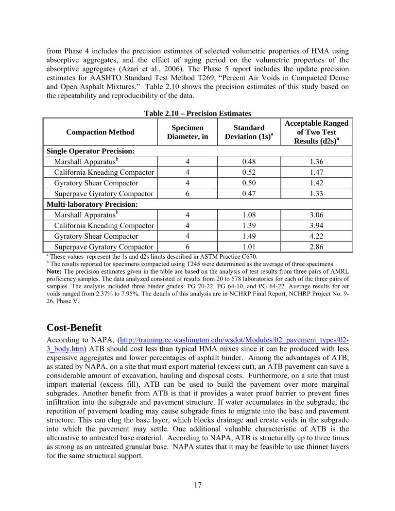
from Phase 4 includes the precision estimates of selected volumetric properties of HMA using absorptive aggregates, and the effect of aging period on the volumetric properties of the absorptive aggregates (Azari et al., 2006). The Phase 5 report includes the update precision estimates for AASHTO Standard Test Method T269, “Percent Air Voids in Compacted Dense and Open Asphalt Mixtures.” Table 2.10 shows the precision estimates of this study based on the repeatability and reproducibility of the data.
Table 2.10 – Precision Estimates
Compaction Method Specimen
Diameter, in Standard
Deviation (1s)a
Acceptable Ranged of Two Test
Results (d2s)a Single Operator Precision: Marshall Apparatusb 4 0.48 1.36 California Kneading Compactor 4 0.52 1.47 Gyratory Shear Compactor 4 0.50 1.42 Superpave Gyratory Compactor 6 0.47 1.33
Multi-laboratory Precision: Marshall Apparatusb 4 1.08 3.06 California Kneading Compactor 4 1.39 3.94 Gyratory Shear Compactor 4 1.49 4.22 Superpave Gyratory Compactor 6 1.01 2.86 a These values represent the 1s and d2s limits described in ASTM Practice C670. b The results reported for specimens compacted using T245 were determined as the average of three specimens. Note: The precision estimates given in the table are based on the analysis of test results from three pairs of AMRL proficiency samples. The data analyzed consisted of results from 20 to 578 laboratories for each of the three pairs of samples. The analysis included three binder grades: PG 70-22, PG 64-10, and PG 64-22. Average results for air voids ranged from 2.37% to 7.95%. The details of this analysis are in NCHRP Final Report, NCHRP Project No. 9-26, Phase V.
Cost-Benefit According to NAPA, (http://training.ce.washington.edu/wsdot/Modules/02_pavement_types/02-3_body.htm) ATB should cost less than typical HMA mixes since it can be produced with less expensive aggregates and lower percentages of asphalt binder. Among the advantages of ATB, as stated by NAPA, on a site that must export material (excess cut), an ATB pavement can save a considerable amount of excavation, hauling and disposal costs. Furthermore, on a site that must import material (excess fill), ATB can be used to build the pavement over more marginal subgrades. Another benefit from ATB is that it provides a water proof barrier to prevent fines infiltration into the subgrade and pavement structure. If water accumulates in the subgrade, the repetition of pavement loading may cause subgrade fines to migrate into the base and pavement structure. This can clog the base layer, which blocks drainage and create voids in the subgrade into which the pavement may settle. One additional valuable characteristic of ATB is the alternative to untreated base material. According to NAPA, ATB is structurally up to three times as strong as an untreated granular base. NAPA states that it may be feasible to use thinner layers for the same structural support.

18
In accordance with feedback from local authorities in Queensland, Australia, ATBs have performed very well over a period of ten years and in particular, its value for money when compared to other base stabilization treatments (Dykman et al., 2003). According to McDowell and Smith (1969) the economic benefit of ATB over other hot mixes is generally dependent on the use of local base materials, which do not have to be washed and sieved before batching.
19
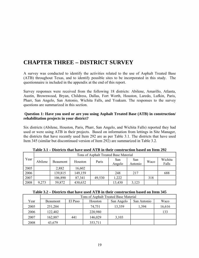
CHAPTER THREE – DISTRICT SURVEY A survey was conducted to identify the activities related to the use of Asphalt Treated Base (ATB) throughout Texas, and to identify possible sites to be incorporated in this study. The questionnaire is included in the appendix at the end of this report. Survey responses were received from the following 18 districts: Abilene, Amarillo, Atlanta, Austin, Brownwood, Bryan, Childress, Dallas, Fort Worth, Houston, Laredo, Lufkin, Paris, Pharr, San Angelo, San Antonio, Wichita Falls, and Yoakum. The responses to the survey questions are summarized in this section. Question 1: Have you used or are you using Asphalt Treated Base (ATB) in construction/ rehabilitation projects in your district? Six districts (Abilene, Houston, Paris, Pharr, San Angelo, and Wichita Falls) reported they had used or were using ATB in their projects. Based on information from lettings in Site Manager, the districts that have recently used Item 292 are as per Table 3.1. The districts that have used Item 345 (similar but discontinued version of Item 292) are summarized in Table 3.2.
Table 3.1 – Districts that have used ATB in their construction based on Item 292
Year Tons of Asphalt Treated Base Material
Abilene Beaumont Houston Paris San Angelo
SanAntonio Waco Wichita
Falls2005 2,882 16,602 2006 139,815 149,159 248 217 6882007 106,890 87,341 49,530 1,222 318 2008 9,273 59,872 430,632 13,430 3,123
Table 3.2 – Districts that have used ATB in their construction based on Item 345
Year Tons of Asphalt Treated Base Material
Beaumont El Paso Houston San Angelo San Antonio Waco
2005 251,204 74,751 13,359 1,394 16,616
2006 122,402 220,980 133
2007 162,887 441 146,029 3,103
2008 43,679 353,711
20
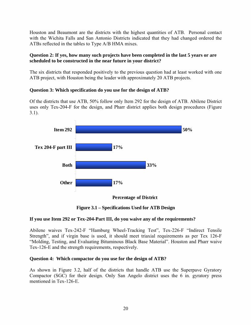
Houston and Beaumont are the districts with the highest quantities of ATB. Personal contact with the Wichita Falls and San Antonio Districts indicated that they had changed ordered the ATBs reflected in the tables to Type A/B HMA mixes. Question 2: If yes, how many such projects have been completed in the last 5 years or are scheduled to be constructed in the near future in your district? The six districts that responded positively to the previous question had at least worked with one ATB project, with Houston being the leader with approximately 20 ATB projects. Question 3: Which specification do you use for the design of ATB? Of the districts that use ATB, 50% follow only Item 292 for the design of ATB. Abilene District uses only Tex-204-F for the design, and Pharr district applies both design procedures (Figure 3.1).
Figure 3.1 – Specifications Used for ATB Design
If you use Item 292 or Tex-204-Part III, do you waive any of the requirements? Abilene waives Tex-242-F “Hamburg Wheel-Tracking Test”, Tex-226-F “Indirect Tensile Strength”, and if virgin base is used, it should meet triaxial requirements as per Tex 126-F “Molding, Testing, and Evaluating Bituminous Black Base Material”. Houston and Pharr waive Tex-126-E and the strength requirements, respectively. Question 4: Which compactor do you use for the design of ATB? As shown in Figure 3.2, half of the districts that handle ATB use the Superpave Gyratory Compactor (SGC) for their design. Only San Angelo district uses the 6 in. gyratory press mentioned in Tex-126-E.
50%
17%
33%
17%
Item 292
Tex 204-F part III
Both
Other
Percentage of District

21
Figure 3.2 – Compactors used for ATB design
Question 5: What are the main uses of ATB in your district? Most of the districts make use of ATB as an alternative to stabilized base and to Type A/B HMA (Figure 3.3.). Pharr District also applies ATB to reduce the pavement structure by eliminating the lime-treated subgrade at high volume intersection.
Figure 3.3 - Main Uses of ATB
33%
50%
0%
17%
TGC
SGC
Both
Other
Percentage of District
33%
67%
67%
0%
17%
Alternative to unbound base
Alternative to stabilized base
Alternative to Type A/B HMA
Alternative to bond breaker under PCC
Other
Percentage of District
22
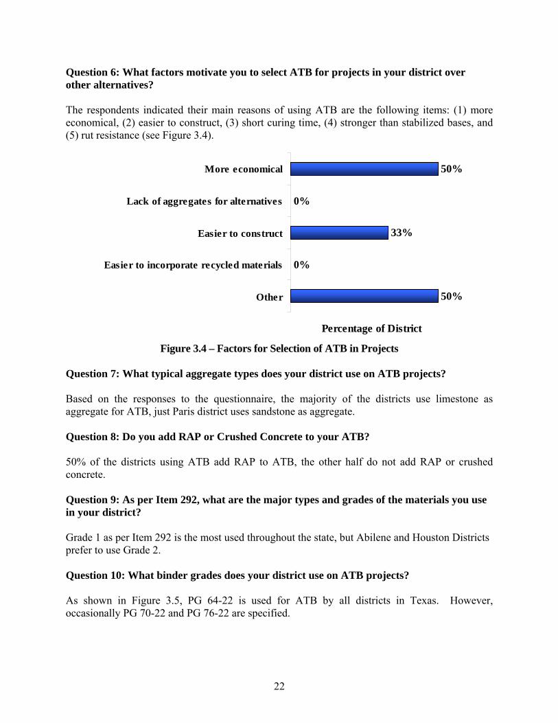
Question 6: What factors motivate you to select ATB for projects in your district over other alternatives? The respondents indicated their main reasons of using ATB are the following items: (1) more economical, (2) easier to construct, (3) short curing time, (4) stronger than stabilized bases, and (5) rut resistance (see Figure 3.4).
Figure 3.4 – Factors for Selection of ATB in Projects
Question 7: What typical aggregate types does your district use on ATB projects? Based on the responses to the questionnaire, the majority of the districts use limestone as aggregate for ATB, just Paris district uses sandstone as aggregate. Question 8: Do you add RAP or Crushed Concrete to your ATB? 50% of the districts using ATB add RAP to ATB, the other half do not add RAP or crushed concrete. Question 9: As per Item 292, what are the major types and grades of the materials you use in your district? Grade 1 as per Item 292 is the most used throughout the state, but Abilene and Houston Districts prefer to use Grade 2. Question 10: What binder grades does your district use on ATB projects? As shown in Figure 3.5, PG 64-22 is used for ATB by all districts in Texas. However, occasionally PG 70-22 and PG 76-22 are specified.
50%
0%
33%
0%
50%
More economical
Lack of aggregates for alternatives
Easier to construct
Easier to incorporate recycled materials
Other
Percentage of District

23
Figure 3.5 – Binder used for ATB projects
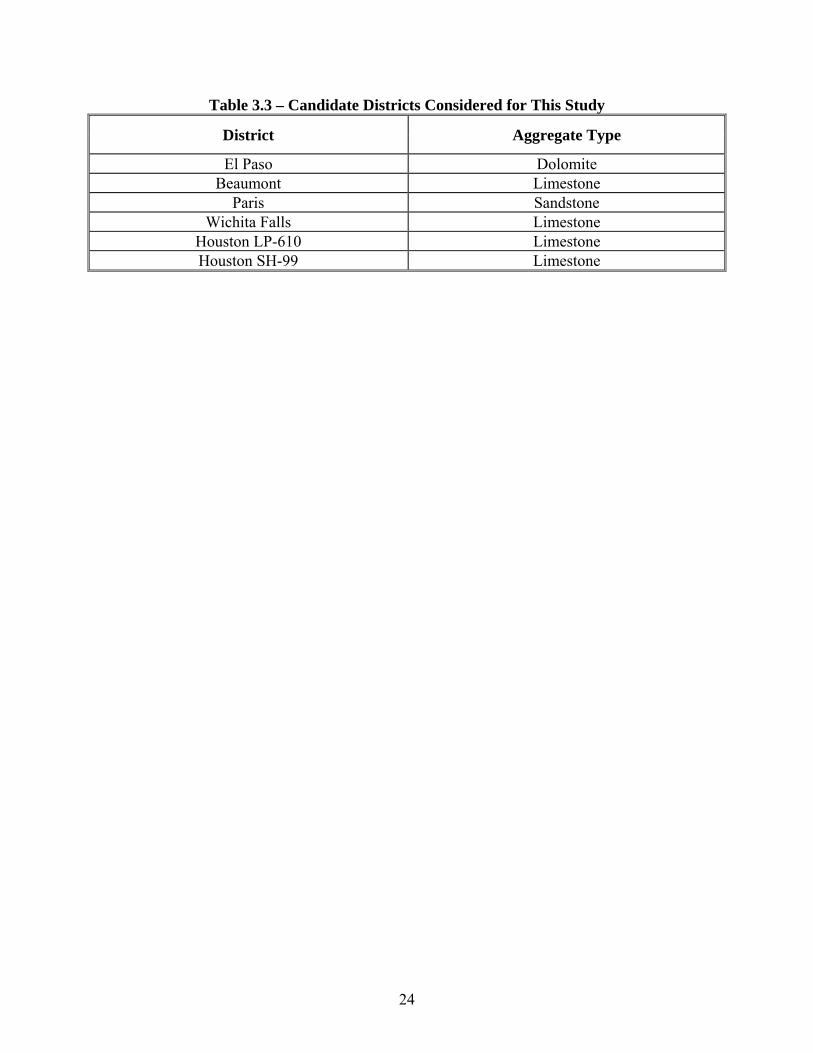
Question 11: What criteria are used to determine the amounts of binder? Most of the districts that responded positively to the use of ATB in projects determine the amount of binder following TxDOT specifications, mainly density. San Angelo district bases the amount of binder on Area Engineer’s preference and experience. Question 12: What construction specifications do you use for your projects? Half of the districts follow Item 292 for construction purposes. Pharr District states a lift thickness no greater than 4 in. Paris District requires 5% to 9% air voids calculated by the Theoretical Maximum Specific Gravity. Question 13: What types of problems, if any, have you encountered with design or construction of ATB? Based on the questionnaire, the districts were satisfied with the performance of their projects. However, segregation is mentioned as a more frequent problem presented in ATB than in HMA. The Houston and Paris Districts staff was visited to obtain insight in their use of ATB, their current mix design processes and their concerns. The insight gained by the research staff from these two districts was quite evaluable. Based on the questionnaire and interaction with the PMC, the candidate districts that were considered for this study are shown in Table 3.3.
100%
33%
17%
PG 64-22
PG 70-22
PG 76-22
Percentage of District
24
Table 3.3 – Candidate Districts Considered for This Study
District Aggregate Type
El Paso Dolomite Beaumont Limestone
Paris Sandstone Wichita Falls Limestone
Houston LP-610 Limestone Houston SH-99 Limestone
25
CHAPTER FOUR – COMPREHENSIVE EVALUATION OF ALTERNATIVE PROTOCOLS The current methods commonly used by the districts were described in Chapter 2. This section contain an explanation of those methods along with two alternative proposed methods that are more in line with the operational requirements of TxDOT. Table 4.1 shows a summary of the different mix design methods used in this study. The main differences between mix design methods are; how the optimum asphalt content (OAC) is calculated, the size of the specimens, curing temperature and the strength test. To set the criteria for each method and to select a preferred method, a comparative study of the properties of different mixes was carried out.
Table 4.1 – Summary of Mix Design Methods Baseline Mix Design Tex-126-E Tex-204-F Tex-126-H Tex-204-H
Compactor TGBC SGC SGC SGC Specimen Size, in. 6x8 6x4.5 6x8 6x4.5
OAC based on Asphalt
Density Curve Volumetric Properties
Asphalt Density Curve
Asphalt Density Curve
Curing and Testing Temperature, °F
140 77 140 77
Strength Test UCS IDT UCS IDT
Tex-126-E In this method, ATBs are molded using a Texas Gyratory Base Compactor (TGBC). Several specimens with different asphalt contents are prepared and tested to develop an asphalt content-density curve and an asphalt content-unconfined compressive strength (UCS) curve. The OAC is determined from the asphalt content-density curve. The ATB specimens are made in duplicates and are tested for their unconfined compressive strengths at 140°F. The specimens are subjected to two types of deformation rates: slow (0.15 in./min) and fast (10 in./min.) Specimens tested at a slow deformation rate yield relatively lower UCS’s as compared to the fast deformation rate ones. From the UCS-density relationship, the minimum density that would satisfy the UCS requirements as per Item 292 is taken as the minimum allowable density.
Tex-204-F This procedure was originally developed to design Type A and Type B hot mix at 97% density using 6 in. x 4½ in. specimens. Unless otherwise indicated, the specimens are molded to 100

26
gyrations using a SGC. The quality of the mix assessed with the indirect tensile strength at a deformation rate of 2 in./min and a nominal temperature of 77oF.
Proposed Tex-126-H The proposed Tex-126-H (hybrid) is similar to Tex-126-E, with one exception. While Tex-126-E uses a Texas Gyratory Base Compactor (TGBC), Tex-126-H advocates the use of a Superpave Gyratory Compactor (SGC) to produce the specimens. The other aspects of the protocol are the same as Tex-126-E, where the asphalt-density curve and UCS-density curve are developed to assess the OAC and field density.
Proposed Tex-204-H The second proposed method, Tex-204-H (Hybrid), is similar to Tex-204-F. The only difference is the way the OAC is selected. For Tex-204-H, the requirements for volumetric properties such as VFA are waived because it is not possible to modify the gradation to achieve the required volumetric properties. In Tex-204-H protocol, attention is paid to asphalt-density curve, similar to Tex-126-H, and the IDT strength.
Comparison of Properties from Different Approaches Mix designs were performed on six materials (see Table 3.3) following the four approaches indicated above to highlight their similarities and differences. To demonstrate different approaches a local material from El Paso is used as an example. Results from the other materials are then summarized.
Index Properties The gradation curves of all materials as received are shown in Figure 4.1. To prepare the materials for mix design, the entire stock of the material was sieved first to develop a global gradation curve. This gradation curve was used throughout the study. The acceptable range as per Item 292 Grade 1 is also shown in the figure. Houston SH-99 and Paris materials do not fulfill those requirements. Figure 4.2 illustrates the material constituents for all materials. Houston SH-99 and Paris have higher concentrations of gravel (72% and 70%, respectively) while El Paso material has the lowest gravel concentration (55%). Coarse sand contents range from 9% to 28%, with Houston SH-99 containing the lowest concentration and Wichita Falls the highest. The fine sand contents of all materials are similar, ranging from 12% to 18%. El Paso and Wichita Falls have the highest fines concentrations (5%) while other materials contain 1% to 2% fines. Material classifications as per Unified Soil Classification System (USCS) and American Association of State Highway and Transportation Officials (AASHTO) Soil Classification System, as well as the Atterberg limits are summarized in Table 4.2. Under the USCS, all materials classified as GP (poorly-graded gravel) except for Houston LP-610 and Wichita Falls which were categorized as GW (well-graded gravel). All materials are classified as A-1-a under the AASHTO system. All materials seem to be non-plastic except Wichita Falls.

1P
erce
nt
Pas
sin
g1
Per
cen
t P
assi
ng
1P
erce
nt
Pas
sin
g
Figure 4.1 –
Figu
0
10
20
30
40
50
60
70
80
90
100
100
G
0
10
20
30
40
50
60
70
80
90
100
100
G
0
10
20
30
40
50
60
70
80
90
100
100
G
– Gradation
ure 4.2 – Ma
10
Gravel
10
Gravel
10
Gravel
n Curves fro
aterial Cons
#4#4#4
27
om Different
stituents for
1Sieve size, mm
#4
Sand
1Sieve size, mm
#4
Sand
1Sieve size, mm
#4
Sand
t Materials U
the Sites Be
0.m
40
0.m
40
0.m
40
Used in Thi
eing Studied
1
El Paso
Beaumo
Houston
Houston
Paris
Wichita
Item 29
#200
Fines
1
El Paso
Beaumo
Houston
Houston
Paris
Wichita
Item 29
#200
Fines
1
El Paso
Beaumo
Houston
Houston
Paris
Wichita
Item 29
#200
Fines
is Study
d
0.01
ont
n SH-99
n I-60
a Falls
2
LP-610
0.01
ont
n SH-99
n I-60
a Falls
2
0.01
ont
n SH-99
n I-60
a Falls
2
LP-610
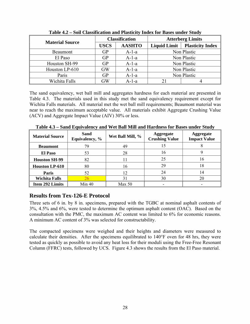
28
Table 4.2 – Soil Classification and Plasticity Index for Bases under Study
Material Source Classification Atterberg Limits
USCS AASHTO Liquid Limit Plasticity Index Beaumont GP A-1-a Non Plastic
El Paso GP A-1-a Non Plastic Houston SH-99 GP A-1-a Non Plastic Houston LP-610 GW A-1-a Non Plastic
Paris GP A-1-a Non Plastic Wichita Falls GW A-1-a 21 4
The sand equivalency, wet ball mill and aggregates hardness for each material are presented in Table 4.3. The materials used in this study met the sand equivalency requirement except for Wichita Falls materials. All material met the wet ball mill requirements; Beaumont material was near to reach the maximum acceptable value. All materials exhibit Aggregate Crushing Value (ACV) and Aggregate Impact Value (AIV) 30% or less.
Table 4.3 – Sand Equivalency and Wet Ball Mill and Hardness for Bases under Study
Material Source Sand Equivalency, % Wet Ball Mill, % Aggregate
Crushing Value Aggregate
Impact Value
Beaumont 79 49 15 8
El Paso 53 28 16 9
Houston SH-99 82 11 25 16
Houston LP-610 80 16 29 18
Paris 52 12 24 14 Wichita Falls 26 31 30 20
Item 292 Limits Min 40 Max 50 - -
Results from Tex-126-E Protocol Three sets of 6 in. by 8 in. specimens, prepared with the TGBC at nominal asphalt contents of 3%, 4.5% and 6%, were tested to determine the optimum asphalt content (OAC). Based on the consultation with the PMC, the maximum AC content was limited to 6% for economic reasons. A minimum AC content of 3% was selected for constructability. The compacted specimens were weighed and their heights and diameters were measured to calculate their densities. After the specimens equilibrated to 140°F oven for 48 hrs, they were tested as quickly as possible to avoid any heat loss for their moduli using the Free-Free Resonant Column (FFRC) tests, followed by UCS. Figure 4.3 shows the results from the El Paso material.
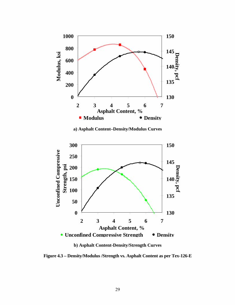
29
a) Asphalt Content–Density/Modulus Curves
b) Asphalt Content-Density/Strength Curves
Figure 4.3 – Density/Modulus /Strength vs. Asphalt Content as per Tex-126-E
0
200
400
600
800
1000
2 3 4 5 6 7Asphalt Content, %
Mod
ulus
, ksi
130
135
140
145
150
Density, pcf
Modulus Density
0
50
100
150
200
250
300
2 3 4 5 6 7Asphalt Content, %
Unc
onfi
ned
Com
pres
sive
Stre
ngth
, psi
130
135
140
145
150
Density, pcf
Unconfined Compressive Strength Density
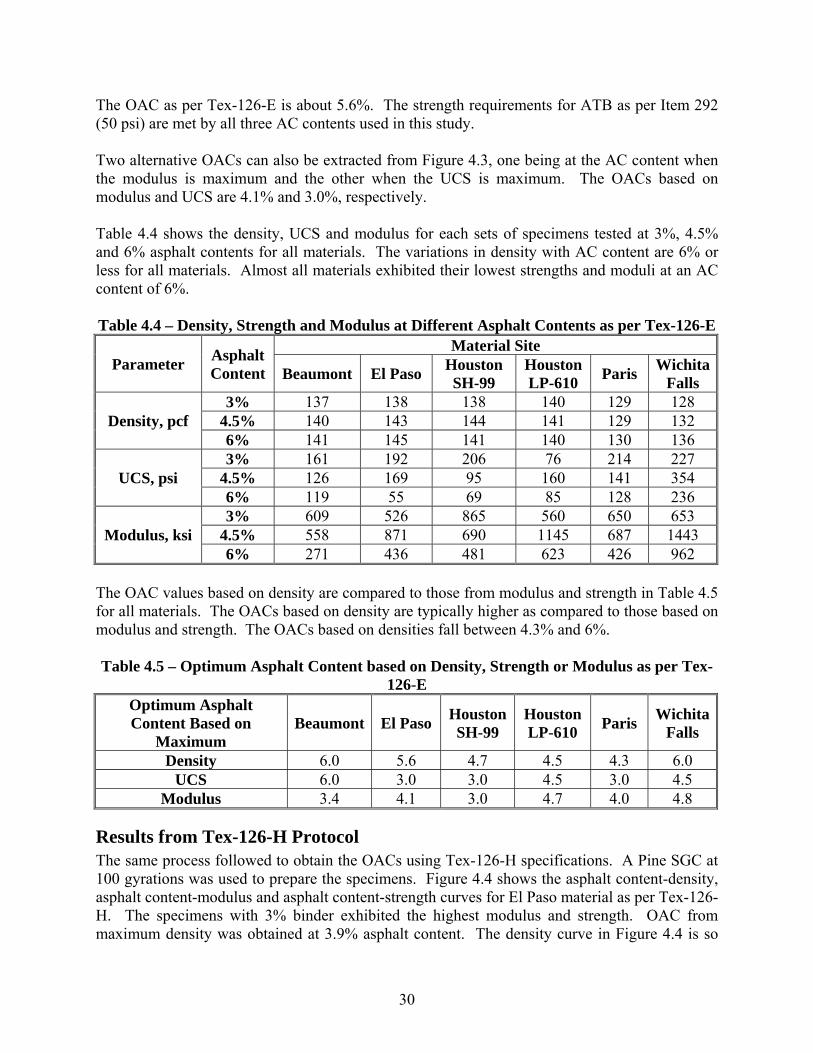
30
The OAC as per Tex-126-E is about 5.6%. The strength requirements for ATB as per Item 292 (50 psi) are met by all three AC contents used in this study. Two alternative OACs can also be extracted from Figure 4.3, one being at the AC content when the modulus is maximum and the other when the UCS is maximum. The OACs based on modulus and UCS are 4.1% and 3.0%, respectively. Table 4.4 shows the density, UCS and modulus for each sets of specimens tested at 3%, 4.5% and 6% asphalt contents for all materials. The variations in density with AC content are 6% or less for all materials. Almost all materials exhibited their lowest strengths and moduli at an AC content of 6%. Table 4.4 – Density, Strength and Modulus at Different Asphalt Contents as per Tex-126-E
Parameter Asphalt Content
Material Site
Beaumont El Paso Houston SH-99
Houston LP-610
Paris Wichita
Falls
Density, pcf 3% 137 138 138 140 129 128
4.5% 140 143 144 141 129 132 6% 141 145 141 140 130 136
UCS, psi 3% 161 192 206 76 214 227
4.5% 126 169 95 160 141 354 6% 119 55 69 85 128 236
Modulus, ksi 3% 609 526 865 560 650 653
4.5% 558 871 690 1145 687 1443 6% 271 436 481 623 426 962
The OAC values based on density are compared to those from modulus and strength in Table 4.5 for all materials. The OACs based on density are typically higher as compared to those based on modulus and strength. The OACs based on densities fall between 4.3% and 6%.
Table 4.5 – Optimum Asphalt Content based on Density, Strength or Modulus as per Tex-
126-E Optimum Asphalt Content Based on
Maximum Beaumont El Paso
Houston SH-99
Houston LP-610
Paris Wichita
Falls
Density 6.0 5.6 4.7 4.5 4.3 6.0 UCS 6.0 3.0 3.0 4.5 3.0 4.5
Modulus 3.4 4.1 3.0 4.7 4.0 4.8
Results from Tex-126-H Protocol The same process followed to obtain the OACs using Tex-126-H specifications. A Pine SGC at 100 gyrations was used to prepare the specimens. Figure 4.4 shows the asphalt content-density, asphalt content-modulus and asphalt content-strength curves for El Paso material as per Tex-126-H. The specimens with 3% binder exhibited the highest modulus and strength. OAC from maximum density was obtained at 3.9% asphalt content. The density curve in Figure 4.4 is so
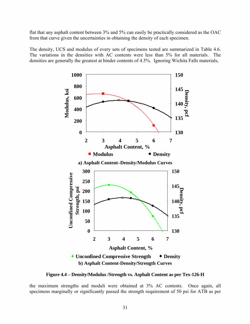
31
flat that any asphalt content between 3% and 5% can easily be practically considered as the OAC from that curve given the uncertainties in obtaining the density of each specimen. The density, UCS and modulus of every sets of specimens tested are summarized in Table 4.6. The variations in the densities with AC contents were less than 5% for all materials. The densities are generally the greatest at binder contents of 4.5%. Ignoring Wichita Falls materials,
a) Asphalt Content–Density/Modulus Curves
b) Asphalt Content-Density/Strength Curves
Figure 4.4 – Density/Modulus /Strength vs. Asphalt Content as per Tex-126-H
the maximum strengths and moduli were obtained at 3% AC contents. Once again, all specimens marginally or significantly passed the strength requirement of 50 psi for ATB as per
0
200
400
600
800
1000
2 3 4 5 6 7Asphalt Content, %
Mod
ulus
, ksi
130
135
140
145
150
Density, pcf
Modulus Density
0
50
100
150
200
250
300
2 3 4 5 6 7
Asphalt Content, %
Unc
onfi
ned
Com
pres
sive
Stre
ngth
, psi
130
135
140
145
150
Density, pcf
Unconfined Compressive Strength Density

32
Item 292. As reflected in Table 4.7, once again the highest OACs are generally obtained based on density. Table 4.6 – Density Strength and Modulus at Different Asphalt Contents as per Tex-126-H
* unable to retrieve an intact specimen after compaction and as such could not be tested. Table 4.7 – Optimum Asphalt Contents Based on Density, Strength or Modulus as per Tex-
126-H Optimum Asphalt Content Based on
Maximum Beaumont El Paso
Houston SH-99
Houston LP-610
Paris Wichita
Falls
Density 4.7 3.9 4.2 4.1 6.0 6.0 UCS 4.1 3.0 3.0 4.2 5.0 4.7
Modulus 3.6 3.0 3.4 3.0 5.5 5.4
Results from Tex-204-H Protocol The asphalt-density curve for Tex-204-H for El Paso material is illustrated in Figure 4.5. The OAC based on density is 3.9% at a density of about 139 pcf. It is hard to judge the accuracy of this OAC, since the density changes by less than 1% with the change in the asphalt content. The OACs based on modulus and IDT occur at about 5.3% and 3.7%, respectively. Since the specimens’ heights were only 4.5 in., a v-meter was used to measure the moduli. The values obtained for density, indirect tensile strength (IDT) and modulus for all materials prepared under Tex-204-H are summarized in Table 4.8. For all materials the variations in the density with asphalt content are rather small. Most materials exhibit their highest IDT strengths between asphalt contents of 3 and 4.5%. Wichita Falls specimens with 3% asphalt content could not be tested because they broke after compaction but before testing. Moduli of the specimens tested do not vary much for most materials similar to the densities. The OAC values based on maximum density, indirect tensile strength and modulus as per Tex-204-H for all materials are summarized in Table 4.9. As opposed to the Tex-126-E and Tex-126-H results, no clear pattern is apparent for this protocol.
Parameter Asphalt Content
Beaumont El Paso Houston SH-99
Houston LP-610
Paris Wichita
Falls
Density, pcf 3% 134 141 135 136 127 126
4.5% 136 141 136 137 126 130 6% 135 138 134 134 130 133
UCS, psi 3% 159 230 84 167 N/A* 207
4.5% 180 192 55 121 163 410 6% 105 73 48 70 125 301
Modulus, ksi 3% 948 664 1022 1422 N/A* 498
4.5% 960 537 915 909 527 1423 6% 462 115 369 534 600 1524
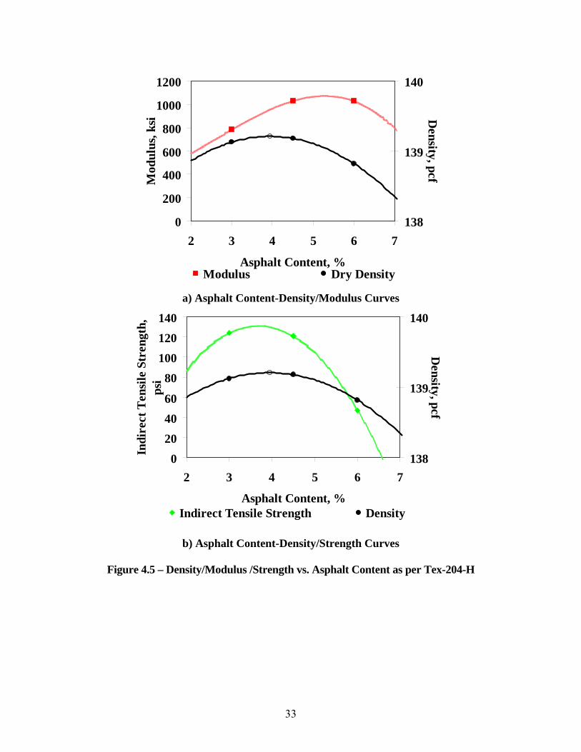
33
a) Asphalt Content-Density/Modulus Curves
b) Asphalt Content-Density/Strength Curves
Figure 4.5 – Density/Modulus /Strength vs. Asphalt Content as per Tex-204-H
0
200
400
600
800
1000
1200
2 3 4 5 6 7
Asphalt Content, %
Mod
ulus
, ksi
138
139
140
Density, pcf
Modulus Dry Density
0
20
40
60
80
100
120
140
2 3 4 5 6 7
Asphalt Content, %
Indi
rect
Ten
sile
Str
engt
h,
psi
138
139
140
Density, pcf
Indirect Tensile Strength Density
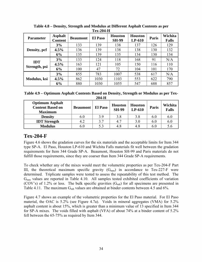
34
Table 4.8 – Density, Strength and Modulus at Different Asphalt Contents as per Tex-204-H
Parameter Asphalt Content
Beaumont El Paso Houston SH-99
Houston LP-610
Paris Wichita
Falls
Density, pcf 3% 133 139 138 137 126 129
4.5% 136 139 138 138 130 132 6% 135 139 135 134 130 134
IDT Strength, psi
3% 133 124 118 168 91 N/A 4.5% 163 121 105 150 116 110 6% 100 47 72 104 101 170
Modulus, ksi 3% 855 783 1007 538 617 N/A
4.5% 862 1030 1103 553 622 790 6% 880 1030 1055 547 688 857
Table 4.9 – Optimum Asphalt Contents Based on Density, Strength or Modulus as per Tex-
204-H Optimum Asphalt Content Based on
Maximum Beaumont El Paso
Houston SH-99
Houston LP-610
Paris Wichita
Falls
Density 6.0 3.9 3.8 3.8 6.0 6.0 IDT Strength 4.2 3.7 4.7 3.0 6.0 6.0
Modulus 6.0 5.3 4.8 4.8 6.0 5.6
Tex-204-F Figure 4.6 shows the gradation curves for the six materials and the acceptable limits for Item 344 type SP-A. El Paso, Houston LP-610 and Wichita Falls materials fit well between the gradation requirements for Item 344 Grade SP-A. Beaumont, Houston SH-99 and Paris materials do not fulfill those requirements, since they are coarser than Item 344 Grade SP-A requirements. To check whether any of the mixes would meet the volumetric properties as per Tex-204-F Part III, the theoretical maximum specific gravity (Gmm) in accordance to Tex-227-F were determined. Triplicate samples were tested to assess the repeatability of this test method. The Gmm values are reported in Table 4.10. All samples tested exhibited coefficients of variation (COV’s) of 1.2% or less. The bulk specific gravities (Gmb) for all specimens are presented in Table 4.11. The maximum Gmb values are obtained at binder contents between 4.5 and 6%. Figure 4.7 shows an example of the volumetric properties for the El Paso material. For El Paso material, the OAC is 5.2% (see Figure 4.7a). Voids in mineral aggregates (VMA) for 5.2% asphalt content is about 15%, which is greater than a minimum value of 13 specified in Item 344 for SP-A mixes. The voids filled with asphalt (VFA) of about 74% at a binder content of 5.2% fell between the 65-75% as required by Item 344.
35
Figure 4.6 – Gradation Curves from Different Materials Compared to
Item 344 Grade SP-A
Table 4.10 – Maximum Theoretical Specific Gravities for Tex-204-H Specimens Asphalt Content
Parameter Beaumont El Paso Houston SH-99
Houston LP-610
Paris Wichita
Falls
3.0% Average 2.45 2.62 2.51 2.47 2.37 2.55 COV* 0.3% 0.5% 0.3% 0.4% 0.1% 0.4%
4.5% Average 2.45 2.55 2.43 2.41 2.46 2.48
COV 0.2% 0.7% 0.1% 0.1% 0.3% 0.1%
6.0% Average 2.39 2.46 2.38 2.36 2.4 2.41
COV 0.3% 1.2% 0.4% 0.2% 0.7% 1.1% * COV = coefficient of variation
Table 4.11 – Bulk Specific Gravities for Tex-204-H Specimens Asphalt Content
Beaumont El Paso Houston SH-99
Houston LP-610
Paris Wichita
Falls 3.0% 2.33 2.41 2.39 2.30 2.25 2.28
4.5% 2.37 2.47 2.40 2.35 2.30 2.37
6.0% 2.41 2.40 2.41 2.30 2.34 2.41
0
10
20
30
40
50
60
70
80
90
100
0.010.1110100Sieve size, mm
Per
cen
t P
assi
ng
El Paso
Beaumont
Houston SH-99
Houston I-60
Paris
Wichita Falls
344 SP-A
#4 #40 #200
Gravel Sand Fines
LP-610

36
Figure 4.7 – Volumetric Properties for El Paso Material Table 4.12 shows the volumetric properties for all specimens as well as the requirements to be met for Item 344 SP-A mixes. The majority of the materials successfully passed the requirements, except for the VFA value for Houston SH-99, Paris and Wichita Falls.
Table 4.12 – Volumetric Properties for Tex-204-H Specimens
Values at 4% Air Voids
Beaumont El Paso Houston SH-99
Houston LP-610
Paris Wichita
Falls
Item 344 Grade SP-A
AC, % 4.0 5.2 3.7 4.3 5.8 5.0 -
VMA, % 14.3 14.9 20.2 14.8 18.4 15.6 Min. 13
VFA, % 71.5 74.1 80.4 72.4 78 75.5 65-75
Moisture Susceptibility One of the test methods used to quantify moisture susceptibility is Tex-242-F, Hamburg Wheel-Tracking Test (HWTD). This test was performed on specimens prepared at OAC’s determined from Tex-126-H and Tex-204-H protocols based on density. The results for the HWTD are summarized in Table 4.13. Even though the minimum number of passes required for a PG 64-22 binder is 10,000, tests were continued up to 20,000 passes. All specimens tested exhibited acceptable rut depths at 10,000 cycles. All specimens were in the acceptable limits at 15,000 and
y = -2.0x + 14.4
R2 = 0.9
0123456789
10
2.5 3.0 3.5 4.0 4.5 5.0 5.5 6.0 6.5Asphalt Content, %
Air
Voi
ds, %
a
a)
y = -2.0x + 14.4
R2 = 0.9
0123456789
10
2.5 3.0 3.5 4.0 4.5 5.0 5.5 6.0 6.5Asphalt Content, %
Air
Voi
ds, %
a y = -2.0x + 14.4
R2 = 0.9
0123456789
10
2.5 3.0 3.5 4.0 4.5 5.0 5.5 6.0 6.5Asphalt Content, %
Air
Voi
ds, %
a
a)y = 0.9x2 - 6.9x + 27.6
R2 = 1.0101112131415161718
2.5 3.5 4.5 5.5 6.5Asphalt Content, %
VM
A, %
b
b) y = 0.9x2 - 6.9x + 27.6
R2 = 1.0101112131415161718
2.5 3.5 4.5 5.5 6.5Asphalt Content, %
VM
A, %
b
y = 0.9x2 - 6.9x + 27.6
R2 = 1.0101112131415161718
2.5 3.5 4.5 5.5 6.5Asphalt Content, %
VM
A, %
b
b)
y = 14.6x - 1.9
R2 = 1.030
40
50
60
70
80
90
2.5 3.5 4.5 5.5 6.5
Asphalt Content, %
VF
A, %
c
c)
y = 14.6x - 1.9
R2 = 1.030
40
50
60
70
80
90
2.5 3.5 4.5 5.5 6.5
Asphalt Content, %
VF
A, %
c
y = 14.6x - 1.9
R2 = 1.030
40
50
60
70
80
90
2.5 3.5 4.5 5.5 6.5
Asphalt Content, %
VF
A, %
c
c)
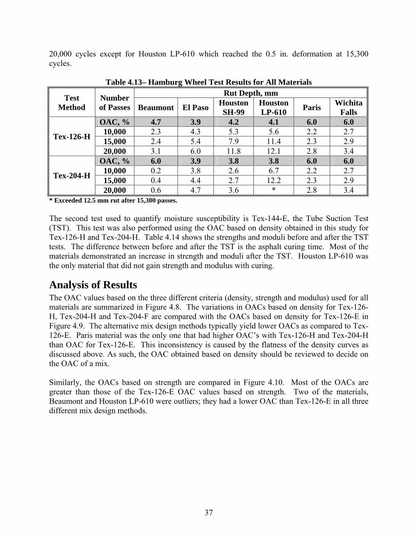
37
20,000 cycles except for Houston LP-610 which reached the 0.5 in. deformation at 15,300 cycles.
Table 4.13– Hamburg Wheel Test Results for All Materials
Test Method
Number of Passes
Rut Depth, mm
Beaumont El Paso Houston SH-99
Houston LP-610
Paris Wichita
Falls
Tex-126-H
OAC, % 4.7 3.9 4.2 4.1 6.0 6.0 10,000 2.3 4.3 5.3 5.6 2.2 2.7 15,000 2.4 5.4 7.9 11.4 2.3 2.9 20,000 3.1 6.0 11.8 12.1 2.8 3.4
Tex-204-H
OAC, % 6.0 3.9 3.8 3.8 6.0 6.0 10,000 0.2 3.8 2.6 6.7 2.2 2.7 15,000 0.4 4.4 2.7 12.2 2.3 2.9 20,000 0.6 4.7 3.6 * 2.8 3.4
* Exceeded 12.5 mm rut after 15,300 passes. The second test used to quantify moisture susceptibility is Tex-144-E, the Tube Suction Test (TST). This test was also performed using the OAC based on density obtained in this study for Tex-126-H and Tex-204-H. Table 4.14 shows the strengths and moduli before and after the TST tests. The difference between before and after the TST is the asphalt curing time. Most of the materials demonstrated an increase in strength and moduli after the TST. Houston LP-610 was the only material that did not gain strength and modulus with curing.
Analysis of Results The OAC values based on the three different criteria (density, strength and modulus) used for all materials are summarized in Figure 4.8. The variations in OACs based on density for Tex-126-H, Tex-204-H and Tex-204-F are compared with the OACs based on density for Tex-126-E in Figure 4.9. The alternative mix design methods typically yield lower OACs as compared to Tex-126-E. Paris material was the only one that had higher OAC’s with Tex-126-H and Tex-204-H than OAC for Tex-126-E. This inconsistency is caused by the flatness of the density curves as discussed above. As such, the OAC obtained based on density should be reviewed to decide on the OAC of a mix. Similarly, the OACs based on strength are compared in Figure 4.10. Most of the OACs are greater than those of the Tex-126-E OAC values based on strength. Two of the materials, Beaumont and Houston LP-610 were outliers; they had a lower OAC than Tex-126-E in all three different mix design methods.

38
Table 4.14 – Impact of Tube Suction Tests on UCS and Seismic Modulus
Test Method
Parameter Beaumont El Paso
Houston SH-99
Houston LP-610
Paris Wichita Falls
Before After Before After Before After Before After Before After Before After
Tex
-126
-H OAC, % 4.7 3.9 4.2 4.1 6.0 6.0
UCS, psi 405 509 485 653 373 498 583 539 337 446 392 426
Modulus, ksi
2411 2242 1739 3028 1279 2738 2494 2462 1720 2482 1940 2054
Tex
-204
-H OAC, % 6.0 3.9 3.8 3.8 6.0 6.0
IDTS, psi 92 107 123 190 63 148 203 153 98 134 143 212
Modulus, ksi
833 938 825 901 835 1123 910 834 872 919 882 834
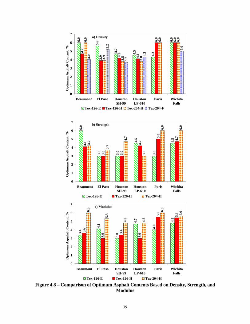
39
Figure 4.8 – Comparison of Optimum Asphalt Contents Based on Density, Strength, and
Modulus
6.0
5.6
4.7
4.5
4.3
6.0
4.7
3.9 4.
2
4.1
6.0
6.0
6.0
3.9
3.8
3.8
6.0
6.0
4.0
5.2
3.7
4.3
5.0
0
1
2
3
4
5
6
7
Beaumont El Paso HoustonSH-99
HoustonLP-610
Paris WichitaFalls
Op
tim
um
Asp
hal
t C
onte
nt,
%
Tex-126-E Tex-126-H Tex-204-H Tex-204-F
a) Density
6.0
3.0
3.0
4.5
3.0
4.5
4.1
3.0
3.0
4.2
5.0
4.7
4.2
3.7
4.7
3.0
6.0
6.0
0
1
2
3
4
5
6
7
Beaumont El Paso HoustonSH-99
HoustonLP-610
Paris WichitaFalls
Op
tim
um
Asp
hal
t C
onte
nt,
%
.
Tex-126-E Tex-126-H Tex-204-H
b) Strength
3.4
4.1
3.0
4.7
4.0
4.8
3.6
3.0 3.
4
3.0
5.5
5.4
6.0
5.3
4.8
4.8
6.0
5.6
0
1
2
3
4
5
6
7
Beaumont El Paso HoustonSH-99
HoustonLP-610
Paris WichitaFalls
Op
tim
um
Asp
ahal
t C
onte
nt,
%
.
Tex-126-E Tex-126-H Tex-204-H
c) Modulus
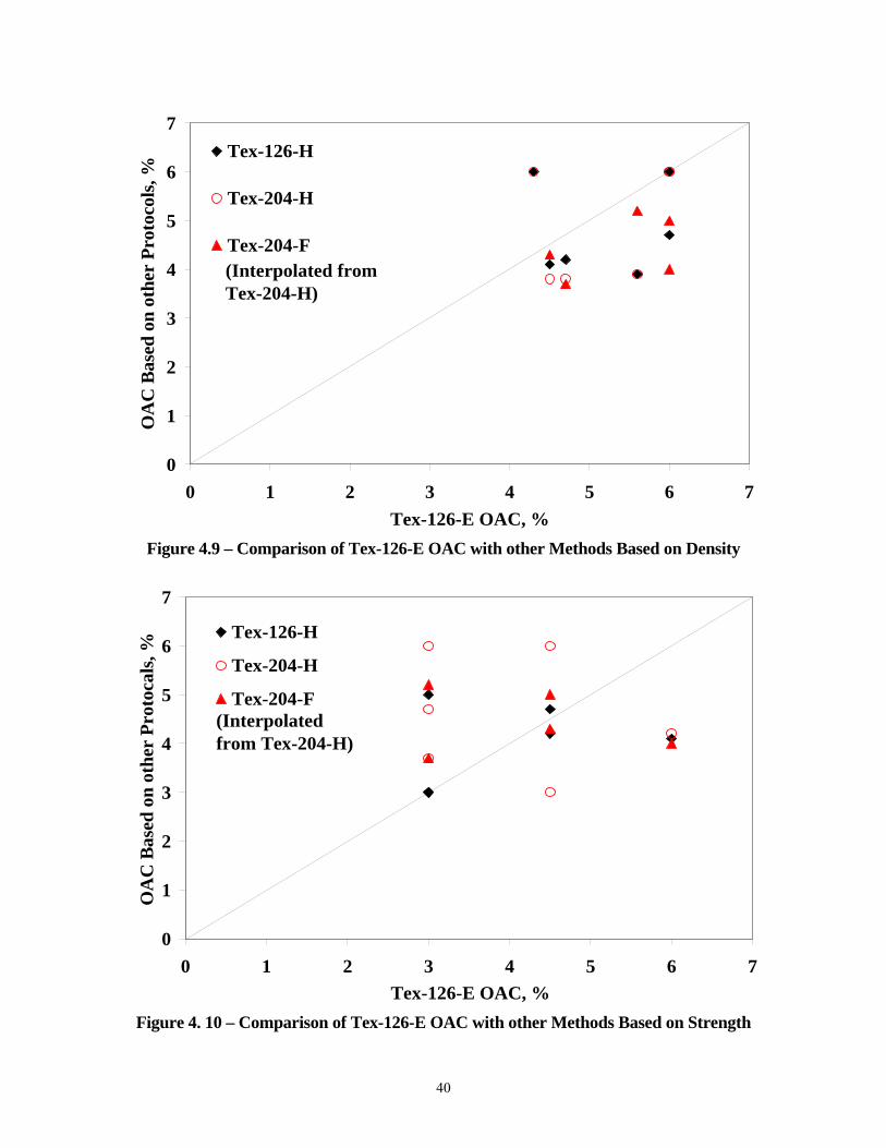
40
Figure 4.9 – Comparison of Tex-126-E OAC with other Methods Based on Density
Figure 4. 10 – Comparison of Tex-126-E OAC with other Methods Based on Strength
0
1
2
3
4
5
6
7
0 1 2 3 4 5 6 7
Tex-126-E OAC, %
OA
C B
ased
on
oth
er P
roto
cols
, %Tex-126-H
Tex-204-H
Tex-204-F(Interpolated from Tex-204-H)
0
1
2
3
4
5
6
7
0 1 2 3 4 5 6 7
Tex-126-E OAC, %
OA
C B
ased
on
oth
er P
roto
cals
, % Tex-126-H
Tex-204-H
Tex-204-F(Interpolated from Tex-204-H)
41
The OAC values based on modulus are compared in Figure 4.11. Similarly most of the OACs are greater than that of Tex-126-E values based on modulus with three outliers Houston LP-610 (Tex-126-H and Tex-204-F) and El Paso (Tex-126-H). Figure 4.12 shows the maximum densities for all materials and for all mix design methods. For a given mix, the densities are fairly close. The maximum density for most materials is generally reached when Tex-126-E is followed. The lowest densities are typically obtained from Tex-204-F by waiving some of the volumetric requirements. For comparison purposes, UCS and IDT specimens were prepared based on OAC of each method and were tested for strength and modulus. The variations in the UCS values are shown in Figure 4.13. All materials reached the 50 psi strength requirement for ATB as per Item 292. The strongest material is Wichita Falls while the weakest material analyzed was Houston SH-99. The specimens prepared with the Superpave Gyratory Compactor usually exhibit similar or higher UCS as compared to those prepared with the Texas Gyratory Compactor. The IDT strengths obtained from 6 x 4.5 in. specimens are shown in Figure 4.14. No obvious pattern could be found in the data. Given the uncertainty in the IDT tests, in most cases the strengths are similar from different methods of estimating OAC. Finally, the moduli obtained from these specimens are shown in Figures 4.15 and 4.16. The variations in moduli are in line with the corresponding strengths shown in Figures 4.13 and 4.14. So far this study shows that mix design using the SGC is feasible. Based on the results reported in this chapter, the adoption of either Tex-126-H or Tex-204-H will be discussed.

42
Figure 4.11 – Comparison of Tex-126-E OAC with other Methods Based on Modulus
*-Values are interpolated
Figure 4.12 – Densities at OACs for Each Test Method
0
1
2
3
4
5
6
7
0 1 2 3 4 5 6 7
Tex-126-E OAC, %
OA
C B
ased
on
oth
er P
roto
cols
, %Tex-126-H
Tex-204-H
Tex-204-F
(Interpolated from Tex-204-H)
141
145
144
141
129
13613
7
141
136 13
8
129
133
137 13
9
138 13
9
130
13413
6
139
136 13
8
133
120
125
130
135
140
145
150
Beaumont El Paso Houston SH-99
Houston LP-610
Paris Wichita Falls
Den
sity
, pcf
Tex-126-E Tex-126-H Tex-204-H Tex-204-F*
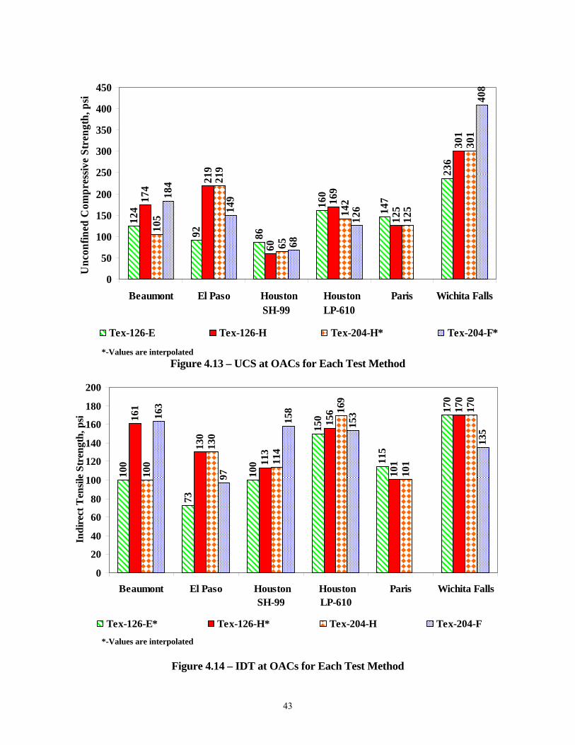
43
*-Values are interpolated
Figure 4.13 – UCS at OACs for Each Test Method
*-Values are interpolated
Figure 4.14 – IDT at OACs for Each Test Method
124
92 86
160
147
236
174
219
60
169
125
301
105
219
65
142
125
301
184
149
68
126
408
0
50
100
150
200
250
300
350
400
450
Beaumont El Paso Houston SH-99
Houston LP-610
Paris Wichita Falls
Un
con
fin
ed C
omp
ress
ive
Str
engt
h, p
si .
Tex-126-E Tex-126-H Tex-204-H* Tex-204-F*
100
73
100
150
115
170
161
130
113
156
101
170
100
130
114
169
101
170
163
97
158
153
135
0
20
40
60
80
100
120
140
160
180
200
Beaumont El Paso Houston SH-99
Houston LP-610
Paris Wichita Falls
Ind
irec
t T
ensi
le S
tren
gth
, psi
Tex-126-E* Tex-126-H* Tex-204-H Tex-204-F
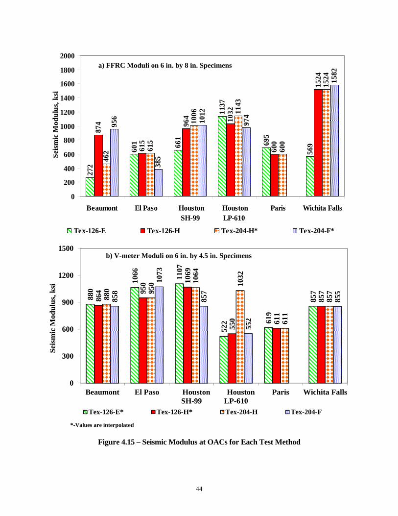
44
*-Values are interpolated
Figure 4.15 – Seismic Modulus at OACs for Each Test Method
272
601 66
1
1137
695
569
874
615
964 10
32
600
1524
462 61
5
1006 11
43
600
1524
956
385
1012
974
1582
0
200
400
600
800
1000
1200
1400
1600
1800
2000
Beaumont El Paso Houston SH-99
Houston LP-610
Paris Wichita Falls
Sei
smic
Mod
ulu
s, k
si
Tex-126-E Tex-126-H Tex-204-H* Tex-204-F*
a) FFRC Moduli on 6 in. by 8 in. Specimens
880
1066 1107
522 61
9
857
864 95
0 1069
550 61
1
857
880 95
0 1064
1032
611
857
858
1073
857
552
855
0
300
600
900
1200
1500
Beaumont El Paso HoustonSH-99
HoustonLP-610
Paris Wichita Falls
Sei
smic
Mod
ulu
s, k
si
Tex-126-E* Tex-126-H* Tex-204-H Tex-204-F
b) V-meter Moduli on 6 in. by 4.5 in. Specimens

45
CHAPTER FIVE – EVALUATION OF PARAMETERS THAT IMPACT PERFORMANCE The two alternative protocols deemed reasonable for fulfilling the objectives of this project are Tex-126-H and Tex-204-H. Many specimens were mixed, compacted and tested at different numbers of gyrations using the SGC to evaluate the impact of the number of gyrations on the properties of the mixes. Specimens were also mixed and compacted using the TGBC to try to match the densities of the SGC specimens with the ones compacted using the TGBC. The impact of curing temperature is also presented in this chapter in which specimens were tested after 24 or 48 hrs of curing at 77°F or 140°F. Two different grades of asphalt (PG 76-22 and PG 64-22) were evaluated as well. The differences in optimum asphalt content, density, strength and modulus between the two binders are presented. The impact of the change in gradation on optimum asphalt content, density, strength and modulus is summarized at the end of this chapter.
Impact of Number of Gyrations
Tex-126-H Protocol The impact of the number of gyrations on the (OAC based on density as per Tex-126-H is summarized in Figure 5.1. The OAC’s for Paris and Wichita Falls seem to be 6% (upper limit imposed on the asphalt content) or greater. Except for the Houston SH-99, the increase in the number of gyrations results in typically less than 1% change in the OAC. The OAC’s as per Tex-126-E are also included in Figure 5.1. The OAC’s for 60 to 80 gyrations are typically closer to the OAC’s from Tex-126-E. The densities at corresponding OAC’s for different numbers of gyrations of SGC are compared with those from Tex-126-E in Figure 5.2. The impact of the number of gyrations of SGC on density is rather small (typically less than 3 pcf). In almost all cases, the highest densities are associated with Tex-126-E protocol. The impact of the number of gyrations on UCS and modulus are shown in Figures 5.3 and 5.4, respectively. All specimens were prepared to the nominal dimensions of 6 in. by 8 in. The UCS and modulus values mostly follow the same pattern. As the UCS increases the modulus also increases. A clear pattern is not evident in these results primarily because of the complex interaction of the compaction energy with the asphalt content. The other complicating factor is the so-called locking point during the compaction with the SGC. Locking point is defined as the
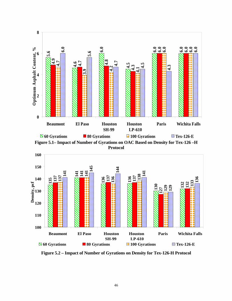
46
Figure 5.1– Impact of Number of Gyrations on OAC Based on Density for Tex-126 –H
Protocol
Figure 5.2 – Impact of Number of Gyrations on Density for Tex-126-H Protocol
5.6
4.6
6.0
4.5
6.0
6.0
4.9
4.7 4.8
4.3
6.0
6.0
4.7
3.9 4.
2
4.1
6.0
6.0
6.0
5.6
4.7
4.5
4.3
6.0
0
2
4
6
8
Beaumont El Paso Houston SH-99
Houston LP-610
Paris Wichita Falls
Opt
imum
Asp
halt
Con
tent
, %
60 Gyrations 80 Gyrations 100 Gyrations Tex-126-E
135
141
136
136
130 13213
7 141
137
137
127 13
2137 14
1
136 13
8
129 13
3
141 14
5
144
141
129
136
100
110
120
130
140
150
160
Beaumont El Paso Houston SH-99
Houston LP-610
Paris Wichita Falls
Den
sity
, pcf
60 Gyrations 80 Gyrations 100 Gyrations Tex-126-E

47
Figure 5.3 – Impact of Number of Gyrations on UCS for Tex-126-H Protocol
Figure 5.4 – Impact of Number of Gyrations on Modulus for Tex-126-H Protocol
210
204
67
93 100
301
169
208
69
134
133
311
174
219
60
169
125
301
124
92 86
160
147
236
0
50
100
150
200
250
300
350
Beaumont El Paso Houston SH-99
Houston LP-610
Paris Wichita Falls
Unc
onfi
ned
Com
pres
sive
Str
engt
h, p
si
60 Gyrations 80 Gyrations 100 Gyrations Tex-126-E
817
419
567
788
373
1117
720
640 71
0
1130
512
1158
874
615
964 10
32
600
1524
272
601 66
1
1137
695
962
0
200
400
600
800
1000
1200
1400
1600
1800
Beaumont El Paso Houston SH-99
Houston LP-610
Paris Wichita Falls
Seis
mic
Mod
ulus
, ksi
.
60 Gyrations 80 Gyrations 100 Gyrations Tex-126-E
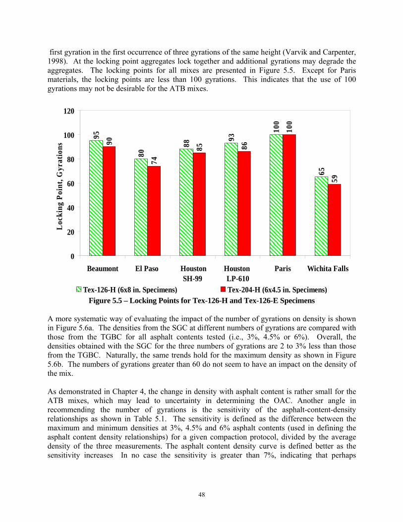
48
first gyration in the first occurrence of three gyrations of the same height (Varvik and Carpenter, 1998). At the locking point aggregates lock together and additional gyrations may degrade the aggregates. The locking points for all mixes are presented in Figure 5.5. Except for Paris materials, the locking points are less than 100 gyrations. This indicates that the use of 100 gyrations may not be desirable for the ATB mixes.
Figure 5.5 – Locking Points for Tex-126-H and Tex-126-E Specimens
A more systematic way of evaluating the impact of the number of gyrations on density is shown in Figure 5.6a. The densities from the SGC at different numbers of gyrations are compared with those from the TGBC for all asphalt contents tested (i.e., 3%, 4.5% or 6%). Overall, the densities obtained with the SGC for the three numbers of gyrations are 2 to 3% less than those from the TGBC. Naturally, the same trends hold for the maximum density as shown in Figure 5.6b. The numbers of gyrations greater than 60 do not seem to have an impact on the density of the mix. As demonstrated in Chapter 4, the change in density with asphalt content is rather small for the ATB mixes, which may lead to uncertainty in determining the OAC. Another angle in recommending the number of gyrations is the sensitivity of the asphalt-content-density relationships as shown in Table 5.1. The sensitivity is defined as the difference between the maximum and minimum densities at 3%, 4.5% and 6% asphalt contents (used in defining the asphalt content density relationships) for a given compaction protocol, divided by the average density of the three measurements. The asphalt content density curve is defined better as the sensitivity increases In no case the sensitivity is greater than 7%, indicating that perhaps
95
80
88
93
100
65
90
74
85 86
100
59
0
20
40
60
80
100
120
Beaumont El Paso Houston SH-99
Houston LP-610
Paris Wichita Falls
Loc
king
Poi
nt, G
yrat
ions
Tex-126-H (6x8 in. Specimens) Tex-204-H (6x4.5 in. Specimens)
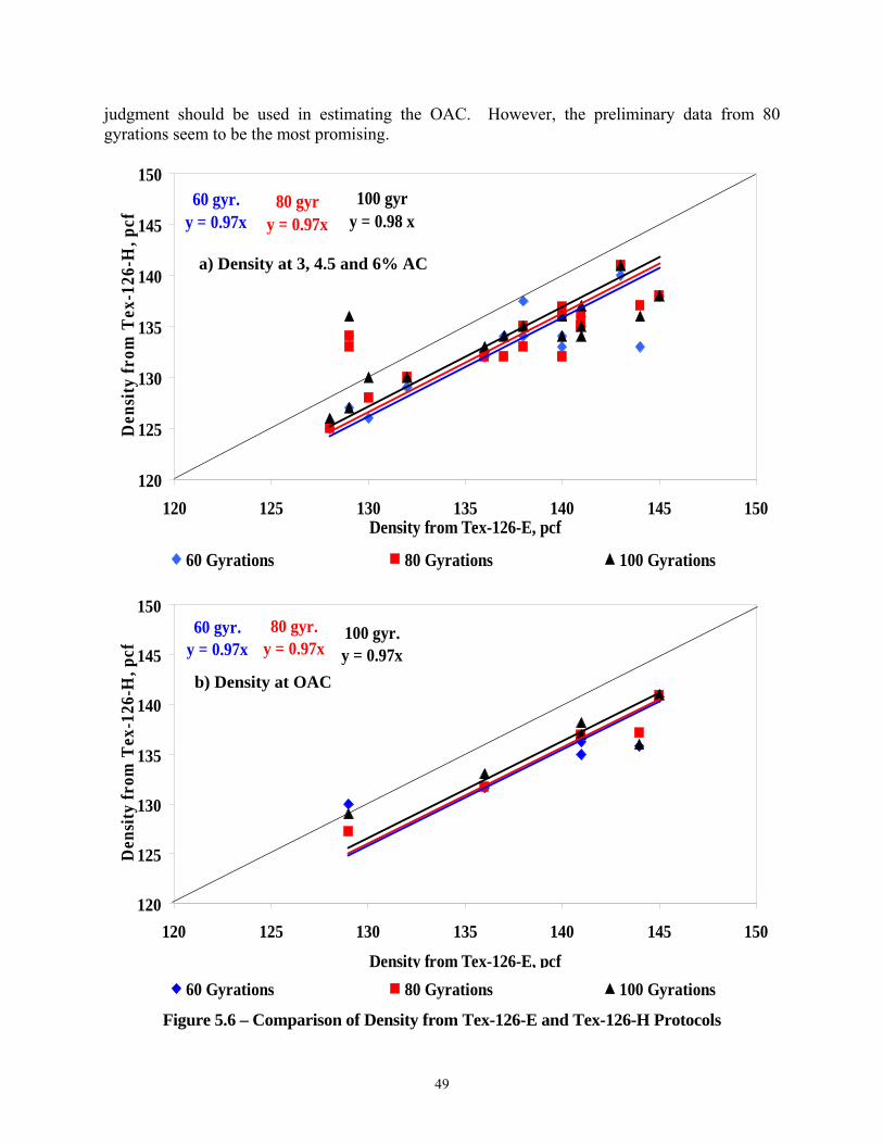
49
judgment should be used in estimating the OAC. However, the preliminary data from 80 gyrations seem to be the most promising.
Figure 5.6 – Comparison of Density from Tex-126-E and Tex-126-H Protocols
60 gyr.y = 0.97x
80 gyry = 0.97x
100 gyry = 0.98 x
120
125
130
135
140
145
150
120 125 130 135 140 145 150Density from Tex-126-E, pcf
Den
sity
fro
m T
ex-1
26-H
, pcf
60 Gyrations 80 Gyrations 100 Gyrations
a)a) Density at 3, 4.5 and 6% AC
80 gyr.y = 0.97x
60 gyr.y = 0.97x
100 gyr.y = 0.97x
120
125
130
135
140
145
150
120 125 130 135 140 145 150
Density from Tex-126-E, pcf
Den
sity
fro
m T
ex-1
26-H
, pcf
60 Gyrations 80 Gyrations 100 Gyrations
b)b) Density at OAC

50
Table 5.1 – Sensitivity of Density to Asphalt Content for Tex-126-H Protocol
Compaction Method
Sensitivity, (Max. Density – Min Density)/Avg. Density
Beaumont El Paso Houston SH-99
Houston LP-610
Paris Wichita
Falls SGC 60 Gyrations 1% 2% 3% 2% 6% 5%
SGC 80 Gyrations 3% 4% 3% 4% 5% 5%
SGC 100 Gyrations 1% 2% 1% 2% 7% 5%
TGBC 3% 5% 4% 1% 1% 6%
Tex-204-H Protocol The impact of the number of gyrations on OAC, density, indirect tensile strength and modulus are summarized in Figures 5.7 to 5.10 for Tex-204-H protocol. As reflected in Figure 5.5, the locking points for this protocol are slightly lower than those for Tex-126-H, perhaps because of the smaller specimen heights 4.5 in. as opposed to 8 in. for Tex-126-H). The trends for the OAC’s (Figure 5.7) are similar to those presented for Tex-126-H in Figure 5.1 except for the Beaumont material. The patterns for the densities (Figure 5.8) at the OAC’s are also similar to those from Tex-126-H. The number of gyrations does not seem to significantly impact the IDT strengths (Figure 5.9) and moduli (Figure 5.10), and the IDT strengths from the SGC and TGBC specimens are closer to one another than the corresponding UCS values from Tex-126-H and Tex-126-E.
Figure 5.7 – Impact of Number of Gyrations on OAC for Tex-204-H Protocol
6.0
4.8
6.0
3.9
6.0
6.0
6.0
5.1
6.0
4.0
6.0
6.0
6.0
3.9
3.8
3.8
6.0
6.0
6.0
5.6
4.7
4.5
4.3
6.0
0
2
4
6
8
Beaumont El Paso Houston SH-99
Houston LP-610
Paris WichitaFalls
Opt
imum
Asp
halt
Con
tent
, %
60 Gyrations 80 Gyrations 100 Gyrations Tex-126-E

51
Figure 5.8 – Impact of Number of Gyrations on Density for Tex-204-H Protocol
Figure 5.9 – Impact of Number of Gyrations on IDT Strength for Tex-204-H Protocol
137 14
1
137
139
127 13
2137 14
1
135 13
9
131
137 13
9
138
139
130 13
4
141 14
5
144
141
129
136
130
100
110
120
130
140
150
160
Beaumont El Paso Houston SH-99
Houston LP-610
Paris WichitaFalls
Den
sity
, pcf
60 Gyrations 80 Gyrations 100 Gyrations Tex-160 Gyrations 80 Gyrations 100 Gyrations Tex-126-E
137 14
1
137
139
127 13
2137 14
1
135 13
9
131
137 13
9
138
139
130 13
4
141 14
5
144
141
129
136
130
100
110
120
130
140
150
160
Beaumont El Paso Houston SH-99
Houston LP-610
Paris WichitaFalls
Den
sity
, pcf
60 Gyrations 80 Gyrations 100 Gyrations Tex-1
137 14
1
137
139
127 13
2137 14
1
135 13
9
131
137 13
9
138
139
130 13
4
141 14
5
144
141
129
136
130
100
110
120
130
140
150
160
Beaumont El Paso Houston SH-99
Houston LP-610
Paris WichitaFalls
Den
sity
, pcf
60 Gyrations 80 Gyrations 100 Gyrations Tex-160 Gyrations 80 Gyrations 100 Gyrations Tex-126-E
103 12
3
20
171
108
186
113 13
3
76
168
119
160
100
130
114
169
101
170
100
73
100
150
115
170
0
50
100
150
200
250
Beaumont El Paso Houston SH-99
Houston LP-610
Paris WichitaFalls
Indi
rect
Ten
sile
Str
engt
h, p
si
60 Gyrations 80 Gyrations 100 Gyrations Tex-12660 Gyrations 80 Gyrations 100 Gyrations Tex-126-E
103 12
3
20
171
108
186
113 13
3
76
168
119
160
100
130
114
169
101
170
100
73
100
150
115
170
0
50
100
150
200
250
Beaumont El Paso Houston SH-99
Houston LP-610
Paris WichitaFalls
Indi
rect
Ten
sile
Str
engt
h, p
si
60 Gyrations 80 Gyrations 100 Gyrations Tex-126
103 12
3
20
171
108
186
113 13
3
76
168
119
160
100
130
114
169
101
170
100
73
100
150
115
170
0
50
100
150
200
250
Beaumont El Paso Houston SH-99
Houston LP-610
Paris WichitaFalls
Indi
rect
Ten
sile
Str
engt
h, p
si
60 Gyrations 80 Gyrations 100 Gyrations Tex-12660 Gyrations 80 Gyrations 100 Gyrations Tex-126-E
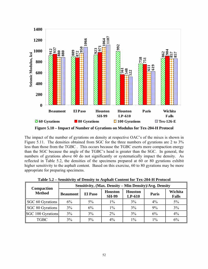
52
Figure 5.10 – Impact of Number of Gyrations on Modulus for Tex-204-H Protocol
The impact of the number of gyrations on density at respective OAC’s of the mixes is shown in Figure 5.11. The densities obtained from SGC for the three numbers of gyrations are 2 to 3% less than those from the TGBC . This occurs because the TGBC exerts more compaction energy than the SGC because the angle of the TGBC’s head is greater than the SGC. In general, the numbers of gyrations above 60 do not significantly or systematically impact the density. As reflected in Table 5.2, the densities of the specimens prepared at 60 or 80 gyrations exhibit higher sensitivity to the asphalt content. Based on this exercise, 60 to 80 gyrations may be more appropriate for preparing specimens.
Table 5.2 – Sensitivity of Density to Asphalt Content for Tex-204-H Protocol
Compaction Method
Sensitivity, (Max. Density – Min Density)/Avg. Density
Beaumont El Paso Houston SH-99
Houston LP-610
Paris Wichita
Falls SGC 60 Gyrations 6% 5% 1% 3% 4% 5%
SGC 80 Gyrations 3% 6% 1% 3% 9% 3%
SGC 100 Gyrations 3% 3% 2% 3% 6% 4%
TGBC 3% 5% 4% 1% 1% 6%
912
889
923 99
2
758 86
2937
872 97
1
561
751
904
880 95
0
1064
548 61
1
857
880
1066 11
07
522 61
9
857
0
200
400
600
800
1000
1200
1400
Beaumont El Paso Houston SH-99
Houston LP-610
Paris WichitaFalls
Sei
smic
Mod
ulu
s, k
si .
60 Gyrations 80 Gyrations 100 Gyrations Tex-126-E
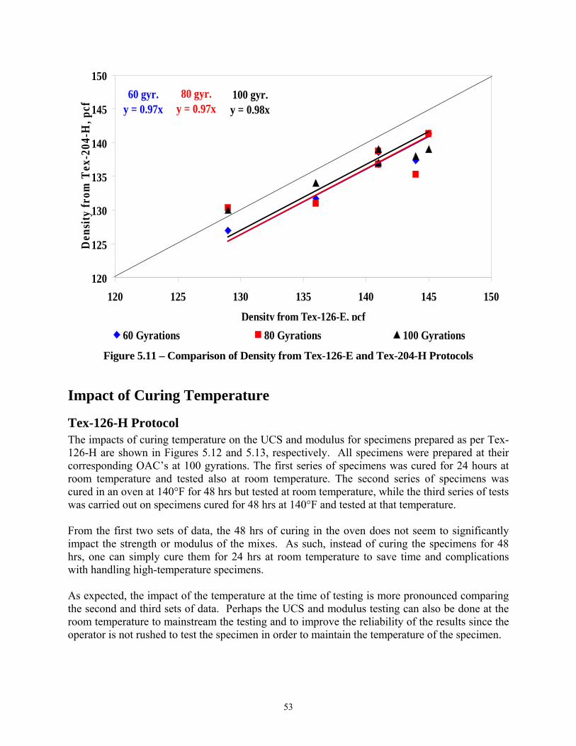
53
Figure 5.11 – Comparison of Density from Tex-126-E and Tex-204-H Protocols
Impact of Curing Temperature
Tex-126-H Protocol The impacts of curing temperature on the UCS and modulus for specimens prepared as per Tex-126-H are shown in Figures 5.12 and 5.13, respectively. All specimens were prepared at their corresponding OAC’s at 100 gyrations. The first series of specimens was cured for 24 hours at room temperature and tested also at room temperature. The second series of specimens was cured in an oven at 140°F for 48 hrs but tested at room temperature, while the third series of tests was carried out on specimens cured for 48 hrs at 140°F and tested at that temperature. From the first two sets of data, the 48 hrs of curing in the oven does not seem to significantly impact the strength or modulus of the mixes. As such, instead of curing the specimens for 48 hrs, one can simply cure them for 24 hrs at room temperature to save time and complications with handling high-temperature specimens. As expected, the impact of the temperature at the time of testing is more pronounced comparing the second and third sets of data. Perhaps the UCS and modulus testing can also be done at the room temperature to mainstream the testing and to improve the reliability of the results since the operator is not rushed to test the specimen in order to maintain the temperature of the specimen.
60 gyr.y = 0.97x
80 gyr.y = 0.97x
100 gyr.y = 0.98x
120
125
130
135
140
145
150
120 125 130 135 140 145 150
Density from Tex-126-E, pcf
Den
sity
fro
m T
ex-2
04-H
, pcf
60 Gyrations 80 Gyrations 100 Gyrations
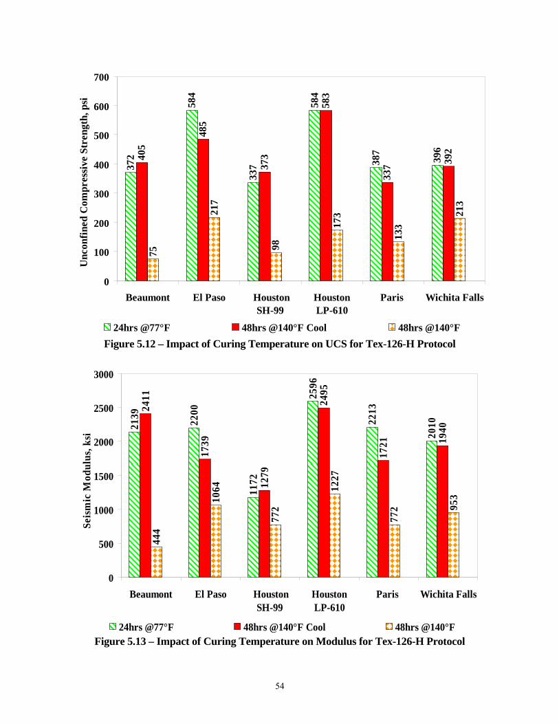
54
Figure 5.12 – Impact of Curing Temperature on UCS for Tex-126-H Protocol
Figure 5.13 – Impact of Curing Temperature on Modulus for Tex-126-H Protocol
372
584
337
584
387
396
405
485
373
583
337 39
2
75
217
98
173
133
213
0
100
200
300
400
500
600
700
Beaumont El Paso Houston SH-99
Houston LP-610
Paris Wichita Falls
Unc
onfi
ned
Com
pres
sive
Str
engt
h, p
si
24hrs @77°F 48hrs @140°F Cool 48hrs @140°F
2139
2200
1172
2596
2213
2010
2411
1739
1279
2495
1721 19
40
444
1064
772
1227
772 95
3
0
500
1000
1500
2000
2500
3000
Beaumont El Paso Houston SH-99
Houston LP-610
Paris Wichita Falls
Seis
mic
Mod
ulus
, ksi
24hrs @77°F 48hrs @140°F Cool 48hrs @140°F
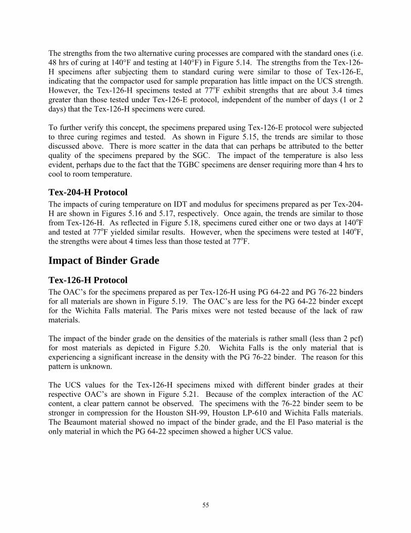
55
The strengths from the two alternative curing processes are compared with the standard ones (i.e. 48 hrs of curing at 140°F and testing at 140°F) in Figure 5.14. The strengths from the Tex-126-H specimens after subjecting them to standard curing were similar to those of Tex-126-E, indicating that the compactor used for sample preparation has little impact on the UCS strength. However, the Tex-126-H specimens tested at 77oF exhibit strengths that are about 3.4 times greater than those tested under Tex-126-E protocol, independent of the number of days (1 or 2 days) that the Tex-126-H specimens were cured. To further verify this concept, the specimens prepared using Tex-126-E protocol were subjected to three curing regimes and tested. As shown in Figure 5.15, the trends are similar to those discussed above. There is more scatter in the data that can perhaps be attributed to the better quality of the specimens prepared by the SGC. The impact of the temperature is also less evident, perhaps due to the fact that the TGBC specimens are denser requiring more than 4 hrs to cool to room temperature.
Tex-204-H Protocol The impacts of curing temperature on IDT and modulus for specimens prepared as per Tex-204-H are shown in Figures 5.16 and 5.17, respectively. Once again, the trends are similar to those from Tex-126-H. As reflected in Figure 5.18, specimens cured either one or two days at 140oF and tested at 77oF yielded similar results. However, when the specimens were tested at 140oF, the strengths were about 4 times less than those tested at 77oF.
Impact of Binder Grade
Tex-126-H Protocol The OAC’s for the specimens prepared as per Tex-126-H using PG 64-22 and PG 76-22 binders for all materials are shown in Figure 5.19. The OAC’s are less for the PG 64-22 binder except for the Wichita Falls material. The Paris mixes were not tested because of the lack of raw materials. The impact of the binder grade on the densities of the materials is rather small (less than 2 pcf) for most materials as depicted in Figure 5.20. Wichita Falls is the only material that is experiencing a significant increase in the density with the PG 76-22 binder. The reason for this pattern is unknown. The UCS values for the Tex-126-H specimens mixed with different binder grades at their respective OAC’s are shown in Figure 5.21. Because of the complex interaction of the AC content, a clear pattern cannot be observed. The specimens with the 76-22 binder seem to be stronger in compression for the Houston SH-99, Houston LP-610 and Wichita Falls materials. The Beaumont material showed no impact of the binder grade, and the El Paso material is the only material in which the PG 64-22 specimen showed a higher UCS value.
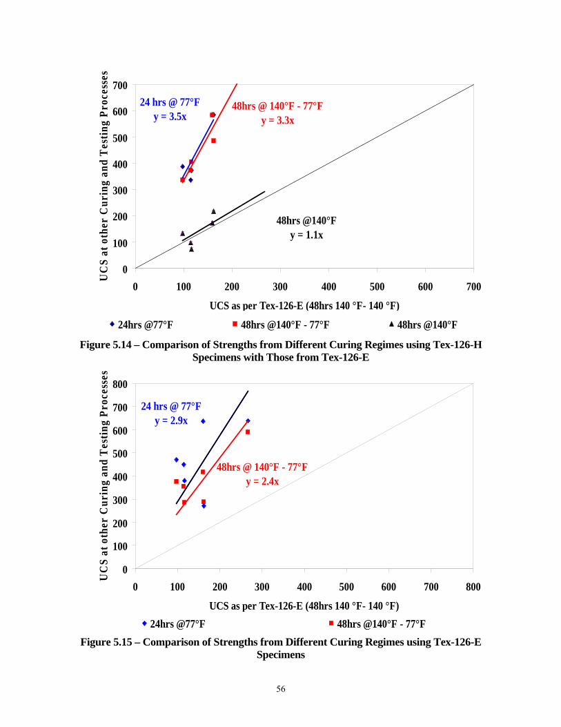
56
Figure 5.14 – Comparison of Strengths from Different Curing Regimes using Tex-126-H
Specimens with Those from Tex-126-E
Figure 5.15 – Comparison of Strengths from Different Curing Regimes using Tex-126-E
Specimens
24 hrs @ 77°Fy = 3.5x
48hrs @ 140°F - 77°Fy = 3.3x
48hrs @140°Fy = 1.1x
0
100
200
300
400
500
600
700
0 100 200 300 400 500 600 700
UCS as per Tex-126-E (48hrs 140 °F- 140 °F)
UC
S at
oth
er C
urin
g an
d T
esti
ng P
roce
sses
24hrs @77°F 48hrs @140°F - 77°F 48hrs @140°F
24 hrs @ 77°Fy = 2.9x
48hrs @ 140°F - 77°Fy = 2.4x
0
100
200
300
400
500
600
700
800
0 100 200 300 400 500 600 700 800
UCS as per Tex-126-E (48hrs 140 °F- 140 °F)
UC
S at
oth
er C
urin
g an
d T
esti
ng P
roce
sses
24hrs @77°F 48hrs @140°F - 77°F
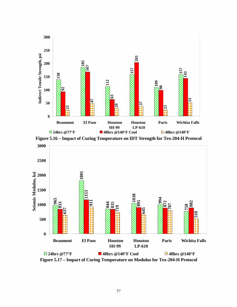
57
Figure 5.16 – Impact of Curing Temperature on IDT Strength for Tex-204-H Protocol
Figure 5.17 – Impact of Curing Temperature on Modulus for Tex-204-H Protocol
138
185
112
157
109
157
92
167
63
203
98
143
22
47
29 37
23
51
0
50
100
150
200
250
300
Beaumont El Paso Houston SH-99
Houston LP-610
Paris Wichita Falls
Indi
rect
Ten
sile
Str
engt
h, p
si
24hrs @77°F 48hrs @140°F Cool 48hrs @140°F
300
138
185
112
157
109
157
92
167
63
203
98
143
22
47
29 37
23
51
0
50
100
150
200
250
300
Beaumont El Paso Houston SH-99
Houston LP-610
Paris Wichita Falls
Indi
rect
Ten
sile
Str
engt
h, p
si
24hrs @77°F 48hrs @140°F Cool 48hrs @140°F
138
185
112
157
109
157
92
167
63
203
98
143
22
47
29 37
23
51
0
50
100
150
200
250
300
Beaumont El Paso Houston SH-99
Houston LP-610
Paris Wichita Falls
Indi
rect
Ten
sile
Str
engt
h, p
si
24hrs @77°F 48hrs @140°F Cool 48hrs @140°F
300
965
1801
844 10
38
994
75883
3
1153
835
895
872
882
637
911
719
645 78
7
510
0
500
1000
1500
2000
2500
3000
Beaumont El Paso Houston SH-99
Houston LP-610
Paris Wichita Falls
Seis
mic
Mod
ulus
, ksi
24hrs @77°F 48hrs @140°F Cool 48hrs @140°F
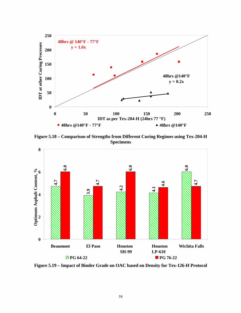
58
Figure 5.18 – Comparison of Strengths from Different Curing Regimes using Tex-204-H
Specimens
Figure 5.19 – Impact of Binder Grade on OAC based on Density for Tex-126-H Protocol
48hrs @ 140°F - 77°Fy = 1.0x
48hrs @140°Fy = 0.2x
0
50
100
150
200
250
0 50 100 150 200 250IDT as per Tex-204-H (24hrs 77 °F)
IDT
at
othe
r C
urin
g P
roce
sses
48hrs @140°F - 77°F 48hrs @140°F
4.7
3.9 4.
2
4.1
6.0
6.0
4.7
6.0
4.6 4.7
0
2
4
6
8
Beaumont El Paso Houston SH-99
Houston LP-610
Wichita Falls
Opt
imum
Asp
halt
Con
tent
, %
PG 64-22 PG 76-22
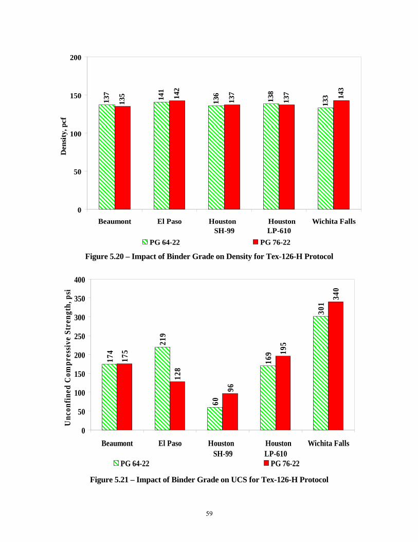
59
Figure 5.20 – Impact of Binder Grade on Density for Tex-126-H Protocol
Figure 5.21 – Impact of Binder Grade on UCS for Tex-126-H Protocol
137
141
136
138
133
135 14
2
137
137 14
3
0
50
100
150
200
Beaumont El Paso Houston SH-99
Houston LP-610
Wichita Falls
Den
sity
, pcf
PG 64-22 PG 76-22
174
219
60
169
301
175
128
96
195
340
0
50
100
150
200
250
300
350
400
Beaumont El Paso Houston SH-99
Houston LP-610
Wichita Falls
Unc
onfi
ned
Com
pres
sive
Str
engt
h, p
si
PG 64-22 PG 76-22

60
Tex- 204-H Protocol The OAC’s based on density obtained from the two binders from the Tex-204-H protocol are compared in Figure 5.22. In this case, the OAC’s from the two binders are closer to one another. As shown in Figure 5.23, the densities were not impacted significantly by the binder grade. They are generally within 3 pcf of one another. The impact of the binder grade on the IDT strengths is shown in Figure 5.24. Unlike the UCS trends in Figure 5.21, the PG 76-22 specimens seem to be stronger under tension as compared to the PG 64-22 specimens for almost all materials. The trends for seismic moduli, as shown in Figure 5.25, are different. The reason for this contradiction is that the modulus is more indicative of the compressive strength than the tensile strength.
Impact of AC Content Each material was tested at its OAC and ±1 of its OAC to observe how the change in binder content will impact the behavior of the mix. The specimens were cured for 24 hrs and tested at 77°F. The variations in the UCS with asphalt content for Tex-126-H specimens are shown in Figure 5.26. Most materials are stronger either at the OAC or 1% less than OAC. A clear pattern is not obvious because as indicated in Chapter 4 the selection of OAC based on the density is rather uncertain. The modulus pattern is not that different as shown in Figure 5.27. The IDT strengths and seismic moduli for the Tex-204-H specimens are shown in Figures 5.28 and 5.29, respectively. In most cases, the change in AC content does not seem to impact the IDT strength and modulus much.
Impact of Gradation Up to this point, all the specimens were molded using the in place gradation of the materials as delivered to UTEP. As indicated in Chapter 4, those gradations met the Item 344 gradations. A second gradation that was compatible with Item 292 was developed for each material by increasing the fine contents in order to quantify the importance of the gradation in a mix. As reflected in Table 5.3, the modified gradations (values in parenthesis) were obtained by modifying only the materials finer than No. 40 Sieve so that 15% of the materials passed the number 200 sieve (while the original gradation contained less than 5%). This experiment was carried out on four materials.
Tex-126-H Protocol Figure 5.30 compares the OACs for the Tex-126-H protocol from the two different gradations used. The quantities of the asphalt needed to achieve the maximum density for the Item 292 gradations are higher or close to those from the Item 344 gradations. The changes in maximum densities are not significant as the fines content increases, but the high fines content specimens’ densities were found equal or slightly higher than the densities of the original gradations (see Figure 5.31).

61
Figure 5.22 – Impact of Binder Grade on OAC for Tex-204-H Protocol
Figure 5.23 – Impact of Binder Grade on Density for Tex-204-H Protocol
6.0
3.9
3.8
3.8
6.0
6.0
4.1
4.8
4.2
5.3
0
2
4
6
8
Beaumont El Paso Houston SH-99
Houston LP-610
Wichita Falls
Opt
imum
Asp
halt
Con
tent
, %
PG 64-22 PG 76-22
137
139
138
139
134
136
140 14
6
136
134
0
50
100
150
200
Beaumont El Paso Houston SH-99
Houston LP-610
Wichita Falls
Den
sity
, pcf
PG 64-22 PG 76-22
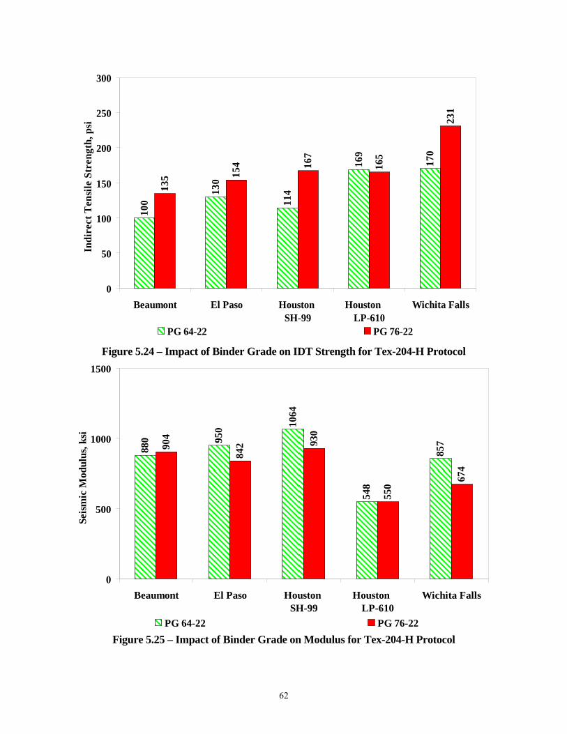
62
Figure 5.24 – Impact of Binder Grade on IDT Strength for Tex-204-H Protocol
Figure 5.25 – Impact of Binder Grade on Modulus for Tex-204-H Protocol
100
130
114
169
170
135 15
4 167
165
231
0
50
100
150
200
250
300
Beaumont El Paso Houston SH-99
Houston LP-610
Wichita Falls
Indi
rect
Ten
sile
Str
engt
h, p
si
PG 64-22 PG 76-22
880 95
0 1064
548
85790
4
842 93
0
550
674
0
500
1000
1500
Beaumont El Paso Houston SH-99
Houston LP-610
Wichita Falls
Seis
mic
Mod
ulus
, ksi
PG 64-22 PG 76-22

63
Figure 5.26 – Impact of Asphalt Content Variation on UCS for Tex-126-H Protocol
Figure 5.27 – Impact of Asphalt Content Variation on Modulus for Tex-126-H Protocol
410
591
227
418
342
590
372
584
337
584
387
396
394
380
231
325
331
411
0
100
200
300
400
500
600
700
Beaumont El Paso Houston SH-99
Houston LP-610
Paris WichitaFalls
Unc
onfi
ned
Com
pres
sive
Str
engt
h, p
si
(-) 1% OAC % (+) 1 %
1715
852
1946
2360
1808
2139
2200
1172
2596
2213
201021
51
1229
1994
2461
2001 22
30
2654
0
500
1000
1500
2000
2500
3000
Beaumont El Paso Houston SH-99
Houston LP-610
Paris WichitaFalls
Seis
mic
Mod
ulus
, ksi
(-) 1% OAC % (+) 1 %
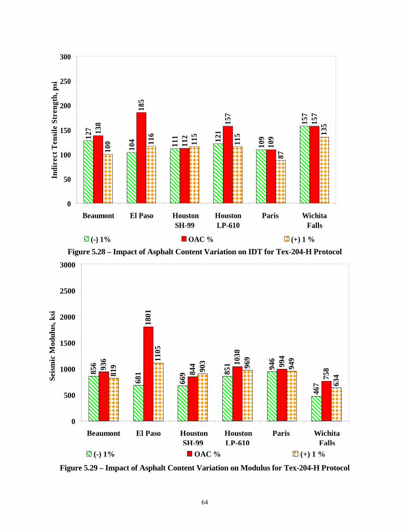
64
Figure 5.28 – Impact of Asphalt Content Variation on IDT for Tex-204-H Protocol
Figure 5.29 – Impact of Asphalt Content Variation on Modulus for Tex-204-H Protocol
127
104 111 12
1
109
157
138
185
112
157
109
157
100 11
6
115
115
87
135
0
50
100
150
200
250
300
Beaumont El Paso Houston SH-99
Houston LP-610
Paris WichitaFalls
Indi
rect
Ten
sile
Str
engt
h, p
si
(-) 1% OAC % (+) 1 %
856
681
669 85
1 946
467
936
1801
844 10
38
994
758
819
1105
903 969
949
634
0
500
1000
1500
2000
2500
3000
Beaumont El Paso Houston SH-99
Houston LP-610
Paris WichitaFalls
Seis
mic
Mod
ulus
, ksi
(-) 1% OAC % (+) 1 %
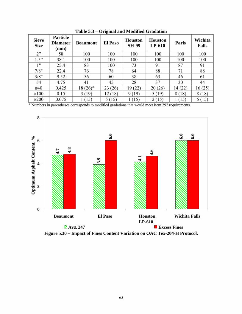
65
Table 5.3 – Original and Modified Gradation
Sieve Size
Particle Diameter
(mm) Beaumont El Paso
Houston SH-99
Houston LP-610
Paris Wichita
Falls
2” 58 100 100 100 100 100 100 1.5” 38.1 100 100 100 100 100 100 1" 25.4 83 100 73 91 87 91
7/8" 22.4 76 78 64 88 71 88 3/8" 9.52 56 60 38 63 46 61 #4 4.75 41 45 28 37 30 44 #40 0.425 18 (26)* 23 (26) 19 (22) 20 (26) 14 (22) 16 (25) #100 0.15 3 (19) 12 (18) 9 (19) 5 (19) 8 (18) 8 (18) #200 0.075 1 (15) 5 (15) 1 (15) 2 (15) 1 (15) 5 (15)
* Numbers in parentheses corresponds to modified gradations that would meet Item 292 requirements.
Figure 5.30 – Impact of Fines Content Variation on OAC Tex-204-H Protocol.
4.7
3.9 4.
1
6.0
4.8
6.0
4.6
6.0
0
2
4
6
8
Beaumont El Paso Houston LP-610
Wichita Falls
Opt
imum
Asp
halt
Con
tent
, %
Avg. 247 Excess Fines
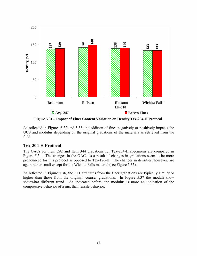
66
Figure 5.31 – Impact of Fines Content Variation on Density Tex-204-H Protocol.
As reflected in Figures 5.32 and 5.33, the addition of fines negatively or positively impacts the UCS and modulus depending on the original gradations of the materials as retrieved from the field.
Tex-204-H Protocol The OACs for Item 292 and Item 344 gradations for Tex-204-H specimens are compared in Figure 5.34. The changes in the OACs as a result of changes in gradations seem to be more pronounced for this protocol as opposed to Tex-126-H. The changes in densities, however, are again rather small except for the Wichita Falls material (see Figure 5.35).
As reflected in Figure 5.36, the IDT strengths from the finer gradations are typically similar or higher than those from the original, coarser gradations. In Figure 5.37 the moduli show somewhat different trend. As indicated before, the modulus is more an indication of the compressive behavior of a mix than tensile behavior.
137
141
138
13313
9 148
140
133
0
50
100
150
200
Beaumont El Paso Houston LP-610
Wichita Falls
Den
sity
, pcf
Avg. 247 Excess Fines

67
Figure 5.32 – Impact of Fines Content Variation on UCS Tex-126-H Protocol.
Figure 5.33 – Impact of Fines Content Variation on Modulus for Tex-126-H Protocol.
174
219
169
301
233
91
195 20
9
0
50
100
150
200
250
300
350
Beaumont El Paso Houston LP-610
Wichita Falls
Unc
onfi
ned
Com
pres
sive
Str
engt
h, p
si
Avg. 247 Excess Fines
874
615
1032
1524
879
510
977
883
0
300
600
900
1200
1500
1800
Beaumont El Paso Houston LP-610
Wichita Falls
Seis
mic
Mod
ulus
, ksi
Avg. 247 Excess Fines
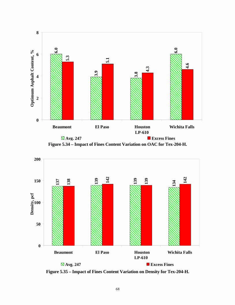
68
Figure 5.34 – Impact of Fines Content Variation on OAC for Tex-204-H.
Figure 5.35 – Impact of Fines Content Variation on Density for Tex-204-H.
6.0
3.9
3.8
6.0
5.3
5.1
4.3 4.
6
0
2
4
6
8
Beaumont El Paso Houston LP-610
Wichita Falls
Opt
imum
Asp
halt
Con
tent
, %
Avg. 247 Excess Fines
137
139
139
134
138 142
139
142
0
50
100
150
200
Beaumont El Paso Houston LP-610
Wichita Falls
Den
sity
, pcf
Avg. 247 Excess Fines

69
Figure 5.36 – Impact of Fines Content Variation on IDT for Tex-204-H.
Figure 5.37 – Impact of Fines Content Variation on Modulus for Tex-204-H.
100
130
169
170
206
146
165
205
0
50
100
150
200
250
Beaumont El Paso Houston LP-610
Wichita Falls
Indi
rect
Ten
sile
Str
engt
h, p
si
Avg. 247 Excess Fines
880 95
0
548
85794
4
1179
900
670
0
300
600
900
1200
1500
1800
Beaumont El Paso Houston LP-610
Wichita Falls
Seis
mic
Mod
ulus
, ksi
Avg. 247 Excess Fines
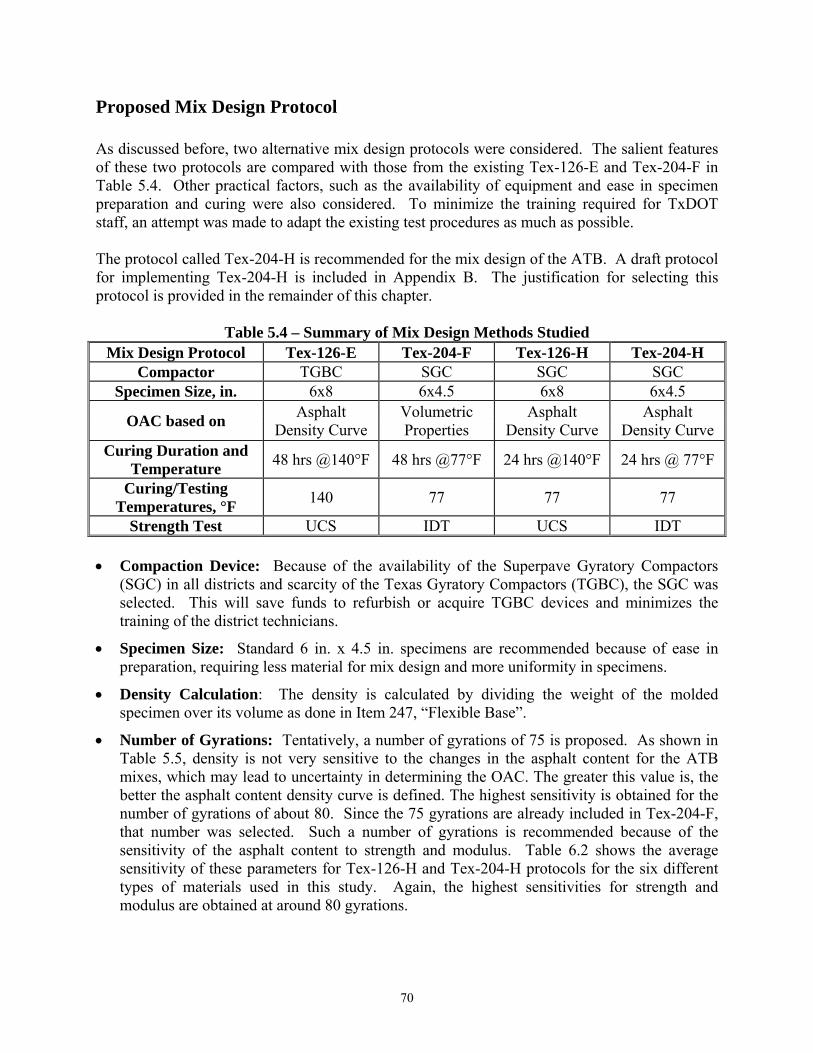
70
Proposed Mix Design Protocol As discussed before, two alternative mix design protocols were considered. The salient features of these two protocols are compared with those from the existing Tex-126-E and Tex-204-F in Table 5.4. Other practical factors, such as the availability of equipment and ease in specimen preparation and curing were also considered. To minimize the training required for TxDOT staff, an attempt was made to adapt the existing test procedures as much as possible. The protocol called Tex-204-H is recommended for the mix design of the ATB. A draft protocol for implementing Tex-204-H is included in Appendix B. The justification for selecting this protocol is provided in the remainder of this chapter.
Table 5.4 – Summary of Mix Design Methods Studied
Mix Design Protocol Tex-126-E Tex-204-F Tex-126-H Tex-204-H Compactor TGBC SGC SGC SGC
Specimen Size, in. 6x8 6x4.5 6x8 6x4.5
OAC based on Asphalt
Density Curve Volumetric Properties
Asphalt Density Curve
Asphalt Density Curve
Curing Duration and Temperature
48 hrs @140°F 48 hrs @77°F 24 hrs @140°F 24 hrs @ 77°F
Curing/Testing Temperatures, °F
140 77 77 77
Strength Test UCS IDT UCS IDT Compaction Device: Because of the availability of the Superpave Gyratory Compactors
(SGC) in all districts and scarcity of the Texas Gyratory Compactors (TGBC), the SGC was selected. This will save funds to refurbish or acquire TGBC devices and minimizes the training of the district technicians.
Specimen Size: Standard 6 in. x 4.5 in. specimens are recommended because of ease in preparation, requiring less material for mix design and more uniformity in specimens.
Density Calculation: The density is calculated by dividing the weight of the molded specimen over its volume as done in Item 247, “Flexible Base”.
Number of Gyrations: Tentatively, a number of gyrations of 75 is proposed. As shown in Table 5.5, density is not very sensitive to the changes in the asphalt content for the ATB mixes, which may lead to uncertainty in determining the OAC. The greater this value is, the better the asphalt content density curve is defined. The highest sensitivity is obtained for the number of gyrations of about 80. Since the 75 gyrations are already included in Tex-204-F, that number was selected. Such a number of gyrations is recommended because of the sensitivity of the asphalt content to strength and modulus. Table 6.2 shows the average sensitivity of these parameters for Tex-126-H and Tex-204-H protocols for the six different types of materials used in this study. Again, the highest sensitivities for strength and modulus are obtained at around 80 gyrations.
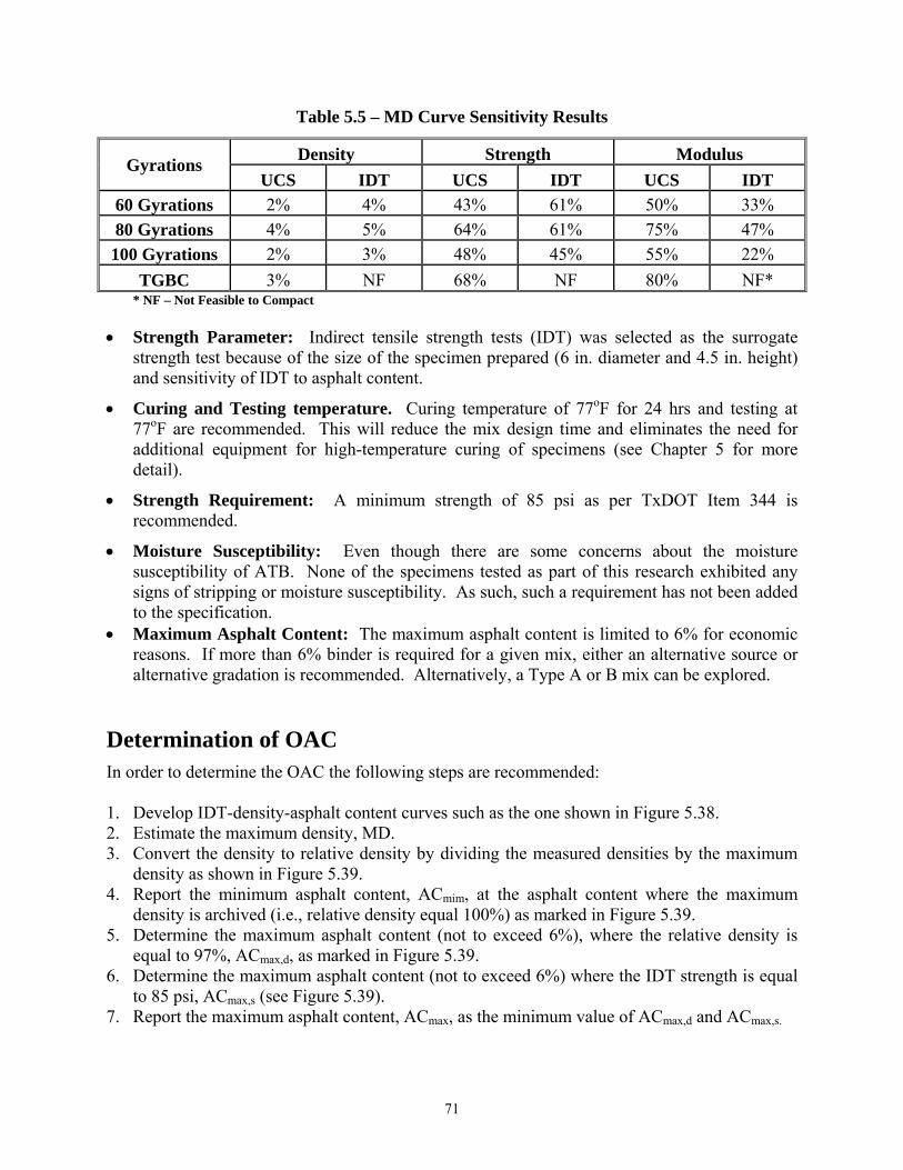
71
Table 5.5 – MD Curve Sensitivity Results
* NF – Not Feasible to Compact
Strength Parameter: Indirect tensile strength tests (IDT) was selected as the surrogate strength test because of the size of the specimen prepared (6 in. diameter and 4.5 in. height) and sensitivity of IDT to asphalt content.
Curing and Testing temperature. Curing temperature of 77oF for 24 hrs and testing at 77oF are recommended. This will reduce the mix design time and eliminates the need for additional equipment for high-temperature curing of specimens (see Chapter 5 for more detail).
Strength Requirement: A minimum strength of 85 psi as per TxDOT Item 344 is recommended.
Moisture Susceptibility: Even though there are some concerns about the moisture susceptibility of ATB. None of the specimens tested as part of this research exhibited any signs of stripping or moisture susceptibility. As such, such a requirement has not been added to the specification.
Maximum Asphalt Content: The maximum asphalt content is limited to 6% for economic reasons. If more than 6% binder is required for a given mix, either an alternative source or alternative gradation is recommended. Alternatively, a Type A or B mix can be explored.
Determination of OAC In order to determine the OAC the following steps are recommended: 1. Develop IDT-density-asphalt content curves such as the one shown in Figure 5.38. 2. Estimate the maximum density, MD. 3. Convert the density to relative density by dividing the measured densities by the maximum
density as shown in Figure 5.39. 4. Report the minimum asphalt content, ACmim, at the asphalt content where the maximum
density is archived (i.e., relative density equal 100%) as marked in Figure 5.39. 5. Determine the maximum asphalt content (not to exceed 6%), where the relative density is
equal to 97%, ACmax,d, as marked in Figure 5.39. 6. Determine the maximum asphalt content (not to exceed 6%) where the IDT strength is equal
to 85 psi, ACmax,s (see Figure 5.39). 7. Report the maximum asphalt content, ACmax, as the minimum value of ACmax,d and ACmax,s.
Gyrations Density Strength Modulus
UCS IDT UCS IDT UCS IDT
60 Gyrations 2% 4% 43% 61% 50% 33%
80 Gyrations 4% 5% 64% 61% 75% 47%
100 Gyrations 2% 3% 48% 45% 55% 22%
TGBC 3% NF 68% NF 80% NF*
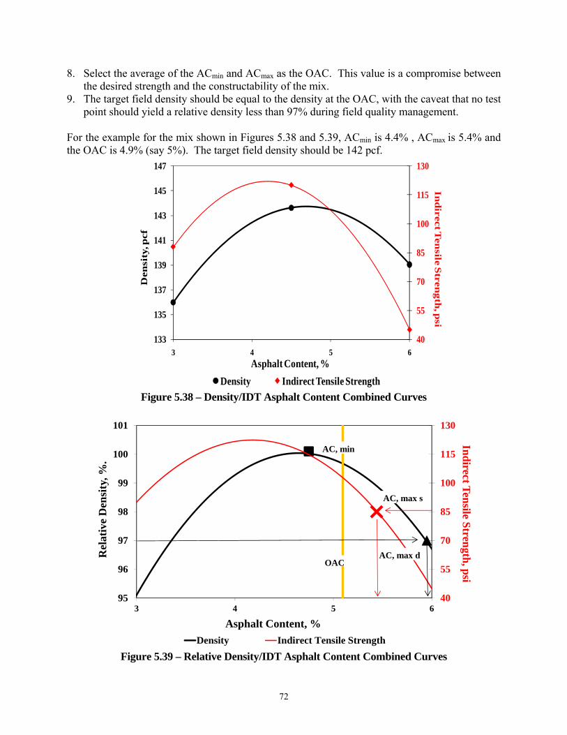
72
8. Select the average of the ACmin and ACmax as the OAC. This value is a compromise between the desired strength and the constructability of the mix.
9. The target field density should be equal to the density at the OAC, with the caveat that no test point should yield a relative density less than 97% during field quality management.
For the example for the mix shown in Figures 5.38 and 5.39, ACmin is 4.4% , ACmax is 5.4% and the OAC is 4.9% (say 5%). The target field density should be 142 pcf.
Figure 5.38 – Density/IDT Asphalt Content Combined Curves
Figure 5.39 – Relative Density/IDT Asphalt Content Combined Curves
40
55
70
85
100
115
130
133
135
137
139
141
143
145
147
3 4 5 6
Ind
irect Ten
sile Stren
gth
, psi
Den
sity
, pcf
Asphalt Content, %
Density Indirect Tensile Strength
40
55
70
85
100
115
130
95
96
97
98
99
100
101
3 4 5 6
Ind
irect Ten
sile Stren
gth, p
si R
elat
ive
Den
sity
, %.
Asphalt Content, %
Density Indirect Tensile Strength
AC, max s
AC, min
OACAC, max d

73
CHAPTER SIX – FIELD PERFORMANCE MONITORING In this chapter the information obtained from field investigation conducted before, during and after construction at five sites is presented. Figure 6.1 shows the locations of the five sites that were monitored. These sites were located in Alpine in El Paso District, Beltway 8 and FM 526 (Federal Rd) in Houston District, and FM 943 and FM 2798 in Beaumont District. The pavement profile of each site is shown in Figure 6.2. The ATB layers varied in thickness between 8 in. and 10 in. All sites were covered with surface treatment, expect for Alpine that the ATB was covered with a concrete slab, and Houston Beltway 8 that the ATB was not covered at all. Materials used to produce the mixture were collected from the plants for laboratory tests. During construction, plant-produced mixtures were also collected and taken to the laboratory for index and strength tests. A Portable Seismic Property Analyzer (PSPA) was used about 24 hrs, 6 months and 12 months after field compaction at selected stations. Falling Weight Deflectometer (FWD) tests were performed approximately 6 and 12 months after construction. Cores were also extracted from most sites at selected stations. The laboratory and field properties were compared with the materials and information gathered at each site. The results and conclusions of this activity are presented in this chapter.
Laboratory Results
Raw Materials
The gradation curves of the combined blend from materials collected at the quarries are shown in Figure 6.3. Since the same quarry materials were used for both projects in Houston and Beaumont, only one mix design was used for each district. To prepare the mix design from each source, the entire stock was sieved first to develop a global gradation curve. That gradation curve was used throughout the study. The acceptable tolerances as per Item 292 Grade 1 are also shown in the figure. All gradation curves met the requirements of Item 292. As shown in Table 6.1, the Alpine materials had a Plasticity Index (PI) of 4 while Beaumont and Houston materials were non-plastic. The sand equivalency and aggregate hardness for each material are also presented in Table 6.1. The Houston and Beaumont materials met the sand
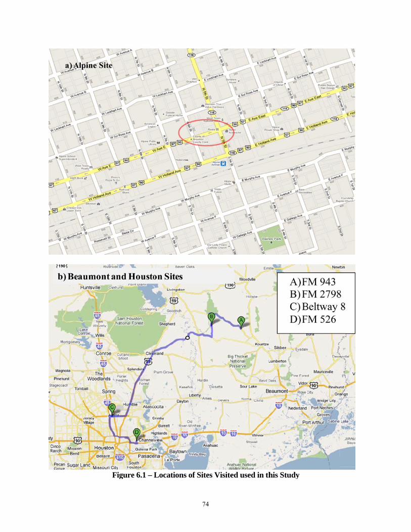
FFigure 6.1 – Locations o
74
f Sites Visiteed used in thhis Study
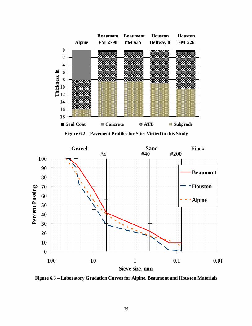
75
Figure 6.2 – Pavement Profiles for Sites Visited in this Study
Figure 6.3 – Laboratory Gradation Curves for Alpine, Beaumont and Houston Materials
0
2
4
6
8
10
12
14
16
18
AlpineBeaumontFM 2798
BeaumontSH 943
HoustonBeltway 8
HoustonFM 526
Th
ick
nes
s, in
Seal Coat Concrete ATB Subgrade
0
10
20
30
40
50
60
70
80
90
100
0.010.1110100Sieve size, mm
Per
cen
t P
assi
ng
Beaumont
Houston
Alpine
#4 #40 #200Gravel Sand Fines
FM 943
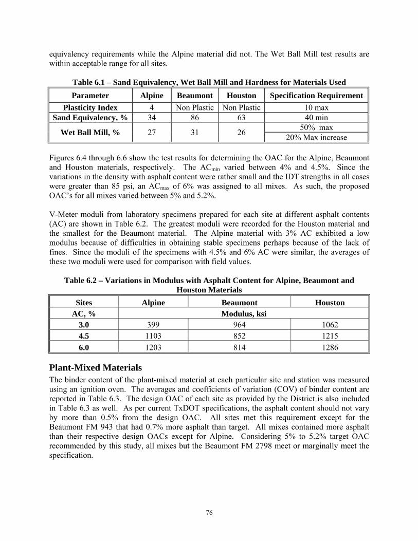
76
equivalency requirements while the Alpine material did not. The Wet Ball Mill test results are within acceptable range for all sites.
Table 6.1 – Sand Equivalency, Wet Ball Mill and Hardness for Materials Used
Parameter Alpine Beaumont Houston Specification Requirement
Plasticity Index 4 Non Plastic Non Plastic 10 max Sand Equivalency, % 34 86 63 40 min
Wet Ball Mill, % 27 31 26 50% max
20% Max increase Figures 6.4 through 6.6 show the test results for determining the OAC for the Alpine, Beaumont and Houston materials, respectively. The ACmin varied between 4% and 4.5%. Since the variations in the density with asphalt content were rather small and the IDT strengths in all cases were greater than 85 psi, an ACmax of 6% was assigned to all mixes. As such, the proposed OAC’s for all mixes varied between 5% and 5.2%. V-Meter moduli from laboratory specimens prepared for each site at different asphalt contents (AC) are shown in Table 6.2. The greatest moduli were recorded for the Houston material and the smallest for the Beaumont material. The Alpine material with 3% AC exhibited a low modulus because of difficulties in obtaining stable specimens perhaps because of the lack of fines. Since the moduli of the specimens with 4.5% and 6% AC were similar, the averages of these two moduli were used for comparison with field values.
Table 6.2 – Variations in Modulus with Asphalt Content for Alpine, Beaumont and Houston Materials
Sites Alpine Beaumont Houston AC, % Modulus, ksi
3.0 399 964 1062 4.5 1103 852 1215
6.0 1203 814 1286
Plant-Mixed Materials The binder content of the plant-mixed material at each particular site and station was measured using an ignition oven. The averages and coefficients of variation (COV) of binder content are reported in Table 6.3. The design OAC of each site as provided by the District is also included in Table 6.3 as well. As per current TxDOT specifications, the asphalt content should not vary by more than 0.5% from the design OAC. All sites met this requirement except for the Beaumont FM 943 that had 0.7% more asphalt than target. All mixes contained more asphalt than their respective design OACs except for Alpine. Considering 5% to 5.2% target OAC recommended by this study, all mixes but the Beaumont FM 2798 meet or marginally meet the specification.
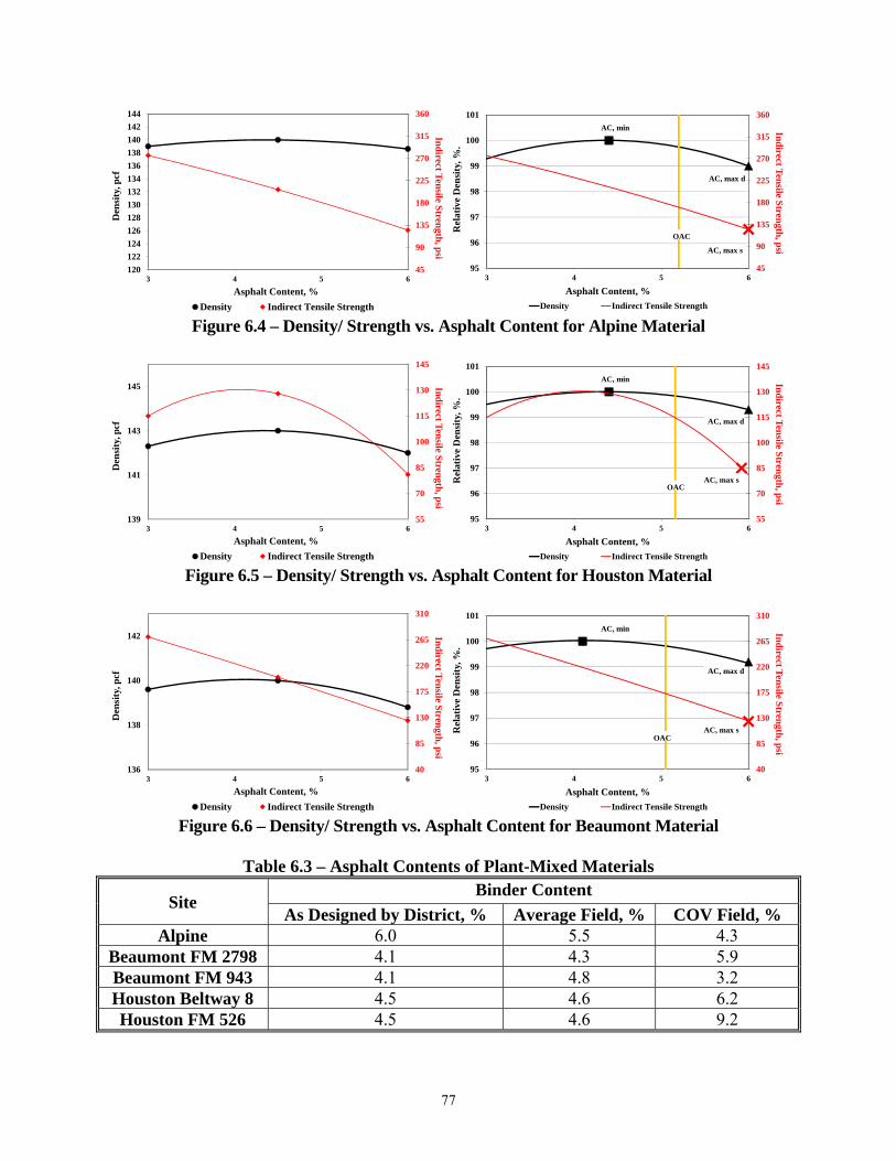
77
Figure 6.4 – Density/ Strength vs. Asphalt Content for Alpine Material
Figure 6.5 – Density/ Strength vs. Asphalt Content for Houston Material
Figure 6.6 – Density/ Strength vs. Asphalt Content for Beaumont Material
Table 6.3 – Asphalt Contents of Plant-Mixed Materials
Site Binder Content
As Designed by District, % Average Field, % COV Field, % Alpine 6.0 5.5 4.3
Beaumont FM 2798 4.1 4.3 5.9 Beaumont FM 943 4.1 4.8 3.2 Houston Beltway 8 4.5 4.6 6.2 Houston FM 526 4.5 4.6 9.2
45
90
135
180
225
270
315
360
95
96
97
98
99
100
101
3 4 5 6
Ind
irect Ten
sile Stren
gth, p
si
Rel
ativ
e D
ensi
ty, %
.
Asphalt Content, %
Density Indirect Tensile Strength
AC, max s
AC, min
OAC
AC, max d
45
90
135
180
225
270
315
360
120
122
124
126
128
130
132
134
136
138
140
142
144
3 4 5 6
Ind
irect Ten
sile Stren
gth, p
si
Den
sity
, pcf
Asphalt Content, %
Density Indirect Tensile Strength
55
70
85
100
115
130
145
95
96
97
98
99
100
101
3 4 5 6
Indirect Tensile Strength
, psi
Rel
ativ
e D
ensi
ty, %
.
Asphalt Content, %
Density Indirect Tensile Strength
AC, max s
AC, min
OAC
AC, max d
55
70
85
100
115
130
145
139
141
143
145
3 4 5 6
Indirect Tensile Strength
, psi
Den
sity
, pcf
Asphalt Content, %
Density Indirect Tensile Strength
40
85
130
175
220
265
310
95
96
97
98
99
100
101
3 4 5 6
Ind
irect Ten
sile Stren
gth, p
si
Rel
ativ
e D
ensi
ty, %
.
Asphalt Content, %
Density Indirect Tensile Strength
AC, max s
AC, min
OAC
AC, max d
40
85
130
175
220
265
310
136
138
140
142
3 4 5 6
Ind
irect Ten
sile Stren
gth, p
si
Den
sity
, pcf
Asphalt Content, %
Density Indirect Tensile Strength
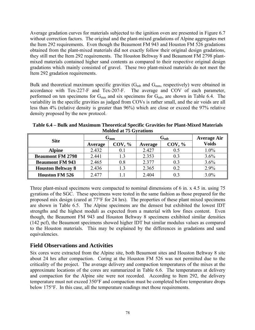
78
Average gradation curves for materials subjected to the ignition oven are presented in Figure 6.7 without correction factors. The original and the plant-mixed gradations of Alpine aggregates met the Item 292 requirements. Even though the Beaumont FM 943 and Houston FM 526 gradations obtained from the plant-mixed materials did not exactly follow their original design gradations, they still met the Item 292 requirements. The Houston Beltway 8 and Beaumont FM 2798 plant-mixed materials contained higher sand contents as compared to their respective original design gradations which mainly consisted of gravel. These two plant-mixed materials do not meet the Item 292 gradation requirements. Bulk and theoretical maximum specific gravities (Gmb and Gmm, respectively) were obtained in accordance with Tex-227-F and Tex-207-F. The average and COV of each parameter, performed on ten specimens for Gmm and six specimens for Gmb, are shown in Table 6.4. The variability in the specific gravities as judged from COVs is rather small, and the air voids are all less than 4% (relative density is greater than 96%) which are close or exceed the 97% relative density proposed by the new protocol.
Table 6.4 – Bulk and Maximum Theoretical Specific Gravities for Plant-Mixed Materials
Molded at 75 Gyrations
Site Gmm Gmb Average Air
Voids Average COV, % Average COV, % Alpine 2.432 0.1 2.427 0.5 1.0%
Beaumont FM 2798 2.441 1.3 2.353 0.3 3.6% Beaumont FM 943 2.465 0.8 2.377 0.3 3.6% Houston Beltway 8 2.436 1.3 2.365 0.2 2.9% Houston FM 526 2.477 1.1 2.404 0.3 3.0%
Three plant-mixed specimens were compacted to nominal dimensions of 6 in. x 4.5 in. using 75 gyrations of the SGC. These specimens were tested in the same fashion as those prepared for the proposed mix design (cured at 77°F for 24 hrs). The properties of these plant mixed specimens are shown in Table 6.5. The Alpine specimens are the densest but exhibited the lowest IDT strengths and the highest moduli as expected from a material with low fines content. Even though, the Beaumont FM 943 and Houston Beltway 8 specimens exhibited similar densities (142 pcf), the Beaumont specimens showed higher IDT but similar modulus values as compared to the Houston materials. This may be explained by the differences in gradations and sand equivalencies.
Field Observations and Activities Six cores were extracted from the Alpine site, both Beaumont sites and Houston Beltway 8 site about 24 hrs after compaction. Coring at the Houston FM 526 was not permitted due to the criticality of the project. The average delivery and compaction temperatures of the mixes at the approximate locations of the cores are summarized in Table 6.6. The temperatures at delivery and compaction for the Alpine site were not recorded. According to Item 292, the delivery temperature must not exceed 350°F and compaction must be completed before temperature drops below 175°F. In this case, all the temperature readings met those requirements.

79
Figure 6.1 – Gradation Curves from Plant-Mixed Materials as Delivered
0
10
20
30
40
50
60
70
80
90
100
0.010.1110100
Per
cen
t P
assi
ng
Sieve size, mm
Original
Plant-Mixed FM 3513
Field Cores FM 3513
Plant-Mixed FM 2798
Field Cores FM 2798
#4 #40 #200Gravel Sand Fines
b) Beaumont Material
Plant-Mixed FM 943
Field Cores FM 943
0
10
20
30
40
50
60
70
80
90
100
0.010.1110100
Per
cen
t P
assi
ng
Sieve size, mm
Original
Plant-Mixed
Field Cores
#4 #40 #200Gravel Sand Fines
a) Alpine Material
0
10
20
30
40
50
60
70
80
90
100
0.010.1110100
Per
cen
t P
assi
ng
Sieve size, mm
Original
Plant-Mixed FM 526
Plant-Mixed Beltway 8
Field Cores Beltway 8
#4 #40 #200Gravel Sand Fines
c) Houston Material
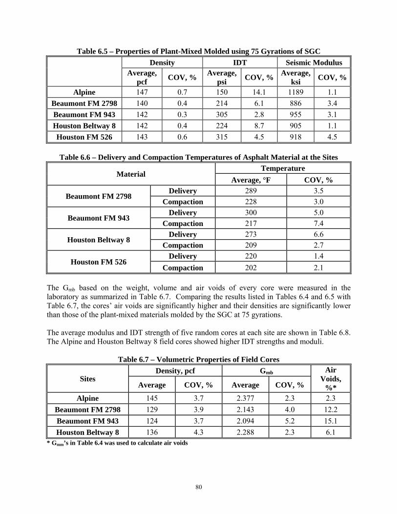
80
Table 6.5 – Properties of Plant-Mixed Molded using 75 Gyrations of SGC
Density IDT Seismic Modulus
Average, pcf
COV, % Average,
psi COV, %
Average, ksi
COV, %
Alpine 147 0.7 150 14.1 1189 1.1
Beaumont FM 2798 140 0.4 214 6.1 886 3.4
Beaumont FM 943 142 0.3 305 2.8 955 3.1
Houston Beltway 8 142 0.4 224 8.7 905 1.1
Houston FM 526 143 0.6 315 4.5 918 4.5
Table 6.6 – Delivery and Compaction Temperatures of Asphalt Material at the Sites
Material Temperature
Average, °F COV, %
Beaumont FM 2798 Delivery 289 3.5
Compaction 228 3.0
Beaumont FM 943 Delivery 300 5.0
Compaction 217 7.4
Houston Beltway 8 Delivery 273 6.6
Compaction 209 2.7
Houston FM 526 Delivery 220 1.4
Compaction 202 2.1
The Gmb based on the weight, volume and air voids of every core were measured in the laboratory as summarized in Table 6.7. Comparing the results listed in Tables 6.4 and 6.5 with Table 6.7, the cores’ air voids are significantly higher and their densities are significantly lower than those of the plant-mixed materials molded by the SGC at 75 gyrations. The average modulus and IDT strength of five random cores at each site are shown in Table 6.8. The Alpine and Houston Beltway 8 field cores showed higher IDT strengths and moduli.
Table 6.7 – Volumetric Properties of Field Cores
Sites Density, pcf Gmb Air
Voids, %* Average COV, % Average COV, %
Alpine 145 3.7 2.377 2.3 2.3
Beaumont FM 2798 129 3.9 2.143 4.0 12.2
Beaumont FM 943 124 3.7 2.094 5.2 15.1
Houston Beltway 8 136 4.3 2.288 2.3 6.1 * Gmm’s in Table 6.4 was used to calculate air voids
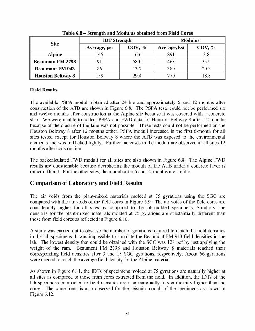
81
Table 6.8 – Strength and Modulus obtained from Field Cores
Site IDT Strength Modulus
Average, psi COV, % Average, ksi COV, %
Alpine 145 16.6 891 8.8
Beaumont FM 2798 91 58.0 463 35.9
Beaumont FM 943 86 13.7 380 20.3
Houston Beltway 8 159 29.4 770 18.8
Field Results The available PSPA moduli obtained after 24 hrs and approximately 6 and 12 months after construction of the ATB are shown in Figure 6.8. The PSPA tests could not be performed six and twelve months after construction at the Alpine site because it was covered with a concrete slab. We were unable to collect PSPA and FWD data for Houston Beltway 8 after 12 months because of the closure of the lane was not possible. These tests could not be performed on the Houston Beltway 8 after 12 months either. PSPA moduli increased in the first 6-month for all sites tested except for Houston Beltway 8 where the ATB was exposed to the environmental elements and was trafficked lightly. Further increases in the moduli are observed at all sites 12 months after construction. The backcalculated FWD moduli for all sites are also shown in Figure 6.8. The Alpine FWD results are questionable because deciphering the moduli of the ATB under a concrete layer is rather difficult. For the other sites, the moduli after 6 and 12 months are similar.
Comparison of Laboratory and Field Results The air voids from the plant-mixed materials molded at 75 gyrations using the SGC are compared with the air voids of the field cores in Figure 6.9. The air voids of the field cores are considerably higher for all sites as compared to the lab-molded specimens. Similarly, the densities for the plant-mixed materials molded at 75 gyrations are substantially different than those from field cores as reflected in Figure 6.10. A study was carried out to observe the number of gyrations required to match the field densities in the lab specimens. It was impossible to simulate the Beaumont FM 943 field densities in the lab. The lowest density that could be obtained with the SGC was 128 pcf by just applying the weight of the ram. Beaumont FM 2798 and Houston Beltway 8 materials reached their corresponding field densities after 3 and 15 SGC gyrations, respectively. About 66 gyrations were needed to reach the average field density for the Alpine material. As shown in Figure 6.11, the IDTs of specimens molded at 75 gyrations are naturally higher at all sites as compared to those from cores extracted from the field. In addition, the IDTs of the lab specimens compacted to field densities are also marginally to significantly higher than the cores. The same trend is also observed for the seismic moduli of the specimens as shown in Figure 6.12.

82
Figure 6.8 - PSPA and FWD from ATB Sites.
.
430
582
516
385 44
7
687
463 51
4 582
700
720
750
0
100
200
300
400
500
600
700
800
El PasoAlpine
HoustonFM 526
HoustonBeltway 8
BeaumontFM 2798
BeaumontFM 943
Mod
ulu
s, k
si
After 24 hrs After 6 Months After 12 Months
a) PSPA
782
598
597
357
364
614
307 35
3
0100200300400500600700800900
1000
El PasoAlpine
HoustonFM 526
HoustonBeltway 8
BeaumontFM 2798
BeaumontFM 943
Mod
ulu
s, k
si
After 6 Months After 12 Months
b) FWD
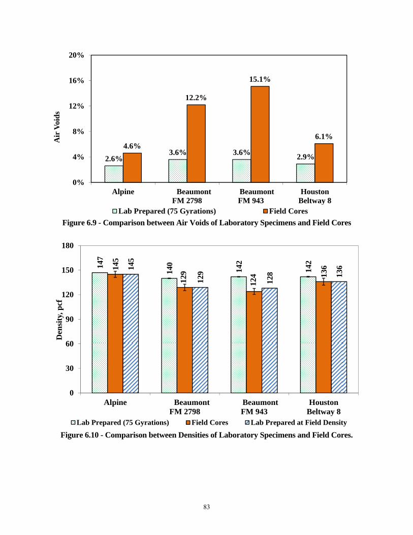
83
Figure 6.9 - Comparison between Air Voids of Laboratory Specimens and Field Cores
Figure 6.10 - Comparison between Densities of Laboratory Specimens and Field Cores.
2.6%3.6% 3.6%
2.9%4.6%
12.2%
15.1%
6.1%
0%
4%
8%
12%
16%
20%
Alpine BeaumontFM 2798
BeaumontFM 943
HoustonBeltway 8
Air
Voi
ds
.
Lab Prepared (75 Gyrations) Field Cores
147
140
142
142
145
129
124 13
6145
129
128 13
6
0
30
60
90
120
150
180
Alpine BeaumontFM 2798
BeaumontFM 943
HoustonBeltway 8
Den
sity
, pcf
Lab Prepared (75 Gyrations) Field Cores Lab Prepared at Field Density
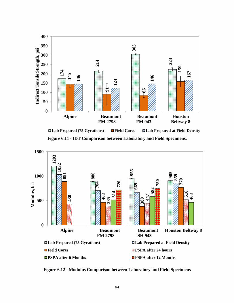
84
Figure 6.11 - IDT Comparison between Laboratory and Field Specimens.
Figure 6.12 - Modulus Comparison between Laboratory and Field Specimens
174
214
305
224
145
91 86
159
146
124 14
6 167
0
50
100
150
200
250
300
350
400
Alpine BeaumontFM 2798
BeaumontFM 943
HoustonBeltway 8
Ind
irec
t T
ensi
le S
tren
gth
, psi
.
Lab Prepared (75 Gyrations) Field Cores Lab Prepared at Field Density
1203
886 95
5
90510
32
704
669
859
891
463
380
770
430
385 44
7 516
514 58
2
463
720
750
0
500
1000
1500
Alpine BeaumontFM 2798
BeaumontSH 943
Houston Beltway 8
Mod
ulu
s, k
si
Lab Prepared (75 Gyrations) Lab Prepared at Field Density
Field Cores PSPA after 24 hours
PSPA after 6 Months PSPA after 12 Months
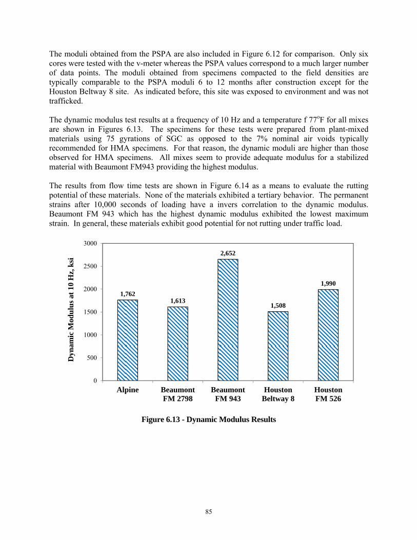
85
The moduli obtained from the PSPA are also included in Figure 6.12 for comparison. Only six cores were tested with the v-meter whereas the PSPA values correspond to a much larger number of data points. The moduli obtained from specimens compacted to the field densities are typically comparable to the PSPA moduli 6 to 12 months after construction except for the Houston Beltway 8 site. As indicated before, this site was exposed to environment and was not trafficked. The dynamic modulus test results at a frequency of 10 Hz and a temperature f 77oF for all mixes are shown in Figures 6.13. The specimens for these tests were prepared from plant-mixed materials using 75 gyrations of SGC as opposed to the 7% nominal air voids typically recommended for HMA specimens. For that reason, the dynamic moduli are higher than those observed for HMA specimens. All mixes seem to provide adequate modulus for a stabilized material with Beaumont FM943 providing the highest modulus. The results from flow time tests are shown in Figure 6.14 as a means to evaluate the rutting potential of these materials. None of the materials exhibited a tertiary behavior. The permanent strains after 10,000 seconds of loading have a invers correlation to the dynamic modulus. Beaumont FM 943 which has the highest dynamic modulus exhibited the lowest maximum strain. In general, these materials exhibit good potential for not rutting under traffic load.
Figure 6.13 - Dynamic Modulus Results
1,7621,613
2,652
1,508
1,990
0
500
1000
1500
2000
2500
3000
Alpine BeaumontFM 2798
BeaumontFM 943
HoustonBeltway 8
HoustonFM 526
Dyn
amic
Mod
ulu
s at
10
Hz,
ksi
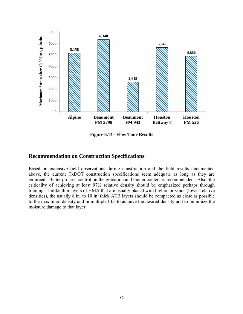
86
Figure 6.14 - Flow Time Results
Recommendation on Construction Specifications Based on extensive field observations during construction and the field results documented above, the current TxDOT construction specifications seem adequate as long as they are enforced. Better process control on the gradation and binder content is recommended. Also, the criticality of achieving at least 97% relative density should be emphasized perhaps through training. Unlike thin layers of HMA that are usually placed with higher air voids (lower relative densities), the usually 8 in. to 10 in. thick ATB layers should be compacted as close as possible to the maximum density and in multiple lifts to achieve the desired density and to minimize the moisture damage to that layer.
5,158
6,340
2,619
5,642
4,880
0
1000
2000
3000
4000
5000
6000
7000
Alpine BeaumontFM 2798
BeaumontFM 943
HoustonBeltway 8
HoustonFM 526
Max
imu
m S
trai
n a
fter
10,
000
sec,
µ-i
n./i
n.
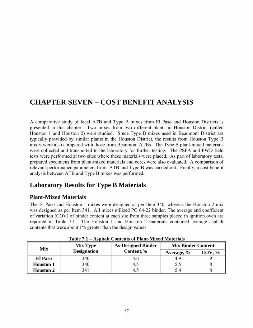
87
CHAPTER SEVEN – COST BENEFIT ANALYSIS A comparative study of local ATB and Type B mixes from El Paso and Houston Districts is presented in this chapter. Two mixes from two different plants in Houston District (called Houston 1 and Houston 2) were studied. Since Type B mixes used in Beaumont District are typically provided by similar plants in the Houston District, the results from Houston Type B mixes were also compared with those from Beaumont ATBs. The Type B plant-mixed materials were collected and transported to the laboratory for further testing. The PSPA and FWD field tests were performed at two sites where these materials were placed. As part of laboratory tests, prepared specimens from plant-mixed materials and cores were also evaluated. A comparison of relevant performance parameters from ATB and Type B was carried out. Finally, a cost benefit analysis between ATB and Type B mixes was performed.
Laboratory Results for Type B Materials
Plant-Mixed Materials The El Paso and Houston 1 mixes were designed as per Item 340, whereas the Houston 2 mix was designed as per Item 341. All mixes utilized PG 64-22 binder. The average and coefficient of variation (COV) of binder content at each site from three samples placed in ignition oven are reported in Table 7.1. The Houston 1 and Houston 2 materials contained average asphalt contents that were about 1% greater than the design values.
Table 7.1 – Asphalt Contents of Plant-Mixed Materials
Mix Mix Type
Designation As-Designed Binder
Content,% Mix Binder Content
Average, % COV, % El Paso 340 4.6 4.9 9
Houston 1 340 4.5 5.5 8 Houston 2 341 4.5 5.4 8
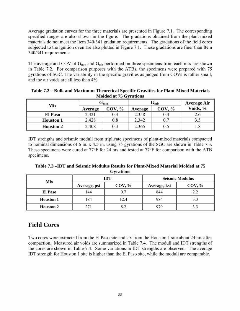
88
Average gradation curves for the three materials are presented in Figure 7.1. The corresponding specified ranges are also shown in the figure. The gradations obtained from the plant-mixed materials do not meet the Item 340/341 gradation requirements. The gradations of the field cores subjected to the ignition oven are also plotted in Figure 7.1. These gradations are finer than Item 340/341 requirements. The average and COV of Gmm and Gmb performed on three specimens from each mix are shown in Table 7.2. For comparison purposes with the ATBs, the specimens were prepared with 75 gyrations of SGC. The variability in the specific gravities as judged from COVs is rather small, and the air voids are all less than 4%.
Table 7.2 – Bulk and Maximum Theoretical Specific Gravities for Plant-Mixed Materials
Molded at 75 Gyrations
Mix Gmm Gmb Average Air
Voids, % Average COV, % Average COV, % El Paso 2.421 0.3 2.358 0.3 2.6
Houston 1 2.428 0.8 2.342 0.7 3.5 Houston 2 2.408 0.3 2.365 0.5 1.8
IDT strengths and seismic moduli from triplicate specimens of plant-mixed materials compacted to nominal dimensions of 6 in. x 4.5 in. using 75 gyrations of the SGC are shown in Table 7.3. These specimens were cured at 77°F for 24 hrs and tested at 77°F for comparison with the ATB specimens.
Table 7.3 –IDT and Seismic Modulus Results for Plant-Mixed Material Molded at 75 Gyrations
Mix IDT Seismic Modulus
Average, psi COV, % Average, ksi COV, %
El Paso 144 0.7 844 2.2
Houston 1 184 12.4 984 3.3
Houston 2 271 8.2 979 3.3
Field Cores Two cores were extracted from the El Paso site and six from the Houston 1 site about 24 hrs after compaction. Measured air voids are summarized in Table 7.4. The moduli and IDT strengths of the cores are shown in Table 7.4. Some variations in IDT strengths are observed. The average IDT strength for Houston 1 site is higher than the El Paso site, while the moduli are comparable.
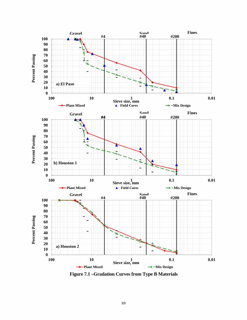
89
Figure 7.1 –Gradation Curves from Type B Materials
0102030405060708090
100
0.010.1110100
Per
cen
t P
assi
ng
Sieve size, mmPlant Mixed Field Cores Mix Design
#4 #40 #200Gravel Sand Fines
a) El Paso
0102030405060708090
100
0.010.1110100
Per
cent
Pas
sing
Sieve size, mmPlant Mixed Field Cores Mix Design
#4 #40 #200Gravel Sand Fines
b) Houston 1
#4
0102030405060708090
100
0.010.1110100
Per
cen
t P
assi
ng
Sieve size, mmPlant Mixed Mix Design
#4 #40 #200Gravel Sand Fines
a) Houston 2
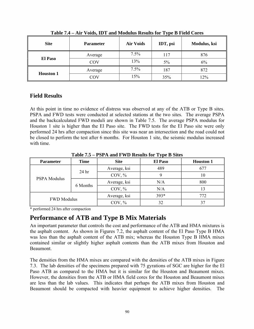
90
Table 7.4 – Air Voids, IDT and Modulus Results for Type B Field Cores
Site Parameter Air Voids IDT, psi Modulus, ksi
El Paso Average 7.5% 117 876
COV 13% 5% 6%
Houston 1 Average 7.5% 187 872
COV 15% 35% 12%
Field Results At this point in time no evidence of distress was observed at any of the ATB or Type B sites. PSPA and FWD tests were conducted at selected stations at the two sites. The average PSPA and the backcalculated FWD moduli are shown in Table 7.5. The average PSPA modulus for Houston 1 site is higher than the El Paso site. The FWD tests for the El Paso site were only performed 24 hrs after compaction since this site was near an intersection and the road could not be closed to perform the test after 6 months. For Houston 1 site, the seismic modulus increased with time.
Table 7.5 – PSPA and FWD Results for Type B Sites Parameter Time Site El Paso Houston 1
PSPA Modulus
24 hr Average, ksi 489 677
COV, % 9 10
6 Months Average, ksi N/A 800
COV, % N/A 13
FWD Modulus Average, ksi 393* 772
COV, % 32 37 * performed 24 hrs after compaction
Performance of ATB and Type B Mix Materials An important parameter that controls the cost and performance of the ATB and HMA mixtures is the asphalt content. As shown in Figures 7.2, the asphalt content of the El Paso Type B HMA was less than the asphalt content of the ATB mix; whereas the Houston Type B HMA mixes contained similar or slightly higher asphalt contents than the ATB mixes from Houston and Beaumont. The densities from the HMA mixes are compared with the densities of the ATB mixes in Figure 7.3. The lab densities of the specimens prepared with 75 gyrations of SGC are higher for the El Paso ATB as compared to the HMA but it is similar for the Houston and Beaumont mixes. However, the densities from the ATB or HMA field cores for the Houston and Beaumont mixes are less than the lab values. This indicates that perhaps the ATB mixes from Houston and Beaumont should be compacted with heavier equipment to achieve higher densities. The

91
densities for the HMA mixes are reasonable given the current TxDOT specification requiring approximately 8% air voids.
Figure 7.2 – Comparison of Asphalt Content for ATB and Type B Specimens
Figure 7.3 – Comparison of Density for ATB and Type B Specimens
4.6
6.0
4.5
5.4
4.54.1 4.1
4.8
5.55.0
4.64.3
4.8
0
1
2
3
4
5
6
7
Type B ATB Type B Type B ATB ATB ATB
El Paso Alpine Houston 1 Houston 2 Beltway 8 FM 2798 FM 943
Asp
hal
t C
onte
nt, %
Plant-Mixed Materials Field CoresEl Paso Houston Beaumont
140
147
141143 142
140142142
145
133136
129
124
100
110
120
130
140
150
160
Type B ATB Type B Type B ATB ATB ATB
El Paso Alpine Houston 1 Houston 2 Beltway 8 FM 2798 FM 943
Den
sity
, pcf
Plant-Mixed Materials Field CoresEl Paso Houston Beaumont

92
Figure 7.4 shows the IDT strengths for all materials and mix types. For El Paso materials; the lab-prepared Type B and ATB specimens exhibited similar IDT strengths but the field cores are stronger for the ATB mix as compared to the Type B mix. The trends of the IDT strengths of the lab-prepared specimens for Type B and ATB mixes from Houston/Beaumont are mixed. However, the IDT strengths of the cores from Type B are greater than those from the ATB’s for the Houston/Beaumont mixes.
Figure 7.4 – Comparison of Indirect Tensile Strength for ATB and Type B Specimens
The stiffness properties of the mixes were assessed using the dynamic modulus and flow time tests. The results between these two mixes are compared in Figures 7.5 and 7.6. The Type B and ATB mixes for El Paso exhibited similar values for both tests. However, the two Type B mixes from Houston seem to perform better than the ATB mixes except in one case. To quantify moisture susceptibility of mixes, tests were conducted using the Hamburg Wheel-Tracking device (HWTD) according to Tex-242-F. Testing was performed on plant-mixed specimens using 75 gyrations of the SGC. The results from the HWTD are summarized in Table 7.6. Even though the minimum number of passes required for a PG 64-22 binder is 10,000, tests were conducted to 20,000 passes. All materials tested exhibited acceptable rut depths at all cycles. The variations in the field moduli measured with the PSPA and FWD are shown in Figure 7.7. The moduli of the Type B mixes 24 hrs after construction are greater than the ATBs perhaps because of better quality control and the fact that the HMAs were placed in thinner lifts. The PSPA moduli increase with time for most ATB sites except one site that was exposed to elements. Similar trends are observed from the FWD results.
144
150
184
270
224
214
305
117 14
5
187
159
91 86
0
50
100
150
200
250
300
350
Type B ATB Type B Type B ATB ATB ATB
El Paso Alpine Houston 1 Houston 2 Beltway 8 FM 2798 FM 943
Ind
irec
t Ten
sile
Str
engt
h, p
si
Plant-Mixed Materials Field CoresEl Paso Houston Beaumont
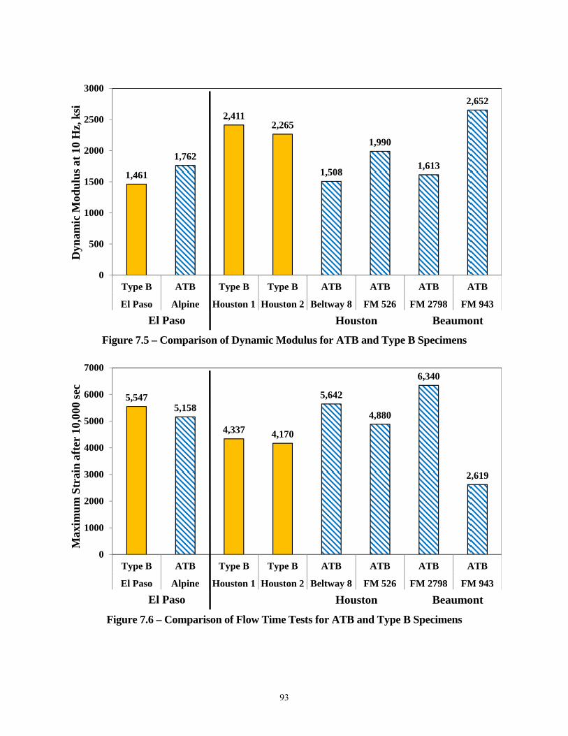
93
Figure 7.5 – Comparison of Dynamic Modulus for ATB and Type B Specimens
Figure 7.6 – Comparison of Flow Time Tests for ATB and Type B Specimens
1,461
1,762
2,4112,265
1,508
1,990
1,613
2,652
0
500
1000
1500
2000
2500
3000
Type B ATB Type B Type B ATB ATB ATB ATB
El Paso Alpine Houston 1 Houston 2 Beltway 8 FM 526 FM 2798 FM 943
Dyn
amic
Mod
ulus
at
10 H
z, k
si
El Paso Houston Beaumont
5,5475,158
4,337 4,170
5,642
4,880
6,340
2,619
0
1000
2000
3000
4000
5000
6000
7000
Type B ATB Type B Type B ATB ATB ATB ATB
El Paso Alpine Houston 1 Houston 2 Beltway 8 FM 526 FM 2798 FM 943
Max
imu
m S
trai
n af
ter
10,0
00 s
ec
El Paso Houston Beaumont
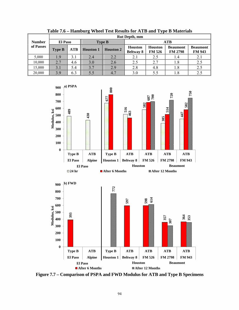
94
Table 7.6 – Hamburg Wheel Test Results for ATB and Type B Materials
Number of Passes
Rut Depth, mm El Paso Type B ATB
Type B ATB Houston 1 Houston 2 Houston
Beltway 8 Houston FM 526
Beaumont FM 2798
Beaumont FM 943
5,000 1.9 3.1 2.4 2.2 2.1 2.5 1.4 2.1 10,000 2.7 4.6 3.0 2.6 2.5 2.7 1.8 2.5 15,000 3.1 5.4 3.7 2.9 2.8 4.8 1.8 2.5 20,000 3.9 6.3 5.5 4.7 3.0 5.5 1.8 2.5
Figure 7.7 – Comparison of PSPA and FWD Modulus for ATB and Type B Specimens
393
597
598
357
364
772
614
307 35
3
0
100
200
300
400
500
600
700
800
900
Type B ATB Type B ATB ATB ATB ATB
El Paso Alpine Houston 1 Beltway 8 FM 526 FM 2798 FM 943
Mod
ulu
s, k
si
After 6 Months After 12 Months
b) FWD
Houston BeaumontEl Paso
489
430
677
516 58
2
385 44
7
800
463
687
514 58
2
700
720 75
0
0
100
200
300
400
500
600
700
800
900
Type B ATB Type B ATB ATB ATB ATB
El Paso Alpine Houston 1 Beltway 8 FM 526 FM 2798 FM 943
Mod
ulu
s, k
si
24 hr After 6 Months After 12 Months
a) PSPA
Houston BeaumontEl Paso
95
Cost Comparison A cost comparison was performed using TxDOT program Letting V9. This program reflects what TxDOT pays for each material including the cost of the raw material, asphalt binder, transportation from plant to the site and construction. Figure 7.8 compares on a yearly basis the usage and price per ton of Type B and ATB in Beaumont/Houston area. The study was focused on these two districts because they place more than 90% of the ATB’s in Texas. For these two districts, the average unit price of the ATB is less than the Type B mixes. However, as reflected in Figure 7.8a, Type B mixes are not very popular in that region. For a more equitable cost analysis, the state-wide weighted average cost per ton of Type B mixes is also included in Figure 7.8b. The state-wide unit costs of Type B mixes are comparable with the unit costs of ATBs from Houston/Beaumont area. These trends indicate that the cost of the ATB mix will be comparable to the Type B mixes, should other districts in Texas decide to place higher quantities of ATB. Figure 7.9 compares the costs of the specific ATB and Type B mixes studied in this chapter. Since El Paso District hardly ever uses the ATB mixes, its unit cost is significantly greater than the comparable Type B mix. This trend reverses for the Houston/Beaumont area where the ATB is used substantially more frequently than the Type B. This case study demonstrates that the unit cost of the ATB will be comparable or less expensive than the Type B mixes, if the districts decide to use the ATB based on the perceived more reasonable and convenient new mix design process.
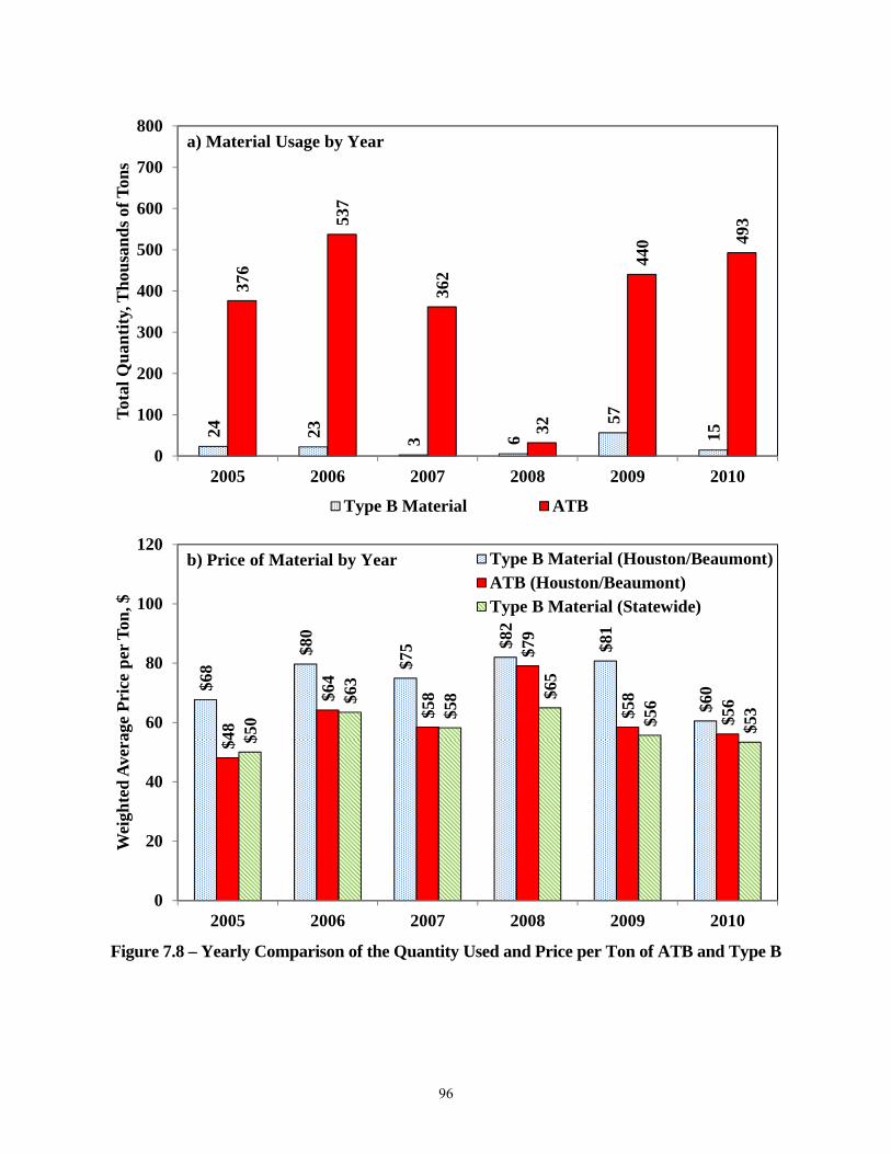
96
Figure 7.8 – Yearly Comparison of the Quantity Used and Price per Ton of ATB and Type B
24 23 3 6
57
15
376
537
362
32
440 49
3
0
100
200
300
400
500
600
700
800
2005 2006 2007 2008 2009 2010
Tot
al Q
uan
tity
, Th
ousa
nd
s of
Ton
s
Type B Material ATB
a) Material Usage by Year
$68
$80
$75 $8
2
$81
$60
$48
$64
$58
$79
$58
$56
$50
$63
$58 $6
5
$56
$53
0
20
40
60
80
100
120
2005 2006 2007 2008 2009 2010
Wei
ghte
d A
vera
ge P
rice
per
Ton
, $
Type B Material (Houston/Beaumont)ATB (Houston/Beaumont)Type B Material (Statewide)
b) Price of Material by Year

97
Figure 7.9 – Comparison of Price per Ton of ATB and Type B by Site
$54
$66
$105
$87
$48
$64
$0
$20
$40
$60
$80
$100
$120
El Paso Beaumont Houston
Pri
ce p
er T
on, $
Type B Material ATB
StandardDeviation
15

98
99
CHAPTER EIGHT – CLOSURE Asphalt treated bases (ATBs) in Texas are usually designed and constructed as per Item 292, “Asphalt Treatment (Plant Mixed),” of the 2004 Standard Specification book. This specification is a hybrid of base and hot mix asphalt concrete procedures and requirements, which are sometimes incompatible. In addition, this Item uses a specific Texas Gyratory Base Compactor that is not readily available to all districts. The objective of this project was to propose a new mix design procedure for asphalt-treated bases that can use standard equipment such as the Superpave Gyratory Compactor (SGC) to mold the specimens for mix design. To achieve the objective of this project, current TxDOT procedures such as Tex-126-E and Tex-204-F were evaluated and modified to propose new generically-named Tex-126-H and Tex-204-H test. A comprehensive parametric study comparing the results of the two proposed procedures with the existing procedures was performed. The most practical setup for laboratory tests was achieved by using Tex-204-H procedures, which proposes preparation of 6 in. diameter and 4.5 in. high specimens using 75 gyrations with the SGC. Furthermore, it is recommended to cure specimens for 24 hrs at room temperature (77°F) before conducting the indirect tensile strength because the results from this procedure were more sensitive to asphalt content while reducing the mix design period. The appropriate asphalt content should satisfy a target indirect tensile strength of at least 85 psi, and a relative density of 97%. A cost-benefit analysis was also carried out between the ATB and Type B HMA. It seems that in most cases, the performance of the ATB mixes is comparable or slightly inferior to the Type B mixes. The main benefits of the ATB over HMA are that the local materials can be potentially used and that the ATB mixes are less permeable than the Type B mixes. The cost seems to be dictated by the popularity of mixes in given districts. The average unit cost of the ATB is less than Type B in the Houston/Beaumont area because the ATB is used more extensively than Type B. However, the average state-wide unit costs of the Type B are comparable to the ATB. Based on the overall results of this study, the following conclusions can be outlined: The Superpave Gyratory Compactor results were found to be more uniform and consistent
compared to the Texas Gyratory Base Compactor. Specimens prepared with the Superpave Gyratory Compactor usually exhibit similar or
higher unconfined compressive strength and indirect tensile strengths as compared to those prepared with the Texas Gyratory Base Compactor.
The indirect tensile strength was found to be more sensitive to the asphalt content, so it was selected to be as a parameter to estimate the optimum moisture content for a mix design.

100
Curing of specimens at 77°F (room temperature) for 24 hrs after compaction did not yield strengths that were statistically different than curing the specimens at higher temperatures longer duration provided the specimens are tested at a temperature of 77°F.
The optimum asphalt content obtained following the newly-proposed protocol is higher than those from traditional Item 292.
Specimens molded with 80 gyrations were found to have the highest sensitivity to asphalt content as compared to the specimens molded at 60 and 100 gyrations. Since the 75 gyrations are already included in some of the procedures in Tex-204-F, 75 was selected as the number of gyrations.
Unlike the traditional HMA mixes that are placed at air voids of about 8%, the ATB should be compacted to a relative density of 97% or greater to realize its benefits. Since the ATBs are placed in thicker lifts, heavier compactors may be necessary.
101
REFERENCE 1. AASHTO, Designation T269, “Percent Air Voids in Compacted Dense and Open Asphalt
Mixtures” Standard Specifications for Transportation Materials and Methods of Sampling and Testing, 25th Edition, AASHTO, Washington, DC, 2005, CD-ROM.
2. Aguiar-Moya, J. P., Prozzi, J. A., Tahmoressi, M. “Optimum Number of Superpave Gyrations Based on Project Requirements”. Transportation Research Board, Washington D.C. 2007
3. Azari, H., Lutz, R., and Spellberg, P., “Precision Estimates of Selected Volumetric Properties of HMA Using Absorptive Aggregate,” Submitted for Approval by the NCHRP 9-26 Panel. 2006
4. Azari, H., Lutz, R., And Spellberg, P., “Precision Estimates for AASHTO Test Method T 269 Determined Using AMRL Proficiency Sample Data,” NCHRP Web Document 114, 2007
5. Button, J. W., Chowdhury, A., and Bhasin A. (2006) “Transitioning from the Texas Gyratory Base Compactor to the Superpave Gyratory Compactor” 86th Annual Meeting of the Transportation Research Board, Washington, D.C., January 2006
6. Button, J. W., Little, D.N., Jagadam, V., and Pendleton, O.J. “correlation of Selected Laboratory Compaction Methods with Field Compaction,” Transportation Research Record 1454, Transportation Research Board, Washington D.C., 1994, pp. 193-201
7. Chakroborty, P., and Das, A. Principles of Transportation Engineering PHI Learning Pvt. Ltd., pp 360. 2004
8. Cedergren, H.R. Drainage of Highway and Airfield Pavements, John Wiley & Sons, New York. 1977.
9. Collins, R., Watson, D., Johnson, A., and Wu, Y. Effect of Aggregate Degradation of Specimens Compacted by Superpave Gyratory Compactor. In Transportation Research Record: Journal of the Transportation Research Board, No. 1590, TRB, National Research Council, Washington D.C., 1997, pp.1-9
10. Dykman, M., Ramanujam, J.M., and Nataatmadja, A. (2003) “Performance of Bitumen Treated Bases” 82nd Annual Meeting of the Transportation Research Board, Washington, D.C., January 2003
11. Harman, T., Bukowski, J.R., Mountier, F., Huber, G., and McGennis, R. “The History and Future Challenges Of Gyratory Compaction 1939 to 2001,” Transportation Research Board, National Research council, Washington, D.C., 2002
12. Holsinger, R.E., Fisher, A., and Spellberg, P.A., “Precision Estimates for AASHTO Test Method T308 and the Test Methods for Performance-Graded Asphalt Binder in AASHTO Specification M320,” NCHRP Web Document 71, 2005

102
13. Marks, V.J. and Huisman, C.L. Reducing the Adverse Effects of Transverse Cracking, Transportation Research Record, 1034, pp 80-86. 1985
14. McDowell, C., and Smith, A.W. “Design, Control, and Interpretation of Tests for Bituminous Hot Mix Black Base Mixtures”. Materials and Test Division, Soils Section Texas Highway Department, 1969
15. Mokwa, R., Cuelho, E., Browne, M. “Laboratory Testing of Soils Using the Superpave Gyratory Compactor” 87th Annual Meeting of the Transportation Research Board, Washington, D.C., January 2008
16. Peterson, R. L., Mahboub, K. C., Anderson, R. M., Masad, E., Tashman, T. Comparing Superpave Gyratory Compactor Data to Field Cores. Journal of Materials in Civil Engineering ASCE. 2004
17. Saeed A., Hall, J.W., and Barker W., “Performance-Related Tests of Aggregates for Use in Unbound Pavement Layers,” NCHRP Report 453, national Academy of Engineering, Washington, DC. 2001
18. Sebesta, S., Guthrie, W.S., and Harris, J.P. “Gyratory Compaction of Soils for Laboratory Swell Tests,” Proceedings; 83rd Annual Meeting of the Transportation Research Board, Washington, D.C., January 2004
19. Spellberg, P.A., and Savage, D.A., “An Investigation of the Cause of Variation in HMA Bulk Specific Gravity Test Results Using Non-Absorptive Aggregates,” NCHRP Web Document 66, 2004
20. Spellberg, P.A., Savage, D.A., and Pielert, J.H., “Precision Estimates of Selected Volumetric Properties of HMA Using Non-Absorptive Aggregate” NCHRP Web Document 54, 2003
21. Ullman & Nolan Consulting Engineers. Report on Design Characteristic for Logan City Council. Reference 1419U\PJD\8.91.1991
22. Varvik, W. R., and S. H. Carpenter, “Calculating Air Voids at Specified Numbers of Gyrations in Superpave Gyratory Compactor,” Transportation Research Record 1630, 1998.
23. Von Quintus, H., Scherocman, J.A., Hughes, C.W., and Kennedy, T.W. “Asphalt-Aggregate Mixture Analysis System –AAMAS,” NCHRP Report 338, national cooperative Highway Research Program, Transportation Research Board, Washington, D.C., 1991
24. Wong, W.G., Yang, Q., and Wang, K.C.P. “Performance-Based Mixture Design of Asphalt-Treated Base,” Journal of the Institution of Engineers, Vol. 44 Issue 2, Singapore. 2004

103
Appendix A
Questionnaire

104
105
Questionnaire for TxDOT Research Project 0-6361 Development of a New Mix Design Method and Specification Requirements for Asphalt
Treated Base (Item 292) The asphalt stabilized bases in Texas are traditionally designed and constructed as per Item 292, “Asphalt Treatment (Plant Mixed),” of the 2004 Standard Specification book. Due to scarcity of the appropriate compactor specified in Item 292, some districts have started using Tex-204-F, Part III, ‘Mix Design for Large Stone Mixtures Using the Superpave Gyratory Compactor.” A new mix design procedure is needed for this type of material that can use standard equipment such as the Superpave Gyratory Compactor (SGC) to mold the mix design specimens.
UTEP has been granted a research project to evaluate Item 292 and to improve the laboratory design protocols for this type of base. The research team will also concentrate on the practical issues of the construction including the quality control and quality assurance and what test should be used to control the quality in the field.
This questionnaire is the first step toward documenting the current practices of TxDOT in using ATB. Your response to this questionnaire will help the research team to focus their efforts to provide a more practical and useful final product.

106
Questionnaire for TxDOT Research Project 0-6361 District: _________________ Contact Person(s): ___________________________________ Telephone numbers and e-mails of contact persons: ______________________________________________________________________________ (1) Have you used or are you using asphalt treated base (ATB) in construction/rehabilitation
projects in your district? Yes No (2) If yes, how many such projects have been completed in the last 5 years or are scheduled to
be constructed in the near future in your district? ______ projects
(3) Which specification do you use for the design of ATB?
Item 292 Tex-204-F Part III Both Others (specify) _________
If you use Item 292 or Tex-204-F Part III, do you waive any of the requirements? (If yes, please indicate them below)
(4) Which compactor do you use for the design of ATB?
Texas Gyratory Superpave Gyratory Both Others (specify) _____________ (5) What are the main uses of the ATB in your district? (check as many as apply to your district) Alternative to unbound base Alternative to stabilized base Alternative to Type A/B HMA Alternative to bond breaker layer under PCC Others (please specify) ____________________________________ (6) What factors motivate you to select ATB for projects in your district over other alternatives
named in Question 3? (Please check as many as apply and comment in front of each line). more economical____________________________________________________
lack of appropriate aggregates for alternatives_____________________________
easier to construct __________________________________________________
easier to incorporate recycled materials __________________________________
Others (please specify) _______________________________________________
________________________________________________________________________

107
(7) What typical aggregate types does your district use on ATB projects?
Limestone Sandstone Granite Others (specify) ____________________
(8) Do you add RAP or Crushed Concrete to your ATB? RAP Crushed Concrete Both Neither
(9) As per Item 292, what are the major types and grades of the materials you use in your
district? Please fill out the table below (assign a 1 for the ones you most use, a 2 for the ones you sometime use, and a 3 for those that you rarely use).
Grade Type A Type B
1 2 3
(10) What binder grades does your district use on ATB projects?
________________________________________________________________________ (11) What criteria are used to determine the amounts of binder? Based on district experience Based on existing or special TxDOT specifications (please specify) ___________ Based on vendor’s specifications (please specify) ________________________ (12) What construction specifications do you use for your projects? ________________________________________________________________________ (13) What types of problems, if any, you have encountered with deign or construction of ATB?
________________________________________________________________________ ________________________________________________________________________ ________________________________________________________________________ ________________________________________________________________________ ________________________________________________________________________ (14) Could you please comment on any area that this research should address to help you?
________________________________________________________________________ ________________________________________________________________________ ________________________________________________________________________ ________________________________________________________________________ ________________________________________________________________________ Do you mind if we contact you for more information? Yes No

108
109
Appendix B
Tex-204-H Test Procedure

110
111
112

113

114

115
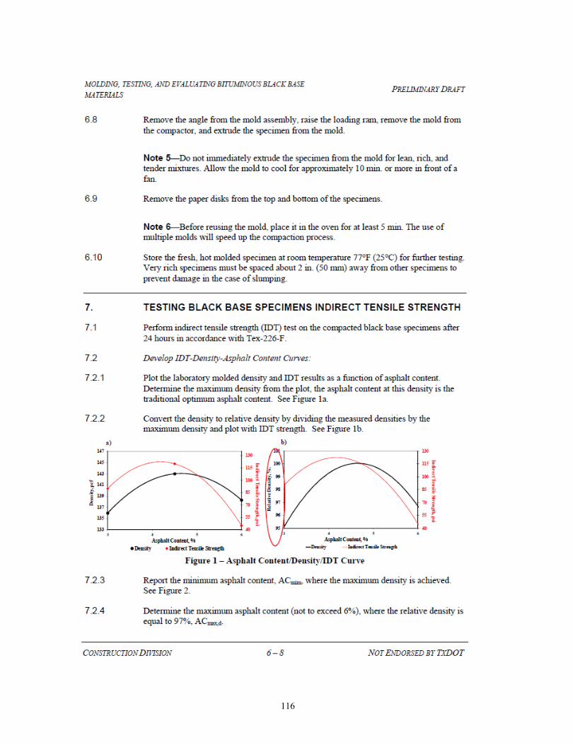
116

117