development of a new methodology for measuring …
TRANSCRIPT
DEVELOPMENT OF A NEW METHODOLOGY FOR
MEASURING DEFORMATION IN TUNNELS AND SHAFTS WITH
TERRESTRIAL LASER SCANNING (LIDAR) USING ELLIPTICAL
FITTING ALGORITHMS
by
Dani Delaloye
A thesis submitted to the Department of Geological Sciences and Geological Engineering
In conformity with the requirements for
the degree of Master of Applied Science
Queen’s University
Kingston, Ontario, Canada
(May, 2012)
Copyright ©Dani Delaloye, 2012
ii
Abstract
Three dimensional laser scanning, also known as Light Detection and Ranging (LiDAR)
has quickly been expanding in its applications in the field of geological engineering due to its
ability to rapidly acquire highly accurate three dimensional positional data. Recently is has been
shown that LiDAR scanning can be easily integrated into an excavation sequence in an
underground environment for the purpose of collecting rockmass and discontinuity information.
As scans are often taken multiple times of the same environment, the next logical application of
LiDAR scanning is for monitoring for change and deformation.
Traditionally, deformation and change in an underground environment is measured using
a series of five or more permanent control points installed around the profile of an excavation.
Using LiDAR for profile analysis provides many benefits as compared to traditional monitoring
techniques. Due to the high density of the point cloud data, the change in profile is able to be
fully characterized, and areas of anomalous movement can easily be separated from overall
closure trends. Furthermore, monitoring with LiDAR does not require the permanent installation
of control points, therefore monitoring can be completed more quickly after excavation, and
scanning is non-invasive therefore no damage is done during the installation of temporary control
points.
The main drawback of using LiDAR scanning for deformation monitoring is that the raw
point accuracy is generally the same magnitude as the smallest level of deformations that need to
be measured. To overcome this, statistical techniques for profile analysis must be developed.
This thesis outlines the development one such method, called the Elliptical Fit Analysis (EFA)
and LiDAR Profile Analysis (EFA) for tunnel and shaft convergence analysis. Testing of the
EFA and LPA has proved the robustness of this technique in its ability to deal with accuracy and
precision issues associated with LiDAR scanning.

iii
Co-Authorship
The thesis “Development of a new methodology for measuring deformation in tunnels
and shafts with terrestrial laser scanning (LiDAR) using elliptical fitting algorithms” is the
product of the formal research of Dani Delaloye. However, the support of Mark Diederichs and
Jean Hutchinson largely helped guide her ideas and writing. Complete references for submitted
journal papers are included in Chapter 7.

iv
Acknowledgements
Many thanks go out to my supervisors, colleagues and friends for their continued support
during the research and publication of this thesis:
To my supervisors, Mark Diederichs and Jean Hutchinson, for their continued guidance.
They pushed me to broaden my knowledge and achieve much more through this thesis than I ever
thought possible.
To Matt Lato, for generously sharing his abundant knowledge of LiDAR. He was a great
mentor, always there to answer my questions and share in my frustrations when questions were
not easily answered.
I also owe thanks to my colleagues within the department involved with LiDAR,
specifically Steph Fekete for her initial instruction in all things LiDAR, Rob Harrap for showing
me how to use all of our equipment and helping me formulate questions at the beginning of my
thesis, and Dave Ball for his software and license assistance.
A huge thank you to the entire Geomechanics Research Group. The group as a whole has
been extremely supportive during the entirely of the past two years. To Anna Crockford, words
cannot explain how lucky I am to have a friend like you. I owe a huge debt to Gabe Walton for
all of the help he provided with developing my Matlab code, and for actually taking the time to
try and understand all the tiny details of my thesis. To Connor Langford, for always offering a
helping hand and listening to my rants about trying to actually create an impact through research.
To Dave Gauthier, Cara Kennedy and Jenn Day for their assistance in the field.
Thank you to NSERC, NWMO, and CEMI for providing funding for the research
conducted during the completion of this thesis.
And finally, thanks to my parents for their continued support throughout all my academic
endeavors.

v
Table of Contents
Abstract ............................................................................................................................................ ii
Co-Authorship ................................................................................................................................ iii
Acknowledgements ......................................................................................................................... iv
Chapter 1 Introduction ..................................................................................................................... 1
1.1 Project motivation and overview .............................................................................. 1
1.2 Thesis format ............................................................................................................ 2
1.3 Synopsis of findings .................................................................................................. 2
1.3.1 Examination of LiDAR accuracy and precision ................................................ 2
1.3.2 Development of technique for tunnel and shaft profile analysis using LiDAR
data ........................................................................................................................................... 3
1.3.3 Testing the sensitivity of the newly developed LiDAR profile analysis
technique .................................................................................................................................. 3
1.3.4 Workflow for tunnel and shaft deformation analysis using LiDAR data .......... 4
1.4 Thesis summary ........................................................................................................ 4
Chapter 2 Background Information and Preliminary Experimentation ........................................... 5
2.1 Preliminary Analysis of LiDAR Application to Change detection ........................... 6
2.2 Scoping analysis of shaft deformation .................................................................... 11
Chapter 3 Development of an Elliptical Fitting Algorithm for Tunnel Deformation Monitoring
with Static Terrestrial LiDAR Scanning ........................................................................................ 17
3.1 Abstract ................................................................................................................... 17
3.2 Introduction ............................................................................................................. 18
3.3 Deformation monitoring in tunnels ......................................................................... 19
3.3.1 Traditional monitoring techniques ................................................................... 21
3.3.2 Georeferencing and absolute positioning ......................................................... 24
3.3.3 Permanent referencing in an active tunneling environment ............................. 25
3.3.4 Back analysis using deformation measurements ............................................. 26
3.4 Accuracy and noise in LiDAR scanning ................................................................. 26
3.4.1 Non scan related noise ..................................................................................... 27
3.5 Terrestrial LiDAR scanning for deformation monitoring in tunnels and shafts ..... 28
3.5.1 Applications of LiDAR scanning in Geological Engineering .......................... 28
3.5.2 Deformation monitoring with LiDAR ............................................................. 29
vi
3.5.3 Previous work in LiDAR scanning for monitoring tunnel deformation .......... 31
3.5.4 Benefits of LiDAR scanning for deformation monitoring ............................... 33
3.5.5 Limitations and errors in current analysis techniques ...................................... 34
3.6 Ellipse fitting for tunnel deformation analysis ........................................................ 36
3.6.1 Methods of ellipse fitting ................................................................................. 38
3.6.1.1 Algebraic ellipse fitting ............................................................................. 38
3.6.1.2 Geometric ellipse fitting ........................................................................... 40
3.7 Tunnel profile analysis with LiDAR ....................................................................... 43
3.7.1 Elliptical Fit Analysis ...................................................................................... 46
3.7.2 LiDAR Profile Analysis ................................................................................... 47
3.7.3 Data filtering .................................................................................................... 52
3.8 Workflow ................................................................................................................ 53
3.9 Application of EFA and LPA to real data ............................................................... 56
3.10 Conclusions ........................................................................................................... 61
Chapter 4 Sensitivity Testing of the Newly Developed Elliptical Fitting Method for the
Measurement of Convergence in Tunnels and Shafts .................................................................... 65
4.1 Abstract ................................................................................................................... 65
4.2 Introduction ............................................................................................................. 66
4.3 Deformation monitoring in tunnels ......................................................................... 66
4.3.1 Traditional monitoring techniques ................................................................... 67
4.4 Terrestrial laser scanning ........................................................................................ 68
4.4.1 Time of flight scanners .................................................................................... 69
4.4.2 Phase shift scanners ......................................................................................... 70
4.5 Sources of error in LiDAR scanning ...................................................................... 71
4.5.1 Sources of range error ...................................................................................... 73
4.5.1.1 Noise created by the scanner ..................................................................... 74
4.5.1.2 Beam divergence and spot size effect ....................................................... 76
4.5.1.3 Surface reflectivity .................................................................................... 78
4.5.1.4 Scan density and spatial resolution ........................................................... 80
4.5.1.5 Angle of incidence .................................................................................... 80
4.5.2 Sources of angular error ................................................................................... 81
4.5.3 Other sources of error ...................................................................................... 82
4.5.3.1 Spurious scan points ................................................................................. 82
vii
4.5.3.2 Ambiguity interval .................................................................................... 82
4.5.3.3 Georeferencing and alignment error ......................................................... 83
4.6 Sources of noise in tunneling .................................................................................. 83
4.7 Positioning in LiDAR scanning .............................................................................. 84
4.8 Tunnel profile analysis with LiDAR data using elliptical fitting ............................ 84
4.8.1 Generating synthetic LiDAR tunnel profiles ................................................... 85
4.8.2 Expected outcomes of EFA and LPA analysis ................................................ 88
4.8.2.1 Radial uniform deformation ...................................................................... 89
4.8.2.2 Elliptical uniform deformation.................................................................. 89
4.8.2.3 Non-uniform deformation ......................................................................... 92
4.9 Sensitivity testing of the EFA and LPA .................................................................. 92
4.9.1 Results of sensitivity testing with synthetic LiDAR data ................................ 96
4.9.2 Implications of occluded data ........................................................................ 100
4.10 Conclusions ......................................................................................................... 100
Chapter 5 A New Workflow for LiDAR Scanning for Change Detection in Tunnels and Caverns
..................................................................................................................................................... 102
5.1 Abstract ................................................................................................................. 102
5.2 Introduction ........................................................................................................... 102
5.3 LiDAR scanning for deformation measurement ................................................... 104
5.3.1 Noise, accuracy and resolution of LiDAR scanning ...................................... 105
5.3.2 Other sources of noise underground .............................................................. 108
5.4 Workflow for tunnel convergence measurement with LiDAR ............................. 109
5.4.1 Data collection ............................................................................................... 110
5.4.1.1 Scan resolution ........................................................................................ 111
5.4.1.2 Scan spacing and locations ..................................................................... 112
5.4.2 Initial data processing .................................................................................... 117
5.4.2.1 Alignment of scans ................................................................................. 117
5.4.2.2 Filtering of data ....................................................................................... 117
5.4.3 Cross section extraction ................................................................................. 119
5.5 Convergence measurement ................................................................................... 119
5.6 Conclusions ........................................................................................................... 123
Chapter 6 General discussion ....................................................................................................... 124
6.1 Discussion ............................................................................................................. 124
viii
6.2 Limitations ............................................................................................................ 124
6.3 Future work ........................................................................................................... 125
Chapter 7 Summary and Conclusions .......................................................................................... 127
7.1 Summary ............................................................................................................... 127
7.2 Contributions ........................................................................................................ 128
7.2.1 Refereed Journal Articles (Submitted) ........................................................... 128
7.2.2 Refereed Conference Papers ...................................................................... 128
7.2.3 Non-refereed Conference Presentations ......................................................... 129
7.2.4 Courses instructed .......................................................................................... 129
7.3 References ............................................................................................................. 129
Appendix A Matlab code for EFA, LPA, NP and synthetic data generation ............................... 137
Appendix B Complete graphical results of sensitivity analysis of EFA and LPA ....................... 171
ix
List of Figures
Figure 2-1: Set of drawers scanned for initial testing of LiDAR point cloud point to point
comparison for change detection (point cloud intensity data shown). ................................ 7
Figure 2-2: Comparison of LiDAR scans to determine the amount of change measured from
shortest distance point to point comparison with: a) the same scan, b) two scans taken at
the same location, c) two scans taken from different locations, and d) two scans taken
from the same location with a drawer opened by 20 mm before the second scan was
taken. ................................................................................................................................... 8
Figure 2-3: Comparison between different scans: a) the same scan compared to itself, showing
there is no error in comparison; b) two separate scans taken from the same location
showing a distribution in the change measured when they are compared; c) two scans
taken from different locations showing a distribution in the change measured when they
are compared; and d) values of the mean and standard deviation (in mm) of change
measured between scans compared to themselves and to each other. ................................ 9
Figure 2-4: Shortest distance point to point comparison of temporal scans taken within a mining
environment where the rockmass was covered with steel screen. Areas where rocks have
moved behind the screen are indicated with arrows. ........................................................ 10
Figure 2-5: Example of shaft deformation model created in Phase 2 (RocScience 2011).
Direction of displacement zone and boundary displacement progression (white arrows
show direction of joint failure and deformation zone progression with increased stress
ratio, black arrows show direction of boundary deformation). ......................................... 12
Figure 2-6: Average displacements for Queenston Shale analyses with no joints dependent upon
the stress ratio, K. ............................................................................................................. 13
Figure 2-7: Normalized minimum and maximum displacements of each rock type for different K
values. ............................................................................................................................... 15
Figure 3-1: Traditional monitoring of tunnel section using control points. Barla’s technique
defines a) the location of points for chainage array measurements, and b) an example of
displacements of array measurements over time (after Barla 2008). In another plot of
tunnel convergence data (after Schubert et al, 2002), absolute displacement vectors of
five control points are shown in: c) cross section to show vertical movement, and d)
longitudinal section to show lateral translation................................................................. 23
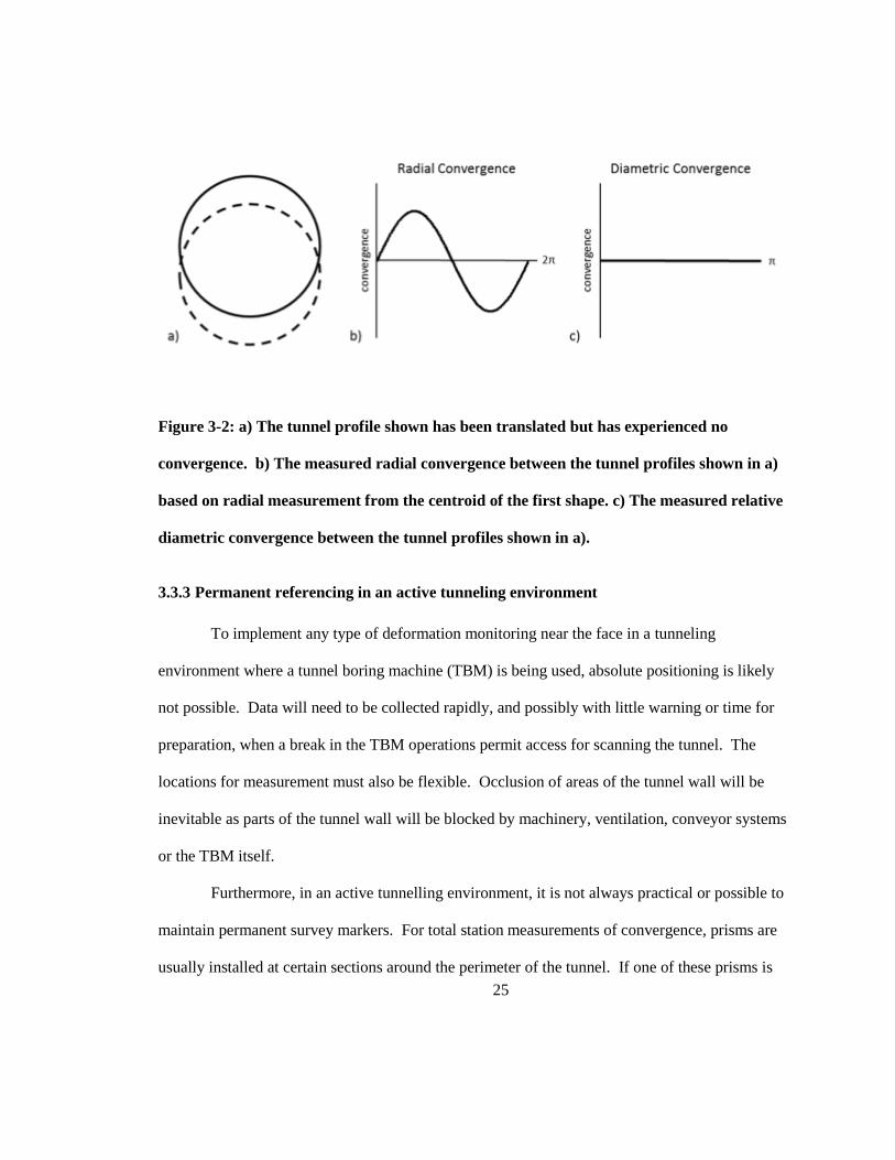
Figure 3-2: a) The tunnel profile shown has been translated but has experienced no convergence.
b) The measured radial convergence between the tunnel profiles shown in a) based on
x
radial measurement from the centroid of the first shape. c) The measured relative
diametric convergence between the tunnel profiles shown in a). ..................................... 25
Figure 3-3: Parameters that characterize an ellipse. The distance that is minimized by a geometric
ellipse fit is the distance between the ith data point (xi, yi) and the corresponding point on
the ellipse (x,y) (after Ray & Srivastava, 2008). ............................................................... 41
Figure 3-4: Example of elliptical fitting for profile analysis: a) two ellipse fits (E1 and E2) with
orientation of long axis displayed, b) distributed radial displacement profile (DRDP)
shown in purple at five times exaggeration, and c) diametric tunnel displacement profile
(DDP). ............................................................................................................................... 48
Figure 3-5: Example of profile analysis with LiDAR point data: a) two LiDAR profiles for
comparison (CS1 in green and CS2 in red), which are elliptically centered, b) distributed
radial displacement profile (DRDP) shown in purple at five times exaggeration, and c)
the diametric tunnel displacement profile (DDP). ............................................................ 50
Figure 3-6: Areas of volume increase and decrease of profile overlain on top of the distributed
radial displacement profile (DRDP) from the LiDAR Profile Analysis (LPA). A positive
volume indicates an area of convergence; a negative value indicates an area of expansion
or divergence. The green line indicates the first LiDAR cross section and the purple line
shows the DRDP. .............................................................................................................. 51
Figure 3-7: Deviation of LiDAR diametric displacement profile from elliptical displacement
profile for characterization of random and systematic noise and anomalous movement of
the tunnel profile. LiDAR diametric displacement profile is displayed as the smoothed
curve using a fifty point moving average calculation, shown here in red. ........................ 52
Figure 3-8: a) Scan data collected on the wall of a tunnel covered with screen. b) Close up of the
raw LiDAR point cloud data, and c) data after it is meshed, showing how the screen and
rock surface are integrated as one surface. ....................................................................... 54
Figure 3-9: Meshing errors are created when near surface anomalies are not filtered from the data
set prior to meshing a) LiDAR data meshed without filtration, b) sketch showing how
errors are created during meshing without filtering. ......................................................... 55
Figure 3-10: Steps for elliptical fitting and alignment of cross sections used for EFA and LPA: a)
CS1, the extracted cross section from the first LiDAR scan (or set of scans), b) CS2, the
extracted cross section from the second LiDAR scan (or set of scans), c) CS1 fit with an
ellipse, E1, d) CS2 fit with an ellipse, E2, e) alignment of CS1, CS2, E1 and E2 using
xi
centroids of ellipses, f) E1 and E2 aligned for EFA, and g) CS1 and CS2 aligned for LPA.
.......................................................................................................................................... 57
Figure 3-11: Workflow for deformation monitoring of tunnels with LiDAR data ........................ 58
Figure 3-12: LiDAR scan of a Martello tower, Fort Frederick, located in Kingston, Ontario
Canada, scanned using a Leica HDS 6000 system. .......................................................... 59
Figure 3-13: Cross sections taken at a vertical spacing of 0.5 m through LiDAR model of Fort
Fredrick tower. .................................................................................................................. 60
Figure 3-14: Cross section of tower intersecting windows a) prior to filtering, and b) after using a
5% filter cutoff to remove anomalies. ............................................................................... 61
Figure 3-15: Example output from application of EFA and LPA analysis to real LiDAR data. a)
Initial tower cross section shown in green with DRDP at 5 times exaggeration displayed
in purple, b) Deviation of LiDAR diametric displacement profile from elliptical
displacement profile for characterization of random and systematic noise and anomalous
movement of the tunnel profile. LiDAR diametric displacement profile is displayed as
the smoothed curve, shown here in red. The noise profile (NP) is shown in purple. ....... 63
Figure 4-1: Time of flight LiDAR scanner. These scanners send out a single pulse and measure
the time elapsed before the pulse is returned to the scanner to calculate distance. ........... 69
Figure 4-2: Phase shift LiDAR scanner, which sends out a continuous beam and has an ambiguity
interval (maximum scan distance) equal to the longest modulation of the laser. ............. 71
Figure 4-3: The distance to an object is measured by the phase shift between the transmitted and
received signals. ................................................................................................................ 72
Figure 4-4: Example of thee sinusoidal amplitude modulated signals emitted at one time by an
AMCW laser in a phase shift LiDAR scanner. ................................................................. 72
Figure 4-5: Four sets of point cloud data showing the differences between high and low precision
and high and low accuracy. When LiDAR scanning is complete, both high precision and
high accuracy are desired. ................................................................................................. 73
Figure 4-6: Two scans of the same limestone brick within a tunnel: one at “medium” resolution,
and one at “super high” resolution with the Leica HDS 6000. Cross sections of the brick
show the super high resolution data is noisier than the medium resolution data. ............. 75
Figure 4-7: Gaussian profile of laser beam intensity showing both Gaussian and FWHH
measurements of laser footprint size. ................................................................................ 77
xii
Figure 4-8: Section of point cloud data from the wall of a tunnel covered with steel screen and
rockbolts. A curtain of points can be seen trailing away from the edge of the mesh
towards the rock surface. .................................................................................................. 78
Figure 4-9: Scan of a two tone target fit with a best-fit plane. Deviations from the plane are
shown in meters. ............................................................................................................... 79
Figure 4-10: Sketch showing drop off in the accuracy of data acquired by LiDAR scanner as
surface becomes more oblique to the scanner. Lighter arrows indicate reduced accuracy
and reduced return. ........................................................................................................... 81
Figure 4-11: Application of the EFA and LPA to LiDAR scan data of a partially occluded tunnel
profile. a) sketch showing possible sources of occlusion in LiDAR profile, b) two
occluded tunnel profiles (40% occlusion), CS1 shown in green, CS2 in red, c) diametric
displacement profile (DDP) from elliptical fits to occluded data, d) DDP from LiDAR
profile data, and e) deviation of LiDAR diametric displacement profile from elliptical fit
displacement profile for analysis of random and systematic noise. .................................. 86
Figure 4-12: Steps in the process of generating synthetic LiDAR data. a) generation of a circle
with a radius and number of points both defined by the user, b) introduction of random
noise with a set standard deviation, c) introduction of systematic noise with a set
magnitude and period, d) introduction of skew with a set magnitude, e) rotation of the
profile by a user defined amount, f) occlusion of the profile where the percentage,
average length, and standard deviation of that length are all defined by the user. ........... 87
Figure 4-13: The three primary types of deformation that can be expected in a tunnel depending
on the rockmass and in situ stress conditions. .................................................................. 88
Figure 4-14: Outcomes of the EFA and LPA from the analysis of a tunnel profile undergoing
radial uniform deformation. a) parameters of best fit ellipse to each tunnel profile, b) two
LiDAR tunnel profiles fit with ellipses, c) DRDP at three times exaggeration from EFA,
d) DRDP at three times exaggeration from LPA, e) DDP from EFA, f) DDP from LPA,
g) NP. ................................................................................................................................ 90
Figure 4-15: Outcomes of the EFA and LPA from the analysis of a tunnel profile undergoing
elliptical uniform deformation. a) parameters of best fit ellipse to each tunnel profile, b)
two LiDAR tunnel profiles fit with ellipses, c) DRDP at three times exaggeration from
EFA, d) DRDP at three times exaggeration from LPA, e) DDP from EFA f) DDP from
LPA, g) NP. ...................................................................................................................... 91
xiii
Figure 4-16: Outcomes of the EFA and LPA from the analysis of a tunnel profile undergoing non-
uniform deformation. a) parameters of best fit ellipse to each tunnel profile, b) two
LiDAR tunnel profiles fit with ellipses, c) DRDP at three times exaggeration from EFA,
d) DRDP at three times exaggeration from LPA, e) DDP from EFA, f) DDP from LPA,
g) NP. ................................................................................................................................ 93
Figure 4-17: a) MACE from the LPA showing an increase in error with an increase in random
noise and an increase in beta b) MACE from the EFA showing the same trend as the
LPA, but with a much smaller magnitude of error. .......................................................... 97
Figure 4-18: a) MACE from the LPA showing an increase in error with an increase in random
noise and minimal impact of skew on the error b) MACE from the EFA showing the
same trend as the LPA, but with a much smaller magnitude of error. .............................. 99
Figure 4-19: MACE from LPA and EFA for occluded data showing clearly that occlusion only
begins to impact the measurement error at about 60% occlusion. The allowable occlusion
is lowered by an increase in the random noise................................................................ 100
Figure 5-1: a) mapping of geological structure in the tunnel face over multiple blast rounds b)
measurement of joint spacing c) extraction of discontinuity orientations d) seepage
mapping in lined and unlined area of the tunnel e) as built modeling of tunnel
environment (a-e after Fekete, (2010)). .......................................................................... 105
Figure 5-2: Accuracy of single point and modeled surface from LiDAR scan data as a function of
the distance from the scanner (all measurements are one standard deviation). .............. 106
Figure 5-3: Spot spacing of collected data by Leica HDS 6000 at standard resolution settings.. 107
Figure 5-4: Measured diameter of the laser beam emitted by the Leica HDS 6000 as a function of
distance from the scanner................................................................................................ 108
Figure 5-5: Complete workflow for the collection and processing of LiDAR data for tunnel
deformation measurement. .............................................................................................. 109
Figure 5-6: Factors affect the collection of data during LiDAR scanning field work. ................ 110
Figure 5-7: General alignment of scans spaced at one diameter along the axis of the tunnel to
ensure full coverage of the tunnel walls.......................................................................... 112
Figure 5-8: Modification to standard scan set-up to account for expected occlusion in the tunnel
face and roof where two scans are set up at every point on both sides of the tunnel
centerline. ........................................................................................................................ 113
Figure 5-9: Calculation of maximum tunnel radius that can be scanned by only setting up along
centerline of tunnel using a Leica HDS 6000. ................................................................ 114

xiv
Figure 5-10: Two scans of a static rough surface can result in a measured deformation that does
not actually exist due to the resolution of the scan not being high enough to accurately
capture the surface. ......................................................................................................... 115
Figure 5-11: Scans must be positioned in order to ensure that structure within the rockmass does
not affect the collection of the full tunnel surface. ......................................................... 115
Figure 5-12: Modification to standard scan set-up to account for expected occlusion in the tunnel
walls where scans are set up at a distance of every radius along the tunnel centerline. . 116
Figure 5-13: Where screen has been installed to support an excavation meshing of the LiDAR
point cloud creates an erroneous surface combining the wire screen and rock surface into
the mesh. Meshing of the bare rock surface produces a good result............................... 118
Figure 5-14: Results of the MICE from the EFA showing that an increase in the number of points
used in the analysis decreases the error until the number of points exceed about 20000.
The change in radius being measured has no impact on the error in the results of
convergence measurement. ............................................................................................. 121
Figure 5-15: Results of the MICE from the EFA showing that a higher number of points is
required to reduce the error in measurement of convergence when the magnitude of
random noise is higher. ................................................................................................... 122

xv
List of Tables
Table 2-1: Rockmass properties used for parametric study of shaft deformation ......................... 13
Table 4-1: Parameters varied for sensitivity testing of the EFA and LPA analysis ....................... 94
Table 5-1: Scanning times and data sizes produced by the Leica HDS 6000 for standard
resolution settings ........................................................................................................... 111
Table 5-2: Number of points in one LiDAR cross sectional profile based on different scan
resolutions of the Leica HDS6000 terrestrial LiDAR scanner ....................................... 120
1
Chapter 1
Introduction
1.1 Project motivation and overview
Light Detection and Ranging (LiDAR) is a laser scanning technology used for quickly
capturing hundreds of thousands of points that have both positional (x,y,z) and intensity (i) data.
Due to LiDAR’s fast acquisition of high accuracy high precision point cloud data, the number of
applications of this technology is continually growing.
Previous research of LiDAR applications to geological and geotechnical engineering
have proved the usefulness of LiDAR for measuring discontinuity information and for rockmass
characterization in slopes and rock outcrops (Lato, 2010). Further research demonstrated that
LiDAR scanning could be easily implemented into a tunneling excavation sequence. The
research conducted by Fekete (2010) showed that LiDAR is robust and rugged enough to be well
suited to data collection in an underground environment. Scan data collected underground has
been used for discontinuity measurement and rockmass characterization, but no method for
change detection has been demonstrated. The next logical application for LiDAR in an
underground setting is for change detection. Hence this thesis focused on developing a method
for using LiDAR to measure deformation in underground environments.
Deformation monitoring in underground environments is an essential part of any
excavation project. The measurement of deformations allows for:
Comparison of measured deformations with those modelled and accounted for in
initial support design

2
Refinement of support design and excavation rate and method
Prediction of future deformations or large failures
Back calculation of rockmass deformability and other rockmass parameters
The goal of this thesis was to develop and test a method for applying LiDAR in
underground excavations, specifically near circular tunnels and shafts, and to develop a workflow
for completion of deformation measurements. Special consideration was given to the accuracy of
LiDAR scan data and the implications this has on the user’s ability to measure deformation and
change.
1.2 Thesis format
This thesis has been prepared in manuscript form in accordance with the guidelines
established by the School of Graduate Studies at Queen’s University, Kingston, Ontario, Canada.
Chapter 2 provides project background and a summary of preliminary investigation completed
prior to the main body of research for this thesis. Chapters 3-4 are manuscripts that have been
submitted to international journals and Chapter 5 is a published conference proceedings that may
be submitted to international journals at a later date. Chapter 6 provides a discussion of the
limitations of the developed analysis techniques and workflow, and suggestions for future work.
Chapter 7 includes a summary of the conclusions that have stemmed from this thesis and the
contributions made as a result of research conducted.
1.3 Synopsis of findings
The major findings of this thesis are summarized in the following sections.
1.3.1 Examination of LiDAR accuracy and precision

3
Before any analysis into application of LiDAR scanning for deformation monitoring and
change detection could be completed it was important to complete a thorough examination of the
accuracy and precision associated with LiDAR scanning. Initial analyses were also completed to
determine the magnitude of change that would be needed to measure with LiDAR scanning and
how this relates to the raw LiDAR point cloud accuracy. From the initial analysis it was
concluded that the magnitude of the level of change that would need to be measured was the same
as the raw LiDAR point cloud accuracy.
1.3.2 Development of technique for tunnel and shaft profile analysis using LiDAR data
As the analysis of LiDAR accuracy found that levels of change within the single point
raw accuracy of LiDAR point cloud data were necessary, it was determined that statistical
analysis of data for change detection using LiDAR data was needed. To meet this requirement a
new analysis technique using elliptical fitting to LiDAR profile data was created. The
development of this analysis technique has been submitted to an international journal, Tunneling
and Underground Space Technology (Delaloye, D., Walton, G., Hutchinson, J., Diederichs, M.
(2012) Development of an Elliptical Fitting Algorithm for Tunnel Deformation Monitoring with
Static Terrestrial LiDAR Scanning. Tunneling and Underground Space Technology)
1.3.3 Testing the sensitivity of the newly developed LiDAR profile analysis technique
With the development of any new analysis technique, it is important to test the robustness
of the technique and ensure it can accommodate errors associated with real data. A sensitivity
test of the newly developed profile analysis techniques was completed with results submitted to
an international journal, Rock Mechanics and Rock Engineering (Delaloye, D., Hutchinson, J.,
4
Diederichs, M. (2012) Sensitivity Testing of the Newly Developed Elliptical Fitting Method for
the Measurement of Convergence in Tunnels and Shafts. Rock Mechanics and Rock
Engineering.)
1.3.4 Workflow for tunnel and shaft deformation analysis using LiDAR data
To ensure that the newly developed profile analysis technique is applied properly to
LiDAR data, a workflow was developed. The workflow outlines all the steps necessary from
initial data collection, through data processing and management, to final data analysis. The
workflow has been presented in the conference proceedings of the 46th U.S. Rock Mechanics
Geomechanics Symposium (Delaloye, D., Hutchinson, J., Diederichs, M. (2012) A New
Workflow for LiDAR Scanning for Change Detection in Tunnels and Caverns. 46th U.S. Rock
Mechanics Geomechanics Symposium ARMA 2012. Chicago, United States).
1.4 Thesis summary
The research presented in this thesis was completed to develop an accurate and easily
applicable method for determining change and deformation within tunnels and shafts using
LiDAR scanning. The work was motivated by the successful application of LiDAR scanning in
underground environments for rockmass characterization. The aim of the research is to provide a
more comprehensive technique for deformation characterization of tunnel and shaft profiles and
to provide the ability to discern anomalous movement from general convergence. To ensure the
method of profile analysis developed in this thesis is easily and properly applied, a workflow for
data collection, management and analysis for change detection was created as a capstone to the
project.

5
Chapter 2
Background Information and Preliminary Experimentation
As new technologies emerge it is important to explore their application potential in
different fields, and to test these applications and design appropriate workflows so the
technologies are used properly. Light Detection and Ranging (LiDAR) has been around in one
form or another for almost sixty years. Terrestrial based high resolution systems have become
popular in the past ten years, and have a wide range of applications. As the technology has
become more popular, the geological and geotechnical engineering community has begun to
apply it in various projects, primarily due to its ability to rapidly acquire large high accuracy, high
precision three dimensional point cloud data sets.
Previous work completed by the Geomechanics Research group within the Department of
Geological Sciences and Geological Engineering at Queen’s University gave an introduction to
the application of LiDAR in slopes (Lato, 2010) and then proceeded by taking those applications
and demonstrating their applicability in an underground environment (Fekete, 2010). The major
applications for use in tunnels demonstrated by Fekete (2010) are for:
Quality control of bolt spacing and shotcrete thickness
Seepage mapping
Measurement of overbreak (the difference between the design and the excavated
tunnel wall)
Mapping of geological features and structures

6
Joint spacing measurement
Large scale joint roughness calculation
Discontinuity orientation measurement and extraction for input into DEM
modeling
One of the newest applications of LiDAR scanning is for change detection. Multiple
scans of the same area are taken at different time periods and compared to determine areas and
quantities of change. Clearly change detection is possible with LiDAR data (Lato et al. 2009,
Fekete et al. 2010) but little work has been done to quantify the smallest level of change that can
be measured within two data sets, and where errors in change measurements stem from. The goal
of this thesis is to determine if movements and change within the same level of magnitude as the
raw accuracy of the scanner can be measured, and if they can be measured to determine and
appropriate workflow for change detection and deformation monitoring with LiDAR.
Prior to development of a technique for change detection, it was important to determine
the raw accuracy of LiDAR scanning as it pertains to the measurement of change. Preliminary
work was done in this thesis to assess the amount of deformation that can be measured accurately
(Section 2.1) and the magnitude of change that would need to be detected in an underground shaft
sinking program in Canadian Shield rocks (Section 2.2).
2.1 Preliminary Analysis of LiDAR Application to Change detection
To determine the accuracy of LiDAR for levels of change measurement, an initial
experiment was completed prior to the main body of research for this thesis. The goal of the
experiment was to determine what level of change was measurable within LiDAR point cloud
7
data, and the error in this measurement. In other words, is there a level of change measured
within the data that does not actually exist, which is generated by instrument error?
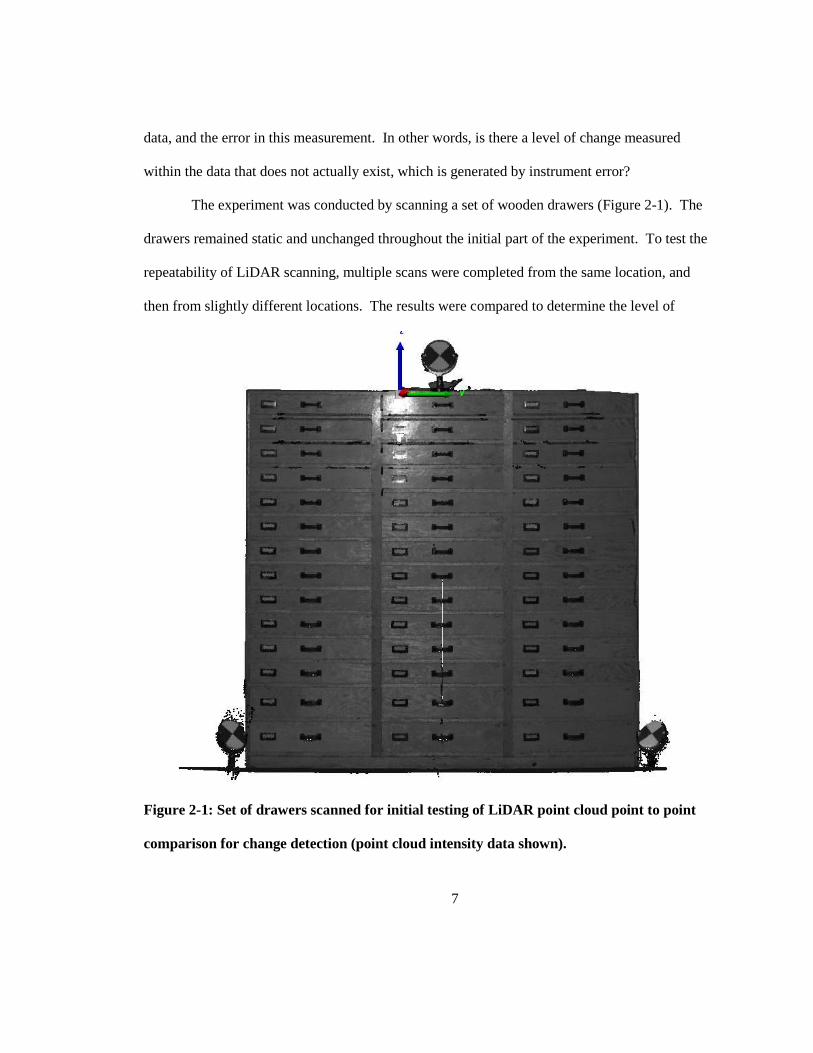
The experiment was conducted by scanning a set of wooden drawers (Figure 2-1). The
drawers remained static and unchanged throughout the initial part of the experiment. To test the
repeatability of LiDAR scanning, multiple scans were completed from the same location, and
then from slightly different locations. The results were compared to determine the level of
Figure 2-1: Set of drawers scanned for initial testing of LiDAR point cloud point to point
comparison for change detection (point cloud intensity data shown).
8
change measured within the data (Figure 2-2). The final step of the experiment was to move one
of the drawers out by a controlled amount and repeat the scan to see if the amount the drawer was
moved correlated well to the amount that was measured by hand.
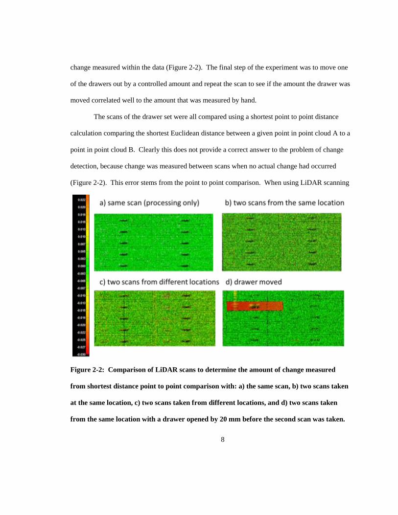
The scans of the drawer set were all compared using a shortest point to point distance
calculation comparing the shortest Euclidean distance between a given point in point cloud A to a
point in point cloud B. Clearly this does not provide a correct answer to the problem of change
detection, because change was measured between scans when no actual change had occurred
(Figure 2-2). This error stems from the point to point comparison. When using LiDAR scanning
Figure 2-2: Comparison of LiDAR scans to determine the amount of change measured
from shortest distance point to point comparison with: a) the same scan, b) two scans taken
at the same location, c) two scans taken from different locations, and d) two scans taken
from the same location with a drawer opened by 20 mm before the second scan was taken.
9
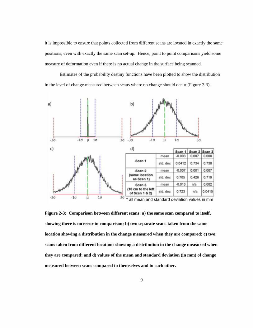
it is impossible to ensure that points collected from different scans are located in exactly the same
positions, even with exactly the same scan set-up. Hence, point to point comparisons yield some
measure of deformation even if there is no actual change in the surface being scanned.
Estimates of the probability destiny functions have been plotted to show the distribution
in the level of change measured between scans where no change should occur (Figure 2-3).
Figure 2-3: Comparison between different scans: a) the same scan compared to itself,
showing there is no error in comparison; b) two separate scans taken from the same
location showing a distribution in the change measured when they are compared; c) two
scans taken from different locations showing a distribution in the change measured when
they are compared; and d) values of the mean and standard deviation (in mm) of change
measured between scans compared to themselves and to each other.
* all mean and standard deviation values in mm
10
To avoid point to point comparison problems and errors, LiDAR data is generally
meshed. The process of meshing creates a surface, and the comparison of two surfaces allows for
the normal or shortest distance between the two surfaces to be compared. This provides a more
accurate comparison of data sets than point to point comparison.
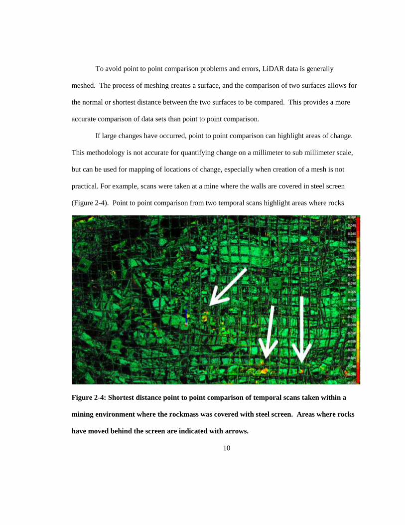
If large changes have occurred, point to point comparison can highlight areas of change.
This methodology is not accurate for quantifying change on a millimeter to sub millimeter scale,
but can be used for mapping of locations of change, especially when creation of a mesh is not
practical. For example, scans were taken at a mine where the walls are covered in steel screen
(Figure 2-4). Point to point comparison from two temporal scans highlight areas where rocks
Figure 2-4: Shortest distance point to point comparison of temporal scans taken within a
mining environment where the rockmass was covered with steel screen. Areas where rocks
have moved behind the screen are indicated with arrows.
11
have moved behind the screen.
It is important to determine the level of change that is going to be measured within the
data sets, and to determine an appropriate method for measuring this deformation. The focus of
this thesis is primarily on the development and testing of the method for measuring convergence,
change and deformation, but initial analysis to determine the level of change expected was
conducted.
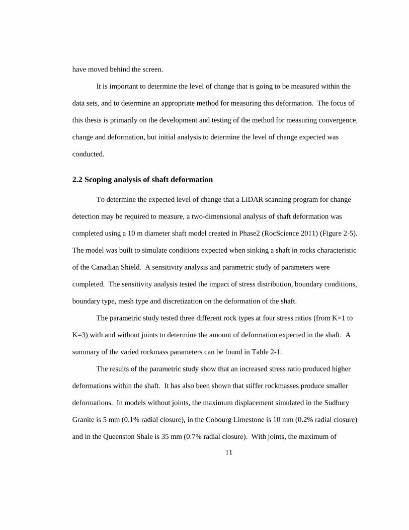
2.2 Scoping analysis of shaft deformation
To determine the expected level of change that a LiDAR scanning program for change
detection may be required to measure, a two-dimensional analysis of shaft deformation was
completed using a 10 m diameter shaft model created in Phase2 (RocScience 2011) (Figure 2-5).
The model was built to simulate conditions expected when sinking a shaft in rocks characteristic
of the Canadian Shield. A sensitivity analysis and parametric study of parameters were
completed. The sensitivity analysis tested the impact of stress distribution, boundary conditions,
boundary type, mesh type and discretization on the deformation of the shaft.
The parametric study tested three different rock types at four stress ratios (from K=1 to
K=3) with and without joints to determine the amount of deformation expected in the shaft. A
summary of the varied rockmass parameters can be found in Table 2-1.
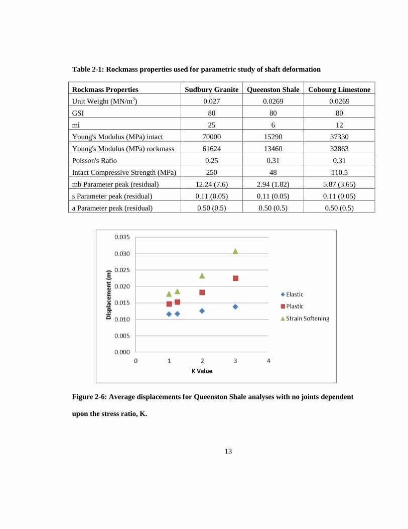
The results of the parametric study show that an increased stress ratio produced higher
deformations within the shaft. It has also been shown that stiffer rockmasses produce smaller
deformations. In models without joints, the maximum displacement simulated in the Sudbury
Granite is 5 mm (0.1% radial closure), in the Cobourg Limestone is 10 mm (0.2% radial closure)
and in the Queenston Shale is 35 mm (0.7% radial closure). With joints, the maximum of
12
Figure 2-5: Example of shaft deformation model created in Phase 2 (RocScience 2011).
Direction of displacement zone and boundary displacement progression (white arrows show
direction of joint failure and deformation zone progression with increased stress ratio,
black arrows show direction of boundary deformation).
displacement simulated in the Sudbury Granite is 7.0 cm (1.4% radial closure), in the Cobourg
Limestone is 10.6 cm (2.1% radial closure), and in the Queenston Shale is 19.6 cm (3.9% radial
closure) (Figure 2-6).
13
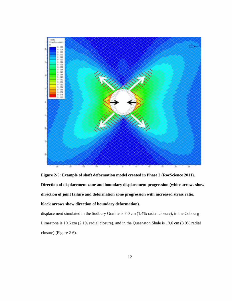
Table 2-1: Rockmass properties used for parametric study of shaft deformation
Rockmass Properties Sudbury Granite Queenston Shale Cobourg Limestone
Unit Weight (MN/m3) 0.027 0.0269 0.0269
GSI 80 80 80
mi 25 6 12
Young's Modulus (MPa) intact 70000 15290 37330
Young's Modulus (MPa) rockmass 61624 13460 32863
Poisson's Ratio 0.25 0.31 0.31
Intact Compressive Strength (MPa) 250 48 110.5
mb Parameter peak (residual) 12.24 (7.6) 2.94 (1.82) 5.87 (3.65)
s Parameter peak (residual) 0.11 (0.05) 0.11 (0.05) 0.11 (0.05)
a Parameter peak (residual) 0.50 (0.5) 0.50 (0.5) 0.50 (0.5)
Figure 2-6: Average displacements for Queenston Shale analyses with no joints dependent
upon the stress ratio, K.
14
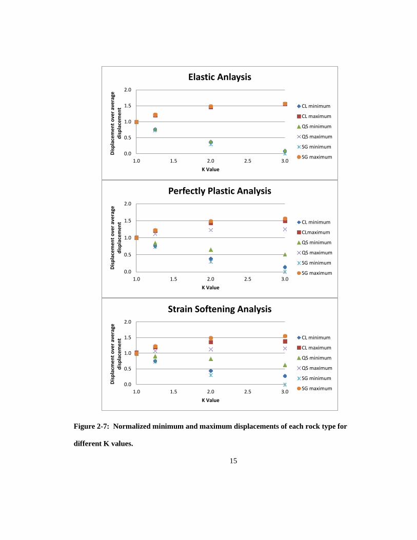
The greatest displacements in the models were always found parallel to the orientation of
maximum stress, while minimum displacements were parallel to the orientation of minimum
stress. In models without joints the zone of greatest displacement is parallel to maximum stress,
whereas in models with joints the zone of greatest deformation extends along the orientation of
the joints (Figure 2-7).
Based on the results of the analysis in some cases of rock deformation it will be important
to measure millimeter scale change over a range of meters, therefore point to point comparison
clearly is not an option. Current surface meshing processing techniques also do not lend
themselves to conveniently analyzing underground convergence measurements and provide no
methodology for quantifying convergence or analyzing different types of deformation.
Therefore, new methods need to be developed that allow for measurement of deformation that is
useful both for convergence analysis and for back calculation of excavation performance.
15
Figure 2-7: Normalized minimum and maximum displacements of each rock type for
different K values.
0.0
0.5
1.0
1.5
2.0
1.0 1.5 2.0 2.5 3.0
Dis
pla
cem
en
t o
ver
ave
rage
d
isp
lace
me
nt
K Value
Elastic Anlaysis
CL minimum
CL maximum
QS minimum
QS maximum
SG minimum
SG maximum
0.0
0.5
1.0
1.5
2.0
1.0 1.5 2.0 2.5 3.0
Dis
pla
cem
en
t o
ver
ave
rage
d
isp
lace
me
nt
K Value
Perfectly Plastic Analysis
CL minimum
CLmaximum
QS minimum
QS maximum
SG minimum
SG maximum
0.0
0.5
1.0
1.5
2.0
1.0 1.5 2.0 2.5 3.0
Dis
pla
cme
nt
ove
r av
era
ge
dis
pla
cem
en
t
K Value
Strain Softening Analysis
CL minimum
CL maximum
QS minimum
QS maximum
SG minimum
SG maximum

16
17
Chapter 3
Development of an Elliptical Fitting Algorithm for Tunnel Deformation
Monitoring with Static Terrestrial LiDAR Scanning1
3.1 Abstract
Terrestrial laser scanning, also known as Light Detection and Ranging (LiDAR) is an
emerging technology that has many proven uses in the geotechnical and geomechanical
engineering community including rockmass characterization, discontinuity measurement and
landslide monitoring. One of the up-and-coming applications of LiDAR scanning is deformation
monitoring and change detection.
Traditionally deformation in tunnels is measured using a series of five or more control
points installed around the diameter of the tunnel and measured at regular time intervals. LiDAR
provides the ability to get a more complete characterization of the tunnel surface, allowing for
determination of the mechanism and magnitude of tunnel deformation, as the entire surface of the
tunnel is being modeled rather than just a fixed set of points. The change in deformation pattern
over time is also much more easily extracted from LiDAR profile analysis.
1 This chapter appears as submitted to an international journal with the following citation:
Delaloye, D., Walton, G., Hutchinson, J., Diederichs, M. (2012) Development of an Elliptical
Fitting Algorithm for Tunnel Deformation Monitoring with Static Terrestrial LiDAR Scanning.
Tunneling and Underground Space Technology.
18
This paper discusses LiDAR scanning for deformation mapping of a surface and for
cross-sectional closure measurements within an active tunnel using elliptical fitting for profile
analysis.
3.2 Introduction
Light Detection and Ranging (LiDAR) is a technology used for quickly acquiring three
dimensional point cloud data. By emitting a laser and measuring either the time elapsed or the
phase shift in the returned beam (depending on the scanner type) the scanner collects both three
dimensional (3D) positional data (x, y, z) and intensity return (i). The newest scanners can collect
up to one million points per second.
Multiple LiDAR scans taken at different times and distances from an advancing tunnel
face can be compared to determine the deformation profile of a tunnel and how it is changing
over time. This information can be useful in back analysis for analyzing stress orientations and
determining the amount and location of support to be installed.
To use a LiDAR point cloud for deformation measurement, appropriate workflows and
data analysis techniques must also be developed. Authors have begun to develop techniques for
deformation monitoring in various geological environments such as tunnels (Van Gosliga et al.
2006), landslides (Jaboyedoff et al. 2009), volcanic environments (Nguyen et al. 2011) and
rockfalls (Abellan et al. 2011). To use LiDAR scan data for tunnel profile analysis and back
calculation, a new method of data analysis involving elliptical fitting has been proposed by the
author. This new method allows for both the best fit ellipses to multiple scans as well as the raw
LiDAR profiles to be analyzed to grain the maximum amount of information from the scan data.
19
3.3 Deformation monitoring in tunnels
During the excavation of a tunnel or other underground space, the in situ stresses are
redistributed around the excavated area. The redistribution of the stress field results in a tendency
for closure of the void created by the excavation. This closure or deformation is generally
referred to as convergence when it occurs in a tunneling environment. The magnitude of
deformation is related to the rockmass conditions, the magnitude, orientation and ratio of the in
situ stresses, the excavation method and rate, and the type and location of installed support.
Monitoring tunnel convergence is an integral part of modern design and construction techniques.
The objectives and requirements of deformation monitoring programs are different for
different tunneling environments. In mountain tunneling environments, small deformations of the
tunnel walls are generally acceptable (centimeters of tunnel closure over meter scale tunnels).
The magnitude of the deformation is monitored to ensure that the temporary support installed
within the tunnel is adequate. Deformations on the scale of centimetres over the tunnel diameter
are allowable in mountain or other remote tunnel environments as the tunnels general have a large
degree of overburden therefore closure of the tunnel has little to no impact at ground surface.
Small tunnel deformations also do not generally influence the final functionality of the tunnel.
Hence in mountainous and remote environments the accuracy of the deformation measurements
can be on the order of a few millimetres.
In contrast, when tunneling in urban environments, even small deformations (on the scale
of millimeters over meter excavations) are generally unacceptable. Any movement will affect
surface infrastructure and the area surrounding the excavation. Therefore in urban environments,
high accuracy, high precision measurements of deformation are necessary. It is of the utmost
20
importance to monitor deformations as close to the face as possible. The goal of monitoring
deformations near the face is to capture as much of the initial deformation (deformation occurring
immediately after excavation) of the profile as possible. Capturing the initial deformation allows
for rapid response and the installation of increased support and modification of excavation
methods if deformations are higher than expected. Traditional monitoring markers cannot be
installed until the excavation has been supported, therefore monitoring can only begin about 2-4
m away from the tunnel face. At this point 60-80% of the deformation has already occurred
(Kavvadas, 2005).
In many tunneling environments, it is important that deformation data is processed in real
time, or near real time. Having real time deformation monitoring data allows for rapid response
to any identified hazards or potential upcoming events indicated by deformations. Although real
time monitoring is extremely beneficial, it is associated with increased expenditure and
necessitates the implementation of more advanced technologies. These drawbacks generally limit
the use of real time monitoring to urban tunneling environments, where the consequences of
excessive deformation are higher than in mountainous or remote tunneling environments.
Monitoring deformations is beneficial when the New Austrian Tunneling Method
(NATM) for tunnel excavation is being used (Wittke et al., 2006). In this method, if deformation
measurements are not consistent with those determined through modelling during initial design,
more support or different excavation methods can be implemented. The magnitude of
deformations recorded can also help refine the final liner design. Furthermore, in squeezing
ground it is difficult at the design stage to predict the magnitude, location and orientation of
convergence, given typical uncertainties in material properties and stress regime. Squeezing
conditions may occur over very short distances (Barla et al., 2008); therefore deformation
21
monitoring is crucial to ensure support is properly installed to maintain the safety and stability of
excavations. In addition, deformations can serve as an early warning for more severe failures.
Results obtained from monitoring programs can also be used to back calculate deformability and
other ground strength data.
3.3.1 Traditional monitoring techniques
There are many existing technologies for measuring tunnel wall convergence. These
include, but are not limited to: tape extensometers, total station surveying (or other geodetic
methods), and laser profilers. Historically deformation in tunnels has been measured using
extensometers or INVAR tapes, which provide the relative displacement between two points
(Kontogianni & Stiros, 2003). With the advent of theodolites and total stations, absolute
distances can be measured and deformations can therefore be linked to external coordinate
systems. Today convergence control points are generally established and measured soon after
excavation and the installation of support. Measurements are then repeated daily until
movements stabilize. In tunneling environments, measurements of deformation are generally
made during construction, and are sometimes continued well after construction is completed if
deformations have not stabilized and continue to pose problems during operation (Kontogianni &
Stiros, 2005).
Tape extensometers are the most accurate of all the commonly used deformation
monitoring technologies (Figure 3-1 a). They have an accuracy of +/- 0.2 mm over 10-15 m
(Kavvadas, 2005). The main drawback with tape extensometers is that they only have the ability
to measure movement along a specific line. They also must be permanently installed in the walls
of the tunnel, which interrupts the construction process of the tunnel. Barla et al. (2008) has
22
demonstrated the technique and utility of measuring convergence by the measurement of
chainages from five control points around a tunnel cross section.
Total station surveying makes use of optical reflectors installed around the tunnel profile
(usually five to seven points) as well as a stable reference point outside the zone of convergence
to measure deformations (Figure 3-1 c). The station must be moved progressively forward from
the location of the stable reference points to the tunnel face, as it progresses. Total stations have
an accuracy of about +/- 2.5 mm over 100 m (Kavvadas, 2005).
Photogrammetric devices require that a number of reference points be installed on the
surface of the tunnel. Photogrammetric devices, where the camera’s position is located using a
total station, have an accuracy of about +/- 5 mm (Kavvadas, 2005).
Some innovative methods for remotely measuring deformation in tunnels include the use
of broken ray videometrics, where a series of relay stations are compared to a reference target
(Qifeng et al., 2008), and the use of charge coupled device (CCD) cameras (digital cameras that
use sensors that convert light to electrical charge instead of film) with targets (Nakai et al., 2005).
The “tunnel convergence monitoring system” developed by Hashimoto et al. (2006) involves the
use of connecting rods, displacement gauges and inclinometers installed at certain cross-sectional
locations. The device places universal displacement gauges in an octagonal shape around the
tunnel profile. The length of the rods and the angle between them is measured, with seven points
to one reference. This method is very accurate, but requires permanent installation of
measurement devices.

23
Figure 3-1: Traditional monitoring of tunnel section using control points. Barla’s technique
defines a) the location of points for chainage array measurements, and b) an example of
displacements of array measurements over time (after Barla 2008). In another plot of tunnel
convergence data (after Schubert et al, 2002), absolute displacement vectors of five control
points are shown in: c) cross section to show vertical movement, and d) longitudinal section
to show lateral translation.

24
3.3.2 Georeferencing and absolute positioning
For the purposes of performance monitoring or back analysis of single or non-interacting
tunnels or shafts, either relative or absolute measurements of tunnel convergence and deformation
can be made. Before the advent of georeferencing, relative measurements were the only option
for measuring tunnel convergence. Today, as total stations and global positioning systems (GPS)
are very common, absolute positioning has become the state of practice for convergence
measurements. The main advantage that absolute positioning provides in tunnel deformation
monitoring is that it adds the ability to measure vertical and lateral shift in the tunnel, as well as
allowing referencing to an external coordinate system (Kontogianni & Stiros, 2003).
Although it is often assumed that absolute positioning is necessary to characterize
deformation, this is not the case. Data examined using relative convergence techniques provides
the same quality of stability information and back analysis capability as using absolute
positioning measurements. In a single bore tunnel, where diametric convergence is being
measured, there is no direct benefit to implementing absolute positioning. Absolute positioning is
necessary in twin bore tunnels, however, when the vertical and lateral shift in one tunnel can
affect the stability of the other tunnel. Absolute positioning and displacement measurement may
also be required where surface settlement or building interaction is being monitored.
When using relative positioning to characterize tunnel convergence it is important to
consider the diametric convergence instead of the radial convergence, to ensure any errors due to
the misalignment of the centroid of the tunnel are eliminated (Figure 3-2).
25
Figure 3-2: a) The tunnel profile shown has been translated but has experienced no
convergence. b) The measured radial convergence between the tunnel profiles shown in a)
based on radial measurement from the centroid of the first shape. c) The measured relative
diametric convergence between the tunnel profiles shown in a).
3.3.3 Permanent referencing in an active tunneling environment
To implement any type of deformation monitoring near the face in a tunneling
environment where a tunnel boring machine (TBM) is being used, absolute positioning is likely
not possible. Data will need to be collected rapidly, and possibly with little warning or time for
preparation, when a break in the TBM operations permit access for scanning the tunnel. The
locations for measurement must also be flexible. Occlusion of areas of the tunnel wall will be
inevitable as parts of the tunnel wall will be blocked by machinery, ventilation, conveyor systems
or the TBM itself.
Furthermore, in an active tunnelling environment, it is not always practical or possible to
maintain permanent survey markers. For total station measurements of convergence, prisms are
usually installed at certain sections around the perimeter of the tunnel. If one of these prisms is
26
knocked out of place or comes loose, convergence measurements can no longer be made from
that point. Also, if one of the prisms were installed in an area of anomalous movement, the data
collected would be useful for characterizing that section of deformation, but would not provide
information that could be used for back analysis.
3.3.4 Back analysis using deformation measurements
One of the main reasons deformation measurements are collected is for back analysis.
Back analysis is useful for monitoring the stability of excavations, for calculation and
interpretation of field stresses, and for calculation of rockmass parameters such as deformability.
Many authors have explored different methods for using monitoring results for back analysis in
tunnels and other underground excavations (Chan & Stone, 2005, Vardakos et al., 2006, Sakuri &
Takeuchi, 1983, Russo et al., 2009, Oreste, 2004, Zhifa et al., 2004). The development of a
complete methodology for back calculation of rockmass parameters and back analysis of stress
orientations from LiDAR data is beyond the scope of this paper, but LiDAR data can be of added
benefit to existing techniques.
3.4 Accuracy and noise in LiDAR scanning
Before LiDAR data is collected, the necessary accuracy and resolution of that data to be
collected must be determined. The end use of the data is the main factor that contributes to the
maximum allowable accuracy and minimum allowable resolution. In general, the level of error in
a data set must be less than the resolution of the object or quantity being measured. To minimize
error in LiDAR data it is important to be familiar with the sources of error associated with data
acquisition. These can be broken into:

27
the error in the range measurement
the error in the vertical angle measurement
the error in the horizontal angle measurement
The error in range measurement increases with distance from the scanner. The main
components are the spot size of the laser, the reflectivity of the object being scanned, and the
angle of incidence between the scanner and the object. Error in range measurement is minimized
by choosing appropriate scan locations and settings.
Angular error, broken into the error in the vertical and horizontal angle measurement, is
associated with the scanner’s measurement of one or more of its moving parts, and therefore can
be minimized by using a properly calibrated scanner.
Other errors within LiDAR data sets can be introduced during field procedures for
scanning and processing of the LiDAR point cloud data such as errors in positioning
measurement in the field and poor alignment of scans during processing. Erroneous points, also
referred to as spurious scan points (Jacobs, 2009), are additional sources of error in LiDAR
scanning and are often associated with poor atmospheric conditions, interfering radiation, or
highly reflective surfaces such as spectral reflectors.
3.4.1 Non scan related noise
There are other sources of “noise” that impact LiDAR scanning in an underground
environment that are not associated with the scanning itself. “Noise” here is defined by the
author to be anything that creates deviation from a perfectly circular tunnel design profile. These
sources of noise include:
Roughness of the rock surface
28
Systematic undulation of the profile (caused by excavation type)
Noise created by structure within the rockmass
Anomalies on the tunnel surface (e.g. rockbolts, faceplates, screen)
Occlusion of the profile by obstructions
3.5 Terrestrial LiDAR scanning for deformation monitoring in tunnels and shafts
As LiDAR scanning is becoming a more common surveying device, new applications for
LiDAR scanning are arising. The most recent and promising application of LiDAR scanning is
for deformation monitoring. Experiments have been conducted to determine if the error within
LiDAR data is small enough to measure millimetric deformations (Abellan et al., 2009). In
general, the level of error within survey data must be less than the minimum level of change of
the physical quantity measured (Simeoni & Zanei, 2009). Due to the large number of high
accuracy, high precision data points collected during LiDAR scanning it is possible to use
statistical techniques to measure levels of change within the level of precision of the LiDAR scan
data. What this means is that even if the LiDAR point cloud only has millimeter precision,
millimeter scale change can be measured using statistical analysis of the data. A review of
previously completed work demonstrating the use of LiDAR scanning for geological applications
and for deformation monitoring is discussed in the following sections.
3.5.1 Applications of LiDAR scanning in Geological Engineering
Many authors have demonstrated the use of LiDAR scanning for geological engineering
applications, the most common use being the extraction of rockmass discontinuity data (Fekete et
al. 2010, Gigli & Casagli, 2011, Lato et al., 2009, Otto et al., 2011, Poropat, 2006, Slob, 2010,
29
Slob et al., 2007, Sturzenegger & Stead, 2009). LiDAR has also been used for large-scale
roughness calculation using the roughness length measurement technique (Rahman et al, 2006,
Tesfamariam, 2007) and recently, LiDAR scan data has been used for discrimination between
lithological units in sedimentary rocks (Burton et al., 2010). The main applications of LiDAR
scanning in tunnels and shafts to date has been for as-built modeling, rockmass characterization
(Fekete et al., 2010), and for quality control and assurance, such as the calculation of shotcrete
thickness and rockbolt spacing. Fekete et al. (2010, 2012) have also used LiDAR data to locate
areas of seepage in the rockmass, map structures in the face of the tunnel, structurally map and
document sections of overbreak, and to extract joint models for implementation into discrete
element models.
Seo et al. (2008) used tunnel cross section analysis to measure overbreak and underbreak,
and showed the economic viability of this measurement. The extracted cross-sections were
analyzed in CAD and compared to design sections. Volume of overbreak was calculated using a
range in the number of data points, but the method for cross sectional volume calculation was not
demonstrated.
The use of LiDAR in a tunneling environment has also been shown by Decker & Dove
(2008) in the Devil’s Slide tunnels in California. Here, LiDAR was used to compare excavation
profiles against design profiles for quality control of shotcrete thickness, profile and smoothness,
for geological documentation, and for rockmass classification.
3.5.2 Deformation monitoring with LiDAR
Deformation monitoring using terrestrial laser scanning is gaining attention due to the
high point density and spatial resolution that can be acquired in a minimal amount of time, but the
30
use of laser scanning for deformation monitoring is still in its infancy. Authors have begun to
develop techniques for using LiDAR scanning for deformation monitoring of various objects,
such as a television tower (Schneider, 2006), an old cooling tower (Ioannidis et al., 2006),
concrete and wooden beams (Gordon & Lichti, 2007) and in geological environments such as
landslide areas (Hui et al., 2010, Jaboyedoff et al., 2009, Monseratt & Crosetto, 2008, Oppikofer
et al., 2009, Slob & Hack, 2004,), volcanic environments (Nguyen et al., 2011) and rockfalls
zones (Abellan et al., 2011, Scaioni & Alba, 2010).
Schneider (2006) demonstrated the use of terrestrial laser scanning for deformation
monitoring of a television tower by taking sections of the tower in the z plane, the plane defined
by a normal parallel to the tower axis, and calculating the area of the sections to determine the
amount of bending in the tower.
Monseratt & Crosetto (2008) estimated deformation of landslides using terrestrial laser
scanning data processed using local surface matching techniques. The methodology involves co-
registration of point clouds, using a least squares fitting algorithm, for areas that are assumed to
be stable. After the surfaces from two different time periods are matched, the displacement
vectors are extracted. An assumption is made that the slide is a rotational failure with a simple
circular slip surface.
Slob & Hack (2004) demonstrated the use of time of flight scanning for calculating
volume change in earth fill and soil heaps. They showed about 5 to 10 mm resolution in the
measurements of deformation. Although the measurement of deformation of a landslide is a
similar problem to scanning within tunnels, measuring the change in a soil heap is actually a 2.5D
problem, not a truly 3D problem as the change in volume can be measured relative to the z plane,
which here is the horizontal plane. In a tunnel, change must be measured relative to the centroid
31
of the tunnel therefore the change cannot be compared using a projection onto the z plane as in
the case of a landslide.
Tsakiri et al. (2006) has suggested that deformations smaller than the magnitude of
single-point precision of the scanner can be measured by deriving best-fitting surface models. To
make use of best-fitting surfaces, pre-processing to eliminate noisy and erroneous data must be
completed. The method proposed by Tsakiri et al. (2006) has been applied to planar surfaces
successfully, but has not been extended to rough, undulating, or curved surfaces as would be
found in underground excavations.
3.5.3 Previous work in LiDAR scanning for monitoring tunnel deformation
Completing full surface deformation characterization in tunnels is beneficial as it can
allow for greater understanding into the mechanism through which rockmasses react to
excavation, and allow for the prediction of potential stability issues (Lemy et al., 2006). As such,
the next logical application of LiDAR in underground environments is for the measurement of
deformation. Authors have begun to demonstrate methods for applying LiDAR scanning to
tunnel deformation monitoring (Van Gosliga et al., 2006, Lemy et al., 2006, Lindenberg et al.,
2005, Lindenberg et al., 2009, Nuttens et al., 2010).
Van Gosliga et al. (2006) are one of the first in the literature to demonstrate a
methodology for measuring deformation in tunnels using terrestrial laser scanning. Van Gosliga
et al. (2006) decimated the LiDAR scan to deal with only 1% of the data, reducing the point cloud
data to a 15 cm by 15 cm grid. Scanning was completed in a concrete segment lined tunnel,
where roughness of the surface was of minimal concern. Their methodology used raster
partitioning over a cylinder to compare scans of different epochs using a computational program
32
written in Matlab. The scan data is partitioned into cells and the raster is laid out over the object.
During the experiment scans were taken hours apart with objects added to the surface of the
tunnel to simulate deformation. The scan data was fit to the cylinder using a least squares
adjustment.
Van Gosliga et al. (2006) indicated that it remained to be determined if the amount of
deformation measured was real or due to measurement noise, and did not test whether using a
higher percentage of the original data set changed the results of the measurement of deformation
in a meaningful way. Furthermore, they suggested that the results of deformation analysis using
terrestrial laser scanning would be improved when the behavior of scan accuracy was better
understood.
Lemy et al. (2006) proposed a method for monitoring deformation in LiDAR scans by
matching scan points to total station survey markers. Similar to Van Gosliga et al. (2006), Lemy
et al. (2006) characterized deformation by fitting a surface to the LiDAR data and interpolating
the scan points over a localized grid.
A methodology for measuring deformation with LiDAR in rectangular tunnels was
created by Lindenberg et al. (2009). A simple region grown from a seeded point, similar to
region grows used for joint extraction (Slob et al., 2007), was used to define segments of data. A
data point is chosen and the normal vector of the point is estimated based on fitting a plane to its
nearest neighbors. If the points defining the plane result in a large root mean square error
(RMSE) the point is discarded as a single point, and another data point is chosen to start the
process. The region grow continues until the threshold for the RMSE is reached. The data was
segmented by Lindenberg et al. (2009) to allow for selection of near planar regions of points that
were then fit with a best fit plane, and the deviation of the points from the plane were calculated.
33
Nuttens et al. (2010) has also demonstrated a method for determining deformation within
a concrete segment lined tunnel using LiDAR data. A triangular irregular network (TIN) was
created from the LiDAR data and then a cross section of the tunnel was extracted from the TIN.
The locations of sequential cross sections based on different scans of the tunnel were taken
through reference targets installed on the tunnel walls to ensure that the sections were extracted
from the same locations. The main limitation of this approach is that a TIN is not truly three
dimensional, therefore is not a completely accurate representation of the tunnel profile. During
the creation of a TIN, a surface is created by projecting from a single direction. No two points
can exist with a third coordinate equal in this direction. For example, if a TIN were created by
projecting onto a surface in the x,y direction, no two points could have the same z coordinate,
hence a TIN is not truly 3D.
Nuttens et al. (2010) also used a 51 point moving average calculation to smooth the
surface of the TIN, which had little impact on the accuracy of the analysis due to the smoothness
of concrete segments, but would have a large impact on results for deformation in an unlined
tunnel.
To date, no systematic methodology for using LiDAR in an active or unlined tunneling
environment to measure deformation has been created.
3.5.4 Benefits of LiDAR scanning for deformation monitoring
As previously mentioned, the high point density and spatial resolution of LiDAR data
allows for full surface characterization. There are additional benefits to using LiDAR scanning
for deformation measurement including its ability to be implemented without interruption of the
construction sequence, and the lack of necessity for permanent referencing. Furthermore, it is not

34
important to carefully select sections for subsequent deformation analysis, prior to monitoring, as
any location within the tunnel can be extracted from the LiDAR scan for analysis, as long as
scans are taken at spacing close enough to provide full coverage.
The ability of LiDAR scanning to be implemented into tunnel construction, without
interruption of the excavation sequence, has been shown by Fekete et al. (2010). Although
Fekete et al. (2010) were not using the scanned data to determine deformation, little change in the
scanning protocol they developed is necessary to permit deformation detection from temporal
scans.
As shown in this thesis, with LiDAR, it is possible to measure deformation and
convergence without using a total station to locate the device and without installation of any
permanent reference markers.
As LiDAR scanning offers less raw single point precision than traditional tunnel
convergence monitoring techniques (Lindenberg et al., 2005), it is best suited for broader surface
analysis rather than for measurement of specific points of movement, particularly because it is
impossible to exactly locate and scan the same point in subsequent LiDAR scans. Hence, LiDAR
must use either full surface analysis or statistical techniques for measurements of change.
3.5.5 Limitations and errors in current analysis techniques
When dealing with LiDAR data for quantitative analysis or, specifically, change
detection, it is not sufficient to look at raw point cloud data. Post processing is necessary to
generate usable data. Only in recent years have computing and software developments become
robust enough to allow users to handle and process massive data sets. Buckley et al. (2008)
provided a typical workflow used for collecting and processing LiDAR data for geological
35
applications. Although they defined a workflow specifically for outcrop mapping, many of the
same steps can be used for underground LiDAR mapping.
LiDAR scanning it is best suited for surface analysis, rather than specific point analysis.
It should also be noted that it is generally not possible to exactly locate and scan the same
individual surface point in a LiDAR scan.
General purpose algorithms are often not sufficient for specific purposes such as change
detection. It is not appropriate, for example, to use the built-in PolyWorks® V 11.0.28
(InnovMetric, 2011) calculation of shortest distance as, in this case, shortest distance is normally
an underestimation of the total displacement or change. It is more appropriate to use the normal
distance from a specified reference surface (tunnel cylinder or arc), comparing the distance to the
old surface (original profile) with the distance to the new surface (deformed profile).
In standard LiDAR data processing using software like PolyWorks® V 11.0.28
(InnovMetric, 2011), the data is interpolated twice before any measurements are extracted. The
data is initially interpolated when loaded into the program to allow each interpolated point to be
assigned a normal direction based on its relation to its nearest neighbors. A second interpolation
occurs when the data is meshed. Every interpolation introduces a small amount of error into the
data, and means that the user is one step further away from working with the initial collected data
set.
Another drawback of current deformation monitoring techniques using LiDAR scanning
is the necessity for meshing the LiDAR data. Not only is this a second interpolation of the data,
which in itself adds a level of error to the data, but also meshing itself can create erroneous
surfaces. A clear example of this is shown when a scan of a tunnel shaft where the walls have
been covered in screen. It is impractical to try and pre-process the data to eliminate the screen
36
within a scan, as it is almost impossible to discern between the screen and the tunnel wall behind.
Currently no filtering algorithms exist for removing one surface layer (screen) from another (rock
surface) in LiDAR data sets. If the data is meshed without removing the screen, the screen and
the bare rock are meshed as one surface. This is clearly an erroneous surface, and cannot be used
for any type of deformation or profile analysis.
Another limitation of current software based deformation mapping techniques is that it is
limited to color display of shortest distances. As previously mentioned, using shortest distance
calculation between profiles leads to an underestimation in the amount of deformation of the
tunnel. The color display is a useful visualization technique but it is more beneficial to actually
extract quantitative deformation profile data. The Matlab code written as part of this thesis
automatically produces deformation profile graphs.
The current programs do allow for a volume change calculation, but this is a
unidirectional volume change calculation and must be taken in reference to a given plane. This
methodology works well, for example, when shotcrete volume needs to be calculated for an area
sprayed on the roof of the tunnel. It is not beneficial though for calculating the volume change of
a tunnel that is squeezing in every direction.
3.6 Ellipse fitting for tunnel deformation analysis
Tunnel convergence measurements are usually analyzed by plotting each point or
chainage measurement separately. Terzaghi (1942) introduced a method to instead fit an ellipse
to the displaced points and determine the mean deformation ellipse. The mean deformation
ellipse allows for different periods of deformation to be more easily characterized than by looking
at single measurements of displacement. For example, one can clearly discern periods of vertical
37
compression from those of horizontal compression. Terzaghi’s (1942) ellipse fitting method
allows for the identification of patterns within convergence measurements more easily than by
looking at convergence measurements alone (Stiros & Kontogianni, 2009).
Historically, use of the Terzaghi’s (1942) mean deformation ellipse has been limited due
to a limited number of profile measurements. With the advent of LiDAR and other fast point
acquisition technologies, this method is becoming more feasible.
To use an ellipse for convergence measurement, it is generally assumed, for the purpose
of back calculation, that plane strain conditions exist, which is valid as this assumption is
common practice at distances greater than two diameters from the tunnel face. The use of the
deformation ellipse also assumes an initially circular section that deforms gradually over time.
One of the main benefits of using an ellipse to define deformations is that the change in the
elliptical profile over time defines a two dimensional tensor that can be used to characterize
deformation.
The long and short axes of the ellipse correspond to the principal deformation directions
within the tunnel. To calculate the amount of normalized tunnel convergence, uniform
deformation between measurements must be assumed. The orientation of the ellipse can easily be
calculated, and is important to identify because a change in the orientation of the ellipse suggests
a change in the deformation pattern. In other words, the directions of minimum and maximum
deformation have changed over time.
Changes in deformation pattern are not easy to discern from convergence measurements
when they are analyzed alone. The shape and the orientation of the ellipse, along with back
analysis of these parameters allow for information on the mechanisms of deformation to be
gained, which can be applied to future decision making for a given tunneling project.
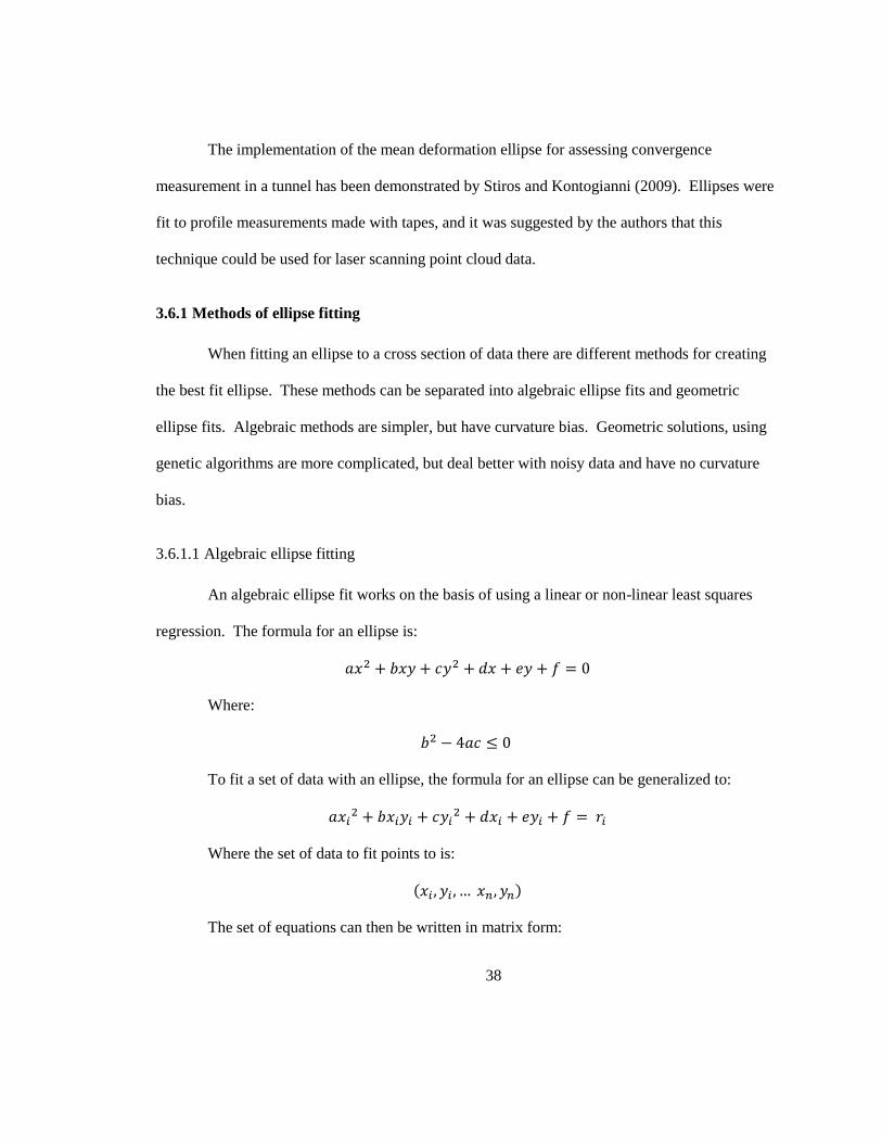
38
The implementation of the mean deformation ellipse for assessing convergence
measurement in a tunnel has been demonstrated by Stiros and Kontogianni (2009). Ellipses were
fit to profile measurements made with tapes, and it was suggested by the authors that this
technique could be used for laser scanning point cloud data.
3.6.1 Methods of ellipse fitting
When fitting an ellipse to a cross section of data there are different methods for creating
the best fit ellipse. These methods can be separated into algebraic ellipse fits and geometric
ellipse fits. Algebraic methods are simpler, but have curvature bias. Geometric solutions, using
genetic algorithms are more complicated, but deal better with noisy data and have no curvature
bias.
3.6.1.1 Algebraic ellipse fitting
An algebraic ellipse fit works on the basis of using a linear or non-linear least squares
regression. The formula for an ellipse is:
Where:
To fit a set of data with an ellipse, the formula for an ellipse can be generalized to:
Where the set of data to fit points to is:
( )
The set of equations can then be written in matrix form:
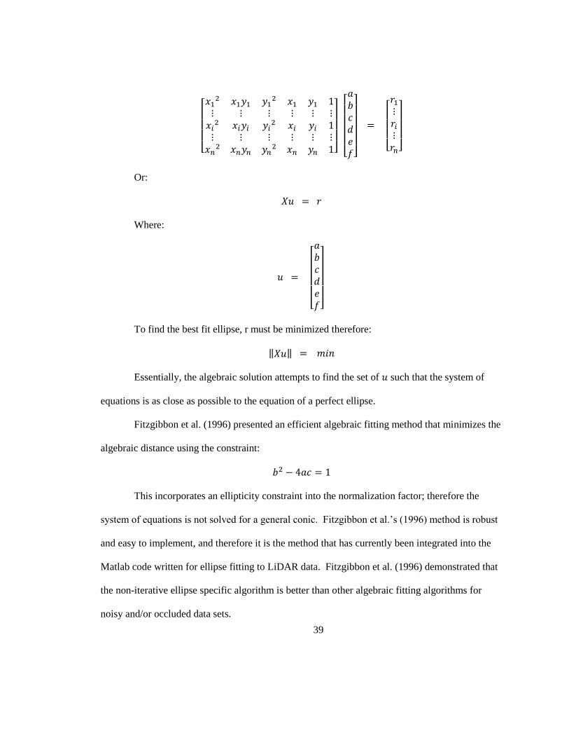
39
[
]
[ ]
[ ]
Or:
Where:
[ ]
To find the best fit ellipse, r must be minimized therefore:
‖ ‖
Essentially, the algebraic solution attempts to find the set of such that the system of
equations is as close as possible to the equation of a perfect ellipse.
Fitzgibbon et al. (1996) presented an efficient algebraic fitting method that minimizes the
algebraic distance using the constraint:
This incorporates an ellipticity constraint into the normalization factor; therefore the
system of equations is not solved for a general conic. Fitzgibbon et al.’s (1996) method is robust
and easy to implement, and therefore it is the method that has currently been integrated into the
Matlab code written for ellipse fitting to LiDAR data. Fitzgibbon et al. (1996) demonstrated that
the non-iterative ellipse specific algorithm is better than other algebraic fitting algorithms for
noisy and/or occluded data sets.

40
3.6.1.2 Geometric ellipse fitting
Genetic algorithms are useful for solving complicated multi-variable non-linear inverse
problems. To complete a geometric ellipse fit, the goal is to minimize the Euclidean distance
from any point to the corresponding point on an ellipse (Figure 3-3).
The parametric equation for an ellipse is:
[ ] [
] [
] [ ]
Where:
( ) is the centre of the ellipse
is the length of the longest axis
is the angle of inclination of the axis of length from the axis
is the length of the axis that is perpendicular to
is the parameter that runs from 0 to 2π anti-clockwise from the major
axis (to point)
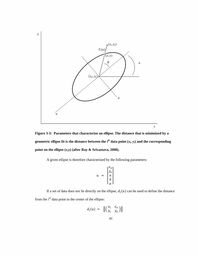
41
Figure 3-3: Parameters that characterize an ellipse. The distance that is minimized by a
geometric ellipse fit is the distance between the ith
data point (xi, yi) and the corresponding
point on the ellipse (x,y) (after Ray & Srivastava, 2008).
A given ellipse is therefore characterized by the following parameters:
[ ]
If a set of data does not lie directly on the ellipse, ( ) can be used to define the distance
from the ith data point to the center of the ellipse:
( ) ‖(
)‖

42
The distance from the center of the ellipse along the same line that connects the center to
( ) to a point on the ellipse is:
( ) ‖ [
] [
]‖
√( )
Thus we can define the distance from the ith data point to the point on the ellipse as:
( ) ‖ ( ) ( )‖
The goal of the ellipse fitting algorithm is to minimize ( )
This involves solving the non-linear least squares problem. To minimize ( ), the
model needs to be found such that:
( ) ∑ ( )
To solve this equation φ must be known. With ( ) the angle of from is
calculated using the point on the ellipse ( ) and the centre of the ellipse ( )
The slope of the line ( ) that connects ( ) and ( ) is:
As are known and are known it is easy to calculate .
To use the genetic algorithm for solving complicated multi-variable non-linear inverse
problems, some initial conditions and estimations must be made. For ellipse fitting it is clear that
( ) must lie within the area defined by the point cloud. The length of the long axis also
cannot exceed the diagonal of the most extreme ( ) coordinates. can be restricted to (0,
)
as either the short axis or the long axis must lie in the first quadrant.
43
Ray & Srivastava (2008) have demonstrated that the geometric solution is more robust
for ellipse fitting to noisy data, where only partial data sets are acquired. Although genetic
algorithms are very powerful, and the geometric ellipse fitting algorithm has proven to produce
better results than algebraic fitting algorithms, it is not considered useful at this point for
processing LiDAR data. The genetic algorithm is computationally much more intensive and is
preferable when only a few data points exist. Genetic algorithms are of a greater advantage when
the number of points acquired is low, and the noise in the points is high. However this approach
has not been considered to be the best option for fitting to LiDAR profile data due to the large
number of data points available from a single scan. It is suggested however, that testing of
genetic algorithm fits on LiDAR data be performed to test this hypothesis in the future.
3.7 Tunnel profile analysis with LiDAR
To analyze tunnel convergence it is appropriate to look at multiple cross sections
throughout the tunnel. To complete cross section analysis of LiDAR data, a new methodology
has been developed in Matlab. Prior to cross section extraction, the following steps must be
taken:
Collect LiDAR scan data in the field
Upload scan data
Trim scans to the area of interest
Clean and filter data
Align multiple scans of same area
Create surface or mesh from point cloud data
Extract cross sections
44
The data must be cleaned to remove all erroneous and spurious scan points. Objects
within the scan that are not part of the tunnel profile, such as machinery or people must also be
removed. If there is screen or other support installed on the surface of the tunnel walls this does
not have to be removed during pre-processing. A filter has been built into the Matlab code, as
part of this thesis, that will serve to remove screen or other physical objects on the tunnel surface
that are not easily filtered out in pre-processing.
After the initial cleaning of the LiDAR data, the scan of the tunnel must be aligned such
that the z axis is the up direction, and the tunnel axis is aligned parallel to either the x or y axis.
Alignment in such a manner allows for cross sections to be accurately extracted along the plane
perpendicular to the heading direction of the tunnel. This coordinate orientation is also necessary
for the cross section to be compatible with the Matlab code.
When comparing multiple scans it is important to extract a cross section from the same
location within the tunnel. It is therefore desirable, but not necessary, to use a best fit algorithm
to align the two point clouds. This ensures that as close as possible to the same cross section is
extracted from both scans. The Iterative Closest Point (ICP) algorithm for alignment of point
clouds is a data driven registration method first proposed by Besl & McKay (1992). This is a
widely used algorithm, and is the built in registration method for most software programs,
including PolyWorks® V 11.0.28 (InnovMetric, 2011). The goal of the ICP is to create the best
alignment between the data shape ( ) and the model shape ( ). In the case of LiDAR point
cloud alignment, the first point cloud for alignment ( ) will be used in place of the model
shape, and the second point cloud ( ) will be used in place of the data shape. The distance ( )
45
between an individual point ( ) in the first point cloud and its closest point in is minimized
by the algorithm:
( ) ‖ ‖
Each point in and its closest point in form a correspondence. The ICP algorithm
completes a least squares regression to minimize the sum of the mean square distance errors
between the correspondences. A detailed description of the algorithm used to complete the
transformation is beyond the scope of this paper but can be found in Besl & McKay (1992).
Alignment of scans from multiple different time periods allows for easier extraction of
the same cross section for comparison. As no absolute positioning is incorporated in this method
of LiDAR deformation analysis, the best way to align scans is by ICP algorithm. The algorithm
used by the author is built in to PolyWorks® V 11.0.28 (InnovMetric, 2011). To complete an
alignment, a large look window is initially used for rough alignment (i.e. 1 m). This window is
progressively decreased until it reaches a level equal to the calculated noise level within the data.
By progressively decreasing the look window to the level of data noise, non-deformed areas
should automatically be the only areas used by the end of the alignment. It is still important for
the user to check the data to ensure a logical alignment of the data has been made and to select the
areas of cross section extraction with care.
There are two proposed methods of cross section extraction. Either a mesh can be
created from the LiDAR scan data, and a cross section extracted from the new surface, or a
narrow swath of point cloud data can be used. Both of these methods allow for elimination of
errors associated with an attempt at direct point to point comparison, and reduction of errors
associated with noise in the data.
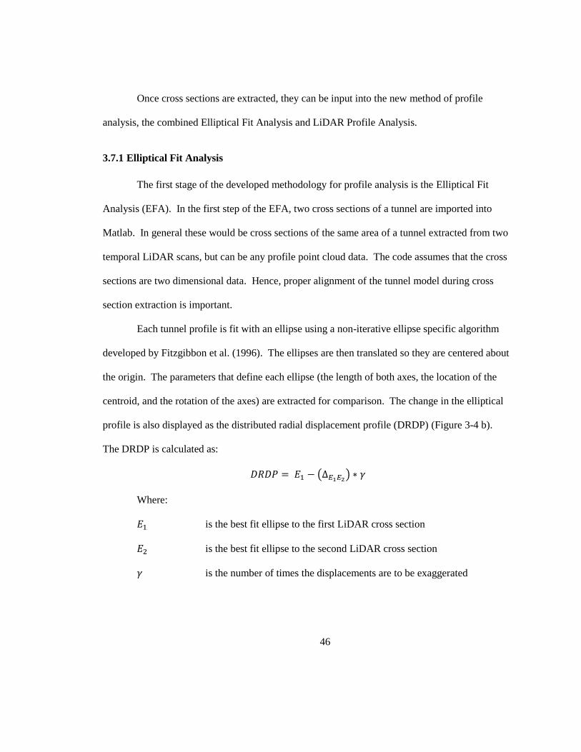
46
Once cross sections are extracted, they can be input into the new method of profile
analysis, the combined Elliptical Fit Analysis and LiDAR Profile Analysis.
3.7.1 Elliptical Fit Analysis
The first stage of the developed methodology for profile analysis is the Elliptical Fit
Analysis (EFA). In the first step of the EFA, two cross sections of a tunnel are imported into
Matlab. In general these would be cross sections of the same area of a tunnel extracted from two
temporal LiDAR scans, but can be any profile point cloud data. The code assumes that the cross
sections are two dimensional data. Hence, proper alignment of the tunnel model during cross
section extraction is important.
Each tunnel profile is fit with an ellipse using a non-iterative ellipse specific algorithm
developed by Fitzgibbon et al. (1996). The ellipses are then translated so they are centered about
the origin. The parameters that define each ellipse (the length of both axes, the location of the
centroid, and the rotation of the axes) are extracted for comparison. The change in the elliptical
profile is also displayed as the distributed radial displacement profile (DRDP) (Figure 3-4 b).
The DRDP is calculated as:
( )
Where:
is the best fit ellipse to the first LiDAR cross section
is the best fit ellipse to the second LiDAR cross section
is the number of times the displacements are to be exaggerated
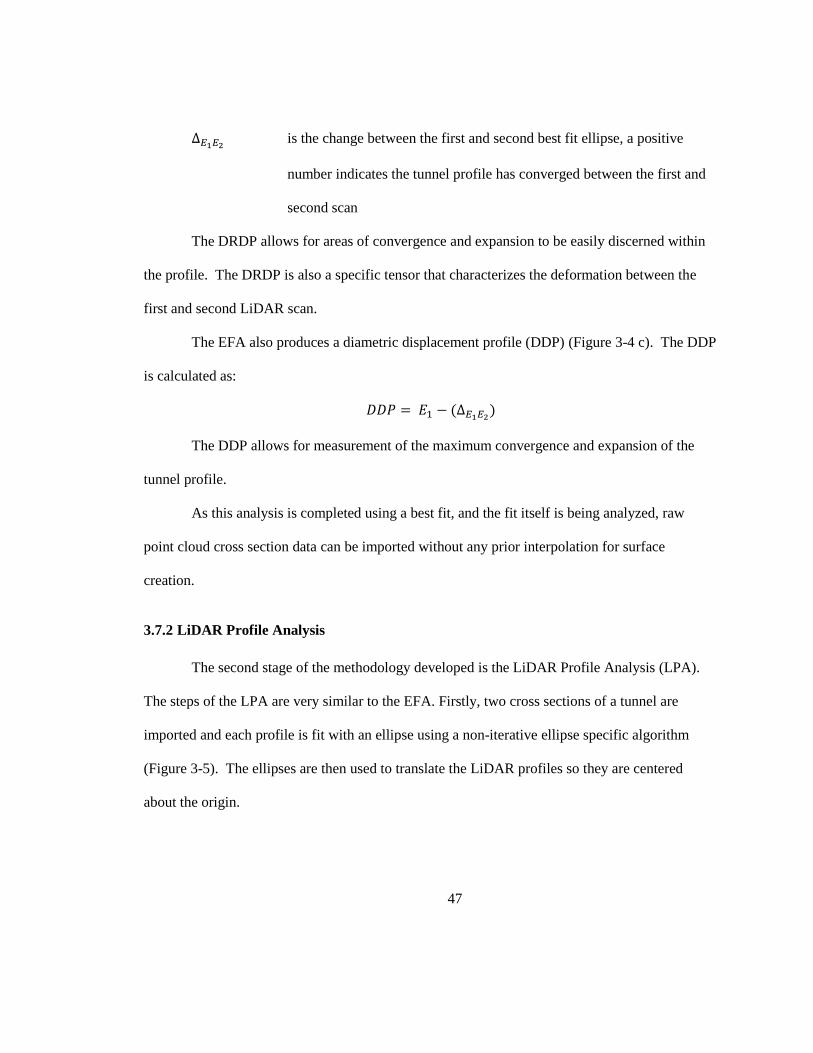
47
is the change between the first and second best fit ellipse, a positive
number indicates the tunnel profile has converged between the first and
second scan
The DRDP allows for areas of convergence and expansion to be easily discerned within
the profile. The DRDP is also a specific tensor that characterizes the deformation between the
first and second LiDAR scan.
The EFA also produces a diametric displacement profile (DDP) (Figure 3-4 c). The DDP
is calculated as:
( )
The DDP allows for measurement of the maximum convergence and expansion of the
tunnel profile.
As this analysis is completed using a best fit, and the fit itself is being analyzed, raw
point cloud cross section data can be imported without any prior interpolation for surface
creation.
3.7.2 LiDAR Profile Analysis
The second stage of the methodology developed is the LiDAR Profile Analysis (LPA).
The steps of the LPA are very similar to the EFA. Firstly, two cross sections of a tunnel are
imported and each profile is fit with an ellipse using a non-iterative ellipse specific algorithm
(Figure 3-5). The ellipses are then used to translate the LiDAR profiles so they are centered
about the origin.
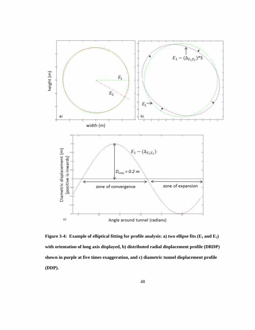
48
Figure 3-4: Example of elliptical fitting for profile analysis: a) two ellipse fits (E1 and E2)
with orientation of long axis displayed, b) distributed radial displacement profile (DRDP)
shown in purple at five times exaggeration, and c) diametric tunnel displacement profile
(DDP).
49
LPA uses the LiDAR point data instead of the elliptical fit to the data. The change in the
LiDAR profile is used to calculate the DRDP and the DDP, exchanging and for and
, where:
is the first LiDAR cross section
is the second LiDAR cross section
Therefore the DRDP (Figure 3-5 b) becomes:
( )
And the DDP (Figure 3-5 c) is calculated as:
( )
For the LPA analysis, and are extracted from surface models of the LiDAR data,
so and are not raw points. By definition the comparison of and is a surface to
surface or mesh to mesh comparison.
Additionally, the LPA calculates the areas of volume increase and volume decrease from
the LiDAR tunnel profiles (Figure 3-6). Instead of a unidirectional comparison, the volumes are
calculated with respect to the center of the tunnel, therefore a more accurate volume is found than
if a unidirectional shortest distance comparison were completed.
To characterize the noise of the LiDAR scan data, the LPA analysis also includes the
generation of a noise profile (NP). The noise profile is the calculated deviation between the
LiDAR profile and the elliptical fit to that LiDAR data (Figure 3-7):
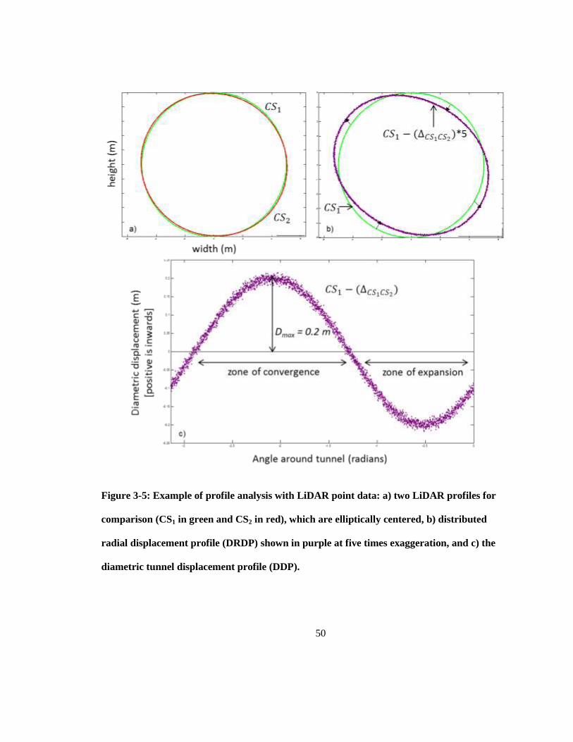
50
Figure 3-5: Example of profile analysis with LiDAR point data: a) two LiDAR profiles for
comparison (CS1 in green and CS2 in red), which are elliptically centered, b) distributed
radial displacement profile (DRDP) shown in purple at five times exaggeration, and c) the
diametric tunnel displacement profile (DDP).
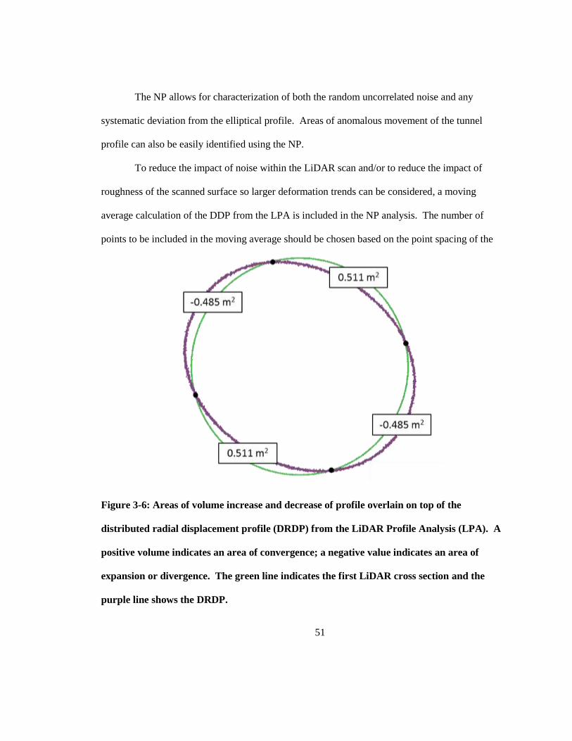
51
The NP allows for characterization of both the random uncorrelated noise and any
systematic deviation from the elliptical profile. Areas of anomalous movement of the tunnel
profile can also be easily identified using the NP.
To reduce the impact of noise within the LiDAR scan and/or to reduce the impact of
roughness of the scanned surface so larger deformation trends can be considered, a moving
average calculation of the DDP from the LPA is included in the NP analysis. The number of
points to be included in the moving average should be chosen based on the point spacing of the
Figure 3-6: Areas of volume increase and decrease of profile overlain on top of the
distributed radial displacement profile (DRDP) from the LiDAR Profile Analysis (LPA). A
positive volume indicates an area of convergence; a negative value indicates an area of
expansion or divergence. The green line indicates the first LiDAR cross section and the
purple line shows the DRDP.
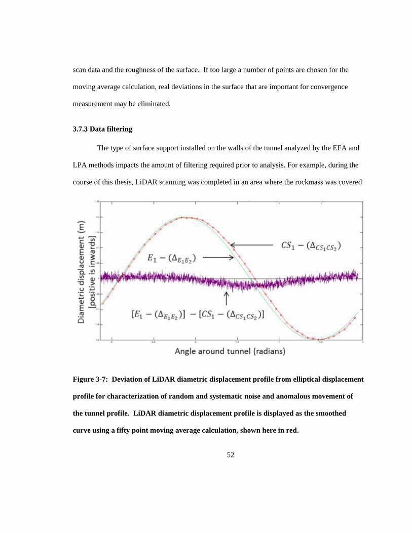
52
scan data and the roughness of the surface. If too large a number of points are chosen for the
moving average calculation, real deviations in the surface that are important for convergence
measurement may be eliminated.
3.7.3 Data filtering
The type of surface support installed on the walls of the tunnel analyzed by the EFA and
LPA methods impacts the amount of filtering required prior to analysis. For example, during the
course of this thesis, LiDAR scanning was completed in an area where the rockmass was covered
Figure 3-7: Deviation of LiDAR diametric displacement profile from elliptical displacement
profile for characterization of random and systematic noise and anomalous movement of
the tunnel profile. LiDAR diametric displacement profile is displayed as the smoothed
curve using a fifty point moving average calculation, shown here in red.
53
in steel screen. In this area the screen is the minimum level of support, and hence a necessary
safety precaution. Although screen presents additional challenges to using LiDAR scan data for
change detection, the use of LiDAR scanning is still effective. However, meshing of the LiDAR
data (seen in Figure 3-8), which includes the screen, introduces error into the final data set.
In order to remove the effect of the screen on the meshed data, the screen must be filtered
prior to meshing (Figure 3-9). Initially it was thought that it might be possible to filter the screen
out based on the intensity data collected by the LiDAR, but the results of the scanning show that
the difference between the intensity return of the mesh and the rock is negligible. A filter has
been included in the EFA and LPA that allows for near surface deviations from the rock profile
(such as screen) to be removed based on the distance from the center of the ellipse to the surface.
The user must choose the appropriate “look window” size and “filter cut-off” for filtration, based
on point spacing and the size of deviation to be removed. The “look window” is the portion of
the diameter of the tunnel to be filtered at a given time. The “filter cut-off” is the percentage of
the tunnel profile data to keep. For large anomalies (i.e. rockbolts) a large look window is
necessary. For near surface anomalies and rough profiles a smaller look window is best. Some
trial and error may be required to properly filter the surface.
3.8 Workflow
To further explain the process that the Elliptical Fit Analysis (EFA) and LiDAR Profile Analysis
(LPA) must follow, a workflow demonstrating the steps of the procedure has been created (Figure
3-10). As explained in sections 3.7.1 and 3.7.2, first two separate tunnel profiles are extracted
from the LiDAR data sets (Figure 3-10 a & b). Each of the extracted LiDAR tunnel profiles,
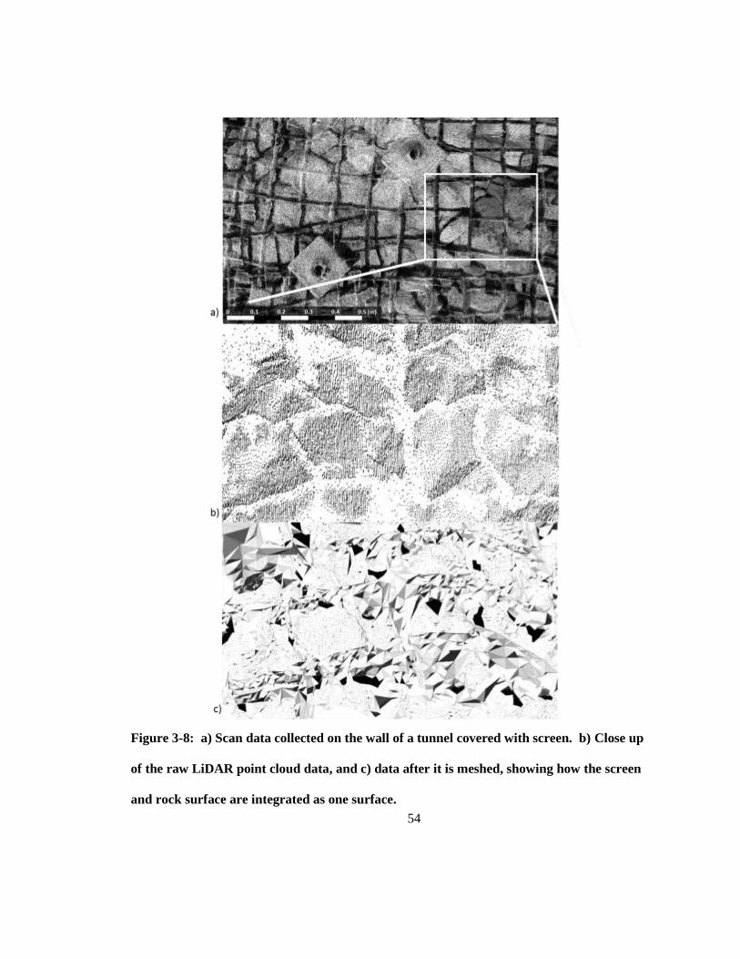
54
Figure 3-8: a) Scan data collected on the wall of a tunnel covered with screen. b) Close up
of the raw LiDAR point cloud data, and c) data after it is meshed, showing how the screen
and rock surface are integrated as one surface.
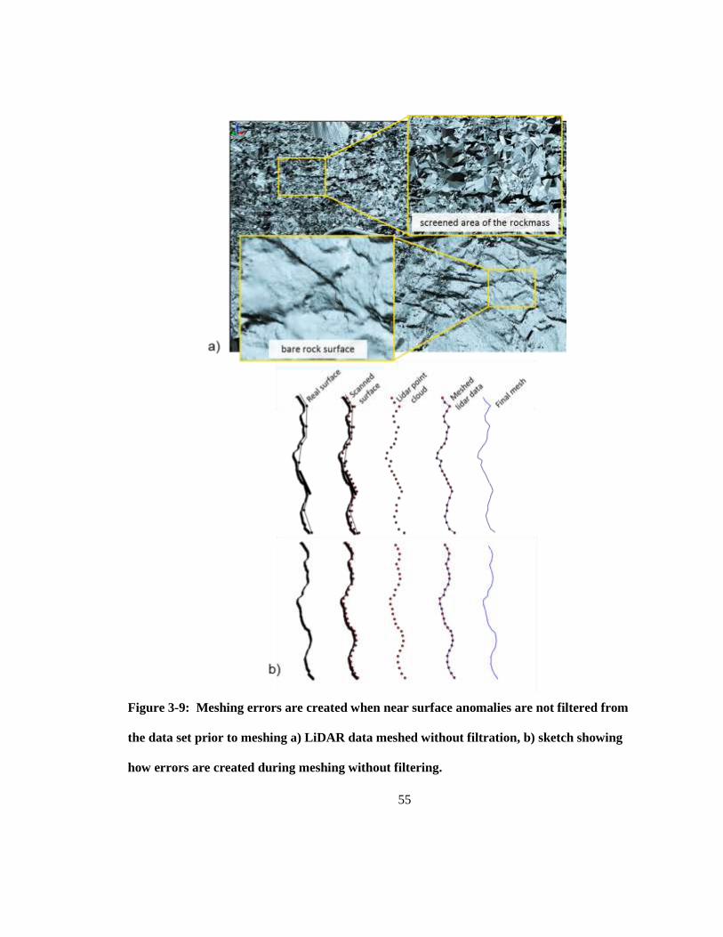
55
Figure 3-9: Meshing errors are created when near surface anomalies are not filtered from
the data set prior to meshing a) LiDAR data meshed without filtration, b) sketch showing
how errors are created during meshing without filtering.
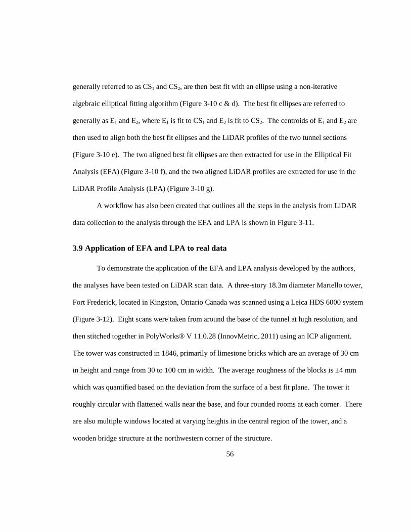
56
generally referred to as CS1 and CS2, are then best fit with an ellipse using a non-iterative
algebraic elliptical fitting algorithm (Figure 3-10 c & d). The best fit ellipses are referred to
generally as E1 and E2, where E1 is fit to CS1 and E2 is fit to CS2. The centroids of E1 and E2 are
then used to align both the best fit ellipses and the LiDAR profiles of the two tunnel sections
(Figure 3-10 e). The two aligned best fit ellipses are then extracted for use in the Elliptical Fit
Analysis (EFA) (Figure 3-10 f), and the two aligned LiDAR profiles are extracted for use in the
LiDAR Profile Analysis (LPA) (Figure 3-10 g).
A workflow has also been created that outlines all the steps in the analysis from LiDAR
data collection to the analysis through the EFA and LPA is shown in Figure 3-11.
3.9 Application of EFA and LPA to real data
To demonstrate the application of the EFA and LPA analysis developed by the authors,
the analyses have been tested on LiDAR scan data. A three-story 18.3m diameter Martello tower,
Fort Frederick, located in Kingston, Ontario Canada was scanned using a Leica HDS 6000 system
(Figure 3-12). Eight scans were taken from around the base of the tunnel at high resolution, and
then stitched together in PolyWorks® V 11.0.28 (InnovMetric, 2011) using an ICP alignment.
The tower was constructed in 1846, primarily of limestone bricks which are an average of 30 cm
in height and range from 30 to 100 cm in width. The average roughness of the blocks is ±4 mm
which was quantified based on the deviation from the surface of a best fit plane. The tower it
roughly circular with flattened walls near the base, and four rounded rooms at each corner. There
are also multiple windows located at varying heights in the central region of the tower, and a
wooden bridge structure at the northwestern corner of the structure.
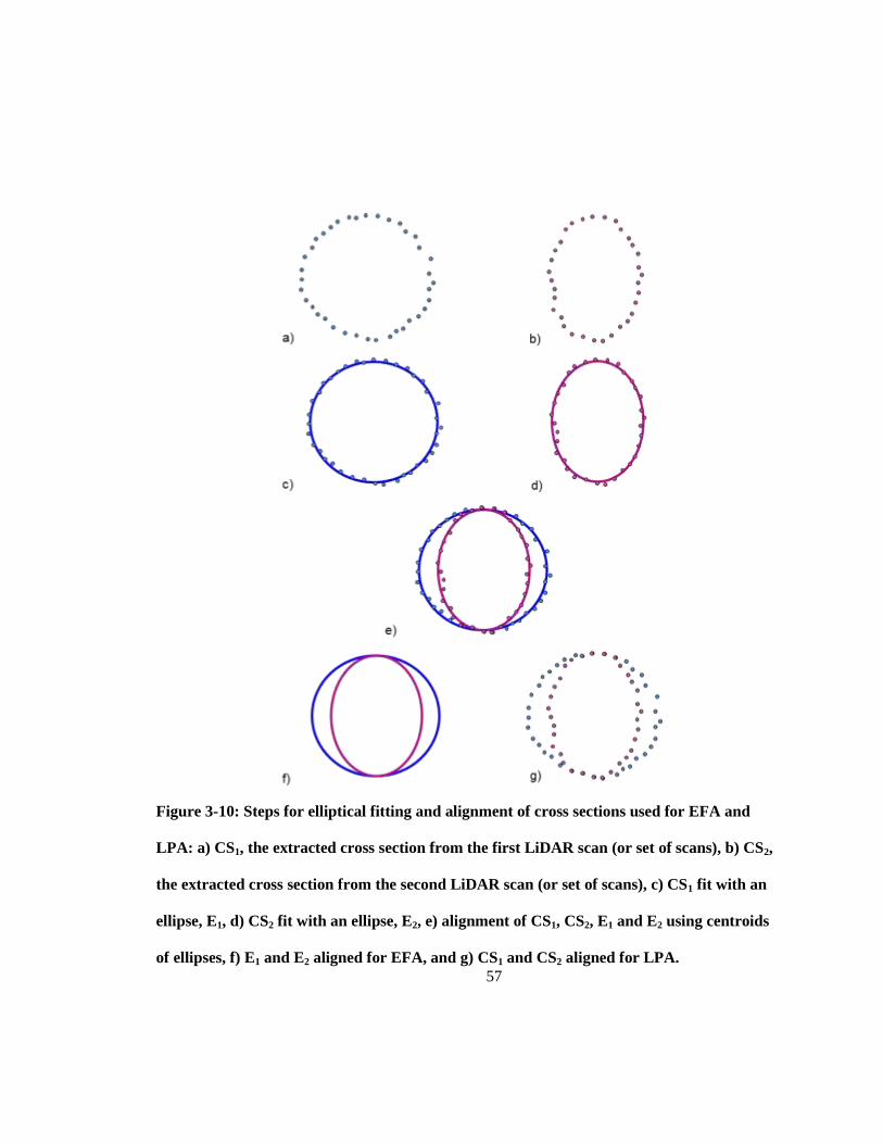
57
Figure 3-10: Steps for elliptical fitting and alignment of cross sections used for EFA and
LPA: a) CS1, the extracted cross section from the first LiDAR scan (or set of scans), b) CS2,
the extracted cross section from the second LiDAR scan (or set of scans), c) CS1 fit with an
ellipse, E1, d) CS2 fit with an ellipse, E2, e) alignment of CS1, CS2, E1 and E2 using centroids
of ellipses, f) E1 and E2 aligned for EFA, and g) CS1 and CS2 aligned for LPA.
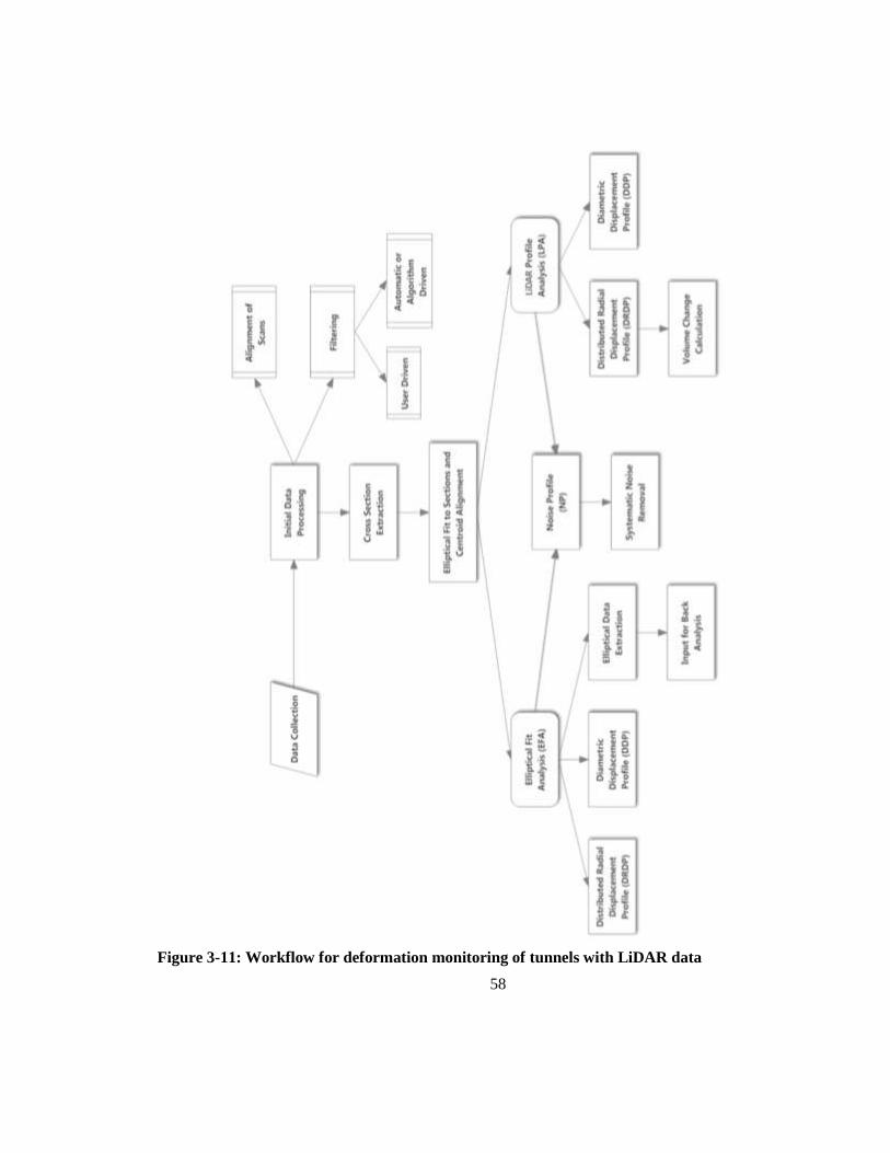
58
Figure 3-11: Workflow for deformation monitoring of tunnels with LiDAR data
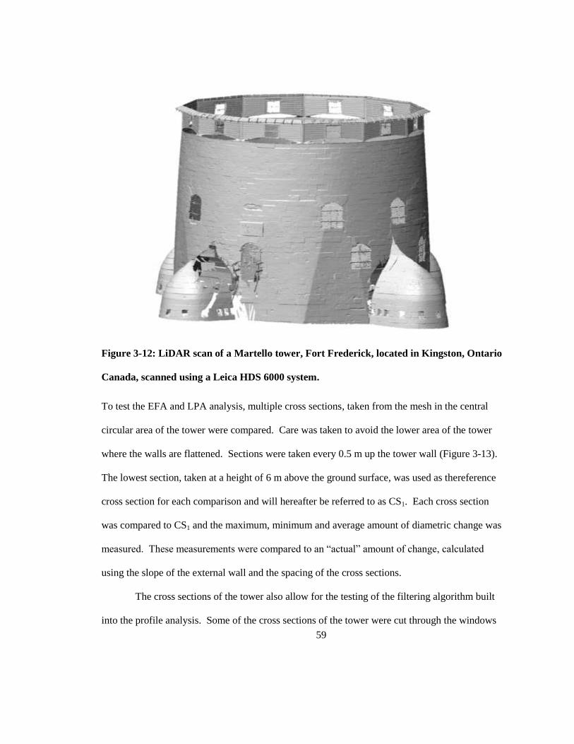
59
Figure 3-12: LiDAR scan of a Martello tower, Fort Frederick, located in Kingston, Ontario
Canada, scanned using a Leica HDS 6000 system.
To test the EFA and LPA analysis, multiple cross sections, taken from the mesh in the central
circular area of the tower were compared. Care was taken to avoid the lower area of the tower
where the walls are flattened. Sections were taken every 0.5 m up the tower wall (Figure 3-13).
The lowest section, taken at a height of 6 m above the ground surface, was used as thereference
cross section for each comparison and will hereafter be referred to as CS1. Each cross section
was compared to CS1 and the maximum, minimum and average amount of diametric change was
measured. These measurements were compared to an “actual” amount of change, calculated
using the slope of the external wall and the spacing of the cross sections.
The cross sections of the tower also allow for the testing of the filtering algorithm built
into the profile analysis. Some of the cross sections of the tower were cut through the windows
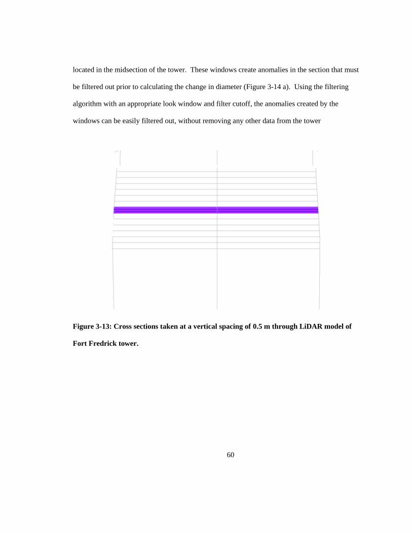
60
located in the midsection of the tower. These windows create anomalies in the section that must
be filtered out prior to calculating the change in diameter (Figure 3-14 a). Using the filtering
algorithm with an appropriate look window and filter cutoff, the anomalies created by the
windows can be easily filtered out, without removing any other data from the tower
Figure 3-13: Cross sections taken at a vertical spacing of 0.5 m through LiDAR model of
Fort Fredrick tower.
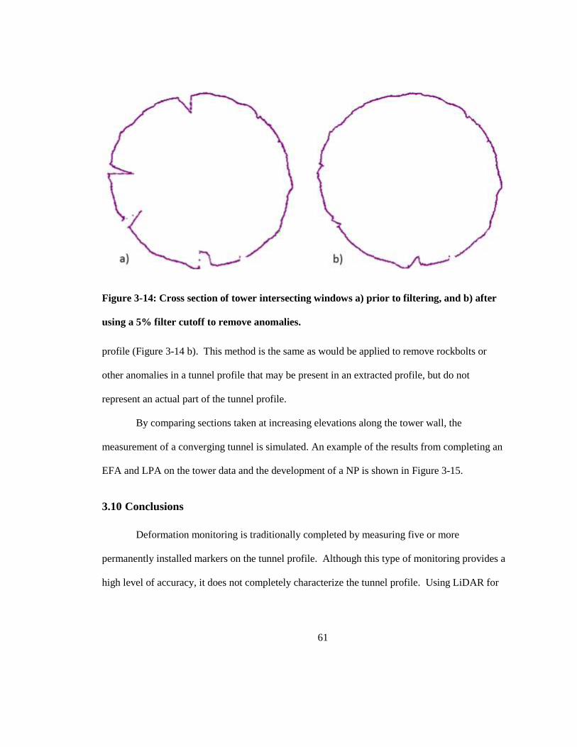
61
Figure 3-14: Cross section of tower intersecting windows a) prior to filtering, and b) after
using a 5% filter cutoff to remove anomalies.
profile (Figure 3-14 b). This method is the same as would be applied to remove rockbolts or
other anomalies in a tunnel profile that may be present in an extracted profile, but do not
represent an actual part of the tunnel profile.
By comparing sections taken at increasing elevations along the tower wall, the
measurement of a converging tunnel is simulated. An example of the results from completing an
EFA and LPA on the tower data and the development of a NP is shown in Figure 3-15.
3.10 Conclusions
Deformation monitoring is traditionally completed by measuring five or more
permanently installed markers on the tunnel profile. Although this type of monitoring provides a
high level of accuracy, it does not completely characterize the tunnel profile. Using LiDAR for

62
tunnel deformation monitoring provides the user with the ability to capture a much more
complete picture of the location and pattern of deformations occurring.
A new method for tunnel profile analysis using elliptical fitting to LiDAR profiles has been
developed to allow for analysis both of the general trends in deformation and for the analysis of
anomalous movements. General trends of deformation can found using the Elliptical Fit Analysis
(EFA) and can be used for back analysis of stresses and rockmass properties such as
deformability. Using LiDAR Profile Analysis (LPA), areas shown to be moving anomalously
can be analyzed separately from the general trends, and supported additionally to maintain
stability.
In the future it will be important to test the sensitivity of the newly developed EFA and
LPA to errors that occur within LiDAR data such as random noise, systematic noise, and
occlusion of the tunnel profile.
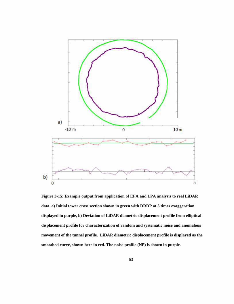
63
Figure 3-15: Example output from application of EFA and LPA analysis to real LiDAR
data. a) Initial tower cross section shown in green with DRDP at 5 times exaggeration
displayed in purple, b) Deviation of LiDAR diametric displacement profile from elliptical
displacement profile for characterization of random and systematic noise and anomalous
movement of the tunnel profile. LiDAR diametric displacement profile is displayed as the
smoothed curve, shown here in red. The noise profile (NP) is shown in purple.

64
65
Chapter 4
Sensitivity Testing of the Newly Developed Elliptical Fitting Method for
the Measurement of Convergence in Tunnels and Shafts2
4.1 Abstract
Light Detection and Ranging (LiDAR) is becoming more widely used in the geotechnical
community as its number of applications increase. It has been shown to be useful in tunneling for
applications such as rockmass characterization and discontinuity measurement. LiDAR data can
also be used to measure deformation in tunnels, but before a comprehensive methodology can be
developed, the accuracy issues associated with scanning must be fully understood. Once the
accuracy issues associated with LiDAR are well understood, any analysis technique that uses
LiDAR data must be tested to ensure the determined accuracy issues have minimal impact on the
results of the analysis.
To prove the usefulness of the newly developed elliptical fitting method for the
measurement of convergence in tunnels and shafts proposed by Delaloye et al. (2012), a
comprehensive analysis of accuracy issues associated with LiDAR scanning was conducted and
then a sensitivity test of the convergence measurement technique was completed. The results of
2 This chapter appears as submitted to an international journal with the following citation:
Delaloye, D., Hutchinson, J., Diederichs, M. (2012) Sensitivity Testing of the Newly Developed
Elliptical Fitting Method for the Measurement of Convergence in Tunnels and Shafts. Rock
Mechanics and Rock Engineering.
66
the analysis show that by using the statistical techniques built into the Elliptical Fit Analysis
(EFA) and LiDAR Profile Analysis (LPA), levels of change within the level of random and
systematic noise included in the data can be measured. Furthermore, the new analysis is robust
enough to handle large amounts of occlusion within data sets.
4.2 Introduction
Deformation monitoring is an important part of any underground excavation project.
Traditional monitoring generally involves measurement of either tapes or control points installed
around the perimeter of the excavation. Light Detection and Ranging (LiDAR) is becoming more
widely used in the geotechnical community, especially in underground environments, and there is
growing interest in its application to change detection and deformation monitoring. As
techniques for using LiDAR for deformation monitoring are developed, it is important they are
tested to ensure they can accurately characterize and measure change within an environment. To
do so, the accuracy issues associated with LiDAR scanning must be well understood and
techniques must be tested for their sensitivity to these accuracy issues.
This paper provides an in depth review of accuracy issues associated with LiDAR
scanning, and then tests the newly developed Elliptical Fit Analysis (EFA) and LiDAR Profile
Analysis (LPA) (Delaloye et al., 2012) for their sensitivity to these accuracy issues.
4.3 Deformation monitoring in tunnels
Deformation in tunnels occurs as a result of the redistribution of stress around the
excavation. The magnitude of deformation is related to the rockmass conditions, the stress ratio
and orientation, the excavation method, the rate of excavation, the type of support, and the

67
locations and distance from the face at which support is installed. Monitoring deformation of
tunnels is an important part of modern design and construction practices, and is the basis for the
New Austrian Tunneling Method (NATM) (Wittke et al., 2006). When using the NATM method
for tunnel excavation, if measurements of deformation are not consistent with those allowed for
in the initial support design, more support or different excavation methods are implemented.
Other benefits of deformation monitoring are:
deformation measurements can help refine the final liner design,
deformations can serve as an early warning for more severe failures, and
deformations can be used for back calculation of stress orientation and rockmass
properties.
4.3.1 Traditional monitoring techniques
Current techniques for monitoring deformation in tunnels involve one or more of the
following techniques (Kontogianni, 2003):
Tape extensometers
Geodetic surveys (ie. Total station)
Photogrammetric devices
Tape extensometers are the most accurate of the surveying devices listed. They have an
accuracy of +/- 0.2 mm over 10-15 m (Kavvadas, 2005). The main drawback with tape
extensometers is that they only have the ability to measure along a specific line between anchor
points which must be installed in the tunnel walls. The installation of permanent anchors often
interrupts the construction process of the tunnel. In addition, the anchor points are installed at a
time in the construction cycle when it is safe to access the excavation, which is usually after some
68
level of support has been installed. Therefore the monitoring commences at some distance back
from the advancing tunnel face. At this point, a significant portion of the tunnel deformation has
generally already occurred.
Total stations make use of optical reflectors installed around the tunnel profile (usually
five to seven points), as well as a stable reference point outside the zone of deformation, to
measure deformations. The station must be moved progressively forward from the area with the
stable reference points towards the locations of the tunnel profile of interest. A total station has
an accuracy of about +/- 2.5 mm over 100 m (Kavvadas, 2005). Total station reflectors are very
susceptible to disturbance and destruction during construction processes.
Photogrammetric devices require that a number of reference points be installed on the
surface of the tunnel. Photogrammetric devices, where the scanner is located using a total station,
have an accuracy of at worst +/- 5 mm (Kavvadas, 2005) but with new developments the
accuracy of these systems is increasing to the sub millimeter level.
4.4 Terrestrial laser scanning
LiDAR is a laser scanning technology used for quick acquisition of a dense point cloud
of three dimensional position data. LiDAR scanners can collect millions of points that have both
high accuracy, high precision positional data (x,y,z) and uncalibrated intensity values (i), in a
matter of minutes. For example, the Leica HDS 6000 (the scanner used for this research) collects
up to 500,000 points per second with a single point positional accuracy of 6mm at 1 m to 25 m,
and 10 mm at 50 m (Leica Geosystems, 2007) (measurements are one standard deviation). Newer
scanners can collect one million points per second, have increased accuracy, and include
additional features such as the ability to collect RGB color data for every point.
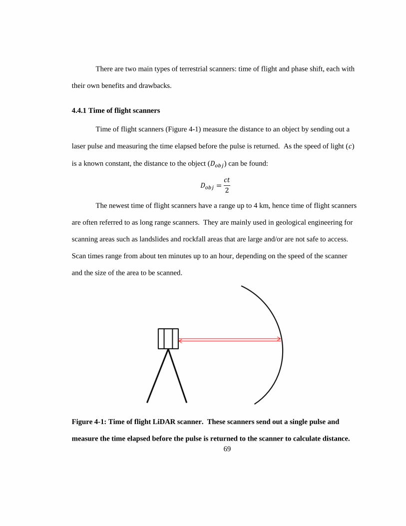
69
There are two main types of terrestrial scanners: time of flight and phase shift, each with
their own benefits and drawbacks.
4.4.1 Time of flight scanners
Time of flight scanners (Figure 4-1) measure the distance to an object by sending out a
laser pulse and measuring the time elapsed before the pulse is returned. As the speed of light ( )
is a known constant, the distance to the object ( ) can be found:
The newest time of flight scanners have a range up to 4 km, hence time of flight scanners
are often referred to as long range scanners. They are mainly used in geological engineering for
scanning areas such as landslides and rockfall areas that are large and/or are not safe to access.
Scan times range from about ten minutes up to an hour, depending on the speed of the scanner
and the size of the area to be scanned.
Figure 4-1: Time of flight LiDAR scanner. These scanners send out a single pulse and
measure the time elapsed before the pulse is returned to the scanner to calculate distance.
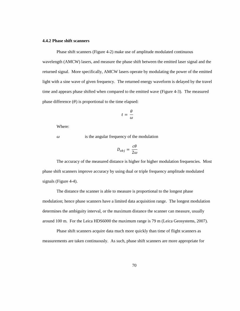
70
4.4.2 Phase shift scanners
Phase shift scanners (Figure 4-2) make use of amplitude modulated continuous
wavelength (AMCW) lasers, and measure the phase shift between the emitted laser signal and the
returned signal. More specifically, AMCW lasers operate by modulating the power of the emitted
light with a sine wave of given frequency. The returned energy waveform is delayed by the travel
time and appears phase shifted when compared to the emitted wave (Figure 4-3). The measured
phase difference ( ) is proportional to the time elapsed:
Where:
is the angular frequency of the modulation
The accuracy of the measured distance is higher for higher modulation frequencies. Most
phase shift scanners improve accuracy by using dual or triple frequency amplitude modulated
signals (Figure 4-4).
The distance the scanner is able to measure is proportional to the longest phase
modulation; hence phase scanners have a limited data acquisition range. The longest modulation
determines the ambiguity interval, or the maximum distance the scanner can measure, usually
around 100 m. For the Leica HDS6000 the maximum range is 79 m (Leica Geosystems, 2007).
Phase shift scanners acquire data much more quickly than time of flight scanners as
measurements are taken continuously. As such, phase shift scanners are more appropriate for
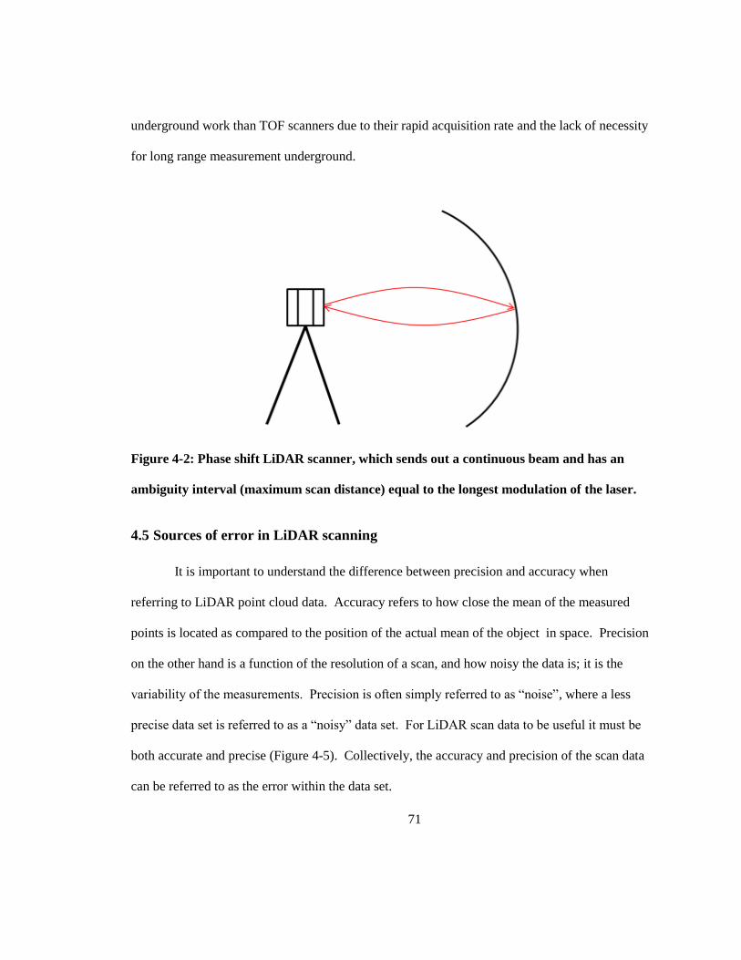
71
underground work than TOF scanners due to their rapid acquisition rate and the lack of necessity
for long range measurement underground.
Figure 4-2: Phase shift LiDAR scanner, which sends out a continuous beam and has an
ambiguity interval (maximum scan distance) equal to the longest modulation of the laser.
4.5 Sources of error in LiDAR scanning
It is important to understand the difference between precision and accuracy when
referring to LiDAR point cloud data. Accuracy refers to how close the mean of the measured
points is located as compared to the position of the actual mean of the object in space. Precision
on the other hand is a function of the resolution of a scan, and how noisy the data is; it is the
variability of the measurements. Precision is often simply referred to as “noise”, where a less
precise data set is referred to as a “noisy” data set. For LiDAR scan data to be useful it must be
both accurate and precise (Figure 4-5). Collectively, the accuracy and precision of the scan data
can be referred to as the error within the data set.
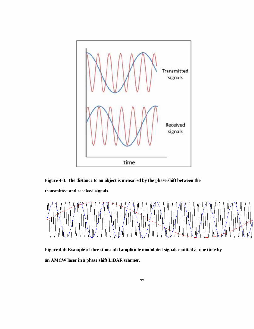
72
Figure 4-3: The distance to an object is measured by the phase shift between the
transmitted and received signals.
Figure 4-4: Example of thee sinusoidal amplitude modulated signals emitted at one time by
an AMCW laser in a phase shift LiDAR scanner.
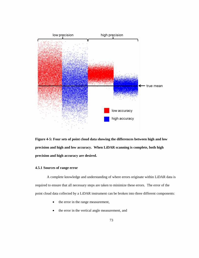
73
Figure 4-5: Four sets of point cloud data showing the differences between high and low
precision and high and low accuracy. When LiDAR scanning is complete, both high
precision and high accuracy are desired.
4.5.1 Sources of range error
A complete knowledge and understanding of where errors originate within LiDAR data is
required to ensure that all necessary steps are taken to minimize these errors. The error of the
point cloud data collected by a LiDAR instrument can be broken into three different components:
the error in the range measurement,
the error in the vertical angle measurement, and
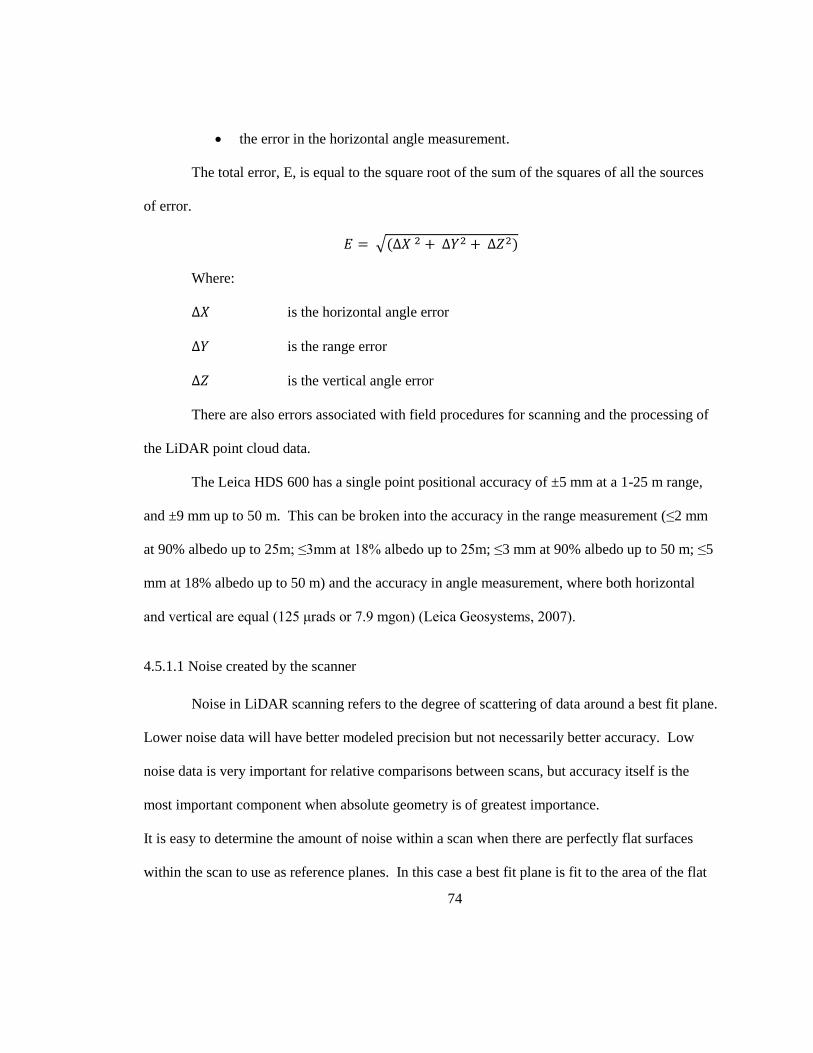
74
the error in the horizontal angle measurement.
The total error, E, is equal to the square root of the sum of the squares of all the sources
of error.
√( )
Where:
is the horizontal angle error
is the range error
is the vertical angle error
There are also errors associated with field procedures for scanning and the processing of
the LiDAR point cloud data.
The Leica HDS 600 has a single point positional accuracy of ±5 mm at a 1-25 m range,
and ±9 mm up to 50 m. This can be broken into the accuracy in the range measurement (≤2 mm
at 90% albedo up to 25m; ≤3mm at 18% albedo up to 25m; ≤3 mm at 90% albedo up to 50 m; ≤5
mm at 18% albedo up to 50 m) and the accuracy in angle measurement, where both horizontal
and vertical are equal (125 μrads or 7.9 mgon) (Leica Geosystems, 2007).
4.5.1.1 Noise created by the scanner
Noise in LiDAR scanning refers to the degree of scattering of data around a best fit plane.
Lower noise data will have better modeled precision but not necessarily better accuracy. Low
noise data is very important for relative comparisons between scans, but accuracy itself is the
most important component when absolute geometry is of greatest importance.
It is easy to determine the amount of noise within a scan when there are perfectly flat surfaces
within the scan to use as reference planes. In this case a best fit plane is fit to the area of the flat
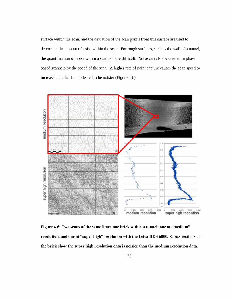
75
surface within the scan, and the deviation of the scan points from this surface are used to
determine the amount of noise within the scan. For rough surfaces, such as the wall of a tunnel,
the quantification of noise within a scan is more difficult. Noise can also be created in phase
based scanners by the speed of the scan. A higher rate of point capture causes the scan speed to
increase, and the data collected to be noisier (Figure 4-6).
Figure 4-6: Two scans of the same limestone brick within a tunnel: one at “medium”
resolution, and one at “super high” resolution with the Leica HDS 6000. Cross sections of
the brick show the super high resolution data is noisier than the medium resolution data.
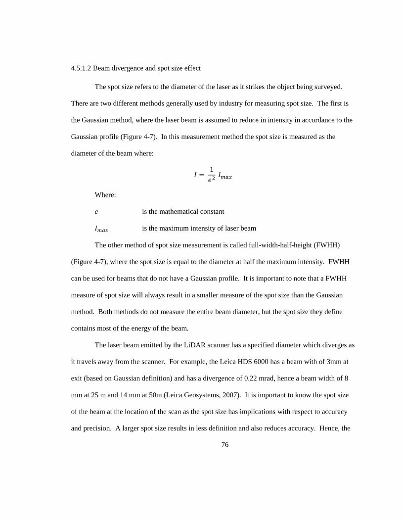
76
4.5.1.2 Beam divergence and spot size effect
The spot size refers to the diameter of the laser as it strikes the object being surveyed.
There are two different methods generally used by industry for measuring spot size. The first is
the Gaussian method, where the laser beam is assumed to reduce in intensity in accordance to the
Gaussian profile (Figure 4-7). In this measurement method the spot size is measured as the
diameter of the beam where:
Where:
e is the mathematical constant
is the maximum intensity of laser beam
The other method of spot size measurement is called full-width-half-height (FWHH)
(Figure 4-7), where the spot size is equal to the diameter at half the maximum intensity. FWHH
can be used for beams that do not have a Gaussian profile. It is important to note that a FWHH
measure of spot size will always result in a smaller measure of the spot size than the Gaussian
method. Both methods do not measure the entire beam diameter, but the spot size they define
contains most of the energy of the beam.
The laser beam emitted by the LiDAR scanner has a specified diameter which diverges as
it travels away from the scanner. For example, the Leica HDS 6000 has a beam with of 3mm at
exit (based on Gaussian definition) and has a divergence of 0.22 mrad, hence a beam width of 8
mm at 25 m and 14 mm at 50m (Leica Geosystems, 2007). It is important to know the spot size
of the beam at the location of the scan as the spot size has implications with respect to accuracy
and precision. A larger spot size results in less definition and also reduces accuracy. Hence, the
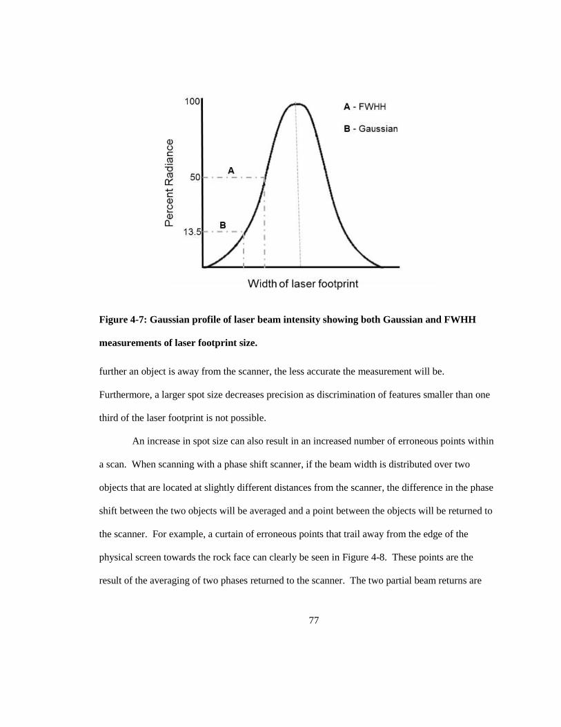
77
Figure 4-7: Gaussian profile of laser beam intensity showing both Gaussian and FWHH
measurements of laser footprint size.
further an object is away from the scanner, the less accurate the measurement will be.
Furthermore, a larger spot size decreases precision as discrimination of features smaller than one
third of the laser footprint is not possible.
An increase in spot size can also result in an increased number of erroneous points within
a scan. When scanning with a phase shift scanner, if the beam width is distributed over two
objects that are located at slightly different distances from the scanner, the difference in the phase
shift between the two objects will be averaged and a point between the objects will be returned to
the scanner. For example, a curtain of erroneous points that trail away from the edge of the
physical screen towards the rock face can clearly be seen in Figure 4-8. These points are the
result of the averaging of two phases returned to the scanner. The two partial beam returns are
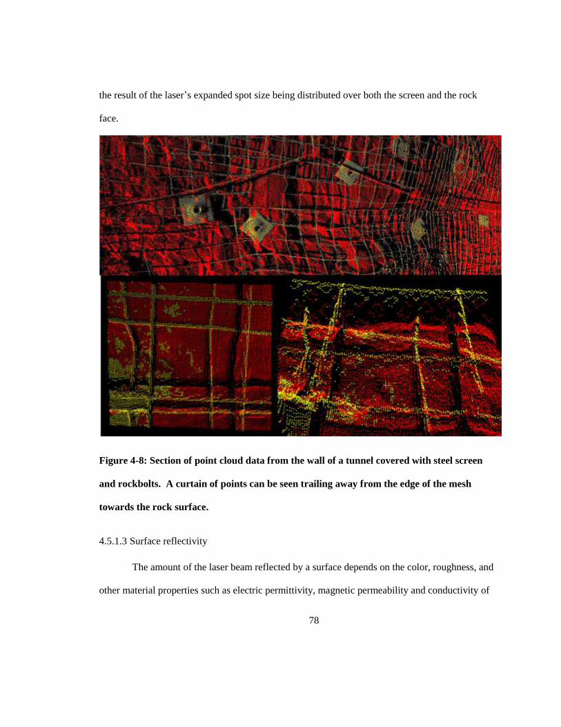
78
the result of the laser’s expanded spot size being distributed over both the screen and the rock
face.
Figure 4-8: Section of point cloud data from the wall of a tunnel covered with steel screen
and rockbolts. A curtain of points can be seen trailing away from the edge of the mesh
towards the rock surface.
4.5.1.3 Surface reflectivity
The amount of the laser beam reflected by a surface depends on the color, roughness, and
other material properties such as electric permittivity, magnetic permeability and conductivity of
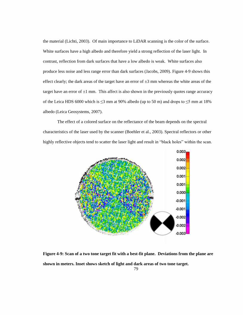
79
the material (Lichti, 2003). Of main importance to LiDAR scanning is the color of the surface.
White surfaces have a high albedo and therefore yield a strong reflection of the laser light. In
contrast, reflection from dark surfaces that have a low albedo is weak. White surfaces also
produce less noise and less range error than dark surfaces (Jacobs, 2009). Figure 4-9 shows this
effect clearly; the dark areas of the target have an error of ±3 mm whereas the white areas of the
target have an error of ±1 mm. This affect is also shown in the previously quotes range accuracy
of the Leica HDS 6000 which is ≤3 mm at 90% albedo (up to 50 m) and drops to ≤5 mm at 18%
albedo (Leica Geosystems, 2007).
The effect of a colored surface on the reflectance of the beam depends on the spectral
characteristics of the laser used by the scanner (Boehler et al., 2003). Spectral reflectors or other
highly reflective objects tend to scatter the laser light and result in “black holes” within the scan.
Figure 4-9: Scan of a two tone target fit with a best-fit plane. Deviations from the plane are
shown in meters. Inset shows sketch of light and dark areas of two tone target.
80
4.5.1.4 Scan density and spatial resolution
The scan density is a measure of how close the point spacing is in a given scan. For a
phase based scanner the density is based on the frequency of the beam of the continuous laser
source. Scan density can be increased either by sampling more frequently, or, where this is not an
option, multiple scans can be done of the same area. In general, a higher scan density results in a
higher resolution of the scan. The point spacing also increases as a function of distance from the
scanner.
It is essential to know the spatial resolution of the scanner before acquiring scan data to
determine the level of detail that can be resolved from the data. There are different methods for
determining spatial resolution of a scanner. Lichti & Jamtsho (2006) proposed the effective
instantaneous field of view (EIFOV), which more suppliers are moving towards for measuring
resolution. The EIFOV is a function of the sampling density, the width of the laser beam (spot
size) and the angle of incidence between the scanner and the surface being scanned. Traditionally
an angular resolution and a range resolution are provided. A full explanation on how to measure
resolution is beyond the scope of this paper, but the important issue to note is that resolution
defines the smallest data sampling range-interval that can be extracted from data.
4.5.1.5 Angle of incidence
The angle at which the laser hits the object being scanned will affect the accuracy of the
scan. At an angle of incidence perpendicular to the scanner, the accuracy of the data collected is
greatest. As the angle increases and the scanned surface becomes more oblique to the scanner,
the measurement of the object’s position becomes less accurate. Higher incidence angles and
longer distances result in high noise levels (Soudarissanane et al., 2007, Lato, 2010). Data
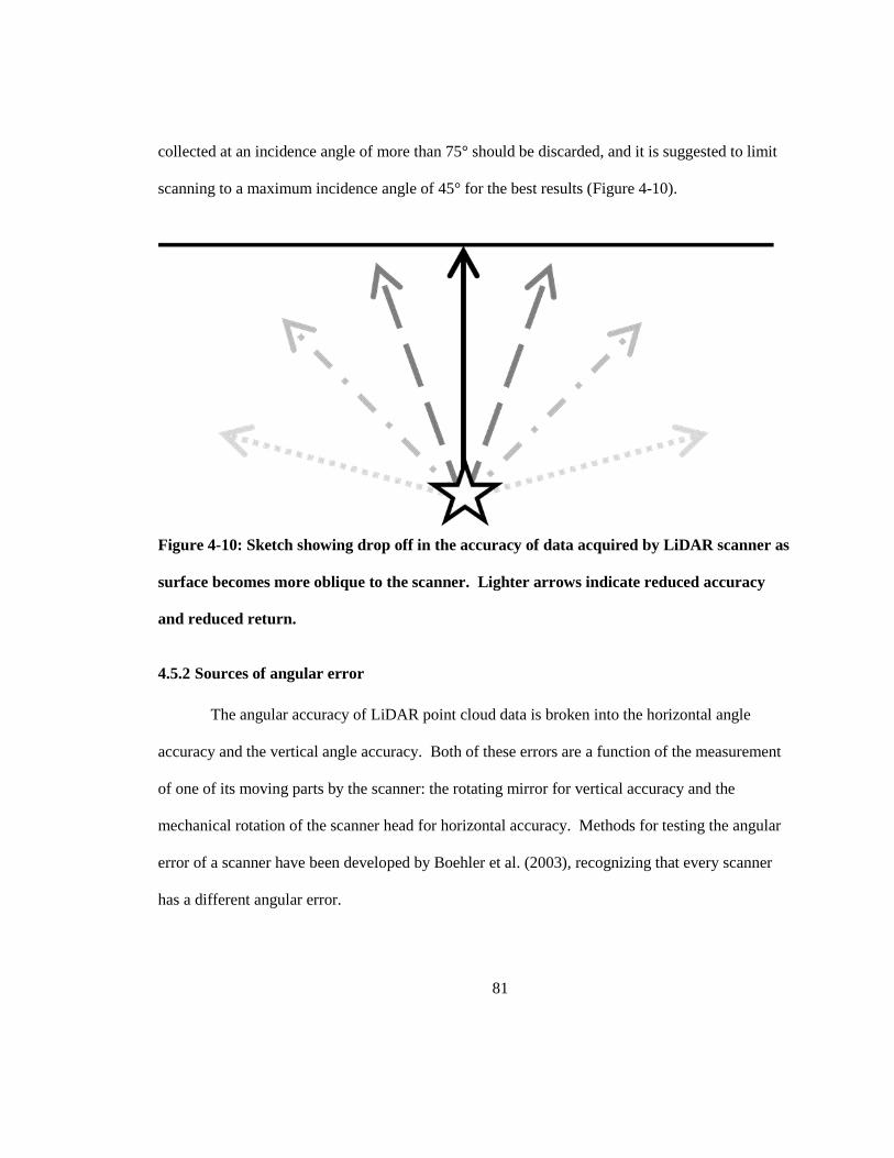
81
collected at an incidence angle of more than 75° should be discarded, and it is suggested to limit
scanning to a maximum incidence angle of 45° for the best results (Figure 4-10).
Figure 4-10: Sketch showing drop off in the accuracy of data acquired by LiDAR scanner as
surface becomes more oblique to the scanner. Lighter arrows indicate reduced accuracy
and reduced return.
4.5.2 Sources of angular error
The angular accuracy of LiDAR point cloud data is broken into the horizontal angle
accuracy and the vertical angle accuracy. Both of these errors are a function of the measurement
of one of its moving parts by the scanner: the rotating mirror for vertical accuracy and the
mechanical rotation of the scanner head for horizontal accuracy. Methods for testing the angular
error of a scanner have been developed by Boehler et al. (2003), recognizing that every scanner
has a different angular error.

82
It is important to ensure that the scanner used for collection of LiDAR data is calibrated
correctly as this is the only way to minimize angular error. If a scanner is not calibrated correctly,
accuracy of the scan data will be reduced.
4.5.3 Other sources of error
4.5.3.1 Spurious scan points
Spurious scan points are points within a LiDAR point cloud that do not represent any real
object within the scan. These points should not have been collected by the scanner and must be
removed by the user or through a filter before the scan data can be used for deformation
monitoring. There are many conditions that can result in spurious points which include, but are
not limited to, atmospheric conditions, interfering radiation, reflective surfaces, edge effects, and
the ambiguity interval of the scanner.
Atmospheric conditions such as dust or steam in the air can result in unwanted return
points. Dust and vapor can scatter the laser, either increasing the noise upon return or returning
spurious points. Interfering radiation such as the rays of the sun, which have a similar
wavelength to that of the scanner, can be picked up as spurious points. Reflective surfaces such
as mirrors or wet surfaces can reflect the laser beam. The beams will be returned from locations
other than where they initially hit the object.
4.5.3.2 Ambiguity interval
Every phase based laser scanner has a stated ambiguity interval, beyond which distance
the phase shift of the returned beam is ambiguous. If points are returned to the laser scanner from
a distance farther than the ambiguity interval they will be positioned too close to the scanner. For
83
example, if the ambiguity interval of a scanner is 60 m and a point is returned from 62 m it will
be stored as being 2 m away from the scanner.
4.5.3.3 Georeferencing and alignment error
Error associated with the georeferencing of a LiDAR scan is based on the error in the
georeferencing measurements. The less error in the georeferencing measurements used to align
the scan, the less error in the scan itself. Error in a scan can also be created if it is not aligned
properly with other scans, or if it is aligned with a scan that is poorly georeferenced.
4.6 Sources of noise in tunneling
There are other sources of noise when scanning in a tunneling environment that are not
associated with the LiDAR scanning itself. The first of these sources of noise is the roughness of
the tunnel profile. This roughness can be broken into two different components: the roughness
associated with the rock surface (generally a combination of the rock type and the excavation
method and quality) and the roughness or systematic undulation caused by rock structures and
other large (macro) scale features. Both of these sources of noise are unavoidable, and can vary
drastically from one section of tunnel to another. It is important that any type of profile analysis
for a tunnel be able to deal with these sources of noise. Random noise is generally considered to
have a maximum centimeter scale magnitude, whereas systematic undulation of the profile can be
up to meters in scale.
Another unavoidable source of noise within a tunneling environment is occlusion. When
scanning in a tunneling environment, occlusion of part of the tunnel profile is generally
unavoidable. Machinery, ventilation ducts, conveyor systems, tunneling equipment or workers in
84
the tunnel may obstruct the LiDAR scanner from collecting parts of the walls or roofs in the
tunnel. These obstructions are most likely to be encountered in tunnels that are under
construction, where convergence measurement is more important. For a convergence
measurement technique to be effective, the analysis must be able to deal with partially occluded
data sets.
4.7 Positioning in LiDAR scanning
When completing a LiDAR scanning program it is important to decide in advance what
reference system will be used for alignment of scan data. Either absolute positioning or relative
positioning can be used. Absolute positioning can be completed using GPS data of specific
reference points within the scan, or by surveying in the laser scanner using a device such as a
total station. Although it is often assumed that absolute positioning is necessary to characterize
deformation, this is not the case. Using relative convergence provides the same level of stability
information and back analysis ability as using absolute positioning measurement. The main
limitation with not having absolute positioning data is that no lateral or vertical movement of the
tunnel can be tracked, but these types of movement typically are only of concern in twin bore
tunnels at depth.
4.8 Tunnel profile analysis with LiDAR data using elliptical fitting
Terzaghi (1942) introduced a method to fit an ellipse to the displaced points monitored in
a tunnel. His calculation of the mean deformation ellipse replaced the traditional method of
looking at each point individually. The mean deformation ellipse allows for different periods of
deformation to be easily characterized. For example, one can discern periods of vertical and
85
horizontal compression much more clearly than by looking at each point by itself (Stiros &
Kontogianni, 2009). To apply Terzaghi’s method of elliptical fitting, a new method for analyzing
LiDAR data has been developed. The analysis comprises a combined Elliptical Fit Analysis
(EFA) and LiDAR Profile Analysis (LPA) described in detail by Delaloye et al. (2012) (Figure
4-11).
4.8.1 Generating synthetic LiDAR tunnel profiles
To test the new methodology for profile analysis a synthetic LiDAR profile data
generator was created. The use of synthetic data allows for the amount of deformation that is
measured by the analysis to be compared to the amount of deformation that is mathematically
included in the data. Once the new methodology, the combined EFA and LPA, is proved useful
and its limitations defined using the synthetic data, it can be applied to real LiDAR scan data.
The synthetic data generator, created in Matlab as part of this thesis, allows for selection
of the number of points (which are evenly spatially distributed) and for the radius of the tunnel
profile to be chosen. Both random uncorrelated noise with a defined standard deviation and
systematic noise (locally consistent deviation from the elliptical profile) can be added to the data
(Figure 4-12 b, c).
Data can also be “elliptically skewed”: the short axis of the tunnel profile is contracted
and the long axis of the profile is expanded radially by the amount of “skew” entered by the user
(Figure 4-12 d). The new elliptical data set can then be rotated to simulate directions of minimum
and maximum deformation that are not parallel to the x and y axis.
The generated tunnel profile data can also be occluded to simulate data that cannot be
collected within a tunneling environment due to ventilation, machinery, workers, and other
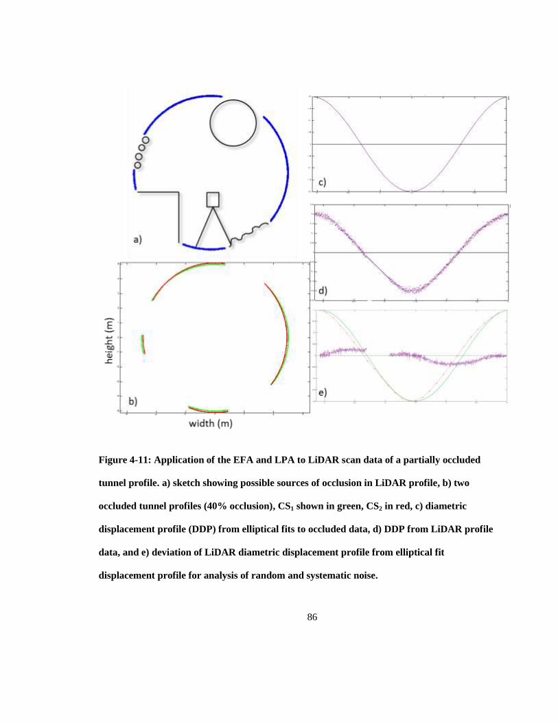
86
Figure 4-11: Application of the EFA and LPA to LiDAR scan data of a partially occluded
tunnel profile. a) sketch showing possible sources of occlusion in LiDAR profile, b) two
occluded tunnel profiles (40% occlusion), CS1 shown in green, CS2 in red, c) diametric
displacement profile (DDP) from elliptical fits to occluded data, d) DDP from LiDAR profile
data, and e) deviation of LiDAR diametric displacement profile from elliptical fit
displacement profile for analysis of random and systematic noise.
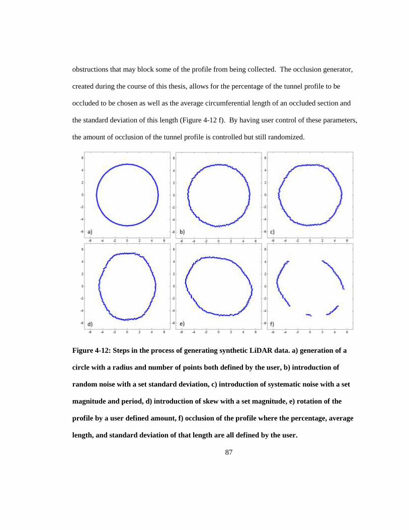
87
obstructions that may block some of the profile from being collected. The occlusion generator,
created during the course of this thesis, allows for the percentage of the tunnel profile to be
occluded to be chosen as well as the average circumferential length of an occluded section and
the standard deviation of this length (Figure 4-12 f). By having user control of these parameters,
the amount of occlusion of the tunnel profile is controlled but still randomized.
Figure 4-12: Steps in the process of generating synthetic LiDAR data. a) generation of a
circle with a radius and number of points both defined by the user, b) introduction of
random noise with a set standard deviation, c) introduction of systematic noise with a set
magnitude and period, d) introduction of skew with a set magnitude, e) rotation of the
profile by a user defined amount, f) occlusion of the profile where the percentage, average
length, and standard deviation of that length are all defined by the user.
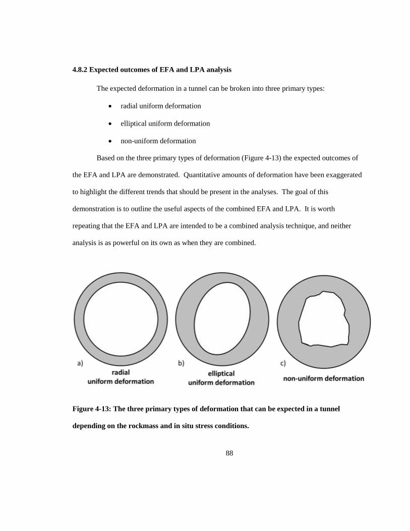
88
4.8.2 Expected outcomes of EFA and LPA analysis
The expected deformation in a tunnel can be broken into three primary types:
radial uniform deformation
elliptical uniform deformation
non-uniform deformation
Based on the three primary types of deformation (Figure 4-13) the expected outcomes of
the EFA and LPA are demonstrated. Quantitative amounts of deformation have been exaggerated
to highlight the different trends that should be present in the analyses. The goal of this
demonstration is to outline the useful aspects of the combined EFA and LPA. It is worth
repeating that the EFA and LPA are intended to be a combined analysis technique, and neither
analysis is as powerful on its own as when they are combined.
Figure 4-13: The three primary types of deformation that can be expected in a tunnel
depending on the rockmass and in situ stress conditions.

89
4.8.2.1 Radial uniform deformation
Under hydrostatic stress conditions in homogeneous isotropic rock, radial uniform
deformation of the rockmass (Figure 4-13 a) is expected. Radial uniform deformation is
characterized by a near equal displacement of the tunnel wall at every point. The Distributed
Radial Displacement Profile (DRDP) and Diametric Displacement Profile (DDP) from the EFA
and the LPA, as well as the Noise Profile (NP) are shown in Figure 4-14 for a tunnel undergoing
this type of deformation. If a tunnel is undergoing radial uniform deformation both the DDP
from the EFA and the DDP from the LPA should be flat lines equal to the amount of diametric
convergence, as deformation is consistent around the tunnel profile. There should be no deviation
between the DDPs, therefore the NP should also be flat, which is consistent with the results
shown in Figure 4-14 g.
4.8.2.2 Elliptical uniform deformation
Elliptical uniform deformation (Figure 4-13b) can be expected in a rockmass when either
the stress conditions are non-homogeneous, or the rockmass is anisotropic. The output of the
EFA and LPA analysis for a tunnel profile undergoing elliptical uniform deformation is shown in
Figure 4-15. Both the DRDP from the EFA and LPA show the same pattern of deformation, an
exaggerated “peanut” shape characteristic of an elliptical deformation tensor. The DDP of both
analyses is a sinusoidal wave characteristic of elliptical deformation. The NP shows that the
elliptical fit and the LiDAR profile provide similar DDPs, but there is a small amount of
discrepancy. This discrepancy is associated with the fact that the LiDAR profile is not perfectly
elliptical, not that anomalous movement is occurring.
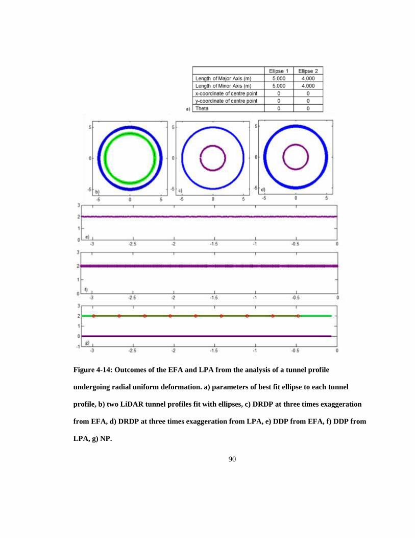
90
Figure 4-14: Outcomes of the EFA and LPA from the analysis of a tunnel profile
undergoing radial uniform deformation. a) parameters of best fit ellipse to each tunnel
profile, b) two LiDAR tunnel profiles fit with ellipses, c) DRDP at three times exaggeration
from EFA, d) DRDP at three times exaggeration from LPA, e) DDP from EFA, f) DDP from
LPA, g) NP.
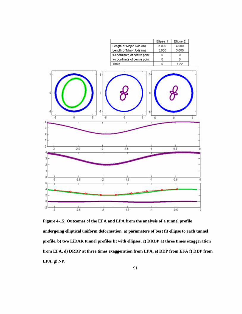
91
Figure 4-15: Outcomes of the EFA and LPA from the analysis of a tunnel profile
undergoing elliptical uniform deformation. a) parameters of best fit ellipse to each tunnel
profile, b) two LiDAR tunnel profiles fit with ellipses, c) DRDP at three times exaggeration
from EFA, d) DRDP at three times exaggeration from LPA, e) DDP from EFA f) DDP from
LPA, g) NP.
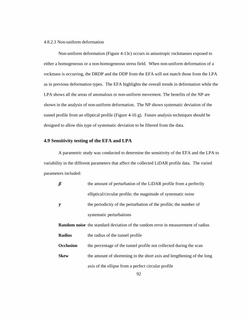
92
4.8.2.3 Non-uniform deformation
Non-uniform deformation (Figure 4-13c) occurs in anisotropic rockmasses exposed to
either a homogeneous or a non-homogeneous stress field. When non-uniform deformation of a
rockmass is occurring, the DRDP and the DDP from the EFA will not match those from the LPA
as in previous deformation types. The EFA highlights the overall trends in deformation while the
LPA shows all the areas of anomalous or non-uniform movement. The benefits of the NP are
shown in the analysis of non-uniform deformation. The NP shows systematic deviation of the
tunnel profile from an elliptical profile (Figure 4-16 g). Future analysis techniques should be
designed to allow this type of systematic deviation to be filtered from the data.
4.9 Sensitivity testing of the EFA and LPA
A parametric study was conducted to determine the sensitivity of the EFA and the LPA to
variability in the different parameters that affect the collected LiDAR profile data. The varied
parameters included:
the amount of perturbation of the LiDAR profile from a perfectly
elliptical/circular profile; the magnitude of systematic noise
the periodicity of the perturbation of the profile; the number of
systematic perturbations
Random noise the standard deviation of the random error in measurement of radius
Radius the radius of the tunnel profile
Occlusion the percentage of the tunnel profile not collected during the scan
Skew the amount of shortening in the short axis and lengthening of the long
axis of the ellipse from a perfect circular profile
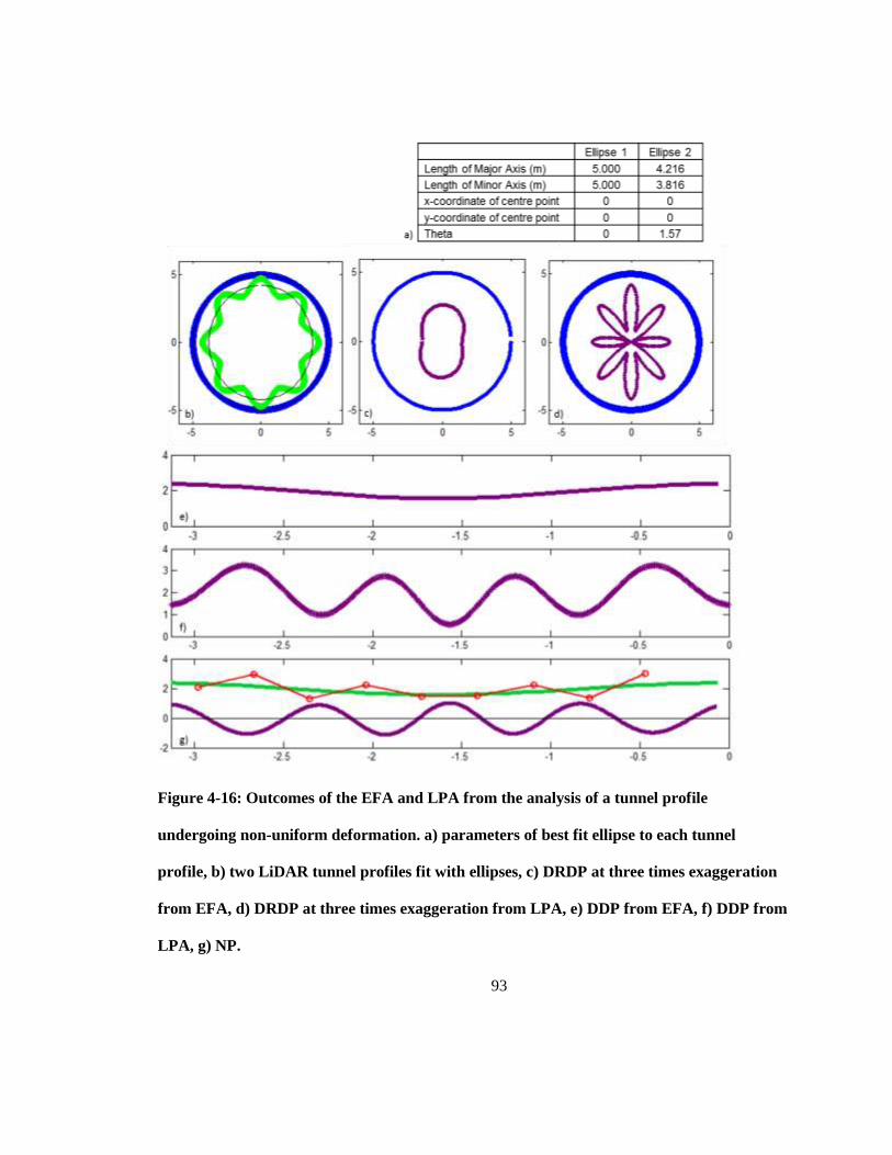
93
Figure 4-16: Outcomes of the EFA and LPA from the analysis of a tunnel profile
undergoing non-uniform deformation. a) parameters of best fit ellipse to each tunnel
profile, b) two LiDAR tunnel profiles fit with ellipses, c) DRDP at three times exaggeration
from EFA, d) DRDP at three times exaggeration from LPA, e) DDP from EFA, f) DDP from
LPA, g) NP.
94
Table 4-1: Parameters varied for sensitivity testing of the EFA and LPA analysis
Parameter Range of values tested Step
β 0 – 0.6 m 0.001 m
ϒ 0 – 30 2
Random noise 0 – 0.5 m 0.001 m
Radius 4.9 – 5.0 m 0.0005 m
Occlusion 0 – 100% 2%
Skew 0 – 0.5 m 0.001 m
For tests with constant system noise, a equal to 0.05 was chosen and a of 6. For
constant change in tunnel size, a radius of 4.95 m was used. Seven tests for each combination of
parameters were completed, and the mean and standard deviation of these seven tests were used
for analysis.
For every test, the first set of data (reference profile) used in the comparison was a
perfectly circular profile with a radius of 5 m. No random or systematic noise, occlusion, or skew
was included in the reference profile. In each of the compared profiles one or more of the
parameters show in Table 4-1 were varied to test the impact on the measurement of convergence
of the tunnel profile. Parameters were tested individually and together to determine if any
combination of parameters had a greater impact on error than each parameter tested alone.
The results of the parametric study were analyzed by looking at the “maximum change
error” ( ) the “minimum change error” ( ) and the “average change error” ( ),
collectively known as the “change errors” or s.
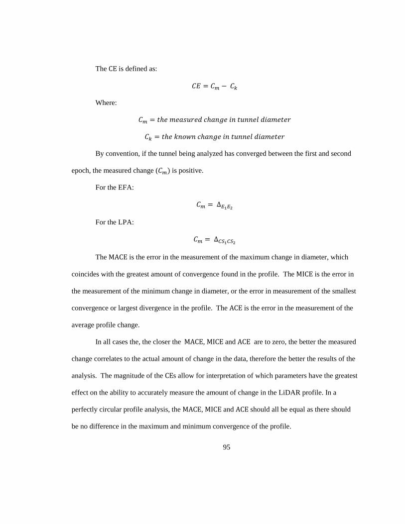
95
The is defined as:
Where:
By convention, if the tunnel being analyzed has converged between the first and second
epoch, the measured change ( ) is positive.
For the EFA:
For the LPA:
The is the error in the measurement of the maximum change in diameter, which
coincides with the greatest amount of convergence found in the profile. The is the error in
the measurement of the minimum change in diameter, or the error in measurement of the smallest
convergence or largest divergence in the profile. The is the error in the measurement of the
average profile change.
In all cases the, the closer the , and are to zero, the better the measured
change correlates to the actual amount of change in the data, therefore the better the results of the
analysis. The magnitude of the s allow for interpretation of which parameters have the greatest
effect on the ability to accurately measure the amount of change in the LiDAR profile. In a
perfectly circular profile analysis, the , and should all be equal as there should
be no difference in the maximum and minimum convergence of the profile.

96
It must be noted that average change error is only an appropriate metric for analysis when
looking at circular deformation of the tunnel profile. When skew is introduced into the
parametric study, only the and can be used for analysis. The standard deviation of
each analysis was also determined.
4.9.1 Results of sensitivity testing with synthetic LiDAR data
Overall the results of the parametric study show that the EFA produces measurements of
convergence that are well below the noise level of the data, and therefore the EFA is a beneficial
methodology for the measurement of convergence. As expected, the LPA analysis produces a
high amount of error in the measurement of minimum and maximum convergence, and is only
useful if the measurement of average convergence is desired.
The results of the parametric study also show that each of the varied parameters is
linearly independent in their effect on the amount of error they cause in the measurement of
convergence.
For both the EFA and LPA, variation of the diameter had no effect on any of the CEs.
The number of systematic deviations of the tunnel profile (gamma) and skew also had no effect
on the CEs of the EFA and LPA. It must be noted that the results for a gamma value less than 4
must be discounted from the analysis, as this does not produce logical or possible tunnel profiles.
The variation of β had a large impact on the MACE and MICE produced by the LPA,
resulting in errors of up to 10 cm in the measurement of diametric convergence. An increased β
also had an impact on the MACE and MICE of the EFA, but the impact was much smaller. At a
maximum systematic deviation of 6 cm the greatest CE was about 0.03 cm (Figure 4-17).
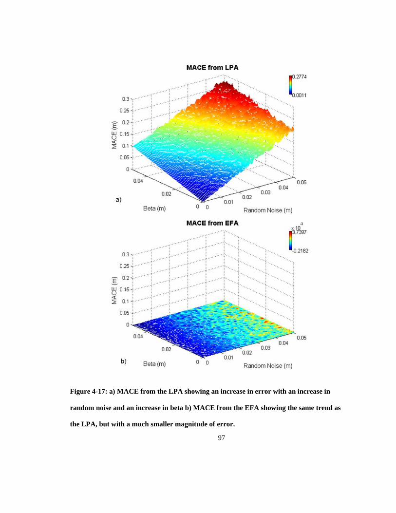
97
Figure 4-17: a) MACE from the LPA showing an increase in error with an increase in
random noise and an increase in beta b) MACE from the EFA showing the same trend as
the LPA, but with a much smaller magnitude of error.
98
The inclusion of random noise in the analysis again impacts both the EFA and LPA, but
the LPA CEs are much greater than those of the EFA. When random noise is included with a
standard deviation of 5 cm, the resulting error in the measurement of convergence by the LPA is
about 23 cm, whereas for the EFA it is about 5 mm. As the measurement of convergence is an
order of magnitude less than the noise included, this proves that the EFA produces accurate
measurements of convergence even when the collected data is noisy.
When both random and systematic noise are included in the data, the impact on the CEs
measured by the LPA and EFA is unchanged. The LPA produced a maximum error of 32 cm at
the highest level of noise, where the EFA produced a maximum error of 4 mm.
From the parametric study it was also determined that a level of up to approximately 60%
occlusion is acceptable for both the EFA and LPA analysis. When the distributed occlusion level
is increased above 60%, the proficiency of both analysis techniques significantly degraded largely
due to the inability to accurately fit an ellipse to the data, and then to position the ellipse or the
raw data for analysis. The results also show that a slightly higher level of occlusion is allowable
for data sets with lower noise levels.
As expected, for analysis of a perfect circle, the magnitude of the MACE and MICE are
very similar. The accuracy of the analysis is further demonstrated by comparing the MACE and
MICE that result from the EFA. When skew is included (Figure 4-18), the MACE and MICE are
very similar, showing that the error in measurement is an absolute error, and not dependent on the
direction or amount of deformation.
99
Figure 4-18: a) MACE from the LPA showing an increase in error with an increase in
random noise and minimal impact of skew on the error b) MACE from the EFA showing
the same trend as the LPA, but with a much smaller magnitude of error.
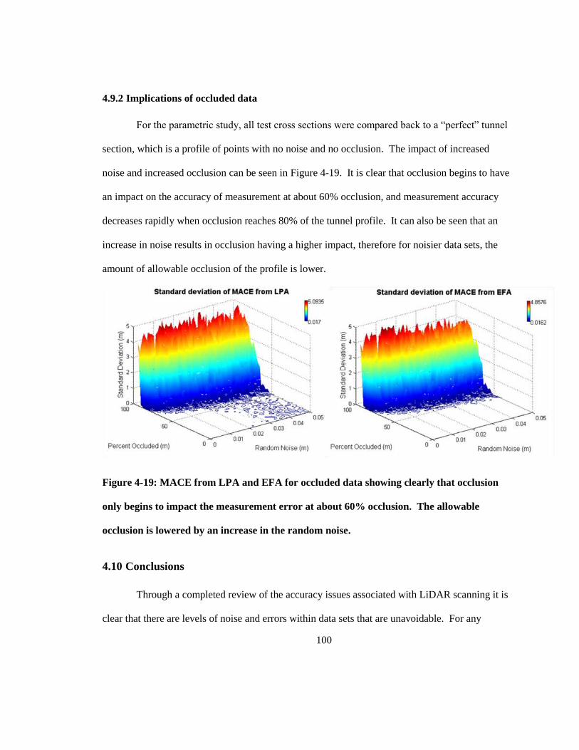
100
4.9.2 Implications of occluded data
For the parametric study, all test cross sections were compared back to a “perfect” tunnel
section, which is a profile of points with no noise and no occlusion. The impact of increased
noise and increased occlusion can be seen in Figure 4-19. It is clear that occlusion begins to have
an impact on the accuracy of measurement at about 60% occlusion, and measurement accuracy
decreases rapidly when occlusion reaches 80% of the tunnel profile. It can also be seen that an
increase in noise results in occlusion having a higher impact, therefore for noisier data sets, the
amount of allowable occlusion of the profile is lower.
Figure 4-19: MACE from LPA and EFA for occluded data showing clearly that occlusion
only begins to impact the measurement error at about 60% occlusion. The allowable
occlusion is lowered by an increase in the random noise.
4.10 Conclusions
Through a completed review of the accuracy issues associated with LiDAR scanning it is
clear that there are levels of noise and errors within data sets that are unavoidable. For any

101
change detection analysis to be useful, it must be able to filter these errors and in some way deal
with noise so that accurate levels of change can be measured. Previous analysis has shown that in
tunnels and shafts, levels of change on the orders of millimeters must be measured. As the
accuracy of single points in LiDAR data is of the same magnitude of this necessary level of
change detection, statistical analysis techniques of profile data are needed. One such technique is
the Elliptical Fit Analysis (EFA) and LiDAR Profile Analysis (LPA) developed by Delaloye et al.
(2012). To ensure that this technique is robust enough to deal with random noise, systematic
noise, and other errors unavoidable during LiDAR scanning, a sensitivity analysis was completed.
The results of the sensitivity analysis show that the combined EFA and LPA analysis can
accurately measure levels of change within the level of raw accuracy of the LiDAR point cloud.
The combined EFA and LPA also have the added benefit that they are able to deal with large
amount of occlusion of the tunnel profile within the data sets. The analysis has shown the level
of error in change detection does not become significant until the occlusion exceeds about 60% of
the tunnel profile. Future analysis should be completed to test the EFA and LPA on real data sets,
and compare the results of LiDAR monitoring results with traditional deformation analysis
techniques.
102
Chapter 5
A New Workflow for LiDAR Scanning for Change Detection in Tunnels
and Caverns3
5.1 Abstract
Measuring change in underground environments is an important aspect of geological
engineering. Recently, methods for using Light Detection and Ranging (LiDAR) to measure
change and convergence in tunnels and other underground environments have been demonstrated.
To properly apply these new methods, it is important that an appropriate workflow is followed.
The workflow proposed in this paper includes recommendations for choosing scan resolution
settings and scan locations based on the level of change to be measured. The workflow follows
through to the extraction of cross-section data for convergence measurement and back
calculation.
5.2 Introduction
The benefit of using Light Detection and Ranging (LiDAR) for geological engineering
applications has been widely demonstrated and discussed in the literature over the past ten years.
3 This chapter appears as submitted to a conference proceedings with the following citation:
Delaloye, D., Hutchinson, J., Diederichs, M. (2012) A New Workflow for LiDAR Scanning for
Change Detection in Tunnels and Caverns. 46th U.S. Rock Mechanics Geomechanics Symposium
ARMA 2012. Chicago, United States.
103
For example, LiDAR can be used for rockmass characterization, discontinuity measurement, and
change detection in underground spaces (Fekete, 2010; Lato, 2010). As the number of
applications of LiDAR scanning is increasing and its use is becoming more commonplace, it is
important to establish best practices for both data collection and data management. More recently
it has been shown that LiDAR data can be used for monitoring tunnel deformations and for
change detection (Delaloye et al., 2012). To ensure that the LiDAR data collected from within
tunnels is of high enough quality for all of these applications, it is important that the appropriate
amount of data is collected from the right locations at the correct resolution.
Previous workflows have been suggested for different geological engineering
applications of LiDAR scanning. Buckley et al. (2008) created a practical workflow for scanning
of large outcrops with long range time of flight laser scanners. The workflow proposed by
Buckley et al. (2008) is very efficient for large scale feature extraction, but must be refined for
application in underground environments, especially if scans are to be used for change detection.
A workflow for discontinuity extraction from underground LiDAR scans for input into stability
models was created by Fekete et al. (2010). Although this workflow is practical for collection of
scans for rockmass characterization, it does not have all the necessary considerations for scanning
for change detection and convergence measurement.
When completing multi-temporal LiDAR scans for change detection, more care has to be
taken in the data acquisition than when only one scan set is collected. This paper will suggest a
new workflow that can be used to ensure that the resolution, accuracy and coverage of LiDAR
scans collected within a tunnel or other underground environment meet data requirements for all
underground scanning applications, with special focus on scanning for change detection. The
workflow focuses on the resolution settings and scan locations needed for optimal and complete
104
coverage of an underground area. Comments are also made on the accuracy issues associated
with LiDAR scanning and how to minimize any manageable errors in the field during data
collection.
Once LiDAR data sets are collected, it is important to use a proper workflow for data
management and analysis. In addition to recommendations for data collection, this paper extends
the workflow to include suggestions for managing multiple data sets and how they can be
analyzed for the aforementioned underground applications. Implications of processing
techniques on data accuracy and measurement resolution are also included in the workflow.
5.3 LiDAR scanning for deformation measurement
The applications of LiDAR scanning in underground excavations are continually
growing. LiDAR has been demonstrated to be useful for discontinuity orientation measurement,
rockmass characterization, and as built modeling Fekete et al. (2010). A summary of some of the
main applications of LiDAR in tunneling environments to date is shown in Figure 5-1. One of
the most recent LiDAR scanning applications is for the measurement of deformation in tunnels
(Delaloye et al. 2012, van Gosliga et al., (2006), Lindenberg et al. (2009)). Before using LiDAR
for tunnel deformation measurement, it is important to discuss the sources of error, as the level of
accuracy and noise in the data has implications as to the level of convergence that can be
measured in the tunnel or cavern.
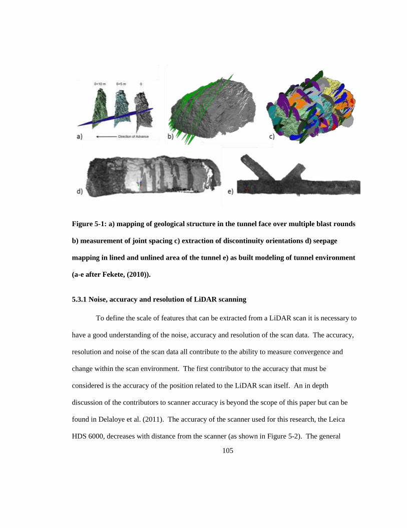
105
Figure 5-1: a) mapping of geological structure in the tunnel face over multiple blast rounds
b) measurement of joint spacing c) extraction of discontinuity orientations d) seepage
mapping in lined and unlined area of the tunnel e) as built modeling of tunnel environment
(a-e after Fekete, (2010)).
5.3.1 Noise, accuracy and resolution of LiDAR scanning
To define the scale of features that can be extracted from a LiDAR scan it is necessary to
have a good understanding of the noise, accuracy and resolution of the scan data. The accuracy,
resolution and noise of the scan data all contribute to the ability to measure convergence and
change within the scan environment. The first contributor to the accuracy that must be
considered is the accuracy of the position related to the LiDAR scan itself. An in depth
discussion of the contributors to scanner accuracy is beyond the scope of this paper but can be
found in Delaloye et al. (2011). The accuracy of the scanner used for this research, the Leica
HDS 6000, decreases with distance from the scanner (as shown in Figure 5-2). The general
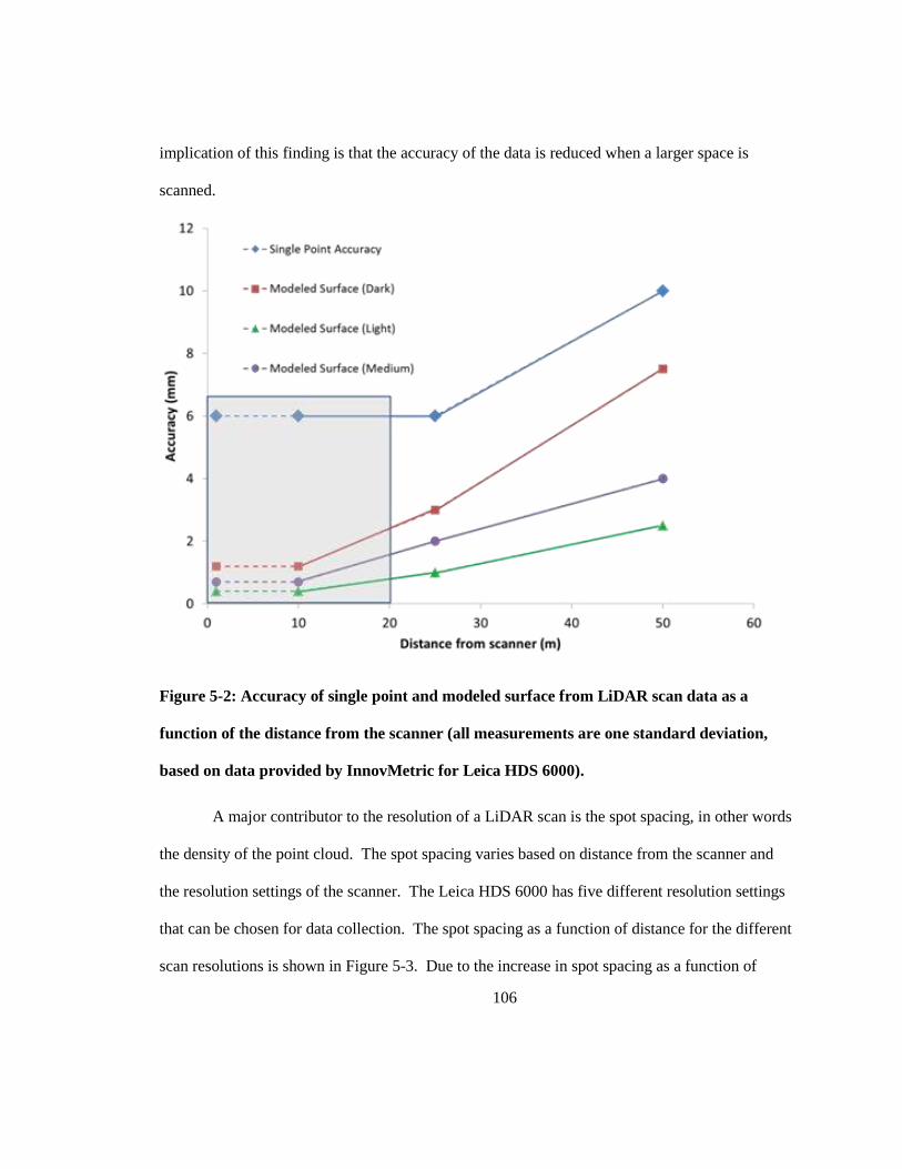
106
implication of this finding is that the accuracy of the data is reduced when a larger space is
scanned.
Figure 5-2: Accuracy of single point and modeled surface from LiDAR scan data as a
function of the distance from the scanner (all measurements are one standard deviation,
based on data provided by InnovMetric for Leica HDS 6000).
A major contributor to the resolution of a LiDAR scan is the spot spacing, in other words
the density of the point cloud. The spot spacing varies based on distance from the scanner and
the resolution settings of the scanner. The Leica HDS 6000 has five different resolution settings
that can be chosen for data collection. The spot spacing as a function of distance for the different
scan resolutions is shown in Figure 5-3. Due to the increase in spot spacing as a function of
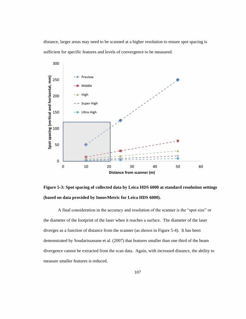
107
distance, larger areas may need to be scanned at a higher resolution to ensure spot spacing is
sufficient for specific features and levels of convergence to be measured.
Figure 5-3: Spot spacing of collected data by Leica HDS 6000 at standard resolution settings
(based on data provided by InnovMetric for Leica HDS 6000).
A final consideration in the accuracy and resolution of the scanner is the “spot size” or
the diameter of the footprint of the laser when it reaches a surface. The diameter of the laser
diverges as a function of distance from the scanner (as shown in Figure 5-4). It has been
demonstrated by Soudarissanane et al. (2007) that features smaller than one third of the beam
divergence cannot be extracted from the scan data. Again, with increased distance, the ability to
measure smaller features is reduced.
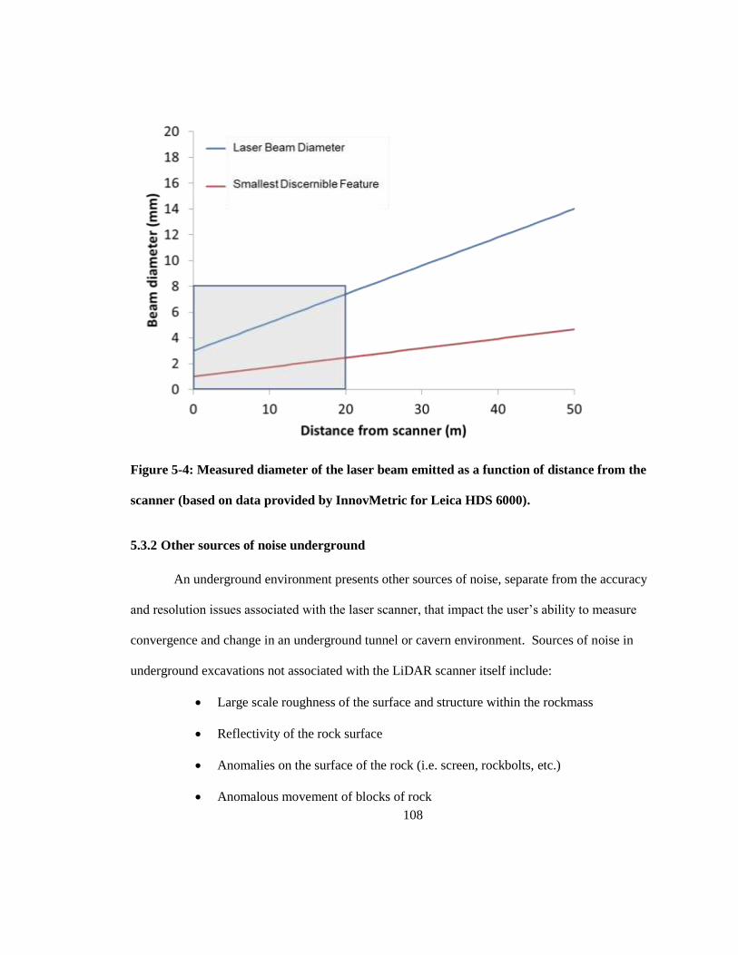
108
Figure 5-4: Measured diameter of the laser beam emitted as a function of distance from the
scanner (based on data provided by InnovMetric for Leica HDS 6000).
5.3.2 Other sources of noise underground
An underground environment presents other sources of noise, separate from the accuracy
and resolution issues associated with the laser scanner, that impact the user’s ability to measure
convergence and change in an underground tunnel or cavern environment. Sources of noise in
underground excavations not associated with the LiDAR scanner itself include:
Large scale roughness of the surface and structure within the rockmass
Reflectivity of the rock surface
Anomalies on the surface of the rock (i.e. screen, rockbolts, etc.)
Anomalous movement of blocks of rock
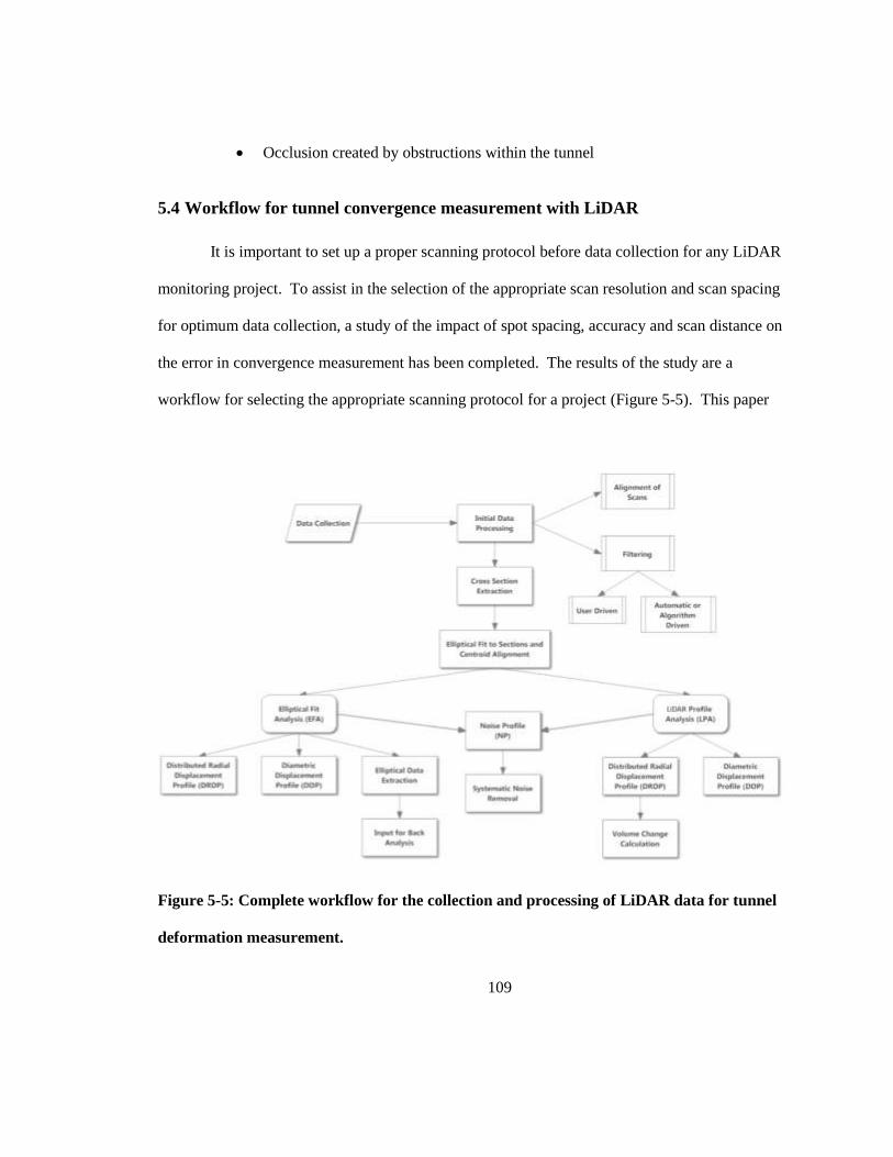
109
Occlusion created by obstructions within the tunnel
5.4 Workflow for tunnel convergence measurement with LiDAR
It is important to set up a proper scanning protocol before data collection for any LiDAR
monitoring project. To assist in the selection of the appropriate scan resolution and scan spacing
for optimum data collection, a study of the impact of spot spacing, accuracy and scan distance on
the error in convergence measurement has been completed. The results of the study are a
workflow for selecting the appropriate scanning protocol for a project (Figure 5-5). This paper
Figure 5-5: Complete workflow for the collection and processing of LiDAR data for tunnel
deformation measurement.
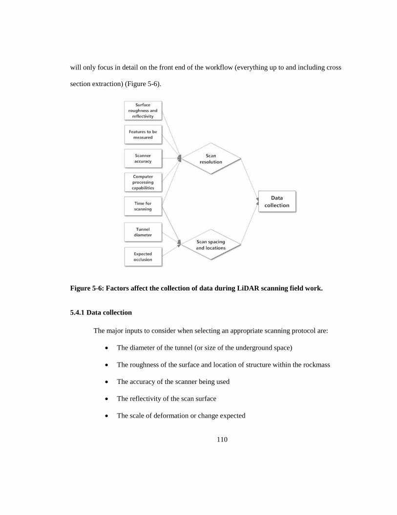
110
will only focus in detail on the front end of the workflow (everything up to and including cross
section extraction) (Figure 5-6).
Figure 5-6: Factors affect the collection of data during LiDAR scanning field work.
5.4.1 Data collection
The major inputs to consider when selecting an appropriate scanning protocol are:
The diameter of the tunnel (or size of the underground space)
The roughness of the surface and location of structure within the rockmass
The accuracy of the scanner being used
The reflectivity of the scan surface
The scale of deformation or change expected
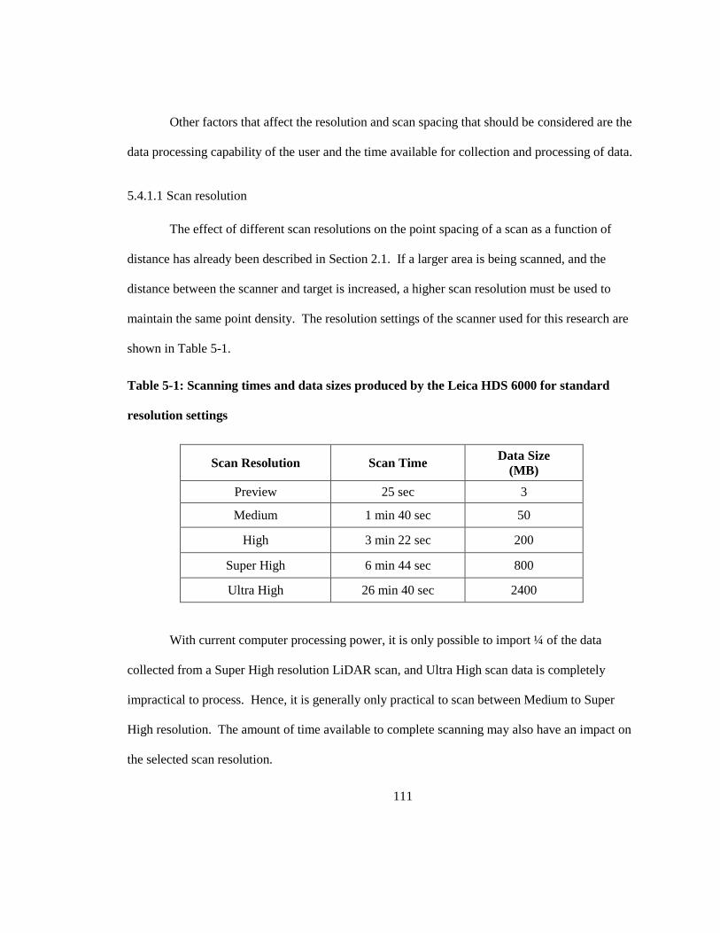
111
Other factors that affect the resolution and scan spacing that should be considered are the
data processing capability of the user and the time available for collection and processing of data.
5.4.1.1 Scan resolution
The effect of different scan resolutions on the point spacing of a scan as a function of
distance has already been described in Section 2.1. If a larger area is being scanned, and the
distance between the scanner and target is increased, a higher scan resolution must be used to
maintain the same point density. The resolution settings of the scanner used for this research are
shown in Table 5-1.
Table 5-1: Scanning times and data sizes produced by the Leica HDS 6000 for standard
resolution settings
Scan Resolution Scan Time Data Size
(MB)
Preview 25 sec 3
Medium 1 min 40 sec 50
High 3 min 22 sec 200
Super High 6 min 44 sec 800
Ultra High 26 min 40 sec 2400
With current computer processing power, it is only possible to import ¼ of the data
collected from a Super High resolution LiDAR scan, and Ultra High scan data is completely
impractical to process. Hence, it is generally only practical to scan between Medium to Super
High resolution. The amount of time available to complete scanning may also have an impact on
the selected scan resolution.
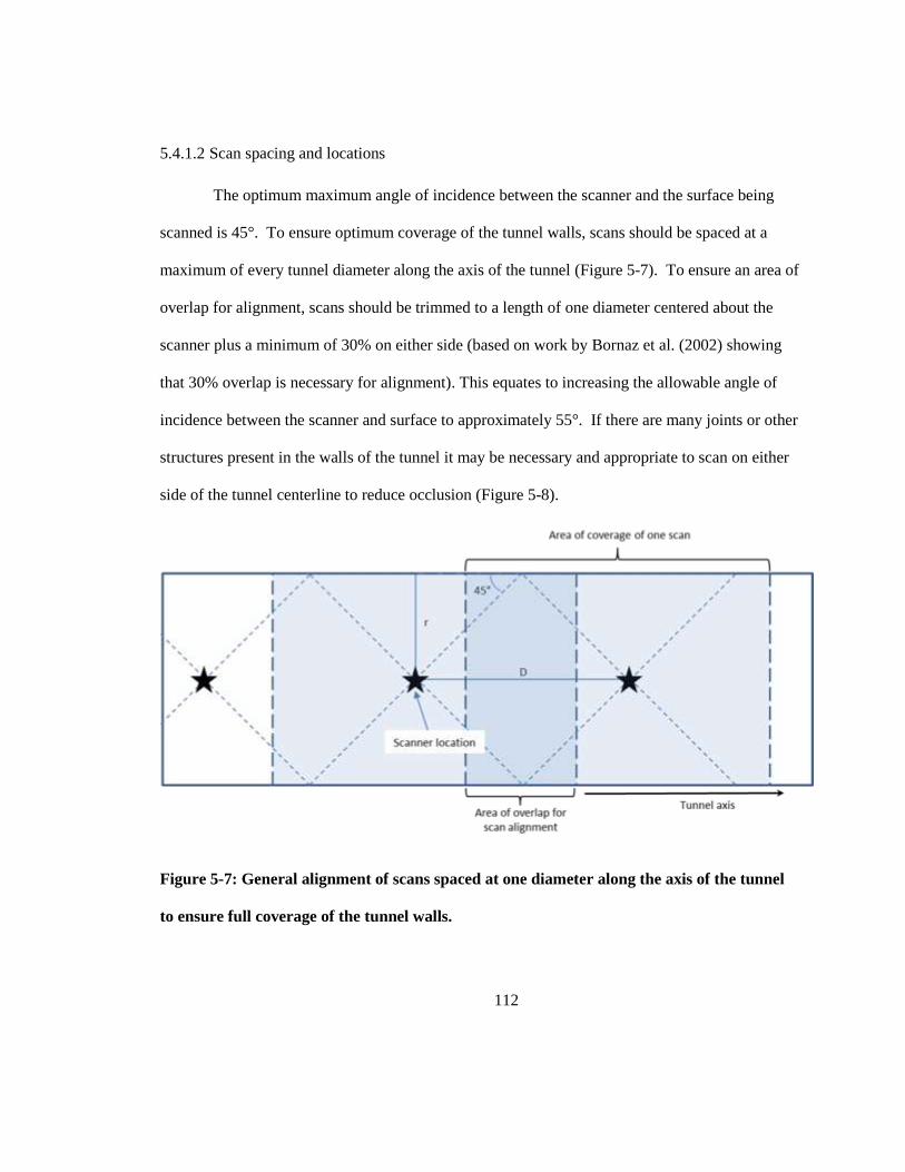
112
5.4.1.2 Scan spacing and locations
The optimum maximum angle of incidence between the scanner and the surface being
scanned is 45°. To ensure optimum coverage of the tunnel walls, scans should be spaced at a
maximum of every tunnel diameter along the axis of the tunnel (Figure 5-7). To ensure an area of
overlap for alignment, scans should be trimmed to a length of one diameter centered about the
scanner plus a minimum of 30% on either side (based on work by Bornaz et al. (2002) showing
that 30% overlap is necessary for alignment). This equates to increasing the allowable angle of
incidence between the scanner and surface to approximately 55°. If there are many joints or other
structures present in the walls of the tunnel it may be necessary and appropriate to scan on either
side of the tunnel centerline to reduce occlusion (Figure 5-8).
Figure 5-7: General alignment of scans spaced at one diameter along the axis of the tunnel
to ensure full coverage of the tunnel walls.
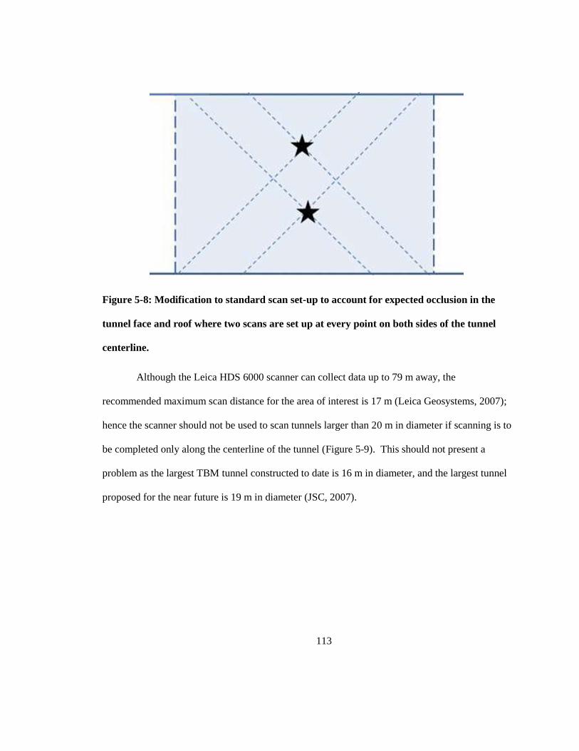
113
Figure 5-8: Modification to standard scan set-up to account for expected occlusion in the
tunnel face and roof where two scans are set up at every point on both sides of the tunnel
centerline.
Although the Leica HDS 6000 scanner can collect data up to 79 m away, the
recommended maximum scan distance for the area of interest is 17 m (Leica Geosystems, 2007);
hence the scanner should not be used to scan tunnels larger than 20 m in diameter if scanning is to
be completed only along the centerline of the tunnel (Figure 5-9). This should not present a
problem as the largest TBM tunnel constructed to date is 16 m in diameter, and the largest tunnel
proposed for the near future is 19 m in diameter (JSC, 2007).
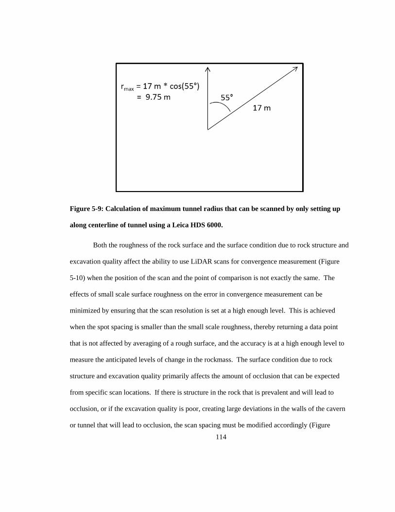
114
Figure 5-9: Calculation of maximum tunnel radius that can be scanned by only setting up
along centerline of tunnel using a Leica HDS 6000.
Both the roughness of the rock surface and the surface condition due to rock structure and
excavation quality affect the ability to use LiDAR scans for convergence measurement (Figure
5-10) when the position of the scan and the point of comparison is not exactly the same. The
effects of small scale surface roughness on the error in convergence measurement can be
minimized by ensuring that the scan resolution is set at a high enough level. This is achieved
when the spot spacing is smaller than the small scale roughness, thereby returning a data point
that is not affected by averaging of a rough surface, and the accuracy is at a high enough level to
measure the anticipated levels of change in the rockmass. The surface condition due to rock
structure and excavation quality primarily affects the amount of occlusion that can be expected
from specific scan locations. If there is structure in the rock that is prevalent and will lead to
occlusion, or if the excavation quality is poor, creating large deviations in the walls of the cavern
or tunnel that will lead to occlusion, the scan spacing must be modified accordingly (Figure
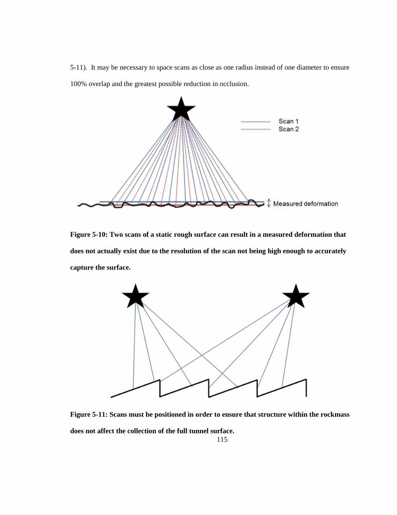
115
5-11). It may be necessary to space scans as close as one radius instead of one diameter to ensure
100% overlap and the greatest possible reduction in occlusion.
Figure 5-10: Two scans of a static rough surface can result in a measured deformation that
does not actually exist due to the resolution of the scan not being high enough to accurately
capture the surface.
Figure 5-11: Scans must be positioned in order to ensure that structure within the rockmass
does not affect the collection of the full tunnel surface.
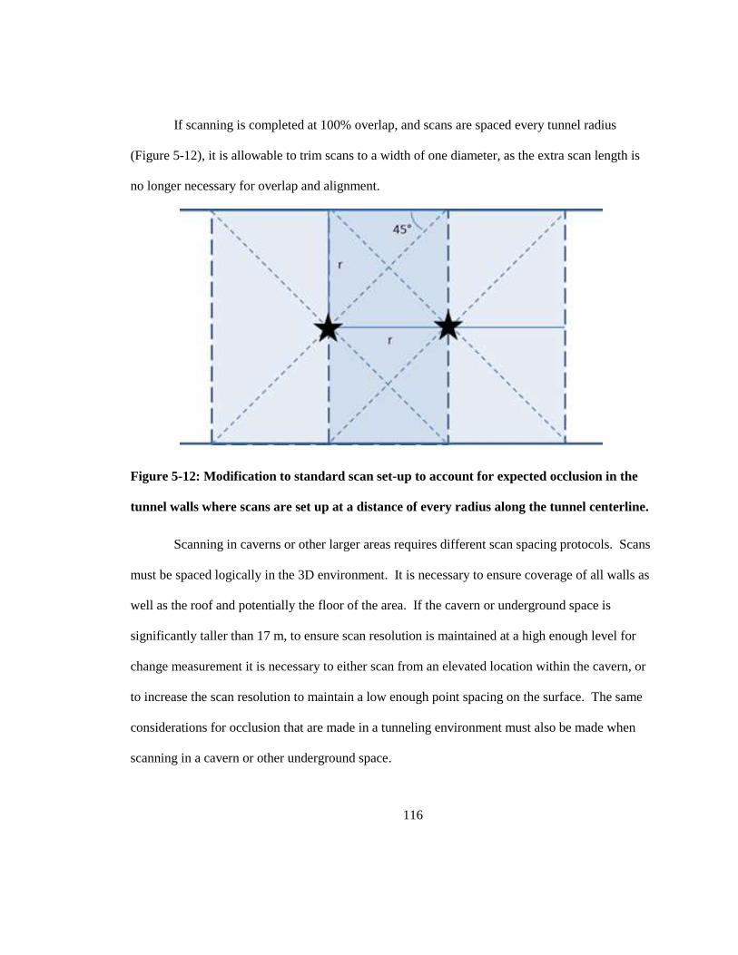
116
If scanning is completed at 100% overlap, and scans are spaced every tunnel radius
(Figure 5-12), it is allowable to trim scans to a width of one diameter, as the extra scan length is
no longer necessary for overlap and alignment.
Figure 5-12: Modification to standard scan set-up to account for expected occlusion in the
tunnel walls where scans are set up at a distance of every radius along the tunnel centerline.
Scanning in caverns or other larger areas requires different scan spacing protocols. Scans
must be spaced logically in the 3D environment. It is necessary to ensure coverage of all walls as
well as the roof and potentially the floor of the area. If the cavern or underground space is
significantly taller than 17 m, to ensure scan resolution is maintained at a high enough level for
change measurement it is necessary to either scan from an elevated location within the cavern, or
to increase the scan resolution to maintain a low enough point spacing on the surface. The same
considerations for occlusion that are made in a tunneling environment must also be made when
scanning in a cavern or other underground space.
117
5.4.2 Initial data processing
Once data is collected, it is important that the proper processing workflow be followed to
ensure feature extraction and convergence measurement can be completed. The first steps in data
processing are loading the scans, and trimming them to the area of interest. For tunneling it is
suggested that scans be trimmed to one diameter plus 30% on either side of the scan to allow
overlap for alignment.
5.4.2.1 Alignment of scans
An area of overlap between two scans must be used for alignment. The alignment can be
done by matching targets captured in both scans, using objects within the scan as reference points
for alignment or by using a computer driven algorithm alignment. The most common computer
driven alignment is the Iterative Closest Point (ICP) algorithm. It was developed for the
alignment of point clouds by Besl & McKay (1992) and is a data driven registration method.
This is a widely used algorithm, and is the built in registration method for most software
programs, including PolyWorks® V 11.0.28 (InnovMetric (2011). For alignment in true space,
targets within the scan environment can be located using georeferencing.
5.4.2.2 Filtering of data
Initial data processing also includes the filtering of data. Filtering can be either user
driven, or be completed using a filtering algorithm. User driven filtering can be done to remove
large anomalies in the scan, such as pieces of equipment or machinery. It is not practical to use
user driven filtration to remove smaller and near surface anomalies as it is too time consuming.
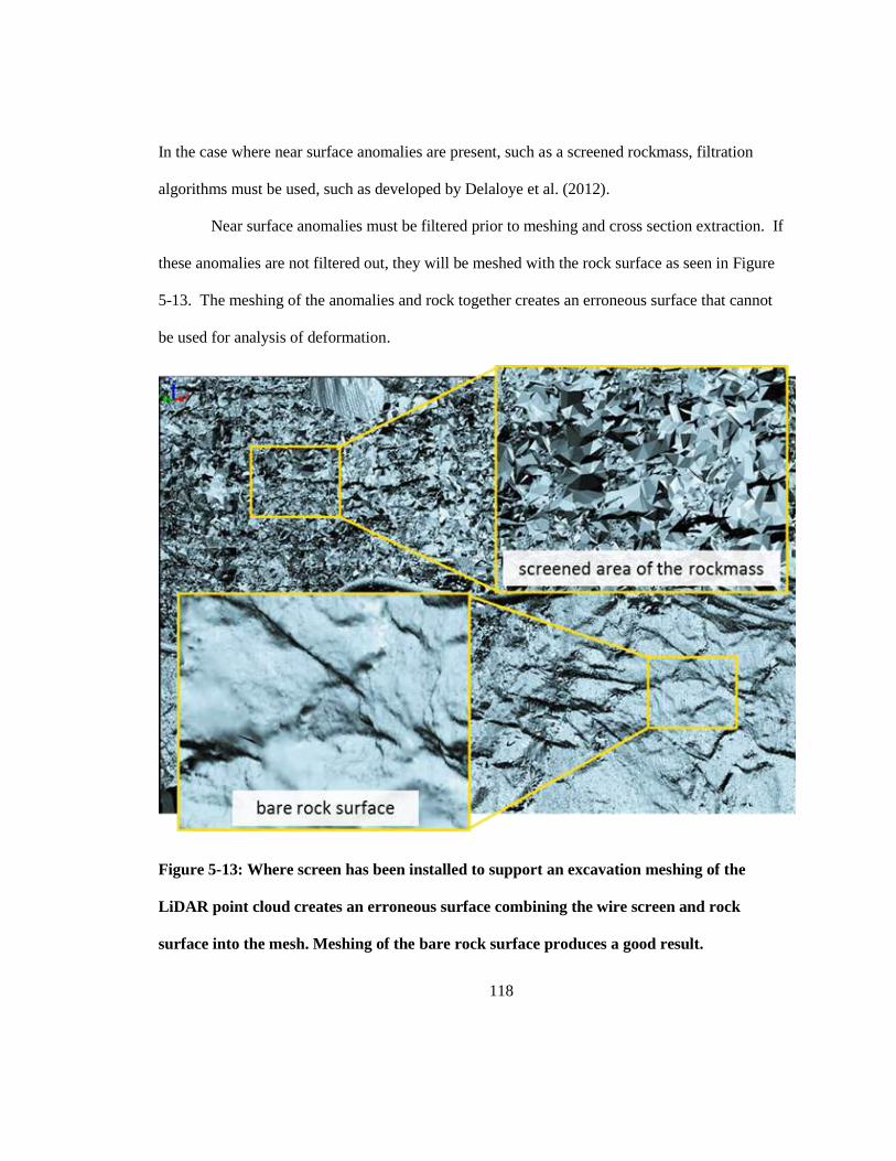
118
In the case where near surface anomalies are present, such as a screened rockmass, filtration
algorithms must be used, such as developed by Delaloye et al. (2012).
Near surface anomalies must be filtered prior to meshing and cross section extraction. If
these anomalies are not filtered out, they will be meshed with the rock surface as seen in Figure
5-13. The meshing of the anomalies and rock together creates an erroneous surface that cannot
be used for analysis of deformation.
Figure 5-13: Where screen has been installed to support an excavation meshing of the
LiDAR point cloud creates an erroneous surface combining the wire screen and rock
surface into the mesh. Meshing of the bare rock surface produces a good result.
119
Once the scan data has been properly filtered, the point cloud can be turned into a surface
model for the extraction of cross sections.
5.4.3 Cross section extraction
There are two different possible methods of cross section extraction. If a surface has
been modeled from the point cloud, a cross section of that surface should be extracted for
convergence measurement. Care should be taken to ensure cross sections taken from multi-
temporal scans are extracted in the same (or as near as possible) location.
If the LiDAR data is not turned into a meshed surface it is still possible to use the raw
point cloud for cross section extraction. In this case a narrow swath of data should be used for
comparison. The use of a swath of data reduces the accuracy needed in the selection of the same
cross section of data by allowing for averaging over a small area to be completed. Another
benefit of using a swath of data is that the swath allows for some of the noise and roughness
within the scan to be averaged out, as the points are just treated as one cross section throughout
the rest of the analysis. It must be ensured that the section is taken perpendicular to the axis of
the tunnel within +/- 1° to ensure that no skew in the profile is introduced.
5.5 Convergence measurement
To measure convergence within a tunnel, the Elliptical Fitting Analysis (EFA) and
LiDAR Profile Analysis (LPA) was proposed by Delaloye et al., (2012). The analysis requires
two tunnel profiles extracted from LiDAR data (or other point cloud data) as input. The
robustness of the EFA and LPA analysis has previously been demonstrated, but the required
resolution for extraction of specific measurements of convergence, and at different tunneling
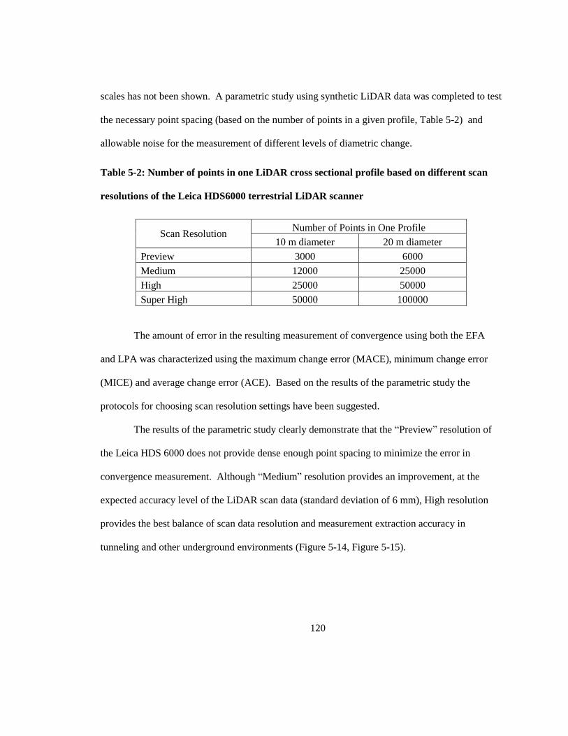
120
scales has not been shown. A parametric study using synthetic LiDAR data was completed to test
the necessary point spacing (based on the number of points in a given profile, Table 5-2) and
allowable noise for the measurement of different levels of diametric change.
Table 5-2: Number of points in one LiDAR cross sectional profile based on different scan
resolutions of the Leica HDS6000 terrestrial LiDAR scanner
Scan Resolution Number of Points in One Profile
10 m diameter 20 m diameter
Preview 3000 6000
Medium 12000 25000
High 25000 50000
Super High 50000 100000
The amount of error in the resulting measurement of convergence using both the EFA
and LPA was characterized using the maximum change error (MACE), minimum change error
(MICE) and average change error (ACE). Based on the results of the parametric study the
protocols for choosing scan resolution settings have been suggested.
The results of the parametric study clearly demonstrate that the “Preview” resolution of
the Leica HDS 6000 does not provide dense enough point spacing to minimize the error in
convergence measurement. Although “Medium” resolution provides an improvement, at the
expected accuracy level of the LiDAR scan data (standard deviation of 6 mm), High resolution
provides the best balance of scan data resolution and measurement extraction accuracy in
tunneling and other underground environments (Figure 5-14, Figure 5-15).
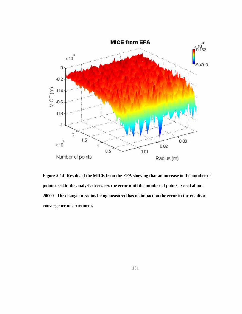
121
Figure 5-14: Results of the MICE from the EFA showing that an increase in the number of
points used in the analysis decreases the error until the number of points exceed about
20000. The change in radius being measured has no impact on the error in the results of
convergence measurement.
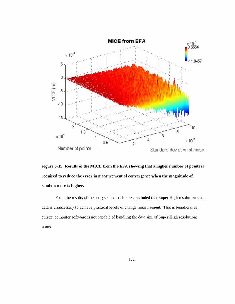
122
Figure 5-15: Results of the MICE from the EFA showing that a higher number of points is
required to reduce the error in measurement of convergence when the magnitude of
random noise is higher.
From the results of the analysis it can also be concluded that Super High resolution scan
data is unnecessary to achieve practical levels of change measurement. This is beneficial as
current computer software is not capable of handling the data size of Super High resolutions
scans.
123
5.6 Conclusions
LiDAR is becoming an increasingly common tool for use in geological engineering due
to its ability to rapidly acquire large, high accuracy, high precision positional data sets. To ensure
the correct resolution and coverage of LiDAR scans are collected during a field program, it is
important to develop and implement comprehensive workflows. The workflow created in this
paper suggests techniques for selecting the appropriate locations and scan resolutions for data
collected in tunnels and other underground environments to be later used for change detection and
convergence measurement. In general scans should be spaced at a maximum of every diameter
down the axis of the tunnel, and scan resolution should be set at “High” (for the Leica HDS 6000)
or a similar setting such that the number of points on the profile is at least 20000.
124
Chapter 6
General discussion
6.1 Discussion
Two different profile analysis techniques have been developed in this thesis to take
advantage of the different opportunities that each approach provides. The Elliptical Fit Analysis
(EFA) analysis is to be used for extracting accurate information about the overall deformation of
the tunnel, and can provide data that can be used for back analysis. The LiDAR Profile Analysis
(LPA) is used for identification of local anomalous movements that deviate from the overall
deformation profile trend.
6.2 Limitations
The current profile analysis code is limited to the analysis of circular and near circular
tunnels and shafts. Mean deformation ellipse analysis is not considered to be practical at this
point for other shape of excavations, as the author has developed the analysis specifically for
diametric deformation and closure measurement. The code can be refined in the future to allow
for application to other shapes of excavations such as horseshoe tunnels and square caverns.
The developed algorithm is limited in that it can only measure tunnel or shaft
convergence, and cannot account for vertical or lateral shift. Although this is a limitation of the
current analysis, it is rarely necessary to account for lateral or vertical movement for a single
tunnel analysis; convergence is by far the most important component of tunnel displacement
measurement. If the user does desire to measure vertical and lateral movement it is possible to
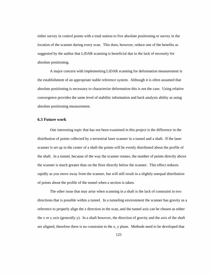
125
either survey in control points with a total station to five absolute positioning or survey in the
location of the scanner during every scan. This does, however, reduce one of the benefits as
suggested by the author that LiDAR scanning is beneficial due to the lack of necessity for
absolute positioning.
A major concern with implementing LiDAR scanning for deformation measurement is
the establishment of an appropriate stable reference system. Although it is often assumed that
absolute positioning is necessary to characterize deformation this is not the case. Using relative
convergence provides the same level of stability information and back analysis ability as using
absolute positioning measurement.
6.3 Future work
One interesting topic that has not been examined in this project is the difference in the
distribution of points collected by a terrestrial laser scanner in a tunnel and a shaft. If the laser
scanner is set up in the center of a shaft the points will be evenly distributed about the profile of
the shaft. In a tunnel, because of the way the scanner rotates, the number of points directly above
the scanner is much greater than on the floor directly below the scanner. This effect reduces
rapidly as you move away from the scanner, but will still result in a slightly unequal distribution
of points about the profile of the tunnel when a section is taken.
The other issue that may arise when scanning in a shaft is the lack of constraint in two
directions that is possible within a tunnel. In a tunneling environment the scanner has gravity as a
reference to properly align the z direction in the scan, and the tunnel axis can be chosen as either
the x or y axis (generally y). In a shaft however, the direction of gravity and the axis of the shaft
are aligned, therefore there is no constraint in the x, y plane. Methods need to be developed that
126
will allow for the direction in the x, y plane to be constrained. This could be as simple as
ensuring there is paint on the wall of the shaft located in the direction of the chosen z axis.
In future, it is suggested that Fourier analysis be incorporated into the analysis of the
LiDAR profiles to assist in the removal of systematic noise from the data. Fourier analysis is
commonly used in signal processing to remove background noise from data using the frequency
spectrum. By removing background noise from LiDAR profiles, trends in deformation data will
be easier to extract and use for back analysis.
The developed code is not limited to profile analysis of tunnels derived from LiDAR
data. The code is robust enough to handle any point cloud data, and can be applied to any scale
of measurement. As such, the code would be very valuable in its application to measuring
deformation for boreholes collected with sonic logging. The code has the ability to show the
difference between an ellipse and the actual profile, and therefore could be used to quantify
borehole breakout compared to borehole deformation.
As the code has been developed to handle any general point cloud, it is also not limited to
specifically using LiDAR data. In the future this code can be tested and applied to any point
cloud. It may be useful to use the code to compare the results of LiDAR data collection to
photogrammetry in underground environments.
To more easily deal with data sets with near surface anomalies, full surface filtering
algorithms need to be developed. This thesis has presented a method for filtering sections of data,
and the same logic of using a “look window” and “filter cutoff” could be applied to swaths of
data, and be continued along the entire tunnel profile.
127
Chapter 7
Summary and Conclusions
7.1 Summary
The major advantages of using LiDAR for deformation monitoring that have been
discussed in this thesis are:
1) Acquisition of large sets of high precision, high accuracy positional data is very fast: a
scan can be set up and completed in less than seven minutes
2) Geo-referencing of scans is not required for tunnel convergence measurement: relative
convergence measurements are extremely useful for deformation monitoring and absolute
positioning is not actually necessary.
3) Full surface characterization is possible due to the high point density acquired from
single scan: rather than just monitoring single points, the full surface is characterized.
Top properly apply LiDAR scan data for the measurement of convergence in near
circular tunnels and shafts, a method for profile analysis was created and coded in Matlab. The
combined Elliptical Fit Analysis (EFA) and LiDAR Profile Analysis (EFA) developed in this
thesis allows for complete profile analysis. In addition, the code allows for:
noise to be quantified and areas of anomalous movement to be identified
accurate calculation of volumes of convergence and divergence
both elliptical fit analysis and raw LiDAR profile analysis
Although the EFA and LPA have only been demonstrated using LiDAR point cloud data,
they can easily be used for other data sets such as photogrammetry point cloud data.
128
7.2 Contributions
The research conducted during the preparation of this thesis has been the source for many
publications and presentations. Presented below is a full list of the contributions resulting from
this research.
7.2.1 Refereed Journal Articles (Submitted)
Delaloye, D., Walton, G., Hutchinson, J., Diederichs, M. (2012) Development of an Elliptical
Fitting Algorithm for Tunnel Deformation Monitoring with Static Terrestrial LiDAR
Scanning. Tunneling and Underground Space Technology
Delaloye, D., Hutchinson, J., Diederichs, M. (2012) Sensitivity Testing of the Newly Developed
Elliptical Fitting Method for the Measurement of Convergence in Tunnels and Shafts.
Rock Mechanics and Rock Engineering.
7.2.2 Refereed Conference Papers
Delaloye, D., Hutchinson, J., Diederichs, M. (2012) Application of elliptical fit algorithm for
tunnel deformation monitoring with LiDAR. TAC 2012 Tunnels and Underground
Spaces: Sustainability and Innovations. Montreal, Canada
Delaloye, D., Hutchinson, J., Diederichs, M. (2012) A new workflow for lidar scanning for
change detection in tunnels and caverns. 46th U.S. Rock Mechanics Geomechanics
Symposium ARMA 2012. Chicago, United States
Delaloye, D., Hutchinson, J., Diederichs, M. (2012) Using terrestrial lidar for tunnel deformation
monitoring in circular tunnels and shafts. Eurock 2012. Stockholm, Sweden
129
Valley, B., Milkereit, B., Pun, W., Pilz, M., Hutchinson, J., Delaloye, D., Madjdabadi, B.M.,
Dusseault, M., Thibodeau, D., Forsythe, A. (2012) Rock mass change monitoring in a sill
pillar at Vale’s Coleman mine (Sudbury, Canada). 21st Canadian Rock Mechanics
Symposium RockEng12. Edmonton, Canada
Delaloye, D., Hutchinson, J., Diederichs, M. (2011) Accuracy issues associated with Lidar
scanning for tunnel deformation monitoring. PanAm CGS Geotechnical Conference.
Edmonton, Canada
7.2.3 Non-refereed Conference Presentations
Delaloye, D. (2012) New algorithm for mesh filtration for tunnel profile analysis with LiDAR.
Advances in Earth Science Research Conference. Kingston, Canada
7.2.4 Courses instructed
Short Course Co-Instructor: Lidar Imaging for Mining - Expanding the state-of-practice with
state-of-art tools. At the Centre for Excellence in Mining Innovation (CEMI). October
2011. Sudbury, Ontario, Canada.
7.3 References
Abellan, A., Jaboyedoff, M., Oppikofer, T., Vilaplana, J. M. 2009. Detection of millimetric
deformation using a terrestrial laser scanner: Experiment and application to a rockfall
event. Natural Hazards and Earth System Science, 9(2), 365-372.
Abellan, A., Vilaplana, J. M., Calvet, J., Garcia-Selles, D., Asensio, E. 2011. Rockfall monitoring
by Terrestrial Laser Scanning - Case study of the basaltic rock face at Castellfollit de la
Roca (Catalonia, Spain). Natural Hazards and Earth System Science, 11(3), 829-841.
130
Barla, G., Bonini, M., Debernardi, D. 2008. Time dependent deformations in squeezing tunnels.
In: The 12th International Conference of International Association for Computer Methods
and Advances in Geomechanics, Goa, India.
Besl, P. J., McKay, N. D. 1992. A method for registration of 3-D shapes. IEEE Transactions on
Pattern Analysis and Machine Intelligence, 14(2), 239-256.
Boehler, W., Bordas Vincent, M., Marbs, A. 2003. Investigating laser scanner accuracy. In: The
XIXth CIPA Symposium, Antaylya, Turkey.
Buckley, S. J., Howell, J. A., Enge, H. D., Kurz, T. H. 2008. Terrestrial laser scanning in
geology: Data acquisition, processing and accuracy considerations. Journal of the
Geological Society, 165(3), 625-638.
Burton, D., Dunlap, D. B., Wood, L. J., Flaig, P. P. 2010. Lidar intensity as a remote sensor of
rock properties. Journal of Sedimentary Research, 81(5), 339-347.
Decker, J. B., Dove, J. E. 2008. Laser scanning techniques in Devil's Slide tunnels. In: Laser and
Photogrammetric Methods for Rock Tunnel Characterization Workshop. Tononm F.
(Ed.). 42nd US Rock Mechanics Symposium, San Francisco.
Errington, A. F. C., Daku, B. L. F., Prugger, A. 2010. Closure monitoring in Potash Mines using
LiDAR. In: The IEEE, Piscataway, NJ, USA.
Fekete, S., Diederichs, M., Lato, M. 2010. Geotechnical and operational applications for 3-
dimensional laser scanning in drill and blast tunnels. Tunnelling and Underground Space
Technology, 25(5), 614-628.
Fitzgibbon, A. W., Pilu, M., Fisher, R. B. 1996. Direct least squares fitting of ellipses. In: The
13th International Conference on Pattern Recognition, Los Alamitos, CA, USA.
131
Gigli, G., Casagli, N. 2011. Semi-automatic extraction of rock mass structural data from high
resolution LIDAR point clouds. International Journal of Rock Mechanics and Mining
Sciences, 48(2), 187-198.
Gordon, S. J., Lichti, D. D. 2007. Modelling terrestrial laser scanner data for precise structural
deformation measurement. Journal of Surveying Engineering, 133(2), 72-80.
Hashimoto, T., Koyama, Y., Yingyonggrattanakul, N., Kayukawa, K., Konda, T., Sugimoto, M.
2006. Applications of the new deformation meter for monitoring tunnel lining
deformation. In: The International Symposium on Underground Excavation and
Tunnelling, Bangkok, Thailand.
Hui, H., Fernandez-Steeger, T. M., Mei, D., Hieu Trung, N., Azzam, R. 2010. 3D Modelling
using LiDAR data and its geological and geotechnical applications. In: The 18th
International Conference on Geoinformatics, Piscataway, NJ, USA.
InnovMetric. 2011. PolyWorks V11.0.28. InnovMetric, Quebec.
Ioannidis, C., Valani, A., Georgopolous, A., Tsiligiris, E. 2006. 3D model generation for
deformation analysis using laser scanning data of a cooling tower. In: The 3rd IAG
Symposium on Geodesy for Geotechnical and Structural Engineering and 12th FIG
Symposium on Deformation Measurement, Baden, Austria.
Jaboyedoff, M., Demers, D., Locat, J., Locat, A., Locat, P., Oppikofer, T., Robitaille, D., Turnel,
D. 2009. Use of terrestrial laser scanning for the characterization of retrogressive
landslides in sensitive clay and rotational landslides in river banks. Canadian
Geotechnical Journal, 46(12), 1379-1390.
Jacobs, G. 2006. Understanding spot size for laser scanning. In: Professional Surveyor Magazine,
pp. 1-3.

132
Jacobs, G. 2009. Accuracy of scan points. In: Professional Surveyor Magazine, pp. 1-3.
JSC. 2007. Construction of the Orlovski tunnel under the Neva River in St. Petersburg, Project
Brief, September 2007.
Lato, M., Diederichs, M. S., Hutchinson, D. J., Harrap, R. 2009. Optimization of LiDAR
scanning and processing for automated structural evaluation of discontinuities in
rockmasses. International Journal of Rock Mechanics and Mining Sciences, 46(1), 194-
199.
Leica Geosystems. 2007. Leica HDS6000 User Manual. Heerbrug, Switzerland.
Lemy, F., Yong, S., Schulz, T. 2006. A case study of monitoring tunnel wall displacement using
laser scanning technology. In: The 10th IAEG International Congress, IAEG2006.
Lichti, D. D. (2003). A Resolution Measure for Terrestrial laser Scanners. In: The International
Archives of the Photogrammetry, Remote Sensing and Spatial Information Sciences, vol.
34, pp. 1-6.
Lichti, D. D., Jamtsho, S. 2006. Angular resolution of terrestrial laser scanners. Photogrammetric
Record, 21(114), 141-160.
Lindenberg, R., Pfeifer, N., Rabbani, T. 2005. Accuracy analysis of the LEICA HDS3000 and
feasibility of tunnel deformation monitoring. In: The Workshop "Laser scanning 2005".
Lindenberg, R., Uchanski, L., Bucksch, A., Van Gosliga, R. 2009. Structural monitoring of
tunnels using terrestrial laser scanning. Reports of Geodesy, 2(87), 231-239.
Monserrat, O., Crosetto, M. 2008. Deformation measurement using terrestrial laser scanning data
and least squares 3D surface matching. ISPRS Journal of Photogrammetry and Remote
Sensing, 63(1), 142-154.
133
Nakai, T., Ryu, M., Miyauchi, H., Miura, S., Ohnishi, Y., Nishiyama, S. 2005. Deformation
monitoring of large tunnel wall under construction by digital photogrammetry
measurement at Ritto Tunnel. In: Underground Space Use: Analysis of the Past and
Lessons for the Future, pp. 1203-1209.
Nguyen, H. T., Fernandez-Steeger, T. M., Wiatr, T., Rodrigues, D., Azzam, R. 2011. Use of
terrestrial laser scanning for engineering geological applications on volcanic rock slopes -
An example from Madeira island (Portugal). Natural Hazards and Earth System Science,
11(3), 807-817.
Nuttens, T., De Wulf, A., Bral, L., De Wit, B., Carlier, L., De Ryck, M., et al. 2010. High
Resolution Terrestrial Laser Scanning for Tunnel Deformation Measurements. In: he FIG
Congress 2010 Facing the Challenges - Building the Capacity.
Oppikofer, T., Jaboyedoff, M., Blikra, L., Derron, M. H., Metzger, R. 2009. Characterization and
monitoring of the Aknes rockslide using terrestrial laser scanning. Natural Hazards and
Earth System Science, 9(3), 1003-1019.
Otoo, J. N., Maerz, N. H., Duan, Y., Xiaoling, L. 2011. Lidar and optical imaging for 3-D
fracture orientations. In: 2011 NSF Engineering Research and Innovation Conference,
Atlanta, Georgia.
Pesci, A., Teza, G., Bonali, E. 2011. Terrestrial laser scanner resolution: Numerical simulations
and experiments on spatial sampling optimization. Remote Sensing, 3(1), 167-184.
Poropat, G. V. 2006. Remote 3D mapping of rock mass structure. In: The Laser and
Photogrammetric Methods for Rock Face Characterization.
134
Qifeng, Y., Guangwen, J., Zhichao, C., Sihua, F., Yang, S., Xia, Y. 2008. Deformation
monitoring system of tunnel rocks with innovative broken-ray videometrics. In: The
ICEM 2008: International Conference on Experimental Mechanics 2008, USA.
Rahman, Z., Slob, S., Hack, R. 2006. Deriving roughness characteristics of rock mass
discontinuities from terrestrial laser scan data. In: The 10th IAEG International Congress,
IAEG2006.
Ray, A., Srivastava, D. C. 2008. Non-linear least squares ellipse fitting using the genetic
algorithm with applications to strain analysis. Journal of Structural Geology, 30(12),
1593-1602.
Scaioni, M., Alba, M. 2010. Understanding changes and deformations on multi-temporal rock
face point clouds. In: The International Archives of Photogrammetry and Remote Sensing
(IAPRS).
Schneider, D. 2006. Terrestrial laser scanning for area based deformation analysis of towers and
water damns. In: The 3rd IAG Symposium on Geodesy for Geotechnical and Structural
Engineering and 12th FIG Symposium on Deformation Measurement, Baden, Austria.
Seo, D.-J., Lee, J. C., Lee, Y.-D., Lee, Y.-H., Mun, D.-Y. 2008. Development of cross section
management system in tunnel using terrestrial laser scanning technique. In The XXIst
ISPRS Congress: Silk Road for Information from Imagery.
Simeoni, L., Zanei, L. 2009. A method for estimating the accuracy of tunnel convergence
measurements using tape distometers. International Journal of Rock Mechanics and
Mining Sciences, 46(4), 796-802.
Slob, S. 2010. Automated rock mass characterization using 3D terrestrial laser scanning.
Unpublished Doctoral Degree, Technical University of Delft, Zutphen, The Netherlands.
135
Slob, S., Hack, H. R. G. K., Feng, Q., Roshoff, K., Turner, A. K. 2007. Fracture mapping using
3D laser scanning techniques. In: The 11th Congress of the International Society for
Rock Mechanics: The Second Half Century of Rock Mechanics, Lisbon, Portugal.
Slob, S., Hack, R. 2004. 3D Terrestrial Laser Scanning as a New Field Measurement and
Monitoring Technique. Engineering Geology for Infrastructure Planning in Europe: A
European Perspective, 104, 179-189.
Soudarissanane, S., van Ree, J., Bucksch, A., Lindenberg, R. 2007. Error budget of terrestrial
laser scanning: influence of the incidence angle on the scan quality. In: The 3D-NordOst,
10. Anwendungsbezongener workshop zur Erfassung, Modelleirung, Verarbeitung und
Auswertung von 3D-Daten, Berlin.
Stiros, S., Kontogianni, V. 2009. Mean deformation tensor and mean deformation ellipse of an
excavated tunnel section. International Journal of Rock Mechanics and Mining Sciences,
46(8), 1306-1314.
Sturzenegger, M., Stead, D. 2009. Quantifying discontinuity orientation and persistence on high
mountain rock slopes and large landslides using terrestrial remote sensing techniques.
Natural Hazards and Earth System Sciences, 9(2), 267-287.
Tesfamariam, E. L. 2007. Comparing discontinuity surface roughness derived from 3D terrestrial
laser scan data with traditional field-based methods. Unpublished Dissertation/Thesis,
International Institute for Geo-information Science and Earth Observation, The
Netherlands.
Terzaghi, K. 1942. Shield tunnels for Chicago subway. Boston Society of Civil Engineers, 29(3),
163-210.
136
Tsakiri, M., Lichti, D., Pfifer, N. 2006. Terrestrial laser scanning for deformation monitoring. In:
The 3rd IAG Symposium on Geodesy for Geotechnical and Structural Engineering and
12th FIG Symposium on Deformation Measurement, Baden, Austria.
Van Gosliga, R., Lindenbergh, R., Pfeifer, N. 2006. Deformation analysis of a bored tunnel by
means of terrestrial laser scanning. In: Image Engineering and Vision Metrology. ISPRS
Commission, vol. 36, pp. 167-172.
Wittke, W., Pierau, B., & Erichsen, C. (2006). New Austrian Tunneling Method (NATM)-
Stability Analysis and Design. Essen: WBI.
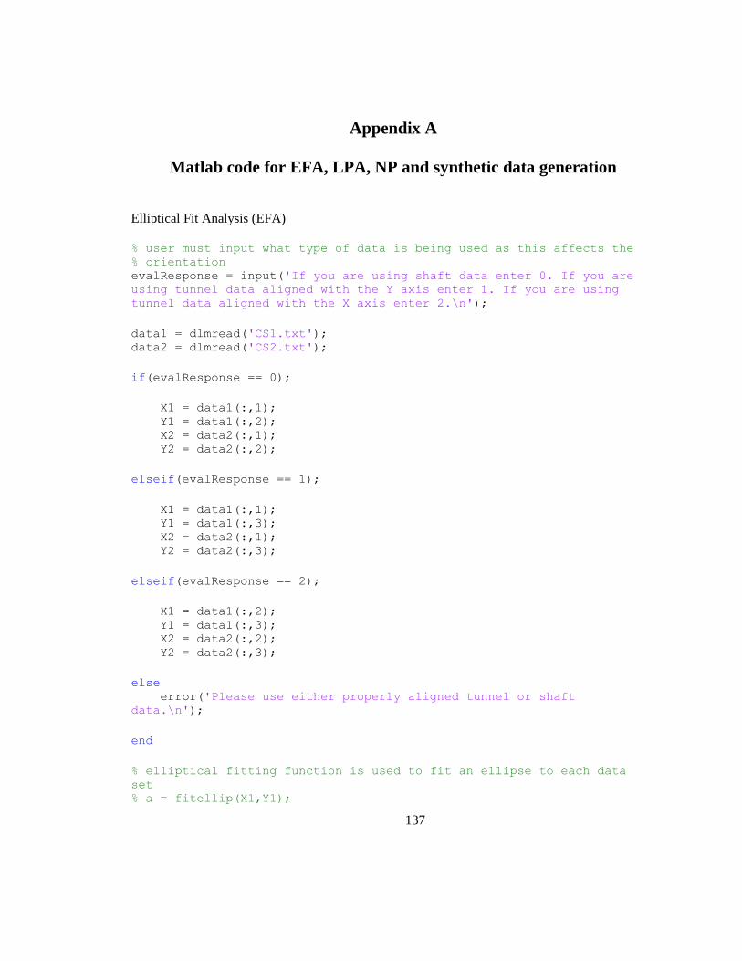
137
Appendix A
Matlab code for EFA, LPA, NP and synthetic data generation
Elliptical Fit Analysis (EFA)
% user must input what type of data is being used as this affects the % orientation evalResponse = input('If you are using shaft data enter 0. If you are
using tunnel data aligned with the Y axis enter 1. If you are using
tunnel data aligned with the X axis enter 2.\n');
data1 = dlmread('CS1.txt'); data2 = dlmread('CS2.txt');
if(evalResponse == 0);
X1 = data1(:,1); Y1 = data1(:,2); X2 = data2(:,1); Y2 = data2(:,2);
elseif(evalResponse == 1);
X1 = data1(:,1); Y1 = data1(:,3); X2 = data2(:,1); Y2 = data2(:,3);
elseif(evalResponse == 2);
X1 = data1(:,2); Y1 = data1(:,3); X2 = data2(:,2); Y2 = data2(:,3);
else error('Please use either properly aligned tunnel or shaft
data.\n');
end
% elliptical fitting function is used to fit an ellipse to each data
set % a = fitellip(X1,Y1);
138
mx1 = mean(X1); my1 = mean(Y1); sx1 = (max(X1)-min(X1))/2; sy1 = (max(Y1)-min(Y1))/2; x1 = (X1-mx1)/sx1; y1 = (Y1-my1)/sy1;
% Build design matrix D1 = [ x1.*x1 x1.*y1 y1.*y1 x1 y1 ones(size(x1)) ];
% Build scatter matrix S1 = D1'*D1;
% Build 6x6 constraint matrix C1(6,6) = 0; C1(1,3) = -2; C1(2,2) = 1; C1(3,1) = -2;
% Solve eigensystem [gevec1, geval1] = eig(S1,C1);
% Find the negative eigenvalue [NegR1, NegC1] = find(geval1 < 0 & ~isinf(geval1));
% Extract eigenvector corresponding to positive eigenvalue A1 = gevec1(:,NegC1);
% unnormalize a1 = [ A1(1)*sy1*sy1, ... A1(2)*sx1*sy1, ... A1(3)*sx1*sx1, ... -2*A1(1)*sy1*sy1*mx1 - A1(2)*sx1*sy1*my1 + A1(4)*sx1*sy1*sy1, ... -A1(2)*sx1*sy1*mx1 - 2*A1(3)*sx1*sx1*my1 + A1(5)*sx1*sx1*sy1, ... A1(1)*sy1*sy1*mx1*mx1 + A1(2)*sx1*sy1*mx1*my1 +
A1(3)*sx1*sx1*my1*my1 ... - A1(4)*sx1*sy1*sy1*mx1 - A1(5)*sx1*sx1*sy1*my1 ... + A1(6)*sx1*sx1*sy1*sy1 ... ]';
% a = fitellip(X2,Y2); mx2 = mean(X2); my2 = mean(Y2); sx2 = (max(X2)-min(X2))/2; sy2 = (max(Y2)-min(Y2))/2; x2 = (X2-mx2)/sx2; y2 = (Y2-my2)/sy2;
% Build design matrix D2 = [ x2.*x2 x2.*y2 y2.*y2 x2 y2 ones(size(x2)) ];
139
% Build scatter matrix S2 = D2'*D2;
% Build 6x6 constraint matrix C2(6,6) = 0; C2(1,3) = -2; C2(2,2) = 1; C2(3,1) = -2;
% Solve eigensystem [gevec2, geval2] = eig(S2,C2);
% Find the negative eigenvalue [NegR2, NegC2] = find(geval2 < 0 & ~isinf(geval2));
% Extract eigenvector corresponding to positive eigenvalue A2 = gevec2(:,NegC2);
% unnormalize a2 = [ A2(1)*sy2*sy2, ... A2(2)*sx2*sy2, ... A2(3)*sx2*sx2, ... -2*A2(1)*sy2*sy2*mx2 - A2(2)*sx2*sy2*my2 + A2(4)*sx2*sy2*sy2, ... -A2(2)*sx2*sy2*mx2 - 2*A2(3)*sx2*sx2*my2 + A2(5)*sx2*sx2*sy2, ... A2(1)*sy2*sy2*mx2*mx2 + A2(2)*sx2*sy2*mx2*my2 +
A2(3)*sx2*sx2*my2*my2 ... - A2(4)*sx2*sy2*sy2*mx2 - A2(5)*sx2*sx2*sy2*my2 ... + A2(6)*sx2*sx2*sy2*sy2 ... ]';
% get ellipse orientation theta1 = atan2(a1(2),a1(1)-a1(3))/2;
% get scaled major/minor axes ct1 = cos(theta1); st1 = sin(theta1); ap1 = a1(1)*ct1*ct1 + a1(2)*ct1*st1 + a1(3)*st1*st1; cp1 = a1(1)*st1*st1 - a1(2)*ct1*st1 + a1(3)*ct1*ct1;
% get translations T1 = [[a1(1) a1(2)/2]' [a1(2)/2 a1(3)]']; t1 = -inv(2*T1)*[a1(4) a1(5)]'; cx1 = t1(1); cy1 = t1(2);
% get scale factor val1 = t1'*T1*t1; scale1 = 1 / (val1- a1(6));
140
% get major/minor axis radii r11 = 1/sqrt(scale1*ap1); r21 = 1/sqrt(scale1*cp1); v1 = [r11 r21 cx1 cy1 theta1]';
% get ellipse orientation theta2 = atan2(a2(2),a2(1)-a2(3))/2;
% get scaled major/minor axes ct2 = cos(theta2); st2 = sin(theta2); ap2 = a2(1)*ct2*ct2 + a2(2)*ct2*st2 + a2(3)*st2*st2; cp2 = a2(1)*st2*st2 - a2(2)*ct2*st2 + a2(3)*ct2*ct2;
% get translations T2 = [[a2(1) a2(2)/2]' [a2(2)/2 a2(3)]']; t2 = -inv(2*T2)*[a2(4) a2(5)]'; cx2 = t2(1); cy2 = t2(2);
% get scale factor val2 = t2'*T2*t2; scale2 = 1 / (val2- a2(6));
% get major/minor axis radii r12 = 1/sqrt(scale2*ap2); r22 = 1/sqrt(scale2*cp2); v2 = [r12 r22 cx2 cy2 theta2]';
dat = [v1 v2];
figure(1) t = uitable; cnames = {'Ellipse 1', 'Ellipse 2'}; rnames = {'Length of Minor Axis (m)', 'Length of Major Axis (m)',
'Centre of Ellipse x-coord', 'Centre of Ellipse y-coord', 'Theta'}; set(t, 'Data', dat, 'ColumnName', cnames, 'RowName', rnames,
'ColumnWidth', {78}, 'Position', [80 80 435 120]); annotation(figure(1),'textbox', [0.15 0.48 0.78 0.078],
'String',{'Properties of Ellipses Best Fit to LiDAR Data'},
'HorizontalAlignment','center', 'FontSize',12, 'FitBoxToText','off',
'LineStyle','none', 'EdgeColor','none'); saveas(1, 'EO Figure 1.jpg');
figure(2) plot(X1,Y1,'.g', X2,Y2,'.r'); axis equal; xlabel('width (m)', 'FontSize', 12);
141
ylabel('height (m)', 'FontSize', 12); title('Two Cross Sections of LiDAR Data for
Comparison','FontWeight','bold','FontSize', 14); legend('Cross Section 1', 'Cross Section 2', 'Location', 'SouthEast'); set(gcf, 'Color', 'w'); saveas(2, 'EO Figure 2.jpg');
% create best fit ellipse data set for first best fit N1 = 100; % this number of points can be changed dx1 = 2*pi/N1; elliptheta1 = v1(5); Rad1 = [[cos(elliptheta1) sin(elliptheta1)]', [-sin(elliptheta1)
cos(elliptheta1)]']; for i = 1:N1 ang1 = i*dx1; x1 = v1(1)*cos(ang1); y1 = v1(2)*sin(ang1); d11 = Rad1*[x1 y1]'; ellipX1(i) = d11(1) + v1(3); ellipY1(i) = d11(2) + v1(4); end
figure(3) plot(X1,Y1,'.g', ellipX1, ellipY1, 'b'); axis equal; xlabel('width (m)', 'FontSize', 12); ylabel('height (m)', 'FontSize', 12); title('Cross Section 1 Fit With
Ellipse','FontWeight','bold','FontSize', 14); legend('Cross Section 1', 'Ellipse Fit', 'Location', 'SouthEast'); set(gcf, 'Color', 'w'); saveas(3, 'EO Figure 3.jpg');
% create best fit ellipse data set for second best fit N2 = 100; dx2 = 2*pi/N2; elliptheta2 = v2(5); Rad2 = [[cos(elliptheta2) sin(elliptheta2)]', [-sin(elliptheta2)
cos(elliptheta2)]']; for i = 1:N2 ang2 = i*dx2; x2 = v2(1)*cos(ang2); y2 = v2(2)*sin(ang2); d12 = Rad2*[x2 y2]'; ellipX2(i) = d12(1) + v2(3); ellipY2(i) = d12(2) + v2(4); end
figure(4)

142
plot(X2,Y2,'.r', ellipX2, ellipY2, 'b'); axis equal; xlabel('width (m)', 'FontSize', 12); ylabel('height (m)', 'FontSize', 12); title('Cross Section 2 Fit With
Ellipse','FontWeight','bold','FontSize', 14); legend('Cross Section 2', 'Ellipse Fit', 'Location', 'SouthEast'); set(gcf, 'Color', 'w'); saveas(4, 'EO Figure 4.jpg');
% centre of ellipse is used to translate each data set so it is centred % about the origin newX1 = ellipX1 - v1(3); newY1 = ellipY1 - v1(4); newX2 = ellipX2 - v2(3); newY2 = ellipY2 - v2(4);
x1 = linspace(0, max(newX1), 100); x2 = linspace(0, max(newY1), 100);
m1 = 0; m2 = 0;
angle1 = abs(v1(5) + pi/2); angle2 = abs(v2(5) + pi/2);
circtest1 = abs(v1(1)-v1(2)); circtest2 = abs(v2(1)-v2(2));
if (circtest1 < 0.00015); m1 = 0; y1 = m1*x1; a = 1; else if (angle1 < 0.0001);
m1 = 0; y1 = m1*x1; a = 2; else if (abs(1 - (angle1/(pi/2))) < 0.0001);
y1 = x1; x1 = zeros(size(x1)); a = 3; else if (abs(1 - (angle1/pi)) < 0.00001);
m1 = 0; y1 = m1*x1; a = 4;
143
else
m1 = tan(v1(5) + pi/2); y1 = m1*x1; a = 5; end end end end
if (circtest2 < 0.00015); m2 = 0; y2 = m2*x2; b = 1; else if (angle2 < 0.0001);
m2 = 0; y2 = m2*x2; b = 2; else if (abs(1 - (angle2/(pi/2))) < 0.0001);
y2 = x2; x2 = zeros(size(x2)); b = 3; else if (abs(1 - (angle2/pi)) < 0.0001);
m2 = 0; y2 = m2*x2; b = 4; else
m2 = tan(v2(5) + pi/2); y2 = m2*x2; b = 5; end end end end
% calculate the volumes enclosed by the best fit ellipses vol1 = abs(v1(1)*v1(2)*pi); vol2 = abs(v2(1)*v2(2)*pi);
figure (5) plot(newX1, newY1, '-g', x1, y1, '--g', newX2, newY2, '-r', x2, y2, '--
r');
144
axis equal; xlabel('width (m)', 'FontSize', 12); ylabel('height (m)', 'FontSize', 12); title('Comparison of two Ellipse Fits', 'FontWeight', 'bold',
'FontSize', 14); legend('Ellipse 1', 'Long Axis Orientation of Ellipse 1', 'Ellipse 2',
' Long Axis Orientation of Ellipse 2', 'Location', 'NorthEastOutside'); xlim([min(ellipX1)-1 max(ellipX1)+1]); ylim([min(ellipY1)-1 max(ellipY1)+1]); set(gcf, 'Color', 'w'); text(max(ellipX1)+2, min(ellipY1), sprintf('Ellipse 1 = %0.3f m^2,
Ellipse 2 = %0.3f m^2', vol1, vol2)); saveas(5, 'EO Figure 5.jpg');
[theta1, rho1] = cart2pol(newX1, newY1); [theta2, rho2] = cart2pol(newX2, newY2);
theta1 = theta1'; theta2 = theta2'; rho1 = rho1'; rho2 = rho2'; E1 = [theta1, rho1]; E2 = [theta2, rho2]; E1 = sortrows(E1,1); E2 = sortrows(E2,1);
theta1 = E1(:,1)'; theta2 = E2(:,1)'; rho1 = E1(:,2)'; rho2 = E2(:,2)';
% determine the chang between the two LiDAR profiles change = rho1 - rho2;
% chose an exaggeration to display the deformations at stretch = input('By how many times would you like the deformations
exaggerated?\n'); stretchdef = change*stretch; def = rho1 - stretchdef;
[defX, defY] = pol2cart(theta1, def);
figure (6) plot(newX1, newY1, 'g'); hold on; plot(defX,defY, 'Color', [0.5 0 .5], 'LineWidth', 2); axis equal; title('Change in Ellipse from First Fit Profile', 'FontWeight', 'bold',
'FontSize', 14);
145
legend('Ellipse fit 1', 'Change in ellipse profile'); xlim([min(newX1)-.5 max(newX1)+.5]); ylim([min(newY1)-.5 max(newY1)+.5]); set(gcf, 'Color', 'w'); saveas(6, 'EO Figure 6.jpg');
% determine diametric change acrossdiam = round((length(change)/2)) + 1; deform = zeros(1, length(change)/2); newtheta = zeros(1, length(change)/2);
for i = 1:(length(change)/2) deform(i) = change(i) + change(acrossdiam); acrossdiam = acrossdiam + 1; newtheta(i) = theta1(i); end
figure (7) plot(newtheta, deform, 'Color', [.5 0 .5], 'LineWidth', 2); xlabel('Distance around tunnel (m) clockwise from sidewall',
'FontSize', 12); ylabel('Total displacement (m) [positive is inwards movement]',
'FontSize', 12); title('Diametric tunnel displacement profile', 'FontWeight', 'bold',
'FontSize', 14); legend('Displacement profile', 'Location', 'NorthEastOutside'); set(gcf, 'Color', 'w'); line([-pi,0], [0, 0], 'Color', 'k'); xlim([min(newtheta),0]); saveas(7, 'EO Figure 7.jpg');
146
LiDAR Profile Analysis (LPA)
% user must input what type of data is being used as this affects the % orientation evalResponse = input('If you are using shaft data enter 0. If you are
using tunnel data aligned with the Y axis enter 1. If you are using
tunnel data aligned with the X axis enter 2.\n'); format long g;
data1 = dlmread('CS1.txt'); data2 = dlmread('CS2.txt');
if(evalResponse == 0)
X1 = data1(:,1); Y1 = data1(:,2); X2 = data2(:,1); Y2 = data2(:,2);
elseif(evalResponse == 1);
X1 = data1(:,1); Y1 = data1(:,3); X2 = data2(:,1); Y2 = data2(:,3);
elseif(evalResponse == 2);
X1 = data1(:,2); Y1 = data1(:,3); X2 = data2(:,2); Y2 = data2(:,3);
else
error('Please use either properly aligned tunnel or shaft
data.\n');
end
% elliptical fitting function is used to fit an ellipse to each data
set a = fitellip(X1,Y1); b = fitellip(X2,Y2);
% function is used to solve for parameters that define best fit ellipse v1 = solveellipse(a);
147
v2 = solveellipse(b);
cx1 = v1(3); cy1 = v1(4); cx2 = v2(3); cy2 = v2(4);
% centre of ellipse is used to translate each data set so it is centred % about the origin X1 = X1 - cx1; Y1 = Y1 - cy1; X2 = X2 - cx2; Y2 = Y2 - cy2;
[theta1, rho1] = cart2pol(X1,Y1); [theta2, rho2] = cart2pol(X2,Y2);
figure(1) plot(X1,Y1,'.g', X2,Y2,'.r'); axis equal; xlabel('width (m)', 'FontSize', 12); ylabel('height (m)', 'FontSize', 12); title('Two Cross Sections of LiDAR Data for
Comparison','FontWeight','bold','FontSize', 14); legend('Cross Section 1', 'Cross Section 2', 'Location', 'SouthEast'); set(gcf, 'Color', 'w'); saveas(1, 'ULS Figure 1.jpg');
% create best fit ellipse data set for first best fit N1 = 100; % this number of points can be changed dx1 = 2*pi/N1; elliptheta1 = v1(5); Rad1 = [[cos(elliptheta1) sin(elliptheta1)]', [-sin(elliptheta1)
cos(elliptheta1)]'];
for i = 1:N1
ang1 = i*dx1;
x1 = v1(1)*cos(ang1); y1 = v1(2)*sin(ang1);
d11 = Rad1*[x1 y1]';
ellipX1(i) = d11(1); ellipY1(i) = d11(2);
end
148
figure(2) plot(X1,Y1,'.g', ellipX1, ellipY1, 'b'); axis equal; xlabel('width (m)', 'FontSize', 12); ylabel('height (m)', 'FontSize', 12); title('Cross Section 1 Fit With
Ellipse','FontWeight','bold','FontSize', 14); legend('Cross Section 1', 'Ellipse Fit', 'Location', 'SouthEast'); set(gcf, 'Color', 'w'); saveas(2, 'ULS Figure 2.jpg');
% create best fit ellipse data set for second best fit N2 = 100; dx2 = 2*pi/N2; elliptheta2 = v2(5); Rad2 = [[cos(elliptheta2) sin(elliptheta2)]', [-sin(elliptheta2)
cos(elliptheta2)]'];
for i = 1:N2
ang2 = i*dx2;
x2 = v2(1)*cos(ang2); y2 = v2(2)*sin(ang2);
d12 = Rad2*[x2 y2]';
ellipX2(i) = d12(1); ellipY2(i) = d12(2);
end
figure(3) plot(X2,Y2,'.r', ellipX2, ellipY2, 'b'); axis equal; xlabel('width (m)', 'FontSize', 12); ylabel('height (m)', 'FontSize', 12); title('Cross Section 2 Fit With
Ellipse','FontWeight','bold','FontSize', 14); legend('Cross Section 2', 'Ellipse Fit', 'Location', 'SouthEast'); set(gcf, 'Color', 'w'); saveas(3, 'ULS Figure 3.jpg');
figure(4) plot(theta1,rho1,'.g'); xlabel('Theta', 'FontSize', 12); ylabel('Radius (m)', 'FontSize', 12);
149
title('Unrolled Profile of Cross Section
1','FontWeight','bold','FontSize', 14); set(gcf, 'Color', 'w'); saveas(4, 'ULS Figure 4.jpg');
figure(5) plot(theta2,rho2,'.r'); xlabel('Theta', 'FontSize', 12); ylabel('Radius (m)', 'FontSize', 12); title('Unrolled Profile of Cross Section
2','FontWeight','bold','FontSize', 14); set(gcf, 'Color', 'w'); saveas(5, 'ULS Figure 5.jpg');
% a filter cutoff is used to filter anomolies from the interior of the
data % set, closest points are filtered evalResponse = input('Enter the filter cutoff % (enter 100 to use all
data)\n');
nwindows = 5; % the number of filter windows must be optimized based on
the type of anomolies present
if(evalResponse == 100)
else counter1 = 1; counter2 = 2;
windowwidth1 = round(length(theta1)/nwindows); windowwidth2 = round(length(theta2)/nwindows);
for i = 1:nwindows
if(counter1*windowwidth1 > length(theta1))
else
temp = sortrows([theta1((windowwidth1*(counter1-
1)+1):counter1*windowwidth1),rho1((windowwidth1*(counter1-
1)+1):counter1*windowwidth1)],2); temp(1:round(((100-evalResponse)*windowwidth1)/100),:) = 0;
theta1((windowwidth1*(counter1-1)+1):counter1*windowwidth1)
= temp(:,1); rho1((windowwidth1*(counter1-1)+1):counter1*windowwidth1) =
temp(:,2);
150
counter1 = counter1 + 1;
end
end
for i = 1:nwindows
if(counter2*windowwidth2 > length(theta2))
else
temp = sortrows([theta2((windowwidth2*(counter2-
1)+1):counter2*windowwidth2),rho2((windowwidth2*(counter2-
1)+1):counter2*windowwidth2)],2); temp(1:round(((100-evalResponse)*windowwidth2)/100),:) = 0;
theta2((windowwidth2*(counter2-1)+1):counter2*windowwidth2)
= temp(:,1); rho2((windowwidth2*(counter2-1)+1):counter2*windowwidth2) =
temp(:,2);
counter2 = counter2 + 1;
end
end
end
theta1 = nonzeros(theta1); theta2 = nonzeros(theta2); rho1 = nonzeros(rho1); rho2 = nonzeros(rho2);
[junk index] = unique(theta1,'first'); theta1 = theta1(sort(index)); rho1 = rho1(sort(index));
[junk index] = unique(theta2,'first'); theta2 = theta2(sort(index)); rho2 = rho2(sort(index));
regtheta = linspace(min(theta1),max(theta1),length(theta1));
newrho2 = interp1(theta2,rho2,regtheta);
151
newrho1 = interp1(theta1,rho1,regtheta);
logical1 = isnan(newrho1); logical2 = isnan(newrho2);
newrho1(logical1 == 1) = []; newrho1(logical2 == 1) = []; newrho2(logical1 == 1) = []; newrho2(logical2 == 1) = []; regtheta(logical1 == 1) = []; regtheta(logical2 == 1) = [];
% find the difference between the data sets diff = newrho1 - newrho2;
evalResponse = input('By how many times would you like the deformations
exaggerated?\n');
stretchfactor = evalResponse; stretchdiff = diff.*stretchfactor; rhodef = newrho1 - stretchdiff;
[defx, defy] = pol2cart(regtheta,rhodef);
deforms = [regtheta; rhodef]; addstep = length(regtheta)/2; lengthstretch = length(regtheta);
% need to evaluate diametric displacement if(mod(lengthstretch,2)==0)
rhodefdiam = zeros(1,length(stretchdiff)/2);
for i = 1:length(rhodefdiam)
rhodefdiam(i) = stretchdiff(i) +
stretchdiff((length(stretchdiff)/2) + i);
end
else
rhodefdiam = zeros(1,(length(stretchdiff)-1)/2);
for i = 1:length(rhodefdiam)
152
rhodefdiam(i) = stretchdiff(i) +
stretchdiff(((length(stretchdiff)-1)/2) + i);
end
end
if(mod(lengthstretch,2)==0)
regthetadiam = regtheta(1:length(regtheta)/2);
else
regthetadiam = regtheta(1:(length(regtheta)-1)/2);
end
% determine the average diametric displacement, the standard deviation,
and % the variance of displacement disp = rhodefdiam/stretchfactor; avg_disp = mean(disp); std_dev = std(disp); variance = var(disp);
figure (6) plot(regthetadiam, disp, '.', 'Color', [.5 0 .5]); xlabel('Distance around tunnel (m) clockwise from sidewall',
'FontSize', 12); ylabel('Total displacement (m) [positive is inwards movement]',
'FontSize', 12); title('Diametric tunnel displacement profile', 'FontWeight', 'bold',
'FontSize', 14); legend('Displacement profile', 'Location', 'NorthEastOutside'); text(0.1, max(disp)-(max(disp)/10), sprintf('Average displacement
(diametric): %0.3f m', avg_disp)); text(0.1, max(disp)-(max(disp)/10)*2, sprintf('Standard deviation:
%0.3f m', std_dev)); % text(0.1, max(disp)-(max(disp)/10)*3, sprintf('Variance: %0.3f m',
variance)); set(gcf, 'Color', 'w'); line([-pi,0], [0, 0], 'Color', 'k'); xlim([min(regthetadiam),0]); saveas(6, 'ULS Figure 6.jpg');
figure(7) plot(X1,Y1,'.g');
153
hold on; plot(defx,defy,'.', 'Color', [.5 0 .5]); axis equal; xlabel('width (m)', 'FontSize', 12); ylabel('height (m)', 'FontSize', 12); title({'Cross Section 1 with Amount of Change';'Compared to Cross
Seciton 2'},'FontWeight','bold','FontSize', 14); legend('Cross Section 1', 'Change between CS1 and CS2', 'Location',
'SouthEast'); set(gcf, 'Color', 'w'); hold off; saveas(7, 'ULS Figure 7.jpg');
dtheta = regtheta(2)-regtheta(1);
R = newrho1;
% determine the volumes of convergence and the locations that limit
areas % of convergence and divergence\ area = zeros(1,10000); crossoverpoints = zeros(2,10000); changei = zeros(1,10000);
areacount = 1;
if(isempty(nonzeros(diff))) error('There is no change in the data therefore volume changes can
not be calculated or displayed.\n'); else
for i = 1:(length(regtheta)-1)
area(areacount) = area(areacount) + dtheta*R(i)*diff(i);
if(abs(sign(diff(i+1))-sign(diff(i))) > 1 || sign(diff(i)) ==
0)
areacount = areacount + 1; crossoverpoints(:,areacount) = [regtheta(i); newrho1(i)]; changei(areacount) = i;
end
end end
area = nonzeros(area)';
154
logicalcrossover1 = (crossoverpoints(1,:) == 0); logicalcrossover2 = (crossoverpoints(2,:) == 0);
logicalcrossover = logicalcrossover1.*logicalcrossover2;
crossoverpoints(:,logicalcrossover == 1) = []; changei(logicalcrossover == 1) = [];
if(sign(diff(1)) == sign(diff(end)))
if(length(area) ~= 1)
area(1) = area(1) + area(end); area(end) = [];
end
end
minarea = input('Minimum area change to consider (in m^2)?\n');
logicalminarea = abs(area) < minarea; area(logicalminarea == 1) = []; crossoverpoints(:,logicalminarea == 1) = []; changei(logicalminarea == 1) = [];
[crossx crossy] = pol2cart(crossoverpoints(1,:),crossoverpoints(2,:)); [newX1,newY1] = pol2cart(regtheta,newrho1);
figure(8) plot(X1,Y1,'.g',X2,Y2,'.r'); axis equal; xlabel('width (m)', 'FontSize', 12); ylabel('height (m)', 'FontSize', 12); title('Deformed Area Locations and Volumes Plotted on LiDAR
Profiles','FontWeight','bold','FontSize', 14); legend('CS1', 'CS2','Location', 'SouthEast'); set(gcf, 'Color', 'w'); saveas(8, 'ULS Figure 8.jpg');
for i = 1:length(crossx)
text(crossx(i),crossy(i),sprintf(' %0.3f , %0.3f
',crossx(i),crossy(i)),'HorizontalAlignment','center','BackgroundColor'
,[0.8 0.8 0.8],'EdgeColor',[0.8 0.8 0.8]);
155
if(i == 1)
text(mean([newX1(round(mean([changei(i),(length(defx)-
changei(end))]))),defx(round(mean([changei(i),(length(defx)-
changei(end))])))]),mean([newY1(round(mean([changei(i),(length(defx)-
changei(end))]))),defy(round(mean([changei(i),(length(defx)-
changei(end))])))]),sprintf(' %0.3f m^2
',area(i)),'HorizontalAlignment','center','BackgroundColor',[1 1
1],'EdgeColor',[0 0 0]);
else
text(mean([newX1(round(mean([changei(i),changei(i-
1)]))),defx(round(mean([changei(i),changei(i-
1)])))]),mean([newY1(round(mean([changei(i),changei(i-
1)]))),defy(round(mean([changei(i),changei(i-1)])))]),sprintf(' %0.3f
m^2 ',area(i)),'HorizontalAlignment','center','BackgroundColor',[1 1
1],'EdgeColor',[0 0 0]);
end
end
if(isempty(crossx))
text(0,0,sprintf(' %0.3f m^2',
area),'HorizontalAlignment','center','BackgroundColor',[0.8 0.8
0.8],'EdgeColor',[0.8 0.8 0.8]);
end
156
Noise Profile (NP)
%interpolation for noise and moving average calc max_theta = max(regthetadiam); num_interps = length(disp); length_interp = linspace(-pi,0,num_interps); new_deform = interp1(newtheta, deform, length_interp); noise_calcplot = new_deform - disp;
% moving average calculation for LiDAR profile data pt_avgs = input('What number of points would you like to use for the
moving average?\n'); num_avgs = round(length(disp)/pt_avgs)-1; first_seed = round(pt_avgs/2); moving_average = zeros(1, num_avgs); movavg_theta = zeros(1, num_avgs); temp = zeros(1, pt_avgs); pt_avg_count = 1; pt_avgs2 = pt_avgs;
for i = 1:num_avgs start = pt_avg_count; finish = pt_avgs2; temp = disp(start:finish); moving_average(i) = sum(temp)/pt_avgs; movavg_theta(i) = regthetadiam(first_seed); pt_avg_count = pt_avg_count + pt_avgs; pt_avgs2 = pt_avgs2 + pt_avgs; first_seed = first_seed + pt_avgs; end
plot(regthetadiam, noise_calcplot, 'Color', [0.5 0 0.5]); hold on; plot(newtheta, deform, 'Color', [0 .8 0.2], 'LineWidth', 2); plot(movavg_theta, moving_average, '-or', 'LineWidth', 1); xlabel('Angle around tunnel', 'FontSize', 12); ylabel('Total displacement (m) [positive is inwards movement]',
'FontSize', 12); title('Deviation from Best Fit Ellipse', 'FontWeight', 'bold',
'FontSize', 14); set(gcf, 'Color', 'w'); line([-pi,0], [0, 0], 'Color', 'k'); xlim([min(regthetadiam),0]);
format short;
% determine the max, min, avg, and std deviation of diametric
convergence
157
% measured from the compaison of the elliptical best fit profiles as
well % as the volume change max_diam_conv_ellip = max(deform); min_diam_conv_ellip = min(deform); avg_diam_conv_ellip = mean(deform); std_diam_conv_ellip = std(deform); vol_change_ellip = vol1 - vol2;
% determine the max, min, avg, and std deviation of diametric
convergence % measured from the compaison of the LiDAR profiles as well % as the volume change max_diam_conv_lidar = max(disp); min_diam_conv_lidar = min(disp); avg_diam_conv_lidar = mean(disp); std_diam_conv_lidar = std(disp); vol_change_lidar = sum(area); empty = isempty(area); if empty ==1 vol_change_lidar = 0; else end
max_syst_deviat = max(noise_calcplot); min_syst_deviat = min(noise_calcplot);
if abs(max_syst_deviat) >= abs(min_syst_deviat); max_syst_deviat = abs(max_syst_deviat); else max_syst_deviat = abs(min_syst_deviat); end
logic_noise = isnan(noise_calcplot); noise_calcplot(logic_noise == 1) = [];
noise = std(noise_calcplot);
misfit = zeros(1, length(new_deform));
for i = 1:length(disp) misfit(i) = (disp(i) - new_deform(i))^2; end
logic1 = isnan(misfit); misfit(logic1 == 1) = [];
RMS = sqrt(sum(misfit)/length(misfit));

158
Excel = [ max_diam_conv_ellip max_diam_conv_lidar min_diam_conv_ellip
min_diam_conv_lidar avg_diam_conv_ellip avg_diam_conv_lidar
std_diam_conv_ellip std_diam_conv_lidar vol_change_ellip
vol_change_lidar RMS max_syst_deviat]'
159
Synthetic Data Generator
clear % user is asked for input values to create synthetic data set A = input('How many data points would you like to use?\n'); radius = input('What is the radius of tunnel you would like\nto
generate data for (in m)?\n'); std_noise = input('What is the standard deviation of the noise (in
m)?\n');
syst_noise = input('Would you like to include systematic noise (enter 1
for yes)?\n');
if (syst_noise == 1) % beta is the magnitude of the maximum systematic deviation beta = input('What beta would you like to use?\n'); % gamma is the number of systematic deviations gamma = input('What gamma would you like to use (must be >2)?\n'); end
squish = input('Would you like to skew or rotate data (enter 1 for
yes)?\n');
if (squish == 1) % skew is the amount of extension of the long axis and shrinking of
the % short axis skew = input('What level of elliptical skew would you like to\nadd
to the data (m)?\n'); rotate = input('What rotation would you like to give the data (in
radians ccw)?\n'); end
occlude = input('Would you like to occlude data (enter 1 for yes)?\n');
if (occlude == 1) percent_occlude = input('What percent of your data would you like
occluded?\n'); avg_length_occlude = input('What would you like the average length
of an occluded\nsection to be (in m)?\n'); std_occlude = input('What would you like the standard deviation of
an occluded\nsections length to be (in m)?\n'); end
CS = input('Is this CS1 data or CS2 data?\n');
% create a data set with the number of points input by the user theta = linspace(0, 2*pi, A);
160
% convert this data set to x and y coordinates x = radius*cos(theta); y = radius*sin(theta);
% add random noise to the data based on the specified standard
deviation % input by the user noise = random('Normal',0, std_noise, A, 1);
% systematic noise is created if (syst_noise == 1) for n = 1:A x_noise(n) = (radius + noise(n) +
beta*cos(gamma*theta(n)))*cos(theta(n)); end
for n = 1:A y_noise(n) = (radius + noise(n)+
beta*cos(gamma*theta(n)))*sin(theta(n)); end
else for n = 1:A x_noise(n) = (radius + noise(n))*cos(theta(n)); end
for n = 1:A y_noise(n) = (radius + noise(n))*sin(theta(n)); end end
% skew is added to the data if (squish == 1) max_skew = radius + skew; min_skew = radius - skew;
x_skew = x_noise; y_skew = y_noise;
for n = 1:A x_skew(n) = (x_noise(n)/radius)*min_skew; end
for n = 1:A y_skew(n) = (y_noise(n)/radius)*max_skew; end
161
[thetay_final, rho1] = cart2pol(x_skew, y_skew);
% data is rotated if a rotation is present for n = 1:A thetay_final(n) = thetay_final(n) + rotate; end
for n = 1:A if(thetay_final(n) <= 2*pi)
else thetay_final(n) = thetay_final(n) - 2*pi; end end
[x_rot, y_rot] = pol2cart(thetay_final, rho1);
else x_rot = x_noise; y_rot = y_noise; end
% data is occluded if occlusion is entered if (occlude == 1) avg_pts_occlude = avg_length_occlude*(A/(2*pi*radius)); std_pts = std_occlude*(A/(2*pi*radius)); num_occlude_seeds = (percent_occlude/100)*A/avg_pts_occlude; prob_seed = num_occlude_seeds/A;
tol = 0.05; x_final = x_rot; y_final = y_rot;
while((length(x_final) > (A*(1-percent_occlude/100)+tol*A)) ||
(length(x_final) < (A*(1-percent_occlude/100)-tol*A)))
x_final = x_rot; y_final = y_rot;
randnums = random('unif',0,100,A,1); logical = randnums <= prob_seed*100; start_pts = find(logical);
occlude_lengths = zeros(1,nnz(start_pts)); start = zeros(1,nnz(start_pts));
count = 1; current_count = 100000000;
162
hit_first_seed = 0;
occlude_data = zeros(1,A);
for i = 1:A
if(count <= length(start_pts))
if(start_pts(count) == i)
occlude_lengths(count) =
round(normrnd(avg_pts_occlude,std_pts));
start(count) = i; current_count = 1; count = count + 1;
hit_first_seed = 1;
end
end
if(hit_first_seed == 1)
if(current_count <= occlude_lengths(count-1))
occlude_data(i) = 1;
end
current_count = current_count + 1;
end
end
x_final(occlude_data == 1) = []; y_final(occlude_data == 1) = [];
end
else x_final = x_rot; y_final = y_rot; end
163
X = x_final'; Y = y_final'; CS_data = [X Y];
% data is written to a text file and saved if(CS == 1) dlmwrite('CS1.txt', CS_data); elseif (CS == 2) dlmwrite('CS2.txt', CS_data); else error('Please either choose 1 or 2.\n'); end
figure(1) plot(x_final,y_final,'.b','MarkerSize',15); axis equal; xlabel('width of tunnel (m)'); ylabel('height of tunnel (m)'); title('Synthetic tunnel data'); ylim([min(y_final)-2, max(y_final)+2]); xlim([min(x_final)-2, max(x_final)+2]); set(gcf, 'Color', 'w');
164
Synthetic Data Analysis
% example of creation and testing of multiple synthetic data sets for
MACE, % MICE, ACE analysis radnom = 5; circumf = pi*radnom*radnom;
Synthfunc(5500,radnom,0,0,0,0,0,0,0,0,1);
rad2 = 4.9:0.0005:4.995;
% rad2 = radnom - 0.005;
std_noise = 0:0.001:0.05;
beta = 0; gamma = 0; k=1:7;
maxdisp = zeros(length(std_noise),length(rad2), length(k)); mindisp = zeros(length(std_noise),length(rad2), length(k)); avgdisp = zeros(length(std_noise),length(rad2), length(k)); maxdeform = zeros(length(std_noise),length(rad2), length(k)); mindeform = zeros(length(std_noise),length(rad2), length(k)); avgdeform = zeros(length(std_noise),length(rad2), length(k) );
for(k=1:7)
for(i=1:length(std_noise))
for(j=1:length(rad2))
Synthfunc(5500,rad2(j),std_noise(i),beta,gamma,0,0,0,0,0,2)
[regthetadiam disp newtheta deform] = lidarfunc();
maxdisp(i,j,k) = maxdisp(i,j,k) + max(disp); mindisp(i,j,k) = mindisp(i,j,k) + min(disp); avgdisp(i,j,k) = avgdisp(i,j,k) + mean(disp); maxdeform(i,j,k) = maxdeform(i,j,k) + max(deform); mindeform(i,j,k) = mindeform(i,j,k) + min(deform); avgdeform(i,j,k) = avgdeform(i,j,k) + mean(deform);
end
end
165
end
maxdisp2d = zeros(length(std_noise),length(rad2)); mindisp2d = zeros(length(std_noise),length(rad2)); avgdisp2d = zeros(length(std_noise),length(rad2)); maxdeform2d = zeros(length(std_noise),length(rad2)); mindeform2d = zeros(length(std_noise),length(rad2)); avgdeform2d = zeros(length(std_noise),length(rad2));
stdmaxdisp2d = zeros(length(std_noise),length(rad2)); stdmindisp2d = zeros(length(std_noise),length(rad2)); stdavgdisp2d = zeros(length(std_noise),length(rad2)); stdmaxdeform2d = zeros(length(std_noise),length(rad2)); stdmindeform2d = zeros(length(std_noise),length(rad2)); stdavgdeform2d = zeros(length(std_noise),length(rad2));
for(i=1:length(std_noise)) for(j=1:length(rad2)) maxdisp2d(i,j) = mean(maxdisp(i,j,:)); mindisp2d(i,j) = mean(mindisp(i,j,:)); avgdisp2d(i,j) = mean(avgdisp(i,j,:)); maxdeform2d(i,j) = mean(maxdeform(i,j,:)); mindeform2d(i,j) = mean(mindeform(i,j,:)); avgdeform2d(i,j) = mean(avgdeform(i,j,:));
stdmaxdisp2d(i,j) = std(maxdisp(i,j,:)); stdmindisp2d(i,j) = std(mindisp(i,j,:)); stdavgdisp2d(i,j) = std(avgdisp(i,j,:)); stdmaxdeform2d(i,j) = std(maxdeform(i,j,:)); stdmindeform2d(i,j) = std(mindeform(i,j,:)); stdavgdeform2d(i,j) = std(avgdeform(i,j,:)); end end
%need to use rad2sized if the length of rad2 is greater than 1 rad2sized = zeros(length(std_noise),length(rad2));
for(m = 1:length(std_noise))
rad2sized(m,:) = rad2';
end
diffmaxdisp = maxdisp2d - (radnom - rad2sized)*2; diffmindisp = mindisp2d - (radnom - rad2sized)*2; diffavgdisp = avgdisp2d - (radnom - rad2sized)*2;
166
diffmaxdeform = maxdeform2d - (radnom - rad2sized)*2; diffmindeform = mindeform2d - (radnom - rad2sized)*2; diffavgdeform = avgdeform2d - (radnom - rad2sized)*2;
raddiff = (radnom-rad2)*2;
[X1 X2] = meshgrid(raddiff, std_noise);
% disp is from LiDAR data, deform is from Elliptical data

167
Synthetic Data Analysis Figures
% Example of figures used for analysis of synthetic data figure (1) % Change error for the maximum diameter measurement from LPA contour3(X1,X2,diffmaxdisp,300); colormap jet; title('MACE from LPA','FontWeight','bold','FontSize', 14); axis([0 0.01 6000 11000 -0.04 0.04]); xlabel('Standard deviation of noise (m)', 'FontSize', 12); ylabel('Number of points', 'FontSize', 12); zlabel('MACE (m)', 'FontSize', 12); set(gcf, 'Color', 'w'); colorbar; ylims = get(colorbar, 'YLim'); set(colorbar, 'YTick', ylims, 'Position', [0.88 0.8 0.012 0.12]);
figure(2) % Change error for the maximum diameter measurement from EFA contour3(X1,X2,diffmaxdeform,300); colormap jet; title('MACE from EFA','FontWeight','bold','FontSize', 14); axis([4.9 5.0 0 0.06 -0.01 0.1]); xlabel('Standard deviation of noise (m)', 'FontSize', 12); ylabel('Number of points', 'FontSize', 12); zlabel('MACE (m)', 'FontSize', 12); set(gcf, 'Color', 'w'); colorbar; ylims = get(colorbar, 'YLim'); set(colorbar, 'YTick', ylims, 'Position', [0.88 0.8 0.012 0.12]);
figure(3)% Change error for the minimum diameter measurement from LPA contour3(X1,X2,diffmindisp, 300); colormap jet; title('MICE for LPA','FontWeight','bold','FontSize', 14); axis([4.9 5.0 0 0.06 -0.1 0.01]); xlabel('Standard deviation of noise (m)', 'FontSize', 12); ylabel('Number of points', 'FontSize', 12); zlabel('MICE (m)', 'FontSize', 12); set(gcf, 'Color', 'w'); colorbar; ylims = get(colorbar, 'YLim'); set(colorbar, 'YTick', ylims, 'Position', [0.88 0.8 0.012 0.12]);
figure(4)% Change error for the minimum diameter measurement from EFA contour3(X1,X2,diffmindeform, 300); colormap jet; title('MICE from EFA','FontWeight','bold','FontSize', 14); axis([4.9 5.0 0 0.06 -0.1 0.01]); xlabel('Standard deviation of noise (m)', 'FontSize', 12); ylabel('Number of points', 'FontSize', 12);
168
zlabel('MICE (m)', 'FontSize', 12); set(gcf, 'Color', 'w'); colorbar; ylims = get(colorbar, 'YLim'); set(colorbar, 'YTick', ylims, 'Position', [0.88 0.8 0.012 0.12]);
figure(5)% Change error for the average diameter measurement from LPA contour3(X1,X2,diffavgdisp, 300); colormap jet; title('ACE from LPA','FontWeight','bold','FontSize', 14); axis([4.9 5.0 0 0.06 -0.001 0.001]); xlabel('Standard deviation of noise (m)', 'FontSize', 12); ylabel('Number of points', 'FontSize', 12); zlabel('ACE (m)', 'FontSize', 12); set(gcf, 'Color', 'w'); colorbar; ylims = get(colorbar, 'YLim'); set(colorbar, 'YTick', ylims, 'Position', [0.88 0.8 0.012 0.12]);
figure(6)% Change error for the average diameter measurement from EFA contour3(X1,X2,diffavgdeform, 300); colormap jet; title('ACE from EFA','FontWeight','bold','FontSize', 14); axis([4.9 5.0 0 0.06 -0.001 0.001]); xlabel('Standard deviation of noise (m)', 'FontSize', 12); ylabel('Number of points', 'FontSize', 12); zlabel('ACE (m)', 'FontSize', 12); set(gcf, 'Color', 'w'); colorbar; ylims = get(colorbar, 'YLim'); set(colorbar, 'YTick', ylims, 'Position', [0.88 0.8 0.012 0.12]);
figure (7) % Standard deviation of MACE from LPA surf(X1,X2,stdmaxdisp2d); colormap jet; title('Standard deviation of MACE from
LPA','FontWeight','bold','FontSize', 14); axis([4.9 5.0 0 0.06 -0.001 0.001]); xlabel('Standard deviation of noise (m)', 'FontSize', 12); ylabel('Number of points', 'FontSize', 12); zlabel('Standard Deviation (m)', 'FontSize', 12); set(gcf, 'Color', 'w'); colorbar; ylims = get(colorbar, 'YLim'); set(colorbar, 'YTick', ylims, 'Position', [0.88 0.8 0.012 0.12]);
figure(8) % Standard deviation of MACE from EFA
169
surf(X1,X2,stdmaxdeform2d); colormap jet; title('Std Maximum change from Elliptical
Fits','FontWeight','bold','FontSize', 14); axis([4.9 5.0 0 0.06 -0.001 0.001]); xlabel('Standard deviation of noise (m)', 'FontSize', 12); ylabel('Number of points', 'FontSize', 12); zlabel('Standard Deviation (m)', 'FontSize', 12); set(gcf, 'Color', 'w'); colorbar; ylims = get(colorbar, 'YLim'); set(colorbar, 'YTick', ylims, 'Position', [0.88 0.8 0.012 0.12]);
figure(9) surf(X1,X2,stdmindisp2d) title('Std Minimum change from LiDAR
Profiles','FontWeight','bold','FontSize', 14); colormap jet; axis([4.9 5.0 0 0.06 -0.001 0.001]); xlabel('Standard deviation of noise (m)', 'FontSize', 12); ylabel('Number of points', 'FontSize', 12); zlabel('Standard Deviation (m)', 'FontSize', 12); set(gcf, 'Color', 'w'); colorbar; ylims = get(colorbar, 'YLim'); set(colorbar, 'YTick', ylims, 'Position', [0.88 0.8 0.012 0.12]);
figure(10) surf(X1,X2,stdmindeform2d) title('Std Minimum change from Elliptical
Fits','FontWeight','bold','FontSize', 14); colormap jet; axis([4.9 5.0 0 0.06 -0.001 0.001]); xlabel('Standard deviation of noise (m)', 'FontSize', 12); ylabel('Number of points', 'FontSize', 12); zlabel('Standard Deviation (m)', 'FontSize', 12); set(gcf, 'Color', 'w'); colorbar; ylims = get(colorbar, 'YLim'); set(colorbar, 'YTick', ylims, 'Position', [0.88 0.8 0.012 0.12]);
figure(11) surf(X1,X2,stdavgdisp2d) title('Std Average change from LiDAR
Profiles','FontWeight','bold','FontSize', 14); colormap jet; axis([4.9 5.0 0 0.06 -0.001 0.001]); xlabel('Standard deviation of noise (m)', 'FontSize', 12); ylabel('Number of points', 'FontSize', 12);
170
zlabel('Standard Deviation (m)', 'FontSize', 12); set(gcf, 'Color', 'w'); colorbar; ylims = get(colorbar, 'YLim'); set(colorbar, 'YTick', ylims, 'Position', [0.88 0.8 0.012 0.12]);
figure(12) surf(X1,X2,stdavgdeform2d) title('Std Average change from Elliptical
Fits','FontWeight','bold','FontSize', 14); colormap jet; axis([4.9 5.0 0 0.06 -0.001 0.001]); xlabel('Standard deviation of noise (m)', 'FontSize', 12); ylabel('Number of points', 'FontSize', 12); zlabel('Standard Deviation (m)', 'FontSize', 12); set(gcf, 'Color', 'w'); colorbar; ylims = get(colorbar, 'YLim'); set(colorbar, 'YTick', ylims, 'Position', [0.88 0.8 0.012 0.12]);

171
Appendix B
Complete graphical results of sensitivity analysis of EFA and LPA
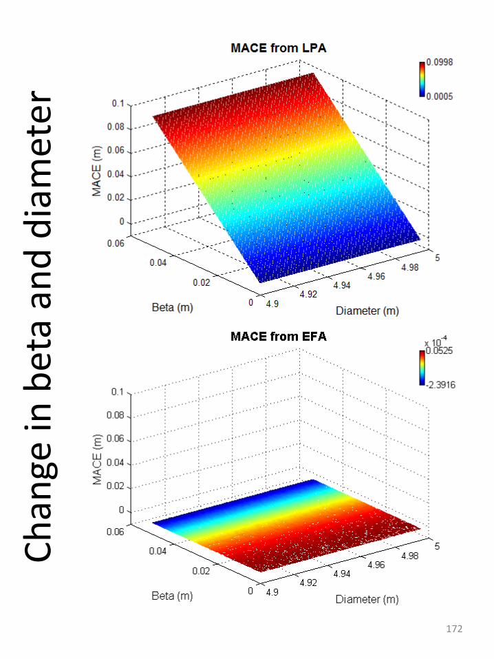
Ch
ange
in b
eta
and
dia
met
er
172
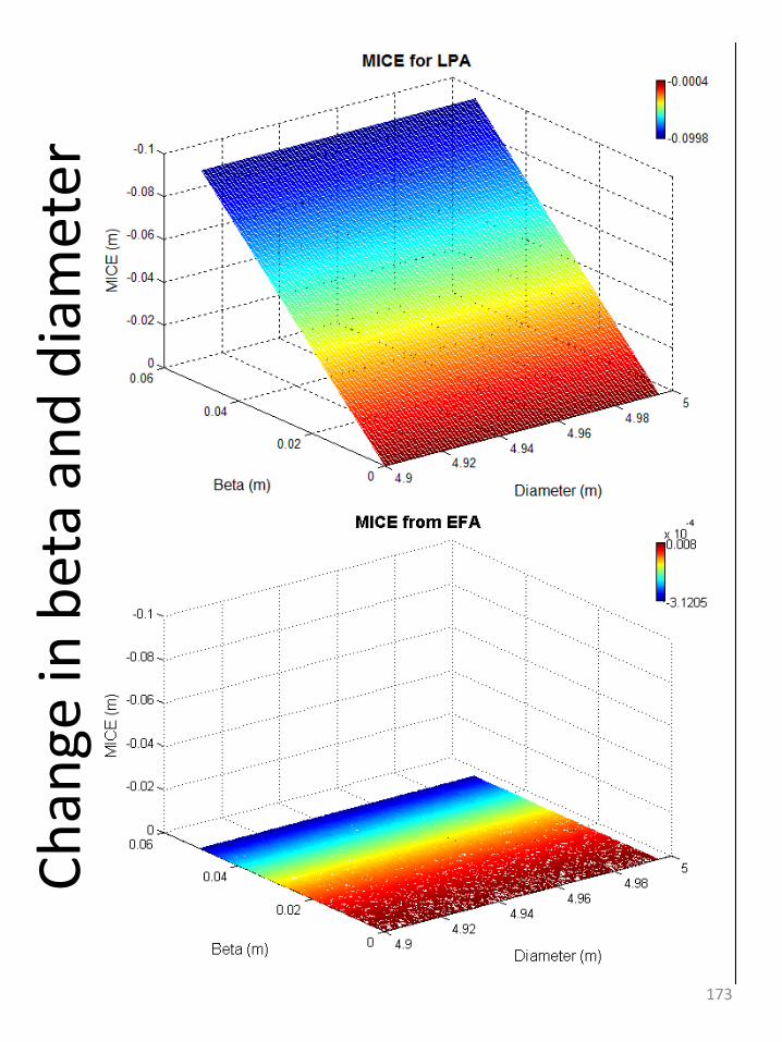
Ch
ange
in b
eta
and
dia
met
er
173
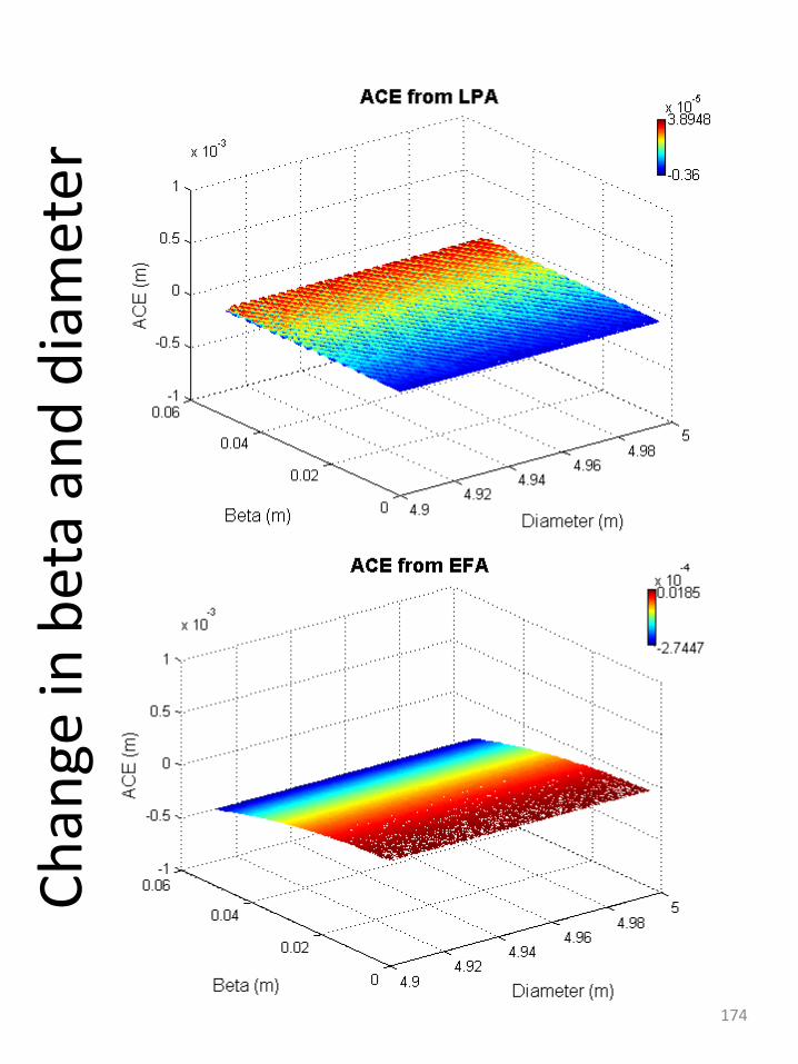
Ch
ange
in b
eta
and
dia
met
er
174
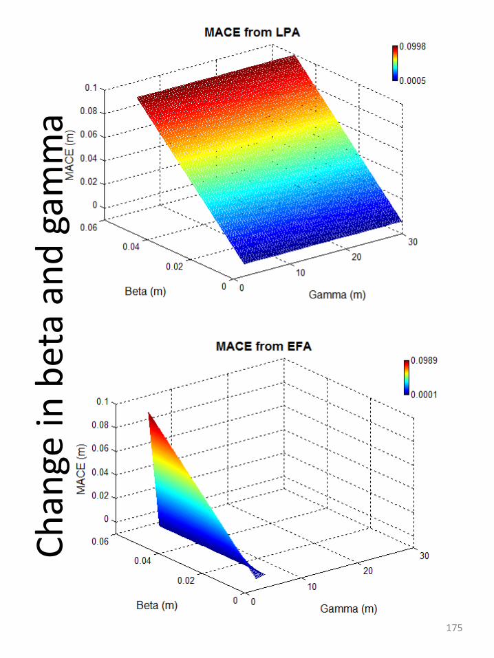
Ch
ange
in b
eta
and
gam
ma
175
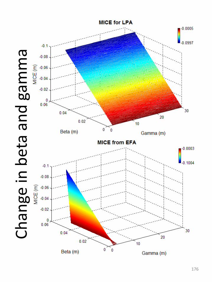
Ch
ange
in b
eta
and
gam
ma
176
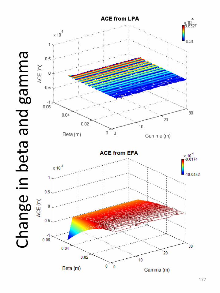
Ch
ange
in b
eta
and
gam
ma
177
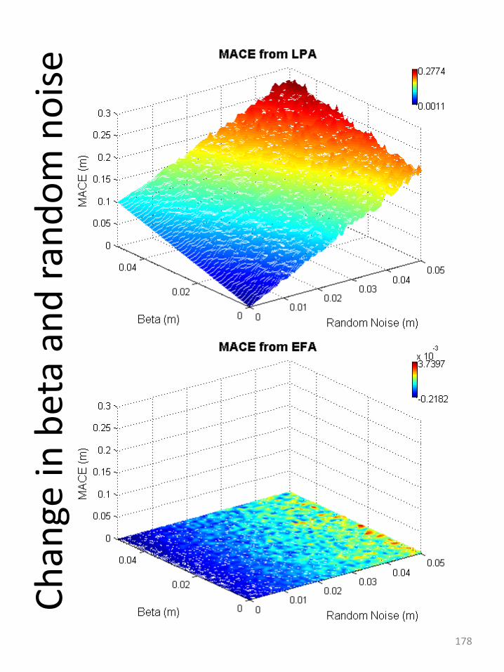
Ch
ange
in b
eta
and
ran
do
m n
ois
e
178
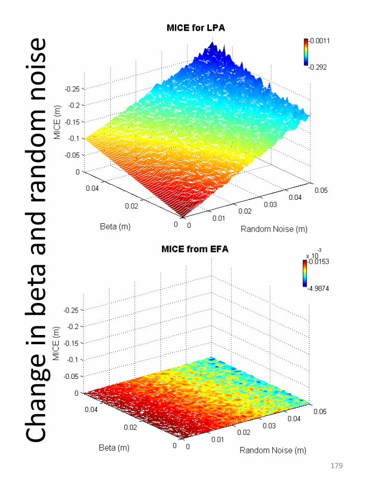
Ch
ange
in b
eta
and
ran
do
m n
ois
e
179
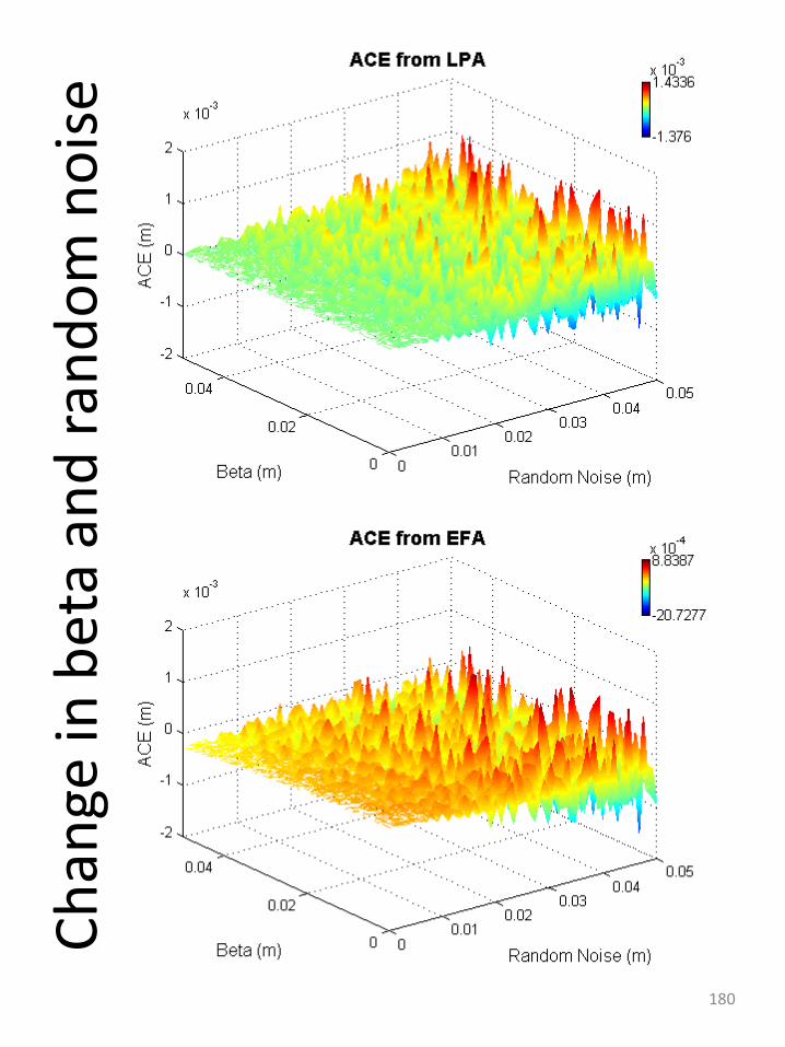
Ch
ange
in b
eta
and
ran
do
m n
ois
e
180
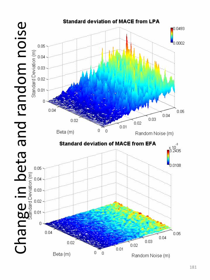
Ch
ange
in b
eta
and
ran
do
m n
ois
e
181
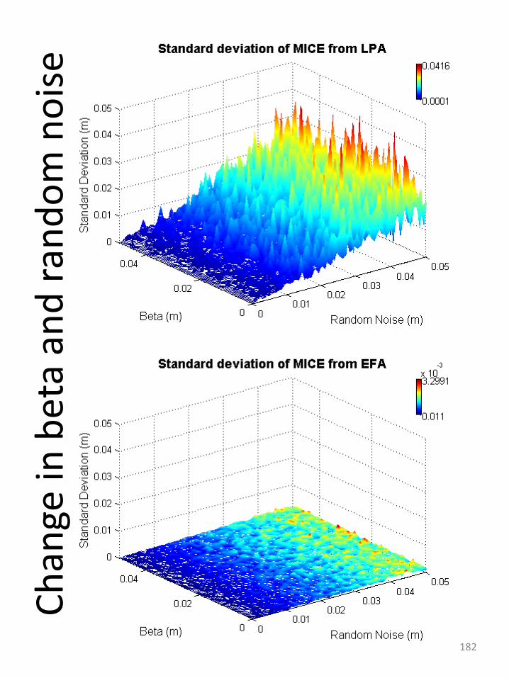
Ch
ange
in b
eta
and
ran
do
m n
ois
e
182
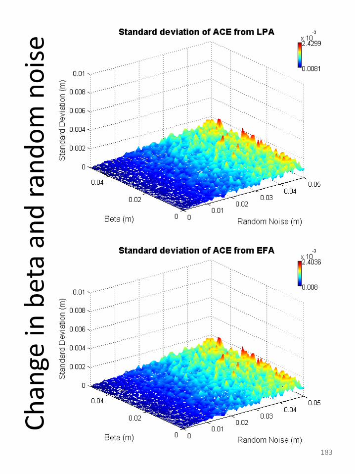
Ch
ange
in b
eta
and
ran
do
m n
ois
e
183
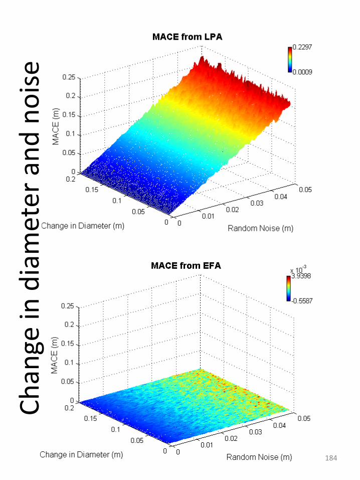
Ch
ange
in d
iam
eter
an
d n
ois
e
184
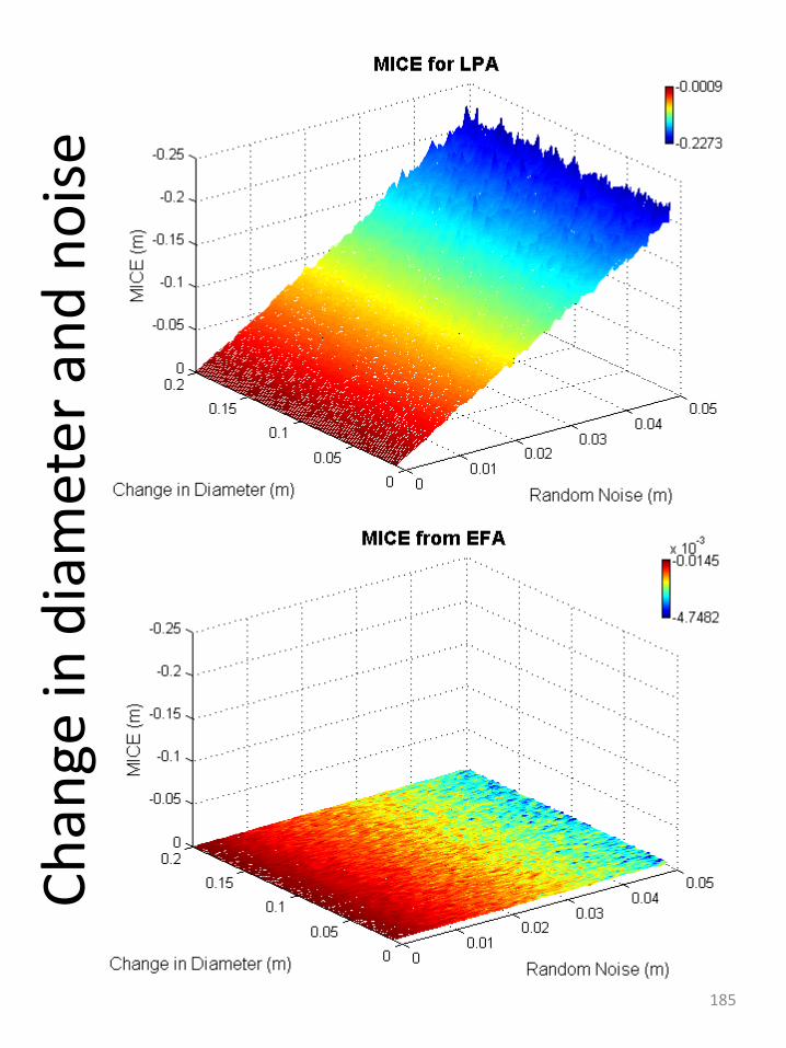
Ch
ange
in d
iam
eter
an
d n
ois
e
185
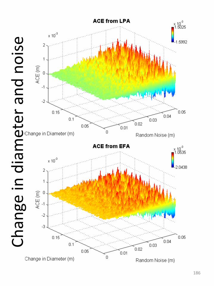
Ch
ange
in d
iam
eter
an
d n
ois
e
186
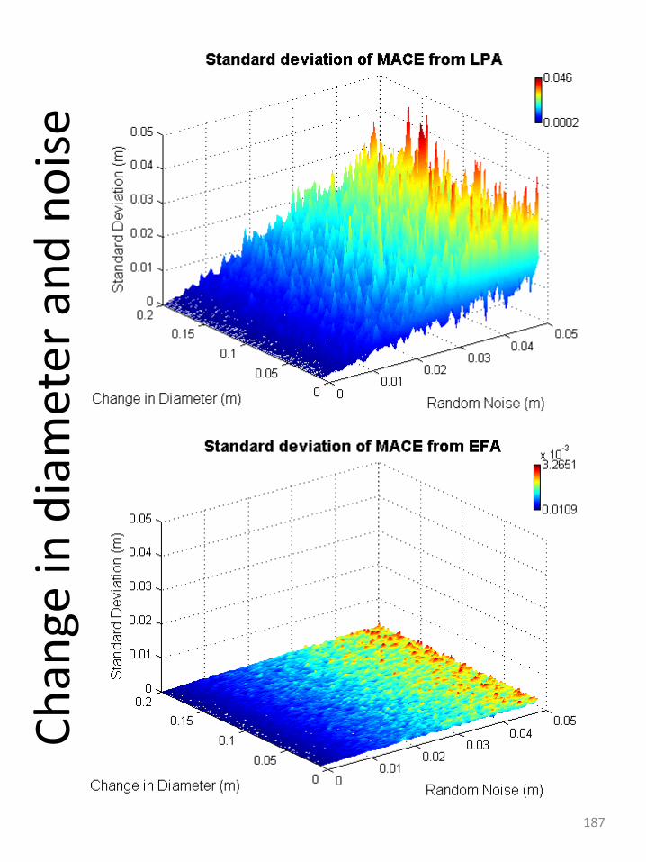
Ch
ange
in d
iam
eter
an
d n
ois
e
187
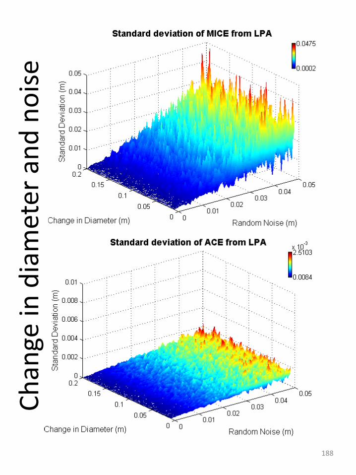
Ch
ange
in d
iam
eter
an
d n
ois
e
188
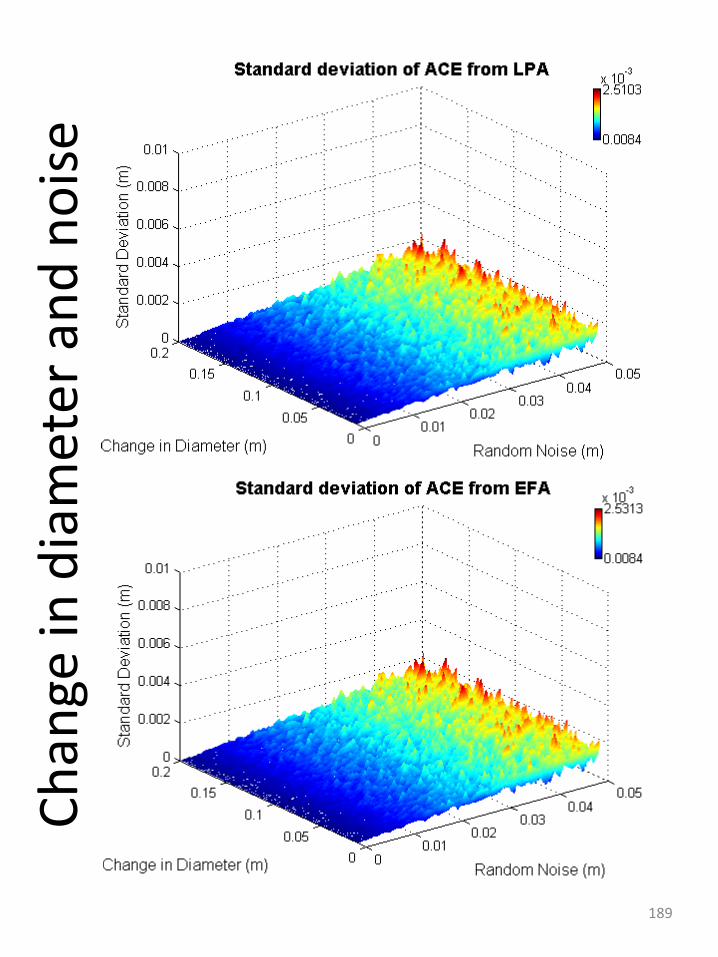
Ch
ange
in d
iam
eter
an
d n
ois
e
189
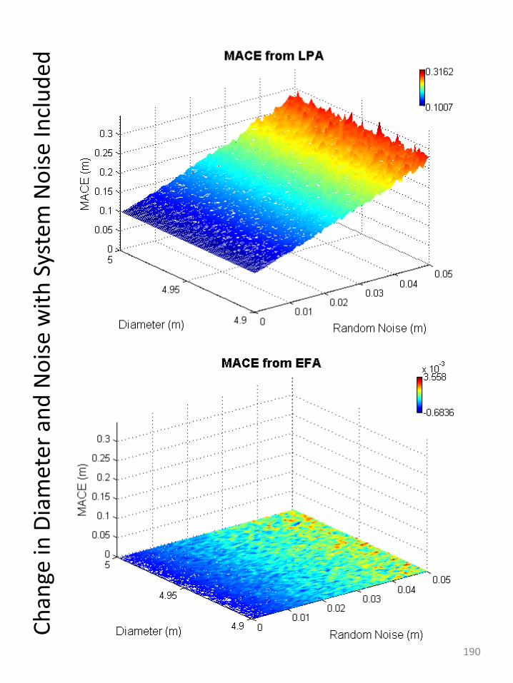
Ch
ange
in D
iam
eter
an
d N
ois
e w
ith
Sys
tem
No
ise
Incl
ud
ed
190
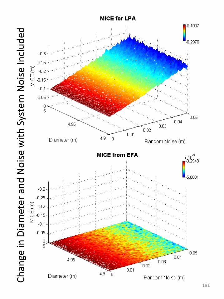
Ch
ange
in D
iam
eter
an
d N
ois
e w
ith
Sys
tem
No
ise
Incl
ud
ed
191
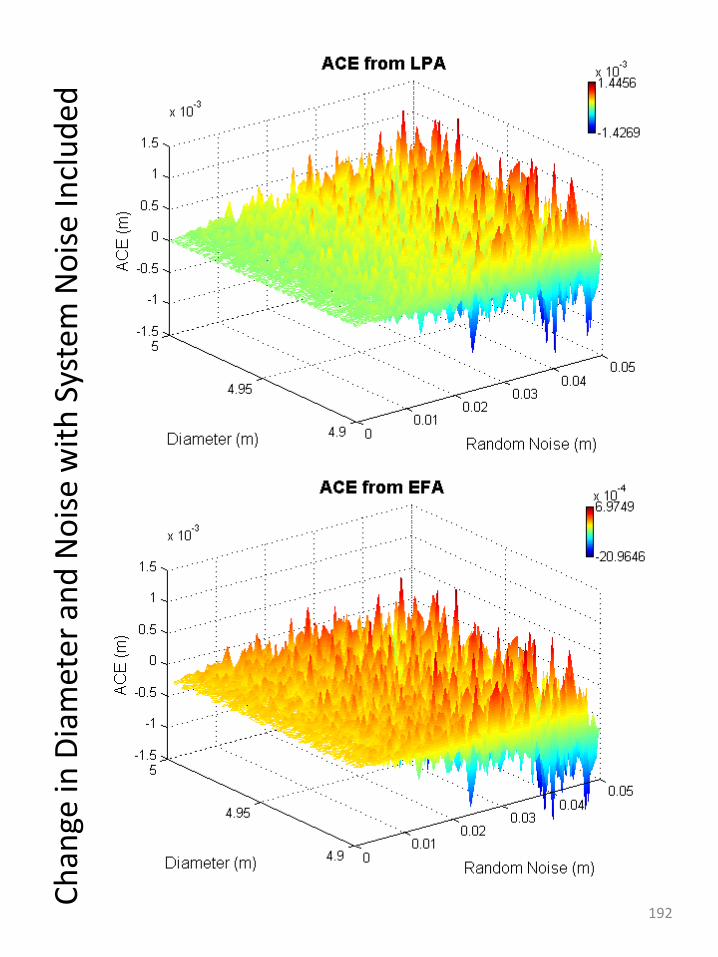
Ch
ange
in D
iam
eter
an
d N
ois
e w
ith
Sys
tem
No
ise
Incl
ud
ed
192
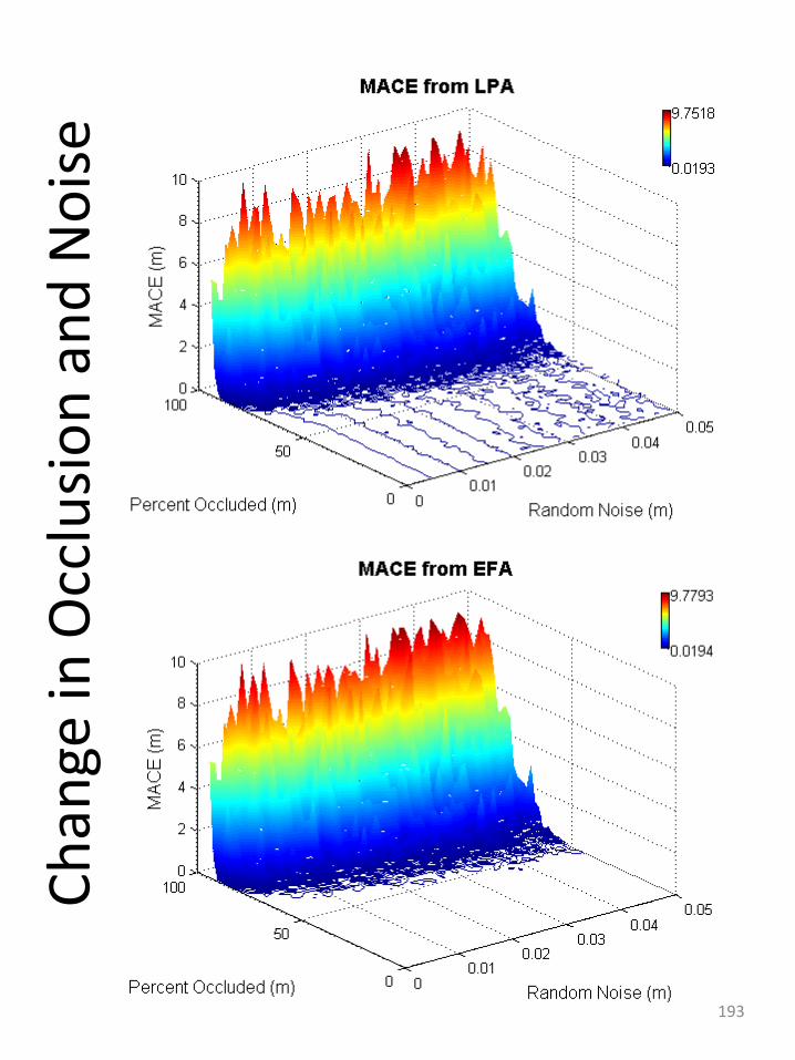
Ch
ange
in O
cclu
sio
n a
nd
No
ise
193
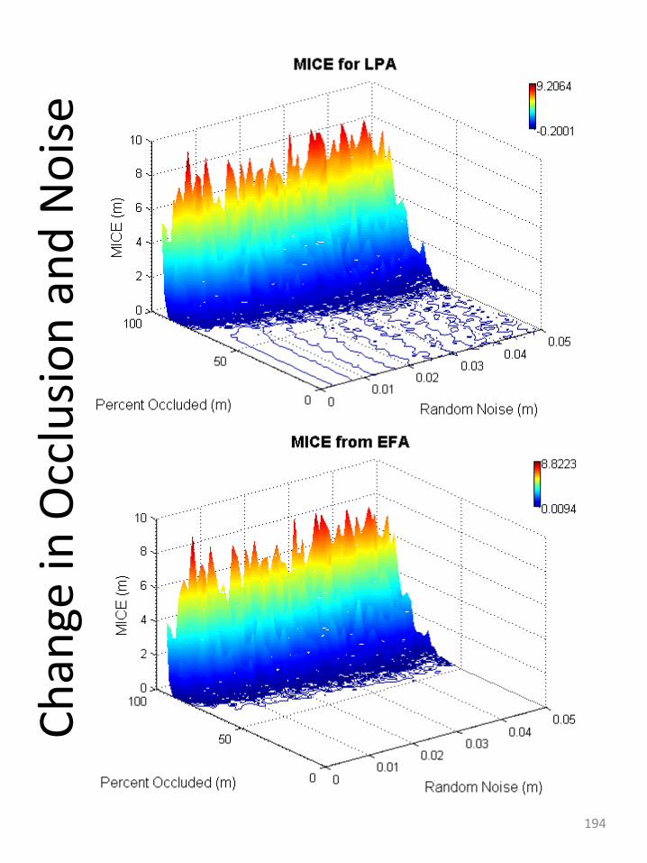
Ch
ange
in O
cclu
sio
n a
nd
No
ise
194
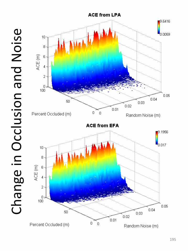
Ch
ange
in O
cclu
sio
n a
nd
No
ise
195
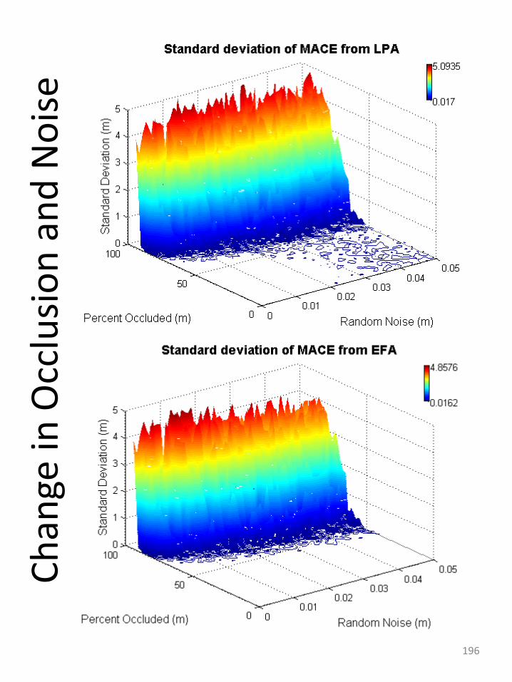
Ch
ange
in O
cclu
sio
n a
nd
No
ise
196
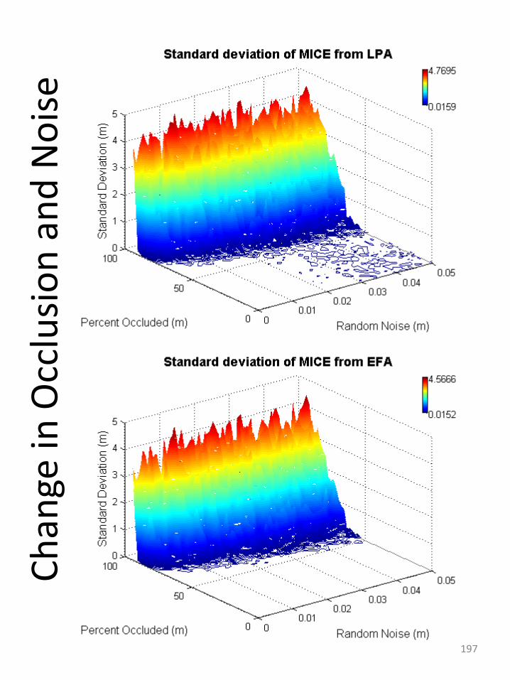
Ch
ange
in O
cclu
sio
n a
nd
No
ise
197
Ch
ange
in O
cclu
sio
n a
nd
No
ise
198
Ch
ange
in N
ois
e an
d S
kew
199
Ch
ange
in N
ois
e an
d S
kew
200
Ch
ange
in N
ois
e an
d S
kew
201
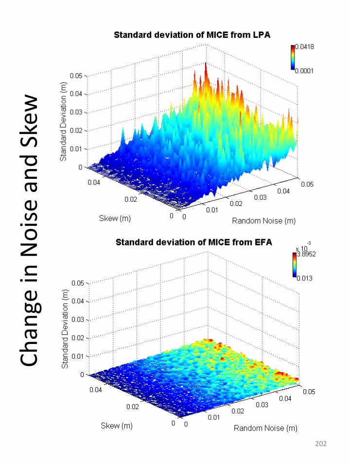
Ch
ange
in N
ois
e an
d S
kew
202