development of a nephelometry camera and humidity
TRANSCRIPT
Portland State University Portland State University
PDXScholar PDXScholar
Dissertations and Theses Dissertations and Theses
1-1-2012
Development of a Nephelometry Camera and Development of a Nephelometry Camera and
Humidity Controlled Cavity Ring-Down Humidity Controlled Cavity Ring-Down
Transmissometer for the Measurement of Aerosol Transmissometer for the Measurement of Aerosol
Optical Properties Optical Properties
James Gregory Radney Portland State University
Follow this and additional works at: https://pdxscholar.library.pdx.edu/open_access_etds
Let us know how access to this document benefits you.
Recommended Citation Recommended Citation Radney, James Gregory, "Development of a Nephelometry Camera and Humidity Controlled Cavity Ring-Down Transmissometer for the Measurement of Aerosol Optical Properties" (2012). Dissertations and Theses. Paper 907. https://doi.org/10.15760/etd.907
This Dissertation is brought to you for free and open access. It has been accepted for inclusion in Dissertations and Theses by an authorized administrator of PDXScholar. Please contact us if we can make this document more accessible: [email protected].
Development of a Nephelometry Camera and Humidity Controlled Cavity Ring-Down
Transmissometer for the Measurement of Aerosol Optical Properties
by
James Gregory Radney
A dissertation submitted in partial fulfillment of the
requirements for the degree of
Doctor of Philosophy
in
Environmental Sciences and Resources: Chemistry
Dissertation Committee:
Dean B. Atkinson, Chair
Reuben Simoyi
James F. Pankow
Linda George
Andrew Rice
Gwynn R. Johnson
Portland State University
©2012

i
Abstract
A Nephelometry camera (NephCam) and Humidity Controlled Cavity Ring-Down
Transmissometer (HC-CRDT) were developed for the determination of aerosol optical
properties. The NephCams use a reciprocal geometry relative to an integrating
nephelometer; a diode laser illuminates a scattering volume orthogonal to a charge
coupled device (CCD). The use of a CCD allows for measurement of aerosol scattering
in 2 dimensions; scattering coefficients and size information can be extracted.
The NephCam's optics were characterized during a set of imaging experiments to
optimize the images collected by the camera. An aperture setting of 1.6 was chosen
because it allowed for the most light intensity to reach the CCD - albeit with significant
vignetting - and also had a constant modular transfer function (MTF) across the image;
approximately 0.3. While this MTF value is approaching the minimum usable MTF of
0.2, other aperture settings did not exhibit constant MTF. While the effects of vignetting
can be corrected in image post processing, the effects of non-constant MTF cannot.
An optical response model was constructed to simulate images collected by the
NephCams as a function of particle type and size. Good agreement between modeled and
measured images was observed after the effects of contrast on image shape were
considered. The image shapes generated by the model also pointed towards the use of
polynomial calibration for particle sizes less than 400 nm as a result of multiple charge-
to-size effects present from the sizing mechanism of the differential mobility analyzer.
Initial calibration of the NephCams using size-selected dry Ammonium sulfate (AS)
showed that calibration slopes are a function of particle size which is also in agreement
ii
with the model. Calibration slopes decreased as particle size increased to 400 nm; after
400 nm calibration slope oscillated around a common value. This effect is directly
related to the forward shift of scattered intensity as particles grow in size and the
collection efficiency of the NephCam as particle size increases. The single scattering
albedo (SSA) of Nigrosin was calculated using the NephCam; extinction was measured
by the HC-CRDT. Good agreement between the SSA and size was noticed for larger
particle sizes; particles smaller than 200 nm in diameter over-measured the SSA of
Nigrosin because of the multiple charge-to-size effect. In this size regime, light
scattering by particles increases much more quickly than absorption; the presence of
larger particles causes scattering to be artificially high.
The HC-CRDT is a 4 channel, 3 wavelength instrument capable of measuring the
extinction coefficients of aerosols at high (> 80%), low (< 10%) and ambient relative
humidity. Extinction coefficients as a function of RH were determined for AS, NaNO3,
NaCl, and Nigrosin; these particles represent surrogates of the strongly scattering ionic
salts and black carbon, respectively. A model was developed to calculate the changes in
refractive index and extinction coefficients of these water soluble particles as a function
of RH; these particle types were chosen because core-shell morphologies could be
avoided. Volume mixing, Maxwell-Garnett and partial molar refraction mixing rules
were used to calculate effective refractive indices as a function of water uptake. Particle
growth was calculated based upon the Kelvin equation.
Measured and modeled results of f(RH) - relative change in extinction between
high or ambient RH and dry RH - agree well for all particle types except Nigrosin. This
disagreement is thought to stem directly from an incomplete parameter set for Nigrosin;

iii
growth parameters were assumed to be identical to NaNO3, density assumed to be 1 g/mL
and molecular weight 202 g/mole, which may not be true in reality (different suppliers of
Nigrosin quote different molecular weights). The NephCam was not used during these
experiments, so the addition of a scattering measurement to better characterize the growth
by Nigrosin is necessary. The f(RH) data for NaNO3 showed excellent agreement
between measured and modeled data; however particle size information collected by an
SMPS does not agree with the theory. This stems from the fact that NaNO3 does not
show prompt deliquescence upon drying; instead an amorphous solid forms which
exhibits a kinetically limited loss of water.

iv
Dedication
For my family...

v
Acknowledgements
"Two roads diverged in a wood, and I --
I took the one less traveled by,
And that has made all the difference."
The Road Less Traveled, Robert Frost (Frost 1916)
Graduate school has been my less traveled road, and it has made all the
difference. This dissertation represents the more than just my work and schooling at
Portland State University, but also quite possibly the greatest adventure of my life. None
of this would have been possible without the many people who helped me follow my own
road.
I owe a special debt of gratitude to my advisor, Dr. Atkinson; it has been a
privilege working in his lab. I couldn't have asked for a better graduate mentor and
colleague.
To my friends, thanks for everything both with graduate school and life. Valerie
Coffey, thanks for being a great friend and roommate. Ashley Sexton, thanks for your
continued support throughout this process. Jon Orleck and Joe Harworth, thanks for all
your help with the development of the instruments here-in and many good times to boot.
Jeremy Parra, thanks for your help with some of the mathematics and the many sanity
checks as we finished our projects and dissertations.
To my family - Mum, Dad and Becky - thanks for your unwavering and unending
moral support and love. I wouldn't be here today without you.
vi
Table of Contents
Section Title Page
-- Abstract i
-- Dedication iv
-- Acknowledgements v
-- List of Tables ix
-- List of Figures x
1. Introduction 1
1.1. Global Climate 1
1.1.1. Greenhouse gases 4
1.1.2. Aerosols 5
1.1.3. Global Climate Models 6
1.2. Focus and questions to answer 7
1.3. Aerosols and climate 7
1.3.1. Direct effects 7
1.3.2. Indirect effects 9
1.3.3. Semi-direct effects 10
1.3.4. Summary of climate effects 10
1.4. Optical properties of aerosols 11
1.4.1. Extinction measurement 11
1.4.2. Theoretical relationship between extinction and size 12
1.4.3. Particles with size near visible wavelengths 15
1.4.4. Scattering phase functions 16
1.4.5. Asymmetry parameter 16
1.4.6. Ångström exponents (α) 17
1.4.7. Single scattering albedo 18
1.5. Particle types and classifications 19
1.5.1. Inorganic particles 19
1.5.2. Carbonaceous aerosols 21
1.5.2.1. BC vs. BrC 21
1.5.3. Primary vs. secondary aerosols 24
1.6. Relative humidity and particles 25
1.6.1. RH and particle thermodynamics 28
1.6.1.1. Kelvin effect 28
1.6.1.2. Köhler effect 31
1.7. Measurement of aerosol optical properties 33
1.7.1. Filter vs. in-situ measurements 33
1.7.2. Single particle vs. bulk measurements 34
vii
1.7.3. Absorption 34
1.7.3.1. Single particle soot photometer 34
1.7.3.2. Photoacoustic spectrometer 35
1.7.4. Scattering 35
1.7.5. Extinction 36
1.8. Present developments and modifications 37
2. Materials and methods 38
2.1. Aerosol generation system for laboratory studies 38
2.2. NephCam 40
2.2.1. Theory of operation 40
2.2.2. Optimization of optical system 42
2.2.3. Physical construction 42
2.2.4. Computer system and data collection 44
2.2.5. Data processing and analysis 45
2.2.6. Scattering coefficients and size information 47
2.3. NephCam size selected experiments 48
2.3.1. "Driftdown" experiments 49
2.4. HC-CRDT 49
2.4.1. Theory of operation 49
2.4.2. Physical construction 51
2.4.3. RH sensors and location 56
2.4.4. Humidifier/Dryer 56
2.4.5. Data processing and analysis 57
2.5. Allan variance 58
2.6. Humidification experiments 58
2.6.1. Flow system setup 58
2.6.2. Aerosols used 60
3. Results and discussion - NephCam experiments 62
3.1. NephCam characterization and getting good images 62
3.1.1. Targets 62
3.1.2. Calibration matrix 65
3.1.3. White background 66
3.1.4. Checkerboard 68
3.1.5. Single line 72
3.2. NephCam size-based calibration experiments 73
3.2.1. 300nm AS 83
3.2.2 100nm AS 93
3.2.3 700nm AS 94
3.3. Calibration slopes as a function of particle size 95

viii
3.4. NephCam summary 102
4. Results and discussion - Humidification experiments 106
4.1. Allan variance 106
4.2. Characterizing direct sums fitting routine 108
4.3. Characterizing HC-CRDT transmission efficiency without
Humidity controls
108
4.4. Humidifier and dryer particle transmission 109
4.5. Measures of particle growth by humidity 112
4.6. Changes in refractive index due to water uptake 116
4.6.1. Water uptake and dilution effects on particle refractive index 117
4.6.1.1. Volume mixing 117
4.6.1.2. Maxwell-Garnett 118
4.6.1.3. Partial molar refraction 119
4.6.2. RF inaccuracies from refractive index changes 120
4.7. Modeling water uptake with RH 123
4.7.1. Inputs 124
4.7.1.1. Refractive index 124
4.7.1.2. Density 124
4.7.1.3. Activity 125
4.7.1.4. Surface tension 126
4.7.1.5. Size distribution data 128
4.7.1.6. RH 128
4.7.2. Assumptions 128
4.7.3. Model overview 130
4.8. AS Results 134
4.9. NaNO3 Results 142
4.9.1. Uncertainty in geometric mean diameter and standard deviation 145
4.10. NaCl Results 153
4.10.1. NaCl γ(RH) 161
4.11. Nigrosin results 163
4.11.1. Calculation of Nigrosin refractive index at other wavelengths 168
5. Conclusions and future directions 173
6. References 177

ix
List of Tables
Table Title Page
1-1 Distinction between carbonaceous aerosols by measurement method 22
3-1 Multiple charge to size particles and fraction for a 300 nm AS aerosol 89
3-2 Multiple charge to size particles and fraction for a 100nm AS aerosol 94
4-1 Allan deviation results as a function of integration time for the HC-
CRDT
107
4-2 Particle transmission ratios 111
4-3 Particle transmission by type 112
4-4 HC-CRDT correction factors 112
4-5 Refractive indices, molecular weights, solid density and ERH/DRH
for modeled species
124
4-6 Modeled density parameters 125
4-7 Modeled activity parameters 125
4-8 Surface tension parameters, molten salt 126
4-9 Surface tension parameters, high concentration limit 127
4-10 Modeled NaCl γ(RH) 162
4-11 Measured NaCl γ(RH) 163
4-12 Nigrosin absorption and refractive index 170

x
List of Figures
Figure Caption Page
1-1 Link between human and earth systems and climatic drivers 2
1-2 Radiative forcings 6
1-3 Extinction, scattering and absorption efficiency for Nigrosin 14
1-4 Extinction efficiency for NaCl 14
1-5 NaCl scattering phase function 16
1-6 NaCl asymmetry parameter 17
1-7 f(RH) by type of aerosol 27
2-1 Aerosol generation system 38
2-2 Radiance Research M903 schematic 41
2-3 NephCam schematic 42
2-4 NephCam block diagram 43
2-5 Hotpixel removal algorithms 46
2-6 Instrumental setup during size-selected experiments. 48
2-7 Conceptual diagram of a cavity ring-down 50
2-8 HC-CRDT schematic 52
2-9 Flow system during humidification experiments. 58
2-10 Flow system during particle transmission experiments 60
3-1 Spherical aberrations 63
3-2 Astigmatism 64
3-3 Actual target 64
3-4 NephCam target 64
3-5 Distortion 65
3-6 Coma 65
3-7 NephCam calibration matrix 66
3-8 Vignetting 67
3-9 NephCam vignetting 68
3-10 Square wave 69
3-11 Ideal contrast 69
3-12 Weak gradient, good contrast 69
3-13 Weak contrast, good gradient 69
3-14 Actual checkerboard 71
3-15 NephCam checkerboard 71
3-16 NephCam single line 72
3-17 NephCam optical response model 75
3-18 300nm AS phase function 83
3-19 Truncated 300nm AS phase function 84
xi
3-20 Scattered light angle of intersection 85
3-21 Cosine weighting 85
3-22 Scattered light transmission intensity by angle 86
3-23 Scattered light transmission intensity by point 86
3-24 Scattered light transmission intensity to CCD by angle 87
3-25 Scattered light transmission intensity to CCD by pixel 88
3-26 300nm AS modeled normalized intensities 88
3-27 300nm AS actual image 89
3-28 300nm AS modeled multiple charge to size effects 90
3-29 300nm AS modeled multiple charge to size effects, normalized 91
3-30 300nm AS modeled multiple charge to size effects, normalized with
MTF
92
3-31 100nm AS modeled multiple charge to size effects, normalized with
MTF
94
3-32 700nm AS modeled multiple charge to size effects, normalized with
MTF
95
3-33 100nm AS calibration curve from model 97
3-34 500nm AS calibration curve from model 97
3-35 100nm AS calibration curve from data 97
3-36 300nm AS calibration curve from data 98
3-37 2nd order model calibration terms by size 98
3-38 2nd order actual calibration terms by size 99
3-39 1st order model calibration terms by size 100
3-40 1st order actual calibration terms by size 100
3-41 NephCam collection efficiency by size 101
3-42 Model calibration intercept by size 101
3-43 Actual calibration intercept by size 101
3-44 Nigrosin SSA by size 102
4-1 Allan variance 107
4-2 Direct sums precision 108
4-3 Particle transmission - no humidifier or dryer 110
4-4 Particle transmission - with dryer 110
4-5 Particle transmission - with humidifier 110
4-6 Nigrosin real effective refractive index 121
4-7 Nigrosin imaginary effective refractive index 121
4-8 Nigrosin extinction by volume fraction 122
4-9 Nigrosin scattering by volume fraction 122
4-10 Nigrosin absorption by volume fraction 123
4-11 Nigrosin SSA by volume fraction 123
4-12 Mole fraction AS vs. % RH 131
xii
4-13 AS particle growth by RH 132
4-14 AS size distribution shifts by RH 133
4-15 AS RH data 135
4-16 AS temperature data 135
4-17 AS visible extinction data 136
4-18 AS geometric mean diameters 137
4-19 AS geometric standard deviations 137
4-20 AS, measured vs. modeled size distributions 138
4-21 AS, visible measured vs. modeled f(RH) 139
4-22 AS, visible measured vs. modeled γ(RH) 140
4-23 AS, UV extinction data 141
4-24 AS, UV measured vs. modeled f(RH) 141
4-25 AS, IR extinction data 142
4-26 AS, IR measured vs. modeled f(RH) 142
4-27 NaNO3 normalized size distributions vs. RH 143
4-28 NaNO3 RH data 144
4-29 NaNO3 temperature data 144
4-30 NaNO3 visible extinction data 145
4-31 NaNO3 geometric mean diameters 146
4-32 NaNO3 geometric standard deviations 146
4-33 NaNO3, measured vs. modeled size distributions 148
4-34 NaNO3, visible measured vs. modeled f(RH) 148
4-35 NaNO3, UV extinction data 152
4-36 NaNO3, UV measured vs. modeled f(RH) 152
4-37 NaNO3, IR extinction data 153
4-38 NaNO3, IR measured vs. modeled f(RH) 153
4-39 NaCl RH data 154
4-40 NaCl temperature data 155
4-41 NaCl visible extinction data 155
4-42 NaCl geometric mean diameters 156
4-43 NaCl geometric standard deviations 156
4-44 NaCl, measured vs. modeled size distributions 158
4-45 NaCl, visible measured vs. modeled f(RH) 159
4-46 NaCl, IR measured vs. modeled f(RH) 160
4-47 NaCl, IR extinction data 160
4-48 NaCl, UV measured vs. modeled f(RH) 161
4-49 NaCl, UV extinction data 161
xiii
4-50 Nigrosin RH data 163
4-51 Nigrosin temperature data 164
4-52 Nigrosin geometric mean diameters 165
4-53 Nigrosin geometric standard deviations 165
4-54 Nigrosin, measured vs. modeled size distributions 166
4-55 Nigrosin visible extinction data 167
4-56 Nigrosin, visible measured vs. modeled f(RH) 168
4-57 Nigrosin absorption spectrum 169
4-58 Nigrosin, UV extinction data 171
4-59 Nigrosin, UV measured vs. modeled f(RH) 171
4-60 Nigrosin, IR extinction data 172
4-61 Nigrosin, IR measured vs. modeled f(RH) 172
1
1. Introduction
1.1. Global Climate
Climate is loosely defined as the average weather of a location over long periods
of time. According to the IPCC 4th Assessment report, climate is the statistical
description of the mean and average variability in surface temperature, precipitation and
wind averaged over months to millions of years (Core Writing Team 2007). Classically,
the climate period has been defined as 30 years by the World Meteorological
Organization (WMO). Climate is generated by interaction between the earth's
atmosphere, biosphere, cryosphere, hydrosphere, and land surface.
Humans have impacted climate ever since the discovery of fire through the
emission of particulate and greenhouse gases. Initially these effects were small relative
to those of the natural system. With the transition from hunter/gatherer societies to
agricultural based societies, humans started to have a larger influence on the planet and
it's climate through the use of fossil fuels and landscape alteration. Post-industrial
revolution, the human effect on climate has increased in magnitude almost exponentially
due to further increases in fossil fuel use; the emission of elevated levels of greenhouse
gases has driven this effect. However, the true magnitude of these effects is still
uncertain.
Interactions between earth and human systems affect the entire planet in many
inter-related ways with even more feedback mechanisms as shown in figure 1-1 (this is as
a vast oversimplification of the problem but serves as a good starting reference).
Emissions of greenhouse gases and aerosol particles by humans have been identified as
climatic process drivers (left box). These drivers affect both the earth system through
climate change (top box) and human systems by affecting socio-economic development

2
(bottom box). Both climate change and socio-economic development are vulnerable
systems that can be impacted (right box). Societies can then respond to both the climatic
drivers and impacts by mitigation and adaptation, respectively.
Figure 1-1: Simplified view of the link between human systems and earth systems and
the effects of climatic drivers on climate and communities. From Contribution of
working groups I, II and III to the fourth assessment report of the intergovernmental
panel on climate change, IPCC, page26, figure I.1 (Core Writing Team 2007).
Climate change can be identified by changes in global mean temperature and
precipitation caused by climatic drivers such as anthropogenic emissions of greenhouse
gases and aerosols. Solar irradiance also plays into climate change, but is outside the

3
realm of human control. These changes are linked to an array of effects: glaciers melting,
sea levels rising, changing ocean circulation patterns, increases in the number of extreme
weather events, etc.
As a result of these climatic changes, ecosystems and resources are impacted and
can become vulnerable and drive further climate change. Societies also become
vulnerable; issues concerning food and water supply, security and human health can
result. When societies become vulnerable, socio-economic development is also
impacted. Societies can then either adapt to or mitigate the climatic changes.
The importance of the research presented here-in is multifold. The occurrence of
global warming and cooling stems from changes in the earth’s radiation budget. When
the amount of solar radiation retained by the planet is larger than the amount re-emitted,
warming occurs. Conversely, when the amount of solar radiation re-emitted by the planet
is larger than the amount absorbed, a cooling occurs. This warming and cooling
represent a delicate interplay between solar irradiance, planetary albedo, greenhouse
gases and aerosols. Changes in the intensity of solar irradiance can drive earth’s climate;
increases/decreases in intensity lead to increases/decreases in planetary temperature,
respectively. However, the relative magnitude of solar irradiance effects over recent
years is minimal as the intensity of the sun has remained relatively constant. Changes in
planetary albedo also affects the radiation budget of the earth; increases in the reflectivity
of the earth’s surface can cause either a warming or cooling influence depending upon the
presence of aerosols aloft. Since a majority of the earth is covered by ocean, which has a
low albedo, the change in surface albedo is minimal relative to other climatic drivers
present like the greenhouse gases and aerosols.

4
The main focus of the work presented here is developing instrumentation for the
better understanding of aerosols. Aerosols mostly oppose the warming influence of
greenhouse gases. However, spatio-temporal variability of aerosols is very high due to
short atmospheric lifetimes (less than 1 week) and the modification of physical and
chemical properties from aging mechanisms. While the instrumentation developed here
is only capable of measuring at a single ground location, it is capable of better
characterizing aerosol optical properties as function of relative humidity. By developing
a better understanding of aerosol optical properties through physical measurement, we are
able to improve the predictions of global climate models (GCM's) through improved
ground truthing.
1.1.1. Greenhouse gases
The warming effects of greenhouse gases have been well documented and are
relatively well understood; it is very likely that the increase in greenhouse gas
concentrations since the industrial revolution are the primary cause of increased planetary
temperatures over what would be predicted with omission of the human influence (Core
Writing Team 2007). Greenhouse gases are comprised of non-reactive and long-lived
gas phase species; CO2, CH4, N2O and halocarbons. The average atmospheric lifetime of
the greenhouse gases is greater than 10 years, so their concentrations are globally
distributed. Greenhouse gases affect climate because they absorb strongly in the IR
wavelengths. Incoming solar radiation at these wavelengths is absorbed, while visible
light is allowed through the atmosphere to warm the planet’s surface. The earth then re-
emits the absorbed visible energy as IR radiation that can be absorbed by greenhouse

5
gases. The earth retains this energy as heat causing the earth to re-radiate this energy as a
slightly warmer black body.
1.1.2. Aerosols
Aerosol particles represent the "wild card" in the radiative budget of the earth and
are not as well understood as any other climatic drivers. This can be seen visually in the
IPCC’s figure on climate change (figure 1-2) in that the total magnitude of the radiative
forcing is approximately that from CO2 but the error bars are approximately that from
aerosol effects. The impact of aerosols can be either a cooling or warming influence
depending ultimately upon the optical properties – scattering and absorption – of the
aerosol and the underlying surface albedo; although cooling is expected to dominate
globally. The optical properties of aerosols can be modified by relative humidity and
atmospheric processing. Further, the lifetime of aerosol particles is short relative to the
greenhouse gases; on the order of minutes to weeks versus years. The end result is that
the radiative affect of aerosols varies strongly both spatially and temporally as a function
of many different parameters.

6
Figure 1-2: Contributions different components to radiative forcing effects. From
Contribution of working groups I, II and III to the fourth assessment report of the
intergovernmental panel on climate change, IPCC, page26, figure I.1 (Core Writing
Team 2007).
1.1.3. Global Climate Models
Many climate models require aerosol chemical and optical properties as input
parameters; model results can vary widely depending upon the exact parameters used
(Bond and Bergstrom 2006). Thus, the improvement of climate models requires a better
understanding of the optical properties of aerosols and their variation both in space and
time as a function of composition. The instruments developed here – a Humidity
Controlled Cavity Ring-Down Transmissometer (HC-CRDT) and Nephelometry Camera
(NephCam) – are both stationary instruments that are either laboratory or field
deployable. While we could gain some information about the temporal evolution of

7
aerosol from these instruments, my focus is on the better understanding of the optics of
aerosol properties as a function of relative humidity.
1.2. Focus and questions to answer
The ultimate focus of my work can be divided into 2 primary components. One
that focuses on the development and characterization of the NephCam as a measurement
and another that focuses on the development of the HC-CRDT and using it to measure
the effects of RH on extinction. My primary research goals are to address the following
questions:
1. Can a CCD be used in place of a PMT as a detector for a better
determination of scattering coefficients?
2. Can image shape be linked to scattering phase functions and ultimately
particle size?
3. What is the effect of relative humidity on the measured optical properties
of aerosol particles?
4. How does the refractive index and size change of the particles as a function
of RH?
5. What is the ultimate effect of RH on the measurements?
1.3. Aerosols and climate
1.3.1. Direct effects
Aerosols affect climate directly through the scattering and absorption of radiation.
The magnitude of these effects is highly dependent on the refractive index and size of the
particles. The refractive index (n) of a material can be represented by
(eq 1-1)
where m and k are the real and imaginary parts, roughly corresponding to the scattering
and absorption efficiency of a material, respectively. Note that n, m, and k are all
functions of wavelength, containing both the classical scattering response and quantum
mechanical connections (i.e., molecular spectra). (A more complete treatment of how
the refractive index, wavelength and scattering and absorption efficiency are related will
8
be presented later.) This allows for a simple classification of aerosol particles into
"white" (k = 0) and "black" (k ≠ 0) types. White particles absorb negligibly in the visible
part of the spectrum but depending upon size can scatter radiation effectively. White
particles are commonly composed of Ionic salts – Na+, NH4
+, Cl
-, NO3
- and SO4
-2 ions –
and non-absorbing organics. Black particles absorb light strongly across the spectrum,
are primarily composed of carbon (elemental carbon) and are formed from combustion
processes. Brown carbon particles absorb light strongly in the ultraviolet but more
weakly in the visible and are also formed in combustion processes. For now, only the
distinction between white and black aerosol (absorbing vs. non-absorbing) will be
considered to elucidate how these aerosols can affect climate. Brown carbon aerosols
will be discussed further in the aerosol optical properties section (Section 2.5.2.1).
Increased loading of white aerosol particles leads to an increase in the reflectivity
of the earth and a cooling or warming effect can result upon the underlying surface
albedo. Increased loading of white aerosols over dark surfaces – low surface albedo –
will result in the "whitehouse effect" (Schwartz 1996); an overall cooling influence due to
an increase in planetary albedo. More solar radiation is reflected back into space. Over
light surfaces like snow and ice – high surface albedo – a warming influence is expected.
Here, solar radiation reflected by the surface can be redirected back towards the planet by
aerosols. The net effect is an increase in the absorption of solar radiation since planetary
reflectance has been decreased by multiple scattering events (Finlayson-Pitts and James
N. Pitts 2000). A majority of earth’s surface (~ 75%) is covered by water which has a
low surface albedo of 0.06 – 0.08 so the cooling influence is expected to dominate
globally (Eck 1987).
9
An increase in the loading of black (strongly absorbing) aerosols leads to an
increase in the absorption of solar radiation. This absorbed light is converted into heat
and re-emitted. The result is warming of the local atmosphere.
The magnitude of the direct optical effects is highly size dependent. Aerosols are
commonly grouped into 3 bins by size: the nucleation, accumulation, and coarse modes:
smaller than 100 nm, between 100 nm and 2.5 µm, and larger than 2.5 µm, respectively.
The nucleation and accumulation modes can be collectively referred to as the fine mode.
As a general trend, scattering and absorption of light by an aerosol increases with size as
a function of particle diameter; (Dp)6 and (Dp)
3, respectively.
1.3.2. Indirect effects
Indirectly, aerosols affect clouds and atmospheric circulation patterns. Aerosols
can act as "seeds" or centers for droplet or ice crystal formation in clouds; a.k.a., cloud
condensation nuclei (CCN) and ice nuclei (IN), respectively. As CCN or IN number
concentration increases, cloud droplet size and precipitation efficiency decrease and
cloud albedo and lifetime increase (Lohmann and Feichter 2005). Atmospheric cooling
or warming can occur as a result of increased reflection of solar or planetary thermal
radiation by clouds, respectively (Schwartz 1996).
The activation of an aerosol particle to become a CCN or IN particle is ultimately
controlled by the composition of the particle and the RH of the air mass in which it is
present. As air rises in the atmosphere, it cools. As a result, the RH of the air mass
increases from the decreased temperature. If temperature decreases enough, the air can
become supersaturated in water vapor.
10
Aerosol particles grow with increasing RH. When water vapor is supersaturated
in air, aerosols can reach a "tipping point" - as predicted by the Köhler equation - at
which the particles will continuously grow as a byproduct of Raoult's law; vapor pressure
of an inhomogeneous liquid is lower than that of the pure liquid. Depending upon aloft
temperature, condensing water can be present in either the liquid or solid phase and the
particle is now considered a CCN or IN particle, respectively.
1.3.3. Semi-direct effects
Strongly absorbing aerosol affects climate semi-directly by changing cloud
formation and atmospheric circulation. Absorption can lead to a local negative climatic
forcing by reducing the amount of radiation reaching earth’s surface: surface dimming.
The local atmosphere becomes warmer, drier and more stable preventing further cloud
formation and water evaporation (Koren, Kaufman et al. 2004). Cloud evaporation is
also possible (Lohmann and Feichter 2005).
1.3.4. Summary of climate effects
While the direct, indirect and semi-direct effects of aerosols on climate have been
well documented, determination of the globally averaged effect remains elusive due to
the spatio-temporal variability of aerosols. Thus the absolute magnitude of each of these
effects is uncertain on global and regional scales. Many climate models require the use
of generalized aerosol data as input parameters, large variation in model results occurs.
Model improvement and uncertainty reduction requires a similar level of improvement
and uncertainty reduction in the measured aerosol optical properties that are used to
refine and ground-truth model predictions.

11
1.4. Optical properties of aerosols
Aerosol particles can either scatter or absorb incident radiation; morphology,
composition and size drives these effects. The sum of scattering and absorption is
referred to as extinction. The exact magnitude of scattering and absorption are a function
of particle refractive index, size and shape. Exact solutions for the optical properties of
any particle can be calculated using Maxwell’s equations, however in many cases the
application of Maxwell’s equations are computationally prohibitive. One of the best
known approximations to Maxwell’s equations is the Lorenz-Debye-Mie Theory (or just
Mie Theory for short). Mie theory includes the constraints that particles are spherically
symmetric and homogeneous. While not all particles in the atmosphere are spherically
symmetric (in reality most are not) Mie theory does provide a good first order
approximation to the optics of all aerosol particles. Other methods, such as the T-Matrix
and discrete dipoles, do exist for the determination of particle optical properties when the
assumptions of particle sphericity and homogeneity are not applicable. However, these
methods are computationally intensive.
1.4.1. Extinction measurement
The removal of light intensity by aerosol particles in the atmosphere, aka
extinction, follows the Beer-Lambert law:
(eq 1-2)
Where I0 is initial intensity, I is the intensity at distance L and bext is the extinction
coefficient. Since both scattering and absorption participate in extinction, the extinction
coefficient can be rewritten as:
(eq 1-3)
12
where babs and bscat are the absorption and scattering coefficients. The extinction,
scattering and absorption coefficients are typically given in units of inverse distance;
inverse megameters (Mm-1
) are our preferred unit, which corresponds to a loss of 1 part
per million of the light per meter of air traversed. For bulk aerosols, the extinction,
scattering and absorption coefficients represent the cumulative contribution from all
particles and sizes present. For a single size bin of particles, the extinction is a function
of the extinction cross-section and the number density of particles:
(eq 1-4)
Where Ni and ζi are the particle number concentration and extinction cross-section of a
particle of size i. The extinction cross-section is a measure of the effective cross-
sectional area a particle has available for interaction with photons. It is not necessarily
the same size as the actual geometric cross-section. Similar relationships exist for the
absorption and scattering coefficients. To derive the extinction coefficient for bulk
aerosols with multiple sizes present, the summation over all particle sizes as a function of
concentration and cross-section is needed:
(eq 1-5)
1.4.2. Theoretical relationship between extinction and size
The extinction efficiency (Qext) of a particle is the ratio of the extinction cross-
section to the geometric cross-section:
(eq 1-6)
Where ζext and ζgeometric are the extinction and geometric cross-sections, respectively. An
identical relationship can be written for scattering and absorption. The geometric cross-
section is related to particle radius through:

13
(eq 1-7)
The size parameter (χ) relates the particle radius to the wavelength of light:
(eq 1-8)
where r is the particle radius and λ is the wavelength of light. Mie theory ultimately
relies on the size parameter for the calculation of optical coefficients. This induces a
scale invariance in the calculation; i.e. nm size particles interact with nm wavelengths the
same as mm size particles with mm wavelengths assuming the different sizes have the
same refractive index at their respective wavelengths.
The extinction, scattering and absorption efficiency of a particle displays 3
regimes relative to particle size as seen in figure 1-3 and 1-4 for a Nigrosin (n = 1.70 +
0.31i) and NaCl (n = 1.55) particle at 532 nm, respectively. In the Rayleigh limit (χ <<
1), the extinction, scattering, and absorption efficiency goes towards 0 as particle size
decreases; the optical effects decrease faster than the particle size; scattering decreases as
r6 and absorption as r
3. In the visible portion of the spectrum, this corresponds to
particles with radii less than approximately 30 nm; roughly the nucleation mode.
In the geometric limit (χ >> 10) the extinction efficiency goes towards 2 as
particle size increases. The absorption and scattering by large particles does increase
with particle size, but does so at a smaller rate. For large particles, absorption shifts from
a volume effect to a surface area effect; it increases as r2
instead of r3. The geometric
limit roughly corresponds to coarse mode aerosols in the visible; particles with radii
larger than approximately 5 μm fall into this category.

14
Figure 1-3: Extinction (solid black), scattering (blue dash) and absorption (red dash dot)
efficiency for Nigrosin (n = 1.70 + 0.31i at 532 nm) particles as a function of diameter.
Figure 1-4: Extinction efficiency for NaCl (n = 1.55 at 532 nm) particles as a function of
diameter.
The Mie paradox is one caveat to the extinction efficiency of coarse mode
aerosols. Under Mie theory, the extinction efficiency approaches 2 as size increases. But
when the same calculations are done using geometric optics instead, the extinction
efficiency approaches 1. This phenomenon is justified because of the shift in scattering
intensity towards the forward direction as particle size increases. Under Mie theory, all
scattered photons are included in the efficiency calculation. Under geometric optics,
photons scattered in the forward direction are not treated as being scattered.
5
4
3
2
1
0
Effic
ien
cy (
Q)
101
2 3 4 5 6 7
102
2 3 4 5 6 7
103
2 3 4 5 6 7
104
Diameter (nm)

15
In the Mie regime (1 < χ < 10), the extinction, scattering and absorption efficiency
hit a maximum; here particle diameter and wavelength are approximately equal.
Interaction of photons and particles increases because of non-linear size effects. The Mie
regime roughly corresponds to the accumulation mode in the visible portion of the solar
spectrum.
1.4.3. Particles with size near visible wavelengths
Solar radiation in the IR and UV wavelengths are strongly absorbed by the
atmosphere. In the vacuum UV (< 200 nm) all radiation is absorbed; molecular O2, H2O,
CO2, N2 and H2 all strongly. In the near-UV, photochemically active species dominate
absorption (O3, O2, CO2, SO2, H2O and Halocarbons) (Horvath 1993). In the IR, the
greenhouse gases dominate (CO2, CH4¸ N2O and Halocarbons) with water vapor also
playing a significant role (Wayne 1996). However, the visible spectrum strongly
transmitted by the atmosphere; NO2 and O3 absorb weakly.
The accumulation mode particles are especially important players in the radiative
balance of the earth because their size is close to the visible wavelengths; light scattering
efficiency reaches maximum as seen in figures 1-3 and 1-4. Accumulation mode
particles also have long atmospheric lifetimes and high number concentrations further
adding to this effect.
Absorption is dominated by fine mode particles, but the nucleation mode particles
play a stronger role than the accumulation mode. Most absorbing particles are
carbonaceous in nature and the result of combustion processes. They are composed of
fractal agglomerates consisting of primary particles with diameters between 20 and 50
nm (Lee, Cole et al. 2002; Mathis, Mohr et al. 2005). Total particle diameters are

16
typically less than 100 nm, but due to their high number concentration play a strong role
in absorption. These particles can be atmospherically processed and grow to
accumulation mode size, but absorption typically decreases relative to the increases in
scattering.
1.4.4. Scattering phase functions
Light scattering as a function of angle by an aerosol can be represented by the
scattering phase function. This represents the normalized plot of intensity as a function
of angle (Integral over all angles equals 1). As particles grow in size, fraction of
scattered light shifts towards the forward direction as evidenced by the 10 nm (black),
100 nm (red), 250 nm (green) and 500 nm (blue) NaCl particle phase functions shown in
figure 1-5. In the Rayleigh limit, scattering is isotropic (equal in forward and backward
directions).
Figure 1-5: Plot of scattering phase function for NaCl particles with diameters of 10 nm
(black), 100 nm (red), 250 nm (green) and 500 nm (blue). Designations of 0° and 180°
represent forward and backward scattering, respectively.
1.4.5. Asymmetry parameter
0
45
90
135
180
225
270
315
10nm 100nm 250nm 500nm

17
The asymmetry parameter (g) represents the intensity weighted average as a
function of scattering angle:
(eq 1-9)
In the limits where g = 1 or g = -1 purely forward or backward scattering is present,
respectively. These limits are never obtained for aerosols. Particles in the Rayleigh limit
can have g values approaching 0 due to isotropic scattering. Particles in the coarse mode
can have g values approaching 1, but 0.9 is a more realistic value. Asymmetry
parameters of an NaCl aerosol as a function of particle diameter can be seen in figure 1-6.
The asymmetry parameter is an important parameter in GCM's; smaller values of g imply
that a larger fraction of scattering is in the backwards direction; an asymmetry parameter
of 0 translates to 50% of scattering being backscatter. Smaller values of g correspond to
a larger fraction of incoming solar radiation being scattered directly back into space or
energy reflected by the planet being scattered back towards earth's surface.
Figure 1-6: Asymmetry parameter (g) of NaCl aerosol as a function of particle diameter.
1.4.6. Ångström exponents (α)
Scattering Ångström exponents (αscat) represent the power law dependence of
scattering on wavelength:
1.0
0.8
0.6
0.4
0.2
0.0
Asym
me
try P
ara
me
ter
(g)
101
2 3 4 5 6 7
102
2 3 4 5 6 7
103
2 3 4 5 6 7
104
Diameter (nm)

18
(eq 1-10)
where bscat,λ is the scattering coefficient at wavelength λ and bscat,λ0 is the scattering
coefficient at a reference wavelength λ0. The differential form of αscat is the more
common form:
(eq 1-11)
Similar equations can be derived for absorption and extinction. The scattering Ångström
exponent is inversely related to particle size; smaller particles have larger values up to a
maximum of 4, while larger particles have values tending toward 0 (Taubman, Marufu et
al. 2004; Bergstrom, Pilewskie et al. 2007; Moosmüller, Chakrabarty et al. 2009).
Absorption Ångström exponents greater than 0 imply the presence of absorbing
material. Black carbon has been shown to have an absorption Ångström exponent near 1
because spectral absorption (governed by the imaginary part of the refractive index k) is
nearly independent of wavelength (Bergstrom, Russell et al. 2002; Schnaiter, Horvath et
al. 2003; Bergstrom, Pilewskie et al. 2007). Other forms of light absorbing carbon, such
as brown carbon and humic-like substances (HULIS), have absorption Ångström
exponents significantly greater than 1; values as high as 6-7 have been reported (Hoffer,
Gelencser et al. 2005; Yang, Howell et al. 2008). This reflects the fact that k only begins
to become significant in the short-wave visible and UV, but then increases dramatically
with decreasing wavelength.
1.4.7. Single scattering albedo
The single scattering albedo (SSA or ω0) represents the fraction of extinction that
is scattering:

19
(eq 1-12)
The SSA is a measure of aerosol "whiteness": for strongly scattering aerosol, ω0 ≈ 1. For
strongly absorbing aerosol it can approach 0 as particle size decreases. The SSA of light
absorbing carbon in the visible is approximately 0.2 (Bergstrom, Pilewskie et al. 2007).
In general, aerosols will be more likely to exert a cooling influence if they have a high
single scattering albedo.
1.5. Particle types and classifications
Aerosol particles exhibit a wide array of chemical compositions that depend upon
both the source and atmospheric processing. The two primary chemical groups or
aerosols are inorganic and carbonaceous particles. However, these two classes are rarely
present as one form or the other but typically as a mixture of both.
Beyond the division of particles into inorganic and carbonaceous; they are also
divided upon formation mechanisms. Primary particles are those particles that are
directly emitted into the atmosphere while secondary particles are formed by chemical
reactions in the atmosphere. Primary particles can be converted into secondary particles
through atmospheric processing.
1.5.1. Inorganic particles
Inorganic particles are typically formed by mechanical processes (primary
aerosol) or gas to liquid condensation or reaction (secondary aerosol). These particles are
primarily composed of the water soluble cations and anions: Na+, NH4
+. K
+, Ca
2+, Mg
2+,
Cl-, NO3
-, and SO4
2-. However, this is not an exhaustive list as a majority of the elements
have been observed depending upon formation mechanism: crustal elements in natural
processes and heavy elements associated with engines and boilers in anthropogenic
20
emissions (Milford and Davidson 1985; Toscano, Moret et al. 2011). The vast majority
of inorganic particles strongly scatter radiation and absorption is minimal. However,
some types of inorganic particles, such as those containing iron oxides (i.e. hematite) and
clay minerals (kaolinite, illite and montmorillonite), can absorb radiation but the total
absorption is small compared to that by carbonaceous aerosols (Finlayson-Pitts and
James N. Pitts 2000).
The lifetime of inorganic particles depends strongly upon formation mechanism.
Mechanically generated particles typically have diameters larger than 3μm and quickly
settle out of the atmosphere. However, sometimes the particles can be re-entrained in the
atmosphere due to surface winds. Saharan dusts have been observed at the Jungfraujoch
site - a free tropospheric site in the Swiss Alps at 3580 m altitude - and in the Caribbean
(Reid, Kinney et al. 2003). Particles produced from gas to liquid condensation or
reaction can have diameters in the accumulation or nucleation range depending upon the
species involved. Lifetimes of these particles are days to weeks depending upon
meteorology; rain tends to scavenge aerosols from the atmosphere.
Many inorganic particles are involatile and relatively inert compared to other
particle types. However, the sulfates and nitrates are not inert and represent a significant
formation pathway for secondary aerosols. SO2(g) can be oxidized to form H2SO4 which
can then further react with or adsorb to particles. NH3(g) can titrate acidic particles; the
NH4+ then remains adsorbed to the particle. Reaction of NH3 with H2SO4 is the primary
production mechanism of ammonium sulfate aerosols. Both of these species are in
relatively high concentrations in the atmosphere due to emission of SO2 from fuels (coal
and diesel) and NH3 from agricultural processes (fertilizers and manure). NO2 can be
21
oxidized to form HNO3 which, like H2SO4, readily reacts with and adsorbs to particles. In
fact, a large number of the oxides of nitrogen have been shown to react with particles
containing chloride and bromide to produce gas phase chlorine and bromine species (De
Haan, Brauers et al. 1999).
1.5.2. Carbonaceous aerosols
Carbonaceous aerosols represents a large class of aerosols that are related on the
basis that they contain carbon. Depending upon composition, morphology and size, these
particles can strongly absorb and/or scatter radiation. They are produced from
anthropogenic and biogenic emissions as both primary and secondary aerosols. Many
naming conventions have been adopted for these particles that can mean similar or
different things depending upon the context.
1.5.2.1. BC vs. BrC
Depending upon the measurement method - thermochemical or optical - similar
classes of carbonaceous aerosols have different names as shown in table 1-1. The total
carbon (TC) content of an aerosol is the sum of all forms of carbon present in the aerosol
minus the contribution from inorganic carbonates. If thermochemical methods are being
employed, TC can be further split into elemental carbon (EC), organic carbon (OC) and
refractory organic carbon. In optical methods, TC is split into black carbon (BC), brown
carbon (BrC) and organic carbon (OC). Both EC and BC are used to describe
carbonaceous aerosols that have properties similar to soot; graphitic layers of carbon
arranged in an sp2 hybridized array. Elemental carbon is typically unreactive – except at
surface sites where reactive species may be present – stable up to very high temperatures
and composed of primary particles that cluster to form fractal like agglomerates. BC
refers to any aerosol with a strong absorption character that is essentially independent of

22
wavelength. Absorption typically shows a λ-1
dependence, i.e., αabs near 1, and mass
absorption coefficient near 10 m2µg
-1 have been observed (Kirchstetter, Novakov et al.
2004; Bond and Bergstrom 2006). Scattering for BC aerosols is usually minimal except
at large particle sizes. While there are not many other components that behave like EC in
terms of the optical properties, it is not guaranteed that a BC aerosol is EC; Nigrosin dye
is a primary example.
Table 1-1: Distinction between carbonaceous aerosols by measurement method (adapted
from (Poschl 2005))
Thermochemical Molecular Structure Optical
Elemental Carbon
(EC)
Graphene Layers (Graphitic
or turbostatic)
Black Carbon
(BC)
Refractory Organic
Carbon
Polycyclic Aromatics,
Conjugated Organics,
HULIS, Biopolymers, etc.
Brown Carbon
(BrC)
Organic Carbon
(OC)
Low Molecular Mass
Hydrocarbons and
Derivatives
Organic Carbon
(OC)
Thermochemically, the OC component of an aerosol is the difference between the
TC and EC. In thermochemical classifications, the temperature dependence and
oxidation reactivity of an aerosol plays a key role in how it is defined. OC consists of
those compounds that are not stable at high temperatures or towards oxidation.
Refractory organic carbon can be misclassified as EC as a result of this temperature and
oxidation stability (Gelencser, Hoffer et al. 2000; Mayol-Bracero, Guyon et al. 2002).
This includes polycyclic aromatics hydrocarbons, Humic-like substances (HULIS), low
molecular weight hydrocarbons, etc.

23
When particle optics are being measured, OC refers to those compounds that have
optical signatures different than BC. This includes colorless organics that do not absorb
or scatter visible radiation like low molecular weight hydrocarbons and their derivatives.
Recently, the classification of brown carbon (BrC) has been added. BrC aerosols do not
absorb appreciably in the visible and NIR, but do absorb strongly in the UV; as a result
BrC particles appear yellow to brown in color. BrC mass absorption efficiencies of 0.031
m2g
-1 at 532 nm and 2-3 m
2g
-1 at 300 nm and αabs as high as 6 - 7 have been reported
(Hoffer, Gelencser et al. 2005). BrC aerosols are commonly composed of polycyclic
aromatic hydrocarbons, HULIS and other polyfunctional groups; the presence of oxygen,
nitrogen, conjugated aromatic systems or multifunctional groups on the aerosol are
thought to drive this enhanced UV absorption (Sun, Biedermann et al. 2007). BrC
possesses a polar character, although it may or may not be water soluble. In fact, the
methanol soluble fraction, versus water or hexane soluble fractions, has been linked to
the increased UV absorption by BrC (Chen and Bond 2009).
BC and BrC are typically the result of combustion processes and originate from
anthropogenic emissions or biomass burning (of which a sizable fraction are still
anthropogenically influenced). The split between BC and BrC depends on combustion
conditions and except for a few distinct cases, such as diesel soot production, a clear link
between conditions and the type of aerosol formed has not yet been elucidated (Andreae
and Gelencser 2006; Chen and Bond 2009). In the case of a diesel engine, BC is formed
in the fuel rich zones inside the piston due to incomplete mixing of fuel and air. This
24
lack of oxygen results in the production of black carbon from the organic backbone, but a
non-negligible organic fraction is also emitted.
Brown carbon possesses significantly more organic carbon character than black
carbon (Chen and Bond 2009). In the case of biomass burning aerosols, BrC emission
has been linked to biomass pyrolysis but actual emissions can vary depending upon fuel
type, amount and conditions (Andreae and Gelencser 2006; Chen and Bond 2009; Levin,
McMeeking et al. 2010). These BrC emissions from biomass burning have come to be
termed Humic-Like Substances (HULIS) for their similarities to Humic acids found in
biomass (Pöschl 2003). BrC has also been shown to be produced from the combustion of
some types of coal, specifically lignite and from the oxidation and polymerization
products of geogenic aerosol (Bond, Bussemer et al. 1999; Andreae and Gelencser 2006).
Because the focus of my dissertation work is on the optical properties of aerosol
and not their thermochemical properties, the terms TC, BC, BrC and OC will be used as
such: TC is the total carbon component present in an aerosol minus that found from
inorganic carbonates. BC represents aerosol components that show optical signatures
similar to that of graphitic carbon; i.e. λ-1
dependence. BrC refers to those aerosol
components that have a stronger wavelength dependence on absorption than BC; i.e.
greater than λ-2
dependence. OC will then refer to any organic components present in an
aerosol that to not optically behave as either BC or BrC.
1.5.3. Primary vs. secondary aerosols
Primary organic aerosols (POA) consist of directly emitted organic aerosols,
semivolatile organic compounds (SVOC) or non-volatile organic compounds (NVOC)
that are condensable under atmospheric conditions. POA is not limited to BrC, but can

25
also include particles generated from wind or traffic-driven re-suspension of organic
particles, biological materials, and sea spray droplets containing organics (Poschl 2005).
Secondary organic aerosols (SOA) are the result of new particle formation from
gas phase or heterogeneous reactions or atmospheric processing of POA. Volatile
organic compounds (VOC's), SVOC's or NVOC's react with oxidant species in the
atmosphere - O3, OH, NOx, Cl and hν to name a few - and results in a many different
product types. Typically, a more oxidized, lower-volatility organic compound (SVOC or
NVOC) is obtained such as carbonyls, carboxylic acids or peroxides. However,
sometimes these products can undergo further oxidation, re-arrangement, isomerization
or decomposition to form more volatile products.
In the event that SVOC or NVOC's are produced by oxidation, these compounds
can then condense onto pre-existing particles or molecular clusters of H2SO4-H2O-NH3 or
form H2SO4-SVOC complexes (Kulmala, Laakso et al. 2004; Zhang, Suh et al. 2004). In
the case of molecular clusters, adsorption or absorption rates of additional SVOC's or
NVOC's is increased as particles grow (Anttila, Kerminen et al. 2004; Kulmala, Laakso
et al. 2004).
1.6. Relative humidity and particles
Relative humidity influences the physical properties of aerosols in a variety of
ways. Water uptake by an aerosol with increasing humidity causes a change in chemical
composition and size; the water content of the particle increases and so must the
diameter. An increase in water content can also trigger a change in particle morphology.
Ultimately, aerosol optical properties are changed as a result of water uptake.

26
Depending upon the type of particle, 3 general classes of aerosol growth as a
function of RH are possible. Aerosols can exhibit hygroscopic growth with hysteresis or
continuous hygroscopic growth or be hygrophobic and exhibit minimal growth as a
function of relative humidity. These growth factors can be represented as hygroscopic
growth factors based upon either particle diameter or optical properties (β(RH) or f(RH),
respectively):
(eq 1-13)
(eq 1-14)
Where D(RH) and D(dry) are the particle diameters at high and low RH, respectively,
and bext(RH) and bext(dry) are the extinction coefficients at high and low RH,
respectively. Similar relationships can be constructed for absorption (fabs(RH)) and
scattering coefficients (fscat(RH)); fscat(RH) is the most commonly used f(RH) form since
scattering tends to be more strongly affected by RH than absorption and extinction tends
to be driven by changes in scattering (Kotchenruther, Hobbs et al. 1999; Andrews,
Sheridan et al. 2004). In both of these equations, the dry RH is taken to be less than 40%,
however this value is not always low enough for a dry measurement of some particle
types (Baltensperger, Barrie et al. 2003). The parameters β(RH) and f(RH) are inherently
linked because the optical properties are dependent upon particle size, but they are not
directly related. As particles take up water, the refractive index of the particle is diluted
towards that of water. This results in the actual f(RH) of a given particle being lower
than expected as defined by β(RH).

27
Strongly hygrophobic particles do not take up appreciable amounts of water and
f(RH) ~ 1 until very high RH, as seen by the blue dot-dash line in Figure 1-7.
Extinction, scattering and absorption are effectively independent of RH for this type.
Many organic aerosols are hygrophobic. When many particles of this class take up water,
a core-shell structure is observed instead of complete mixing within the particle.
Strongly hygroscopic aerosols continuously absorb water at almost all humidities: prime
examples are volcanic ash, H2SO4, NaOH, and soluble organic aerosols (Carrico, Kus et
al. 2003). This is illustrated by the red dashed line in Figure 1-7. Increasing relative
humidity causes these aerosols to grow monotonically (Tang 1976).
Figure 1-7: Plot of f(RH) for hygrophobic aerosol (blue dot-dash), hygroscopic (red
dash) aerosol and hygroscopic aerosol with deliquescence/efflorescence behavior
(black line).
Deliquescent and efflorescent aerosols also take up water from the atmosphere,
but exhibit hysteretic RH dependence. These aerosols can exist as either solid or liquid
particles at the same RH depending on their RH history (which form were they
previously in or which extreme of RH were they last exposed to). Most inorganic salts
exhibit this behavior (Tang 1976). Starting from a low RH – crystalline aerosol – in
28
figure 1-7, these aerosols remain as a crystalline solid until the Deliquescence Relative
Humidity (DRH) is reached. Above the DRH, the aerosol spontaneously absorbs water
and phase transition to a hydrated particle as shown by the upward arrow. As RH
increases beyond the DRH, the aerosol will continue to grow like a hygroscopic aerosol.
From a high RH – starting with hydrated aerosol – the aerosol will remain in a metastable
supersaturated state until the Efflorescent Relative Humidity (ERH) is reached. Below
the ERH, the aerosol spontaneously phase transitions back to a crystalline state, as shown
by the downward arrow. The lifetime of these phase transitions is relatively short, and
has been shown to be less than 10 seconds for sea salt aerosols smaller than 10 μm in
diameter (Lewis and Schwartz 2004). Hysteresis is caused by the fact that ERH < DRH,
sometimes as much as 35% (Freney, Martin et al. 2009).
1.6.1. RH and particle thermodynamics
The effect of water vapor on particle growth is ultimately controlled by physics
but can be described using the Kelvin and Köhler equations. The Kelvin and Köhler
effects are essentially competing terms on particle growth; one (Kelvin) opposes growth
at small particle diameters and the other (Köhler) increases growth at larger particle
diameters. Both equations are based upon the thermodynamics of the aerosol in question.
1.6.1.1. Kelvin effect
The change in free energy of the environment (dGen) containing an aerosol
particle taking up water from the air is the total contribution from both terms:
(eq 1-15)
where dGa and dGw are the changes in free energy of the aerosol and the air (from water
loss), respectively. The change in free energy of the water vapor is a function in the
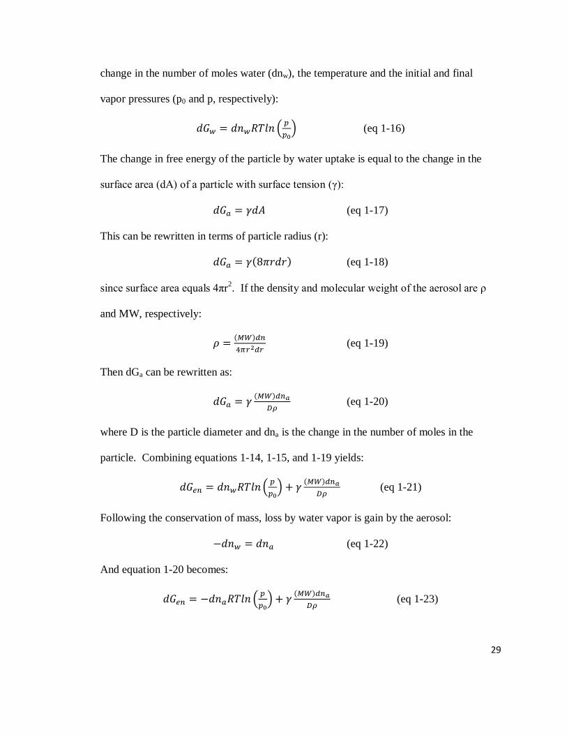
29
change in the number of moles water (dnw), the temperature and the initial and final
vapor pressures (p0 and p, respectively):
(eq 1-16)
The change in free energy of the particle by water uptake is equal to the change in the
surface area (dA) of a particle with surface tension (γ):
(eq 1-17)
This can be rewritten in terms of particle radius (r):
(eq 1-18)
since surface area equals 4πr2. If the density and molecular weight of the aerosol are ρ
and MW, respectively:
(eq 1-19)
Then dGa can be rewritten as:
(eq 1-20)
where D is the particle diameter and dna is the change in the number of moles in the
particle. Combining equations 1-14, 1-15, and 1-19 yields:
(eq 1-21)
Following the conservation of mass, loss by water vapor is gain by the aerosol:
(eq 1-22)
And equation 1-20 becomes:
(eq 1-23)
30
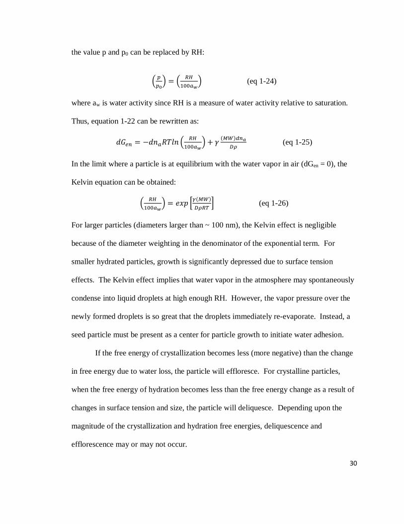
the value p and p0 can be replaced by RH:
(eq 1-24)
where aw is water activity since RH is a measure of water activity relative to saturation.
Thus, equation 1-22 can be rewritten as:
(eq 1-25)
In the limit where a particle is at equilibrium with the water vapor in air (dGen = 0), the
Kelvin equation can be obtained:
(eq 1-26)
For larger particles (diameters larger than ~ 100 nm), the Kelvin effect is negligible
because of the diameter weighting in the denominator of the exponential term. For
smaller hydrated particles, growth is significantly depressed due to surface tension
effects. The Kelvin effect implies that water vapor in the atmosphere may spontaneously
condense into liquid droplets at high enough RH. However, the vapor pressure over the
newly formed droplets is so great that the droplets immediately re-evaporate. Instead, a
seed particle must be present as a center for particle growth to initiate water adhesion.
If the free energy of crystallization becomes less (more negative) than the change
in free energy due to water loss, the particle will effloresce. For crystalline particles,
when the free energy of hydration becomes less than the free energy change as a result of
changes in surface tension and size, the particle will deliquesce. Depending upon the
magnitude of the crystallization and hydration free energies, deliquescence and
efflorescence may or may not occur.

31
1.6.1.2. Köhler effect
The Köhler effect is essentially the opposite of the Kelvin effect. The Kelvin
effect results in a decrease in particle diameter at a given RH due to surface curvature.
The Köhler effect results in activation of an aerosols to form a CCN or IN near or above
supersaturation (RH > 100%). In equation 1-25, if the air is supersaturated with water,
the dGen contribution from water vapor will always be negative. Particles can still grow
to an equilibrium drop size. But, if particle diameter is large enough, then the free energy
contribution by the aerosol will always be less in an absolute sense than the water vapor's
contribution. Thus, dGen will always be negative and will become more negative with
increasing drop size; density and surface tension will become essentially constant due to
droplet size and the composition approaching that of pure water, respectively. When this
occurs, the particle is said to be activated and is now a CCN or IN depending upon
whether water or ice is being taken up by the particle.
Raoult's law also ties into the Köhler effect because it decreases the vapor
pressure of an ideal solution due to other components in the system:
(eq 1-27)
Where pa and pa,0 and xb are the vapor pressure of pure solvent a, vapor pressure a and the
mole fraction of solute b present, respectively. This has the effect of lowering the
supersaturation ratio required for a droplet to become activated and turn into a CCN/IN.
The Köhler effect is the primary driver of cloud formation in the upper
atmosphere. As air masses rise, they cool. This has the effect of increasing the RH of the
air mass to values typically above supersaturation. Many of the particles present in that
air mass can then become activated to CCN or IN because of this increase in RH.
32
The end result of aerosol uptake of any gas phase species is dependent upon the
initial characteristics of the aerosol under investigation. Many water soluble aerosols will
readily uptake water and form a homogeneous mixture. In some instances, surface water
adsorption and structural rearrangement occurs before a hydrated particle is formed; this
effect has been observed in NaCl particles (Krämer, Pöschl et al. 2000; Hämeri,
Laaksonen et al. 2001).
BC and OC aerosols can show different growth properties when gas phase species
condense onto a particle and externally mixed, internally mixed or core-shell particles
result. In externally mixed particles, the carbonaceous particles and the condensing
species are present in separate phases on the same particle. Internally mixed particles
result in a near homogenous particle. With core-shell mixing, the condensing species
forms a shell around the original aerosol which serves as a core. For BC with a fractal
structure, uptake of any coating can induce collapse of the fractal structure (Slowik,
Cross et al. 2007; Zhang, Khalizov et al. 2008).
The core-shell morphology is very common among BC and sparingly soluble OC
when water or H2SO4 condenses onto a particle. The end result is that absorption of light
by the particle is increased due to lensing (Bond, Habib et al. 2006; Bueno, Havey et al.
2011). The exact magnitude of the increase is dependent upon the refractive index of the
coating. Clear coatings such as H2O, H2SO4 or clear OC result in a much larger increase
in absorption than absorbing coatings such as BrC (Lack and Cappa 2010). Absorption
increase is inversely related to the absorption strength of the coating. Regardless of what
type of coating is present, the increase in particle size results in an increase in light
scattering by the particle.
33
Coating thickness dictates the extent to which absorption increases. For small
particles, any coating will increase absorption, but thicker coatings result in larger
absorption increases. For cores larger than about 150 nm, absorption increase is
essentially constant regardless of shell size (Bond, Habib et al. 2006). The same trends
are true for absorbing coatings, but the extent of increase is smaller (Lack and Cappa
2010).
1.7. Measurement aerosol optical properties
Many measurement techniques exist for the determination of aerosol optical
properties. These techniques are categorically divided between filter versus in-situ
measurements and single particle versus bulk measurements. All sub-categories have
their own inherent advantages and disadvantages. These sub-categories can be further
split depending upon the property under investigation: extinction, scattering or
absorption.
1.7.1. Filter vs. in-situ measurements
Filter measurements of aerosol optical properties require the deposition of
particles onto a membrane or fiber filter for measurement, whereas in-situ measurements
measure the optical properties of the aerosol as it flows through the instrument. Filter
measurements are easily implemented and relatively inexpensive compared to many of
the in-situ measurements. Filter measurements can also offer greater spectral coverage
then their in-situ counterparts; the Aethalometer operates at 7 wavelengths across the
solar spectrum.
Depending upon the exact filter characteristics and type, overestimation of
absorption coefficients can occur due to multiple scattering effects by the filter and

34
deposited particles. Typically, whenever more than a monolayer of particles is deposited
on the filter, a correction must be made and can be significant (Campbell, Copeland et al.
1995). Further, particle collection on a filter can alter particle morphology; BrC particles
have been observed to form beads on filter fibers instead of maintain their natural shape
like BC particles (Subramanian, Roden et al. 2007). It is also possible for volatile
compounds to evaporate off of the filter surface during collection resulting in an
incomplete measurement of particles present (Subramanian, Roden et al. 2007).
1.7.2. Single particle vs. bulk measurements
In-situ measurements operate by passing particles through a flow tube or cell
where a measurement of particle optics can be made. Many different types of in-situ
measurements exist, and they are commonly split between whether a single particle or
bulk measurement is being made. The single particle measurements can provide
significant amounts of information about the particle under investigation but can miss
much of the information contained within bulk aerosol. The reverse is true of bulk
measurements in that less information about specific particles is collected, but ensemble
effects are quantifiable.
1.7.3. Absorption
1.7.3.1. Single particle soot photometer
Laser induced incandescence (LII) can characterize thermally refractory particles
such as elemental carbon. LII does not do well with organic carbon or non-absorbing
particles due to a lack of thermal incandescence. In LII, a particle is heated to its boiling
point by an intense laser and subsequently incandesces. The total amount of
incandescence is proportional to the mass of elemental carbon present. While LII is
based upon particle absorption, LII does directly measure absorption; incandescence is a

35
function of mass. With an approximation of the mass absorption coefficient, absorption
coefficients can be obtained. The Single-Particle Soot Photometer (SP2) is a
commercially available instrument based upon the LII technique. The SP2 is also
equipped with multiple photodectors allowing for the determination of light scattering
from which particle size can be inferred.
1.7.3.2. Photoacoustic Spectrometer
The photo-acoustic spectrometer (PAS) is capable of directly measuring
absorption coefficients by aerosol particles. Unlike the SP2, the PAS measures the bulk
absorption coefficient. It operates on a similar principle to the SP2, but has some
fundamental differences. A pulsed laser is used to heat an aerosol sample. Upon
absorption, the particles will transfer heat to the surrounding air and a pressure (sound)
wave is created that can be detected by a microphone. The PAS suffers from non-
idealities in mass transfer effects by the particle. If surface coatings, such as water or
volatile organics, are present on the surface of an absorbing aerosol, these coatings can be
evaporated when the particle is heated. This results in less of a pressure wave being
emitted by the particle and an under-measurement of the absorption coefficient.
1.7.4. Scattering
Light scattering by aerosols is commonly measured by a Nephelometer; the
integrating and polar nephelometer are the most common. In an integrating
nephelometer, a flash lamp illuminates a scattering volume containing aerosol particles.
The light scattered by the particles is then directed to a photomultiplier tube through a
series of baffles. The amount of light reaching the PMT is directly proportional to the
total scattering by the aerosol particles. Integrating nephelometers suffer from truncation
angle effects; the total range of collected scattering is less than the ideal 0° to 180°. As
36
particle size increases, the truncation angle effect worsens because scattering shifts more
toward the forward direction.
Polar nephelometers operate by illuminating a scattering volume using a laser
beam. The light scattered by the particles is then measured by multiple photo-detectors
placed at various angles between 0° and 180°. Polar nephelometers offer a couple
distinct advantages over integrating nephelometers. Size effects can be corrected,
because scattering intensity is collected as a function of angle. The elucidation of
scattering phase function and asymmetry parameter is also possible from this angular
information.
1.7.5. Extinction
Many measurements for extinction by aerosol particles exist, but the single-pass
cell, multi-pass cell and cavity ring-down spectroscopy are the most common. In a
single-pass or multi-pass extinction cell, light is directed into a large flow cell typically
larger than 100 L and longer than 20 m in size. The extinction by aerosols is then
measured by comparing the difference in light transmission through the cell when
aerosols are present and absent. The single and multi-pass cells suffer from high limits of
detection (typically greater than 20 Mm-1
) and physical size constraints.
To improve on the detection limits and sensitivity of the single and multi-pass
cells, cavity ring-down (CRD) has been implemented for the measurement of extinction
coefficients. A laser pulse is directed into an optical cavity consisting of a pair of highly
reflective mirrors. As the laser pulse traverse the cavity, light intensity decays
exponentially due to absorption and scattering by aerosols, the mirrors and any gases
37
present in the cavity. Extinction coefficients are obtained by taking the difference
between decay constants when aerosols are present and absent.
1.8. Present developments & modifications
Presently, a nephelometry camera (NephCam) and a humidity-controlled cavity
ring-down transmissometer (HC-CRDT) have been developed for the determination of
scattering and extinction coefficients, respectively, of aerosols. The NephCam is
different than either an integrating or polar nephelometer in that it uses a charge coupled
device (CCD) to measure the intensity of light scattered by aerosols instead of a PMT.
Like other nephelometers, the NephCam suffers from truncation angle effects, however
because area based detection is being used (by virtue of the CCD), these effects can be
corrected. A model simulating the physical construction of the NephCam was developed
for the comparison of actual image shapes to modeled image shapes to test agreement
between reality and theory.
The HC-CRDT is a 4 channel CRD that is capable of measuring the extinction
coefficients of aerosols at 3 wavelengths (355 nm, 532 nm, and 1064 nm) at high (>
80%), low (< 10%) and ambient humidity simultaneously. This type of instrumental
setup allows for the determination of humidity effects on the optics of aerosol particles in
real time. A model to link the observed changes in extinction to theory was developed
for comparison.
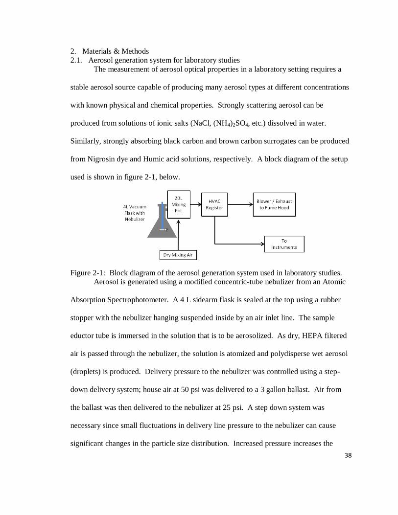
38
2. Materials & Methods
2.1. Aerosol generation system for laboratory studies
The measurement of aerosol optical properties in a laboratory setting requires a
stable aerosol source capable of producing many aerosol types at different concentrations
with known physical and chemical properties. Strongly scattering aerosol can be
produced from solutions of ionic salts (NaCl, (NH4)2SO4, etc.) dissolved in water.
Similarly, strongly absorbing black carbon and brown carbon surrogates can be produced
from Nigrosin dye and Humic acid solutions, respectively. A block diagram of the setup
used is shown in figure 2-1, below.
Figure 2-1: Block diagram of the aerosol generation system used in laboratory studies.
Aerosol is generated using a modified concentric-tube nebulizer from an Atomic
Absorption Spectrophotometer. A 4 L sidearm flask is sealed at the top using a rubber
stopper with the nebulizer hanging suspended inside by an air inlet line. The sample
eductor tube is immersed in the solution that is to be aerosolized. As dry, HEPA filtered
air is passed through the nebulizer, the solution is atomized and polydisperse wet aerosol
(droplets) is produced. Delivery pressure to the nebulizer was controlled using a step-
down delivery system; house air at 50 psi was delivered to a 3 gallon ballast. Air from
the ballast was then delivered to the nebulizer at 25 psi. A step down system was
necessary since small fluctuations in delivery line pressure to the nebulizer can cause
significant changes in the particle size distribution. Increased pressure increases the
39
aerosol number concentration, but decreases geometric mean size of the droplets and thus
the dried particles. Increasing solute concentration in the aerosol solution results in an
increase in both aerosol number concentration and geometric mean size. A major
advantage of this strategy is that the copious amount of water droplets that are produced
by the nebulizer get recaptured and recycled within the flask, so the solutions can be used
continuously for days.
The flask used in the aerosol generation is connected directly to a 20 L aluminum
pot (turkey deep fryer) using a short (~ 1") piece of rubber tubing that seals the sidearm
outlet to a hole in the side of the pot. HEPA filtered dilution air at 30 Lpm enters the
mixing pot from the opposite side of the aerosol stream. This results in a swirling air
pattern within the mixing pot that encourages mixing and drying of the aerosol droplets.
The perforated poultry rack (from the turkey deep fryer) is inverted so that aerosol must
pass upwards through the holes in the rack to enter the 4" PVC exit tube, ensuring that
the aerosol is well mixed before leaving the mixing pot. During size-selected
experiments, the dilution air stream is dried by passing it through a silica gel dryer.
During the non-size selected experiments, the RH of the dilution air was controlled by
splitting the dilution air and passing it through a silica gel dryer to lower RH and/or a
bubbler to increase RH. By controlling the flow rates through each side of the split, the
ambient RH could be raised or lowered from near 50% to less than 10% depending upon
ambient temperature.
Aerosol exits the mixing pot through a 4" O.D. piece of PVC pipe connected to a
4" O.D. aluminum HVAC duct for transport to a modified and combined pair of
Aluminum registers that form a 4" x 4" x 8" box with diagonal inlet and outlets. In the
40
non-size selected experiments, an aerosol cyclone (URG 2000-30EQ, Teflon coated
aluminum cyclones with a nominal 1.0 µm cutoff at 6 Lpm flow) is placed in this box
and connected to 1/2" Cu tubing for transport to the instruments using modified wide-
bore Swagelok fittings. For the size-selected experiments, only the 1/2" Cu tubing is
present as aerosols are directly transported to the DMA(the DMA has a 1.0 μm impactor
so the cyclone was not necessary). The register box sits in line with the Aluminum
HVAC tube and a squirrel cage blower that controls the aerosol flow and exhaust to the
fume hood.
2.2. NephCam
2.2.1. Theory of operation
Bulk aerosol scattering coefficients are commonly measured using a
nephelometer. In a traditional integrating nephelometer, such as the Radiance Research
M903 (figure 2-2) a flash lamp is pulsed inside of a sample chamber, illuminating aerosol
particles with broadband incoherent light. Scattered light is directed through a series of
baffles and a bandpass filter (not shown) to a photomultiplier. The baffles are arranged
so that the light scattered toward the photomultiplier is almost directly proportional to the
scattering coefficient. This type of integrating nephelometer suffers from truncation
errors that cause negative bias in the measurement of the aerosol scattering coefficient for
larger particles.

41
Figure 2-2: Schematic of a Radiance Research M903 integrating nephelometer.
The Radiance Research M903 integrating nephelometer is particularly prone to
truncation errors. Because of the instrument orientation, the PMT can only collect light
scattered between 10°and 170° relative to the direction of light propagation
(Heintzenberg, Wiedensohler et al. 2006). As aerosols grow in size, the scattering
intensity shifts towards the forward direction (0° - along the original light path); the
fraction of light not detected by the PMT will also increase as the aerosols grow in size,
and total scattered light intensity is under-measured. This truncation error by the
Radiance Research nephelometer has been shown to grow monotonically with aerosol
size and be about 5% for 200 nm aerosol and 23% for 1 μm geometric mean diameter
aerosol (Müller, Nowak et al. 2009).
The nephelometer that is incorporated into our instrument uses a different
strategy, based on the reciprocal geometry. Digital charge coupled device (CCD)
cameras are positioned orthogonally to an incident laser beam, as shown in figure 2-3.
As an aerosol passes through the laser beam, light is scattered upwards towards the
camera after being focused by multiple lenses. Unlike photomultipliers, CCDs are area
sensitive detectors allowing a 2-dimensional representation of the aerosol scattering
intensity AND thus a spatial distribution.

42
Figure 2-3: Schematic of NephCam.
2.2.2. Optimization of optical system
A green LED light box was created for optimization of the NephCam's physical
setup. Green LED's were chosen to mimic the green diode laser used during
experimentation. Images of different types of calibration images were taken to
investigate the presence and effects of image distortions: targets for astigmatism, dot
matrices for coma and distortion, a white background for vignetting and a checkerboard
for contrast and Modular Transfer Functions (MTF's). The aperture settings were
optimized to obtain the best possible contrast and image quality. Images at aperture
settings of f = 1.6, 4 and 8 were collected.
2.2.3. Physical Construction
In theory, the scattering of a bulk aerosol could be measured by placing a detector
at a 90° angle in a CRD experiment. In practice, the pulsed laser does not provide
enough intensity to measure scattering. However, a continuous laser source can be used
to generate enough scattered laser power to be measurable. We designed and built a new
type of scattering instrument that we call nephelometry cameras (NephCams) that use a
CCD detector to measure aerosol light scattering. This scattering measurement is
complementary to the extinction measurement produced by the HC-CRDT. A schematic
diagram of the NephCams can be seen in figure 2-4.

43
Figure 2-4: Block diagram of the NephCam aerosol scattering instrument.
Images of light scattering by aerosols are taken using one CCD camera (ThorLabs
DCU224M USB – 1.3 MPixel monochrome CCD, 1280x1024 pixels) per channel. The
NephCam instrument body was constructed from a 6" x 4" x 1.5" (L x W x H) aluminum
block. Two 1/2" Al rods and a 90-degree rod mount were used to form a rigid scaffold
which was affixed to the NephCam body using JB–Weld to serve as a camera mounting
arm. The camera is aligned orthogonally above the aerosol flow and laser beam.
Cameras are aligned such that laser beam propagates along the long (x-axis) such that
image pixels 0 and 1279 are forward and backward, respectively. NephCams view light
scattering through a 1.0" glass window.
44
A green laser diode (Information Unlimited LM532-20, 20 mW, λ = 532 nm) was
mounted in an Al mount using thermally conductive epoxy (Arctic Silver). This laser
mount was attached to the camera mount using a 1" section of straight copper tubing to
ensure proper alignment. The laser beam passes through a 7/16" diameter hole cut
through the length of the NephCam body (as shown in figure 2-4, Top View). A single
laser baffle is present before the laser enters the scattering volume to reduce diffractional
spreading. Without the inclusion of a laser baffle, diffractional spreading leads to
significant wall scattering interference. Laser light that is not scattered is optically
removed using a beam dump at the far end of the camera mount.
Aerosol flow propagates through a 1" hole cut corner to corner of the Al block
and crosses the laser beam axis at an acute (~ 16°) angle. Light scattering takes place in
the center of the flow axis, minimizing wall interference. Two 1/2" to 3/4" Cu pipe
unions provide the step up/down from the 1" aerosol flow channel to 1/2" sections of
straight Cu pipe. The 1/2" straight pipe is then further reduced to 1/2" Cu tube using
Swagelok fittings. This 1/2" Cu tube connects the NephCams to the valving system and
input of the HC-CRDT. Scattering images are focused onto the CCD using a plano-
convex lens (ThorLabs, focal length = 25.4 mm, diameter = 1") and a CCTV lens system
(Tamaron MVL25, focal length = 0.25 m, aperture = 1.6).
2.2.4. Computer system and data collection
Data collection for all 4 cameras was controlled using LabView 8.6 vi's and the
uc480 drivers supplied by ThorLabs. Prior to data collection, all cameras were initialized
to use a digital trigger, 10 second exposure length, and a master gain of 1. Image settings
45
were initialized to a Y8 Monochrome color scheme (8-bit, black and white) and an image
size of 1280 by 1024 pixels (full sensor area).
Semaphore control of the ThorLabs uc480 drivers and image buffer required that
image triggering and transfer be done sequentially for each channel. Image collection
was initiated by a digital trigger that takes approximately 10 msec to complete. After
image exposure, image data was read from the camera to the uc480 buffer; approximately
25 msec. Immediately after transfer the image data was written into an IMAQ buffer in
LabView so that the uc480 buffer could be reused for other channels. Because of this
semaphore control scheme, the camera triggering and data transfer processes were spaced
50 msec apart between channels to ensure that both processes had enough time to
complete with extra overhead in case of computer lag.
Images collected by the cameras were stored directly as .jpeg files with no
compression. The images are converted to data arrays during the analysis. Time stamps,
image number and valve state of the HC-CRDT were written to a separate Excel comma
separated values (.CSV) file. Valve states were read from the PXI box on the HC-CRDT
computer using a local area network connection.
2.2.5. Data processing and analysis
Raw images taken by the NephCams require significant processing for the
extraction of aerosol size and aerosol scattering coefficients. As with the HC-CRDT, the
NephCams require that the difference between clean and aerosol laden air be calculated
to determine aerosol contribution. From the resulting difference images, information
about aerosol size and aerosol scattering coefficients can be extracted by using image
information along the horizontal and vertical axes, respectively. While this background
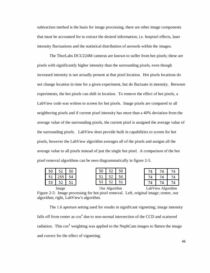
46
subtraction method is the basis for image processing, there are other image components
that must be accounted for to extract the desired information; i.e. hotpixel effects, laser
intensity fluctuations and the statistical distribution of aerosols within the images.
The ThorLabs DCU224M cameras are known to suffer from hot pixels; these are
pixels with significantly higher intensity than the surrounding pixels, even though
increased intensity is not actually present at that pixel location. Hot pixels locations do
not change location in time for a given experiment, but do fluctuate in intensity. Between
experiments, the hot pixels can shift in location. To remove the effect of hot pixels, a
LabView code was written to screen for hot pixels. Image pixels are compared to all
neighboring pixels and if current pixel intensity has more than a 40% deviation from the
average value of the surrounding pixels, the current pixel is assigned the average value of
the surrounding pixels. LabView does provide built in capabilities to screen for hot
pixels, however the LabView algorithm averages all of the pixels and assigns all the
average value to all pixels instead of just the single hot pixel. A comparison of the hot
pixel removal algorithms can be seen diagrammatically in figure 2-5.
Image Our Algorithm LabView Algorithm
Figure 2-5: Image processing for hot pixel removal. Left, original image; center, our
algorithm; right, LabView's algorithm.
The 1.6 aperture setting used for results in significant vignetting; image intensity
falls off from center as cos4 due to non-normal intersection of the CCD and scattered
radiation. This cos4 weighting was applied to the NephCam images to flatten the image
and correct for the effect of vignetting.
47
The diode lasers used in the NephCams are quoted to have a power stability of
10%. This implies that fluctuations in laser intensity directly impact NephCam images
since the intensity of scattered light by aerosols is dependent upon both the aerosol
scattering cross-section and the intensity of incident radiation. To correct for this effect,
the average gray level was used; this is a measure of the average image intensity across
the entire image. Average gray level directly correlates with laser power during clean
cycles. By applying the assumption that laser power does not change drastically at any
given moment in time, i.e. it doesn’t jump up or down but rather follows a smooth curve,
a 3rd order polynomial fit of gray level versus time for clean cycles was applied. This
polynomial fit was then extended to apply a laser power correction term during ambient
cycles. The average gray level during ambient cycles does not correlate directly with
laser intensity since the ambient cycle intensity is also influenced by aerosol light
scattering.
2.2.6. Scattering coefficients and size information
For the extraction of scattering coefficients and particle size information, all clean
images were averaged (after gray weighting and hot pixel removal). Ambient images
were averaged to 240 sec. Any image taken during a valve transition was dropped from
analysis along with the subsequent 5 images (approximately 1 minute). The resulting
clean images were then subtracted from the ambient images. This difference image was
then row averaged and the resulting image shape fit using a Lorentzian with a linear
offset:
(eq 2-2)
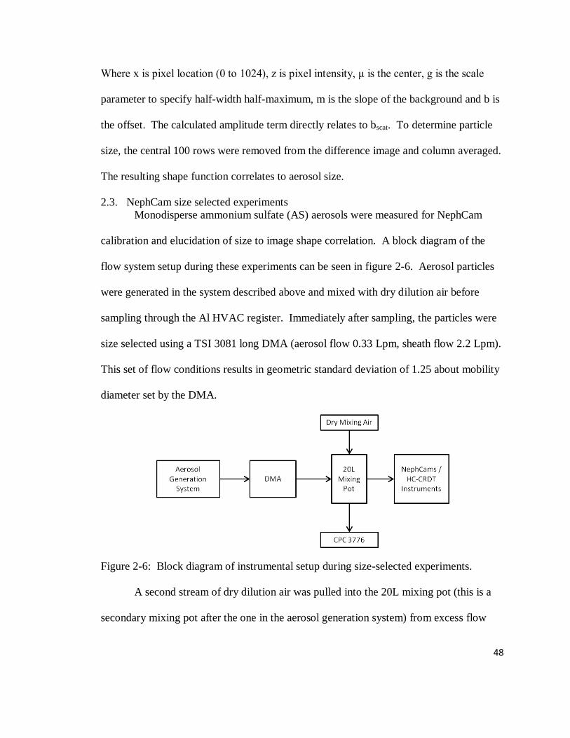
48
Where x is pixel location (0 to 1024), z is pixel intensity, μ is the center, g is the scale
parameter to specify half-width half-maximum, m is the slope of the background and b is
the offset. The calculated amplitude term directly relates to bscat. To determine particle
size, the central 100 rows were removed from the difference image and column averaged.
The resulting shape function correlates to aerosol size.
2.3. NephCam size selected experiments
Monodisperse ammonium sulfate (AS) aerosols were measured for NephCam
calibration and elucidation of size to image shape correlation. A block diagram of the
flow system setup during these experiments can be seen in figure 2-6. Aerosol particles
were generated in the system described above and mixed with dry dilution air before
sampling through the Al HVAC register. Immediately after sampling, the particles were
size selected using a TSI 3081 long DMA (aerosol flow 0.33 Lpm, sheath flow 2.2 Lpm).
This set of flow conditions results in geometric standard deviation of 1.25 about mobility
diameter set by the DMA.
Figure 2-6: Block diagram of instrumental setup during size-selected experiments.
A second stream of dry dilution air was pulled into the 20L mixing pot (this is a
secondary mixing pot after the one in the aerosol generation system) from excess flow

49
caused by the HC-CRDT pumps and the CPC. While this secondary dilution was not
desirable because it greatly reduced monodisperse particle concentration it was necessary
to minimize ambient air leakage into the HC-CRDT from pressures significantly below
ambient.
AS was used as the test aerosol because absorption is negligible - ring-down and
NephCam measurements equivalent - has a moderate ERH between 37 and 40% (Tang
and Munkelwitz 1994) and crystallizes to a near spherical shape so Mie theory can be
applied. Prior to size selection, it was necessary to dry the aerosol to below the ERH.
This ensured that the particle sizes selected by the DMA were equivalent to the particle
sizes reaching the NephCams and HC-CRDT; had particles been non-effloresced prior to
sizing, particle diameter can change due to fluctuations in RH. The humidifier and dryer
were removed from the HC-CRDT for these experiments for similar reasons.
2.3.1. "Drift-down" experiments
The size-selected experiments were done as "drift down" experiments; particle
concentration (and extinction/scattering) was started high and allowed to slowly decrease
in time; the impactor on the DMA became clogged with salt from the high concentrations
of AS solution required (1500 - 16000 ppm). Depending upon salt solution
concentration, experiments would last between 2 and 8 hours; higher salt solution
concentrations had shorter experiment lengths. In very high salt limit, multiple data sets
were run. Data collection was stopped when there was not enough aerosol reaching the
HC-CRDT for detection.
2.4. HC-CRDT
2.4.1. Theory of operation

50
The use of cavity ring-down has been well documented, so only a brief review
will be presented here (Bulatov, Fisher et al. 2002; Atkinson 2003; Moosmuller, Varma
et al. 2005). A conceptual diagram of a cavity ring-down transmissometer (CRDT) can
be seen in Figure 2-7 below:
Figure 2-7: Conceptual diagram of a cavity ring-down instrument.
Nanosecond laser pulses are injected into an optical cavity formed from two
highly reflective (R > 99%) mirrors. The intra-cavity intensity decays exponentially due
to absorption, scattering and mirror transmission as the beam traverses the cavity
(eq 2-3 )
where I0 and I are the initial beam intensity and the intensity at time t, and β is the decay
constant (s-1
). Decay constants in units of inverse length Mm-1
are obtained using the
speed of light
(eq 2-4)
Our preferred unit of measurement is the inverse megameter (Mm-1
) which corresponds
to a loss of 1 part per million of the light per meter of air traversed. In practice, the intra-
mirror cavity length and the length of the aerosol sample inside the cavity are not
equivalent. To account for this difference, a correction of the ratio of lengths is applied

51
(eq 2-5)
where lcavity and laerosol are the cavity and aerosol length. Extinction coefficients (bext) for
aerosols can be determined by calculating the difference in decay constants between the
aerosol sample and a clean air background. Mathematically:
(eq 2-6)
Clean air is generated by passing the aerosol sample through a HEPA filter to remove all
radiatively significant particles.
2.4.2. Physical construction
A Humidity Controlled – Cavity Ring-Down Transmissometer (HC-CRDT) was
developed in our lab. A detailed block diagram of the HC-CRDT can be seen in figure 2-
8. A system of 4 aerosol flow lines and ring-down cavities each incorporating 3 laser
wavelengths (λ = 355, 532, 1064 nm) was constructed for the measurement of extinction
by aerosol particles as a function of relative humidity. These 4 independent aerosol
flow/CRD systems will be referred to as channels. Depending upon the type of
experiment being conducted – intra-cavity comparison, humidity control investigation, or
ambient measurements/field work – the HC-CRDT can be operated in different flow
modes. Since only laboratory experiments were performed, the 4 channels will be
referred to as Ambient-A, Ambient-B, Dry and Humidified. In the field, a slightly
different flow setup is used.
Nanosecond laser pulses are generated by an Nd:YAG laser (Big Sky Laser
CFR200, 15 Hz) at the fundamental and 2nd
and 3rd
harmonics; 1064 nm, 532 nm and
355 nm, respectively. These laser pulses are transferred to the instrument via fiber optic
bundles. A separate fiber optic bundle is used for each wavelength. A single fiber optic

52
Figure 2-8: Schematic of the HC-CRDT instrument.

53
bundle is split in quadrature to deliver each given wavelength to all 4 channels
simultaneously.
Prior to cavity delivery, laser pulses are shaped by 2 lenses; a 3 mm diameter x 3
mm focal length plano-convex mounted to the end of the fiber bundle and a 10 mm
diameter x 500 mm focal length plano-convex in a focusing block ~1" from the cavity
mirror. This results in a scrambling of the "spotty" image produced by the individual
fibers in the bundle and a rough (~ 0.5 cm diameter) focusing of the laser intensity at the
opposite mirror. The 355 nm and 532 nm laser pulses also pass through a corresponding
bandpass filter to remove residual contributions of other wavelengths (1064 and 532 nm
in the 355 nm, and 1064 nm and 355 nm in the 532 nm).
Each wavelength is contained within the optical cavity by a pair of highly
reflective mirrors: 1064 nm (Layertec, LLC., r = 1000 mm, R > 99.98%), 532 nm
(Layertec, r = 1000 mm, R > 99.98%), and 355 nm (Layertec, r = 1000 mm, R > 99.9%).
The 3 mirrors are positioned in a triangular pattern so that the optical path of each
wavelength is parallel to the cavity axis and aerosol flow.
Light exiting the cavity for each wavelength is passed through a corresponding
Schott glass cutoff filter and a 10 mm diameter 100 mm focal length plano-convex lens
before reaching a detector. Detector signals are carried by 3 m long SMB co-axial cables
to a pair of National Instruments PXI-5150 high speed 8 channel digitizers mounted in a
National Instruments PXI-8105 (2.0 GHx Intel Core Duo T2500 dual core-processer, 512
MB dual channel 667 MHX DDR2 RAM, Windows XP) chassis. This design allows for
the rapid and real-time collection of the decay signals because the fast A/D conversion is
directly present on the PCI bus, allowing signals to be collected and processed at high
54
speed and overall high throughput. All 12 data streams – 4 channels with 3 wavelengths
each – can be digitized, processed and stored simultaneously at the operating speed of the
laser (15 Hz). Data collection and processing is controlled by custom LabView 2010
vi’s.
Data collection is initiated by triggering data acquisitions off the laser’s Q-switch
synch line. Analog voltages from all 12 detectors are sampled for approximately 68 µsec
corresponding to a data string of 4096 points. From the full 4096 data points, a portion is
dropped on the front end to remove the non-exponential portion of the signal. Exact
magnitude of truncation varies slightly by channel depending upon total light intensity
transmitted by the individual fibers, but is in the range of 200, 400 and 0 points for the
IR, Vis and UV, respectively. The exponential decay constant of each ring-down signal
is then calculated using the direct sums algorithm (Everest and Atkinson 2008). Data
array lengths are further truncated to a number of samples that corresponds to 6 times the
1/e time from the previous decay (5 – 7 η was determined to be the best compromise for
relevant noise levels) (Everest and Atkinson 2008). After calculation of the exponential
decay constants, this data is logged to an Excel comma separated values (CSV) file and
the raw ring-down data is discarded. Thus 12 ring-down decay constants are recorded
from a single laser pulse 15 times per second (180 Hz real-time measurement rate).
Separate but identical optical cavities exist for each of the 4 channels. Aerosols
enter and exit a 1 m long 34 mm square extruded aluminum tube (ThorLabs XT34
system, 29 mm ID) at either end through 3/4" tube ports at 45° angles to minimize flow
disturbances (figure 2-8). To prevent mirror contamination, a filtered air back-flush flow
is generated. A double-headed peristaltic pump (Stenner Pump Company 170DM5)
55
circulates air through a HEPA filter and the dead space between the mirrors and aerosol
flow ports on all 4 channels. Since only a single double-headed peristaltic pump is used,
a single head must be used as the backflush for both ends of a pair of channels. This
translates to the backflush air flow being split end-to-end and then between a pair of
cavities. Flow lines are recombined for return to the peristaltic pump. Total backflush
flow to one end of a single channel is 50 cc/min. To minimize "cross-talk" between the
backflush streams, air enters between two cavities and exits on the periphery.
The main aerosol flow through the HC-CRDT is controlled by a pair of linear
pumps (EMS MegaLite IAQ Pump, Model # 6025SE-V) at 2.0 Lpm; 1.0 Lpm flow per
channel. Since a single head of the peristaltic pump is split between a pair of channels, it
was also necessary to pull aerosol flow using a single pump split between the same pairs
of channels. This prevents "cross-talk" between the channels from the common
backflush connection and small variations in aerosol flow. The Ambient-A and Dry
channels form one flow pair while the Ambient-B and Humidified channels form another
flow pair.
All aerosol containing parts were constructed from metal (Cu or Al) to minimize
static charging or water adsorption effects and consequent loss of particles. All metal
pieces were grounded at various locations throughout the system using wire to eliminate
local static charging.
The determination of aerosol extinction coefficients requires that the extinction of
both particle-laden and particle-free air be measured separately, as mentioned in the
discussion of eq. 2-6. Particle-laden air is directly sampled; while particle-free air is
obtained by passing the same aerosol through a HEPA filter (Whatman Hepa-Cap) using

56
a pair of electrically actuated 3-way valves (Assured Automation 31DXV4). Separate
valves and HEPA filters were installed for each channel (see figure 2-8) and are computer
controlled by a Measurement Computing relay board (USB-ERB08, 8-channel
electromechanical) and custom LabView 2010 vi's.
2.4.3. RH sensors and location
Relative humidity and temperature are also measured every second at various
points in the instrument (figure 2-8) using six Vaisala HMP50 RH/T sensors. (A seventh
RH/T sensor is present on the Dry Valve, however the temperature measurement has
malfunctioned.) These sensors are connected in line with the flow system using Ultra-
Torr vacuum fittings. Digitization and archival of the 1 Hz relative humidity and
temperature measurements is accomplished using a high speed 8 channel 16 bit A/D
converter (Measurement Computing USB-1616FS) controlled by custom LabView 2010
vi’s.
2.4.4. Humidifier/Dryer
The relative humidity of the Humidified and Dry channels is controlled using a
humidifier and dryer, respectively, fashioned after the commercially available TSI 3062
Diffusion Dryer. Aerosols traverse the humidifier and dryer through a 2 foot section of
1" diameter stainless steel perforated tube (La Choppers, 1/8" diameter holes, 3/8"
staggered centers) surrounded by a stainless steel mesh. Dryer and humidifier are
connected to HC-CRDT flow lines using 1/2" Swagelok fittings. The external casing of
the dryer was made from a 3" OD, 2 3/4" ID acrylic tube with properly sized end caps.
The void between the stainless tube and acrylic tube was filled with Silica gel desiccant
(Fisher Scientific, indicating, 4-8 mesh). The acrylic tube diameter of the dryer is larger
than that of the humidifier to allow for easier desiccant exchange through 1/4" NPT
57
plugs. The external casing of the humidifier was made from a 1 3/4" OD, 1 1/4" ID
acrylic tube with properly sized end caps. The stainless steel tube in the humidifier was
wrapped using water wick (Wickstore.com #756). An external water reservoir supplies a
constant water flow through the wick to the humidifier. Excess water from the wick
drains to a reservoir to avoid entrapment in flow lines. Stainless steel mesh surrounding
stainless perforated tube was included to prevent desiccant and water wick from entering
the aerosol particle flow line and scavenging aerosol. End to end electrical conductivity
(< 10 Ω) of the humidifier and dryer (across Swagelok fittings and stainless steel tube)
was checked periodically for the prevention of particle loss to static charging.
2.4.5. Data processing and analysis
The HC-CRDT measures the total extinction coefficients of a bulk aerosol sample
(bext,TOT). This total extinction includes losses from aerosol (bext,aerosol), background air
(bext,bkg), mirror transmission (bext,mirrors) and any other non-aerosol extinction loss (bother):
(eq 2-7)
The measurement of aerosol extinction coefficients requires the separation of extinction
due to the presence of aerosol (bext,aerosol) and all other losses. Experimentally, this is
accomplished by passing the aerosol flow through a HEPA filter to remove the aerosol
particles. These "clean air" cycles allow for the measurement of a single extinction
coefficient that represents the extinction caused by all non-aerosol loss mechanisms
(background, mirrors, other). The clean air background signal changes slowly in time, so
a linear regression of background extinction versus time is performed on the clean cycles
on either side of an aerosol cycle. These background subtractions are performed using
LabView 2010 vi’s on all ring-down data.

58
2.5. Allan Variance
An Allan Variance analysis was performed on the HC-CRDT to determine
instrument stability as a function of random noise and drift. It also serves as a measure
for the minimum variance in a measurement as a function of integration time. To
perform the Allan Variance, dry, filtered air was sampled by the HC-CRDT for 24 hours.
Valve control on the HC-CRDT was disabled and all valves were left in the clean state.
Data analysis was done using an Igor Pro (Wave Metrics, v. 1.6.2.1) script obtained from
Andrew Freedman at Aerodyne, Inc (Freedman 2009).
2.6. Humidification experiments
2.6.1. Flow system setup
For the humidification experiments, a slightly different flow setup was used to
allow for the measuring of extinction coefficients of a polydisperse aerosol. A block
diagram of the flow system can be seen in figure 2-9.
Figure 2-9: Block diagram of flow system setup for Humidification experiments.
Aerosols produced in the aerosol generation system were mixed with dilution air.
of varying humidities ranging between approximately 50% and 10% RH. RH of the
dilution air was controlled by a split line on the dilution air stream that allowed the air
stream to pass through a dryer and/or bubbler to lower or raise the humidity, respectively.
59
The RH of the system was allowed to stabilize at either dry (~ 10%) or wet (~ 50%) prior
to starting data collection. After a couple of data cycles, the dilution air flow was
changed slightly to raise or lower the ambient RH, respectively. In the experiments
where RH was increased from dry to wet, some of the data in the transition region had to
be removed due to the presence of water droplets getting into the flow lines. During the
RH decreasing experiments, this was not a problem since the system was allowed to
equilibrate and remove all water droplets before data collection began.
Aerosols were directly sampled into the secondary 20L mixing pot through a
URG-2000-30EQ cyclone. Total flow of all instruments was approximately 6.0 Lpm
corresponding to a cut-point of 1.0 μm at the cyclone. A secondary dilution was not
implemented to maintain a consistent RH within the second mixing pot. Also, sufficient
flow from aerosol generation was available so sampling through the cyclone did not
induce ambient air leakage into the HC-CRDT (sampling very near ambient pressure).
The DMA was operated in scanning mode with a TSI CPC3776 downstream for
the measurement of size distributions. Sheath and aerosol flows were set to 1.15 and 2.2
Lpm, respectively. Scan time was 180 sec up with a 15 sec retrace. The ratio of sheath
to aerosol flows results in a tradeoff between the sharpness of cutoff for a given size bin
and total width of the size distribution. We chose to maximize the width of the collected
size distributions (16.8 nm to 982.2 nm) to most closely mimic the particle sizes passing
through the cyclone. A TSI CPC 3007 was operated in parallel to measure total particle
concentration in addition to the size distribution measurement.
Correction factors for particle transmission through the HC-CRDT were
calculated for this flow system using AS aerosols. Humidity controls were not used for
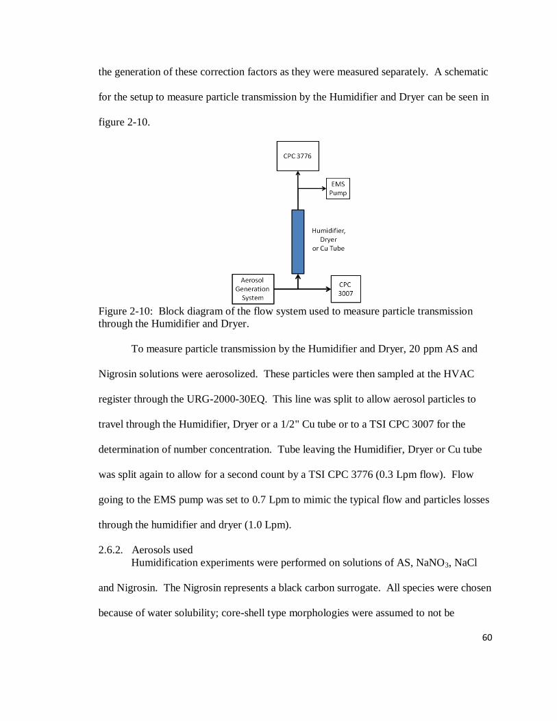
60
the generation of these correction factors as they were measured separately. A schematic
for the setup to measure particle transmission by the Humidifier and Dryer can be seen in
figure 2-10.
Figure 2-10: Block diagram of the flow system used to measure particle transmission
through the Humidifier and Dryer.
To measure particle transmission by the Humidifier and Dryer, 20 ppm AS and
Nigrosin solutions were aerosolized. These particles were then sampled at the HVAC
register through the URG-2000-30EQ. This line was split to allow aerosol particles to
travel through the Humidifier, Dryer or a 1/2" Cu tube or to a TSI CPC 3007 for the
determination of number concentration. Tube leaving the Humidifier, Dryer or Cu tube
was split again to allow for a second count by a TSI CPC 3776 (0.3 Lpm flow). Flow
going to the EMS pump was set to 0.7 Lpm to mimic the typical flow and particles losses
through the humidifier and dryer (1.0 Lpm).
2.6.2. Aerosols used
Humidification experiments were performed on solutions of AS, NaNO3, NaCl
and Nigrosin. The Nigrosin represents a black carbon surrogate. All species were chosen
because of water solubility; core-shell type morphologies were assumed to not be

61
occurring for modeling of the water uptake and change in optical properties by these
aerosols.

62
3. Results & Discussion - NephCam experiments
3.1. NephCam characterization and getting good image results
The NephCams were constructed using a CCD so both shape and intensity
information could be obtained for scattering measurements. As with any camera or
imaging system, characterization of the physical design (optics and image collection
surface at the CCD) is necessary to produce images of optimal quality so the most
information can be extracted from an image.
The quality of an image generated in any photographic system is ultimately a
function of the lens system employed. The aberrations, or imperfections, in an image can
be classified into 6 primary types: spherical aberration, coma, astigmatism and field
curvature, oblique spherical aberration, distortion and chromatic effects (Cox 1966). For
the NephCam setup employed, oblique spherical aberration and chromatic effects do not
need to be considered; these are only present when multiple wavelengths are used. The
diode laser employed in the NephCams operates at 532 nm. Each aberration has its own
effect on image quality and the resulting image; however, the complete removal of all
aberrations is impossible due to the opposing nature of many aberrations.
3.1.1. Targets
Lens curvature results in spherical aberrations; not all rays passing through a
spherical surface are imaged to the same point. It arises from light entering at the edge of
the optic being focused to slightly different location than light entering near the center of
the optic as shown in figure 3-1. The presence of spherical aberrations can result in
radial blur and astigmatism; images appear to blur towards the edges and different lines
of focus in an image are obtained. This effect worsens as the aperture is stopped down
(closing of the aperture, higher f-stop) and is directly linked to light diffraction by the
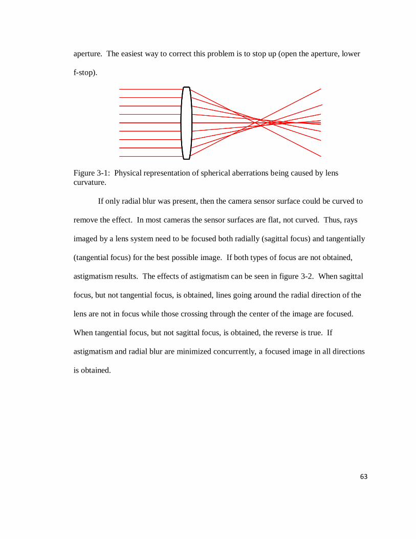
63
aperture. The easiest way to correct this problem is to stop up (open the aperture, lower
f-stop).
Figure 3-1: Physical representation of spherical aberrations being caused by lens
curvature.
If only radial blur was present, then the camera sensor surface could be curved to
remove the effect. In most cameras the sensor surfaces are flat, not curved. Thus, rays
imaged by a lens system need to be focused both radially (sagittal focus) and tangentially
(tangential focus) for the best possible image. If both types of focus are not obtained,
astigmatism results. The effects of astigmatism can be seen in figure 3-2. When sagittal
focus, but not tangential focus, is obtained, lines going around the radial direction of the
lens are not in focus while those crossing through the center of the image are focused.
When tangential focus, but not sagittal focus, is obtained, the reverse is true. If
astigmatism and radial blur are minimized concurrently, a focused image in all directions
is obtained.

64
Figure 3-2: Physical representation of astigmatism in the sagittal (middle) and tangential
(right) focus. The left image represents an image where astigmatism is not present.
Figure 3-3: Image of target by digital Nikon D40, 9 MPixel SLR camera backlit with
ambient lighting. Target has been white balanced and corrected to give maximum
contrast and highlight shape.
Figure 3-4: Normalized NephCam images of the target in the figure 3-3 with aperture
settings of 1.6 (left), 4 (center) and 8 (right).
Maximum image intensity for all targets is slightly off center. This resulted from
the 1" light-harvesting lens not being perfectly centered over the CCTV lens. This effect
was corrected during actual NephCam operation, but the effects of astigmatism are still
evident. The 1.6 aperture setting does a very good job of reproducing the original target
image. As the aperture is stopped down, signs of sagittal blur are evident and worsen
1.0
0.9
0.8
0.7
0.6
0.5
1.0
0.8
0.6
0.4
0.2
1.0
0.8
0.6
0.4
0.2
1.0
0.8
0.6
0.4
0.2
0.0

65
with decreasing aperture size (higher f number). The tangential focus in all of the images
is good; vertical and horizontal crossing lines are recreated well at all aperture settings.
3.1.2. Calibration matrix
Distortions are classified as either pincushion or barrel types; straight lines on an
image appear to bow inward or outward, respectively, like the shape of a pincushion or
barrel. Figure 3-5, shows the general shape of barrel versus pincushion distortions; left
and right, respectively.
Figure 3-5: Square grid without distortion (left), barrel distortion (center) and pincushion
distortion (right).
Coma can arise from distortions. When imaged rays do not originate on the
optical axis, but somewhere off axis, images exhibit a "comet" like shape with intensity
diffusing away or towards the center of the image as shown in figure 3-6.
Figure 3-6: Physical representation of image coma; dots not located at image center
show comet-like tails extending away from center.
Calibration dot matrices are useful for determining the presence of coma,
pincushion and barrel distortions. Points are arranged along a grid in both the horizontal
and vertical directions with regular spacing. If either pincushion or barrel distortions are
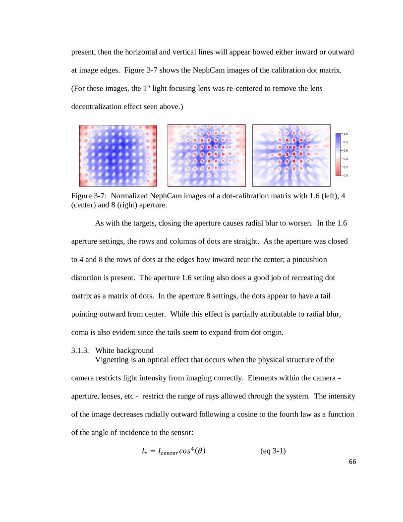
66
present, then the horizontal and vertical lines will appear bowed either inward or outward
at image edges. Figure 3-7 shows the NephCam images of the calibration dot matrix.
(For these images, the 1" light focusing lens was re-centered to remove the lens
decentralization effect seen above.)
Figure 3-7: Normalized NephCam images of a dot-calibration matrix with 1.6 (left), 4
(center) and 8 (right) aperture.
As with the targets, closing the aperture causes radial blur to worsen. In the 1.6
aperture settings, the rows and columns of dots are straight. As the aperture was closed
to 4 and 8 the rows of dots at the edges bow inward near the center; a pincushion
distortion is present. The aperture 1.6 setting also does a good job of recreating dot
matrix as a matrix of dots. In the aperture 8 settings, the dots appear to have a tail
pointing outward from center. While this effect is partially attributable to radial blur,
coma is also evident since the tails seem to expand from dot origin.
3.1.3. White background
Vignetting is an optical effect that occurs when the physical structure of the
camera restricts light intensity from imaging correctly. Elements within the camera -
aperture, lenses, etc - restrict the range of rays allowed through the system. The intensity
of the image decreases radially outward following a cosine to the fourth law as a function
of the angle of incidence to the sensor:
(eq 3-1)
1.0
0.9
0.8
0.7
0.6
1.0
0.9
0.8
0.7
0.6
0.5
0.4
0.3
1.0
0.8
0.6
0.4
0.2
1.0
0.8
0.6
0.4
0.2
0.0

67
Where Ir is the light intensity at some radial distance r from the center, Icenter is the
intensity at the center and θ is the axial angle between Ir and Icenter. Figure 3-8 shows this
radial decrease mapped to an image.
Figure 3-8: Cause (left) and effect (right) of vignetting in an image.
This radial decrease in light can be larger than predicted by the cosine relationship
due to the physical construction of the camera; the cos4 relationship represents the best
case scenario. Vignetting can be avoided by stopping down the aperture and thus works
in opposition to spherical aberrations.
A sheet of white paper served as a background for image collection. The
resulting images by the NephCams at aperture settings of 1.6 (left), 4 (middle) and 8
(right) can be seen in figure 3-9. These images have not been normalized to show
intensity effects. The image of a white background will show the presence or absence of
vignetting; images should have a flat intensity. If vignetting is present, then the
background image will appear curved.
100
95
90
85
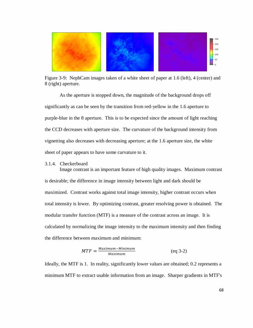
68
Figure 3-9: NephCam images taken of a white sheet of paper at 1.6 (left), 4 (center) and
8 (right) aperture.
As the aperture is stopped down, the magnitude of the background drops off
significantly as can be seen by the transition from red-yellow in the 1.6 aperture to
purple-blue in the 8 aperture. This is to be expected since the amount of light reaching
the CCD decreases with aperture size. The curvature of the background intensity from
vignetting also decreases with decreasing aperture; at the 1.6 aperture size, the white
sheet of paper appears to have some curvature to it.
3.1.4. Checkerboard
Image contrast is an important feature of high quality images. Maximum contrast
is desirable; the difference in image intensity between light and dark should be
maximized. Contrast works against total image intensity, higher contrast occurs when
total intensity is lower. By optimizing contrast, greater resolving power is obtained. The
modular transfer function (MTF) is a measure of the contrast across an image. It is
calculated by normalizing the image intensity to the maximum intensity and then finding
the difference between maximum and minimum:
(eq 3-2)
Ideally, the MTF is 1. In reality, significantly lower values are obtained; 0.2 represents a
minimum MTF to extract usable information from an image. Sharper gradients in MTF's
250
200
150
100
50
0
250
200
150
100
50
0
250
200
150
100
50
0
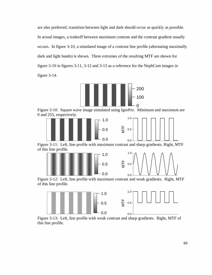
69
are also preferred; transition between light and dark should occur as quickly as possible.
In actual images, a tradeoff between maximum contrast and the contrast gradient usually
occurs. In figure 3-10, a simulated image of a contrast line profile (alternating maximally
dark and light bands) is shown. Three extremes of the resulting MTF are shown for
figure 3-10 in figures 3-11, 3-12 and 3-13 as a reference for the NephCam images in
figure 3-14.
Figure 3-10: Square wave image simulated using IgorPro. Minimum and maximum are
0 and 255, respectively.
Figure 3-11: Left, line profile with maximum contrast and sharp gradients. Right, MTF
of this line profile.
Figure 3-12: Left, line profile with maximum contrast and weak gradients. Right, MTF
of this line profile.
Figure 3-13: Left, line profile with weak contrast and sharp gradients. Right, MTF of
this line profile.
200
100
0
200
100
0
1.0
0.5
0.0
1.0
0.5
0.0
1.0
0.5
0.0
MT
F
1.0
0.5
0.0
1.0
0.5
0.0
1.0
0.5
0.0
MT
F
1.0
0.5
0.0
1.0
0.5
0.0
1.0
0.5
0.0
MT
F

70
In figure 3-11, ideal contrast is obtained. A distinct sharp edge between light and
dark is visible. This is evident in the image shape (left) and MTF (right) by the sharp
transition from light to dark (1 to 0). In figures 3-12 and 3-13, ideal contrast is not
obtained. In figure 3-12, the transition from light to dark is smooth with a range of
intermediate gray values. The plot of MTF (right) mirrors this non-ideality. In figure 3-
13, the contrast gradient is very sharp, however total contrast between light and dark is
decreased (0.5 to 1 instead of 0 to 1). Actual camera systems typically operate
somewhere between the extremes in figures 3-12 and 3-13. Ideal contrast, figure 3-11, is
rarely achieved.
Images of checkerboards provide a good diagnostic tool for image contrast and
modular transfer functions. An image of the actual checkerboard used is shown in figure
3-14. The checkerboard images taken using the NephCams are shown in figure 3-15 for
aperture settings of 1.6 (left), 4 (middle) and 8 (right).
In an ideal MTF, the transition between light and dark should be quick and hold
the maximum or minimum values across the light or dark spot, respectively. If our
checkerboard was perfect then these transitions would be seen as sharp transitions
between the light and dark. However, these checkerboards were produced using a Xerox
photocopier; the checkerboard pattern is not perfect and the transitions between light and
dark are not as sharp as seen in figure 3-14 (that figure has been white balanced and
contrast corrected for clarity). So, steeper gradient between light and dark represent a
better MTF.
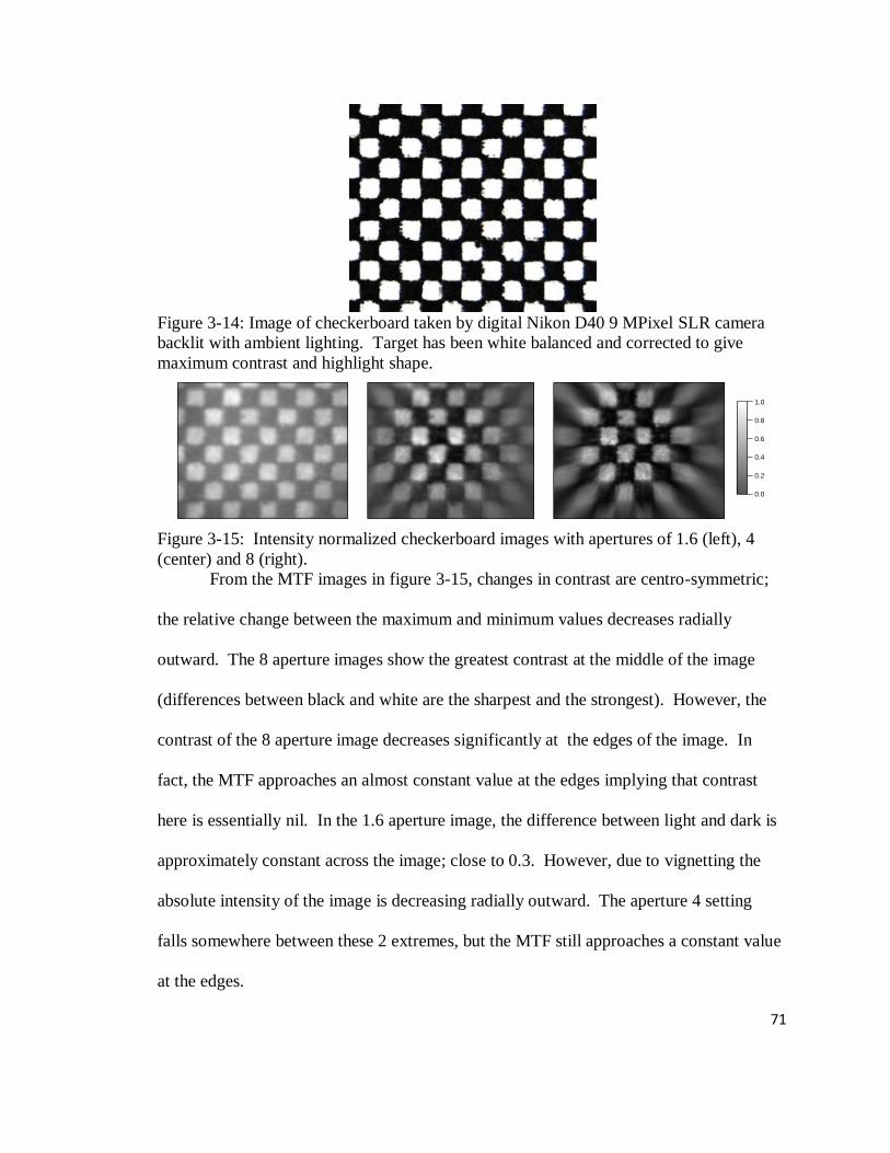
71
Figure 3-14: Image of checkerboard taken by digital Nikon D40 9 MPixel SLR camera
backlit with ambient lighting. Target has been white balanced and corrected to give
maximum contrast and highlight shape.
Figure 3-15: Intensity normalized checkerboard images with apertures of 1.6 (left), 4
(center) and 8 (right).
From the MTF images in figure 3-15, changes in contrast are centro-symmetric;
the relative change between the maximum and minimum values decreases radially
outward. The 8 aperture images show the greatest contrast at the middle of the image
(differences between black and white are the sharpest and the strongest). However, the
contrast of the 8 aperture image decreases significantly at the edges of the image. In
fact, the MTF approaches an almost constant value at the edges implying that contrast
here is essentially nil. In the 1.6 aperture image, the difference between light and dark is
approximately constant across the image; close to 0.3. However, due to vignetting the
absolute intensity of the image is decreasing radially outward. The aperture 4 setting
falls somewhere between these 2 extremes, but the MTF still approaches a constant value
at the edges.
1.0
0.8
0.6
0.4
0.2
0.0
1.0
0.8
0.6
0.4
0.2
0.0
1.0
0.8
0.6
0.4
0.2
0.0

72
These MTF's point to design constraints in NephCam image quality. The
NephCams require the ability to tell light from dark - i.e. what is being measured as
scattering and what is not? The smaller apertures allows for greater sensitivity to
scattering in the middle of the image but little at the edges. The larger aperture does not
give optimal sensitivity, actually it is just above the usable limit, but the sensitivity across
the image is nearly constant. The implication is that if vignetting can be corrected at the
larger aperture settings, then the 1.6 aperture can produce the best images. With the
smaller aperture settings, the sensitivity may be greater but ultimately the angular
scattering information near the edges of the images is lost, which is undesirable. It is
harder to account for imperfections in the MTF if the MTF is not constant across the
image, but imperfections in the absolute MTF (contrast) can be corrected if the MTF is
constant.
3.1.5. Single line
To mimic the distribution of laser light measured by the NephCams, pieces of
black masking tape were used on a white sheet of paper to create a single white line on an
otherwise black background. The line was approximately 3 mm thick and was imaged
using the same LED box setup as before. The collected images of the single line are
shown in figure 3-16.
Figure 3-16: Normalized NephCam images of a single line with aperture settings of 1.6
(left), 4 (center) and 8 (right).
1.0
0.8
0.6
0.4
0.2
1.0
0.8
0.6
0.4
0.2
0.0
1.0
0.8
0.6
0.4
0.2
0.0
1.0
0.5
0.0

73
The white line shows the culmination of all of the imaging effects observed
above. As the aperture is stopped down, image intensity is blurred more in the radial
direction. The single line appears to have wings along the x-axis of the image at smaller
apertures. The decrease in contrast near the edges of the image are also evident at
smaller apertures; there is a loss in distinction between the white line and the background.
Vignetting is also evident in the 1.6 aperture image; near the center of the image the
background intensity is significantly higher than at the edges. However at this aperture
setting the imaged line and background are clearly distinct across the entire image. As a
result, the 1.6 aperture was chosen as the operational setting for the NephCam.
3.2. NephCam size based calibration experiments
The NephCam was initially calibrated using size-selected aerosols; polydisperse
aerosols contain too much information and variation to initially characterize the
NephCam response. By limiting the aerosols present to a narrow size bin, the effects of
size on both collection efficiency (and thus calibration slope) and image shape could be
elucidated. An optical response model of light scattering collected by the NephCam was
constructed as a theoretical comparison to the measured data.
Using the physical parameters of the NephCams, ray tracing methods were
employed to determine what the image shape collected by the NephCams should look
like as a function of particle size. The intermediate goal was to be able to apply the
NephCam response model to a distribution of aerosol particles to see if the measured and
modeled image shapes correlated. The end goal is to be able to invert observed image
shapes for size distribution information, however that goal is beyond the scope of this
work.

74
The design of the NephCams and the basic parameters used in the model are
illustrated in figure 3-17. The x- and y-axes are in the horizontal and vertical directions,
respectively. All components of camera and aerosols are assumed to be centered and
positioned relative to (0,0). A collection of aerosol particles (black, red and purple dots)
are assumed to be in line with the laser beam (green line, hν) which propagates from left
to right (backward to forward scattering, respectively); these aerosols have location
(x0,y0) relative to (0,0). A 1" plano-convex light-harvesting lens is placed at its focal
length (Df) above (0,0). A CCTV lens for image collimation and magnification is placed
above the back edge of the focusing lens at distance DCCTV. The CCD is above the output
face of the CCTV lens by distance DCCD.
The naming convention used presently is: Point locations in the model are
defined by lowercase (xn,yn) values. The uppercase values represent physical distances in
the real setup like the focal length (Df) and offset distance between the light-harvesting
lens and CCTV (DCCTV). The vector propagating away from a point (xn, yn) is (dxn, dyn).
The angle of incidence of the vector (xn, yn) + (dxn, dyn) to a surface are Greek
letters with the subscript n (i.e. αn). The angle of departure of the vector (xn, yn) + (dxn,
dyn) are Greek letters with the subscript n+1 (i.e. αn+1). Greek letters are incremented as
different parts of the camera system are traversed; α, β, ε correspond to the front edge of
the light harvesting lens, the back edge of the light harvesting edge and the CCTV lens,
respectively. The letters γ and δ were omitted to avoid confusion with y and d.
The model was built in x, y space only, whereas the actual NephCams operate in
real space; x, y, z. All of the model calculations are a simulation of centerline image
along the horizontal image when particles are at the maximum laser beam intensity. The

75
Figure 3-17: Physical design of NephCam and relevant parameters for defining the
optical response model. Three discrete aerosol particles and the laser beam are
represented by black, red and purple dots and a green line at the bottom of the figure. The
CCD detector is the green bar at top and the main light-harvesting lens is shown in dark
blue. The CCTV lens system is shown in gray and the lenses on either side as blue bars.
Scattered radiation propagating through the camera is shown as black arrows. Normal
vectors are shown as orange double-headed arrows.

76
diode laser used presently has a radially symmetric Gaussian intensity. Thus, the images
generated by this model correspond to particles that pass directly through the center of
the laser beam. On either side of the laser beam (horizontally) the intensity of the laser
drops off as defined by the Gaussian profile. The mapping of a 3-D Gaussian surface to a
2-D image results in a Lorentzian image shape. The radial symmetry of the laser beam
along the z-axis allows for the conservation of phase function and size information along
this axis with intensity being the only changing parameter.
To trace rays through the system, the location of aerosol particles must first be
defined. In x, y space:
(eq 3-3)
where xaerosol, yaerosol is the location of the aerosol particles. In keeping with the naming
conventions used throughout the rest of the model, the location (xaerosol, yaerosol) will be
referred to as (x0,y0). For simplicity, all real positions and distances (in the model's x, y
space) will be given in the units of pixels for ease of mapping points to the ThorLabs
DCU224M's CCD (1280 pixels along x, 1 pixel equals 4.65μm) instead more familiar
units of inches or mm.
The relative intensity and direction of light scattered by a particle is governed by
the phase function, which is a function of both the refractive index and size parameter (χ).
In x, y model space, the direction and intensity of scattered photons can be represented
by:
(eq 3-4)
77
where θ is the angle between forward laser propagation and the scattered radiation and P
is the power of the scatter. The points along the light-harvesting lens that are able to
collect scattered light are constrained such that angle between the incident radiation (α1)
and lens normal ( ) are less than 90°; it is physically impossible to collect
scattered light at obtuse angles using this design. The scattering angles (θ) that actually
reach the CCD range between 65° and 115° depending upon the aerosol particle's x
location within the laser beam.
The focal length and thus the location of the front edge of the light-harvesting lens
can be calculated by first applying the lens maker’s equation to the 1" focusing lens:
(eq 3-5)
Where Df is the focal length, n is the refractive index of the lens, and R1 and R2 are the
radii of curvature of the front and back sides of the lens, respectively. The light-
harvesting lens in the NephCams is a plano-convex lens; therefore R2 = ∞. Locations on
the front side of the lens (x1, y1) can then be calculated from:
(eq 3-6)
Where x is the x location of the points along the lens, R1 is radius of curvature of the
front side of the lens as calculated from eq 3-5, and Df is the focal length. The location of
the 1" lens is assumed to be located Df pixels above (0,0). The scattering angle (θ)
intersecting a point on the lens (x1,y1) is calculated from:
(eq 3-7)

78
where (x1,y1) is dictated by equation 3-6 and (x0,y0) is the location of the aerosol particle
and I is a scalar to make the points intersect. The normal vector to the light harvesting
lens ( ):
(eq 3-8)
The angle between the scattered radiation and lens normal (α0) is calculated using the dot
product:
(eq 3-9)
The cos(α0) also serves as a weighting term for the collection efficiency of the 1" lens
relative to the angle of incidence. For computational efficiency, the model is iterated
across all lens points that could collect scattered radiation, rather than across the entire
range of scattering angles θ (0° - 180°). This implies that radiation can only be collected
by pixels between the tangential crossing of the lens in either the maximum or minimum
direction. This tangential crossing occurs when the lens normal and scattered radiation
are orthogonal (α1 = 90°). Using this approach, the angle of scattered radiation is
determined from the location of the aerosol particle and the current lens location being
used. (Computationally and programmatically this method is easier than trying to trace
each ray as a function of θ through the lens.)
Using Snell’s law, the scattered radiation is refracted towards the lens normal (α1)
upon entering the lens:
(eq 3-10)

79
where n0 and n1 are the refractive indices of air (1) and quartz (1.519473), respectively.
The vector that propagates through the light-harvesting lens (dx,1, dy,1) is calculated from
the normal vector to the back side of the front of the light-harvesting lens ( ):
(eq 3-11)
The vector (dx1, dy1) is calculated from the dot product of α1:
(eq 3-12)
If the magnitudes of and are 1:
(eq 3-13)
There are 2 unique solutions to this equation, and they correspond to different vectors of
scattered radiation propagating through the lens. While iterating through the model, the (-
) solution is initially needed until a "cross-over" point is reached when the scattered
radiation and normal vector on the inside of the lens become parallel. After this point the
(+) solution is used.
From (x1,y1), the front of the lens location, propagation to the back of the lens
(x2,y2) is calculated from the (dx1, dy1) vector:
(eq 3-14)
where I is an intensity scalar; (dx1, dy1) was normalized to derive eq 12.
80
To properly constrain the back of the lens, the total width of the lens is limited to
5462 pixels (1") and the back of the lens is 387 pixels (1.8 mm) behind the edge for the
front of the lens. Thus, y2 has a predefined value of:
(eq 3-15)
where ymax,front of lens is the maximum y1 value obtained from equation 3-6. The angle of
intersection (β2) between the ray propagating through the lens and the back of the lens
then needs to be calculated. Since the back of the lens is parallel to the laser beam, the
normal vector for this surface is:
(eq 3-16)
And
(eq 3-17)
Therefore:
(eq 3-18)
Since the intersection angle of the scattered ray and the back of lens normal is known, the
exit angle of the scattered radiation relative to lens normal (β3) can be calculated from
Snell's law:
(eq 3-19)
where n0 is the refractive index of air and n1 is the refractive index of the lens. These
have identical definitions as in equation 3-10, above. The ordering has been reversed to
represent the ray exiting the lens into air. The propagation vector for the ray leaving the
back of the focusing lens (dx2, dy2) is then:

81
β
β
(eq 3-20)
Since the exit location and direction of the scattered radiation is known, the ray can now
be traced to the entrance of the CCTV lens (x3,y3):
(eq 3-21)
where I is a scalar; (dx2, dy2) is normalized. The location of y3 is constrained by the
separation distance between the back of the 1" focusing lens and the CCTV lens
(eq 3-22)
Likewise, the intersection angle of the propagated ray and the CCTV lens is:
(eq 3-23)
The CCTV lens can be treated as an optical telescope; 2 lenses separated by a given
distance and have known focal lengths at the entrance (fO, objective) and exit (fe,
eyepiece) lenses:
(eq 3-24)
where x3 and ε2 are the x location and entrance angle of the scattered ray approaching the
CCTV lens, x4 and ε4 are the x location and exit angle of the ray leaving the CCTV lens.
The direction of light exiting the CCTV lens system is then:
(eq 3-25)
If the CCTV lens system is treated as though it has unit thickness, the y-location of the
CCD (yCCD) is defined by the separation distance between the CCTV lens and the CCD:
82
(eq 3-26)
The intersection of the scattered radiation and the CCD can then be solved from:
(eq 3-27)
The x-location of the CCD is constrained between pixels -640 and 639; the CCD has a
defined size of 1280 pixels. For every aerosol pixel used, the model is iterated across all
lens points and the rays propagating through the system are calculated. Any scattered ray
that intersects the CCD is marked and the total intensity of the CCD at that pixel is
incremented to include the additional scatter.
As shown in section 3.2.3 White Background, the intensity of light detected by
the CCD has a cos4 weighting relative to the angle of intersection between the incoming
ray and the camera. In figure 3-17, this corresponds to ε5. This value is multiplied by the
intensity of the scattered ray (P in equation 3-4) as defined by the phase function.
The model is based on a discrete number of aerosol particles contained within the
laser beam at any given instant in time; i.e. it is not possible to model fractions of a
particle.
One thing to note about the model is that around the center of the image, the
image shape shows discontinuity. This is a direct result of the model being numerically
based; a discrete number of pixels was used to model the aerosols, lens systems and
CCD. Near the center when the vector reaching the CCTV lens is translated to the CCD,
the vector will skip for particles that are not directly centered on the front 1" focusing
lens. This causes the intensity around this region to be over and under mapped since
there is only a discrete number of points that can be used in the calcualtion. In reality, a
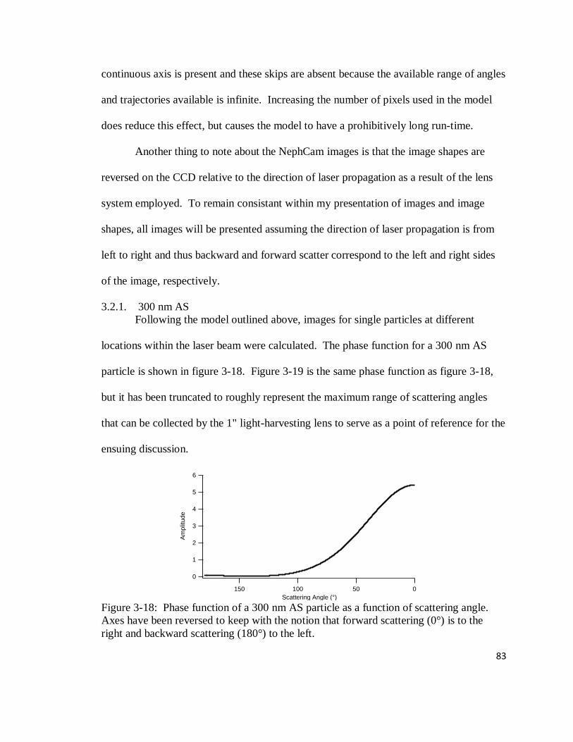
83
continuous axis is present and these skips are absent because the available range of angles
and trajectories available is infinite. Increasing the number of pixels used in the model
does reduce this effect, but causes the model to have a prohibitively long run-time.
Another thing to note about the NephCam images is that the image shapes are
reversed on the CCD relative to the direction of laser propagation as a result of the lens
system employed. To remain consistant within my presentation of images and image
shapes, all images will be presented assuming the direction of laser propagation is from
left to right and thus backward and forward scatter correspond to the left and right sides
of the image, respectively.
3.2.1. 300 nm AS
Following the model outlined above, images for single particles at different
locations within the laser beam were calculated. The phase function for a 300 nm AS
particle is shown in figure 3-18. Figure 3-19 is the same phase function as figure 3-18,
but it has been truncated to roughly represent the maximum range of scattering angles
that can be collected by the 1" light-harvesting lens to serve as a point of reference for the
ensuing discussion.
Figure 3-18: Phase function of a 300 nm AS particle as a function of scattering angle.
Axes have been reversed to keep with the notion that forward scattering (0°) is to the
right and backward scattering (180°) to the left.
6
5
4
3
2
1
0
Am
plit
ude
150 100 50 0
Scattering Angle (°)

84
Figure 3-19: Truncated phase function to represent the maximum range of scattered
angles collected by the 1" light-harvesting lens.
The intersection angle (α0) of the scattered radiation and the focusing lens as a
function of scattering angle and particle position along the x-axis is shown in figure 3-20;
x-axis locations correspond to -418 (black), 0 (red) and +418 (purple) pixels. The
locations of these particles in the physical setup are shown with the same colors in figure
3-17. These locations represent a particle behind camera center, at camera center and a
particle forward of camera center. As the scattering angle reaches the limits of the
collection range the value of α0 approaches 90°. Figure 3-21, shows the values of cos(α0)
as a function of scattering angle (θ). This cos(α0) term represents the relative weighting
that must be applied to the phase function for the collection efficiency of the 1" light-
harvesting lens. When scattering angle is near 90°, collection efficiency is a maximum
(1) and quickly decreases towards 0 as the limit of collected scattering is approached.
The maximum collection efficiency shifts from angles greater than 90° to angles less than
90° as the particle location shifts forward in the camera's image.
2.0
1.5
1.0
0.5
0.0A
mplit
ude
120 110 100 90 80 70 60
Scattering Angle (°)

85
Figure 3-20: Angle of intersection of light scattered by a particle with an x pixel location
of 0 with the 1" focusing lens.
Figure 3-21: Cosine weight factor for scattered radiation by a particle at x pixel location
of 0.
When the cos(α0) weighting is applied to the phase function in figure 3-19, the
phase function's shape changes; minimum intensity now occurs at the image's edges. As
particle location shifts from behind center to forward of center, the range of scattering
angles collected also shifts towards the forward direction as shown in figures 3-22 and 3-
23. Figure 3-22 is the amplitude as a function of scattering angle and figure 3-23 is the
amplitude as a function of light harvesting lens pixel. The 2 curves show the same
information, but the trends are slightly different as a result of lens curvature. In figure 3-
23, it is important to note that depending upon whether the aerosol particle is behind or in
front of image center the collected amplitude reaches 0 in the forward and backward
directions, respectively, as a result of the cos(α0) weighting.
80
60
40
20
0
alp
ha
0
120 110 100 90 80 70 60
Scattering Angle (°)
x = -418 x = 0 x = 418
1.0
0.8
0.6
0.4
0.2
0.0
cos(a
lpha
0)
120 110 100 90 80 70 60
Scattering Angle (°)
x = -418 x = 0 x = 418

86
The phase function transmitted through the 1" light-harvesting lens is then
translated upwards through the CCTV lens to the CCD. Since the CCD is smaller than
both the light-harvesting lens and the CCTV lens, additional truncation of the phase
function is observed as a result of the angle of departure (β2) of the scattered ray from the
focusing lens. The resulting truncated amplitude distribution as a function of scattering
angle that reaches the CCD is shown in figure 3-24, for an aerosol particle behind center
(black), center (red) and forward of center (purple). Translating these scattering angles to
physical pixels on the CCD results in figure 3-25.
Figure 3-22: Intensity of scattered radiation being transmitted by the focusing lens as a
function of scattering angle.
Figure 3-23: Intensity of scattered radiation being transmitted by the focusing lens as a
function of point along the 1" light-harvesting lens.
0.6
0.4
0.2
0.0
Am
plit
ude
120 110 100 90 80 70 60
Scattering Angle (°)
x = -418 x = 0 x = 418
0.6
0.4
0.2
0.0
Am
plit
ude
-2000 -1000 0 1000 2000
Focusing Lens Point (x)
x = -418 x = 0 x = 418
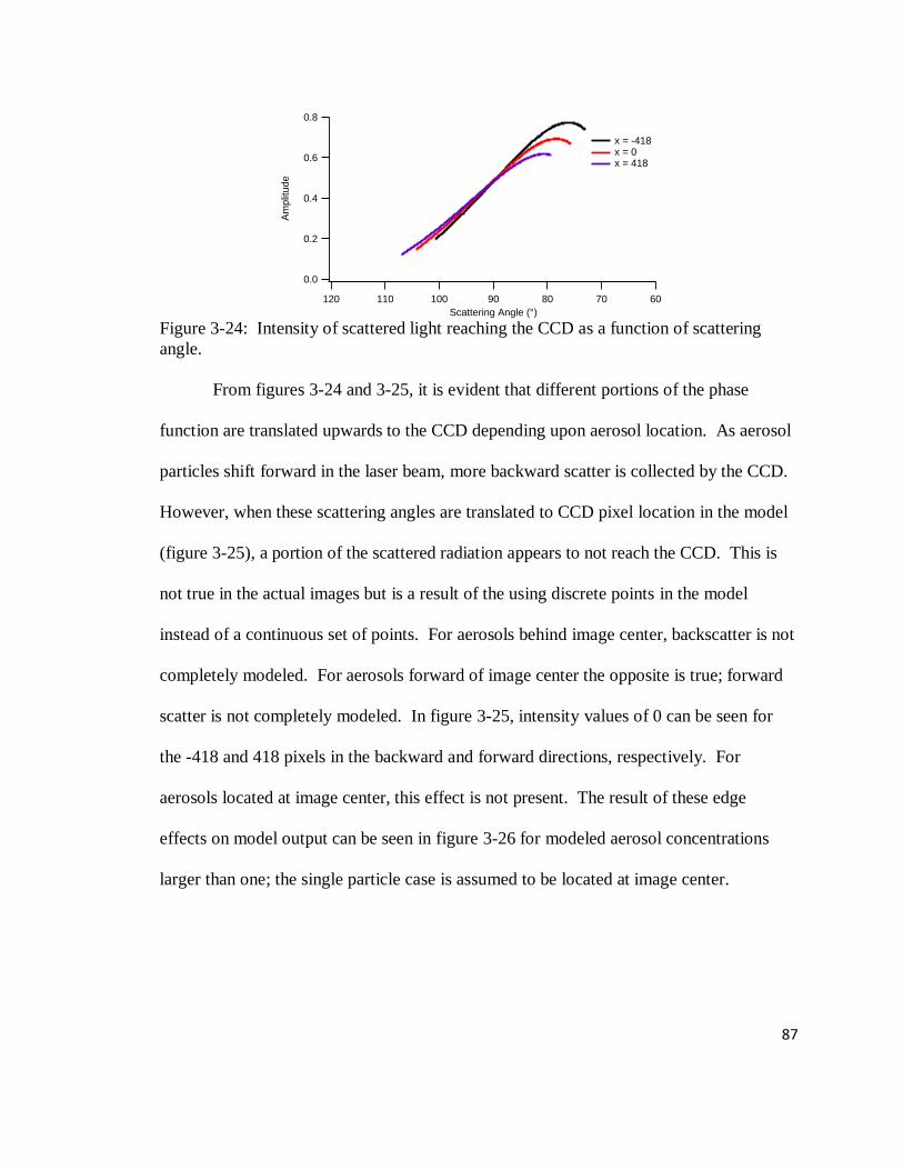
87
Figure 3-24: Intensity of scattered light reaching the CCD as a function of scattering
angle.
From figures 3-24 and 3-25, it is evident that different portions of the phase
function are translated upwards to the CCD depending upon aerosol location. As aerosol
particles shift forward in the laser beam, more backward scatter is collected by the CCD.
However, when these scattering angles are translated to CCD pixel location in the model
(figure 3-25), a portion of the scattered radiation appears to not reach the CCD. This is
not true in the actual images but is a result of the using discrete points in the model
instead of a continuous set of points. For aerosols behind image center, backscatter is not
completely modeled. For aerosols forward of image center the opposite is true; forward
scatter is not completely modeled. In figure 3-25, intensity values of 0 can be seen for
the -418 and 418 pixels in the backward and forward directions, respectively. For
aerosols located at image center, this effect is not present. The result of these edge
effects on model output can be seen in figure 3-26 for modeled aerosol concentrations
larger than one; the single particle case is assumed to be located at image center.
0.8
0.6
0.4
0.2
0.0A
mplit
ude
120 110 100 90 80 70 60
Scattering Angle (°)
x = -418 x = 0 x = 418

88
Figure 3-25: Intensity of scattered light reaching the CCD as a function of CCD pixel for
aerosols located at x pixels of -418 (black), 0 (red) and 418 (purple); pixel locations
relative to CCD shown in figure 1.
Figure 3-26: Normalized amplitudes of different model concentrations of 300 nm AS
aerosol: 1 particle (black), 10 particles (red), 100 particles (green) and 1000 particles
(blue).
Figure 3-27 below shows an actual average scattering image collected by the
NephCam. In comparing figures 3-26 and 3-27, images shapes are not very similar. This
discrepancy arises from two effects: the DMA sizing mechanism and NephCam MTF.
The DMA sizes particles based upon electrical mobility; similar ratios of charge to size
will have the same electrical mobility:
(eq 3-28)
where Z is the electrical mobility, q is the charge, dm is the equivalent mobility diameter
of an equivalent spherical particle and γ is a shape factor that accounts for slip and drag
0.6
0.4
0.2
0.0
Am
plit
ude
-600-400-2000200400600
CCD Pixel
x = -418 x = 0 x = 418
1.0
0.8
0.6
0.4
0.2
0.0
No
rma
lize
d A
mp
litu
de
120010008006004002000
Pixel
1 10 100 1000

89
inside of the DMA. Presently, γ was assumed to be 1.6. This value was chosen because
similar values have been used previously for coated soot particles; while AS is not
expected to have the same morphology as coated soot, it is not expected to be a
completely spherical particle either (Bueno, Havey et al. 2011). Calculated diameter
values for multiply charged particles assuming base diameter of 300 nm can be seen in
table 3-1. From these diameter values and the DMA's product literature, transmission
ratios as a function of size and charge were calculated for each size bin. These values
were then scaled to generate a discrete set of particles for modeling as seen in table 3-1
for 300 nm AS. Fractions of a particle were rounded to the nearest whole number since
only a whole number of particles can be modeled. The result of considering these
multiple size to charge effects can be seen in figure 3-28.
Figure 3-27: Actual average scattering image collected by the NephCam for 300 nm AS
aerosol
Table 3-1: Multiple charge to size particles and fraction for a 300 nm AS aerosol
Concentration at:
Diameter (nm) Charge Fraction 1 particle 10 particles 100 particles 1000 particles
300 1 0.744 1 7 74 744
463 2 0.170 0 2 17 170
596 3 0.059 0 1 6 59
714 4 0.018 0 0 2 18
820 5 0.007 0 0 1 7
919 6 0.002 0 0 0 2
1.0
0.8
0.6
0.4
0.2
0.0
No
rma
lize
d A
mp
litu
de
120010008006004002000
Pixel
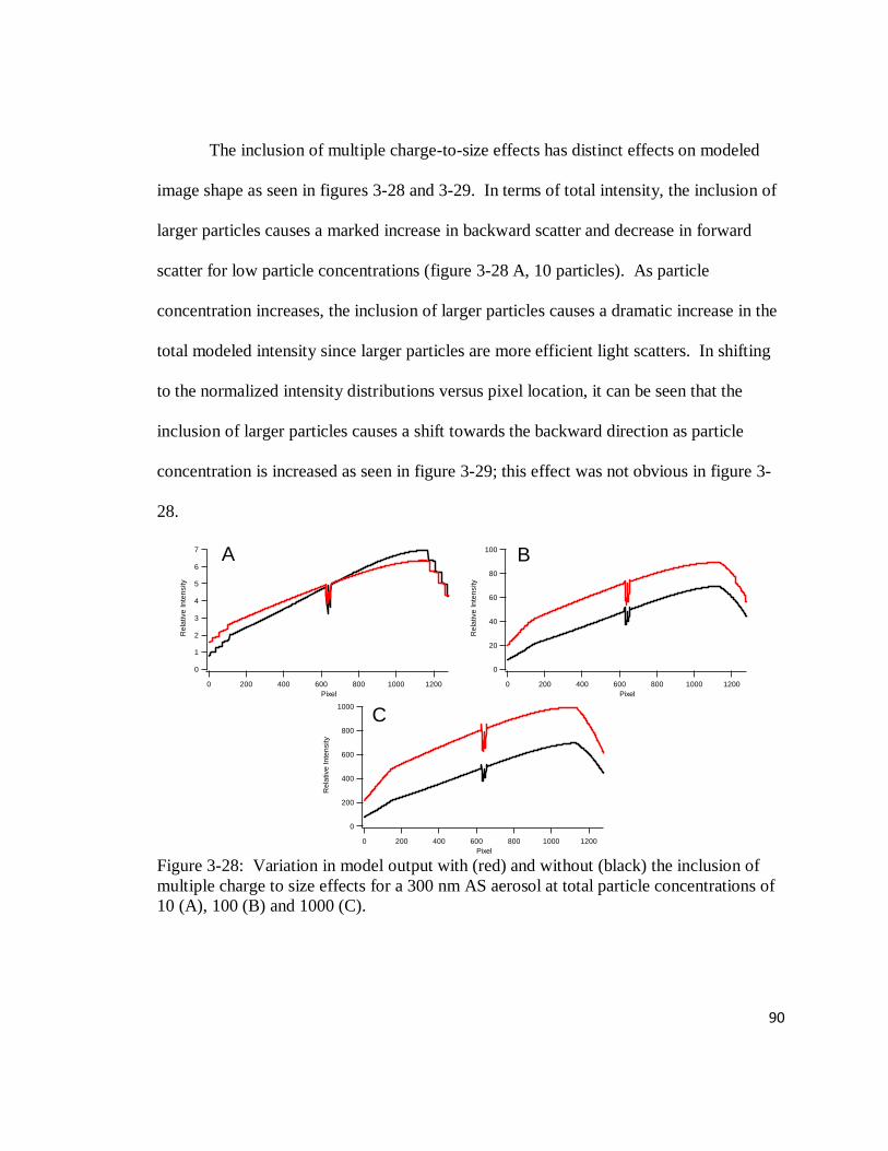
90
The inclusion of multiple charge-to-size effects has distinct effects on modeled
image shape as seen in figures 3-28 and 3-29. In terms of total intensity, the inclusion of
larger particles causes a marked increase in backward scatter and decrease in forward
scatter for low particle concentrations (figure 3-28 A, 10 particles). As particle
concentration increases, the inclusion of larger particles causes a dramatic increase in the
total modeled intensity since larger particles are more efficient light scatters. In shifting
to the normalized intensity distributions versus pixel location, it can be seen that the
inclusion of larger particles causes a shift towards the backward direction as particle
concentration is increased as seen in figure 3-29; this effect was not obvious in figure 3-
28.
Figure 3-28: Variation in model output with (red) and without (black) the inclusion of
multiple charge to size effects for a 300 nm AS aerosol at total particle concentrations of
10 (A), 100 (B) and 1000 (C).
7
6
5
4
3
2
1
0
Re
lative
In
ten
sity
120010008006004002000
Pixel
A 100
80
60
40
20
0
Re
lative
In
ten
sity
120010008006004002000
Pixel
B
1000
800
600
400
200
0
Re
lative
In
ten
sity
120010008006004002000
Pixel
C
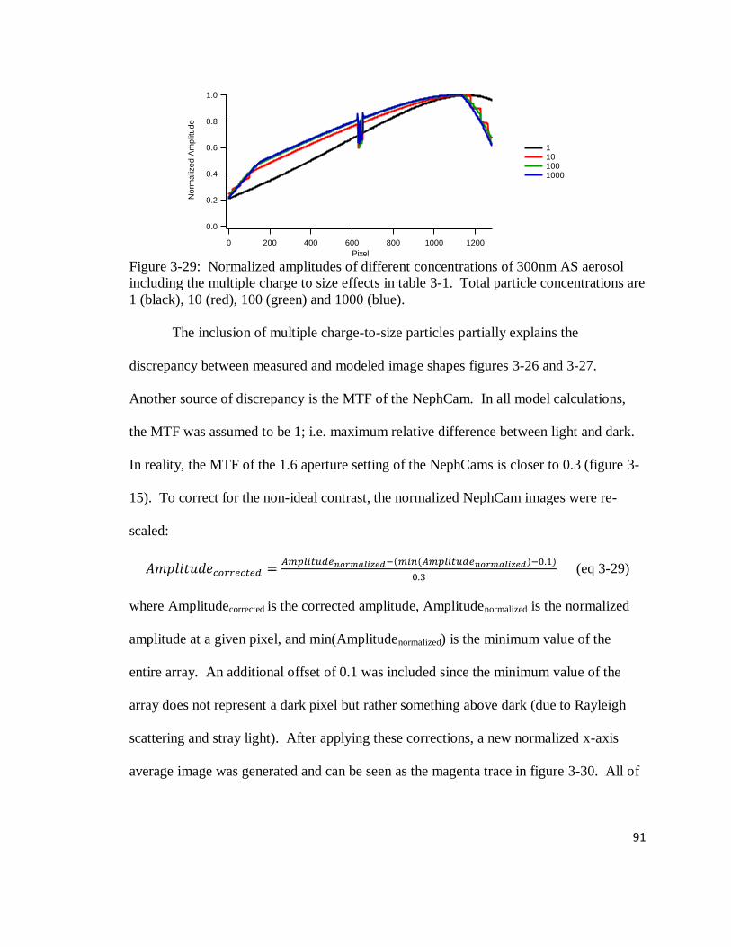
91
Figure 3-29: Normalized amplitudes of different concentrations of 300nm AS aerosol
including the multiple charge to size effects in table 3-1. Total particle concentrations are
1 (black), 10 (red), 100 (green) and 1000 (blue).
The inclusion of multiple charge-to-size particles partially explains the
discrepancy between measured and modeled image shapes figures 3-26 and 3-27.
Another source of discrepancy is the MTF of the NephCam. In all model calculations,
the MTF was assumed to be 1; i.e. maximum relative difference between light and dark.
In reality, the MTF of the 1.6 aperture setting of the NephCams is closer to 0.3 (figure 3-
15). To correct for the non-ideal contrast, the normalized NephCam images were re-
scaled:
(eq 3-29)
where Amplitudecorrected is the corrected amplitude, Amplitudenormalized is the normalized
amplitude at a given pixel, and min(Amplitudenormalized) is the minimum value of the
entire array. An additional offset of 0.1 was included since the minimum value of the
array does not represent a dark pixel but rather something above dark (due to Rayleigh
scattering and stray light). After applying these corrections, a new normalized x-axis
average image was generated and can be seen as the magenta trace in figure 3-30. All of
1.0
0.8
0.6
0.4
0.2
0.0
No
rma
lize
d A
mp
litu
de
120010008006004002000
Pixel
1 10 100 1000
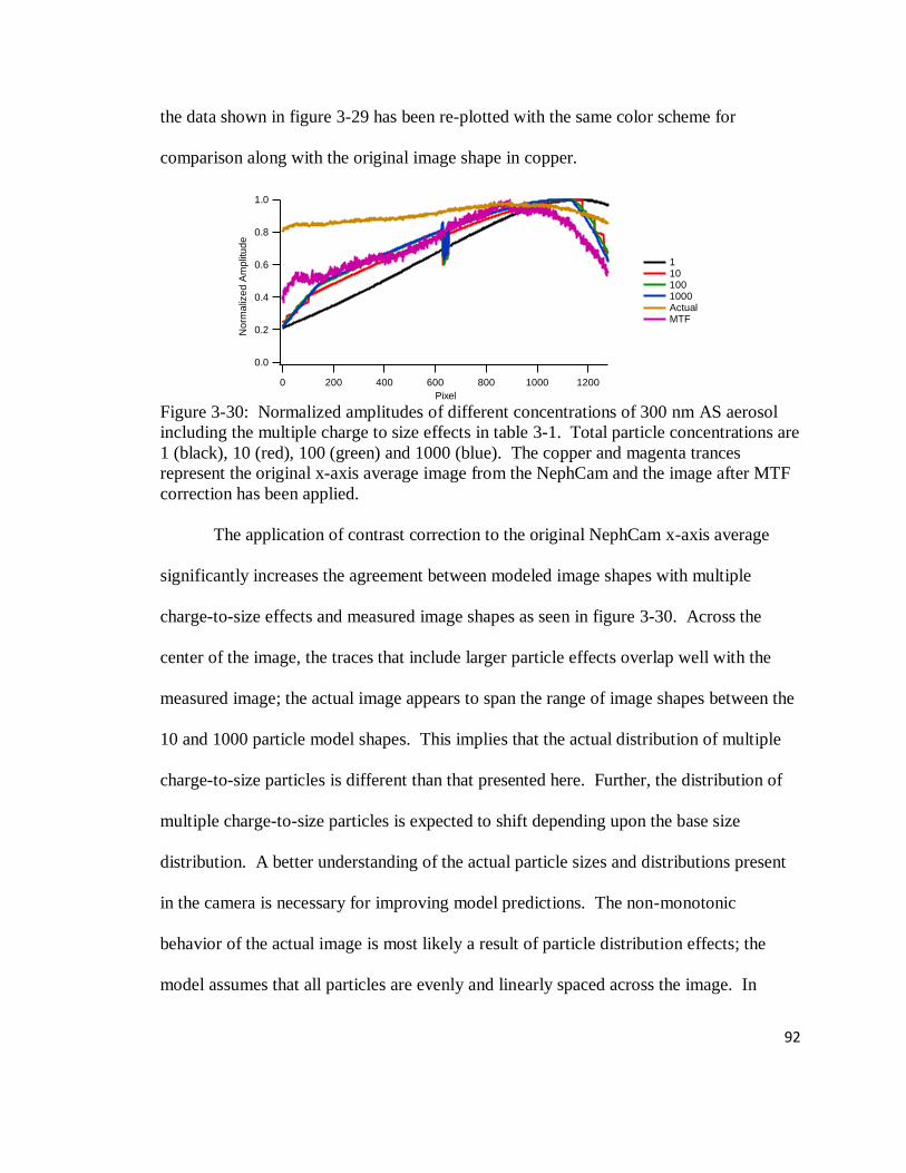
92
the data shown in figure 3-29 has been re-plotted with the same color scheme for
comparison along with the original image shape in copper.
Figure 3-30: Normalized amplitudes of different concentrations of 300 nm AS aerosol
including the multiple charge to size effects in table 3-1. Total particle concentrations are
1 (black), 10 (red), 100 (green) and 1000 (blue). The copper and magenta trances
represent the original x-axis average image from the NephCam and the image after MTF
correction has been applied.
The application of contrast correction to the original NephCam x-axis average
significantly increases the agreement between modeled image shapes with multiple
charge-to-size effects and measured image shapes as seen in figure 3-30. Across the
center of the image, the traces that include larger particle effects overlap well with the
measured image; the actual image appears to span the range of image shapes between the
10 and 1000 particle model shapes. This implies that the actual distribution of multiple
charge-to-size particles is different than that presented here. Further, the distribution of
multiple charge-to-size particles is expected to shift depending upon the base size
distribution. A better understanding of the actual particle sizes and distributions present
in the camera is necessary for improving model predictions. The non-monotonic
behavior of the actual image is most likely a result of particle distribution effects; the
model assumes that all particles are evenly and linearly spaced across the image. In
1.0
0.8
0.6
0.4
0.2
0.0
No
rma
lize
d A
mp
litu
de
120010008006004002000
Pixel
1 10 100 1000 Actual MTF
93
reality, this spacing is probably not accurate and instead a random or statistical
distribution of particles within the image beam should be used. In the backward scatter
and forward scatter directions (approaching pixels 0 and 1240, respectively), the
measured and modeled images do not agree as well, but this is probably due to improper
characterization of edge effects in the model.
3.2.2. 100 nm AS
Similar trends are seen for other AS particle sizes; the 100 nm case is shown
below. In figure 3-31, normalized image shapes for 100 nm AS - with multiplets - at
concentrations of 10 (red), 100(green) and 1000 (blue) are shown. The 1 particle case
has been omitted because the normalized amplitude for a single particle at 100 nm is a
flat line at 1.0; model output is only 3 decimal places and higher precision is required for
these values. However, the actual model does operate using more significant digits. In
table 3-2, the particle sizes included as multiplets and their modeled concentrations are
shown. Again, image shape agreement between the actual image and the model improves
after the MTF has been applied (Contrast, magenta). Good agreement between the actual
image and the model is also obtained, but this arises from the fact that 100 nm particles
have a phase function that is very symmetric in all directions. Agreement could be
further improved by including a 306 nm particle in the model calculations; it was not
included because the probability of obtaining a particle of 306 nm with a +6 charge is
essentially 0 (larger particles are more accommodating to higher charges).

94
Figure 3-31: Normalized model amplitudes for a 100 nm AS aerosol with multiplets
assuming 10 (red), 100 (green) and 1000 (blue) aerosol particles. Actual image shape is
shown in copper and the corrected image shape after MTF correction has been applied.
Table 3-2: Multiple charge to size particles and fraction for a 100nm AS aerosol
Concentration at:
Diameter (nm) Charge Fraction 10 particles 100 particles 1000 particles
100 1 0.8469 8 85 847
154 2 0.1259 1 13 126
199 3 0.0227 0 2 23
238 4 0.0035 0 0 4
273 5 0.0006 0 0 1
306 6 0.0005 0 0 0
3.2.3. 700 nm AS
The modeled and measured image shapes for 700 nm AS particles are shown in
figure 3-32 for 1 (black), 10 (red), 100 (green) and 1000 (blue) particles. The actual
image obtained by the camera is shown in copper and the image after contrast correction
in magenta. Only single size particles (no multiplets) were modeled for this size bin; the
1μm impactor on the SMPS prevents the 1.080μm +2 particle from getting through to the
camera. Agreement between the modeled and measured image shapes is again improved
after the contrast correction but is not as good as the smaller particle sizes. This is most
likely a result of single particle effects. The measured extinction during the 700 nm
experiments was approximately 45 Mm-1
which translates to roughly 30 particles/cc in
1.0
0.8
0.6
0.4
0.2
0.0
No
rma
lize
d A
mp
litu
de
120010008006004002000
Pixel
10 100 1000 Actual MTF
multi size

95
the extinction measurement and only 1 particle being imaged at any given moment in
time. For the smaller particle sizes, the number concentration of particles was
significantly higher (greater than 1,000/cc). Thus, the linear spacing of particles within
the laser beam may not be as appropriate for the larger size as the smaller size.
Figure 3-32: Normalized model amplitudes for a 700 nm AS aerosol assuming 10 (red),
100 (green) and 1000 (blue) aerosol particles. Actual image shape is shown in copper
and the corrected image shape after MTF correction has been applied. Multiplets are not
included in these calculations.
3.3. Calibration slopes as a function of particle size
The image shapes generated from the model were also used to simulate
calibration curves for the NephCam as a function of size. In processing the actual
NephCam images for scattering intensity, averages across the horizontal axis of the
image are taken and then the resulting curve is fit to a Lorentzian; peak amplitude
corresponds to scattering intensity. However, the model developed only uses a single
axis; so the average intensity across a simulated image was used as a surrogate for peak
amplitude. Also, the model operates by calculating the image shape as a function of an
aerosol distribution present in the laser beam over an undetermined amount of time and
all calculated intensities are based upon a relative intensity calculated using Mie Theory.
1.0
0.8
0.6
0.4
0.2
0.0
No
rma
lize
d A
mp
litu
de
120010008006004002000
Pixel
1 10 100 1000 Actual MTF
96
Thus these simulated images cannot be directly linked to any given exposure length, but
the trends seen in the simulated images can be applied to the NephCam data.
Particle size affects both the image shapes (as shown above) and the calibration
curves for the NephCam. In keeping with the trends noticed in the image shape
calculations, the effect of multiple charge-to-size particles were included here. Figures 3-
33 and 3-34 show modeled calibration curves for 100 nm and 500 nm AS aerosols,
respectively. In figure 3-33 the calibration curve is noticeably non-linear as a result of
larger particle effects in the calculated images and scattering values. This non-linearity is
represented as a negative parabolic term in the calibration curve. As particle size is
increased, these non-linear effects from multiple charge-to-size particles decreases; the
modeled calibration curve for 500 nm AS in figure 3-34 appears linear. These trends can
be seen for the NephCam AS data in figures 3-35 and 3-36 for 100 nm and 500 nm,
respectively. One major difference between the modeled and actual 100 nm AS data is
the magnitude of downward curvature. This arises because the model must assume a
discrete number of aerosol "pixels" to model while the actual images represent a
continuous measurement of particles in time.
The decrease in negative parabolic curvature with size arises because the relative
change in total scattering by multiplets decreases with increasing particle size. In the
case of 100 nm particles, the 154 nm, 199 nm, 238 nm 273 nm and 306 nm multiplets are
12, 52, 126, 253 and 468 times as efficient at scattering as the 100 nm particle. For a 500
nm particle, a 771 nm particle is only 2.5 times more efficient. So, while the 500 nm
particles might show some negative parabolic curvature, it is going to be much less than
for the 100 nm particle. For particles 700 nm and larger, multiplets are not present
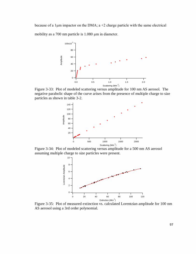
97
because of a 1μm impactor on the DMA; a +2 charge particle with the same electrical
mobility as a 700 nm particle is 1.080 μm in diameter.
Figure 3-33: Plot of modeled scattering versus amplitude for 100 nm AS aerosol. The
negative parabolic shape of the curve arises from the presence of multiple charge to size
particles as shown in table 3-2.
Figure 3-34: Plot of modeled scattering versus amplitude for a 500 nm AS aerosol
assuming multiple charge to size particles were present.
Figure 3-35: Plot of measured extinction vs. calculated Lorentzian amplitude for 100 nm
AS aerosol using a 3rd order polynomial.
100x10-3
80
60
40
20
0
Am
plit
ud
e
2.01.51.00.50.0
Scattering (Mm-1
)
140
120
100
80
60
40
20
Am
plit
ud
e
2000150010005000
Scattering (Mm-1
)
10
8
6
4
2
0
Lo
ren
tzia
n A
mp
litu
de
120100806040200
Extinction (Mm-1
)
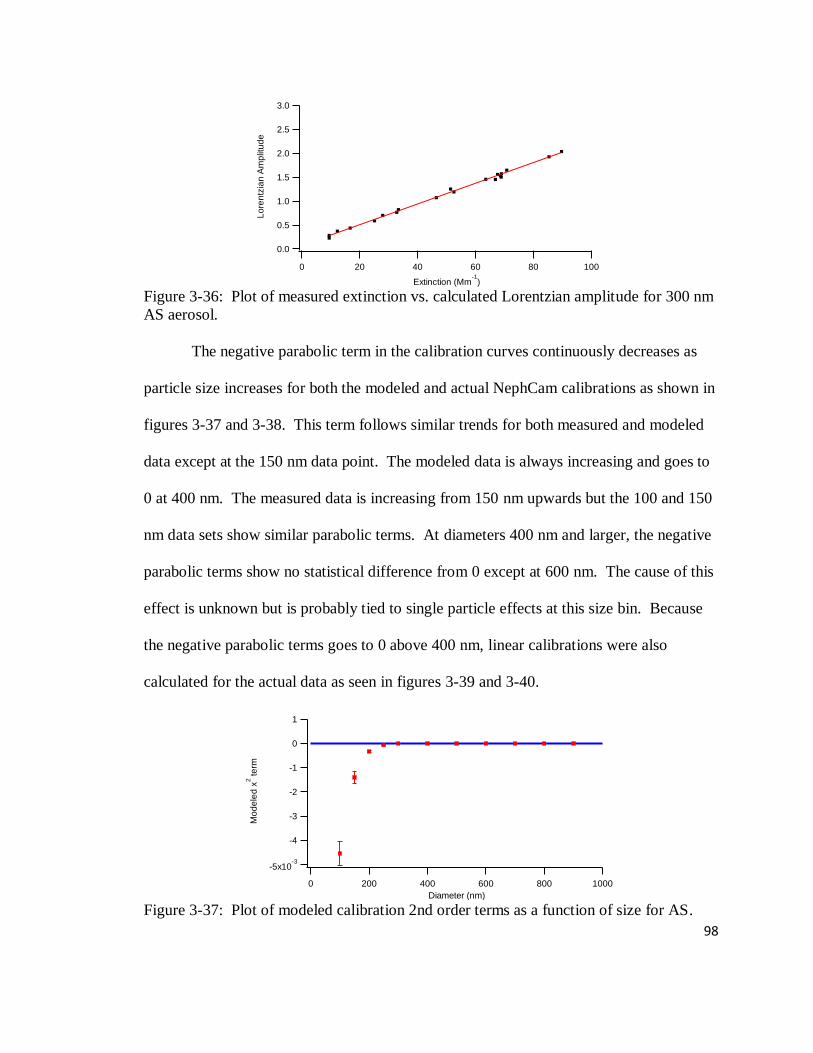
98
Figure 3-36: Plot of measured extinction vs. calculated Lorentzian amplitude for 300 nm
AS aerosol.
The negative parabolic term in the calibration curves continuously decreases as
particle size increases for both the modeled and actual NephCam calibrations as shown in
figures 3-37 and 3-38. This term follows similar trends for both measured and modeled
data except at the 150 nm data point. The modeled data is always increasing and goes to
0 at 400 nm. The measured data is increasing from 150 nm upwards but the 100 and 150
nm data sets show similar parabolic terms. At diameters 400 nm and larger, the negative
parabolic terms show no statistical difference from 0 except at 600 nm. The cause of this
effect is unknown but is probably tied to single particle effects at this size bin. Because
the negative parabolic terms goes to 0 above 400 nm, linear calibrations were also
calculated for the actual data as seen in figures 3-39 and 3-40.
Figure 3-37: Plot of modeled calibration 2nd order terms as a function of size for AS.
3.0
2.5
2.0
1.5
1.0
0.5
0.0
Lo
ren
tzia
n A
mp
litu
de
100806040200
Extinction (Mm-1
)
-5x10⁻³
-4
-3
-2
-1
0
1
Mo
de
led
x2 te
rm
10008006004002000
Diameter (nm)
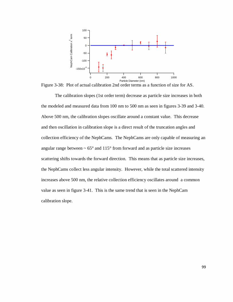
99
Figure 3-38: Plot of actual calibration 2nd order terms as a function of size for AS.
The calibration slopes (1st order term) decrease as particle size increases in both
the modeled and measured data from 100 nm to 500 nm as seen in figures 3-39 and 3-40.
Above 500 nm, the calibration slopes oscillate around a constant value. This decrease
and then oscillation in calibration slope is a direct result of the truncation angles and
collection efficiency of the NephCams. The NephCams are only capable of measuring an
angular range between ~ 65° and 115° from forward and as particle size increases
scattering shifts towards the forward direction. This means that as particle size increases,
the NephCams collect less angular intensity. However, while the total scattered intensity
increases above 500 nm, the relative collection efficiency oscillates around a common
value as seen in figure 3-41. This is the same trend that is seen in the NephCam
calibration slope.
-150x10-6
-100
-50
0
50
100
Ne
ph
Ca
m C
alib
ratio
n x
2 te
rm
10008006004002000
Particle Diameter (nm)

100
Figure 3-39: Plot of modeled calibration 1st order term as a function of size for AS using
linear (black dots) and polynomial fits (red squares).
Figure 3-40: Plot of actual calibration 1st order term as a function of size for AS using
linear (black dots) and polynomial fits (red squares).
The modeled and measured NephCam calibration intercepts do not show any
definitive trends. In the modeled data, the intercepts oscillate around 0 as seen in figure
3-42. This is probably a result of the set of particles and the ratio of different particle
sizes chosen for the model. If different collections of particles had been modeled then the
intercepts might go towards 0. In the measured calibration intercepts, figure 3-43, many
of the polynomial fits show little statistical difference from 0. However, at smaller
particle sizes the intercepts for the linear calibration fits are statistically different from 0.
0.4
0.3
0.2
0.1
0.0
Mo
de
led
Ca
libra
tio
n S
lop
e
10008006004002000
Diameter (nm)
Linear Polynomial
0.10
0.08
0.06
0.04
0.02
0.00
Ne
ph
Ca
m C
alib
ratio
n S
lop
e
10008006004002000
Particle Diameter (nm)
Linear Polynomial

101
Figure 3-41: Plot of NephCam scattering collection versus total scattering (collection
efficiency) as a function of size for AS particles.
Figure 3-42: Plot of modeled calibration intercepts as a function of size for AS using
linear (black dots) and polynomial fits (red squares).
Figure 3-43: Plot of actual calibration intercepts as a function of size for AS using linear
(black dots) and polynomial fits (red squares).
After modeling and physically determining the NephCam calibration slope, the
NephCams were used to determine the scattering coefficients of Nigrosin aerosol. These
coefficients were then compared to measured extinction values from the HC-CRDT so
15
10
5
0C
olle
ctio
n E
ffic
ien
cy (
%)
10008006004002000
Diameter (nm)
0.8
0.6
0.4
0.2
0.0
-0.2
-0.4
-0.6
Mo
de
led
Ca
libra
tio
n In
terc
ep
t
10008006004002000
Diameter (nm)
Linear Polynomial
0.8
0.6
0.4
0.2
0.0
-0.2
Am
bie
nt-
A N
ep
hC
am
C
alib
ratio
n In
terc
ep
t
10008006004002000
Particle Diameter (nm)
Linear Polynomial
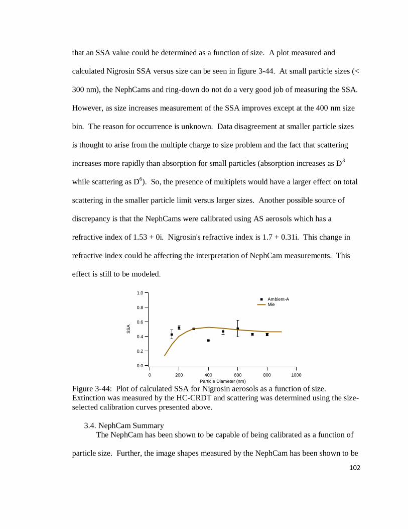
102
that an SSA value could be determined as a function of size. A plot measured and
calculated Nigrosin SSA versus size can be seen in figure 3-44. At small particle sizes (<
300 nm), the NephCams and ring-down do not do a very good job of measuring the SSA.
However, as size increases measurement of the SSA improves except at the 400 nm size
bin. The reason for occurrence is unknown. Data disagreement at smaller particle sizes
is thought to arise from the multiple charge to size problem and the fact that scattering
increases more rapidly than absorption for small particles (absorption increases as D3
while scattering as D6). So, the presence of multiplets would have a larger effect on total
scattering in the smaller particle limit versus larger sizes. Another possible source of
discrepancy is that the NephCams were calibrated using AS aerosols which has a
refractive index of 1.53 + 0i. Nigrosin's refractive index is 1.7 + 0.31i. This change in
refractive index could be affecting the interpretation of NephCam measurements. This
effect is still to be modeled.
Figure 3-44: Plot of calculated SSA for Nigrosin aerosols as a function of size.
Extinction was measured by the HC-CRDT and scattering was determined using the size-
selected calibration curves presented above.
3.4. NephCam Summary
The NephCam has been shown to be capable of being calibrated as a function of
particle size. Further, the image shapes measured by the NephCam has been shown to be
1.0
0.8
0.6
0.4
0.2
0.0
SS
A
10008006004002000
Particle Diameter (nm)
Ambient-A Mie

103
related to the modeled image shape for AS aerosols as a function of size once contrast
effects and the sizing mechanism of the DMA are considered (multiple size to charge
effects). The SSA of an absorbing aerosol has been calculated using the HC-CRDT as an
extinction measurement. The inversion of the NephCam measurement from any arbitrary
image shape to determine average particle size and scattering is still a work in progress.
Further modeling and measurements of aerosols with known properties need to be
conducted. However, in going forward, there are some specific details that need to be
addressed:
A sizing mechanism that completely removes the multiple charge to size effect
needs to be used. Many of the modeling studies were forced to assume things about the
size distributions that may or may not have been true in reality. Addressing whether
these assumptions were actually justified is required.
The width of the aerosol sample within the NephCam body needs to be decreased.
Currently, a 1/2" Cu tube is expanded to a 1" tube at the inlet of the NephCam. This
allows for slight diffusional broadening of the aerosol sample within the body of the
NephCam. Instead, the size of the flow should be stepped down so that the imaged width
of aerosols is less than the width of the image in the NephCam. This would prevent
multiply scattered rays that originated outside of the camera's imaging area from reaching
the detector. The exit side of the NephCam can be left at the current size since this
doesn't have any effect on the images.
Another detector(s) needs to be added to the NephCam. Specifically, a detector
situated in the forward direction is necessary. This would allow the NephCam an
additional piece of information when trying to extract information about particle size,

104
shape and total scattering intensity. Right now, because particle size is known, the
truncation angle error can be corrected. In the event that particle size is not known this
error cannot be corrected. The addition of another detector in the backwards direction
would give even more information about the shape function of the aerosol under
investigation. Particle sizing by DLS for nano-particles is typically done at 7° off of
forward. Incorporating a similar of measurement may facilitate the extraction of size
information of aerosols under investigation.
A beam splitter with a detector to measure laser intensity in real time is required.
Currently, laser intensity is inferred from polynomial background gray fits. However, the
laser stability may be less than what is currently inferred from the polynomial fits.
Having a real time measurement of laser intensity in time will allow for better
characterization of laser amplitude and the actual intensity of the scattering measurement.
The speed of data collection needs to be addressed. Currently, the triggering and
subsequent data collection is limited by the semaphore control of the camera drivers.
Realistically, faster images need to be taken to optimize the intensity and size information
obtained. However, depending upon the exact magnitude of scattering towards the
camera sensor by particles dictates the minimum exposure time allowable. When only
large particles are present, the cameras can be operated in a free-run video mode for real
time capturing of scattering coefficients. However, under most circumstances the total
scattering by particles and light directed towards the CCD is less than minimum amount
detectable by the CCD in video capture mode (15 fps). Optimization of the camera setup
may allow for the NephCam to be run in a video collection mode at lower than maximum
frame rates (~ 1 fps) for real time determination of scattering and image shape. To use

105
this type of video (instead of image collection) an individual computer is necessary for
each camera. Hard drive and RAM installed on each computer is another issue (i.e. at 15
fps, video requires ~ 1 MB per second and the RAM to support a live video feed).
Image contrast needs to be reassessed. Under the current setup, a decision
between maximum contrast and constant contrast across an image had to be made. The
choice was to go with constant contrast across an image. However, in making this choice
changes in image intensity had to be inferred (see equation 3-29) relative to some "dark"
value and it was only marginally better than unusable (0.3 vs. 0.2, respectively). But, it
was possible to make measured and modeled image shapes agree by inferring a contrast
difference between the models (which assume perfect contrast) and the measured images.
106
4. Results & Discussion - Humidification experiments
4.1. Allan Variance
Allan Variance experiments are conducted to determine the optimal integration
length for minimum noise in a measurement. To perform this Allan Variance, the HC-
CRDT was allowed to sample clean air for 4 days (96 hours). An Allan Variance plot
can be seen in figure 4-1 for the visible on the Humidified channel. Raw ring-down data
as a function of data points is the red trace at the top. The computed Allan Variance is
the black trace below that as a function of integration time. The lighter gray trace
represents the theoretical variance if only white noise was present. The computed Allan
variance initially follows the gray trace which decreases as √N. After approximately 200
data points (13 seconds) the theoretical and actual variance start to deviate and the
variance starts increasing after 1600 data points (107 seconds) due to instrumental drift.
Only one channel is shown since similar plots were generated for each channel and
wavelength.
Allan variance is also reported as an Allan Deviation - variance equals standard
deviation squared. This corresponds to the maximum precision in any measurement.
Calculated Allan Deviations for each channel and wavelength of the HC-CRDT are
shown in table 4-1 as a function of integration time. Values for the Ambient-B IR
channel have been omitted since that channel is non-functional. As the integration length
is increased, the deviation does decrease for the IR and UV channels. In the visible and
the UV of the Humidified channel, the minimum deviation is obtained at 120 seconds and
increases minimally in going from 120 to 240 seconds. As a result, 240 seconds was
chosen as the optimal integration time as it did represent the minimum deviation for
many of the channels.

107
Figure 4-1: Allan variance plot for the visible on the Humidified channel. Red data at
the top of the figure is the actual ring-down data as a function of data points. Dark black
trace at the bottom shows actual variance as a function of integration time in points on a
logarithmic scale. Light gray trace is the ideal variance as a function of integration time
if only white noise was present.
Table 4-1: Allan deviation results as a function of integration time for the HC-CRDT
Seconds Pulses Channel IR (±Mm-1
) Vis (±Mm-1) UV (±Mm-1)
1 15
Ambient-A 5.73 0.57 4.98
Ambient-B -- 1.11 21.52
Dry 9.80 1.91 8.98
Humidified 3.63 0.44 12.59
60 900
Ambient-A 0.75 0.27 1.12
Ambient-B -- 0.36 2.87
Dry 1.27 0.42 1.31
Humidified 0.48 0.10 2.49
120 1800
Ambient-A 0.57 0.24 0.93
Ambient-B -- 0.40 2.00
Dry 0.90 0.38 0.98
Humidified 0.36 0.09 2.03
240 3600
Ambient-A 0.51 0.26 0.96
Ambient-B -- 0.51 1.50
Dry 0.66 0.41 0.86
Humidified 0.28 0.11 2.12

108
4.2. Characterizing direct sums fitting routine
The direct sums fitting routine has been previously shown to have good accuracy
and precision when extracting ring-down coefficients at a ring-down time of 1.5μsec and
a Gaussian noise level of 1% (Everest and Atkinson 2008). However, in fitting raw data
obtained by the CRD, these values are highly dependent on the base ring-down time and
the noise encountered. Figure 4-2 shows the precision of the direct sums fitting routine
for 3600 fits (240 seconds) assuming 1% (black) and 10% (red) periodic random noise in
a simulated ring-down signal at various extinction levels. As the base extinction
increases, the precision decreases and is always worse than that calculated by the Allan
variance. For extinction levels above 3000 Mm-1
this implies that measurement errors are
directly linked to the fitting routine not converging on the correct value.
Figure 4-2: Precision of 3600 simulated ring-down fits using the direct sums algorithm
as a function of the actual extinction assuming that periodic random noise at 1% and 10%
levels.
4.3. Characterizing HC-CRDT transmission efficiency without Humidity controls
In switching from the size-selected experiments to the humidity controlled
experiments, the aerosol delivery system was rearranged. For these experiments,
aerosols were sampled directly through a URG-2000-30EQ cyclone into a mixing
chamber and the DMA was operated in parallel to the HC-CRDT. (In the size selected
100
80
60
40
20
0
Pre
cis
ion
of fits
(± M
m-1
)
40003000200010000
Actual Extinction (Mm-1
)
1% Noise 10% Noise
109
experiments, the DMA was in series with the 2nd mixing chamber and HC-CRDT
providing particle size selection before measurement.) Here, well-characterized full size
distributions were desired instead of a single particle size, hence the change in
configuration.
In the visible, agreement with the Ambient-A channel was within 10% for the Dry
and Humidified channels (without the dryer and humidifier) and within 20% for the
Ambient-B channel, which is within instrument precision. In the IR agreement was not
as good but this was not surprising because the extinction in the IR was very near the
LOQ for all channels. Higher extinction values would have been desirable, but this
causes the UV extinction coefficients to be prohibitively high for measurement. In the
UV, good agreement (< 1%) of the Ambient-B channel and the dry (< 12%) and
humidified (< 16%) channels with the Ambient-A channel was obtained . Unlike the
Visible channel, some of the UV values did not agree to within instrument precision, so
minor correction factors were applied to this data.
4.4. Humidifier and dryer particle transmission
To compare the effects of humidity on particle optical properties, it was necessary
to first correct for the incomplete transmission of particles through the humidifier and
dryer. Particle transmission data for the 20 ppm AS and 20 ppm Nigrosin were similar, so
only figures for the AS will be shown. Figures 4-3, 4-4, and 4-5 show the results of the
particle transmission testing experiments in the absence of the humidifier or dryer, with
only the dryer and with only the humidifier, respectively. The number of particles
counted upstream of the dryer and humidifier by the CPC3007 is approximately constant
across all experiments. The downstream particle concentration obtained from the

110
CPC3776 changes in each experiment but is always higher than the number counted by
the CPC3007. This is not unexpected because of the lower minimum size detected by the
CPC3776, and can still allow a transmission loss measurement if the "no dryer or
humidifier" case is taken as the basis for comparison.
Figure 4-3: Time series data of 20 ppm AS particle transmission testing without
humidifier or dryer present. Three cycles of measurement, interspersed with filtered air
measurements, are shown.
Figure 4-4: Time series of 20 ppm AS particle transmission testing with dryer.
Figure 4-5: Time series data for 20 ppm AS particle transmission testing with humidifier.
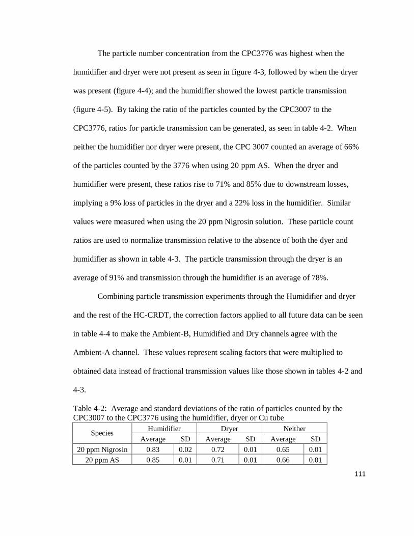
111
The particle number concentration from the CPC3776 was highest when the
humidifier and dryer were not present as seen in figure 4-3, followed by when the dryer
was present (figure 4-4); and the humidifier showed the lowest particle transmission
(figure 4-5). By taking the ratio of the particles counted by the CPC3007 to the
CPC3776, ratios for particle transmission can be generated, as seen in table 4-2. When
neither the humidifier nor dryer were present, the CPC 3007 counted an average of 66%
of the particles counted by the 3776 when using 20 ppm AS. When the dryer and
humidifier were present, these ratios rise to 71% and 85% due to downstream losses,
implying a 9% loss of particles in the dryer and a 22% loss in the humidifier. Similar
values were measured when using the 20 ppm Nigrosin solution. These particle count
ratios are used to normalize transmission relative to the absence of both the dyer and
humidifier as shown in table 4-3. The particle transmission through the dryer is an
average of 91% and transmission through the humidifier is an average of 78%.
Combining particle transmission experiments through the Humidifier and dryer
and the rest of the HC-CRDT, the correction factors applied to all future data can be seen
in table 4-4 to make the Ambient-B, Humidified and Dry channels agree with the
Ambient-A channel. These values represent scaling factors that were multiplied to
obtained data instead of fractional transmission values like those shown in tables 4-2 and
4-3.
Table 4-2: Average and standard deviations of the ratio of particles counted by the
CPC3007 to the CPC3776 using the humidifier, dryer or Cu tube
Species Humidifier Dryer Neither
Average SD Average SD Average SD
20 ppm Nigrosin 0.83 0.02 0.72 0.01 0.65 0.01
20 ppm AS 0.85 0.01 0.71 0.01 0.66 0.01
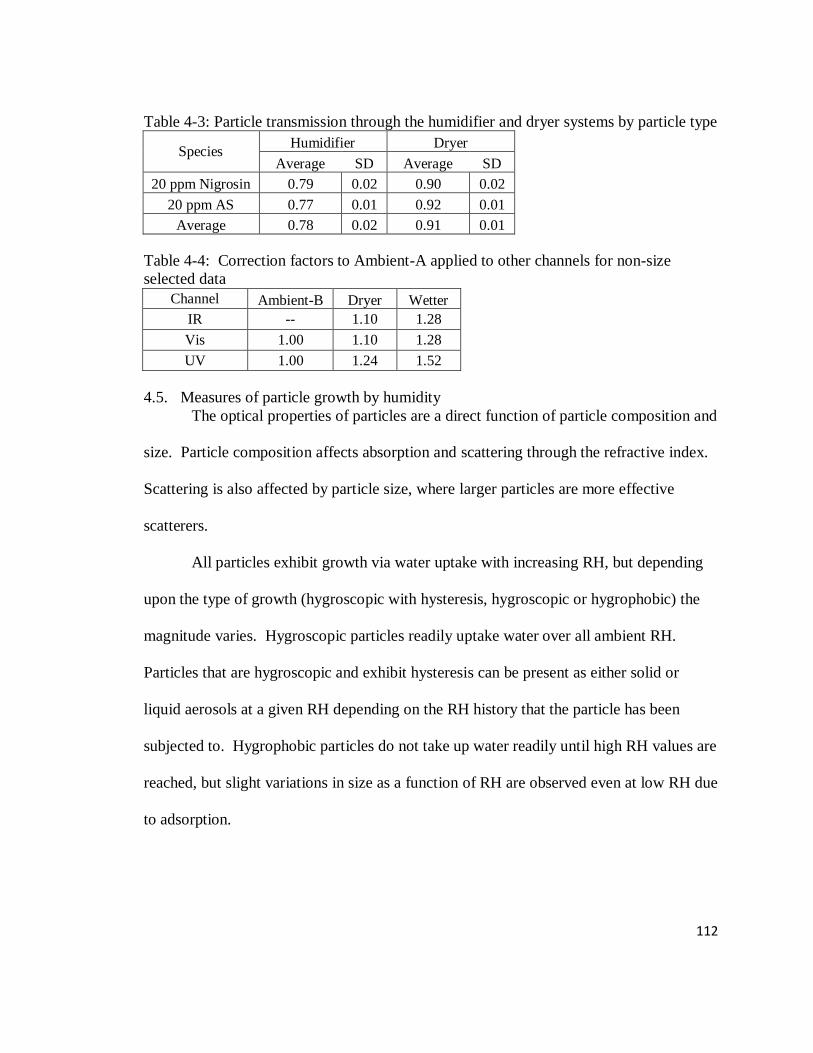
112
Table 4-3: Particle transmission through the humidifier and dryer systems by particle type
Species Humidifier Dryer
Average SD Average SD
20 ppm Nigrosin 0.79 0.02 0.90 0.02
20 ppm AS 0.77 0.01 0.92 0.01
Average 0.78 0.02 0.91 0.01
Table 4-4: Correction factors to Ambient-A applied to other channels for non-size
selected data
Channel Ambient-B Dryer Wetter
IR -- 1.10 1.28
Vis 1.00 1.10 1.28
UV 1.00 1.24 1.52
4.5. Measures of particle growth by humidity
The optical properties of particles are a direct function of particle composition and
size. Particle composition affects absorption and scattering through the refractive index.
Scattering is also affected by particle size, where larger particles are more effective
scatterers.
All particles exhibit growth via water uptake with increasing RH, but depending
upon the type of growth (hygroscopic with hysteresis, hygroscopic or hygrophobic) the
magnitude varies. Hygroscopic particles readily uptake water over all ambient RH.
Particles that are hygroscopic and exhibit hysteresis can be present as either solid or
liquid aerosols at a given RH depending on the RH history that the particle has been
subjected to. Hygrophobic particles do not take up water readily until high RH values are
reached, but slight variations in size as a function of RH are observed even at low RH due
to adsorption.
113
There are different parameters that are alternatively used to describe droplet
growth as a function of RH. The simplest, droplet growth factors (β) are the ratio of
particle size at an elevated RH to dry particle size:
(eq 4-1)
where D is the particle diameter at elevated RH and D0 is the dry particle diameter. The
measurement of β commonly uses a Tandem Differential Mobility Analyzer (TDMA)
instrument. In these experiments, only the change in diameter of particles is of interest
and experiments measuring the change in particle diameter as a function of water uptake,
organic uptake, or simply SOA growth have been performed in a similar manner with this
instrument (Gysel, Weingartner et al. 2001; Stanier, Pathak et al. 2007; Lewis, Arnott et
al. 2009). From the experiments reported in this work, β can only be inferred since the
HC-CRDT is an optical measurement. Instead, f(RH) and γ(RH) are the commonly
applied measures of particle growth:
(eq 4-2)
where bext(dry) and bext(RH) are the extinction coefficients of an ensemble of aerosol
particles at dry and ambient RH. In many cases the dry RH is taken to be any RH less
than 40% (Baltensperger, Barrie et al. 2003). As will be shown below, this value is not
low enough to consider some types of particles "dry" for the purposes of determining
f(RH). For many efflorescent salts an RH less than 40% is acceptable. For some salts
(e.g., NaNO3) and hygroscopic aerosols not exhibiting efflorescence or hygrophobic
aerosols it is not.

114
The values of f(RH) have been modeled well by equation 4-3 for aerosols
showing monotonic growth and hygroscopicity:
(eq 4-3)
Where a and b are parameters obtained from a non-linear curve fitting procedure
(Carrico, Kus et al. 2003; Pan, Yan et al. 2009). The form of f(RH) for hydrated
hygroscopic aerosols that exhibit efflorescence and deliquescence has been modeled by:
(eq 4-4)
where c and g are also model fit parameters. This last f(RH) function has been used
repeatedly to describe the RH dependence of ambient aerosols, regardless of whether the
aerosol demonstrates deliquescence behavior or not (Kotchenruther, Hobbs et al. 1999;
Carrico, Kus et al. 2003). Depending upon the measurements available, f(RH) can
instead be expressed as γ(RH):
(eq 4-5)
(eq 4-6)
where bext(RH) and bext(dry) are the extinction coefficients at high and low RH,
respectively, and RHhigh and RHdry are the measured relative humidities (%). Identical
expressions can be composed for the scattering and absorption effects of RH, but the
application to scattering is more common than absorption since the change in scattering
with RH is larger and more systematic than that of absorption. The application of γ(RH)
is similar to that of the Ångström exponent in that it simulates an assumed power law
dependence of extinction on RH (instead of wavelength).

115
The relative humidity growth factor γ(RH) in equations 4-5 and 4-6 is essentially
the same as g in equation 4-4, since γ(RH) can be derived from g by taking the
logarithmic derivative of equation 4-4. Both f(RH) and γ(RH) contain similar
information, but the measurement context is slightly different. Proper measurement of
f(RH) requires the ability to cycle RH and collect "humidograms", time dependent
measurements of the aerosol optical properties that are synchronized to the RH
dependence. Pair-wise f(RH) values can be calculated as long the optical properties are
measured at 2 or more RH's but less information is provided. The measurement of
humidograms allows for the elucidation of hysteretic behavior in aerosol growth because
the RH is cycled between high and low extremes and efflorescence and deliquescence
can be directly observed. The disadvantage is that obtaining humidograms is time-
consuming; typically 30 minutes or more are required for a single loop, and the aerosol
composition and concentration should optimally remain constant for this whole period.
Because it assumes a form for the growth of particles with RH, the measurement
of γ(RH) only requires measurement of optical properties at 2 or more relative
humidities. In this approach, parallel measurements of the various RH-dependent
properties (e.g., extinction coefficients) are usually made, generally in real time. When
the property is measured at 3 or more RH values (high, medium , dry), pair-wise values
for γ(RH) from equation 4-6 will be similar for both pairs (medium to high RH and
medium to low RH) when hysteresis is not present. In this case, a non-linear fit can be
used to obtain γ(RH) from equation 4-5 using as many measurements as are available. If
a hysteretic aerosol is present and the low RH is below the efflorescence RH, then γ(RH)

116
will have different values for each γ(RH) pair present, indicating that the non-linear fit
would not be applicable.
While f(RH) and γ(RH) represent the integral versus differential effect of RH on
particle growth respectively, both conventions will be used in my presentation of data
collected. The HC-CRDT is usually used to measure γ(RH) but is also able to obtain
humidograms and thus f(RH); f(RH) will be the preferred form when linking measured
data to model results. The γ(RH) will be preferred when only diagnostic information is
desired.
4.6. Changes in refractive index due to water uptake
Global climate models use effective refractive indices to predict the radiative
forcing of aerosols (Bond and Bergstrom 2006). In many cases, the base refractive index
used in the calculation is inferred based upon a given particle type - scattering salts, black
carbon, brown carbon, etc. These base refractive indices are typically an
oversimplification to other types of aerosol actually present (mixed organics, coated
organics, core-shell type particles, mixed salt and organics) and particles are typically
assumed to be spherical for ease of calculation using Mie theory. The assumption of
spherecity may be justified when averaging over a large enough ensemble of particles,
but the effects of particle composition cannot be ignored. The change in refractive index
with relative humidity is inferred from different refractive index mixing rules, including
the volume mixing, Maxwell-Garnett, and partial molar refraction models described in
the next sections. As a result, the radiative forcing predictions of GCM's by aerosols as a
function of RH give variable results that may or may not even correspond to what is
actually present and occurring in the atmosphere. Improvement in the understanding of
117
particle refractive indices (and therefore optical properties) as a function of RH is of
importance for better simulations of aerosol radiative forcing in global climate models.
4.6.1. Water uptake and dilution effects on particle refractive index
Water uptake by particles with increasing humidity alters the inherent optical
properties of the particle (approaching those of water) through changes in composition,
morphology and structure. If dry particle size is known, then changes in particle size are
attributable to the adsorption or absorption of water and the resulting particle composition
can be calculated. The refractive index and optical properties of the hydrated particle can
then be calculated by assuming the particle is spherical and homogeneous. Not
accounting for refractive index changes with water uptake can result in an overestimation
of the optical properties; as a result the inferred radiative forcing by the particle takes on
significant error and my even be of the wrong sign/direction (Erlick, Abbatt et al. 2011).
4.6.1.1. Volume mixing
Refractive index mixing rules represent an approximation to the solution of
Maxwell's equations for particles of mixed composition either as a result of formation
mechanisms or water uptake. The simplest of these mixing rules, the volume mixing
rule, states that the effective refractive index of a particle is simply a function of the
volume fractions of the species present:
(eq 4-7)
where neff is the effective index of the particle and fi and ni are the volume fraction and
bulk refractive index of species i. The real and imaginary terms of the effective refractive
index are calculated separately. The volume mixing rule is an oversimplification of the
actual refractive index of an inhomogeneous particle but is useful because of its
118
simplicity and ability to account for any number of aerosol components (Erlick, Abbatt et
al. 2011).
4.6.1.2. Maxwell-Garnett
The Maxwell-Garnett (MG) mixing rule is typically applied to particles with
absorbing inclusions in a non-absorbing bulk where the inclusions are small relative to
the size of the particle. Here, the MG mixing rule will be applied to all particles of mixed
composition regardless of whether the inclusions are absorbing. The MG mixing rule is
based on changes in the dielectric constant of a particle with inclusions:
(eq 4-8)
where ϵeff is the effective dielectric constant, f is the volume fraction of the inclusions and
ϵinclusion and ϵparticle are the dielectric constants of the inclusions and the particle matrix,
respectively. The dielectric constant (ϵ) is related to the refractive index (n) by:
(eq 4-9)
This mixing rule can be extended to any particle of mixed composition if only a single
type of inclusion is present in an otherwise homogeneous particle (Chyýlek, Srivastava et
al. 1988).
The MG mixing rule assumes that the inclusions are non-interacting, spherical
and randomly distributed within the particle. Second-order effects of interactions by
inclusions within a particle are ignored. The MG mixing rule can be expanded into
different forms if the inclusions are not spherical but needles, oblate or prolate discs, or
other defined shapes (Bohren and Huffman 1983; Sihvola 2008). However, for the salts
and organics investigated in this work these other forms are not necessary because all
119
particle types investigated are water soluble. One of the major drawbacks to the MG
mixing rule is that only a single type of inclusion can be considered when calculating the
effective refractive index.
4.6.1.3. Partial molar refraction
In the partial molar refraction mixing rule, the effective refractive index of a
particle is based upon the volume mixing of all species present and their molar
refractions. The molar refraction (R) of a species is:
(eq 4-10)
Where n is the complex refractive index and V, the molar volume, is:
(eq 4-11)
where MW is the molecular weight of the species and ρ is the density. Once the molar
refractions of the individual species are known, the effective molar refraction of a
mixture (Reff) is:
(eq 4-12)
Where xi is the mole fraction of species i and Ri is the molar refraction of species i. The
effective molar volume of a mixture (Veff) is:
(eq 4-13)
where xi is the mole fraction of species i, MWi is the molecular weight of species i and ρi
is the density of species i. The effective refractive index of the particle can then be
calculated by re-arranging equation 4-10, to solve for n:
120
(eq 4-14)
In (Stelson 1990), the partial molar refraction was only applied to real refractive indices.
Since eq 4-14 can be derived from eq 7 by a simple algebraic rearrangement, it should
then follow that this equation is also applicable to refractive indices with imaginary
components.
The partial molar refraction mixing rule assumes that all components within the
mixture are ideal; no 2nd order interactions between the species are present . The partial
molar refraction mixing rule has the advantage that multiple components can be included
as with the volume mixing rule.
4.6.2. RF inaccuracies from refractive index changes
The volume, partial molar refraction and MG mixing rules give similar results in
the determination of the real part of the refractive index for a test aerosol, as seen in
figure 4-6. However, these three mixing rules give significantly different values for the
imaginary refractive index as seen in figure 4-7. The volume mixing rule gives the
highest imaginary refractive index, while the MG rule has an imaginary refractive index
that is an average of 10% lower and a partial molar refraction that is an average of 14%
lower.
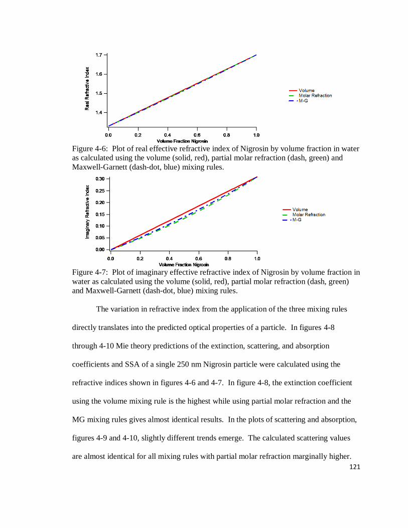
121
Figure 4-6: Plot of real effective refractive index of Nigrosin by volume fraction in water
as calculated using the volume (solid, red), partial molar refraction (dash, green) and
Maxwell-Garnett (dash-dot, blue) mixing rules.
Figure 4-7: Plot of imaginary effective refractive index of Nigrosin by volume fraction in
water as calculated using the volume (solid, red), partial molar refraction (dash, green)
and Maxwell-Garnett (dash-dot, blue) mixing rules.
The variation in refractive index from the application of the three mixing rules
directly translates into the predicted optical properties of a particle. In figures 4-8
through 4-10 Mie theory predictions of the extinction, scattering, and absorption
coefficients and SSA of a single 250 nm Nigrosin particle were calculated using the
refractive indices shown in figures 4-6 and 4-7. In figure 4-8, the extinction coefficient
using the volume mixing rule is the highest while using partial molar refraction and the
MG mixing rules gives almost identical results. In the plots of scattering and absorption,
figures 4-9 and 4-10, slightly different trends emerge. The calculated scattering values
are almost identical for all mixing rules with partial molar refraction marginally higher.
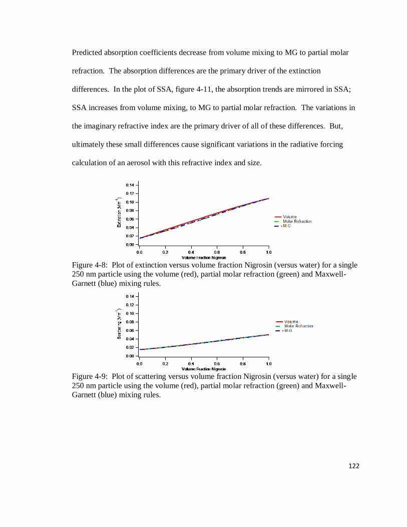
122
Predicted absorption coefficients decrease from volume mixing to MG to partial molar
refraction. The absorption differences are the primary driver of the extinction
differences. In the plot of SSA, figure 4-11, the absorption trends are mirrored in SSA;
SSA increases from volume mixing, to MG to partial molar refraction. The variations in
the imaginary refractive index are the primary driver of all of these differences. But,
ultimately these small differences cause significant variations in the radiative forcing
calculation of an aerosol with this refractive index and size.
Figure 4-8: Plot of extinction versus volume fraction Nigrosin (versus water) for a single
250 nm particle using the volume (red), partial molar refraction (green) and Maxwell-
Garnett (blue) mixing rules.
Figure 4-9: Plot of scattering versus volume fraction Nigrosin (versus water) for a single
250 nm particle using the volume (red), partial molar refraction (green) and Maxwell-
Garnett (blue) mixing rules.
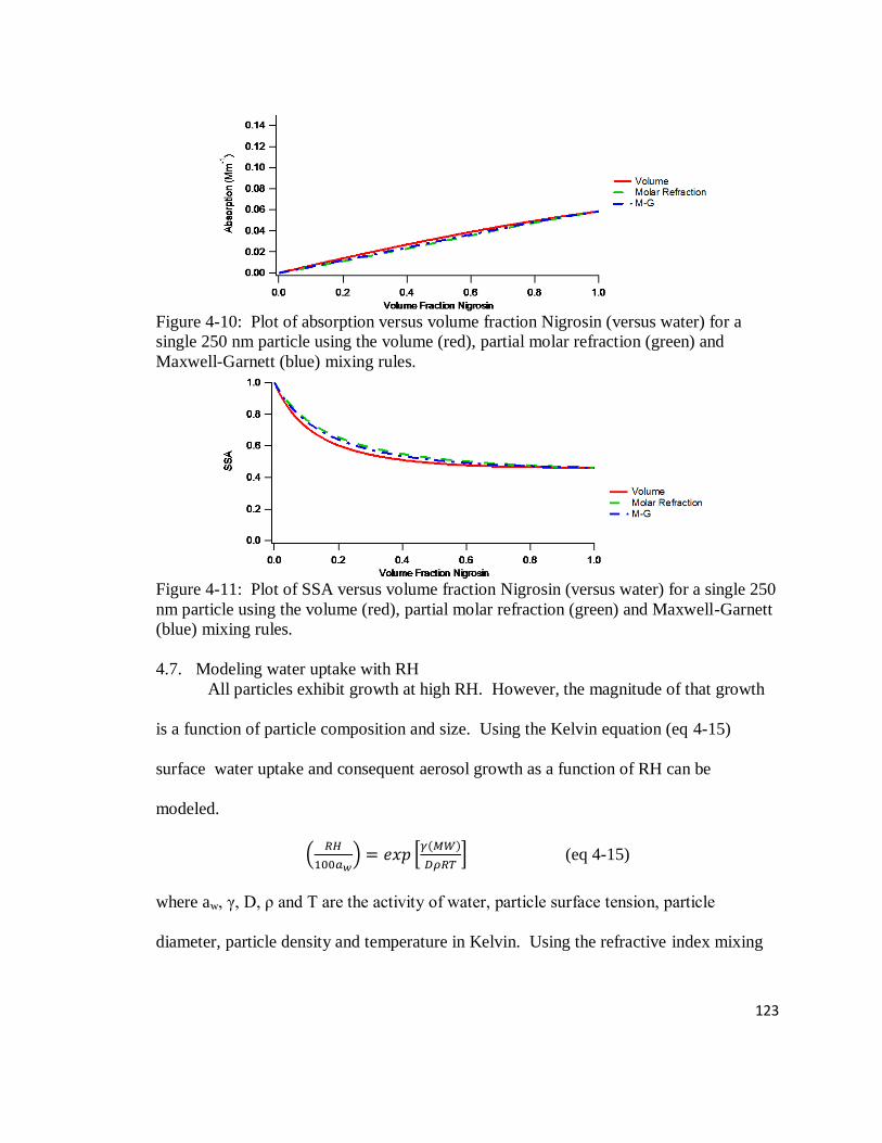
123
Figure 4-10: Plot of absorption versus volume fraction Nigrosin (versus water) for a
single 250 nm particle using the volume (red), partial molar refraction (green) and
Maxwell-Garnett (blue) mixing rules.
Figure 4-11: Plot of SSA versus volume fraction Nigrosin (versus water) for a single 250
nm particle using the volume (red), partial molar refraction (green) and Maxwell-Garnett
(blue) mixing rules.
4.7. Modeling water uptake with RH
All particles exhibit growth at high RH. However, the magnitude of that growth
is a function of particle composition and size. Using the Kelvin equation (eq 4-15)
surface water uptake and consequent aerosol growth as a function of RH can be
modeled.
(eq 4-15)
where aw, γ, D, ρ and T are the activity of water, particle surface tension, particle
diameter, particle density and temperature in Kelvin. Using the refractive index mixing

124
rules outlined above, the optical properties as a result of this growth can also be
calculated.
4.7.1. Inputs
4.7.1.1. Refractive Index
Table 4-5 shows the bulk refractive indices, molecular weights and ERH/DRH for
the species measured by the HC-CRDT and modeled here. The MW of Nigrosin was
taken as 202g/mole (from the Sigma Aldrich, Inc. product literature). Depending upon
supplier and source of Nigrosin, the MW has also been quoted as 616.49 g/mole. The
density of bulk Nigrosin was assumed to be 1 g/mL since a reference value could not be
found. The other model parameters of Nigrosin listed below were assumed to be the
same as NaNO3 since both exhibited similar growth characteristics and a literature value
was not available.
Table 4-5: Refractive indices, molecular weights, solid density and ERH/DRH for
modeled species from (Tang 1996)
Species n k MW (g/mole) Density (g/mL) ERH (%) DRH
(%)
NaNO3 1.587 0 84.9947 2.261 0.05 - 30 74.5
NaCl 1.55 0 58.44 2.165 46 - 48 75.3
NH4NO3 1.554 0 80.052 1.725 25 - 32 62
AS 1.53 0 132.14 1.76 37 - 40 80
Nigrosin 1.701 0.31 202 1 -- --
4.7.1.2. Density
For salt particles (sodium chloride, sodium nitrate, ammonium nitrate and
ammonium sulfate aerosols), density has been parameterized as a polynomial function of
weight percent salt in the particle (Tang and Munkelwitz 1994):
(eq 4-16)

125
where Ai is a fit parameter and x is the weight percent of the salt in the particle. In this
model, the density at 100% salt was taken as the actual salt density from table 4-5 instead
of the value calculated using eq 4-16. Values for these parameters of the species used in
this work can be seen in table 4-6.
Table 4-6: Fit parameters for eq 4-16 for modeled species density
Species Weight Percent Range A1 A2 A3 A4
NaNO3a
0 - 98 6.512x10⁻³
3.03x10⁻⁵
1.44x10⁻⁷
0
NaClb
-- 7.41x10⁻³
3.741x10⁻⁵
2.252x10⁻⁶ -2.06x10
-8
NH4NO3b
-- 4.05x10⁻³
9.0x10⁻⁶
1.024x10⁻⁸ 0
ASa
0 - 78 5.92x10⁻³
-5.036x10⁻⁶ 1.024x10
-8 0
Nigrosin -- 6.512x10⁻³
3.03x10⁻⁵
1.44x10⁻⁷
0
a (Tang and Munkelwitz 1994)
b (Tang 1996)
4.7.1.3. Activity
For salt particles, water activity has been parameterized as a polynomial function
of weight percent salt in the particle (Tang and Munkelwitz 1994):
(eq 4-17)
Where Ci is a fit parameter and x is the weight percent of the salt in the particle. Values
for these parameters can be seen in table 4-7.
Table 4-7: Activity fit parameters for eq 4-17 for modeled species
Species C1 C2 C3 C4
NaNO3a
-5.52x10⁻³
1.286x10⁻⁴
-3.496x10⁻⁶ 1.843x10
-8
NaClb
-6.366x10⁻³
8.624x10⁻⁵
-1.158x10⁻⁵ 1.518x10
-7
NH4NO3b
-3.65x10⁻³
-9.155x10⁻⁶
-2.826x10⁻⁷ 0
ASa
-2.715x10⁻³
3.113x10⁻⁵
-2.336x10⁻⁶ 1.412x10
-8
Nigrosin -5.52x10⁻³
1.286x10⁻⁴
-3.496x10⁻⁶ 1.843x10
-8
a (Tang and Munkelwitz 1994)
b (Tang 1996)

126
4.7.1.4. Surface tension
Surface tension is also a parameter in the Kelvin equation. For salt particles,
parameters to calculate the surface tension of a solution droplet of mixed composition
have been previously determined (Dutcher, Wexler et al. 2010). The surface tension
(ζ(T)) of a particle composed of salt and water is:
(eq 4-18)
Where ζw(T) and ζs(T) are the surface tension contributions from pure water and a
molten salt and yw and ys are the mole fractions of water and salt, respectively. The
surface tension contribution from water ζw(T) can be calculated from:
(eq 4-19)
Where T is the temperature in Kelvin and ζw(T) is in mN m-1
(or mJ m-2
). The surface
tension contribution of the molten salt ζs(T) can be calculated from:
(eq 4-20)
Where c1 and c2 are fit parameters and T is the temperature in Kelvin. Values for c1 and
c2 can be seen in table 4-8.
Table 4-8: Molten salt parameters for the calculation of surface tension, adapted from
(Dutcher, Wexler et al. 2010)
Species c1 (mN m-1
) c2 (mN m-1
K-1)
NaNO3 155.5 -0.0613
NaCl 191.16 -0.07188
NH4NO3 148.4 -0.105
AS 228.5 -0.146
Nigrosin 155.5 -0.0613
The terms ζw(T) and ζs(T) can be expanded to account for concentration effects at
high water and salt concentrations. At high water concentrations, salt ions can be thought

127
of as being solvated by water forming hydration shells. For water, the ζw(T) term can be
expanded:
(eq 4-21)
Where aws and bws are parameters fitted to the data. The same expansion can be done for
salt:
(eq 4-22)
Where asw and bsw are parameters fitted to the data. In the limit of high salt
concentration, the water droplets can be thought of as being solvated by salt ions; i.e. the
salt has a regular structure (Dutcher, Wexler et al. 2010). The order of subscripts in this
system is important: the left subscript indicates the high concentration species and right
subscript is the low concentration species. Values for aws, bws, asw and bsw can be found
in table 4-9 (taken from (Dutcher, Wexler et al. 2010)).
Table 4-9: High concentration limit solution and salt parameters for the calculation of
surface tension
Species aws (mN m-1
) bws (mN m-1
K-1
) asw (mN m-1
) bsw (mN m-1
K-1
)
NaNO3 19.359 0 0 0
NaCl 232.54 -0.245 -142.2 0
NH4NO3 -24.245 0.14 0 0
AS 0 0.366 0 -0.289
Nigrosin 19.359 0 0 0
Rewriting equation 4-17 to include equations 4-21 and 4-22 allows calculation of the
surface tension of the modeled particles:
(eq 4-23)

128
4.7.1.5. Size distribution data
In this work, the aerosol size distributions were determined by 2 methods: mean
diameters and geometric standard deviations were taken directly from the SMPS
(produced by the TSI Aerosol Instrument Manager software) and the same parameters
were calculated by fitting the raw size distributions (particle number concentration vs.
DMA diameter setpoint) using a log-normal curve. Further explanation is provided in
section 5.9.1. These base particle sizes were necessary to infer particle growth from that
on the Dry and Ambient channels to that on the Humidified channel as measurement of
particle size distributions at the RH of the Humidified channel were not possible using
the setup employed. From this growth, the optical properties of the Humidified channel
relative to the Dry and Ambient channels could be calculated.
4.7.1.6. RH
RH values for the SMPS were inferred from the measurements by the Ambient-A
RH/T sensor. This sensor was on a separate flow line in parallel to the SMPS, but the
time separation between the 2 measurements was minimal. The SMPS recirculates
excess flow as sheath flow so the actual value of the RH measured by the Ambient-A
channel could be slightly lower or higher than that in the SMPS depending upon whether
the ambient RH was decreasing or increasing, respectively.
4.7.2. Assumptions
There are four primary assumptions used in this model to calculate particle
growth as a function of relative humidity and to predict the resulting aerosol optical
properties: 1) particle growth as a function of relative humidity is controlled by the
Kelvin equation and the Köhler effect is negligible due to small particle size, 2)
temperature was constant at 293 K, 3) all measured particles are spherical and the optical
129
properties can be calculated using Mie theory and 4) all particles are completely
homogenous with respect to water; no core-shell morphologies are expected. These
assumptions are examined in greater detail in the next four paragraphs.
The assumption that particle growth is controlled by the Kelvin equation
ultimately serves as the basis for the calculation of particle diameter as a function of RH.
The measured geometric mean diameters for dry particles were typically in the range of
50 to 60 nm, except for NaNO3 which had a significantly smaller geometric mean
diameter near 25 nm. For particles in this size regime, the Kelvin equation serves as the
limiting case for particle growth. To assume that particles were able to freely grow in
this size range (as would be predicted without the Kelvin equation) results in significant
over predictions of growth and thus the optical properties. The RH of the humidified
channel was typically around 80 to 85% RH. For the types of particles measured here,
the Köhler effect is negligible since the humidified channel is not supersaturated with
water vapor (RH < 100%).
For the model calculations, the temperature was taken to be a constant value of
293K. In reality, the temperature of the lab varied between 290K and 295K, and small
temperature fluctuations were noticed during all experiments. In an absolute sense, the
temperature fluctuations were small (< 5 K), so it is not expected to affect modeling
results significantly.
Mie theory was used to calculate the optical properties of all particles for all RH.
Aerosol optical properties (extinction/scattering) were calculated using a LabView
adapted version of the C code written by Bohren and Huffman (1983); and modified by
130
Martin Fierz (Fierz 2005). Absorption was calculated from the difference between
extinction and scattering.
The assumption that Mie theory was applicable to all measured particles implies
that all of the particles were spherical at all RH's. Sodium chloride tends to effloresce
into a cubic shape as dictated by its crystal lattice, but for simplicity it was modeled as a
spherical homogeneous particle. This assumption also implies that the particles are either
completely mixed or a core-shell morphology of 2 homogeneous components. Mie
theory calculations can be performed on either morphology. However, the core-shell
morphology is not expected since all modeled particles are water soluble.
4.7.3. Model overview
Using the Kelvin equation (eq 4-15) and equations 4-16 through 4-23, the
equilibrium RH for a droplet with a defined mole fraction salt and water can be
calculated. This implies that the water activity and resulting equilibrium size can also be
predicted for a given RH. A plot of mole fraction water versus particle size and RH is
shown in figure 4-12, for AS aerosol. The 2 nm particle (solid black) has an ERH of
approximately 35%. This is where the mole fraction of the salt goes to 1. At any RH
below 35%, this particle would theoretically exist as a pure crystalline solid. However,
as particle size increases from 2 nm to 5 nm, the ERH drops significantly to around 20%.
As the particle continues to grow, ERH further decreases and approaches a limit around
10%. Although these calculations imply that an AS particle should effloresce around 10 -
15%, actual ERH is 37 - 40% (Tang 1996). This discrepancy is caused by the fact that
the difference in size between hydrated AS and crystalline AS near the ERH is small

131
compared to other types of salts (i.e. NaCl). As a result, a smooth but very gradual
increase in size is observed above 10% RH until the ERH is crossed.
Figure 4-12: Plot of % RH versus mole fraction AS for various particle diameters at
293K.
Using all of the parameters outlined above, particle growth as a function of RH
can be calculated as follows. A base size distribution at 0% RH is inferred from the
SMPS data and log-normal fits. At 0% RH, any particle type can be assumed to be in its
dry state (effloresced for most salts). The size distribution is initially assumed to have a
log-normal size distribution and is simulated as 1000 points evenly distributed between 1
nm and 1000 nm in log10 space. (Uniform increments in log space is the preferable way
to map the size distribution since this mirrors the way that the SMPS measures size
distributions.) Minimum size was limited to 1 nm because smaller particles do not
significantly affect the optical coefficients, even after being subjected to significant
growth. Maximum particle size was limited to 1000 nm to represent the size cut point of
the SMPS impactor and URG cyclone on the sampling line. From this base size
distribution, initial extinction and scattering coefficients are calculated using the Mie
code.
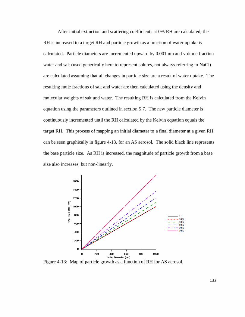
132
After initial extinction and scattering coefficients at 0% RH are calculated, the
RH is increased to a target RH and particle growth as a function of water uptake is
calculated. Particle diameters are incremented upward by 0.001 nm and volume fraction
water and salt (used generically here to represent solutes, not always referring to NaCl)
are calculated assuming that all changes in particle size are a result of water uptake. The
resulting mole fractions of salt and water are then calculated using the density and
molecular weights of salt and water. The resulting RH is calculated from the Kelvin
equation using the parameters outlined in section 5.7. The new particle diameter is
continuously incremented until the RH calculated by the Kelvin equation equals the
target RH. This process of mapping an initial diameter to a final diameter at a given RH
can be seen graphically in figure 4-13, for an AS aerosol. The solid black line represents
the base particle size. As RH is increased, the magnitude of particle growth from a base
size also increases, but non-linearly.
Figure 4-13: Map of particle growth as a function of RH for AS aerosol.
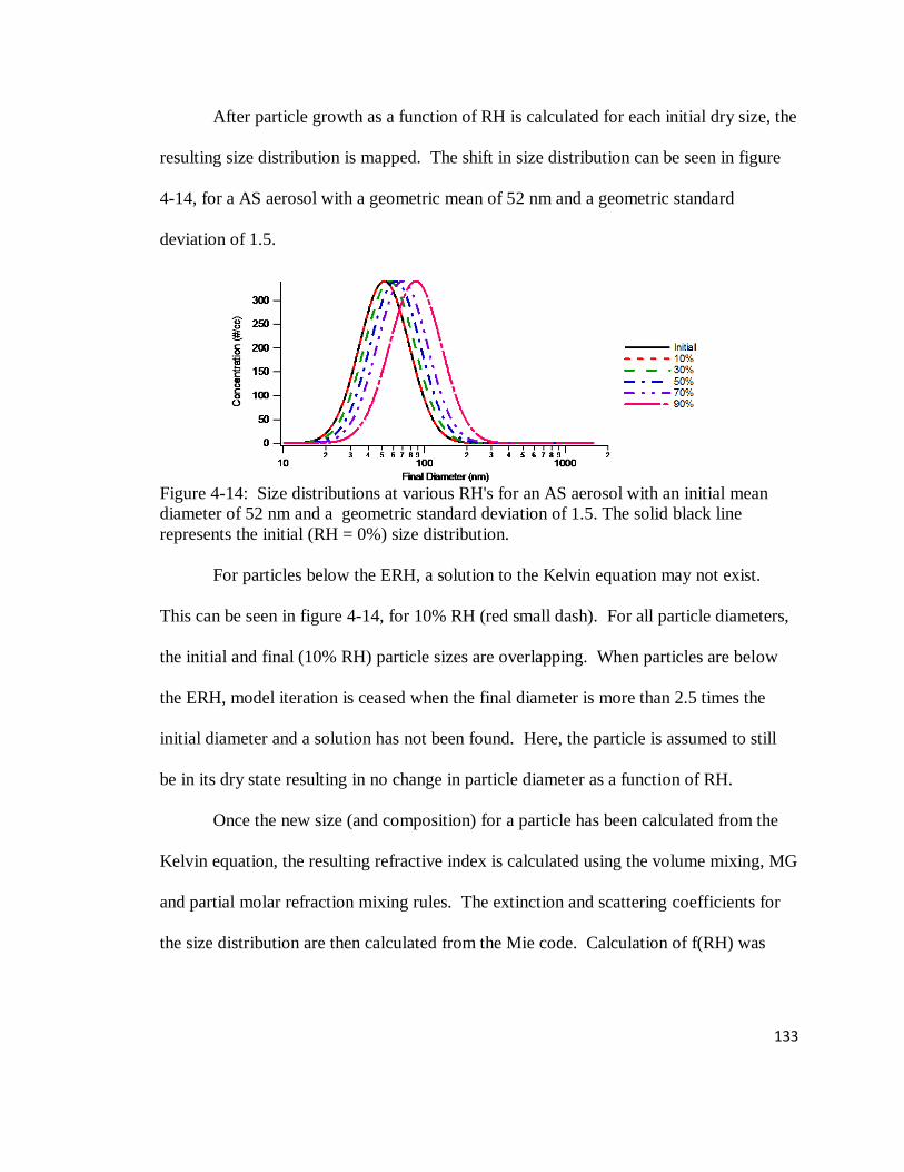
133
After particle growth as a function of RH is calculated for each initial dry size, the
resulting size distribution is mapped. The shift in size distribution can be seen in figure
4-14, for a AS aerosol with a geometric mean of 52 nm and a geometric standard
deviation of 1.5.
Figure 4-14: Size distributions at various RH's for an AS aerosol with an initial mean
diameter of 52 nm and a geometric standard deviation of 1.5. The solid black line
represents the initial (RH = 0%) size distribution.
For particles below the ERH, a solution to the Kelvin equation may not exist.
This can be seen in figure 4-14, for 10% RH (red small dash). For all particle diameters,
the initial and final (10% RH) particle sizes are overlapping. When particles are below
the ERH, model iteration is ceased when the final diameter is more than 2.5 times the
initial diameter and a solution has not been found. Here, the particle is assumed to still
be in its dry state resulting in no change in particle diameter as a function of RH.
Once the new size (and composition) for a particle has been calculated from the
Kelvin equation, the resulting refractive index is calculated using the volume mixing, MG
and partial molar refraction mixing rules. The extinction and scattering coefficients for
the size distribution are then calculated from the Mie code. Calculation of f(RH) was
134
done assuming the dry RH was 10%, the average RH of the Dry channel of the HC-
CRDT.
4.8. AS Results
A 100 ppm AS solution was aerosolized for measurement by the HC-CRDT. RH
and temperature data for each channel are shown versus time in fractional day of year
(DOY) in figures 4-15 and 4-16, respectively. On all plots, the Ambient-A, Ambient-B,
Dry and Humidified channels are represented as black circles, red squares, green triangles
and blue stars, respectively. Shading on the Dry and Humidified channels represents
different locations (upstream/downstream from the instrument) of RH/T sensors on the
same channel.
The RH of the dilution air for the 100 ppm AS aerosol was started high and
slowly decreased over time, as the ambient RH measured on the Ambient-A, Ambient-B
and at the valve on the Dry channel show(Fig. 4-13). The RH of the Humidified channel
was constant at 71.7 ± 0.6% RH immediately after the humidifier and 80.7 ± 0.5% RH at
the cavity exit. The Dry channel RH was also constant at 4.2 ± 0.2% RH immediately
after the dryer and 7.7 ± 0.3% at cavity exit. The Vaisala HMP50 RH/T sensors used in
this study have stated accuracies of ± 3% RH and ± 0.6°C. The RH stability of these
sensors is quoted as ± 2% over 2 years. Thus, these measurement differences are within
the limits of measurement accuracy for these sensors. For comparison to modeled
results, the RH and temperature of the aerosol stream at the cavity exit was taken since
this is closest to the CRD measurement within the instrument.

135
Figure 4-15: Plot of 4 minute averaged 100 ppm AS RH data versus fractional day of
year (DOY) measured by the Ambient-A (black circles), Ambient-B (red squares), Dry
(green triangles) and Humidified (blue stars) channels. Different color shades represent
multiple RH measurements on the same channel.
Figure 4-16: Plot of 4 minute averaged 100 ppm AS temperature data versus time in
fractional day of year (DOY) measured by the Ambient-A (black circles), Ambient-B
(red squares), Dry (green triangles) and Humidified (blue stars) channels. Different color
shades represent multiple RH measurements on the same channel. The Dry channel's
upstream temperature is omitted due to sensor malfunction.
Extinction coefficients of the 100 ppm AS aerosol measured at the visible
wavelength by all channels of the HC-CRDT are shown in figure 4-17. All data points
represent 4 minute averages. As the RH of the dilution air is decreased, the measured
extinction coefficients on all channels decrease; an small increase in the RH was noticed
before the RH started decreasing in the middle of the data set. Measured extinction
values on the ambient channels tracked with this trend.
100
80
60
40
20
0
RH
(%
)
286.00285.98285.96285.94285.92285.90
DOY
Ambient-A Ambient-B Dry Valve Dry Post-HC Dry Post-Cavity Humidified Post-HC Humidified Post-Cavity
24
22
20
18
16
Te
mp
era
ture
(°C
)
286.00285.98285.96285.94285.92285.90
DOY
Ambient-A Ambient-B Dry Post-HC Dry Post-Cavity Humidified Post-HC Humidified Post-Cavity
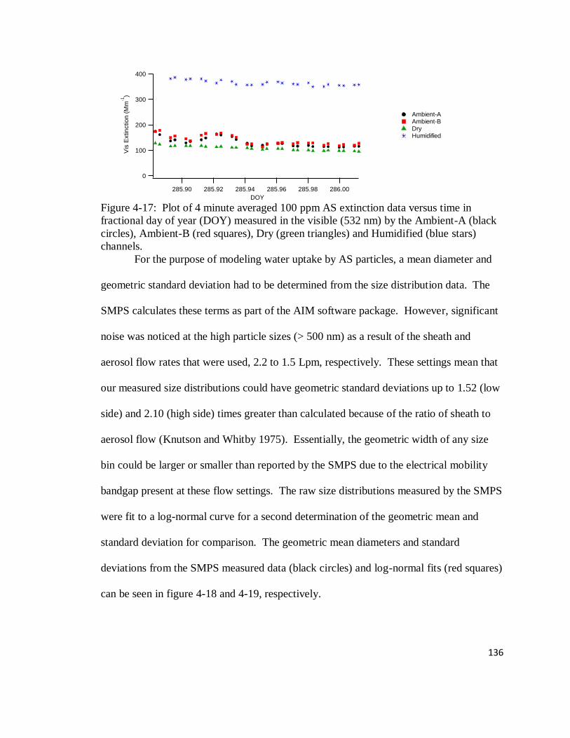
136
Figure 4-17: Plot of 4 minute averaged 100 ppm AS extinction data versus time in
fractional day of year (DOY) measured in the visible (532 nm) by the Ambient-A (black
circles), Ambient-B (red squares), Dry (green triangles) and Humidified (blue stars)
channels.
For the purpose of modeling water uptake by AS particles, a mean diameter and
geometric standard deviation had to be determined from the size distribution data. The
SMPS calculates these terms as part of the AIM software package. However, significant
noise was noticed at the high particle sizes (> 500 nm) as a result of the sheath and
aerosol flow rates that were used, 2.2 to 1.5 Lpm, respectively. These settings mean that
our measured size distributions could have geometric standard deviations up to 1.52 (low
side) and 2.10 (high side) times greater than calculated because of the ratio of sheath to
aerosol flow (Knutson and Whitby 1975). Essentially, the geometric width of any size
bin could be larger or smaller than reported by the SMPS due to the electrical mobility
bandgap present at these flow settings. The raw size distributions measured by the SMPS
were fit to a log-normal curve for a second determination of the geometric mean and
standard deviation for comparison. The geometric mean diameters and standard
deviations from the SMPS measured data (black circles) and log-normal fits (red squares)
can be seen in figure 4-18 and 4-19, respectively.
400
300
200
100
0
Vis
Extin
ctio
n (
Mm
-1)
286.00285.98285.96285.94285.92285.90
DOY
Ambient-A Ambient-B Dry Humidified
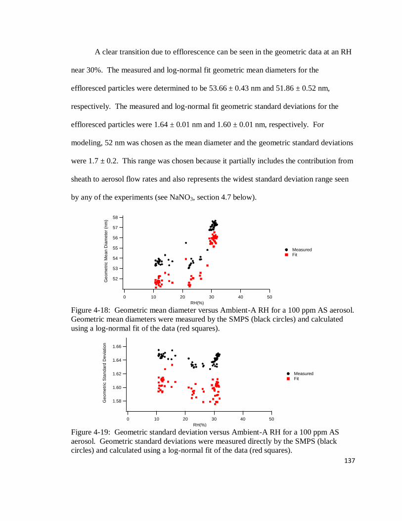
137
A clear transition due to efflorescence can be seen in the geometric data at an RH
near 30%. The measured and log-normal fit geometric mean diameters for the
effloresced particles were determined to be 53.66 ± 0.43 nm and 51.86 ± 0.52 nm,
respectively. The measured and log-normal fit geometric standard deviations for the
effloresced particles were 1.64 ± 0.01 nm and 1.60 ± 0.01 nm, respectively. For
modeling, 52 nm was chosen as the mean diameter and the geometric standard deviations
were 1.7 ± 0.2. This range was chosen because it partially includes the contribution from
sheath to aerosol flow rates and also represents the widest standard deviation range seen
by any of the experiments (see NaNO3, section 4.7 below).
Figure 4-18: Geometric mean diameter versus Ambient-A RH for a 100 ppm AS aerosol.
Geometric mean diameters were measured by the SMPS (black circles) and calculated
using a log-normal fit of the data (red squares).
Figure 4-19: Geometric standard deviation versus Ambient-A RH for a 100 ppm AS
aerosol. Geometric standard deviations were measured directly by the SMPS (black
circles) and calculated using a log-normal fit of the data (red squares).
58
57
56
55
54
53
52
Ge
om
etr
ic M
ea
n D
iam
ete
r (n
m)
50403020100
RH(%)
Measured Fit
1.66
1.64
1.62
1.60
1.58Ge
om
etr
ic S
tan
da
rd D
evia
tio
n
50403020100
RH(%)
Measured Fit
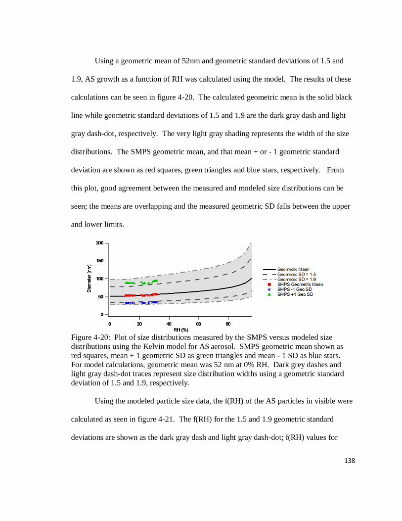
138
Using a geometric mean of 52nm and geometric standard deviations of 1.5 and
1.9, AS growth as a function of RH was calculated using the model. The results of these
calculations can be seen in figure 4-20. The calculated geometric mean is the solid black
line while geometric standard deviations of 1.5 and 1.9 are the dark gray dash and light
gray dash-dot, respectively. The very light gray shading represents the width of the size
distributions. The SMPS geometric mean, and that mean + or - 1 geometric standard
deviation are shown as red squares, green triangles and blue stars, respectively. From
this plot, good agreement between the measured and modeled size distributions can be
seen; the means are overlapping and the measured geometric SD falls between the upper
and lower limits.
Figure 4-20: Plot of size distributions measured by the SMPS versus modeled size
distributions using the Kelvin model for AS aerosol. SMPS geometric mean shown as
red squares, mean + 1 geometric SD as green triangles and mean - 1 SD as blue stars.
For model calculations, geometric mean was 52 nm at 0% RH. Dark grey dashes and
light gray dash-dot traces represent size distribution widths using a geometric standard
deviation of 1.5 and 1.9, respectively.
Using the modeled particle size data, the f(RH) of the AS particles in visible were
calculated as seen in figure 4-21. The f(RH) for the 1.5 and 1.9 geometric standard
deviations are shown as the dark gray dash and light gray dash-dot; f(RH) values for

139
modeled data was calculated assuming a dry RH of 10%. The f(RH) for the Ambient-A
relative to the Dry and the Humidified relative to the dry are shown as the black circles
and blue stars, respectively. Good agreement between the Ambient-A and Humidified
data relative to the modeled data can be seen as both data sets fall on or between the
standard deviation bounds of 1.5 and 1.9.
Figure 4-21: Plot of f(RH) in the visible for the AS size distributions modeled in figure
4-20 using partial molar refraction. Geometric mean diameter was taken to be 52 nm.
Dashed dark gray line and dash-dot light gray line represent geometric standard
deviations of 1.5 and 1.9 respectively. Lighter shading in between these 2 traces show
the range of f(RH) values calculated between these 2 limits. Solid black dot and blue
stars are the Ambient-A and Humidified channel visible f(RH) values calculated relative
to the dry channel, respectively.
Calculated γ(RH) values for the visible are shown in figure 4-22. A natural log-
linear fit of all 3 data points was done between the Ambient-A, Humidified and Dry
channels in addition to calculation of discrete values using equation 4-6 between the
Humidified and Ambient-A channels (red squares), Humidified and Dry channels (blue
stars) and Ambient-A and Dry channels (green triangles). The gray box through the
middle of the data is the range of modeled γ(RH) calculated from figure 4-21. The γ(RH)
value between the fit and both data sets using the humidified channel show good
agreement with each other and the model. This results From AS having a smooth growth

140
curve with RH; AS does effloresce and deliquesce, however the magnitude of growth
increase (c in equation 4-4) is small. For salts showing stronger efflorescence and
deliquescence, such as sodium chloride, a difference between these 3 values is indicative
of this efflorescence/deliquescence occurring. The Ambient-A to Dry γ(RH) shows a
large amount of scatter and does not agree well with the other values. This is a result of
small differences between the measured extinctions and RH values. For this reason, the
γ(RH) values are the most reliable when the RH of the ambient channel is situated
between the Humidified and Dry channels.
Figure 4-22: Calculated γ(RH) in the visible using a natural log linear fit (black circles)
for the Humidified relative to Ambient-A channel (red squares), Humidified relative to
dry channel (blue stars), Ambient-A relative to dry channel (green triangles). The range
of modeled γ(RH) values are shown as the gray box.
The 4 minute averaged AS data for the UV can be seen in figure 4-23. As with
the visible data set, changes in extinction track well with changes in the RH.
Comparisons of the measured f(RH) values to the modeled ones can be seen in figure 4-
24; the refractive index of AS in the UV was taken to be 1.55 from a polynomial fit of the
data in (Toon, Pollack et al. 1976). The f(RH) for the Ambient-A channel agrees well
with the model. However, the f(RH) on the Humidified channel does not agree as well
and stems directly from the raw ring-downs. Base extinction on the Humidified channel
4
3
2
1
0
Ga
mm
a(V
is)
286.00285.98285.96285.94285.92285.90
DOY
3-pt fit Humidified -> Ambient-A Humidified -> Dry Ambient-A -> Dry

141
was approximately 4100 Mm-1
so the accuracy of the measured values is questionable. In
reality, the measured aerosol extinction should have been near 1000 Mm-1
however
separating out this much extinction from noise at the already short ring-down times is
near impossible.
Figure 4-23: Plot of 4 minute averaged 100 ppm AS data measured in the UV (355 nm)
by the Ambient-A (black circles), Ambient-B (red squares), Dry (green triangles) and
Humidified (blue stars) channels.
Figure 4-24: Plot of f(RH) in the UV for the AS size distributions modeled in figure 4-20
using partial molar refraction. Geometric mean diameter was taken to be 52 nm. Dashed
dark gray line and dash-dot light gray line represent geometric standard deviations of 1.5
and 1.9 respectively. Lighter shading in between these 2 traces show the range of f(RH)
values calculated between these 2 limits. Solid black dot and blue stars are the Ambient-
A and Humidified channel visible f(RH) values calculated relative to the dry channel,
respectively.
The 4 minute averaged AS data for the IR can be seen in figure 4-25. Again,
extinction tracks well with RH. Comparisons of the measured f(RH) values to the
modeled ones can be seen in figure 4-26; the refractive index of AS in the IR was taken
600
550
500
450
400
350
300
UV
Extin
ctio
n (
Mm
-1)
286.00285.98285.96285.94285.92285.90
DOY
Ambient-A Ambient-B Dry Humidified

142
to be 1.51 from a polynomial fit of the data in (Toon, Pollack et al. 1976). All measured
and model values agree well.
Figure 4-25: Plot of 4 minute averaged 100 ppm AS data measured in the IR (1064 nm)
by the Ambient-A (black circles), Ambient-B (red squares), Dry (green triangles) and
Humidified (blue stars) channels.
Figure 4-26: Plot of f(RH) in the IR for the AS size distributions modeled in figure 4-22
using partial molar refraction. Geometric mean diameter was taken to be 52 nm. Dashed
dark gray line and dash-dot light gray line represent geometric standard deviations of 1.5
and 1.9 respectively. Lighter shading in between these 2 traces show the range of f(RH)
values calculated between these 2 limits. Solid black dot and blue stars are the Ambient-
A and Humidified channel visible f(RH) values calculated relative to the dry channel,
respectively.
4.9. NaNO3 Results
Sodium nitrate is an interesting particle because of its behavior upon hydration
and dehydration. Crystalline NaNO3 does effloresce and deliquesce like most other ionic
salts; aerosols produced directly from the crystalline solid will show this trend. However,
if NaNO3 is aerosolized from a liquid solution, the efflorescence and deliquescence
100
80
60
40
20
0
IR E
xtin
ctio
n (
Mm
-1)
286.00285.98285.96285.94285.92285.90
DOY
Ambient-A Dry Humidified

143
effects are sometimes not seen; instead NaNO3 behaves more like a purely hygroscopic
aerosol presumably because it forms an amorphous solid (Gysel, Weingartner et al. 2001;
Hoffman, Laskin et al. 2004). This lack of efflorescence can be seen in the normalized
size distributions versus Ambient-A RH shown in figure 4-27. Some of size distributions
that were collected are not shown for clarity. In this figure it is evident that as RH
decreases, the size distribution smoothly shifts to smaller particle sizes. If prompt
efflorescence/deliquescence were being observed, then a sharp transition would have
been evident.
Figure 4-27: Normalized size distributions of NaNO3 as a function of RH. (Some of the
size distributions collected have been removed for clarity.
A 100 ppm NaNO3 solution was aerosolized for measurement by the HC-CRDT.
RH and temperature data for each channel are shown in figures 4-28 and 4-29,
respectively. On all plots, the Ambient-A, Ambient-B, Dry and Humidified channels are
represented as black circles, red squares, green triangles and blue stars, respectively.
Shading on the Dry and Humidified channels represents different locations
(upstream/downstream from the instrument) of RH/T sensors on the same channel.
1.0
0.8
0.6
0.4
0.2
0.02 3 4 5 6 7 8 9
1002 3 4 5 6 7 8 9
Diameter (nm)
35
30
25
20
15
Am
bie
nt-A
RH
(%)
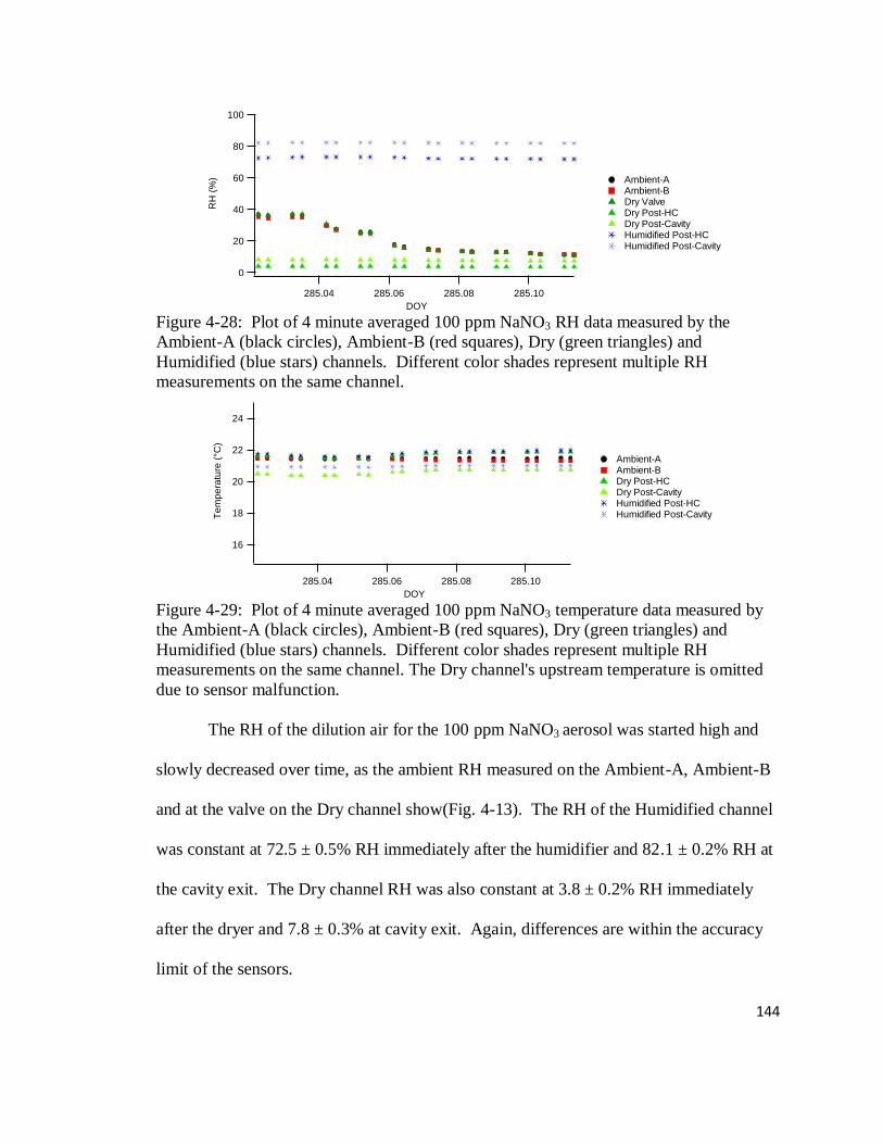
144
Figure 4-28: Plot of 4 minute averaged 100 ppm NaNO3 RH data measured by the
Ambient-A (black circles), Ambient-B (red squares), Dry (green triangles) and
Humidified (blue stars) channels. Different color shades represent multiple RH
measurements on the same channel.
Figure 4-29: Plot of 4 minute averaged 100 ppm NaNO3 temperature data measured by
the Ambient-A (black circles), Ambient-B (red squares), Dry (green triangles) and
Humidified (blue stars) channels. Different color shades represent multiple RH
measurements on the same channel. The Dry channel's upstream temperature is omitted
due to sensor malfunction.
The RH of the dilution air for the 100 ppm NaNO3 aerosol was started high and
slowly decreased over time, as the ambient RH measured on the Ambient-A, Ambient-B
and at the valve on the Dry channel show(Fig. 4-13). The RH of the Humidified channel
was constant at 72.5 ± 0.5% RH immediately after the humidifier and 82.1 ± 0.2% RH at
the cavity exit. The Dry channel RH was also constant at 3.8 ± 0.2% RH immediately
after the dryer and 7.8 ± 0.3% at cavity exit. Again, differences are within the accuracy
limit of the sensors.
100
80
60
40
20
0
RH
(%
)
285.10285.08285.06285.04
DOY
Ambient-A Ambient-B Dry Valve Dry Post-HC Dry Post-Cavity Humidified Post-HC Humidified Post-Cavity
24
22
20
18
16
Te
mp
era
ture
(°C
)
285.10285.08285.06285.04
DOY
Ambient-A Ambient-B Dry Post-HC Dry Post-Cavity Humidified Post-HC Humidified Post-Cavity
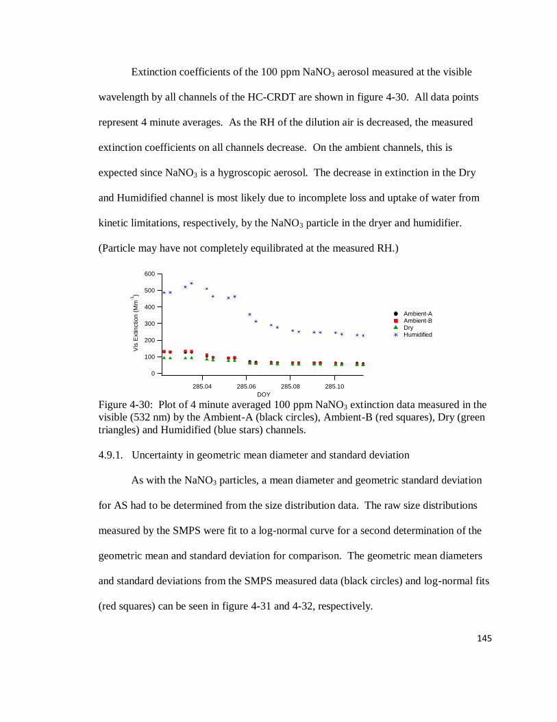
145
Extinction coefficients of the 100 ppm NaNO3 aerosol measured at the visible
wavelength by all channels of the HC-CRDT are shown in figure 4-30. All data points
represent 4 minute averages. As the RH of the dilution air is decreased, the measured
extinction coefficients on all channels decrease. On the ambient channels, this is
expected since NaNO3 is a hygroscopic aerosol. The decrease in extinction in the Dry
and Humidified channel is most likely due to incomplete loss and uptake of water from
kinetic limitations, respectively, by the NaNO3 particle in the dryer and humidifier.
(Particle may have not completely equilibrated at the measured RH.)
Figure 4-30: Plot of 4 minute averaged 100 ppm NaNO3 extinction data measured in the
visible (532 nm) by the Ambient-A (black circles), Ambient-B (red squares), Dry (green
triangles) and Humidified (blue stars) channels.
4.9.1. Uncertainty in geometric mean diameter and standard deviation
As with the NaNO3 particles, a mean diameter and geometric standard deviation
for AS had to be determined from the size distribution data. The raw size distributions
measured by the SMPS were fit to a log-normal curve for a second determination of the
geometric mean and standard deviation for comparison. The geometric mean diameters
and standard deviations from the SMPS measured data (black circles) and log-normal fits
(red squares) can be seen in figure 4-31 and 4-32, respectively.
600
500
400
300
200
100
0
Vis
Extin
ctio
n (
Mm
-1)
285.10285.08285.06285.04
DOY
Ambient-A Ambient-B Dry Humidified
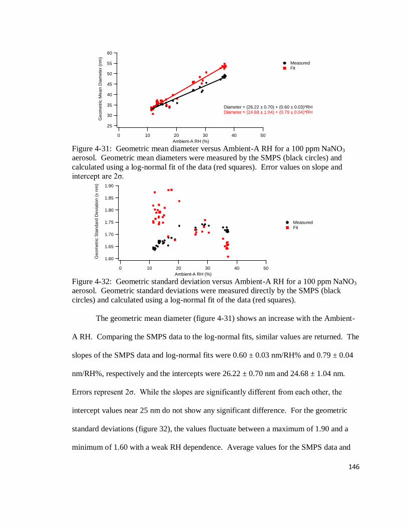
146
Figure 4-31: Geometric mean diameter versus Ambient-A RH for a 100 ppm NaNO3
aerosol. Geometric mean diameters were measured by the SMPS (black circles) and
calculated using a log-normal fit of the data (red squares). Error values on slope and
intercept are 2ζ.
Figure 4-32: Geometric standard deviation versus Ambient-A RH for a 100 ppm NaNO3
aerosol. Geometric standard deviations were measured directly by the SMPS (black
circles) and calculated using a log-normal fit of the data (red squares).
The geometric mean diameter (figure 4-31) shows an increase with the Ambient-
A RH. Comparing the SMPS data to the log-normal fits, similar values are returned. The
slopes of the SMPS data and log-normal fits were 0.60 ± 0.03 nm/RH% and 0.79 ± 0.04
nm/RH%, respectively and the intercepts were 26.22 ± 0.70 nm and 24.68 ± 1.04 nm.
Errors represent 2ζ. While the slopes are significantly different from each other, the
intercept values near 25 nm do not show any significant difference. For the geometric
standard deviations (figure 32), the values fluctuate between a maximum of 1.90 and a
minimum of 1.60 with a weak RH dependence. Average values for the SMPS data and
60
55
50
45
40
35
30
25
Ge
om
etr
ic M
ea
n D
iam
ete
r (n
m)
50403020100
Ambient-A RH (%)
Measured Fit
Diameter = (26.22 ± 0.70) + (0.60 ± 0.03)*RHDiameter = (24.68 ± 1.04) + (0.79 ± 0.04)*RH
1.90
1.85
1.80
1.75
1.70
1.65
1.60Ge
om
etr
ic S
tan
da
rd D
evia
tio
n (
± n
m)
50403020100
Ambient-A RH (%)
Measured Fit
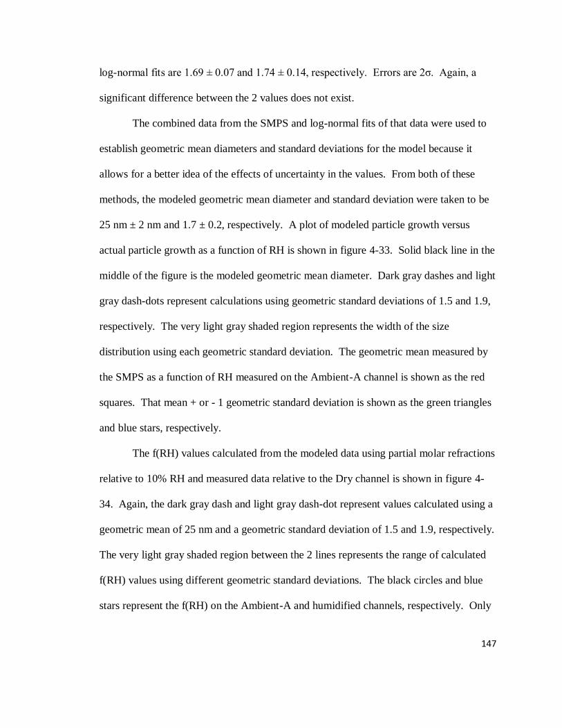
147
log-normal fits are 1.69 ± 0.07 and 1.74 ± 0.14, respectively. Errors are 2ζ. Again, a
significant difference between the 2 values does not exist.
The combined data from the SMPS and log-normal fits of that data were used to
establish geometric mean diameters and standard deviations for the model because it
allows for a better idea of the effects of uncertainty in the values. From both of these
methods, the modeled geometric mean diameter and standard deviation were taken to be
25 nm ± 2 nm and 1.7 ± 0.2, respectively. A plot of modeled particle growth versus
actual particle growth as a function of RH is shown in figure 4-33. Solid black line in the
middle of the figure is the modeled geometric mean diameter. Dark gray dashes and light
gray dash-dots represent calculations using geometric standard deviations of 1.5 and 1.9,
respectively. The very light gray shaded region represents the width of the size
distribution using each geometric standard deviation. The geometric mean measured by
the SMPS as a function of RH measured on the Ambient-A channel is shown as the red
squares. That mean + or - 1 geometric standard deviation is shown as the green triangles
and blue stars, respectively.
The f(RH) values calculated from the modeled data using partial molar refractions
relative to 10% RH and measured data relative to the Dry channel is shown in figure 4-
34. Again, the dark gray dash and light gray dash-dot represent values calculated using a
geometric mean of 25 nm and a geometric standard deviation of 1.5 and 1.9, respectively.
The very light gray shaded region between the 2 lines represents the range of calculated
f(RH) values using different geometric standard deviations. The black circles and blue
stars represent the f(RH) on the Ambient-A and humidified channels, respectively. Only

148
the average geometric mean diameter of 25 nm is shown as small shifts in mean diameter
do not significantly affect model results.
Figure 4-33: Plot of size distributions measured by the SMPS versus modeled size
distributions using the Kelvin model for NaNO3 aerosol. SMPS geometric mean shown
as red squares, mean + 1 geometric SD as green triangles and mean - 1 SD as blue stars.
For model calculations, geometric mean was 25 nm at 0% RH. Dark grey dashes and
light gray dash-dot traces represent size distribution widths using a geometric standard
deviation of 1.5 and 1.9, respectively.
Figure 4-34: Plot of f(RH) in the visible for the size distributions modeled in figure 4-22
using partial molar refraction. Geometric mean diameter was taken to be 25 nm. Dashed
dark gray line and dash-dot light gray line represent geometric standard deviations of 1.5
and 1.9 respectively. Lighter shading in between these 2 traces show the range of f(RH)
values calculated between these 2 limits. Solid black dot and blue stars are the Ambient-
A and Humidified channel visible f(RH) values calculated relative to the dry channel,
respectively.
From figure 4-33, it is evident that the size distributions measured by the SMPS
and those calculated using the model do not agree well; the model significantly under-
predicts changes in particle diameter as a function of RH. However, from the measured
149
and calculated f(RH) values in figure 4-34, it appears that the calculations are modeling
the optical properties of the system reasonably accurately using the parameter set given.
The disagreement may stem from a kinetically limited loss and gain of water by
amorphous NaNO3; NaNO3 particles have been previously shown to adopt a metastable
amorphous state upon drying to very low RH and under vacuum conditions (Hoffman,
Laskin et al. 2004). Kinetically limited deliquescence and efflorescence in similar semi-
solid amorphous substances on time scales less than minutes to hours has been linked to
high viscosity and low diffusivity of water into or out of the particle (Mikhailov,
Vlasenko et al. 2009).
The aerosols measured by the SMPS were sampled immediately after being
drawn into the second mixing chamber (through an impactor). The RH of these aerosols
was measured in the Ambient-A channel at approximately the same time, but on a
separate flow line. The extinction coefficient measurements in all channels of the HC-
CRDT occurred significantly after the size distributions were measured by the SMPS
(approximately 20 sec). Particles must travel through roughly 3m of flow lines after the
second mixing chamber before reaching the CRD (the valving system, RH control system
and NephCams are all upstream of the ring-down measurement). The particle sizes
measured by the SMPS may represent an over-estimate of the particles measured in the
CRD if the aerosol has not fully equilibrated at the desired RH. Further, the extra
equilibration time allowed by the CRD measurement may not even be long enough to get
NaNO3 into its dry state.
This kinetically limited loss and uptake of water by NaNO3 can also be seen in the
raw ring-down data shown in figure 4-30. As the RH is decreased in time (figure 4-28)

150
the extinction measured by all of the channels decreases. In the Dry channel, the RH
after the ring-down measurement remained constant at around 8% RH. As the RH of the
incoming aerosol was decreased, the extent of equilibration of the Dry channel was
effectively increased because of a decrease in the humidity gradient (ΔRH) between the
ambient and Dry channels. As a result, the extinction coefficients measured in the Dry
channel decreased. The reverse is true on the Humidified channel which maintained a
constant RH near 82% after the ring-down measurement. As the RH of the incoming
aerosol decreased, the extinction coefficient measurements in the Humidified channel
also decreased due to an effective decrease in equilibration time for growth. The result is
a wider range of calculated f(RH) values than would be expected when the RH was stable
in time. This effect can also skew the geometric standard deviation of the particles being
measured. Larger particles will be less affected by the kinetically limited uptake of water
due to the Kelvin effect, and as a result, the width of the size distributions can be larger
than those modeled here.
This kinetic effect is not expected to be as pronounced for the other aerosols. The
geometric mean diameters of all other particle types are approximately twice as large as
NaNO3; 60 nm versus 25 nm, so the NaNO3 particles have to lose approximately 8 times
as much water after generation in the same amount of time. Further, other salts exhibit
prompt efflorescence; a rapid transition from an aqueous solution to a solid salt particle
with some amount of water adsorbed to the surface. The surface water then quickly
dissipates. With the NaNO3 particles, the particle is a solution that is becoming more and
more concentrated with decreasing RH as it transitions to an amorphous solid (Hoffman,
Laskin et al. 2004). The lack of an clear phase transition implies that loss of water is

151
kinetically limited by how quickly it can be removed from the concentrated solution
rather than how quickly pure water can evaporate from a highly curved solid surface.
A final point about the size distributions that should be recognized. The SMPS
recirculates excess flow as sheath air and there is a finite RH equilibration time for this
process. When the incoming aerosol RH is changing, the RH measured by the HC-
CRDT on the ambient channel is not necessarily the same as the RH inside of the DMA.
For experiments where the RH was decreased from an initially high value, the RH inside
of the DMA could be higher than that recorded in the HC-CRDT. As a result, particles
may be presumed to be larger at the measured RH than they actually are. The reverse is
also true when doing experiments where the RH is increased from an initially low value.
Effects where the RH inside of the SMPS is different than that in the rest of the system
because of the sheath flow have been documented (Hämeri, Laaksonen et al. 2001;
Biskos, Malinowski et al. 2006; Biskos, Paulsen et al. 2006; Biskos, Russell et al. 2006).
Because of the slow growth/shrinkage of NaNO3 as function of RH, this effect is
expected to be minimal for the current aerosol but may be an issue for other particle
types.
Measured 4 minute averages of the NaNO3 aerosol in the UV and IR can be seen
in figures 4-35 and 4-37, respectively. The modeled and measured f(RH) values for the
UV and IR can be seen in figures 4-36 and 4-38, respectively. The refractive index of
NaNO3 in the UV and IR was assumed to be 1.61 and 1.57, respectively. A literature
value for these 2 wavelengths was not available so the trend that refractive index changed
by 0.02 between wavelengths (as is the case for AS and NaCl) was applied. In the UV,
good agreement between the Ambient-A channel and f(RH) exists, but the Humidified
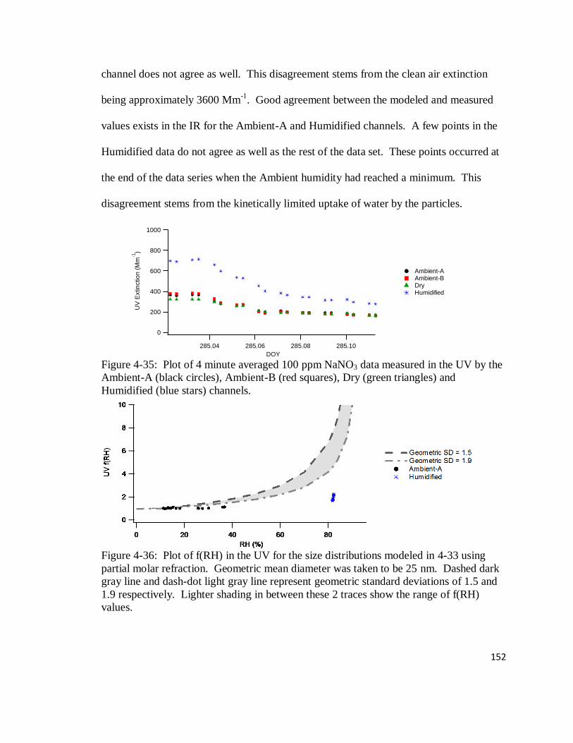
152
channel does not agree as well. This disagreement stems from the clean air extinction
being approximately 3600 Mm-1
. Good agreement between the modeled and measured
values exists in the IR for the Ambient-A and Humidified channels. A few points in the
Humidified data do not agree as well as the rest of the data set. These points occurred at
the end of the data series when the Ambient humidity had reached a minimum. This
disagreement stems from the kinetically limited uptake of water by the particles.
Figure 4-35: Plot of 4 minute averaged 100 ppm NaNO3 data measured in the UV by the
Ambient-A (black circles), Ambient-B (red squares), Dry (green triangles) and
Humidified (blue stars) channels.
Figure 4-36: Plot of f(RH) in the UV for the size distributions modeled in 4-33 using
partial molar refraction. Geometric mean diameter was taken to be 25 nm. Dashed dark
gray line and dash-dot light gray line represent geometric standard deviations of 1.5 and
1.9 respectively. Lighter shading in between these 2 traces show the range of f(RH)
values.
1000
800
600
400
200
0
UV
Extin
ctio
n (
Mm
-1)
285.10285.08285.06285.04
DOY
Ambient-A Ambient-B Dry Humidified

153
Figure 4-37: Plot of 4 minute averaged 100 ppm NaNO3 data measured in the IR by the
Ambient-A (black circles), Ambient-B (red squares), Dry (green triangles) and
Humidified (blue stars) channels.
Figure 4-38: Plot of f(RH) in the IR for the size distributions modeled in figure 4-33
using partial molar refraction. Geometric mean diameter was taken to be 25 nm. Dashed
dark gray line and dash-dot light gray line represent geometric standard deviations of 1.5
and 1.9 respectively. Lighter shading in between these 2 traces show the range of f(RH)
values.
4.10. NaCl Results
A 20 ppm NaCl aerosol was measured using the HC-CRDT and modeled using
the Kelvin model described above. Unlike the NaNO3 aerosol, NaCl is a strongly
hygroscopic aerosol that exhibits distinct and significant efflorescence and deliquescence.
The RH and temperature temporal profiles for a NaCl aerosol experiment is shown in
figures 4-39 and 4-40.
100
80
60
40
20
0
IR E
xtin
ctio
n (
Mm
-1)
285.10285.08285.06285.04
DOY
Ambient-A Dry Humidified
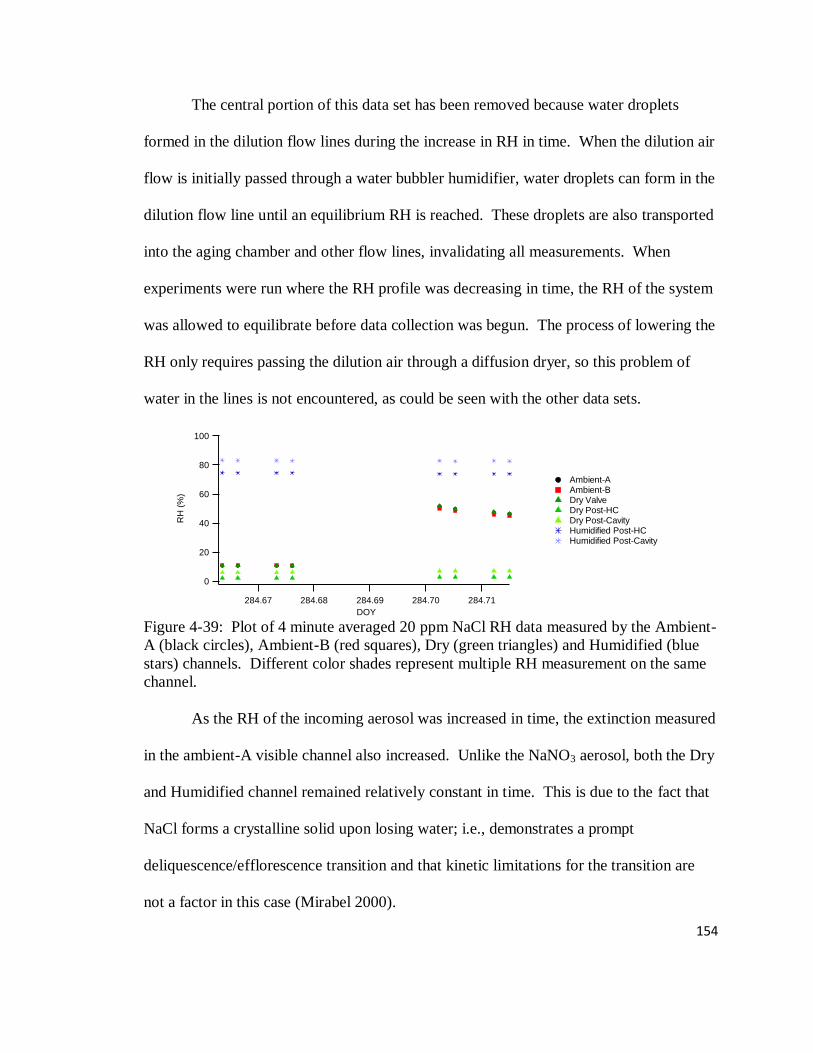
154
The central portion of this data set has been removed because water droplets
formed in the dilution flow lines during the increase in RH in time. When the dilution air
flow is initially passed through a water bubbler humidifier, water droplets can form in the
dilution flow line until an equilibrium RH is reached. These droplets are also transported
into the aging chamber and other flow lines, invalidating all measurements. When
experiments were run where the RH profile was decreasing in time, the RH of the system
was allowed to equilibrate before data collection was begun. The process of lowering the
RH only requires passing the dilution air through a diffusion dryer, so this problem of
water in the lines is not encountered, as could be seen with the other data sets.
Figure 4-39: Plot of 4 minute averaged 20 ppm NaCl RH data measured by the Ambient-
A (black circles), Ambient-B (red squares), Dry (green triangles) and Humidified (blue
stars) channels. Different color shades represent multiple RH measurement on the same
channel.
As the RH of the incoming aerosol was increased in time, the extinction measured
in the ambient-A visible channel also increased. Unlike the NaNO3 aerosol, both the Dry
and Humidified channel remained relatively constant in time. This is due to the fact that
NaCl forms a crystalline solid upon losing water; i.e., demonstrates a prompt
deliquescence/efflorescence transition and that kinetic limitations for the transition are
not a factor in this case (Mirabel 2000).
100
80
60
40
20
0
RH
(%
)
284.71284.70284.69284.68284.67
DOY
Ambient-A Ambient-B Dry Valve Dry Post-HC Dry Post-Cavity Humidified Post-HC Humidified Post-Cavity

155
Figure 4-40: Plot of 4 minute averaged 20 ppm NaCl temperature data measured by the
Ambient-A (black circles), Ambient-B (red squares), Dry (green triangles) and
Humidified (blue stars) channels. Different color shades represent multiple RH
measurements on the same channel. The Dry channel's valve temperature is omitted due
to sensor malfunction.
Figure 4-41: Plot of 4 minute averaged 20 ppm NaCl extinction data measured in the
visible by the Ambient-A (black circles), Ambient-B (red squares), Dry (green triangles)
and Humidified (blue stars) channels.
The RH in the ambient channel can clearly be seen to have increased in time
(figure 4-41). In figures 4-42, geometric mean diameters measured by the SMPS and
values calculated by a log-normal fit of the raw data (black circles and red squares,
respectively) are seen to have changed in response to the change in RH. At low RH, the
measured and fit average mean diameters are 43.11 ± 1.80 nm for the SMPS measured
and 46.80 ± 1.22 nm from the fits, respectively. As the ambient RH was increased these
values shifted to 55.18 ± 1.84 nm and 60.02 ± 1.91 nm. Toward the end of the
experiment, the geometric mean diameters appear to be decreasing a bit, which may be
24
22
20
18
16
Te
mp
era
ture
(°C
)
284.71284.70284.69284.68284.67
DOY
Ambient-A Ambient-B Dry Post-HC Dry Post-Cavity Humidified Post-HC Humidified Post-Cavity
400
300
200
100
0
Vis
Extin
ctio
n (
Mm
-1)
284.71284.70284.69284.68284.67
DOY
Ambient-A Ambient-B Dry Humidified
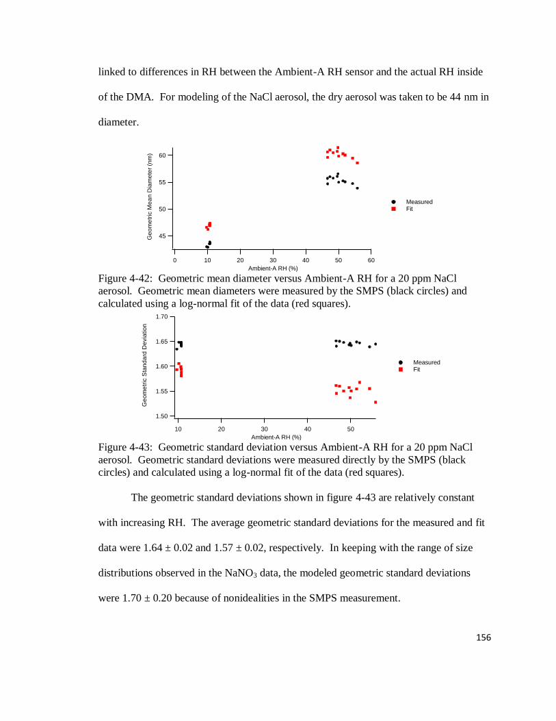
156
linked to differences in RH between the Ambient-A RH sensor and the actual RH inside
of the DMA. For modeling of the NaCl aerosol, the dry aerosol was taken to be 44 nm in
diameter.
Figure 4-42: Geometric mean diameter versus Ambient-A RH for a 20 ppm NaCl
aerosol. Geometric mean diameters were measured by the SMPS (black circles) and
calculated using a log-normal fit of the data (red squares).
Figure 4-43: Geometric standard deviation versus Ambient-A RH for a 20 ppm NaCl
aerosol. Geometric standard deviations were measured directly by the SMPS (black
circles) and calculated using a log-normal fit of the data (red squares).
The geometric standard deviations shown in figure 4-43 are relatively constant
with increasing RH. The average geometric standard deviations for the measured and fit
data were 1.64 ± 0.02 and 1.57 ± 0.02, respectively. In keeping with the range of size
distributions observed in the NaNO3 data, the modeled geometric standard deviations
were 1.70 ± 0.20 because of nonidealities in the SMPS measurement.
60
55
50
45Ge
om
etr
ic M
ea
n D
iam
ete
r (n
m)
6050403020100
Ambient-A RH (%)
Measured Fit
1.70
1.65
1.60
1.55
1.50
Ge
om
etr
ic S
tan
da
rd D
evia
tio
n
5040302010
Ambient-A RH (%)
Measured Fit
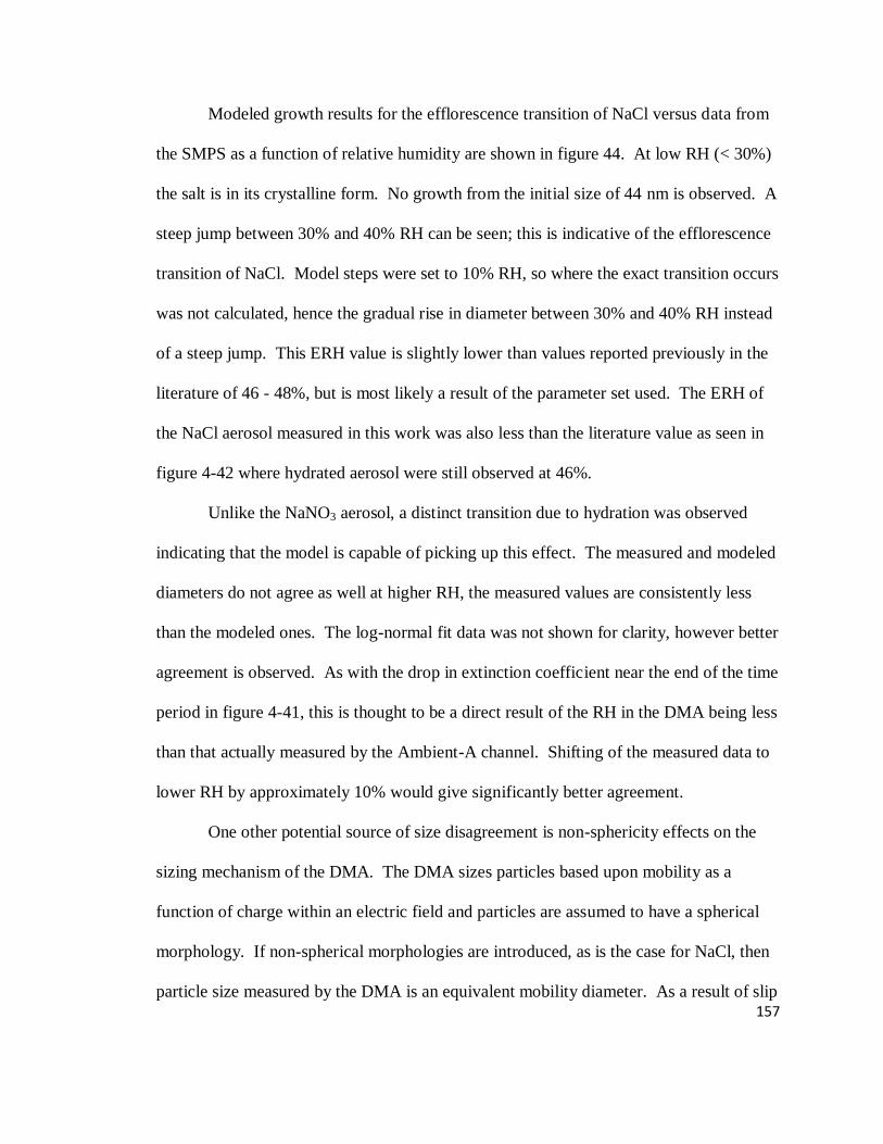
157
Modeled growth results for the efflorescence transition of NaCl versus data from
the SMPS as a function of relative humidity are shown in figure 44. At low RH (< 30%)
the salt is in its crystalline form. No growth from the initial size of 44 nm is observed. A
steep jump between 30% and 40% RH can be seen; this is indicative of the efflorescence
transition of NaCl. Model steps were set to 10% RH, so where the exact transition occurs
was not calculated, hence the gradual rise in diameter between 30% and 40% RH instead
of a steep jump. This ERH value is slightly lower than values reported previously in the
literature of 46 - 48%, but is most likely a result of the parameter set used. The ERH of
the NaCl aerosol measured in this work was also less than the literature value as seen in
figure 4-42 where hydrated aerosol were still observed at 46%.
Unlike the NaNO3 aerosol, a distinct transition due to hydration was observed
indicating that the model is capable of picking up this effect. The measured and modeled
diameters do not agree as well at higher RH, the measured values are consistently less
than the modeled ones. The log-normal fit data was not shown for clarity, however better
agreement is observed. As with the drop in extinction coefficient near the end of the time
period in figure 4-41, this is thought to be a direct result of the RH in the DMA being less
than that actually measured by the Ambient-A channel. Shifting of the measured data to
lower RH by approximately 10% would give significantly better agreement.
One other potential source of size disagreement is non-sphericity effects on the
sizing mechanism of the DMA. The DMA sizes particles based upon mobility as a
function of charge within an electric field and particles are assumed to have a spherical
morphology. If non-spherical morphologies are introduced, as is the case for NaCl, then
particle size measured by the DMA is an equivalent mobility diameter. As a result of slip
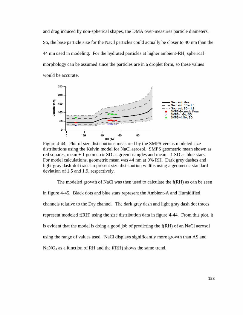
158
and drag induced by non-spherical shapes, the DMA over-measures particle diameters.
So, the base particle size for the NaCl particles could actually be closer to 40 nm than the
44 nm used in modeling. For the hydrated particles at higher ambient-RH, spherical
morphology can be assumed since the particles are in a droplet form, so these values
would be accurate.
Figure 4-44: Plot of size distributions measured by the SMPS versus modeled size
distributions using the Kelvin model for NaCl aerosol. SMPS geometric mean shown as
red squares, mean + 1 geometric SD as green triangles and mean - 1 SD as blue stars.
For model calculations, geometric mean was 44 nm at 0% RH. Dark grey dashes and
light gray dash-dot traces represent size distribution widths using a geometric standard
deviation of 1.5 and 1.9, respectively.
The modeled growth of NaCl was then used to calculate the f(RH) as can be seen
in figure 4-45. Black dots and blue stars represent the Ambient-A and Humidified
channels relative to the Dry channel. The dark gray dash and light gray dash dot traces
represent modeled f(RH) using the size distribution data in figure 4-44. From this plot, it
is evident that the model is doing a good job of predicting the f(RH) of an NaCl aerosol
using the range of values used. NaCl displays significantly more growth than AS and
NaNO3 as a function of RH and the f(RH) shows the same trend.

159
Figure 4-45: Plot of f(RH) in the visible for the size distributions modeled in figure 4-44
using partial molar refraction. Geometric mean diameter was taken to be 44 nm. Dashed
dark gray line and dash-dot light gray line represent geometric standard deviations of 1.5
and 1.9 respectively. Lighter shading in between these 2 traces show the range of f(RH)
values calculated between these 2 limits. Solid black dot and blue stars are the Ambient-
A and Humidified channel visible f(RH) values calculated relative to the Dry channel,
respectively.
The f(RH) model calculations versus actual f(RH) data in the IR and UV are
shown in figures 4-46 and 4-48, respectively. Figures 4-47 and 4-49 are the 4 minute
averaged extinction data for the IR and UV channels collected by the HC-CRDT,
respectively.
The f(RH) data in the IR shows good general agreement with model calculations
although there is slight disagreement for some of the data points. This disagreement is
most likely a result of the small absolute magnitude of the IR signals, many of the dry IR
measurements were at or near the LOQ for the HC-CRDT on that channel. As a result,
small fluctuations in measured values on the dry channel can cause significant fluctuation
in the calculated f(RH) data.

160
Figure 4-46: Plot of f(RH) in the IR for the size distributions modeled in figure 4-44
using partial molar refraction. Geometric mean diameter was taken to be 44 nm. Dashed
dark gray line and dash-dot light gray line represent geometric standard deviations of 1.5
and 1.9 respectively. Lighter shading in between these 2 traces show the range of f(RH)
values calculated between these 2 limits. Solid black dot and blue stars are the Ambient-
A and Humidified channel visible f(RH) values calculated relative to the Dry channel,
respectively.
Figure 4-47: Plot of 4 minute averaged 20 ppm NaCl data measured in the IR by the
Ambient-A (black circles), Dry (green triangles) and Humidified (blue stars) channels.
The f(RH) in the UV shows good agreement with model predictions, although
some of the measured f(RH) values are low relative to predictions especially the last 4
data points in figure 4-48. The clean air extinction during the NaCl data set started
around 3500 Mm-1
but ended around 3750 Mm-1
as a result of the water droplets in the
flow lines. This increase in the clean air extinction is most likely impacting the accuracy
of the measurement on the Humidified channel.
100
80
60
40
20
0
IR E
xtin
ctio
n (
Mm
-1)
284.71284.70284.69284.68284.67
DOY
Ambient-A Dry Humidified

161
Figure 4-48: Plot of f(RH) in the UV for the size distributions modeled in figure 4-44
using partial molar refraction. Geometric mean diameter was taken to be 44 nm. Dashed
dark gray line and dash-dot light gray line represent geometric standard deviations of 1.5
and 1.9 respectively. Lighter shading in between these 2 traces show the range of f(RH)
values calculated between these 2 limits. Solid black dot and blue stars are the Ambient-
A and Humidified channel visible f(RH) values calculated relative to the Dry channel,
respectively.
Figure 4-49: Plot of 4 minute averaged 20 ppm NaCl data measured in the UV by the
Ambient-A (black circles), Ambient-B (red squares), Dry (green triangles) and
Humidified (blue stars) channels.
4.10.1. NaCl γ(RH)
The NaCl aerosol provides a unique insight into the behavior of γ(RH) because of
the significant size loss upon efflorescing. Modeled values of γ(RH) in the IR, visible
and UV for an NaCl aerosol with a geometric mean of 44 nm and a geometric standard
deviation of 1.5 can be seen in table 4-10. High RH was taken to be 82%. NaCl
effloresces around 40%, so both the 10% and 30% RH particles are in their effloresced
state; the extinction values for each are identical. The 30% RH has a higher γ(RH)
700
600
500
400
300
200
100
0
UV
Extin
ctio
n (
Mm
-1)
284.71284.70284.69284.68284.67
DOY
Ambient-A Ambient-B Dry Humidified
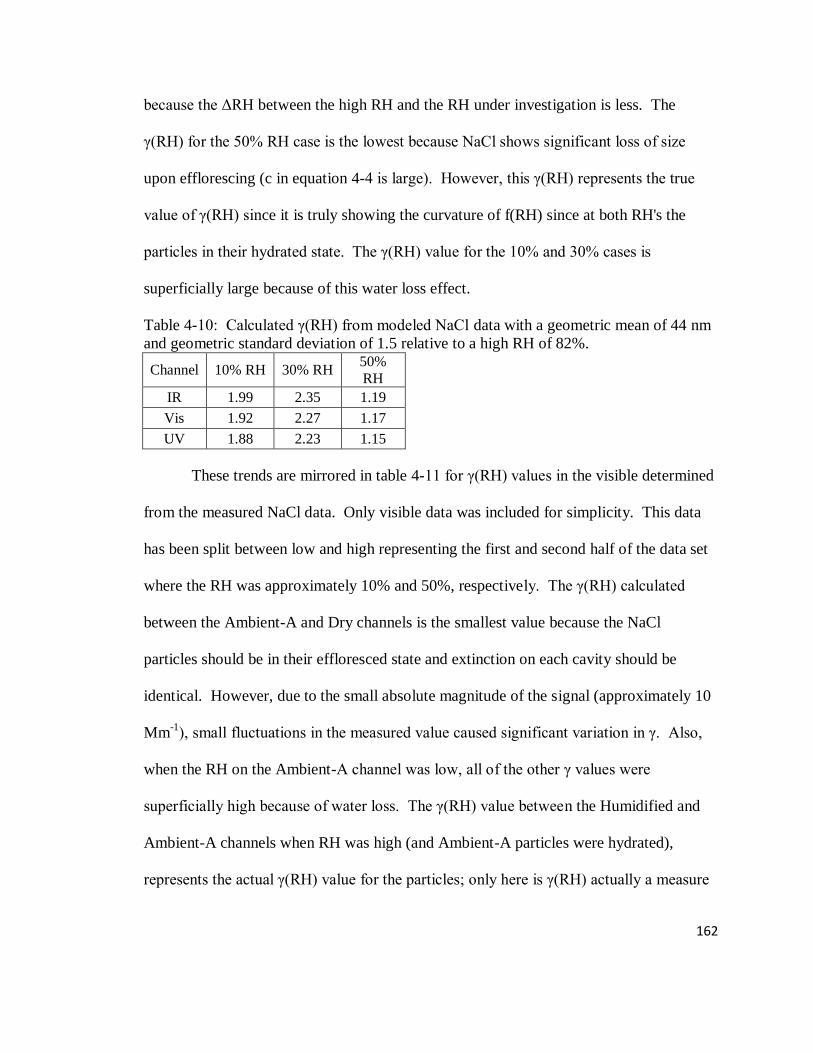
162
because the ΔRH between the high RH and the RH under investigation is less. The
γ(RH) for the 50% RH case is the lowest because NaCl shows significant loss of size
upon efflorescing (c in equation 4-4 is large). However, this γ(RH) represents the true
value of γ(RH) since it is truly showing the curvature of f(RH) since at both RH's the
particles in their hydrated state. The γ(RH) value for the 10% and 30% cases is
superficially large because of this water loss effect.
Table 4-10: Calculated γ(RH) from modeled NaCl data with a geometric mean of 44 nm
and geometric standard deviation of 1.5 relative to a high RH of 82%.
Channel 10% RH 30% RH 50%
RH
IR 1.99 2.35 1.19
Vis 1.92 2.27 1.17
UV 1.88 2.23 1.15
These trends are mirrored in table 4-11 for γ(RH) values in the visible determined
from the measured NaCl data. Only visible data was included for simplicity. This data
has been split between low and high representing the first and second half of the data set
where the RH was approximately 10% and 50%, respectively. The γ(RH) calculated
between the Ambient-A and Dry channels is the smallest value because the NaCl
particles should be in their effloresced state and extinction on each cavity should be
identical. However, due to the small absolute magnitude of the signal (approximately 10
Mm-1
), small fluctuations in the measured value caused significant variation in γ. Also,
when the RH on the Ambient-A channel was low, all of the other γ values were
superficially high because of water loss. The γ(RH) value between the Humidified and
Ambient-A channels when RH was high (and Ambient-A particles were hydrated),
represents the actual γ(RH) value for the particles; only here is γ(RH) actually a measure

163
of the curvature of f(RH). Because of this discrepancy between γ values, when calculated
discretely, between the Ambient-A, Humidified and Dry channels, it is possible to
determine whether efflorescent particles are present. Calculating a 3-point fit of the data
misses this effect entirely. In the event that all the values are the same, then efflorescence
is not present.
Table 4-11: Calculated γ(RH) in the visible from the measured NaCl data
RH 3-pt fit Humidified -> Ambient-A Humidified -> Dry Ambient-A -> Dry
Low 1.84 1.85 1.83 1.34
High 1.70 1.47 1.73 2.21
4.11. Nigrosin results
The f(RH) for a black carbon surrogate particle, Nigrosin, was also measured using the
HC-CRDT. Unlike black carbon, Nigrosin is water soluble and is not expected to form a
core-shell type morphology when exposed to elevated RH levels. Also, like most
organics, Nigrosin is relatively hygrophobic and does not experience significant growth
until high RH. A plot of the RH and temperature on all channels can be seen in figures 4-
50 and 4-51. In this set of data, the RH was decreased in time so problems with water in
the dilution lines (as with NaCl) were avoided.
Figure 4-50: Plot of 4 minute averaged 20 ppm Nigrosin RH data measured by the
Ambient-A (black circles), Ambient-B (red squares), Dry (green triangles) and
Humidified (blue stars) channels. Different color shades represent multiple RH
measurement on the same channel.
100
80
60
40
20
0
RH
(%
)
284.79284.78284.77284.76284.75284.74
DOY
Ambient-A Ambient-B Dry Valve Dry Post-HC Dry Post-Cavity Humidified Post-HC Humidified Post-Cavity
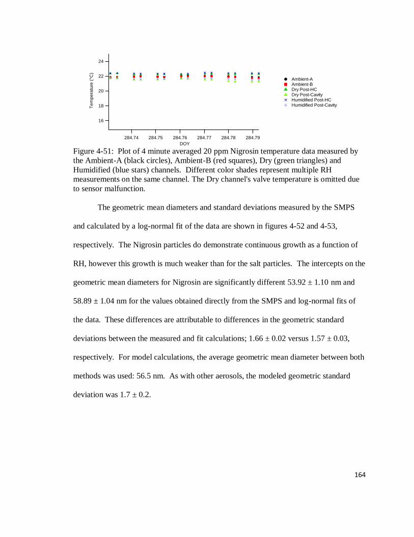
164
Figure 4-51: Plot of 4 minute averaged 20 ppm Nigrosin temperature data measured by
the Ambient-A (black circles), Ambient-B (red squares), Dry (green triangles) and
Humidified (blue stars) channels. Different color shades represent multiple RH
measurements on the same channel. The Dry channel's valve temperature is omitted due
to sensor malfunction.
The geometric mean diameters and standard deviations measured by the SMPS
and calculated by a log-normal fit of the data are shown in figures 4-52 and 4-53,
respectively. The Nigrosin particles do demonstrate continuous growth as a function of
RH, however this growth is much weaker than for the salt particles. The intercepts on the
geometric mean diameters for Nigrosin are significantly different 53.92 ± 1.10 nm and
58.89 ± 1.04 nm for the values obtained directly from the SMPS and log-normal fits of
the data. These differences are attributable to differences in the geometric standard
deviations between the measured and fit calculations; 1.66 ± 0.02 versus 1.57 ± 0.03,
respectively. For model calculations, the average geometric mean diameter between both
methods was used: 56.5 nm. As with other aerosols, the modeled geometric standard
deviation was 1.7 ± 0.2.
24
22
20
18
16
Te
mp
era
ture
(°C
)
284.79284.78284.77284.76284.75284.74
DOY
Ambient-A Ambient-B Dry Post-HC Dry Post-Cavity Humidified Post-HC Humidified Post-Cavity
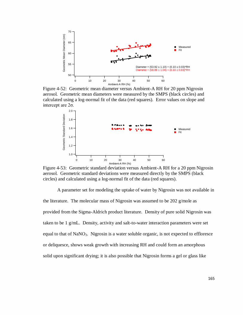
165
Figure 4-52: Geometric mean diameter versus Ambient-A RH for 20 ppm Nigrosin
aerosol. Geometric mean diameters were measured by the SMPS (black circles) and
calculated using a log-normal fit of the data (red squares). Error values on slope and
intercept are 2ζ.
Figure 4-53: Geometric standard deviation versus Ambient-A RH for a 20 ppm Nigrosin
aerosol. Geometric standard deviations were measured directly by the SMPS (black
circles) and calculated using a log-normal fit of the data (red squares).
A parameter set for modeling the uptake of water by Nigrosin was not available in
the literature. The molecular mass of Nigrosin was assumed to be 202 g/mole as
provided from the Sigma-Aldrich product literature. Density of pure solid Nigrosin was
taken to be 1 g/mL. Density, activity and salt-to-water interaction parameters were set
equal to that of NaNO3. Nigrosin is a water soluble organic, is not expected to effloresce
or deliquesce, shows weak growth with increasing RH and could form an amorphous
solid upon significant drying; it is also possible that Nigrosin forms a gel or glass like
70
65
60
55
50
Ge
om
etr
ic M
ea
n D
iam
ete
r (n
m)
6050403020100
Ambient-A RH (%)
Diameter = (53.92 ± 1.10) + (0.10 ± 0.03)*RHDiameter = (58.89 ± 1.04) + (0.10 ± 0.03)*RH
Measured Fit
2.0
1.8
1.6
1.4
1.2
1.0
Ge
om
etr
ic S
tan
da
rd D
evia
tio
n
6050403020100
Ambient-A RH (%)
Measured Fit
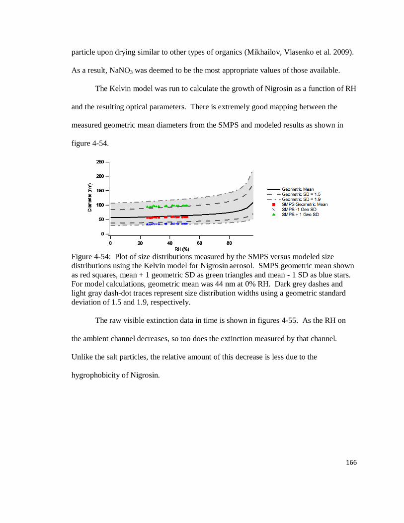
166
particle upon drying similar to other types of organics (Mikhailov, Vlasenko et al. 2009).
As a result, NaNO3 was deemed to be the most appropriate values of those available.
The Kelvin model was run to calculate the growth of Nigrosin as a function of RH
and the resulting optical parameters. There is extremely good mapping between the
measured geometric mean diameters from the SMPS and modeled results as shown in
figure 4-54.
Figure 4-54: Plot of size distributions measured by the SMPS versus modeled size
distributions using the Kelvin model for Nigrosin aerosol. SMPS geometric mean shown
as red squares, mean + 1 geometric SD as green triangles and mean - 1 SD as blue stars.
For model calculations, geometric mean was 44 nm at 0% RH. Dark grey dashes and
light gray dash-dot traces represent size distribution widths using a geometric standard
deviation of 1.5 and 1.9, respectively.
The raw visible extinction data in time is shown in figures 4-55. As the RH on
the ambient channel decreases, so too does the extinction measured by that channel.
Unlike the salt particles, the relative amount of this decrease is less due to the
hygrophobicity of Nigrosin.

167
Figure 4-55: Plot of 4 minute averaged 20 ppm Nigrosin extinction data measured in the
visible (532 nm) by the Ambient-A (black circles), Ambient-B (red squares), Dry (green
triangles) and Humidified (blue stars) channels.
Calculated f(RH) values using the Kelvin model and from the raw data are shown
in figure 4-56. The relative magnitude of change in extinction with RH is dampened
relative to all of the other particle types, including NaNO3. The model does a good job of
mapping f(RH) at lower RH, but is undercalculating f(RH) at higher RH. It is also
interesting to note that the orientation of the 1.5 and 1.9 geometric standard deviations are
reversed relative to all of the other particle types. For all of the salts, f(RH) increased
with decreasing geometric standard deviation, while it is increasing with increasing
geometric standard deviation here. This is most likely due to the absorbing character of
Nigrosin. As Nigrosin takes up water, the refractive index shifts towards that of water.
Absorption by the particle decreases and approaches a minimum limit as water uptake
occurs, however scattering by the particles increase due to increasing particle size. It
seems from this plot that the relative magnitude of the 2 processes (absorption decreasing
and scattering increasing) are approximately equal as seen by the small f(RH) values
measured.
100
80
60
40
20
0
Vis
Extin
ctio
n (
Mm
-1)
284.79284.78284.77284.76284.75284.74
DOY
Ambient-A Ambient-B Dry Humidified

168
Figure 4-56: Plot of f(RH) in the visible for the size distributions modeled in figure 4-54
using partial molar refraction. Geometric mean diameter was taken to be 44 nm. Dashed
dark gray line and dash-dot light gray line represent geometric standard deviations of 1.5
and 1.9 respectively. Lighter shading in between these 2 traces show the range of f(RH)
values calculated between these 2 limits. Solid black dot and blue stars are the Ambient-
A and Humidified channel visible f(RH) values calculated relative to the Dry channel,
respectively.
4.11.1. Calculation of Nigrosin refractive index at other wavelengths
Another caveat to modeling the change in optical properties of Nigrosin is that
values for the refractive index in the IR and UV have not been previously quantified, so a
value must be inferred. At 532 nm, the refractive index of Nigrosin has been reported as
1.70 (±0.04) + 0.31i (±0.05i) (Lack, Lovejoy et al. 2006). To derive an effective
refractive index for Nigrosin in the UV and IR, some mathematical manipulation was
necessary.
The imaginary term of the refractive index has been linked to the absorption by
the bulk (ABulk) (Bohren and Huffman 1983):
(eq 4-22)
where k is the imaginary part of the refractive index and λ is the wavelength. The
absorption of Nigrosin in the bulk was not performed, however an absorption spectrum of
a 20 ppm Nigrosin solution was collected as shown in figure 4-57.
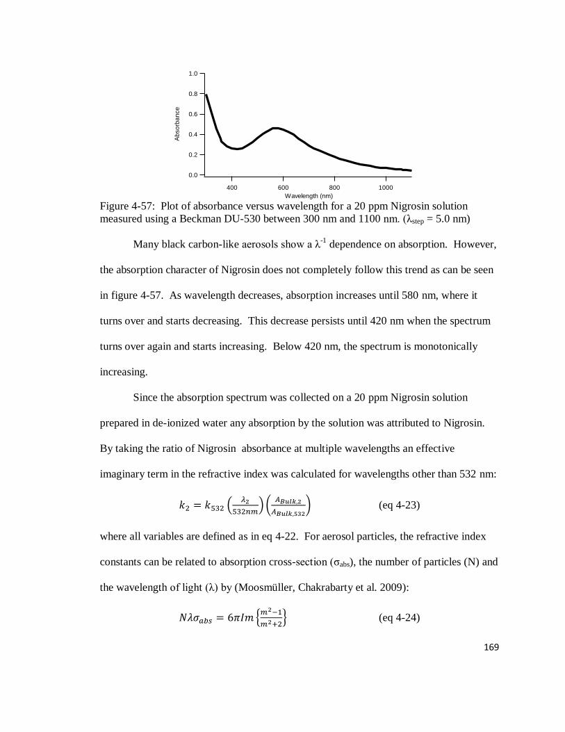
169
Figure 4-57: Plot of absorbance versus wavelength for a 20 ppm Nigrosin solution
measured using a Beckman DU-530 between 300 nm and 1100 nm. (λstep = 5.0 nm)
Many black carbon-like aerosols show a λ-1
dependence on absorption. However,
the absorption character of Nigrosin does not completely follow this trend as can be seen
in figure 4-57. As wavelength decreases, absorption increases until 580 nm, where it
turns over and starts decreasing. This decrease persists until 420 nm when the spectrum
turns over again and starts increasing. Below 420 nm, the spectrum is monotonically
increasing.
Since the absorption spectrum was collected on a 20 ppm Nigrosin solution
prepared in de-ionized water any absorption by the solution was attributed to Nigrosin.
By taking the ratio of Nigrosin absorbance at multiple wavelengths an effective
imaginary term in the refractive index was calculated for wavelengths other than 532 nm:
(eq 4-23)
where all variables are defined as in eq 4-22. For aerosol particles, the refractive index
constants can be related to absorption cross-section (ζabs), the number of particles (N) and
the wavelength of light (λ) by (Moosmüller, Chakrabarty et al. 2009):
(eq 4-24)
1.0
0.8
0.6
0.4
0.2
0.0A
bso
rba
nce
1000800600400
Wavelength (nm)

170
where m is the complex refractive index and Im stands for the imaginary portion of the
term in brackets. Here, N*ζabs was taken to be proportional to ABulk. It then follows from
eq 4-24 that
(eq 4-24)
where all terms are defined similarly to eq 4-24 and the subscripts denote wavelength.
Using equation 4-23 followed by equation 4-24, values for the real and imaginary terms
of the refractive index of Nigrosin in the IR and UV were determined to be 1.64 + 0.07i
and 1.69 + 0.17i, respectively; see table 4-12.
Table 4-12: Absorbance and imaginary refractive index versus wavelength for Nigrosin
solution at the 3 wavelengths used in the HC-CRDT
Wavelength (nm) A n k
1064 0.051 1.64 0.07
532 0.427 1.7 0.31
355 0.355 1.69 0.17
Plots of the measured UV extinction and f(RH) in the UV for the Nigrosin aerosol
are shown in figures 4-58 and 4-59, respectively. Unlike in the visible, the UV does not
show significant differentiation between the Humidified, Dry and Ambient channels.
This is most likely due to the decrease in strength when shifting to the UV from the
visible. This trend is mirrored in f(RH); all values are near 1. The modeling of f(RH) is
over calculating the value, but the general trend of very little increase in extinction with
RH is maintained. It is also possible that extinction in the UV by the humidified channel
is being under-measured as the clean air extinction was approximately 3750 Mm-1
.

171
Figure 4-58: Plot of 4 minute averaged 20 ppm Nigrosin data measured in the UV by the
Ambient-A (black circles), Ambient-B (red squares), Dry (green triangles) and
Humidified (blue stars) channels.
Figure 4-59: Plot of f(RH) in the UV for the size distributions modeled in figure 4-54
using partial molar refraction. Geometric mean diameter was taken to be 44 nm. Dashed
dark gray line and dash-dot light gray line represent geometric standard deviations of 1.5
and 1.9 respectively. Lighter shading in between these 2 traces show the range of f(RH)
values calculated between these 2 limits. Solid black dot and blue stars are the Ambient-
A and Humidified channel visible f(RH) values calculated relative to the Dry channel,
respectively.
Plots of the measured IR extinction and f(RH) in the IR for the Nigrosin aerosol
are shown in figures 4-60 and 4-61. Like with the UV, very little differentiation between
the Humidified, Dry and Ambient channels exists. This is most likely due to absorption
strength going towards 0 in the IR. Further, since growth of Nigrosin as a function of RH
is very weak, all f(RH); all values are near 1. The modeling of f(RH) is close to the
measured values. The absolute magnitudes of all measured values in the IR are close to
the LOQ for the HC-CRDT this is probably the most prominent source of error.
200
150
100
50
0
UV
Extin
ctio
n (
Mm
-1)
284.79284.78284.77284.76284.75284.74
DOY
Ambient-A Ambient-B Dry Humidified

172
Figure 4-60: Plot of 4 minute averaged 20 ppm Nigrosin data measured in the IR by the
Ambient-A (black circles), Ambient-B (red squares), Dry (green triangles) and
Humidified (blue stars) channels.
Figure 4-61: Plot of f(RH) in the IR for the size distributions modeled in figure 4-54
using partial molar refraction. Geometric mean diameter was taken to be 44 nm. Dashed
dark gray line and dash-dot light gray line represent geometric standard deviations of 1.5
and 1.9 respectively. Lighter shading in between these 2 traces show the range of f(RH)
values calculated between these 2 limits. Solid black dot and blue stars are the Ambient-
A and Humidified channel visible f(RH) values calculated relative to the Dry channel,
respectively.
20
15
10
5
0
IR E
xtin
ctio
n (
Mm
-1)
284.79284.78284.77284.76284.75284.74
DOY
Ambient-A Dry Humidified
173
5. Conclusions & Future Directions
The NephCam imaging system was optimized by imaging targets for astigmatism,
calibration dot matrices for distortion and coma, a white background for vignetting,
checkerboards for contrast and a white line on a black background to simulate the actual
diode laser's image shape. The 1.6 aperture on the camera was chosen because it allowed
for the most intensity, lack of astigmatism and coma as evidenced by the white
background and targets, respectively. But, relative to the larger aperture settings, the 1.6
aperture must be corrected for the effects of vignetting; image intensity drops off as cos4
from center. The 1.6 aperture also has less total contrast across an image - 0.3 for the 1.6
aperture versus 1 for the 8 aperture - but the 1.6 aperture was preferable because the
contrast was constant across an image as seen by the modular transfer functions. While it
is possible to correct for the effects of vignetting, it is not possible to correct for changes
in contrast.
A model was developed to link theoretical image shape to those actually captured
by the NephCam. The model was based entirely upon ray tracing methods and all
physical parameters of the camera system were considered. When considering only a
single size of particle, model and image shapes do not agree very well. However, the
inclusion of multiple charge-to-size effects present from the DMA's sizing mechanism
improved agreement significantly. Finally, the inclusion of contrast effects from the 1.6
aperture - contrast is only 30% - resulted in further improvement in agreement between
modeled and actual image shapes.
The NephCam was calibrated as a function of particle size for AS aerosols. The
HC-CRDT was operated in tandem to generate scattering coefficients; absorption for AS

174
is negligible so extinction and scattering are equivalent. Because of the multiple charge-
to-size effects from the DMA, smaller particle diameters required a 2nd order polynomial
calibration curve instead of a linear one. In this size regime, the measured scattering
coefficients increases faster than measured peak amplitudes. However, as base particle
size increased above 400 nm the magnitude of the non-linear effects decreased to 0. In
this size regime, the relative increase in scattering versus peak amplitude goes towards 1
as a result of camera collection angles and collection efficiency. Also, size-selected
particles with base diameters 700 nm or larger do not exhibit multiple charge-to-size
effects because of the 1μm impactor on the DMA; these particles are removed by
impaction. The SSA of size selected Nigrosin particles was calculated and good
agreement was observed at larger particle sizes. At smaller particle sizes the multiple
charge-to-size effect caused the SSA to be over measured.
Relative humidity dependent extinction coefficients of various water soluble
particles were measured: AS, NaNO3, NaCl and Nigrosin. The effect of water uptake on
the measured extinction coefficients was modeled using the Kelvin equation and 3
refractive index mixing rules: volume, Maxwell-Garnett and partial molar refraction.
Good agreement between modeled results and actual data were observed for all of the salt
particles except in the UV of the humidified channel. This disagreement stems from the
measured extinction on this channel being too high to accurately measure values. Less
agreement between the Nigrosin measured and modeled data was obtained as a result of
inferring Nigrosin's water uptake behavior; it was assumed to behave identically to
NaNO3. Also, the absorbing character of Nigrosin could be affecting these values since
effective refractive indices were inferred from the mixing rules. While all 3 mixing rules

175
worked well for the non-absorbing salts they may not be as appropriate for absorbing
species. In the future, this disagreement should be revisited with the inclusion of a
scattering measurement; a single NephCam would not have given enough information, so
only extinction was measured.
In moving forward with the NephCams a better algorithm for extracting the
underlying particle size from image shape must be extracted. Shape effects in the images
arise from higher order Bessel terms being present when light interacts with a particle.
A similar situation is true with atomic orbitals; as atoms increase in size, the number of
available orbitals increases and the shape of the orbitals change depending upon type (i.e.
S, P, D, F). My thoughts toward extracting size information a priori from the image
shape is that the NephCam will have to be trained to extract the convolution of Bessel
functions from a set of particles; Principle Component Analysis is the most likely
scheme. The speed of data collection by the cameras must be increased so that the
extraction of this type of information is possible. The large number of particles being
measured with a 10 sec exposure time makes this extraction physically impossible.
Extending NephCam usage to all 4 channels of the HC-CRDT will help with this problem
to some extent as changes in scattering as a function of RH should help in the derivation
of size and refractive index of particles on the dry channel.
In moving forward with the HC-CRDT, more data needs to be collected. Some
small problems, like vibration sensitivity and clean air baselines, need to be addressed.
But, the instrument is ready to collect humidification data on many different particles
types; specifically carbonaceous and ambient aerosols. Currently, a wood-burner is being
developed in our lab to examine the optical properties of different types of smoldering

176
wood combustion as a function of RH. The measurement of ambient aerosols using the
HC-CRDT will allow for the elucidation of particle growth and transformation
mechanisms which is currently a point of intense research among the aerosol community.
Instrument inter-comparisons are also of interest to validate the HC-CRDT.
177
6. References
Andreae, M. O. and A. Gelencser (2006). "Black carbon or brown carbon? The nature of light-absorbing carbonaceous aerosols." Atmos. Chem. Phys. 6(10): 3131-3148.
Andrews, E., P. J. Sheridan, et al. (2004). "In situ aerosol profiles over the Southern Great Plains cloud and radiation test bed site: 1. Aerosol optical properties." J. Geophys. Res. 109(D6): D06208.
Anttila, T., V. M. Kerminen, et al. (2004). "Modelling the formation of organic particles in the atmosphere." Atmos. Chem. Phys. 4(4): 1071-1083.
Atkinson, D. B. (2003). "Solving chemical problems of environmental importance using cavity ring-down spectroscopy." The Analyst 128(2): 117 - 125.
Baltensperger, U., L. Barrie, et al. (2003). WMO/GAW Aerosol Measurement Procedures: Guidelines and Recommendations. WMO. Geneva.
Bergstrom, R. W., P. Pilewskie, et al. (2007). "Spectral absorption properties of atmospheric aerosols." Atmos. Chem. Phys. 7(23): 5937-5943.
Bergstrom, R. W., P. B. Russell, et al. (2002). "Wavelength Dependence of the Absorption of Black Carbon Particles: Predictions and Results from the TARFOX Experiment and Implications for the Aerosol Single Scattering Albedo." Journal of the Atmospheric Sciences 59(3): 567-577.
Biskos, G., A. Malinowski, et al. (2006). "Nanosize Effect on the Deliquescence and the Efflorescence of Sodium Chloride Particles." Aerosol Science and Technology 40(2): 97-106.
Biskos, G., D. Paulsen, et al. (2006). "Prompt deliquescence and efflorescence of aerosol nanoparticles." Atmos. Chem. Phys. 6(12): 4633-4642.
Biskos, G., L. M. Russell, et al. (2006). "Nanosize effect on the hygroscopic growth factor of aerosol particles." Geophys. Res. Lett. 33(7): L07801.
Bohren, C. F. and D. R. Huffman (1983). Absorption and scattering of light by small particles. New York, Wiley.
Bond, T. C. and R. W. Bergstrom (2006). "Light absorption by carbonaceous particles: An investigative review." Aerosol Science and Technology 40(1): 27-67.
Bond, T. C., M. Bussemer, et al. (1999). "Light Absorption by Primary Particle Emissions from a Lignite Burning Plant." Environmental Science & Technology 33(21): 3887-3891.
Bond, T. C., G. Habib, et al. (2006). "Limitations in the enhancement of visible light absorption due to mixing state." J. Geophys. Res. 111(D20): D20211.
Bueno, P. A., D. K. Havey, et al. (2011). "Photoacoustic Measurements of Amplification of the Absorption Cross Section for Coated Soot Aerosols." Aerosol Science and Technology 45(10): 1217-1230.
Bulatov, V., M. Fisher, et al. (2002). "Aerosol analysis by cavity-ring-down laser spectroscopy." Analytica Chimica Acta 466(1): 1-9.
Campbell, D., S. Copeland, et al. (1995). "Measurement of Aerosol Absorption Coefficient from Teflon Filters Using Integrating Plate and Integrating Sphere Techniques." Aerosol Science and Technology 22(3): 287-292.
Carrico, C. M., P. Kus, et al. (2003). "Mixtures of pollution, dust, sea salt, and volcanic aerosol during ACE-Asia: Radiative properties as a function of relative humidity." J. Geophys. Res. 108(D23): 8650.
Chen, Y. and T. C. Bond (2009). "Light absorption by organic carbon from wood combustion." Atmos. Chem. Phys. Discuss. 9(5): 20471-20513.

178
Chyýlek, P., V. Srivastava, et al. (1988). "Scattering of electromagnetic waves by composite spherical particles: experiment and effective medium approximations." Appl. Opt. 27(12): 2396-2404.
Core Writing Team, P., R.K. and Reisinger, A. (Eds.) (2007). Contribution of Working Groups I, II and III to the Fourth Assessment Report of the Intergovernmental Panel on Climate Change. Climate Change 2007: Synthesis Report Geneva, Switzerland, IPCC: 104.
Cox, A. (1966). Photographic Optics: A modern approach to the technique of definition. London & New York, Focal Press.
De Haan, D. O., T. Brauers, et al. (1999). "Heterogeneous chemistry in the troposphere: Experimental approaches and applications to the chemistry of sea salt particles." International Reviews in Physical Chemistry 18(3): 343-385.
Dutcher, C. S., A. S. Wexler, et al. (2010). "Surface Tensions of Inorganic Multicomponent Aqueous Electrolyte Solutions and Melts." The Journal of Physical Chemistry A 114(46): 12216-12230.
Eck, T., P. Bhartia, P. Hwang, and L. Stowe (1987). "Reflectivity of Earth's Surface and Clouds in Ultraviolet From Satellite Observations." J. Geophys. Res. 92(D4): 4287-4296.
Erlick, C., J. P. D. Abbatt, et al. (2011). "How Different Calculations of the Refractive Index Affect Estimates of the Radiative Forcing Efficiency of Ammonium Sulfate Aerosols." Journal of the Atmospheric Sciences 68(9): 1845-1852.
Everest, M. A. and D. B. Atkinson (2008). "Discrete sums for the rapid determination of exponential decay constants." Review of Scientific Instruments 79(2): 023108-023109.
Fierz, M. (2005). LabView Mie Scattering Program. Finlayson-Pitts, B. J. and J. James N. Pitts (2000). Chemistry of the upper and lower
atmosphere: Theory, Experiments and Applications. San Diego, CA, Academic Press. Freedman, A. (2009). Allan Variance Igor Macro. Freney, E. J., S. T. Martin, et al. (2009). "Deliquescence and Efflorescence of Potassium Salts
Relevant to Biomass-Burning Aerosol Particles." Aerosol Science and Technology 43(8): 799-807.
Frost, R. (1916). Mountain interval. New York, H. Holt and company. Gelencser, A., A. Hoffer, et al. (2000). "Thermal behaviour of carbonaceous aerosol from a
continental background site." Atmospheric Environment 34(5): 823-831. Gysel, M., E. Weingartner, et al. (2001). "Hygroscopicity of Aerosol Particles at Low
Temperatures. 2. Theoretical and Experimental Hygroscopic Properties of Laboratory Generated Aerosols." Environmental Science & Technology 36(1): 63-68.
Hämeri, K., A. Laaksonen, et al. (2001). "Hygroscopic growth of ultrafine sodium chloride particles." J. Geophys. Res. 106(D18): 20749-20757.
Heintzenberg, J., A. Wiedensohler, et al. (2006). "Intercomparisons and Aerosol Calibrations of 12 Commercial Integrating Nephelometers of Three Manufacturers." Journal of Atmospheric and Oceanic Technology 23(7): 902-914.
Hoffer, A., A. Gelencser, et al. (2005). "Optical properties of humic-like substances (HULIS) in biomass-burning aerosols." Atmos. Chem. Phys. Discuss. 5(4): 7341-7360.
Hoffman, R. C., A. Laskin, et al. (2004). "Sodium nitrate particles: physical and chemical properties during hydration and dehydration, and implications for aged sea salt aerosols." Journal of Aerosol Science 35(7): 869-887.
179
Horvath, H. (1993). "Atmospheric light absorption--A review." Atmospheric Environment. Part A. General Topics 27(3): 293-317.
Kirchstetter, T. W., T. Novakov, et al. (2004). "Evidence that the spectral dependence of light absorption by aerosols is affected by organic carbon." J. Geophys. Res. 109.
Knutson, E. O. and K. T. Whitby (1975). "Aerosol classification by electric mobility: apparatus, theory, and applications." Journal of Aerosol Science 6(6): 443-451.
Koren, I., Y. J. Kaufman, et al. (2004). "Measurement of the Effect of Amazon Smoke on Inhibition of Cloud Formation." Science 303(5662): 1342-1345.
Kotchenruther, R. A., P. V. Hobbs, et al. (1999). "Humidification factors for atmospheric aerosols off the mid-Atlantic coast of the United States." J. Geophys. Res. 104(D2): 2239-2251.
Krämer, L., U. Pöschl, et al. (2000). "Microstructural rearrangement of sodium chloride condensation aerosol particles on interaction with water vapor." Journal of Aerosol Science 31(6): 673-685.
Kulmala, M., L. Laakso, et al. (2004). "Initial steps of aerosol growth." Atmos. Chem. Phys. 4(11/12): 2553-2560.
Lack, D. A. and C. D. Cappa (2010). "Impact of brown and clear carbon on light absorption enhancement, single scatter albedo and absorption wavelength dependence of black carbon." Atmos. Chem. Phys. 10(9): 4207-4220.
Lack, D. A., E. R. Lovejoy, et al. (2006). "Aerosol Absorption Measurement using Photoacoustic Spectroscopy: Sensitivity, Calibration, and Uncertainty Developments." Aerosol Science and Technology 40(9): 697 - 708.
Lee, K. O., R. Cole, et al. (2002). "Morphological investigation of the microstructure, dimensions, and fractal geometry of diesel particulates." Proceedings of the Combustion Institute 29(1): 647-653.
Levin, E. J. T., G. R. McMeeking, et al. (2010). "Biomass burning smoke aerosol properties measured during Fire Laboratory at Missoula Experiments (FLAME)." J. Geophys. Res. 115(D18): D18210.
Lewis, E. R. and S. E. Schwartz (2004). Sea salt aerosol production: mechanisms, methods, measurements and models - a critical review. Washington, DC, American Geophysical Union.
Lewis, K. A., W. P. Arnott, et al. (2009). "Reduction in biomass burning aerosol light absorption upon humidification: roles of inorganically-induced hygroscopicity, particle collapse, and photoacoustic heat and mass transfer." Atmos. Chem. Phys. 9(22): 8949-8966.
Lohmann, U. and J. Feichter (2005). "Global indirect aerosol effects: a review." Atmos. Chem. Phys. 5(3): 715 - 737.
Mathis, U., M. Mohr, et al. (2005). "Influence of Diesel Engine Combustion Parameters on Primary Soot Particle Diameter." Environmental Science & Technology 39(6): 1887-1892.
Mayol-Bracero, O. L., P. Guyon, et al. (2002). "Water-soluble organic compounds in biomass burning aerosols over Amazonia 2. Apportionment of the chemical composition and importance of the polyacidic fraction." J. Geophys. Res. 107(D20): 8091.
Mikhailov, E., S. Vlasenko, et al. (2009). "Amorphous and crystalline aerosol particles interacting with water vapor: conceptual framework and experimental evidence for restructuring, phase transitions and kinetic limitations." Atmos. Chem. Phys. 9(24): 9491-9522.

180
Milford, J. B. and C. I. Davidson (1985). "The sizes of particulate trace elements in the atmosphere--a review." Journal of the Air Pollution Control Association 35(12): 1249-1260.
Mirabel, P. (2000). "A theory for the deliquescence of small particles." J. Chem. Phys. 113(18): 8200.
Moosmüller, H., R. K. Chakrabarty, et al. (2009). "Aerosol light absorption and its measurement: A review." Journal of Quantitative Spectroscopy and Radiative Transfer 110(11): 844-878.
Moosmuller, H., R. Varma, et al. (2005). "Cavity ring-down and cavity-enhanced detection techniques for the measurement of aerosol extinction." Aerosol Science and Technology 39(1): 30-39.
Müller, T., A. Nowak, et al. (2009). "Angular Illumination and Truncation of Three Different Integrating Nephelometers: Implications for Empirical, Size-Based Corrections." Aerosol Science and Technology 43(6): 581-586.
Pan, X. L., P. Yan, et al. (2009). "Observational study of aerosol hygroscopic growth factors over rural area near Beijing mega-city." Atmos. Chem. Phys. Discuss. 9(1): 5087-5118.
Poschl, U. (2005). "Atmospheric aerosols: Composition, transformation, climate and health effects." Angewandte Chemie-International Edition 44(46): 7520-7540.
Pöschl, U. (2003). "Aerosol particle analysis: challenges and progress." Analytical and Bioanalytical Chemistry 375(1): 30-32.
Reid, J. S., J. E. Kinney, et al. (2003). "Analysis of measurements of Saharan dust by airborne and ground-based remote sensing methods during the Puerto Rico Dust Experiment (PRIDE)." J. Geophys. Res. 108(D19): 8586.
Schnaiter, M., H. Horvath, et al. (2003). "UV-VIS-NIR spectral optical properties of soot and soot-containing aerosols." Journal of Aerosol Science 34(10): 1421-1444.
Schwartz, S. E. (1996). "The whitehouse effect--Shortwave radiative forcing of climate by anthropogenic aerosols: an overview." Journal of Aerosol Science 27(3): 359-382.
Sihvola, A. (2008). Electromagnetic mixing formulas and applications. London, Institution of Electrical Engineers.
Slowik, J. G., E. S. Cross, et al. (2007). "Measurements of Morphology Changes of Fractal Soot Particles using Coating and Denuding Experiments: Implications for Optical Absorption and Atmospheric Lifetime." Aerosol Science and Technology 41(8): 734-750.
Stanier, C. O., R. K. Pathak, et al. (2007). "Measurements of the Volatility of Aerosols from α-Pinene Ozonolysis." Environmental Science & Technology 41(8): 2756-2763.
Stelson, A. W. (1990). "Urban aerosol refractive index prediction by partial molar refraction approach." Environmental Science & Technology 24(11): 1676-1679.
Subramanian, R., C. A. Roden, et al. (2007). "Yellow Beads and Missing Particles: Trouble Ahead for Filter-Based Absorption Measurements." Aerosol Science and Technology 41(6): 630 - 637.
Sun, H., L. Biedermann, et al. (2007). "Color of brown carbon: A model for ultraviolet and visible light absorption by organic carbon aerosol." Geophys. Res. Lett. 34.
Tang, I. N. (1976). "Phase transformation and growth of aerosol particles composed of mixed salts." Journal of Aerosol Science 7(5): 361-371.
Tang, I. N. (1996). "Chemical and size effects of hygroscopic aerosols on light scattering coefficients." J. Geophys. Res. 101(D14): 19245-19250.

181
Tang, I. N. and H. R. Munkelwitz (1994). "Water activities, densities, and refractive indices of aqueous sulfates and sodium nitrate droplets of atmospheric importance." J. Geophys. Res. 99(D9): 18801-18808.
Taubman, B. F., L. T. Marufu, et al. (2004). "Smoke over haze: Aircraft observations of chemical and optical properties and the effects on heating rates and stability." J. Geophys. Res. 109(D2): D02206.
Toon, O. B., J. B. Pollack, et al. (1976). "The Optical Constants of Several Atmospheric Aerosol Species: Ammonium Sulfate, Aluminum Oxide, and Sodium Chloride." J. Geophys. Res. 81(33): 5733-5748.
Toscano, G., I. Moret, et al. (2011). "Distribution and seasonal variability of trace elements in atmospheric particulate in the Venice Lagoon." Chemosphere 85(9): 1518-1524.
Wayne, R. P. (1996). Chemistry of Atmospheres. Oxford, Oxford University Press. Yang, M., S. G. Howell, et al. (2008). "Attribution of aerosol light absorption to black carbon,
brown carbon, and dust in China; interpretations of atmospheric measurements during EAST-AIRE." Atmos. Chem. Phys. Discuss. 8(3): 10913-10954.
Zhang, R., A. F. Khalizov, et al. (2008). "Variability in morphology, hygroscopicity, and optical properties of soot aerosols during atmospheric processing." Proceedings of the National Academy of Sciences 105(30): 10291-10296.
Zhang, R., I. Suh, et al. (2004). "Atmospheric New Particle Formation Enhanced by Organic Acids." Science 304(5676): 1487-1490.