biblio.ugent.be

The UGent Institutional Repository is the electronic archiving and dissemination platform for all UGent research

publications. Ghent University has implemented a mandate stipulating that all academic publications of UGent

researchers should be deposited and archived in this repository. Except for items where current copyright

restrictions apply, these papers are available in Open Access.

This item is the archived peer-reviewed author-version of:

Development of a coupled CFD-HAM model including liquid moisture transport to study

moisture transport in building materials

Van Belleghem M., De Backer L., Janssens A., De Paepe M.

In: Proceedings of the 5th

International Building Physics Conference, Kyoto, Japan 28 May – 31 May

2012, IBPC5.

Optional: link to the article

To refer to or to cite this work, please use the citation to the published version:

Van Belleghem M., De Backer M., Janssens A., De Paepe M. Development of a coupled CFD-HAM

model including liquid moisture transport to study moisture transport in building materials.

Proceedings of the 5th

International Building Physics Conference, IBPC5, Kyoto University, Kyoto,

Japan, 2012

Development of a coupled CFD-HAM model including liquid moisture transport to study moisture transport in building materials

Marnix Van Belleghem1, Lien De Backer2, Arnold Janssens2 and Michel De Paepe1

1Department of Flow, Heat and Combustion Mechanics, Ghent University, Ghent, Belgium 2Department of Architecture and Urban Planning, Ghent University, Ghent, Belgium

Keywords: HAM, CFD, modelling, drying, hygroscopic, capillary active

ABSTRACT

Heat and moisture transport in buildings have a large impact on the building envelope durability, the energy use in buildings and the indoor climate. Nowadays HAM (Heat, Air and Moisture) models are widely used to simulate and predict the effect of these transport phenomena in detail. Recently these HAM models are being coupled to CFD (Computational Fluid Dynamics) to study the moisture exchange between air and porous materials on a local scale (microclimates). A direct coupling approach between CFD and HAM is applied. The transport equations for heat and moisture in a porous material are directly implemented into an existing CFD package and the transport equations in the air and in the porous material can be solved in the same iteration by only one solver. In this paper an existing model for moisture transport in the hygroscopic range is extended to also incorporate liquid moisture transport. This way a broader range of problems can be tackled such as drying phenomena and interstitial condensation in building components. The material model is validated using a drying experiment on ceramic brick. Further development of the model should allow a direct coupling of the heat and moisture transported in the material and the air surrounding the material.

1. Introduction

Moisture in porous building materials can give rise to all kinds of damage phenomena such as frost damage, salt crystallisation and mould growth. At the same time moisture in building envelopes can have a negative impact on insulation values and increase the energy use of buildings. Therefore a detailed knowledge of the moisture transport in these porous materials is important. Modelling the heat and moisture transport can help in understanding the mechanisms which are of importance.

In literature a lot of modelling approaches are found which can often be related to the work of Philip and de Vries (1957) and Whitaker (1977). Philip and de Vries proposed a diffusion approach on a macroscopic level. This phenomenological approach considered the porous material as a continuous medium. Whitaker on the other hand made a more fundamental approach and started from the discrete phases in the porous material (solid, liquid, gas). He then averaged these equations to result again in a lumped model. Although this approach is more complex, it gives more insight in the porous material behaviour and the assumptions that are made during the modelling.

Different transported scalars are used in the different transport models and generally two approaches can be found: a diffusivity approach and a permeability approach (Carmeliet et al. 2001). In the diffusivity approach the moisture content is used as the transported property while the permeability approach uses capillary pressure (which is related to the moisture content through the retention curve). Berger et al. (1973) for example developed a numerical model for drying using a diffusivity approach. Examples of permeability approaches are found in Janssen (2007) and Grunewald (1997).

Coupling of these models with the moisture transport in the surrounding air is often realised by using convective transfer coefficients. This approach lumps the effects of the heat and moisture boundary layer into transfer coefficients. Often, for reasons of simplicity, these coefficients are assumed constant in time and space. Studies however showed that assuming a constant transfer coefficient can result in large errors (Defraeye 2011, Steeman 2009a and Steskens 2009). Also these transfer coefficients are often difficult to determine experimentally and the analytical formulation found in literature do not always apply.

Computational Fluid Dynamics (CFD) solves the boundary layer directly. If the heat and moisture transport model could be coupled with CFD in a direct manner, there would be no longer a need for transfer coefficients. Therefore a coupling strategy has to be implemented.

A previous study (Steeman 2009b) showed that it is possible to use the mass fraction of water vapour (kg vapour/ kg moist air) as the transported variable both in the air and in the porous material when moisture transport is studied in the hygroscopic range. This allowed a direct coupling of the transport equations in the air and in the material. When modelling in the over-hygroscopic range, relative humidity can be near to 100% and the vapour mass fraction is near the saturation value. This implies that a drop in temperature would result in a drop in vapour mass fraction since the mass fraction can not be higher than the saturation mass fraction. In other words, the mass fraction would become temperature dependant and this dependency results in numerical difficulties.

In this paper the heat and moisture transport in the porous material is therefore modelled by using the capillary pressure as the transported variable. The drawback of this model is that information at the boundary of the material can not be passed directly to the air side but has to be translated to a heat and mass flux leaving or going into the material. This coupling strategy will not be discussed in this paper. The paper will focus on the validation of the transport model in the porous material. The coupling of the material model with transport in the air is still ongoing research and will not be discussed in detail here.

2. Heat and moisture transport model

For reasons of completeness this section will discuss the combined heat and moisture transport model in a porous material and as well as in air.

When looking at porous materials generally used in buildings, three phases will be present: • Gas phase: air and water vapour • Liquid phase: liquid water • Solid phase: material matrix

In theory it is possible to model the different phases separately on a micro scale and subsequently integrate over the total material volume to obtain the macro scale heat and moisture transport (Whitaker 1977). This would however require such a detailed knowledge of the pore structure of the material that this approach is not feasible for materials encountered in practice. Therefore a phenomenological approach on a macro scale (Philip and de

Vries 1957) was used for the derivation of the transport equations. In these transport equations the material is considered to be a continuum. By consequence macro heterogenic effects like cracks can not be simulated while the effects of micro heterogeneities are averaged over the calculation element.

Two conservation equations are deduced and solved: conservation of mass and conservation of energy. The conservative property for mass in the air is the water vapour density ρvap (kg/m³) (the amount of moisture contained per air volume). The conserved property for mass in a porous material is the moisture content w (kg/m³). The conserved property for energy conservation is the total energy E (J). First the moisture and energy transfer equations in air are deduced, then similar equations for a porous material are formulated.

2.1 Moisture transport in air

Moisture is transported in air through a combination of convection and diffusion. In the air no liquid moisture is transported only water vapour. The water vapour diffusion flux is represented by g (kg/m²s) and is assumed proportional to the gradient of the water vapour mass fraction. Deff (m²/s) is the sum of the molecular and turbulent vapour diffusion coefficient (Eq. (1)).

turb

turbturb

va

turbvaeff

ScD

T

pxD

DDD

ν=

=

+=

−81.1

5

16.273

1013251031.2

(1)

In these equations Dva (m²/s) is the molecular diffusion coefficient and Dturb (m²/s) is the turbulent diffusion coefficient. p (Pa) is the operating pressure and T the temperature (K). The molecular diffusion coefficient is a property of the air-water vapour mixture only, while the turbulent diffusion coefficient is a property of the mixture and the flow. This turbulent diffusion coefficient is given as the ratio of the turbulent kinematic viscosity ν (m²/s) to the turbulent Schmidt number Sc(-). The value used for the turbulent Schmidt number is 0.7.

The water vapour density in the air can be expressed as the product of mass fraction of water vapour in the air Y (kgv/kga+v) and the total density of the moist air ρa+v.

Yvav += ρρ (2)

The density of the air is assumed independent of the pressure. In other words, the air is modeled as incompressible. This is an acceptable assumption since the encountered air velocities in buildings are low and much smaller than the speed of sound. Sorensen (2003) stated that the airflow in buildings can always be assumed incompressible. However the density does depend on temperature and vapour concentrations. To take the temperature dependence into account often the so called Boussinesq approximation is used. In this approach the density is taken as a constant in all solved equations except in the buoyancy term of the momentum equation where a linear relation between temperature and density is used. As a result of these simplifications the Boussinesq approximation is only valid for small temperature differences. However this model does not take into account the effect of water vapour concentration changes on the air density. Therefore a different approach is suggested, based on the incompressible ideal gas model. In this approach the influence of the temperature and concentration variation on the density is included in all transport equations, while the effect of pressure variations is neglected. The density is calculated with Eq. (3).

−+=+

av

va

M

Y

M

YRT

p

1ρ (3)

Here R is the universal gas constant (J/molK), Mv and Ma the molar weight of vapour and dry air respectively (kg/mol).

Eq. (4) shows the transport equation for water vapour in air in its divergence form. As mentioned before this transfer is governed by a convection term (second term on the left hand side) and a diffusion term (right hand side term). The first term on the left hand side represents the moisture storage in the air (moisture content change in time).

( ) ( ) ( )YDgYvt

Yeffvava

va ∇∇=−∇=∇+∂

∂++

+ ρρρ...

rr (4)

2.2 Heat transport in air

In air the energy transport equation can be written as a combination of storage, convection and diffusion of latent and sensible heat. This results in the following equation for the energy balance in the air:

( ) ( )[ ]( ) ( )( )[ ]

[ ] ( )( )[ ]gTCLTCT

TCYLTCYv

TCYLTCYt

airvapeff

airavvapav

airavvapav

r

r

−+∇−∇∇

=−++∇

+−++∂∂

++

++

..

1.

1

λρρ

ρρ (5)

In this equation Cv (J/kgK) is the heat capacity of water vapour and Ca (J/kgK) the heat capacity of air, T (K) is the temperature, v is the air velocity and λeff (W/mK) is the effective heat conductivity. The effective heat conductivity is the sum of the molecular heat conductivity λ and the turbulent conductivity λturb. The turbulent conductivity is calculated from the turbulent kinematic viscosity νturb and the turbulent Prandtl number with Eq. (6).

turbeff

turb

turbvaturb C

λλλ

νρλ

+=

= + Pr (6)

For the temperature ranges encountered in this work the latent heat of water vapour can be assumed constant. With this assumption and applying the conservation of mass equation, Eq.(5) simplifies to:

( ) ( )[ ]( )[ ]TgCCT

CTvt

CT

airvapeff

avav

r

r

−−∇∇

=∇+∂

∂+

+

λ

ρρ

.

. (7)

The mass weighted average heat capacity C is given by Eq. (8).

airvap CYYCC )1( −+= (8)

The following values have been used for the different material properties: Cv= 1875.2 J/kgK, Ca= 1006.43 J/kgK, λ= 0.0257 W/mK, Prturb= 0.85.

2.3 Moisture transport in porous material

Applying the conservation of mass principle for water to a control volume in a porous material results in stating that water entering a control volume through its boundary can either be stored in that control volume or leaves the volume again through its boundary. In differential from this gives us:

gt

w r.−∇=

∂∂

(9)

In words: the divergence of the moisture flux equals the change of the moisture content in time. Convective moisture transport is neglected.

It is assumed that moisture can be present in two phases: liquid moisture and water vapour. In other words, transport of moisture through a system is due to liquid moisture transport and water vapour transport and the moisture can be stored in a system in liquid and vapour phase. The sum of liquid water and water vapour gives the total moisture content w (kg/m³). Here it is assumed that the water vapour stored in a porous material is negligible compared to the stored liquid water.

Vapour transport in a porous material is described by Fick’s law for water vapour diffusion. According to Janssen (2011) the vapour diffusion flux gv (kg/m²s) is best described by the gradient of vapour pressure pv (Pa) as a driving force.

vv

vav p

TR

Dg ∇=

µr (10)

In this equation Dva (m²/s) is again the molecular diffusion coefficient of water vapour in air. µ (-) is the water vapour resistance factor which is the ratio of the water vapour diffusion coefficient in still air to the diffusion coefficient in the porous material.

Liquid moisture transport is described by Darcy’s law:

cll pKg ∇−=r (11)

Here Kl (s) is the liquid permeability and pc (Pa) is the capillary pressure and gl the liquid water flux (kg/m²s).

The vapour pressure pv can be transformed to the capillary pressure using Eqs. (12)-(14) and Kelvin’s law (Eq. (15)), which relates the capillary pressure to the relative humidity RH (-).

sat

v

p

pRH = (12)

( )

−−=

97.38

15.27308.17exp611

T

Tpsat

(13)

YRYRR

YpRp

ava

vv −+

= (14)

RHTRp vlc lnρ= (15)

psat is the saturation vapour pressure and is temperature dependant. Rv (J/kgK) and Ra (J/kgK) are the specific gas constants for vapour and air respectively, ρl is the density of liquid water (998 kg/m³).

Applying Eqs. (12)-(15) to Fick’s law results in the following equation for the vapour flux:

∇

∂∂+

∂∂+∇

∂∂−= T

T

pRH

T

RHpp

p

RHp

TR

Dg sat

satcc

satv

vav µr (16)

Combining Eq. (11) and (16) in Eq. (9) results in the conservation equation for mass transport in a porous material with the capillary pressure as transported variable:

∇

∂∂

+∂

∂+

∇+∇∇=

∂∂

∂∂

TT

pRH

T

RHp

pTR

DpK

t

p

p

w

satsat

cvl

vvacl

c

c

ρρ

µ. (17)

2.4 Heat transport in porous materials

No convective transport is assumed inside the porous material, only diffusion of moisture. This means that energy is only transported due to diffusion which results in Eq.(18).

hqt

E r.∇=

∂∂

(18)

Here qh is the total heat flux (W/m²). This total heat flux has three contributions: a heat flux due to heat conduction in the porous material, a heat flux due to vapour diffusion though the porous material and a heat flux due to liquid moisture transport. The total energy E is the sum of the energy stored in the solid porous material matrix, the energy stored in the liquid moisture phase and the energy stored in the water vapour phase. Applying these assumptions to Eq. (18) results in the heat transfer equation for a porous material:

( ) ( )( )[ ]vvllmat

vv

llvvllmatmat

gLTCgTCTt

wLTC

t

wTC

t

TCwCwC

t

E

rr +−−∇∇

=∂

∂++∂

∂+∂∂++

=∂∂

λ

ρ

.

(19)

In this equation λmat (W/mK) is the heat conductivity of the porous material. This conductivity is a function of the moisture content of the porous material since moisture contained inside the porous material would result in

an increase of the conductivity. ρmat (kg/m³) is the density of the porous material and Cmat is the heat capacity of the porous material. L is the latent heat of evaporation and is taken as a constant (2.5e6 J/kg). Cv and Cl are the heat capacities of vapour and liquid water respectively and are again assumed constant (Cv= 1875.2 J/kgK, Cl= 4192.1 J/kgK).

The total moisture content w (kg/m³) can by divided into the liquid moisture content wl and the vapour moisture content wv. Both are linked with the total moisture content through the open porosity ψ (-).

vl

vl

w

w

ρρ

ρψ

11 −

−=

vl

lv

w

w

ρρ

ψρ

11 −

−=

(20)

3. Verification of vapour transport modelling in a porous material

Milly (1982) presented an analytical solution to a vapour transport problem. This solution is used here for the verification of the vapour transport model. The same case was also used with succes by Janssen (2007), Steeman et al. (2009) and Steeman et al. (2010).

The considered test case of Milly (1982) represents the one dimensional, coupled diffusion of heat and water vapour in a 10 cm high porous material. Initially the temperature in the material is 20°C and the relative humidity is 23.87%. A step change is imposed at the top of the material: the relative humidity changes to 27.59% while the temperature at the top is maintained at 20°C. This causes water vapour to diffuse into the porous material and leads to a varying temperature inside the material (due to latent heat release). The bottom of the material is considered to be vapour tight and adiabatic.

To obtain an analytical solution for this test case the following assumptions have to be made: • The transfer of sensible heat by vapour diffusion and the storage of sensible heat in the liquid water and the

water vapour are negligible. • The perturbations in temperature and vapour density are so small that the relation between the moisture

content (w) and the relative humidity (RH) can be considered linear around the initial state with all other material properties considered constant.

If these assumptions are valid the analytical solution developed by Cranck (1975) can be used to describe the coupled heat and water vapour diffusion. The following material properties are used: w= 4.615RH + 74.261 (kg/m3); D/µ= 4.37e-6 (m2/s); Cρmat= 2e6 (J/m3K); λmat= 1.5 (W/mK); ψ= 0.344. The latent heat is taken as 2.45e6 J/kg. Note that a high heat capacity is chosen to guarantee small changes in temperature and hence assure the linear nature of the transport equations.

A grid of 600 by 20 cells was used and a time step of 50sec to reduce discretization errors.

0.E+00

5.E-04

1.E-03

2.E-03

2.E-03

3.E-03

3.E-03

4.E-03

4.E-03

5.E-03

5.E-03

0 0.02 0.04 0.06 0.08 0.1

x (m)

Tem

per

atur

e ri

se (

K)

Fig. 1 Verification for transport equations in the porous material when only vapour transport is present. Comparison at different times between the increase in temperature predicted by the numerical model (-) and the analytical model (◊: 500s, □: 5000s, ○: 20000s, x: 200000s, ∆: 500000s)

0.E+00

1.E-04

2.E-04

3.E-04

4.E-04

5.E-04

6.E-04

7.E-04

0 0.02 0.04 0.06 0.08 0.1

x(m)

wat

er v

apou

r de

nsity

ris

e (k

g/m

³)

Fig. 2 Verification for transport equations in the porous material when only vapour transport is present. Comparison at different times between the increase in water vapour density predicted by the numerical model (-) and the analytical model (◊: 500s, □: 5000s, ○: 20000s, x: 200000s, ∆: 500000s)

Fig. 1 and Fig. 2 respectively give the increase of the vapour density and the temperature inside the porous material, as predicted by the analytical and numerical model. Fig. 1 shows that the increased water vapour density at the top of the material (x = 0.1m) results in a diffusion flux into the material until the water vapour density reaches the new level fixed at the top. Fig. 2 shows how the water vapour diffusion into the material triggers a temperature increase which levels out in time under influence of the heat conduction to the surface. The excellent agreement between the analytical solution and the numerical results shows that the transport equations for water vapour in porous media have been correctly implemented and that the interaction between heat and water vapour transport is accurately represented.

The vapour transport model was also elaborately validated with wind tunnel experiments (James 2010) and climate chamber experiments (Van Belleghem 2011) together with a sensitivity analysis (Van Belleghem 2010). Again good agreement was found, although it could be concluded that the accuracy of the material properties, especially hygrothermal properties is very important for the accuracy of the modelling outcome.

4. Predicting the adiabatic saturation temperature

Adiabatic saturation is a process in which water evaporates into air in a duct in such a way that the air is saturated with water vapour at the outlet. The latent heat necessary for evaporation is extracted from the air. This results in a decrease of the air temperature along the duct. It is assumed that the water surface from which water evaporates is in equilibrium with the exit air. The temperature reached at the outlet where the air is saturated is then called the adiabatic saturation temperature. This adiabatic saturation temperature is a property of the inlet air-water vapour mixture conditions only. For the pressure and temperature range encountered in buildings this adiabatic saturation temperature is often closely approximated by the wet bulb temperature. For the adiabatic saturation temperature, the following equation can be stated:

( )( ) ( )asf

ffsat

TT

TTCYTYL

=

−=− ∞∞ (21)

With Tas the adiabatic saturation temperature and Tf the temperature of the water surface.

When unsaturated air flows over a wet surface, for example a saturated porous material, water will evaporate into the air. For this evaporation, latent heat is needed which results in a drop of the surface temperature. When a sample of porous material saturated with water is placed into an unsaturated air stream and all but one side of the sample are assumed impermeable and adiabatic, the temperature of the sample will consequently start to drop until the wet bulb temperature is reached (as long as the sample moisture content near the surface is close to saturation). This allows the development of a verification exercise where it is checked whether the model is able to predict the wet bulb temperature in a correct manner.

For this verification a 1D drying experiment was composed. Ceramic brick was used as porous material, this is a capillary active material. The material properties of the ceramic brick as they were implemented in the model are listed in Table 1. The air side was not simulated. Instead transfer coefficients were applied as boundary condition at the top of the sample. A sample of 3cm thick was simulated. The bottom was assumed impermeable and adiabatic.

The hygric properties such as vapour diffusion coefficient, moisture retention curve are listed in Eq. (22) and Eq. (23) respectively.

( )( )( ) 497.01503.0

11061.22

5

+−

−⋅=−

cap

cap

dryv

ww

wwD

µ (22)

( ) ( )( )( )( )( )( )

−⋅++

−⋅+=

−−

−

408.069.15

75.045

109011.01154.0

10394.11846.0

c

ccapc

p

pwpw (23)

In Eq. (23) the capillary pressure is assumed negative.

The liquid permeability is depicted in Fig. 3. It is clear from this graph that ceramic brick has a high liquid permeability for low capillary pressures (corresponding with high relative humidity) and that this permeability drops quickly above a certain threshold which corresponds with its capillary active nature.

Table 1. Material properties of ceramic brick (Defraeye 2011)

Property Value Unit Density ρmat 2087 kg/m³ Heat capacity Cmat 840 J/kgK Conductivity λmat 1+0.0047w W/mK Dry vapour resistance factor µ 24.79 - Capillary moisture content wcap 130 kg/m³

-19

-17

-15

-13

-11

-9

3 4 5 6 7

log Pc (Pa)

log

Kl (

s)

Fig. 3 Logarithm of liquid permeability as function of the logarithm of the capillary pressure for ceramic brick

To model the transfer coefficients and the mass and heat fluxes corresponding with these transfer coefficients, two approaches are found in literature (Chen 2002). The first approach proposed by Chen states that the steady state heat balance at the surface of the porous material can be written as:

( ) ))(( ∞∞ −=− YTYALhTThA fsatmf (24)

From Eq. (24) the ratio of h/hm can be determined with h (W/m²K) the heat transfer coefficient and hm (kg/m²s) the mass transfer coefficient. In this equation, the interface temperature at the boundary between air and material will be the adiabatic saturation temperature at steady state. If the heat transfer coefficient is known, for example from empirical correlations or CFD, the mass transfer coefficient can be determined.

The second approach listed by Chen uses a heat and mass analogy such as the Chilton-Colburn analogy (Chilton and Colburn 1934). In this analogy the ratio h/hm is given by Eq. (25):

32CLeh

h

m

= (25)

Note that the mass transfer coefficient hm is defined with mass fraction Y as the driving force. The Lewis number can be expressed by:

vava

DCD

Leρλα == (26)

With α (m²/s) the thermal diffusivity.

Comparing Eq. (21) and (24) shows that the surface temperature Tf predicted by the model equals the adiabatic saturation temperature if h/hmC = 1. Or in other words if the Lewis number is equal to 1.

In the present verification exercise the air flowing over the wet porous material has a bulk temperature T∞ of 23.8°C and a relative humidity of 44%. The heat transfer coefficient h was taken constant at 22.5W/m²K. Taking air properties at 20°C gives λa=0.0257W/m²K, ρa=1.205kg/m³, Ca=1005J/kgK and Dva=2.625e-5m²/s. This results in a Lewis number equal to 0.808. Using the heat and mass analogy the mass transfer coefficient hm equals 0.0258kg/m²s. The initial temperature of the brick is 23.8°C, the initial moisture content of the brick is 97%wcap.

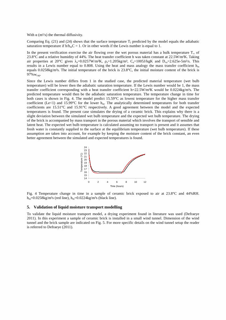
Since the Lewis number differs from 1 in the studied case, the predicted material temperature (wet bulb temperature) will be lower then the adiabatic saturation temperature. If the Lewis number would be 1, the mass transfer coefficient corresponding with a heat transfer coefficient h=22.5W/m²K would be 0.0224kg/m²s. The predicted temperature would then be the adiabatic saturation temperature. The temperature change in time for both cases is shown in Fig. 4. The model predict 15.59°C as lowest temperature for the higher mass transfer coefficient (Le<1) and 15.99°C for the lower hm. The analytically determined temperatures for both transfer coefficients are 15.51°C and 15.91°C respectively. A good agreement between the model and the expected temperatures is found. The present case simulates the drying of a ceramic brick. This explains why there is a slight deviation between the simulated wet bulb temperature and the expected wet bulb temperature. The drying of the brick is accompanied by mass transport in the porous material which involves the transport of sensible and latent heat. The expected wet bulb temperature is calculated assuming no transport is present and it assumes that fresh water is constantly supplied to the surface at the equilibrium temperature (wet bulb temperature). If these assumption are taken into account, for example by keeping the moisture content of the brick constant, an even better agreement between the simulated and expected temperatures is found.

1415161718192021222324

0 2 4 6 8 10 12

Time (hours)

Tem

pera

ture

(°C

)

Fig. 4 Temperature change in time in a sample of ceramic brick exposed to air at 23.8°C and 44%RH. hm=0.0258kg/m²s (red line), hm=0.0224kg/m²s (black line).

5. Validation of liquid moisture transport modelling

To validate the liquid moisture transport model, a drying experiment found in literature was used (Defraeye 2011). In this experiment a sample of ceramic brick is installed in a small wind tunnel. Dimension of the wind tunnel and the brick sample are indicated on Fig. 5. For more specific details on the wind tunnel setup the reader is referred to Defraeye (2011).

Fig. 5 Schematic representation of the experimental setup by Defraeye (2011). The X’s indicate the positions of the thermocouples.

The inlet profile was measured with PIV (particle image velocimetry) and used as input for a CFD model of the wind tunnel. From this CFD model the convective heat transfer coefficient h [W/m²K] was estimated at 22.5W/m²K. Temperatures near the brick sample were monitored at different locations. The sample of ceramic brick was well insulated as indicated on the figure with extruded polystyrene (XPS) and all sides of the brick except one were made impermeable for moisture. The wind tunnel was located inside a climate chamber were the air was preconditioned to 23.8°C and a relative humidity of 44%. Moisture content of the ceramic brick was initially at 97%wcap. The material properties of the test material were already listed in section 4.

For the modelling approach only a cross section of the brick sample is simulated. The insulation on the walls is incorporated into the boundary conditions. Measurements and simulations performed by Defraeye (2011) showed that the heat transfer coefficient on the side walls and bottom he could be estimated at 8W/m²K. The thermal conductivity of the XPS, λXPS, was taken as 0.034W/mK. Side walls and bottom were assumed to be impermeable for moisture. This resulted in the following heat flux boundary condition for the side walls and the bottom:

( )se

XPS

XPS

e

h TTd

h

q −+

=

λ1

1 (27)

Te is the outside temperature (23.8°C) and Ts the temperature at the surface of the brick, dXPS is the insulation thickness (0.02m at the bottom, 0.03m at the sides).

The boundary conditions at the top are given by:

( ) ( ) ( )44

111 sr

sr

bsemseh TT

CYYLhTThq −

−++−+−=

εε

(28)

( )sem YYhg −=r (29)

The second term of Eq. (28) represents the latent heat leaving the computational grid. Here Ye is the mass fraction of water vapour in the surrounding air (corresponding to 44%RH and 23.8°C) and Ys is the mass fraction at the surface. The third term on the right hand side is the heat flux due to radiation. Cb is the Stefan-Boltzmann constant (5.67e10-8kg/s³K4) and εr and εs are respectively the emissivity of the roof and the brick surface (εr=0.97, εs=0.93). The brick is initially at 23.8°C.

The grid used for the simulations had in total 600x20 cells and was very fine near the top surface.

Fig. 6 shows a comparison of the simulation results with the measurements by Defraeye (2011) for the temperature at 10mm. Three cases were simulated using the 2D cross section model of the brick. The three cases differ in the boundary conditions that were used. Case 1 has adiabatic and impermeable walls, except at the top. In case 2 and 3 a heat flux is added at the side and bottom walls according to Eq. 27. For case 2 the conductivity of the insulation λXPS was assumed 0.034W/m²K. In case 3 a failure of the insulation was introduces by increasing the conductivity value to 0.17W/m²K.

1516171819202122232425

0 2 4 6 8 10 12

Time (hours)

Te

mpe

ratu

re (

°C)

Fig. 6 Comparison of measurements performed by Defraeye (2011) (black line) and three simulation cases. Adiabatic boundary conditions (blue line). Case 2 (red line). Case 3 (green line).

Al cases show the correct trends expected during drying. This is also shown in Fig. 7 where the drying rate is plotted in function of time. Initially the drying rate is high since the vapour mass fraction at the surface is high resulting in a maximum driving potential for vapour transport. Due to the water vapour evaporating from the surface, the temperature at the surface starts to drop. This temperature drop results in a decrease of the saturation vapour mass fraction at the surface and consequently a drop of the drying rate. An equilibrium temperature is reached at the surface when the heat leaving the porous material due to evaporation equals the heat added due to convection and conduction. This period with constant temperature is often referred to as the constant drying rate period (CRP). Finally, when the surface of the material start to dry out, the drying rate starts to drop and the temperature at the surface starts to rise again (falling rate period (FRP)). When dryout occurs at the surface the transport of water to the surface is dominated by diffusion of water vapour. This is a slow process which limits the amount of water supplied to the surface and thus limits the drying rate. An imbalance between the heat leaving the surface through evaporation and the heat added due to convection, explains the temperature rise. Fig. 8 shows the evolution of the moisture content in the ceramic brick along the depth of the sample. This figure clearly shows how the moisture content in the material rapidly decreases until the surface starts to dry out. Once dryout occurs, the moisture content decreases slower and a moisture front develops which slowly moves through the porous material away from the surface. Similar results for ceramic brick were found by Landman 2001.

0

0.00005

0.0001

0.00015

0.0002

0.00025

0 2 4 6 8 10 12

Time (hours)

dryi

ng r

ate

(kg/

m²s

)

Fig. 7 Drying rate (kg/m²s) for three cases: case 1 adiabatic side walls (blue line), case 2 heat flux at side walls (red line), case 3 higher heat flux at side walls due to lower insulation value (green line).

0

20

40

60

80

100

120

140

0 0.005 0.01 0.015 0.02 0.025 0.03

depth (m)

moi

stur

e co

nten

t (kg

/m³)

Fig. 8 Evolution in time of the moisture content in a 3cm thick sample of ceramic brick exposed to convective drying conditions. Each line represents the moisture content every two hours.

Fig.6 shows good agreement but no perfect match was found. A more detailed modelling approach with a 3D model and spatially varying transfer coefficients and a direct coupling with the air side will probably lead to better results. This is however left for future research.

6. Conclusions

In this paper a newly developed coupled HAM-CFD model was discussed. A direct coupling was applied where the heat and moisture transport equations were directly implemented into an existing CFD package. Various verification and validation exercises were performed to assess the accuracy of the model.

This verification and validation can be divided into two groups according to the dominant moisture transport mechanism. In a first group, vapour is the main transported phase through the porous material. This transport mechanism occurs in the hygroscopic region (RH<98%). In a second group also liquid moisture transport occurs. This is for example the case in drying phenomena.

A first verification exercise compared an analytical solution to a vapour diffusion problem with the model outcome. An almost perfect agreement was found. Secondly the vapour transport was validated with wind tunnel and climate chamber measurements. These results were not discussed in detail in this paper, but can be found in the referenced papers. Also here a good agreement between measurements and simulations was found.

Finally the liquid moisture transport was verified and validated. It was found that the model is able to accurately predict the wet bulb temperature during a convective drying case. An attempt was made to validate the dying model with experimental data found in literature. A 2D model was used to simulate drying in a sample of ceramic brick. It was concluded that such a model is able to predict the correct trends but a more detailed model is probably needed in 3D with specially varying transfer coefficients to give a better agreement with the measurements.

Acknowledgements

The results presented in this paper have been obtained within the frame of the research project IWT-SB/81322/VanBelleghem funded by the Flemish Institute for the Promotion and Innovation by Science and Technology in Flanders. Its financial support is gratefully acknowledged.

References

Berger D, Pei DCT. 1973. Drying of hygroscopic capillary porous solids - a theoretical approach, International Journal of Heat and Mass Transfer 16, pp. 293-302.

Carmeliet J, Roels S. 2001. Determination of the Isothermal Moisture Transport Properties of Porous Building Materials, Journal of Thermal Envelope and Building Science 24(3), pp. 183-210.

Chen XD, Lin SXQ, Chen G. 2002. On the ratio of heat to mass transfer coefficient for water evaporation and its impact upon drying modeling, International Journal of Heat and Mass Transfer 45(21), pp. 4369-4372.

Chilton TH, Colburn AP. 1934. Mass Transfer (Absorption) Coefficients Prediction from Data on Heat Transfer and Fluid Friction, Industrial and Engineering Chemistry 26, pp. 1183-1187.

Cranck J. 1975. The mathematics of diffusion, Clarendon press, Oxford, UK.

Defraeye T. 2011. Convective Heat and Mass Transfer at Exterior Building Surfaces, Ph.D. thesis, KULeuven, Leuven, Belgium, 334 pp.

Grunewald J. 1997. Diffusiver und konvektiver Stoff- und Energietransport in kapillarporösen Baustoffen, Ph.D. dissertation, Technischen Universität Dresden, Germany, 220pp.

James C, Simonson CJ, Talukdar P, Roels S. 2010. Numerical and experimental data set for benchmarking hygroscopic buffering models, International Journal of Heat and Mass Transfer53(19-20), pp. 3638-3654.

Janssen H, Blocken B, Carmeliet J. 2007. Conservative modelling of the moisture and heat transfer in building components under atmospheric excitation, International Journal of Heat and Mass Transfer 50(5-6), pp. 1128-1140.

Janssen H. 2011. Thermal diffusion of water vapour in porous materials: fact or fiction? Building and Environment 54, pp. 1548-1562.

Landman KA, Pel L, Kaasschieter EF. 2001. Analytic modelling of drying of porous materials, Mathematical Engineering in Industry 8(2), pp. 89-122.

Milly PCD. 1982. Moisture and heat transport in hysteretic, inhomogeneous porous media: a matrix head-based formulation and a numerical model, Water Resources Research 18(3), pp. 489-498.

Philip JR, de Vries DA. 1957. Moisture movement in porous materials under temperature gradients, Transactions of the American Geophysical Union 38, pp. 222-232.

Steeman H-J, Janssens A, Carmeliet J, De Paepe M. 2009a. Modelling indoor air and hygrothermal wall interaction in building simulation: Comparison between CFD and a well-mixed zonal model, Building and Environment 44(3), pp. 572-583.

Steeman H-J, Van Belleghem M, Janssens A, De Paepe M. 2009b. Coupled simulation of heat and moisture transport in air and porous materials for the assessment of moisture related damage, Building and Environment 44(10), pp. 2176-2184.

Steeman M, Janssens A, Steeman HJ, Van Belleghem M, De Paepe M. 2010. On coupling 1D non-isothermal heat and mass transfer in porous materials with a multizone building energy simulation model, Building and Environment 45(4), pp. 865-877.

Steskens P, Janssen H, Rode C. 2009. Influence of the Convective Surface Transfer Coefficients on the Heat, Air, and Moisture (HAM) Building Performance, Indoor and Built Environment 18(3), pp. 245-256.

Sorensen DN, Nielsen PV. 2003. Quality control of computational fluid dynamics in indoor environments, Indoor Air 13(1), pp.2-17.

Van Belleghem M, Steeman H-J, Steeman M, Janssens A, De Paepe M. 2010. Sensitivity analysis of CFD coupled non-isothermal heat and moisture modelling, Building and Environment 45(11), pp. 2485-2496.

Van Belleghem M, Steeman M, Willockx A, Janssens A, De Paepe M. 2011. Benchmark experiments for moisture transfer modelling in air and porous materials, Building and Environment 46(4), pp. 884-898.

Whitaker S. 1977. Simultaneous heat, mass and momentum transfer in porous media: A theory of drying, Academic Press, New York.