development and validation of small punch testing at nist

NISTIR 8303

Development and Validation of Small Punch Testing at NIST

Enrico Lucon Jake Benzing

Nik Hrabe

This publication is available free of charge from:

https://doi.org/10.6028/NIST.IR.8303

NISTIR 8303

Development and Validation of Small Punch Testing at NIST

Enrico Lucon Jake Benzing

Nik Hrabe Applied Chemicals and Materials Division

Material Measurement Laboratory

This publication is available free of charge from: https://doi.org/10.6028/NIST.IR.8303

April 2020

U.S. Department of Commerce Wilbur L. Ross, Jr., Secretary

National Institute of Standards and Technology

Walter Copan, NIST Director and Undersecretary of Commerce for Standards and Technology

Certain commercial entities, equipment, or materials may be identified in this

document in order to describe an experimental procedure or concept adequately. Such identification is not intended to imply recommendation or endorsement by the National Institute of Standards and Technology, nor is it intended to imply that the entities, materials, or equipment are necessarily the best available for the purpose.

National Institute of Standards and Technology Interagency or Internal Report 8303 Natl. Inst. Stand. Technol. Interag. Intern. Rep. 8303, 55 pages (April 2020)

This publication is available free of charge from: https://doi.org/10.6028/NIST.IR.8303

i

This publication is available free of charge from: https://doi.org/10.6028/N

IST.IR.8303

Abstract

Small Punch (SP) testing is a methodology that uses tiny disks (generally 8 mm in diameter and 0.5 mm thick) to estimate mechanical properties of metallic materials, such as tensile properties, fracture toughness, and ductile-to-brittle transition temperature. Empirical correlations are typically used to infer conventional mechanical properties from characteristic forces and displacements obtained from the SP test record. At NIST in Boulder, Colorado, we recently developed experimental and analytical procedures for running SP tests on various materials. We conducted SP tests on three steels with widely different tensile and fracture properties. The NIST setup was successfully qualified by comparing our results on A533B steel to the results obtained in an international round-robin, and also by comparing empirical correlations between SP data and tensile properties to similar relationships published in the literature. We also tested specimens with different surface roughness, to investigate the influence of surface finish on SP test results. Key words

Empirical correlations; international round-robin; Small Punch; surface roughness; tensile properties.

ii


IST.IR.8303

Table of Contents Introduction ..................................................................................................................... 1 Experimental setup .......................................................................................................... 3 Materials and test conditions .......................................................................................... 4 Measurements of test system compliance ...................................................................... 6 Analysis of an individual SP test .................................................................................... 7 5.1. Elastic-plastic transition force, Fe ............................................................................... 9

5.2. Maximum force, Fm ................................................................................................... 10

5.3. Displacement at end of test, vf ................................................................................... 10

5.4. SP fracture energy, ESP .............................................................................................. 10

5.5. SP total energy, Em .................................................................................................... 11

5.6. SP plastic energy, EPL ................................................................................................ 11

5.7. Effective fracture strain, εf ........................................................................................ 11

5.8. Additional parameters ............................................................................................... 11

Test results...................................................................................................................... 11 6.1. JRQ steel .................................................................................................................... 11

6.1.1. Comparison with round-robin results .................................................................. 12

6.2. Low-energy 4340 steel (4340LL) .............................................................................. 13

6.3. High-energy 4340 steel (4340HH) ............................................................................ 14

Correlations with tensile properties ............................................................................. 15 7.1. Yield strength correlations ........................................................................................ 15

7.2. Tensile strength correlations ..................................................................................... 20

7.3. Total elongation correlations ..................................................................................... 24

Additional correlations (not previously published) .................................................... 26 8.1. Uniform elongation ................................................................................................... 26

8.2. Charpy absorbed energy ............................................................................................ 26

Discussion: effect of specimen surface finish .............................................................. 27 Conclusions .................................................................................................................... 28

References .............................................................................................................................. 28 List of Tables Table 1 - Chemical composition of the JRQ and 4340 steels (wt %). ...................................... 5 Table 2 – Tensile properties of the JRQ and 4340 steels. ......................................................... 5 Table 3 - Results of compliance measurements. ....................................................................... 6 Table 4 - Results of SP tests on JRQ steel (rough specimens). .............................................. 12 Table 5 - Results of SP tests on JRQ steel (polished specimens). .......................................... 12 Table 6 - Comparison between round-robin (R-R) and NIST force results for the JRQ steel.................................................................................................................................................. 12

iii


IST.IR.8303

Table 7 - Results of SP tests on 4340LL steel (rough specimens). ......................................... 13 Table 8 - Results of SP tests on 4340LL steel (polished specimens). .................................... 14 Table 9 - Results of SP tests on 4340HH steel (rough specimens). ........................................ 14 Table 10 - Results of SP tests on 4340HH steel (polished specimens). ................................. 14 Table 11 - Influence of specimen surface finish on SP test results: results of two-sample t-tests on means of characteristic parameters. ......................................................................... 27 List of Figures Figure 1 - Schematic representation of the SP test method. ..................................................... 1 Figure 2 - Typical form of a SP force-deflection diagram for steel, showing five distinct regions [1]. ................................................................................................................................ 2 Figure 3 - SP testing fixture used at NIST, shown disassembled (left) and assembled (right). 3 Figure 4 - SP testing fixture mounted on the test machine with the extensometer for punch displacement measurement. ...................................................................................................... 3 Figure 5 – Cross-sectional view of SP test setup [14]. The LVDT measuring specimen deflection (u) is indicated as item 5. Punch displacement is indicated as v. ............................. 4 Figure 6 - Dimensions and tolerances of SP specimens [11]. ................................................... 5 Figure 7 - Compliance measurements as a function of actuator displacement. ........................ 7 Figure 8 - Compliance measurements as a function of extensometer displacement. ............... 7 Figure 9 - Force-displacement curves for an SP test on JRQ steel. .......................................... 8 Figure 10 - Force-displacement curves for an SP test on 4340LL steel. .................................. 8 Figure 11 - Force-displacement curves for an SP test on 4340HH steel. ................................. 9 Figure 12 - Determination of the elastic-plastic transition force, Fe. ..................................... 10 Figure 13 - Comparison between mean force values reported by round-robin participants and NIST on the JRQ steel. Error bands correspond to ± twice the standard deviation. .............. 13 Figure 14 - Correlations between yield strength and SP elastic-plastic transition force. The purple dashed line is the linear fit to the rough specimen data, while the pink dash-dotted line is the linear fit to the polished specimen data. ........................................................................ 16 Figure 15 - Comparison between NIST results and the correlation in [24]. ........................... 18 Figure 16 - Comparison between NIST results and the correlation in [19]. ........................... 18 Figure 17 - Comparison between NIST results and the correlation in [19]. ........................... 19 Figure 18 - Comparison between NIST results and the correlation in [18,20]. ...................... 19 Figure 19 - Comparison between NIST results and the correlation in [23]. ........................... 19 Figure 20 - Comparison between NIST results and the correlation in [23]. ........................... 20 Figure 21 - Comparison between NIST results and the correlation in [30]. ........................... 20 Figure 22 - Correlations between tensile strength and SP maximum force, normalized by ℎ02. The purple dashed line is the linear fit to the rough specimen data, while the pink dash-dotted line is the linear fit to the polished specimen data. ................................................................. 21 Figure 23 - Correlations between tensile strength and SP maximum force, normalized by 𝑢𝑢𝑚𝑚ℎ0. ...................................................................................................................................... 22

iv


IST.IR.8303

Figure 24 - Comparison between NIST results and the correlation in [23]. ........................... 23 Figure 25 - Comparison between NIST results and the correlation in [25]. ........................... 23 Figure 26 - Comparison between NIST results and the correlations in [23,26]. .................... 23 Figure 27 - Comparison between NIST results and the correlation in [33]. ........................... 24

Figure 28 - Comparison between NIST results and the correlations in [19,27] for εt. ........... 25

Figure 29 - Comparison between NIST results and the correlations in [19,28] for εt. ........... 25

Figure 30 - Comparison between NIST results and the correlation in [29] for εt. .................. 25 Figure 31 - Correlations between uniform elongation and 𝑢𝑢𝑚𝑚ℎ0 obtained at NIST. ............. 26 Figure 32 - Correlations between Charpy absorbed energy and SP energies for rough and polished specimens. ................................................................................................................ 27 List of Annexes Annex 1 – Operational Procedure for Performing Small Punch tests at NIST in Boulder,

Colorado Annex 2 – Spreadsheet-Based Software for the Analysis of a Small Punch Test Annex 3 – Summary of Correlations between SP Parameters and Tensile Properties (from the

literature, 1998-2019, and obtained at NIST)

v


IST.IR.8303

Glossary

ASTM American Society for Testing and Materials CEN European Committee for Standardization EDM Electro-Discharge Machining D In SP testing, specimen diameter (mm) dv/dt In SP testing, punch displacement rate (mm/s) Em In SP testing, total energy calculated up to um (J) EPL In SP testing, plastic energy calculated up to um (J) ESP In SP testing, fracture energy calculated up to uf (J) εf In SP testing, effective fracture strain 𝜀𝜀�̇�𝑆𝑆𝑆𝑚𝑚𝑚𝑚𝑚𝑚 In SP testing, estimated maximum strain rate (1/s) εt In tensile testing, total elongation (%) εu In tensile testing, uniform elongation (%) F Force (N) Fe In SP testing, elastic-plastic transition force (N) Fept In SP testing, force at the point of maximum curvature (N) Fe1.5 In SP testing, force corresponding to the point where the ratio between area under

the curve and above the curve equals 1.5 (N) Fh0/10,off In SP testing, force at the intersection between the test record and a line parallel to

the slope of the initial linear region with an offset of 0.1∙h0 (N) Finfl In SP testing, force at the inflection point of the curve (d2F/du2 = 0) (N) Fm In SP testing, maximum force (N) F0.1mm,off In SP testing, force at the intersection between the test record and a line parallel to

the slope of the initial linear region with an offset of 0.1 mm (N) F0.1mm In SP testing, force corresponding to a displacement value of 0.1 mm (N) F0.48mm In SP testing, force corresponding to a displacement value of 0.48 mm (N) F0.5mm In SP testing, force corresponding to a displacement value of 0.5 mm (N) F0.645mm In SP testing, force corresponding to a displacement value of 0.645 mm (N) F0.65mm In SP testing, force corresponding to a displacement value of 0.65 mm (N) F0.9mm In SP testing, force corresponding to a displacement value of 0.9 mm (N) f(v) In SP testing, bilinear function used to determine Fe [10,11]. h0 In SP testing, initial specimen thickness (mm) ISO International Standardization Organization K In SP testing, curvature parameter according to [30] KV Charpy absorbed energy (J) r Pearson correlation coefficient Ra Surface roughness (µm) Rm In tensile testing, tensile strength (MPa)

vi


IST.IR.8303

Rp02 In tensile testing, yield strength (MPa) Slopeini In SP testing, slope of the initial elastic region of the curve (N/mm) SP Small Punch tcalc Calculated value of the t-test statistic tcritical Critical value of the t-test statistic (if tcalc > tcritical, means are statistically different) u Specimen deflection (mm) v Punch displacement (mm) vf In SP testing, punch displacement corresponding to a 20 % force drop with respect

to maximum force (mm) vm In SP testing, punch displacement at maximum force (mm) v1p In SP testing, punch displacement at the occurrence of the first significant pop-in

(mm).

1


IST.IR.8303

Introduction

In the field of experimental techniques based on sub-size or miniaturized specimens, methodologies based on testing tiny disks represent a method for characterizing the mechanical properties of service-exposed plant components or structures with a minimal amount of material extracted from the component and subjected to destructive testing [1]. Moreover, a significant number of disk specimens can be extracted from machining leftovers or already tested conventional specimens.

The Small Punch (SP) test, also known as the Disk Bend test, was developed in the mid-1980s [2,3] through the use of tiny disks of 3 mm diameter and 0.25 mm thickness, centrally loaded by a spherical ball or hemispherical punch, and expanded into a larger lower die. The test system was a module that could be placed between the loading platens of a tensile machine and subsequently loaded [3]. The outcome is a bulge in the disk rather than a shear cut, as in a similar methodology called the Shear Punch test [4]. Although disks of these dimensions are still used for SP testing, nowadays the most popular specimen geometry (which is used in this investigation) is a round disk with a diameter of 8 mm and a thickness of 0.5 mm, which is the geometry used in this study. The use of square specimens (10 mm × 10 mm) has also been reported [5].

A schematic representation of the SP test method is shown in Fig. 1.

Figure 1 - Schematic representation of the SP test method.

The general form of a SP force/deflection test record for a steel specimen is shown in Fig. 2 [1]. Five distinct regions can be identified: 1. Elastic region, 2. Departure from linearity (elastic-plastic transition), 3. Local bending, transitioning to a membrane stress regime, 4. Membrane stress regime, and 5. Final failure region.

The general form of the test record suggests that yield stress may be associated with the change in slope between regions 1 and 2, while the ultimate tensile stress may be related to the maximum force, and ductility to maximum deflection. Note that, for steels showing low ductility, regions 4 and 5 may be virtually absent or minimized.

2


IST.IR.8303

Figure 2 - Typical form of a SP force-deflection diagram for steel, showing five distinct

regions [1]. Characteristic values of force, displacement, and energy (calculated by integrating

force and displacement) are identified on the test record. These values are generally fed into empirical relations to obtain estimates of specific mechanical parameters (tensile properties, ductile-to-brittle transition temperature, fracture toughness) for the material under investigation. Numerous empirical correlations are available in the literature, and have been developed by comparing characteristic parameters from SP tests with tensile properties, transition temperature data, and fracture toughness values measured by means of conventional tests.

In most cases, correlations appear to be strongly dependent on the material (or the class of material) under investigation, and cannot be expected to be applicable to other materials or material conditions [5].

Note that alternative approaches, of a more analytical nature, have also been proposed. Several authors have matched force-displacement curves from SP tests, up to the point of observed crack initiation, to a database of curves corresponding to a range of stress-strain constitutive behaviors. The model used in this case is a Ramberg-Osgood model with a possible modification to accommodate the discontinuous yield observed in several low-alloy steels [6]. Other analytical methods have also been proposed, involving the use of Neural Networks and Finite Element simulations [7-9].

The approach used in this report for the analysis of SP test results, however, is strictly of a correlative nature.

Even though researchers all over the world have been performing SP tests since the 1980s, an official test standard issued by an internationally recognized standardization body (ASTM or ISO), is still missing.

The available document that most closely resembles a Test Standard is a European CEN1 Workshop Agreement, CWA 15627 (Small Punch Test Method for Metallic Materials), issued in 2007 [10]. At the time of writing, a Draft ASTM Test Method for Small Punch Testing of Metallic Materials [11], modeled after CWA 15627, is being developed inside the ASTM E10.02 Sub-Committee (Behavior and Use of Nuclear Materials).

1 CEN: Comité Européen de Normalisation (European Committee for Standardization).

3


IST.IR.8303

Experimental setup

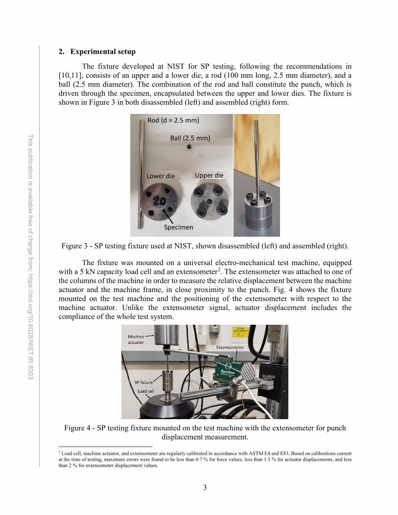
The fixture developed at NIST for SP testing, following the recommendations in [10,11], consists of an upper and a lower die, a rod (100 mm long, 2.5 mm diameter), and a ball (2.5 mm diameter). The combination of the rod and ball constitute the punch, which is driven through the specimen, encapsulated between the upper and lower dies. The fixture is shown in Figure 3 in both disassembled (left) and assembled (right) form.

Figure 3 - SP testing fixture used at NIST, shown disassembled (left) and assembled (right).

The fixture was mounted on a universal electro-mechanical test machine, equipped with a 5 kN capacity load cell and an extensometer2. The extensometer was attached to one of the columns of the machine in order to measure the relative displacement between the machine actuator and the machine frame, in close proximity to the punch. Fig. 4 shows the fixture mounted on the test machine and the positioning of the extensometer with respect to the machine actuator. Unlike the extensometer signal, actuator displacement includes the compliance of the whole test system.

Figure 4 - SP testing fixture mounted on the test machine with the extensometer for punch

displacement measurement.

2 Load cell, machine actuator, and extensometer are regularly calibrated in accordance with ASTM E4 and E83. Based on calibrations current at the time of testing, maximum errors were found to be less than 0.7 % for force values, less than 1.5 % for actuator displacements, and less than 2 % for extensometer displacement values.

4


IST.IR.8303

The operational procedure for conducting an SP test at NIST in Boulder is detailed in Annex 1.

Many researchers have also reported direct measurements of specimen deflection by the use of a Linear Voltage Displacement Transducer (LVDT) that monitors the displacement of a point at the center of the specimen opposite to the punch (Fig. 5).

Figure 5 – Cross-sectional view of SP test setup [14]. The LVDT measuring specimen

deflection (u) is indicated as item 5. Punch displacement is indicated as v.

Currently, the test rig developed at NIST does not accommodate for deflection measurement below the specimen, and therefore all analyses in this study were performed on the basis of punch displacement (v), corrected for test system compliance. It is possible that in the future we will develop a modified fixture that also allows measuring specimen deflection.

Materials and test conditions

For the validation of the experimental and analytical procedures used at NIST for SP testing, we selected three steels for which conventionally measured tensile properties were available:

• A533B Cl. 1 reactor pressure vessel (RPV) steel, with denomination JRQ. This is a reference RPV steel, widely used in the nuclear community as a radiation/mechanical property correlation monitor material in a number of international and national studies of irradiation embrittlement [12]. This JRQ steel is one of the materials used in an Interlaboratory Study (round-robin) conducted in 2017 to qualify the ASTM Test Method [11,13]. This allowed us to directly compare our results with those reported by round-robin participants.

• 4340 steel, used by NIST to produce low-energy certified reference Charpy specimens3, heat treated to attain impact energies in the range 15-20 J at room temperature [14]. We will herein identify this steel as 4340LL.

• 4340 steel, used by NIST to produce high-energy certified reference Charpy specimens2, heat treated to attain impact energies in the range 100-120 J at room temperature [14]. We will herein identify this steel as 4340HH.

3 In accordance with ASTM E23 and ISO 148-2.

5


IST.IR.8303

The chemical composition and the tensile properties of the steels are provided in Table 1 and Table 2. As shown in Table 2, the selected steels cover a wide range of strength and ductility.

Table 1 - Chemical composition of the JRQ and 4340 steels (%, mass fraction). Steel C Si Mn P S Mo Ni Cr Cu Ref. JRQ 0.07 0.21 1.34 0.02 0.002 0.49 0.70 0.11 0.15 [12]

4340LL 0.40 0.28 0.66 0.004 0.001 0.28 1.77 0.83 N/A [14] 4340HH

Table 2 – Tensile properties of the JRQ and 4340 steels.

Steel Rp02 (MPa)

Rm (MPa)

εu (%)

εt (%) Ref.

JRQ 477 630 13.0 26.0 [12] 4340LL 1354 1513 3.4 10.9 [15] 4340HH 928 1060 7.1 19.6

All SP tests were performed at room temperature (21 °C ± 2 °C) in actuator displacement control, with a speed of approximately 0.015 mm/s. The ASTM Draft Test Method allows displacement rates between 0.0033 mm/s and 0.033 mm/s, with 0.0083 mm/s (0.5 mm/min) as the most commonly used value. According to [10,11], the following formula provides a reasonable estimate of the maximum punch strain rate, 𝜀𝜀�̇�𝑆𝑆𝑆𝑚𝑚𝑚𝑚𝑚𝑚, as a function of the punch displacement rate dv/dt:

𝜀𝜀�̇�𝑆𝑆𝑆𝑚𝑚𝑚𝑚𝑚𝑚 ≈ 1000 m−1 ∙ 𝑑𝑑𝑑𝑑𝑑𝑑𝑑𝑑

(1)

Force, actuator displacement, and punch displacement (extensometer) data were recorded at a sampling frequency of 1 Hz. The compliance of the test system was measured as detailed in Sec. 4, and subtracted from both actuator and extensometer displacements in order to obtain actual punch displacement values, v.

Data analysis was conducted in accordance with [11] by means of a spreadsheet-based software developed in-house. The software and its use are described in detail in Annex 2.

SP specimens were machined out of Charpy specimens (both untested and tested) by means of Electrical Discharge Machining (EDM), in accordance with the dimensions and tolerances shown in Fig. 6 [11].

Figure 6 - Dimensions and tolerances of SP specimens [11].

In this investigation, the influence of surface finish was studied by examining two specimen conditions:

• “rough” (as-received) specimens, with surface roughness, Ra, in the range from 3 µm to 4 µm, resulting from the EDM process;

6


IST.IR.8303

• “polished” specimens, with surface roughness, Ra, in the range from 0.1 µm to 0.25 µm. This surface condition was obtained by manually grinding slightly oversized as-machined specimens (thickness ≈ 0.55 mm) on abrasive paper with a grit size of P400, followed by fine grinding (P1200) down to the final thickness. Both [10] and [11] require Ra < 0.25 µm. Before testing, the following measurements were performed and reported for each

specimen: • diameter D, measured with a digital comparator; • thickness h0, measured with a caliper; • surface roughness Ra, measured with a portable surface roughness tester.

Measurements of test system compliance

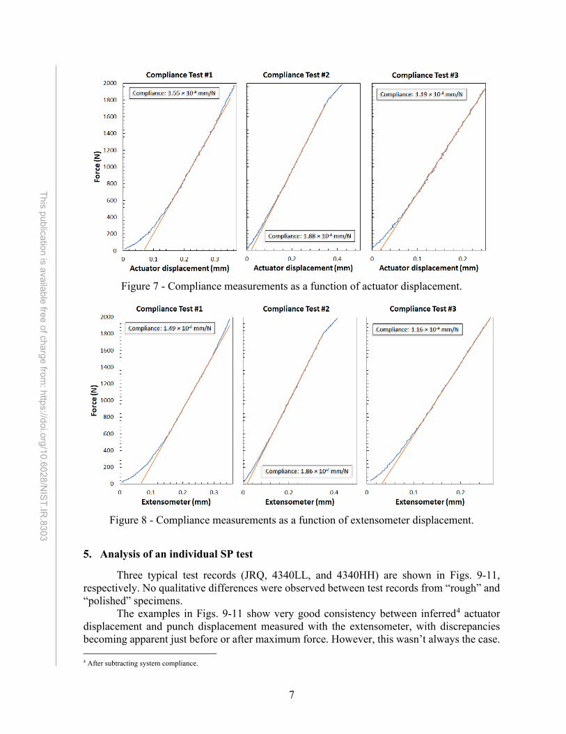
For measuring system compliance, we performed three tests without a specimen in place. The rod + ball system was pressed against the lower plate of the test machine up to the first deviation from linearity (around 1,800 N), to avoid permanent deformation of the rod. Force, actuator displacement, and extensometer signal were recorded with the same sampling frequency of the SP test (1 Hz).

System compliance was calculated as the inverse of the slope of the linear part of the test record, approximately between 600 N and 1,400 N (Figs. 7 and 8). The linear regressions were performed by means of the SDAR (Slope Determination by the Analysis of Residuals) algorithm [16]. The regression coefficients for the three tests, and the resulting system compliances in terms of actuator displacements and extensometer displacements, are given in Table 3.

System compliances were quite similar between actuator and extensometer, with the former predictably higher. Force-actuator displacement and force-extensometer signal curves are shown in Fig. 7 and Fig. 8, respectively, with corresponding linear regressions.

The average compliance values used in the SP test analyses and subtracted from the recorded actuator and extensometer displacements, as a function of applied force, were: 1.54 × 10-4 mm/N (actuator) and 1.50 × 10-4 (extensometer).

Table 3 - Results of compliance measurements.

Test # Actuator Extensometer

Slope (N/mm)

Intercept (N)

Compliance (mm/N)

Slope (N/mm)

Intercept (N)

Compliance (mm/N)

1 6453.47 -437.84 1.55×10-4 6699.42 -445.19 1.49×10-4 2 5331.16 -103.82 1.88×10-4 5378.17 -86.96 1.86×10-4 3 8370.66 -151.69 1.19×10-4 8614.41 -273.91 1.16×10-4

Average 6718.43 -231.11 1.54×10-4 6897.33 -268.69 1.50×10-4 St. dev. 23 % 78 % 22 % 24 % 67 % 23 %

7


IST.IR.8303

Figure 7 - Compliance measurements as a function of actuator displacement.

Figure 8 - Compliance measurements as a function of extensometer displacement.

Analysis of an individual SP test

Three typical test records (JRQ, 4340LL, and 4340HH) are shown in Figs. 9-11, respectively. No qualitative differences were observed between test records from “rough” and “polished” specimens.

The examples in Figs. 9-11 show very good consistency between inferred4 actuator displacement and punch displacement measured with the extensometer, with discrepancies becoming apparent just before or after maximum force. However, this wasn’t always the case.

4 After subtracting system compliance.

8


IST.IR.8303

For some tests, the two signals started diverging just after the beginning of the test. This was most likely caused by the slightly different positioning of the extensometer arm on the upper machine actuator from test to test. Such tests were included in the overall data analyses.

In this investigation, we used inferred extensometer signal (blue curves in Figs. 9-11) for calculating the results and establishing the correlations with tensile properties.

Figure 9 - Force-displacement curves for an SP test on JRQ steel.

Figure 10 - Force-displacement curves for an SP test on 4340LL steel.

0

200

400

600

800

1000

1200

1400

1600

1800

2000

0 0.5 1 1.5 2 2.5

Forc

e (N

)

Displacement (mm)

Actuator displacementPunch displacement

Punch displacement rate = 0.0015 mm/s

um

Fm

Fe

Ff

uf

0

500

1000

1500

2000

0 0.25 0.5 0.75 1 1.25 1.5

Forc

e (N

)

Displacement (mm)



um

Fm

Fe

Ff

uf

9


IST.IR.8303

Figure 11 - Force-displacement curves for an SP test on 4340HH steel.

In according with [10,11], the following characteristic values are determined from F-u or F-v curves. 5.1. Elastic-plastic transition force, Fe

Fe is defined as the force characterizing the transition from linearity to the stage associated with the spread of the yield zone through the specimen thickness (plastic bending stage) [10,11].

It is determined through the establishment of a bilinear function f(v) from the origin through the points A and B, defined as (Fig. 12):

𝑓𝑓(𝑣𝑣) = �

𝑓𝑓𝐴𝐴𝑢𝑢𝐴𝐴𝑣𝑣 for 0 ≤ 𝑣𝑣 < 𝑣𝑣𝐴𝐴

𝑓𝑓𝐵𝐵−𝑓𝑓𝐴𝐴𝑢𝑢𝐵𝐵−𝑢𝑢𝐴𝐴

(𝑣𝑣 − 𝑣𝑣𝐴𝐴) + 𝑓𝑓𝐴𝐴 for 𝑣𝑣𝐴𝐴 ≤ 𝑣𝑣 ≤ 𝑣𝑣𝐵𝐵 . (2)

The variables fA, fB, and vA are obtained by minimizing the error:

𝑒𝑒𝑒𝑒𝑒𝑒 = ∫ [𝐹𝐹(𝑣𝑣) − 𝑓𝑓(𝑣𝑣)]2𝑑𝑑𝑣𝑣𝑑𝑑𝐵𝐵0 (3)

In Eqs. (2) and (3), vB is taken as the original thickness of the specimen, i.e., vB = h0 = 0.5 mm. The corresponding yield displacement is ve = vA, while the experimental transition force Fe is obtained from the experimental test record as Fe = F(vA), see Fig. 12.

0

500

1000

1500

2000

0 0.2 0.4 0.6 0.8 1 1.2 1.4 1.6 1.8

Forc

e (N

)

Displacement (mm)



um

Fm

Fe

Ff

uf

POP-IN

10


IST.IR.8303

Figure 12 - Determination of the elastic-plastic transition force, Fe.

5.2. Maximum force, Fm

Fm is defined as the maximum force recorded during the SP test [10,11]. It is indicated by a red circle in Figs. 9-11. The corresponding value of punch displacement is vm.

5.3. Displacement at end of test, vf

The end of an SP test is defined by a 20 % force decrease with respect to Fm [10,11]. The corresponding punch displacement is vf.

If the specimen exhibits sudden force drops (pop-ins), caused by unstable crack propagation events followed by crack arrests, vf is replaced by v1p, the displacement corresponding to the first significant pop-in5.

For the SP tests documented in this report, significant pop-ins were observed at maximum force for most 4340LL specimens (example in Fig. 10) and after maximum force for most 4340HH specimens (example in Fig. 11).

5.4. SP fracture energy, ESP

The SP fracture energy is calculated as the area under the force-displacement curve up to vf or v1p [10,11]:

𝐸𝐸𝑆𝑆𝑆𝑆 = ∫ 𝐹𝐹(𝑣𝑣)𝑑𝑑𝑣𝑣𝑑𝑑𝑓𝑓0 . (4)

5 A pop-in is considered significant if it is associated to a force drop of at least 10 %.

0

100

200

300

400

500

600

0 0.05 0.1 0.15 0.2 0.25 0.3 0.35 0.4

Forc

e (N

)

Punch displacement (mm)ve = vA

fAFe A

B

11


IST.IR.8303

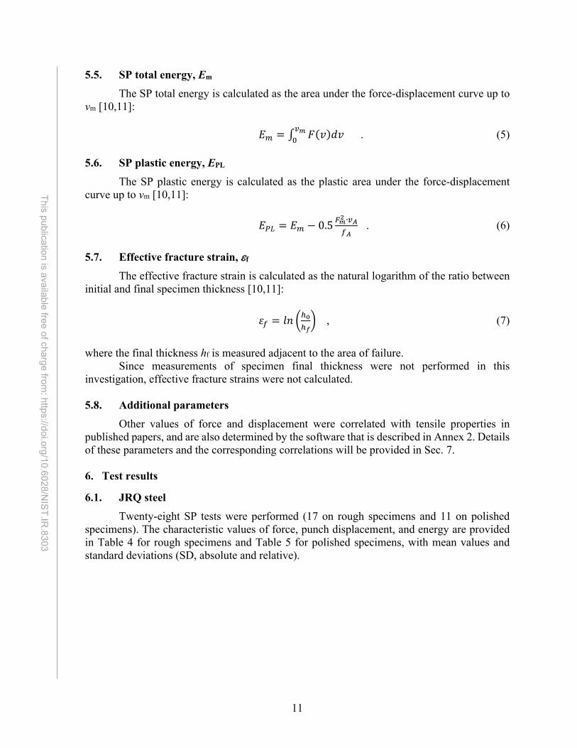
5.5. SP total energy, Em The SP total energy is calculated as the area under the force-displacement curve up to

vm [10,11]:

𝐸𝐸𝑚𝑚 = ∫ 𝐹𝐹(𝑣𝑣)𝑑𝑑𝑣𝑣𝑑𝑑𝑚𝑚0 . (5)

5.6. SP plastic energy, EPL

The SP plastic energy is calculated as the plastic area under the force-displacement curve up to vm [10,11]:

𝐸𝐸𝑆𝑆𝑃𝑃 = 𝐸𝐸𝑚𝑚 − 0.5 𝐹𝐹𝑚𝑚2 ∙𝑑𝑑𝐴𝐴𝑓𝑓𝐴𝐴

. (6)

5.7. Effective fracture strain, εf

The effective fracture strain is calculated as the natural logarithm of the ratio between initial and final specimen thickness [10,11]:

𝜀𝜀𝑓𝑓 = 𝑙𝑙𝑙𝑙 �ℎ0ℎ𝑓𝑓� , (7)

where the final thickness hf is measured adjacent to the area of failure. Since measurements of specimen final thickness were not performed in this investigation, effective fracture strains were not calculated. 5.8. Additional parameters

Other values of force and displacement were correlated with tensile properties in published papers, and are also determined by the software that is described in Annex 2. Details of these parameters and the corresponding correlations will be provided in Sec. 7.

Test results

6.1. JRQ steel Twenty-eight SP tests were performed (17 on rough specimens and 11 on polished

specimens). The characteristic values of force, punch displacement, and energy are provided in Table 4 for rough specimens and Table 5 for polished specimens, with mean values and standard deviations (SD, absolute and relative).

12


IST.IR.8303

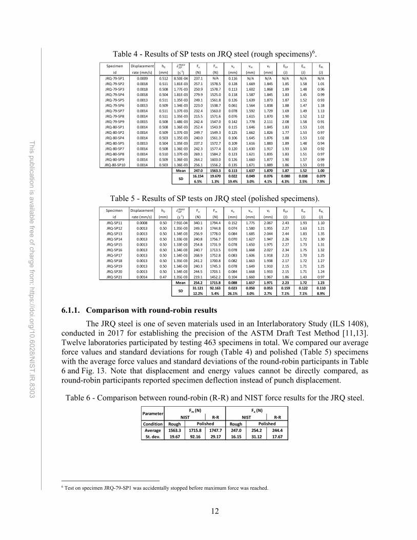
Table 4 - Results of SP tests on JRQ steel (rough specimens)6.

Table 5 - Results of SP tests on JRQ steel (polished specimens).

6.1.1. Comparison with round-robin results The JRQ steel is one of seven materials used in an Interlaboratory Study (ILS 1408),

conducted in 2017 for establishing the precision of the ASTM Draft Test Method [11,13]. Twelve laboratories participated by testing 463 specimens in total. We compared our average force values and standard deviations for rough (Table 4) and polished (Table 5) specimens with the average force values and standard deviations of the round-robin participants in Table 6 and Fig. 13. Note that displacement and energy values cannot be directly compared, as round-robin participants reported specimen deflection instead of punch displacement.

Table 6 - Comparison between round-robin (R-R) and NIST force results for the JRQ steel.

6 Test on specimen JRQ-79-SP1 was accidentally stopped before maximum force was reached.

Specimen Displacement h0 Fe Fm ve vm vf ESP Em EPL

id rate (mm/s) (mm) (s-1) (N) (N) (mm) (mm) (mm) (J) (J) (J)JRQ-79-SP1 0.0009 0.512 8.50E-04 237.1 0.116 N/A N/A N/A N/A N/AJRQ-79-SP2 0.0018 0.511 1.81E-03 257.1 1578.5 0.128 1.669 1.845 1.85 1.58 1.01JRQ-79-SP3 0.0018 0.508 1.77E-03 250.9 1578.7 0.113 1.602 1.868 1.89 1.48 0.96JRQ-79-SP4 0.0018 0.504 1.81E-03 279.9 1525.0 0.118 1.587 1.845 1.83 1.45 0.99JRQ-79-SP5 0.0013 0.511 1.35E-03 249.1 1561.8 0.126 1.639 1.873 1.87 1.52 0.93JRQ-79-SP6 0.0013 0.509 1.34E-03 223.0 1538.7 0.061 1.564 1.838 1.88 1.47 1.18JRQ-79-SP7 0.0014 0.511 1.37E-03 232.4 1563.0 0.078 1.592 1.729 1.69 1.49 1.13JRQ-79-SP8 0.0014 0.511 1.35E-03 215.5 1571.6 0.076 1.615 1.870 1.90 1.52 1.12JRQ-79-SP9 0.0015 0.508 1.48E-03 242.4 1547.0 0.142 1.778 2.111 2.08 1.58 0.91JRQ-80-SP1 0.0014 0.508 1.36E-03 252.4 1543.9 0.115 1.646 1.845 1.83 1.53 1.01JRQ-80-SP2 0.0014 0.509 1.37E-03 249.7 1549.3 0.125 1.662 1.826 1.77 1.53 0.97JRQ-80-SP4 0.0014 0.503 1.35E-03 240.0 1561.3 0.106 1.645 1.876 1.88 1.53 1.02JRQ-80-SP5 0.0013 0.504 1.35E-03 237.2 1572.7 0.109 1.616 1.883 1.89 1.48 0.94JRQ-80-SP7 0.0014 0.508 1.36E-03 242.3 1577.4 0.120 1.630 1.917 1.93 1.50 0.92JRQ-80-SP8 0.0014 0.510 1.37E-03 269.1 1584.2 0.123 1.621 1.835 1.83 1.51 0.97JRQ-80-SP9 0.0014 0.509 1.36E-03 264.2 1603.0 0.126 1.660 1.877 1.90 1.57 0.99JRQ-80-SP10 0.0014 0.503 1.36E-03 256.1 1556.2 0.135 1.671 1.889 1.86 1.53 0.93

Mean 247.0 1563.3 0.113 1.637 1.870 1.87 1.52 1.0016.154 19.670 0.022 0.049 0.076 0.080 0.038 0.0796.5% 1.3% 19.4% 3.0% 4.1% 4.3% 2.5% 7.9%

SD

N/A

𝜀𝜀̇𝑆𝑆𝑆𝑆𝑚𝑚𝑚𝑚𝑚𝑚


id rate (mm/s) (mm) (s-1) (N) (N) (mm) (mm) (mm) (J) (J) (J)JRQ-SP11 0.0008 0.50 7.91E-04 340.1 1794.4 0.152 1.775 2.067 2.43 1.93 1.10JRQ-SP12 0.0013 0.50 1.35E-03 249.3 1744.8 0.074 1.580 1.955 2.27 1.63 1.21JRQ-SP13 0.0013 0.50 1.34E-03 256.9 1778.0 0.084 1.685 2.044 2.44 1.83 1.35JRQ-SP14 0.0013 0.50 1.33E-03 240.8 1756.7 0.070 1.627 1.947 2.26 1.72 1.30JRQ-SP15 0.0013 0.50 1.33E-03 254.8 1731.9 0.078 1.650 1.975 2.27 1.73 1.31JRQ-SP16 0.0013 0.50 1.34E-03 240.7 1713.5 0.078 1.668 2.027 2.34 1.75 1.32JRQ-SP17 0.0013 0.50 1.34E-03 268.9 1752.8 0.083 1.606 1.918 2.23 1.70 1.25JRQ-SP18 0.0013 0.50 1.35E-03 241.2 1700.8 0.082 1.663 1.938 2.17 1.72 1.27JRQ-SP19 0.0013 0.50 1.34E-03 240.3 1745.3 0.078 1.649 1.910 2.15 1.71 1.25JRQ-SP20 0.0013 0.50 1.34E-03 244.5 1703.1 0.084 1.668 1.933 2.15 1.71 1.24JRQ-SP21 0.0014 0.47 1.35E-03 219.1 1452.2 0.104 1.660 1.967 1.86 1.43 0.97

Mean 254.2 1715.8 0.088 1.657 1.971 2.23 1.72 1.2331.121 92.163 0.023 0.050 0.053 0.159 0.122 0.11012.2% 5.4% 26.1% 3.0% 2.7% 7.1% 7.1% 8.9%

SD


R-R R-RCondition Rough RoughAverage 1563.3 1715.8 1747.7 247.0 254.2 244.4St. dev. 19.67 92.16 29.17 16.15 31.12 17.67

PolishedNIST

Polished

ParameterFm (N) Fe (N)

NIST

13


IST.IR.8303

Our force results on polished specimens are in excellent agreement with the round-robin results7, with ±2σ error bands largely overlapping. Results from rough specimens are also statistically not different, except for maximum force values (Fig. 13).

Figure 13 - Comparison between mean force values reported by round-robin participants and

NIST on the JRQ steel. Error bands correspond to ± twice the standard deviation.

6.2. Low-energy 4340 steel (4340LL) Nineteen SP tests were performed (10 on rough specimens and 9 on polished

specimens). The characteristic values of force, punch displacement, and energy are provided in Table 7 for rough specimens and Table 8 for polished specimens, with mean values and standard deviations (absolute and relative).

Table 7 - Results of SP tests on 4340LL steel (rough specimens).

7 Specimens tested in the round-robin were also polished to Ra < 0.25 mm, in accordance with the ASTM Draft Test Method [11].

0

200

400

600

800

1000

1200

1400

1600

1800

2000

Forc

e (N

)NIST (rough)NIST (polished)Round-Robin

FeFm


id rate (mm/s) (mm) (s-1) (N) (N) (mm) (mm) (mm) (J) (J) (J)LL-SP1 0.0010 0.503 9.58E-04 684.5 1893.4 0.180 0.898 1.075 1.40 1.10 0.64LL-SP2 0.0009 0.505 9.23E-04 722.6 1886.4 0.173 0.907 1.099 1.45 1.13 0.71LL-SP3 0.0009 0.505 9.45E-04 651.6 1840.1 0.160 0.851 1.025 1.29 1.02 0.62LL-SP4 0.0009 0.506 9.28E-04 649.3 1897.2 0.130 0.878 1.122 1.52 1.13 0.79LL-SP5 0.0009 0.503 9.31E-04 654.3 1880.7 0.139 0.792 0.951 1.22 0.96 0.60LL-SP6 0.0009 0.506 9.41E-04 672.9 1860.1 0.123 0.823 1.053 1.41 1.04 0.74LL-SP7 0.0009 0.505 9.27E-04 640.1 1958.3 0.136 0.861 1.086 1.48 1.10 0.71LL-SP8 0.0009 0.503 9.33E-04 642.1 1899.3 0.129 0.862 1.109 1.50 1.10 0.74LL-SP9 0.0009 0.504 9.26E-04 607.8 1931.6 0.127 0.836 1.047 1.40 1.04 0.67LL-SP10 0.0009 0.502 9.11E-04 587.5 1913.9 0.111 0.830 1.027 1.39 1.06 0.73

Mean 651.3 1896.1 0.141 0.854 1.059 1.41 1.07 0.7037.775 33.725 0.023 0.035 0.051 0.092 0.054 0.0615.8% 1.8% 16.1% 4.1% 4.8% 6.6% 5.1% 8.8%

SD


14


IST.IR.8303

Table 8 - Results of SP tests on 4340LL steel (polished specimens).

6.3. High-energy 4340 steel (4340HH) Twenty SP tests were performed (10 on rough specimens and 10 on polished

specimens). The characteristic values of force, punch displacement, and energy are provided in Table 9 for rough specimens and Table 10 for polished specimens, with mean values and standard deviations (absolute and relative).

Table 9 - Results of SP tests on 4340HH steel (rough specimens).

Table 10 - Results of SP tests on 4340HH steel (polished specimens).


id rate (mm/s) (mm) (s-1) (N) (N) (mm) (mm) (mm) (J) (J) (J)LL-SP11 0.0013 0.50 1.35E-03 547.8 2059.8 0.085 0.806 0.954 1.33 1.06 0.77LL-SP12 0.0013 0.47 1.35E-03 651.6 1992.3 0.109 0.811 1.126 1.60 1.06 0.75LL-SP13 0.0013 0.50 1.27E-03 740.0 2125.4 0.120 0.821 1.112 1.69 1.16 0.82LL-SP14 0.0013 0.50 1.32E-03 634.8 2190.5 0.091 0.905 1.105 1.70 1.33 1.01LL-SP15 0.0014 0.50 1.36E-03 561.3 2105.3 0.089 0.818 1.137 1.67 1.09 0.77LL-SP16 0.0013 0.50 1.31E-03 680.0 2179.9 0.098 0.850 1.059 1.65 1.25 0.94LL-SP17 0.0013 0.50 1.32E-03 771.4 2178.8 0.120 0.952 1.135 1.79 1.44 1.11LL-SP18 0.0014 0.50 1.36E-03 636.9 2076.1 0.093 0.802 1.175 1.82 1.12 0.83LL-SP19 0.0013 0.50 1.31E-03 650.5 2182.9 0.097 0.949 1.081 1.67 1.41 1.08

Mean 652.7 2121.2 0.100 0.857 1.098 1.66 1.21 0.9072.783 68.971 0.013 0.062 0.064 0.140 0.149 0.14011.2% 3.3% 13.1% 7.2% 5.8% 8.5% 12.3% 15.6%

SD



id rate (mm/s) (mm) (s-1) (N) (N) (mm) (mm) (mm) (J) (J) (J)HH-SP1 0.0008 0.509 8.22E-04 460.9 2136.5 0.121 1.195 1.318 1.60 1.49 0.93HH-SP2 0.0008 0.509 8.18E-04 418.4 2115.6 0.148 1.311 1.408 1.65 1.59 0.82HH-SP3 0.0009 0.509 8.56E-04 472.2 2087.5 0.139 1.213 1.304 1.55 1.48 0.87HH-SP4 0.0008 0.509 8.30E-04 427.7 2113.9 0.115 1.236 1.334 1.72 1.53 0.96HH-SP5 0.0009 0.509 8.50E-04 499.2 2053.2 0.116 1.150 1.258 1.50 1.40 0.94HH-SP6 0.0008 0.509 8.31E-04 476.9 2114.1 0.125 1.255 1.350 1.68 1.60 1.06HH-SP7 0.0008 0.509 8.21E-04 440.7 2081.8 0.106 1.162 1.247 1.49 1.44 0.96HH-SP8 0.0008 0.509 8.27E-04 433.4 2106.2 0.120 1.225 1.331 1.63 1.53 0.95HH-SP9 0.0008 0.509 8.05E-04 436.1 2189.0 0.128 1.365 1.398 1.85 1.78 1.10HH-SP10 0.0008 0.509 8.23E-04 420.7 2133.8 0.126 1.278 1.364 1.63 1.59 0.94

Mean 448.6 2113.2 0.121 0.886 1.021 1.31 1.54 0.9527.180 36.543 0.012 0.066 0.053 0.107 0.106 0.0816.1% 1.7% 10.1% 7.5% 5.2% 8.2% 6.9% 8.5%

SD



id rate (mm/s) (mm) (s-1) (N) (N) (mm) (mm) (mm) (J) (J) (J)HH-SP11 0.0012 0.50 1.21E-03 449.1 2542.3 0.097 1.484 1.543 2.47 2.32 1.69HH-SP12 0.0013 0.50 1.27E-03 460.1 2517.4 0.098 1.430 1.557 2.34 2.19 1.56HH-SP13 0.0012 0.50 1.23E-03 417.1 2405.5 0.075 1.422 1.564 2.27 2.09 1.62HH-SP14 0.0012 0.50 1.24E-03 416.2 2296.3 0.096 1.452 1.616 2.22 2.02 1.47HH-SP15 0.0012 0.48 1.24E-03 371.7 2344.8 0.079 1.452 1.641 2.32 2.05 1.53HH-SP16 0.0012 0.50 1.22E-03 443.1 2572.5 0.095 1.515 1.641 2.50 2.39 1.71HH-SP17 0.0012 0.50 1.20E-03 435.4 2527.5 0.079 1.380 1.493 2.37 2.12 1.59HH-SP18 0.0012 0.50 1.22E-03 436.6 2567.3 0.100 1.485 2.53 2.31 1.60HH-SP19 0.0016 0.50 1.55E-03 437.5 2489.1 0.091 1.328 1.462 2.43 2.27 1.67HH-SP20 0.0012 0.51 1.24E-03 482.4 2648.8 0.090 1.473 1.734 2.70 2.40 1.81

Mean 434.9 2491.2 0.092 1.006 1.134 1.78 2.22 1.6229.505 109.859 0.009 0.055 0.084 0.142 0.140 0.0996.8% 4.4% 9.9% 5.5% 7.4% 8.0% 6.3% 6.1%

SD


15


IST.IR.8303

Correlations with tensile properties

Many empirical correlations between SP characteristic values and tensile properties have been published in the literature [17-33], mostly for steels.

To further qualify the experimental and analytical procedures developed at NIST for SP testing, we derived similar correlations for the three steels investigated (JRQ, 4340LL, and 4340HH) and compared them to those proposed by other authors. In most cases, the relationships obtained for rough and polished specimens were clearly different.

Note that characteristic SP forces are typically used for correlations with yield and tensile strengths, while SP deflection or displacement values are correlated to total elongations. SP forces are normalized by specimen thickness, deflection/displacement, or a product of the two; SP deflections/displacements are used directly, or normalized by specimen thickness.

In the literature, SP energy values are only used to construct a transition curve by performing tests at different temperatures. The flexural point of the energy/temperature curve is then empirically correlated to the ductile-to-brittle transition temperature established from Charpy tests [31-32].

A summary of the correlations identified through a bibliographic search, mostly focused on the last 20 years of research, and those obtained by NIST is provided in Annex 3.

7.1. Yield strength correlations Most authors have linearly correlated yield strength (Rp02) with the SP elastic-plastic

transition force (Fe), normalized by the square of the initial specimen thickness (ℎ02) [17-23]. Published values of the linear regression coefficients (slope α1 and intercept α2) for steels were found to fall within the following intervals:

• Slope: α1 = 0.382 to 0.884. • Intercept8: α2 = -77.136 to 149.

For the three steels investigated, we obtained the following correlations:

𝑅𝑅𝑝𝑝02 = 0.546 ∙ 𝐹𝐹𝑒𝑒ℎ02− 35.7 for rough specimens, and (8)

𝑅𝑅𝑝𝑝02 = 0.538 ∙ 𝐹𝐹𝑒𝑒ℎ02− 52.2 for polished specimens. (9)

The correlation coefficients (r)9 are respectively 0.999 (Eq. 8) and 0.997 (Eq. 9). If we set α2 = 0, we obtain:

𝑅𝑅𝑝𝑝02 = 0.528 ∙ 𝐹𝐹𝑒𝑒ℎ02

(rough specimens), and (10)

𝑅𝑅𝑝𝑝02 = 0.513 ∙ 𝐹𝐹𝑒𝑒ℎ02

(polished specimens), (11)

with r = 1.000 and r = 0.999, respectively. NIST and literature correlations are compared in Fig. 14.

8 Several authors forced the linear correlation through the origin, i.e., set α2 = 0. 9 We used Pearson correlation coefficient, r, as the quality index of the strength of the correlations.

16


IST.IR.8303

Figure 14 - Correlations between yield strength and SP elastic-plastic transition force. The

purple dashed line is the linear fit to the rough specimen data, while the pink dash-dotted line is the linear fit to the polished specimen data.

In this case, results from rough and polished specimens are relatively close, and therefore it’s reasonable to establish the following overall linear relationships:

𝑅𝑅𝑝𝑝02 = 0.541 ∙ 𝐹𝐹𝑒𝑒ℎ02− 42.2 (r = 0.997), or (12)

𝑅𝑅𝑝𝑝02 = 0.520 ∙ 𝐹𝐹𝑒𝑒ℎ02

(r = 0.999). (13)

Alternative correlations with the following normalized10 SP forces were also proposed in the literature:

• Fe(int) (corresponding to the value fA in Fig. 12) [19], • Fh0/10,off (intersection between the test record and a straight line parallel to the initial linear

portion, with an offset of h0/10 ≈ 0.05 mm) [19], • F0.1mm,off (intersection between the test record and a straight line parallel to the initial linear

portion, with an offset of 0.1 mm) [18,20], • Fept (force corresponding to the maximum curvature in the test record) [23], and • Fe1.5 (force corresponding to a ratio between area below and above the test record equal to

1.5) [23]. An additional approach [30] is based on calculating a curvature parameter, K, for the

SP force-displacement curve as:

𝐾𝐾 = (𝐹𝐹0.5𝑚𝑚𝑚𝑚−𝐹𝐹0.1𝑚𝑚𝑚𝑚)−(𝐹𝐹0.9𝑚𝑚𝑚𝑚−𝐹𝐹0.5𝑚𝑚𝑚𝑚)𝐹𝐹0.9𝑚𝑚𝑚𝑚−𝐹𝐹0.1𝑚𝑚𝑚𝑚

, (14)

10 All forces are normalized by ℎ02.

0

500

1000

1500

2000

2500

900 1100 1300 1500 1700 1900 2100 2300 2500 2700

Yiel

d st

reng

th (M

Pa)

Fe,proj/h02 (MPa)

Ruan (2002) Matocha (2012)Garcia (2014) Matocha (2015)Bruchhausen (2016) Altstadt (2016)Janča (2016) NIST (rough)NIST (polished)

17


IST.IR.8303

where F0.Xmm is the force on the SP test record that corresponds to a displacement value of 0.X mm (0.X = 0.1, 0.5, or 0.9). According to [30], the yield strength is given by:

𝑅𝑅𝑝𝑝02 = (1.28𝐾𝐾 − 0.062) 𝐹𝐹0.5𝑚𝑚𝑚𝑚ℎ02

for K < 0.33 , (15)

𝑅𝑅𝑝𝑝02 = 0.36 𝐹𝐹0.5𝑚𝑚𝑚𝑚ℎ02

for K ≥ 0.33 . (16)

Finally, Chica et al. [24] proposed an exponential correlation between Rp0.2 and the slope of the initial linear portion of the SP test record, Slopeini, normalized by h0. For our tests on polished specimens (see Annex 3 for rough specimen data), we obtained:

𝑅𝑅𝑝𝑝02 = 0.0059 ∙ 𝑒𝑒1.2913 𝑆𝑆𝑆𝑆𝑆𝑆𝑆𝑆𝑒𝑒𝑖𝑖𝑖𝑖𝑖𝑖

ℎ0 . (17)

The fitting coefficients in Eq. 17 can be compared with the values 47.41 and 1.736 × 10-4 published in [24]. The following correlations were obtained by fitting our results on polished specimens (the results for rough specimens are reported in Annex 3) in accordance with the approaches mentioned above.

𝑅𝑅𝑝𝑝02 = 0.474 ∙ 𝐹𝐹𝑒𝑒(𝑖𝑖𝑖𝑖𝑖𝑖)

ℎ02 (r = 1.000) (18)

𝑅𝑅𝑝𝑝02 = 0.362 ∙ 𝐹𝐹ℎ0/10,𝑆𝑆𝑓𝑓𝑓𝑓

ℎ02 (r = 0.999) (19)

𝑅𝑅𝑝𝑝02 = 0.296 ∙ 𝐹𝐹0.1𝑚𝑚𝑚𝑚,𝑆𝑆𝑓𝑓𝑓𝑓

ℎ02+ 5.35 (r = 0.992) (20)

𝑅𝑅𝑝𝑝02 = 0.236 ∙ 𝐹𝐹𝑒𝑒𝑆𝑆𝑖𝑖ℎ02

− 284.8 (r = 0.699) (21)

𝑅𝑅𝑝𝑝02 = 0.310 ∙ 𝐹𝐹𝑒𝑒1.5ℎ02

+ 204.6 (r = 0.970) (22)

𝑅𝑅𝑝𝑝02 = 0.206 ∙ 𝐹𝐹0.5𝑚𝑚𝑚𝑚ℎ02

− 60.92 (r = 0.996) (23)

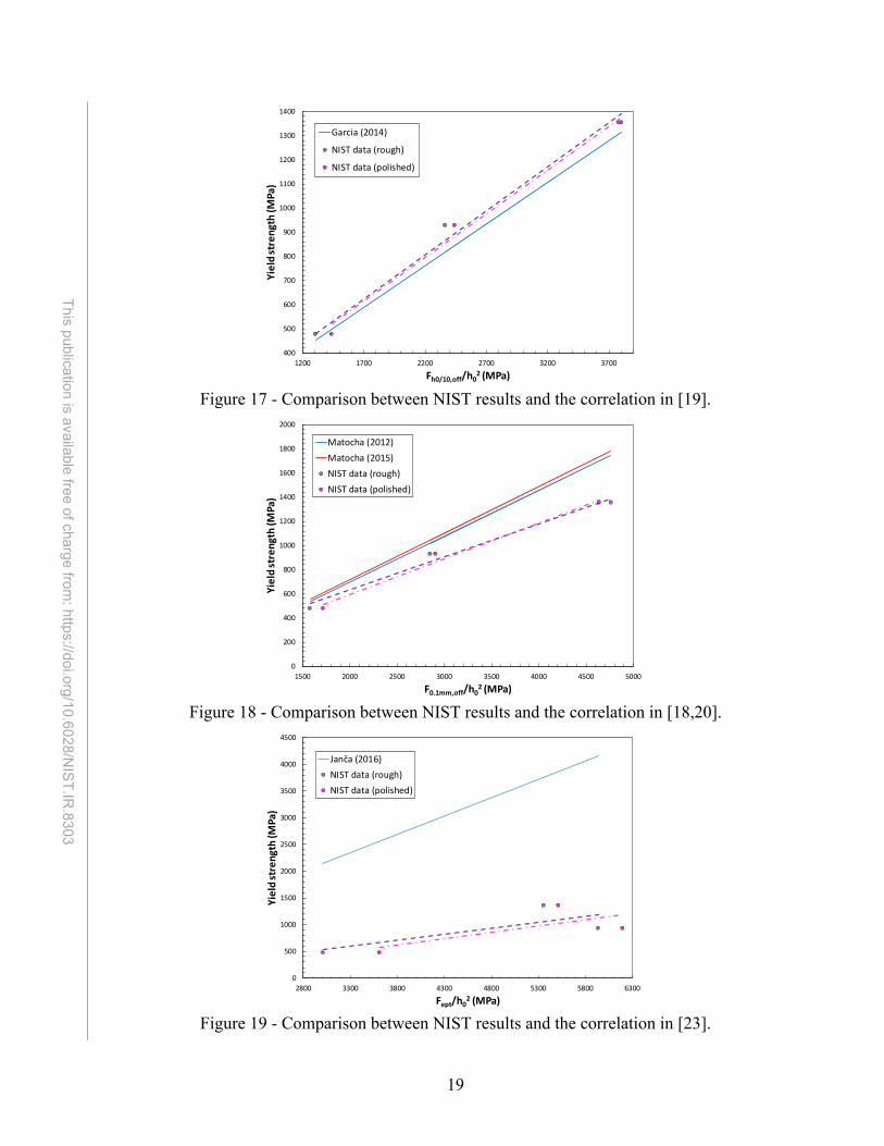
NIST correlations (for both rough and polished specimens) and literature correlations are compared in: • Fig. 15 (Eq. 17), • Fig. 16 (Eq. 18), • Fig. 17 (Eq. 19), • Fig. 18 (Eq. 20), • Fig. 19 (Eq. 21), • Fig. 20 (Eq. 22), and • Fig. 21 (Eq. 23).

18


IST.IR.8303

Figure 15 - Comparison between NIST results and the correlation in [24].


y = 1.764E+02e2.123E-04x

R² = 9.932E-01

y = 0.0059x1.2913

R² = 1

0

200

400

600

800

1000

1200

1400

1600

4000 6000 8000 10000 12000 14000

Yiel

d st

reng

th (M

Pa)

Slopeini/h0 (MPa)

Chica (2018)NIST data (rough)NIST data (polished)

400

500

600

700

800

900

1000

1100

1200

1300

1400

900 1100 1300 1500 1700 1900 2100 2300 2500 2700 2900

Yiel

d st

reng

th (M

Pa)

Fe(int)/h02 (MPa)

Garcia (2014)NIST data (rough)NIST (polished)

19


IST.IR.8303


Figure 18 - Comparison between NIST results and the correlation in [18,20].


400

500

600

700

800

900

1000

1100

1200

1300

1400

1200 1700 2200 2700 3200 3700

Yiel

d st

reng

th (M

Pa)

Fh0/10,off/h02 (MPa)

Garcia (2014)

NIST data (rough)

NIST data (polished)

0

200

400

600

800

1000

1200

1400

1600

1800

2000

1500 2000 2500 3000 3500 4000 4500 5000

Yiel

d st

reng

th (M

Pa)

F0.1mm,off/h02 (MPa)

Matocha (2012)Matocha (2015)NIST data (rough)NIST data (polished)

0

500

1000

1500

2000

2500

3000

3500

4000

4500

2800 3300 3800 4300 4800 5300 5800 6300

Yiel

d st

reng

th (M

Pa)

Fept/h02 (MPa)

Janča (2016)NIST data (rough)NIST data (polished)

20


IST.IR.8303



Our SP test results are in satisfactory agreement with the published models shown in Figs. 16, 17, and 18. Conversely, differences are significant with respect to the approaches illustrated in Figs. 15, 19, 20, and 21. As far as the correlations with Fept (Fig. 19) and Fe1.5 (Fig. 20) are concerned, the force values calculated from our tests showed significant scatter due to experimental noise, and are therefore associated to high uncertainties. The use of Eq. 22 and Eq. 23 is therefore not recommended. 7.2. Tensile strength correlations

Published correlations are split between authors who normalized Fm by the square of the initial thickness, ℎ02 [19,21,23], and those (the majority) who used the product between thickness and displacement at maximum force instead, h0∙um [17-23,25]. This latter approach appears justified by the observation that a significant specimen thinning has occurred at maximum force.

400

500

600

700

800

900

1000

1100

1200

1300

1400

900 1400 1900 2400 2900 3400 3900

Yiel

d st

reng

th (M

Pa)

Fe1.5/h02 (MPa)


400

600

800

1000

1200

1400

1600

1800

2000

2200

2200 2700 3200 3700 4200 4700 5200 5700 6200 6700 7200

Yiel

d st

reng

th (M

Pa)

F0.5mm/h02 (MPa)

Hähner (2019)NIST data (rough)NIST data (polished)

21


IST.IR.8303

Our results, shown in Fig. 22 and Fig. 24, fully confirm the higher reliability of the normalization by h0∙um. For normalization by ℎ02, the two empirical correlations we obtained:

𝑅𝑅𝑚𝑚 = 0.266 ∙ 𝐹𝐹𝑚𝑚ℎ02− 855.61 for rough specimens, and (24)

𝑅𝑅𝑚𝑚 = 0.152 ∙ 𝐹𝐹𝑚𝑚ℎ02− 228.73 for polished specimens (25)

have mediocre correlation coefficients (0.644 and 0.530, respectively), and are in poor agreement with similar models [19,21,23].

Figure 22 - Correlations between tensile strength and SP maximum force, normalized by ℎ02. The purple dashed line is the linear fit to the rough specimen data, while the pink dash-dotted

line is the linear fit to the polished specimen data.

On the other hand, our correlations between tensile strength and 𝐹𝐹𝑚𝑚ℎ0𝑢𝑢𝑚𝑚

:

𝑅𝑅𝑚𝑚 = 0.345 ∙ 𝐹𝐹𝑚𝑚ℎ0𝑢𝑢𝑚𝑚

− 42.84 for rough specimens, and (26)

𝑅𝑅𝑚𝑚 = 0.302 ∙ 𝐹𝐹𝑚𝑚ℎ0𝑢𝑢𝑚𝑚

+ 4.403 for polished specimens (27)

show a very strong degree of correlation (r = 0.944 and r = 1.000) and agree well with most of the published relationships [17-23,25] (Fig. 23). Published values of the coefficients of the linear regression (slope β1 and intercept β2) for steels were found to fall within the following intervals:

• Slope: β1 = 0.077 to 0.451. • Intercept11: β2 = -195.78 to 218.

11 Several authors forced the linear correlation through the origin, i.e., set β2 = 0.

500

700

900

1100

1300

1500

6000 6500 7000 7500 8000 8500 9000 9500 10000 10500

Tens

ile st

reng

th (M

Pa)

Fm/h02 (MPa)

Garcia (2014)Bruchhausen (2016)Janča (2016)NIST data (rough)NIST data (polished)

22


IST.IR.8303

Figure 23 - Correlations between tensile strength and SP maximum force, normalized by ℎ0𝑢𝑢𝑚𝑚.

Based on our literature search, the following additional SP forces were correlated with tensile strength in published papers: • Finfl (inflection point of the test record, where 𝑑𝑑

2𝐹𝐹𝑑𝑑𝑢𝑢2

= 0), normalized by ℎ0𝑢𝑢𝑚𝑚 [23], • F0.48mm (force corresponding to a punch displacement value of 0.48 mm), normalized by

ℎ02 [25], and • F0.65mm (force corresponding to a punch displacement value of 0.65 mm), normalized by

ℎ02 [23,26].

The following correlations were obtained by fitting our results on polished specimens (the results for rough specimens are reported in Annex 3) in accordance with the three approaches listed above.

𝑅𝑅𝑚𝑚 = 0.541 ∙ 𝐹𝐹𝑖𝑖𝑖𝑖𝑓𝑓𝑆𝑆ℎ0𝑢𝑢𝑚𝑚

+ 142.58 (r = 1.000) (28)

𝑅𝑅𝑚𝑚 = 0.246 ∙ 𝐹𝐹0.48𝑚𝑚𝑚𝑚ℎ02

+ 84.83 (r = 0.998) (29)

𝑅𝑅𝑚𝑚 = 0.230 ∙ 𝐹𝐹0.65𝑚𝑚𝑚𝑚ℎ02

− 59.9 (r = 0.998) . (30)

NIST correlations (for both rough and polished specimens) are compared to literature correlations in: • Fig. 24 (Eq. 28), • Fig. 25 (Eq. 29), and • Fig. 26 (Eq. 30).

200

400

600

800

1000

1200

1400

1600

1800

2000

1800 2300 2800 3300 3800 4300 4800

Tens

ile st

reng

th (M

Pa)

Fm/(h0um) (MPa)

Ruan (2002) Matocha (2012)Garcia (2014) Kumar (2015)Matocha (2015) Bruchhausen (2016)Altstadt (2016) Janča (2016)NIST data (rough) NIST data (polished)

23


IST.IR.8303



Figure 26 - Comparison between NIST results and the correlations in [23,26].

200

400

600

800

1000

1200

1400

1600

800 1300 1800 2300 2800

Tens

ile st

reng

th (M

Pa)

Finfl/(h0um) (MPa)


200

400

600

800

1000

1200

1400

1600

1800 2800 3800 4800 5800 6800

Tens

ile st

reng

th (M

Pa)

F0.48mm/h02 (MPa)

Kumar (2015)

NIST data (rough)


0

500

1000

1500

2000

2500

3000

3500

4000

2800 3300 3800 4300 4800 5300 5800 6300 6800 7300 7800

Tens

ile st

reng

th (M

Pa)

F0.65mm/h02 (MPa)

Janča (2016)Altstadt (2018)NIST data (rough)NIST data (polished)

24


IST.IR.8303

Another correlative approach [33] was proposed, based on normalizing Fm by (A + B∙um), where A and B are least-squares regression coefficients. We obtained (Fig. 27):

𝑅𝑅𝑚𝑚 = 𝐹𝐹𝑚𝑚0.885−815.35∙𝑢𝑢𝑚𝑚

for polished specimens (r = 0.589). (31)


For all these alternative approaches, the agreement between our analyses and the literature is not satisfactory, with the exception of Altstadt’s model [26] in Fig. 26. 7.3. Total elongation correlations

Our literature search identified three distinct empirical correlations for total elongation: the first [19,27] simply converted displacement at maximum force, um, into εt, the second [19,28] used um normalized by the initial thickness h0, and the third [29] established a linear regression of the form 𝜀𝜀𝑑𝑑 = 𝜔𝜔1

𝑢𝑢𝑓𝑓−ℎ0ℎ0

+ 𝜔𝜔2, using punch displacement at test end, uf. Our test results yielded the following correlations for polished specimens:

𝜀𝜀𝑑𝑑 = 16.045 ∙ 𝑢𝑢𝑚𝑚 (r = 0.839) (32)

𝜀𝜀𝑑𝑑 = 7.22 ∙ 𝑢𝑢𝑚𝑚ℎ0

(r = 0.836) (33)

𝜀𝜀𝑑𝑑 = 8.334 ∙ 𝑢𝑢𝑓𝑓−ℎ0ℎ0

+ 2.05 (r = 0.959) . (34)

These correlations are compared to published relationships [19, 27-29] in Figs. 28-30. Note that most of the published correlations were established with measurements of specimen deflection, and therefore the comparisons shown in Figs. 28-30 are only qualitative.

500

700

900

1100

1300

1500

1500 1700 1900 2100 2300 2500

Tens

ile st

reng

th (M

Pa)

Fm (N)

Holmström (2019)NIST data (rough)NIST data (polished)

25


IST.IR.8303

Figure 28 - Comparison between NIST results and the correlations in [19,27] for εt.

Figure 29 - Comparison between NIST results and the correlations in [19,28] for εt.

Figure 30 - Comparison between NIST results and the correlation in [29] for εt.

10

12

14

16

18

20

22

24

26

28

0.8 0.9 1 1.1 1.2 1.3 1.4 1.5 1.6 1.7

Tota

l elo

ngat

ion

(%)

um (mm)

Fleury-Ha (1998)Garcia (2014)NIST data (rough)NIST data (polished)

10

12

14

16

18

20

22

24

26

1.6 1.8 2 2.2 2.4 2.6 2.8 3 3.2 3.4

Tota

l elo

ngat

ion

(%)

um/h0

Rodriguez (2009)Garcia (2014)NIST data (rough)NIST data (polished)

-100

-80

-60

-40

-20

0

20

40

1 1.2 1.4 1.6 1.8 2 2.2 2.4 2.6 2.8 3

Tota

l elo

ngat

ion

(%)

(uf-h0)/h0

Yang (2018)

NIST data (rough)


26


IST.IR.8303

Additional correlations (not previously published)

In this study, we also attempted to establish correlations between our SP test results and two other mechanical parameters, for which no relationships exist based on our bibliographic search: uniform elongation, εu, and Charpy absorbed energy, KV.

8.1. Uniform elongation In the case of uniform elongation (which is calculated at maximum force), our

correlations were established with um normalized by h0 (Fig. 31):

𝜀𝜀𝑢𝑢 = 6.276 ∙ 𝑢𝑢𝑚𝑚ℎ0− 7.55 for rough specimens, and (35)

𝜀𝜀𝑢𝑢 = 5.380 ∙ 𝑢𝑢𝑚𝑚ℎ0− 6.43 for polished specimens. (36)

The correlation coefficients are 0.976 for Eq. 35 and 0.968 for Eq. 36, showing in both cases a strong degree of linear correlation.

Figure 31 - Correlations between uniform elongation and 𝑢𝑢𝑚𝑚

ℎ0 obtained at NIST.

8.2. Charpy absorbed energy For rough specimens, the strongest correlation with KV was obtained with EPL (r =

0.924): 𝐾𝐾𝐾𝐾 = 522.90 ∙ 𝐸𝐸𝑆𝑆𝑃𝑃 − 354.1 , (37)

but the correlations with ESP and Em are also fairly strong (r = 0.785 and r = 0.834, respectively). More details can be found in Annex 3. In the case of polished specimens, the strongest linear relationship was found between KV and ESP (r = 0.956):

𝐾𝐾𝐾𝐾 = 289.21 ∙ 𝐸𝐸𝑆𝑆𝑃𝑃 − 438.8 , (38) while the remaining two are poor (r = 0.484 for KV vs. Em and r = 0.436 for KV vs. EPL). The two correlations (Eqs. 37 and 38) are illustrated in Fig. 32.

2.5

4.5

6.5

8.5

10.5

12.5

1.6 1.8 2 2.2 2.4 2.6 2.8 3 3.2 3.4

Uni

form

elo

ngat

ion

(%)

um/h0

NIST (rough)NIST (polished)

27


IST.IR.8303

Figure 32 - Correlations between Charpy absorbed energy and SP energies for rough and

polished specimens.

Discussion: effect of specimen surface finish In order to assess the influence of surface finish on the results of SP tests, we ran two-

sample t-tests [34] on the mean values of selected SP characteristic values (Fe, Fm, ue, um, uf, and ESP) obtained from rough (Ra = 3 µm to 4 µm) and polished (Ra = 0.05 µm to 0.25 µm) specimens. Specifically, we statistically tested the null hypothesis that the means for rough and polished specimens are equal (tcalc < tcritical).

The results of the t-tests for the three steels are summarized in Table 11.

Table 11 - Influence of specimen surface finish on SP test results: results of two-sample t-tests on means12 of characteristic parameters.

Steel Surface finish

Fe,mean (N)

Fm,mean (N)

ue,mean (mm)

um,mean (mm)

uf,mean (mm)

ESP,mean (J)

JRQ

Rough 247.0 1563.3 0.113 1.637 1.870 1.87 Polished 257.7 1742.1 0.086 1.657 1.971 2.27

tcalc 1.21 18.17 2.94 1.04 3.63 11.13 tcritical 2.06 2.06 2.06 2.06 2.06 2.06

Different? NO YES YES NO YES YES

4340LL

Rough 651.3 1896.1 0.141 0.854 1.059 1.41 Polished 652.7 2121.2 0.100 0.857 1.098 1.66

tcalc 0.05 9.19 4.71 0.14 1.48 4.67 tcritical 2.11 2.11 2.11 2.11 2.11 2.11

Different? NO YES YES NO NO YES

4340HH

Rough 448.6 2113.2 0.124 1.239 1.331 1.63 Polished 434.9 2491.2 0.090 1.442 1.583 2.42

tcalc 1.08 10.32 7.16 7.44 7.94 14.00 tcritical 2.10 2.10 2.10 2.10 2.11 2.10

Different? NO YES YES YES YES YES

12 If tcalc > tcritical, the means of the two populations are statistically different (at a significance level α = 0.05).

0

50

100

150

200

0.5 0.7 0.9 1.1 1.3 1.5 1.7 1.9 2.1 2.3 2.5

Char

py a

bsor

bed

ener

gy (J

)

SP energies (J)

NIST (rough) - E_PLNIST (polished) - E_SP

28


IST.IR.8303

Based on the results of the t-tests, specimen surface finish does not have a significant influence on elastic-plastic transition forces, but does affect significantly maximum forces, displacements at elastic-plastic transition, and fracture energies for all the steels considered. The effect is particularly strong on Fm and ESP (tcalc >> tcritical), with lower surface roughness leading to significantly higher values of force and energy. The results are less clear-cut for the remaining parameters (ue and uf), where the influence of surface finish seems to depend on the material.

Conclusions

The Small Punch test technique was developed at NIST to investigate the mechanical properties of metallic materials through the use of a minimal amount of material. This technique was successfully qualified by running tests on three steels (A533B and 4340 with two distinct heat treatments) spanning a large range of tensile and fracture properties (Table 2).

NIST SP test results on the JRQ (A533B) steel were successfully compared to data collected in an international round-robin that was conducted in 2017 in support of the development of an ASTM Test Method.

Empirical correlations were established between SP characteristic parameters (forces and punch displacements) and tensile properties (yield and ultimate tensile strengths, uniform and total elongations) for the three steels investigated. Most of the relationships obtained showed a strong degree of linear correlation and were found to be in satisfactory agreement with published empirical correlations.

Finally, we studied the effect of specimen surface finish on SP results, by testing “rough” (Ra = 3 µm to 4 µm) and “polished” (Ra = 0.05 µm to 0.25 µm) samples. A lower surface roughness yielded statistically higher values of most SP characteristic parameters, particularly at maximum force and in terms of energy. Conversely, elastic-plastic transition forces were substantially independent of surface finish for the materials and conditions investigated. Moreover, relationships from polished specimens exhibited generally higher degrees of correlation than those from rough specimens, therefore supporting the requirement Ra < 0.25 µm in [10,11].

References

[1] Lucon, E., 2014, “Testing of Small-Sized Specimens,” Comprehensive Materials Processing. C. J. Van Tyne, ed., Elsevier Ltd., Vol. 1, pp. 135-163.

[2] Harling, O. K., Lee, M., Sohn, D.-S., Kohse, G., and Lau, C. W., 1986, “The MIT Miniaturised Disc Bend Test,” The Use of Small-Scale Specimens for Testing Irradiated Material, ASTM STP 888. W. R. Corwin, and G. E. Lucas, eds., ASTM, Philadelphia, PA, pp. 50–65.

[3] Manahan, M. P., Browning, A. E., Argon, A. S., and Harling, O. K., 1986, “Miniaturised Disc Bend Test Technique Development and Application,” The Use of Small-Scale Specimens for Testing Irradiated Material, ASTM STP 888. W. R. Corwin, and G. E. Lucas, eds., ASTM, Philadelphia, PA, pp. 17–49.

[4] Hankin, G. L., Toloczko, M. B., Hamilton, M. L., Garner, F. A., and Faulkner, R. G., 1998, “Validation of the Shear Punch – Tensile Correlation Technique Using Irradiated Materials,” Journal of Nuclear Materials, 258–263, pp. 1651–1656.

29


IST.IR.8303

[5] Bicego, V., Lucon, E., and Sampietri, C., 1998, “The ‘Small Punch’ Technique for Evaluating Quasi Non-Destructively the Mechanical Properties of Steels.” In Fracture from Defects, ECF 12: Proceedings of the Twelfth European Conference on Fracture. M. W. Brown, E. R. de los Rios, K. J. Miller, eds., EMAS Publishing, London, Vol. 1, pp 1273–1278.

[6] Sainte-Catherine, C., Messier. J., Poussard, C., Rosinski, S., and Foulds, J., 2002, “Small Punch Test: EPRI-CEA Finite Element Simulation Benchmark and Inverse Method for the Estimation of Elastic Plastic Behavior,” in Small Specimen Test Techniques: Fourth Volume, ASTM STP 1418, M. A. Sokolov, J. D. Landes, and G. E. Lucas, Eds., ASTM International, West Conshohocken, PA, pp. 350-370.

[7] Abendroth, M. and Kuna, M., “Determination of Deformation and Failure Properties of Ductile Materials by Means of the Small Punch Test and Neural Networks,” Computational Materials Science, Vol 28, 2003, pp. 633-644.

[8] Abendroth, M. and Kuna, M., 2004, “Determination of Ductile Material Properties by Means of the Small Punch Test and Neural Networks,” Advanced Engineering Materials, Vol 6, No. 7, 2004, pp. 536-540.

[9] Kuna, M. and Abendroth, M., 2012, “Identification and Validation of Ductile Damage Parameters by the Small Punch Test,” in Proceedings of the 2nd International Conference SSTT, Determination of Mechanical Properties of Materials by Small Punch and Other Miniature Testing Techniques, Oct 2-4. 2012, Ostrava, Czech Republic, Ocelot Publ., ISBN 978-80-260-0079-2, pp. 4-18.

[10] CEN Workshop Agreement, CWA 15627:2007, “Small Punch Test Method for Metallic Materials,” European Committee for Standardization, Brussels, Belgium.

[11] ASTM Subcommittee E10.02, 2019, “Standard Test Method for Small Punch Testing of Metallic Materials,” Work Item WK61832, Version 01/29/19.

[12] International Atomic Energy Agency, 2001, “Reference manual on the IAEA JRQ correlation monitor steel for irradiation damage studies,” IAEA, Vienna, Austria.

[13] Brumovski, M. and Kopriva, R., 2018, “Interlaboratory Study for Small Punch Testing Preliminary Results,” Proceedings of the ASME 2018 Pressure Vessels and Piping Conference, PVP2018, July 15-20, 2018, Prague, Czech Republic.

[14] McCowan, C.N., Siewert, T.A., and Vigliotti, D.P., 2003, “Charpy verification program: reports covering 1989-2002,” NIST Technical Note 1500-9, Materials Reliability Series.

[15] Lucon, E., 2016, "Estimating dynamic ultimate tensile strength from instrumented Charpy data," Materials & Design, Volume 97, pp. 437-443.

[16] Lucon, E., 2019, “Use and Validation of the Slope Determination by the Analysis of Residuals (SDAR) Algorithm,” NIST Technical Note 2050.

[17] Ruan, Y., Spätig, P., and Victoria, M., 2002, “Assessment of mechanical properties of the martensitic steel EUROFER97 by means of punch tests,” Journal of Nuclear Materials, 307-311, pp. 236–239.

[18] Matocha, K., 2012, “Determination of actual tensile and fracture characteristics of critical components of industrial plants under long term operation by SPT,” Proceedings of the ASME 2012 Pressure Vessels & Piping Conference, PVP2012, Toronto, Canada, July 15-19, ASME Paper No. PVP2012-78553.

[19] García, T.E., Rodríguez, C., Belzunce, F.J., and Suárez, C., 2014, “Estimation of the mechanical properties of metallic materials by means of the small punch test,”

30


IST.IR.8303

Journal of Alloys and Compounds, 582, pp. 708-717. [20] Matocha, K., 2015, “Small-Punch Testing for Tensile and Fracture Behavior:

Experiences and Way Forward,” Small Specimen Test Techniques: 6th Volume, ASTM STP 1576. M. A. Sokolov and E. Lucon, eds., West Conshohocken, PA, pp. 145–159.

[21] Bruchhausen, M., Holmström, S., Simonovski, I., Austin, T., Lapetite, J.-M., Ripplinger, J.-M., and de Haan, F., 2016, “Recent developments in small punch testing: Tensile properties and DBTT,” Theoretical and Applied Fracture Mechanics, 86, pp. 2–10.

[22] Altstadt, E., Ge, H.E., Kuksenko, V., Serrano, M., Houska, M., Lasan, M., Bruchhausen, M., Lapetite, and Dai, Y., 2016, “Critical evaluation of the small punch test as a screening procedure for mechanical properties,” Journal of Nuclear Materials, 472, pp. 186–195.

[23] Janča, A., Siegl, J., and Haušild, P., 2016, “Small punch test evaluation methods for material characterization,” Journal of Nuclear Materials, 481, pp. 201–213.

[24] Chica, J.C., Díez, P.M.B., and Calzada, M.P., 2018, “Development of an improved correlation method for the yield strength of steel alloys in the small punch test.” Proceedings of 5th International Small Sample Test Techniques, SSTT2018, Swansea University, UK, July 10-12, 2018, Ubiquity Proceedings.

[25] Kumar, K., Pooleery, A., Madhusoodanan, K., Singh, R.N., Chakravartty, J.K., Shriwastaw, R.S., Dutta, B.K., and Sinha, R.K., 2015, “Evaluation of ultimate tensile strength using Miniature Disk Bend Test,” Journal of Nuclear Materials, 461, pp. 100–111.

[26] Altstadt, E., Houska, M., Simonovski, I., Bruchhausen, M., Holmström, S., and Lacalle, R., 2018, “On the estimation of ultimate tensile stress from small punch testing,” International Journal of Mechanical Sciences, 136, pp. 85–93.

[27] Fleury, E. and Ha, J.S., 1998, “On the estimation of ultimate tensile stress from small punch testing,” International Journal of Pressure Vessels and Piping, 75, pp. 699–706.

[28] Rodriguez, C., Garcia Cabezas, J., Cardenas, E., Belzunce, F. J., and Betegon, C., 2009, “Mechanical Properties Characterization of Heat-Affected Zone Using the Small Punch Test,” Welding Research, Vol. 88, pp. 188-s–192-s.

[29] Yang, S., Ling, X., and Peng, D., 2018, “Elastic and plastic deformation behavior analysis in small punch test for mechanical properties evaluation,” Journal of Central South University, 25(4), pp. 747–753.

[30] Hähner, P., Soyarslan, C., Gülçimen Çakan, B., and Bargmann, S., 2019, “Determining tensile yield stresses from Small Punch tests: A numerical-based scheme,” Material and Design, 182, 107974.

[31] Contreras, M.A., Rodríguez, C., Belzunce, F. J., and Betegón, C., 2008, “Use of the small punch test to determine the ductile‐to‐brittle transition temperature of structural steels,” Fatigue & Fracture of Engineering Materials & Structures.

[32] Matocha, K. 2015, “Small Punch Testing for Tensile and Fracture Behavior: Experiences and Way Forward,” Small Specimen Test Techniques: 6th Volume. STP 1576, Mikhail Sokolov and Enrico Lucon, Eds. ASTM International, West Conshohocken, PA, pp. 145-159.

31


IST.IR.8303

[33] Holmström, S., Simonovski, I., Baraldi, D., Bruchhausen, M., Altstadt, E., Delville, R., 2019, “Developments in the estimation of tensile strength by small punch testing,” Theoretical and Applied Fracture Mechanics, Volume 101, pp. 25-34.

[34] NIST/SEMATECH e-Handbook of Statistical Methods, http://www.itl.nist.gov/div898/handbook/, update April 2012.

http://www.itl.nist.gov/div898/handbook/


IST.IR.8303

Annex 1

Operational Procedure for Performing Small Punch Tests at NIST in Boulder, Colorado


IST.IR.8303

This Operational Procedure implies the use of the MTS servo-hydraulic 858 Mini Bionix II machine13, equipped with a 5 kN calibrated load cell, for Small Punch testing, along with an Epsilon extensometer for measuring punch displacement. Additionally, the MTS TestStar IIs Station Manager, Version 4.0, should be used to operate the machine.

In “Station Manager”:

• Select Project: Project 1 • Open Station: Basic (5 kN Load Cell) • Open Procedure: smallpunch.000.

Pre-Test Operations

1. Turn on high pressure for the pumps (HPS1, HSM1).

2. In the “Manual Command” window, check that manual command is enabled, then select (actuator) displacement control.

3. Enter 25 mm as the value of displacement, thus making the actuator rise.

4. Insert snugly the SP specimen into the lower die. If burrs are present that prevent complete introduction of the specimen, remove them by the use of sand paper.

5. Place the upper die onto the lower die, and hand-tighten the four screws.

6. Drop the steel ball into the hole on the top of the upper die.

7. Place the steel rod into the hole, on top of the steel ball.

8. Place the whole fixture in the machine, by inserting the rod into the hole of the upper machine thread, and holding it manually in place.

9. In the “Manual Command” window, enter 5 mm as displacement, then slowly approach the SP fixture to the lower machine plate by clicking on the left slider bar until the top of the rod is very close to the bottom of the hole in the upper machine thread. At the very end of the process, click on the left arrow to achieve smaller displacements and avoid accidentally overloading the specimen.

10. Tighten the whole setup by turning clockwise the upper machine thread until a force in the range -15 kN to -30 kN is attained (check the force in the window “Meters”).

11. In the window “Signal Auto Offset”, zero Axial Displacement.

12. Approach the extensometer to its working position, and take the safety pin out. Verify that in the window “Meters 1”, the last two digits of the extensometer signal keep changing. NOTE: if the digits do not change, the extensometer may be out of range and no signal will be recorded. If that is the case. adjust the extensometer until you see variation in the last two digits of the signal.

13 Certain commercial equipment, instruments, or materials are identified in this document in order to specify the experimental procedure adequately. Such identification is not intended to imply recommendation or endorsement by the National Institute of Standards and Technology, nor is it intended to imply that the materials or equipment identified are necessarily the best available for the purpose.


IST.IR.8303

13. In the window “Signal Auto Offset”, zero Extensometer.

14. Input the specimen name/id in Station Manager.

15. Uncheck manual command in the window “Manual Command”.

Test Operations 1. Click the big white arrow in Station Manager.

2. Input all the test information in the “Procedure / User Input” window.

3. After clicking OK, the test starts and the Force-Displacement and Force-Extensometer plots are visualized. NOTE: force, displacement, and extensometer values will be plotted with their actual sign (negative for compression tests).

Post-Test Operations

1. Once the test is finished (the red square in Station Manager is highlighted), click “New Specimen”. The two plots close.

2. In the “Manual Command” window, select manual command and (actuator) displacement control.

3. Move the extensometer away from the actuator and put the safety pin back in place.

4. In the “Manual Command” window, enter 25 mm as the value of displacement, making the actuator rise.

5. Remove the assembly/fixture from the machine.

6. Extract the rod from the fixture.

7. Disassemble upper and lower die by unscrewing and removing the 4 screws.

8. Take the ball out and store it.

9. Remove the specimen.

End of Testing Operations

Turn the pumps off (HPS1, HSM1).


IST.IR.8303

Annex 2

Spreadsheet-Based Software for the Analysis of a Small Punch Test


IST.IR.8303

The analyses of Small Punch tests in this study were performed by means of a Microsoft Excel14 macro-enabled spreadsheet, which can be distributed free of charge to anyone interested by requesting a copy from [email protected].

Preliminary Operations

The first worksheet (“Data”, Fig. A2-1) contains the raw data of the test (time, actuator displacement, extensometer displacement, force). Before pasting data from a new test, columns A-D can be cleared by clicking the button CLEAR DATA at the top (circled in red in Fig. A2-1). The raw data for the new test should be pasted as values in columns A-D, starting in row 15 (highlighted in yellow). After pasting the data, the user should make sure that the length of columns E-K is the same as columns A-D, by either removing empty rows or copying the information through the last data row.

Figure A2-1 – Worksheet “Data”.

NOTE: actuator displacement, extensometer displacement, and force data acquired during a SP test at NIST are negative, as the tests are in compression. Columns E-G simply reverse the sign of the values. Should raw data have a positive sign, the formulas in columns E-G ought to be correspondingly modified.

General information for the test (operator, project, specimen id, material information, initial specimen thickness h0, optional notes) can be entered in cells B4-B9 (highlighted in yellow and outlined in green in Fig. A2-1). Some of this information is automatically transferred into cells O8-O11, to be printed along with the test results.

Make sure that the system compliance values for the actuator and extensometer signals, in mm/N, are entered correctly in cells J2-J3 (circled in blue in Fig A2-1).

14 Certain commercial software, equipment, instruments or materials are identified in this report to adequately specify the experimental procedure. Such identification is not intended to imply recommendation or endorsement by the National Institute of Standards and Technology, nor is it intended to imply that the equipment or materials identified are necessarily the best available for the purpose.

mailto:[email protected]


IST.IR.8303

Next, define the lower and upper limit of the initial linear portion of the test record, in N, by looking at the curves in the worksheet “Test Record”, and input them in cells T3-T4 (highlighted in yellow and circled in purple in Fig. A2-1). The corresponding calculated offset values for the force-displacement and force-actuator curves are displayed in cells O3-O4.

Determination of the Elastic-Plastic Transition Force, Fe

Select the worksheet “ASTM analyses (Fe)” (Fig. A2-2). Columns A and B contain raw displacement and force data up to u = 0.5 mm, automatically copied from the “Data” worksheet.

In cell J2 (highlighted in yellow and circled in red in Fig. A2-2), enter “0.25”. In cells M2-M3 (highlighted in yellow and circled in green in Fig. A2-2), enter the approximate force values corresponding to u = 0.25 mm and u = 0.5 mm, respectively. To estimate these forces, look at the diagram in the worksheet “Fe determination (ASTM)”.

Enter in cell U2, in N, (highlighted in yellow and circled in blue in Fig. A2-2) the lower force limit, below which data should not be included in the linear fit of the initial portion of the test record. This avoids including any initial non-linearities in the first linear regression.

Click the button PERFORM CALCULATIONS. The bilinear model of the ASTM Draft Test Method [11] is applied by minimizing the error in cell M8 (highlighted in pink) by the use of the SOLVER tool of Microsoft Excel.

The calculations in this worksheet yield the values of [ue,Fe], [u0.1mm,off,F0.1mm,off], and [uh0/10,off,Fh0/10,off] in column P.

Figure A2-2 – Worksheet “ASTM analyses (Fe)”.

Check the plot in the worksheet “Fe determination (ASTM)” (Fig A2-3) and, if necessary, adjust the axis scales and/or the position of the text labels.


IST.IR.8303

Figure A2-3 – Worksheet “Test record”.

Final Operations and Test Results Printing

Select the worksheet “Test record” and, if necessary, adjust the axis scales and/or the position of the text labels. The data points visualized on this plot are Fe, Fm, and Ff (in reference to the blue punch displacement curve, Fig. A2-4).

Figure A2-4 – Worksheet “Test record”.

To print out the complete test results on the default system printer, click PRINT RESULTS in the “Data” worksheet (outlined in orange in Fig. A2-1).

0

100

200

300

400

500

600

700

0 0.05 0.1 0.15 0.2 0.25 0.3 0.35 0.4 0.45 0.5

Forc

e (N

)

Displacement (mm)

uA = uE

fA

Fe

0

200

400

600

800

1000

1200

1400

1600

1800

2000

0 0.5 1 1.5 2 2.5

Forc

e (N

)

Displacement (mm)



um

Fm

Fe

Ff

uf


IST.IR.8303

Three pages are printed: a summary of the numerical results (test info, forces, displacements, and energies, see Fig. A2-5), the test record (Fig. A2-4), and the graphical results for the determination of Fe (worksheet “Fe determination (ASTM)”, Fig. A2-3).

Figure A2-5 – Test results printout.


IST.IR.8303

Annex 3

Summary of Correlations between SP Parameters and Tensile Properties

(from the Literature, 1998-2019, and Obtained at NIST)


IST.IR.8303

Small Punch-Tensile Property Correlations

Yield Strength correlations

Characteristic SP force: Fe,proj (two tangents, projection – CWA 15267 & ASTM Draft) 𝑅𝑅𝑝𝑝02 = 𝛼𝛼1𝐹𝐹𝑒𝑒,𝑆𝑆𝑝𝑝𝑆𝑆𝑝𝑝

ℎ02+ 𝛼𝛼2

𝛼𝛼1 𝛼𝛼2 Reference Notes

0.413 149 [17] EUROFER97

0.5892 -77.136 [18] 14MoV6-3 steel

0.476 0 [19]

0.4334 -67.041 [20]

0.382 28.8 [21]

0.884 0 [22] T91 steel

0.575 -34 [23]

0.5460 0.5282

-35.7 0 NIST [rough]

A533B (JRQ) & 4340 steels 0.5379

0.5125 -52.2

0 NIST [polished]

Characteristic SP force: Fe,int (two tangents, intersection) 𝑅𝑅𝑝𝑝02 = 𝛼𝛼1𝐹𝐹𝑒𝑒,𝑖𝑖𝑖𝑖𝑖𝑖ℎ02

+ 𝛼𝛼2


0.442 0 [19]

0.503 0.474

0 0

NIST [rough] NIST [polished]

A533B (JRQ) & 4340 steels

Characteristic SP force: Fh0/10,off (offset, punch displacement t/10 ≈ 0.05 mm) 𝑅𝑅𝑝𝑝02 = 𝛼𝛼1𝐹𝐹ℎ0/10,𝑆𝑆𝑓𝑓𝑓𝑓

ℎ02+ 𝛼𝛼2


0.346 0 [19]

0.366 0.362

0 0




IST.IR.8303

Characteristic SP force: F0.1mm,off (offset, punch displacement = 0.1 mm) 𝑅𝑅𝑝𝑝02 = 𝛼𝛼1𝐹𝐹0.1𝑚𝑚𝑚𝑚,𝑆𝑆𝑓𝑓𝑓𝑓

ℎ02+ 𝛼𝛼2


0.3797 -64.18 [18] 14MoV6-3 steel

0.385 -55.61 [20]

0.2713 0.2962

88.49 5.35



Characteristic SP force: Fept (max curvature in force/displacement curve) 𝑅𝑅𝑝𝑝02 = 𝛼𝛼1𝐹𝐹𝑒𝑒𝑆𝑆𝑖𝑖ℎ02

+ 𝛼𝛼2


0.69 56 [23]

0.2171 0.2358

-114.96 -284.78



Characteristic SP force: Fe1.5 (Area under curve/Area above curve = 1.5) 𝑅𝑅𝑝𝑝02 = 𝛼𝛼1𝐹𝐹𝑒𝑒1.5

ℎ02+ 𝛼𝛼2


0.51 91 [23]

0.4275 0.3101

137.84 204.61



Characteristic SP forces: F0.1mm, F0.5mm, F0.9mm (punch displacements = 0.1 mm, 0.5 mm, 0.9 mm)

Equations Reference Notes

𝐾𝐾 =(𝐹𝐹0.5𝑚𝑚𝑚𝑚 − 𝐹𝐹0.1𝑚𝑚𝑚𝑚) − (𝐹𝐹0.9𝑚𝑚𝑚𝑚 − 𝐹𝐹0.5𝑚𝑚𝑚𝑚)

𝐹𝐹0.9𝑚𝑚𝑚𝑚 − 𝐹𝐹0.1𝑚𝑚𝑚𝑚

For K < 0.33: 𝑅𝑅𝑝𝑝02 = (1.28𝐾𝐾 − 0.062) 𝐹𝐹0.5𝑚𝑚𝑚𝑚ℎ02

For K ≥ 0.33: 𝑅𝑅𝑝𝑝02 = 0.36 𝐹𝐹0.5𝑚𝑚𝑚𝑚ℎ02

[30] K = curvature

𝑅𝑅𝑝𝑝02 = 0.2387𝐹𝐹0.5𝑚𝑚𝑚𝑚

ℎ02− 61.938

𝑅𝑅𝑝𝑝02 = 0.2055𝐹𝐹0.5𝑚𝑚𝑚𝑚

ℎ02− 60.920

NIST [rough]

NIST [polished]



IST.IR.8303

Characteristic SP values: Slopeini (slope initial region SP curve – Zone I) 𝑅𝑅𝑝𝑝02 = 𝛾𝛾1𝑒𝑒𝛾𝛾2∙

𝑆𝑆𝑆𝑆𝑆𝑆𝑆𝑆𝑒𝑒𝑖𝑖𝑖𝑖𝑖𝑖ℎ0

𝛾𝛾1 𝛾𝛾2 Reference Notes

47.41 1.736 ⋅ 10-4 [24]

176.42 0.0059

2.123 ∙ 10-4

1.2913 NIST [rough]

NIST [polished] A533B (JRQ) & 4340 steels


IST.IR.8303

Tensile Strength correlations

Characteristic SP force: Fm 𝑅𝑅𝑚𝑚 = 𝛽𝛽1𝐹𝐹𝑚𝑚ℎ02

+ 𝛽𝛽2

𝛽𝛽1 𝛽𝛽2 Reference Notes

0.065 268.81 [19]

0.093 -11.86 [21]

0.08 250 [23]

0.2662 0.1523

-855.61 -228.73



Characteristic SP force: Fm 𝑅𝑅𝑚𝑚 = 𝛽𝛽1𝐹𝐹𝑚𝑚

ℎ0𝑢𝑢𝑚𝑚+ 𝛽𝛽2


0.077 218 [17] EUROFER97

0.451 -93.46 [18] 14MoV6-3 steel

0.277 0 [19]

0.130 0 [25]

0.4335 -195.78 [20]

0.326 -27.04 [21]

0.279 0 [22]

0.201 108 [23]

0.3453 0.3024

-42.84 4.403



Characteristic SP force: Fm 𝑅𝑅𝑚𝑚 = 𝐹𝐹𝑚𝑚𝐴𝐴+𝐵𝐵𝑢𝑢𝑚𝑚

𝐴𝐴 𝐵𝐵 Reference Notes

0.6143 1.2954 [33] MCH model

0.9386 0.8845

-675.83 -815.35




IST.IR.8303

Characteristic SP force: Finfl (inflection point, 𝑑𝑑2𝐹𝐹

𝑑𝑑𝑢𝑢2 = 0) 𝑅𝑅𝑚𝑚 = 𝛽𝛽1

𝐹𝐹𝑖𝑖𝑖𝑖𝑓𝑓𝑆𝑆ℎ0𝑢𝑢𝑚𝑚

+ 𝛽𝛽2


0.207 48 [33]

0.5413 0.6122

142.58 -226.39



Characteristic SP force: F0.48mm (punch displacement = 0.48 mm) 𝑅𝑅𝑚𝑚 = 𝛽𝛽1𝐹𝐹0.48𝑚𝑚𝑚𝑚

ℎ02+ 𝛽𝛽2


0.13 6 [25]

0.2456 0.2098

84.829 92.13




ℎ02+ 𝛽𝛽2


0.51 91 [23]

0.2298 0.2115

-59.9 -113.94




ℎ02+ 𝛽𝛽2


0.179 0 [26] ALT model

0.2298 0.2115

-59.9 -113.94




IST.IR.8303

Total Elongation correlations

Characteristic SP parameter: um 𝐴𝐴 [%] = 𝜔𝜔1𝑢𝑢𝑚𝑚

𝜔𝜔1 Reference Notes

14 [27]

12.57 [19]

16.492 16.045



Characteristic SP parameter: um 𝐴𝐴 [%] = 𝜔𝜔1𝑢𝑢𝑚𝑚ℎ0

𝜔𝜔1 Reference Notes

7 [28]

6.07 [19]

7.81 7.22



Characteristic SP parameter: uf 𝐴𝐴 [%] = 𝜔𝜔1𝑢𝑢𝑓𝑓−ℎ0ℎ0

+ 𝜔𝜔2

𝜔𝜔1 𝜔𝜔2 Reference Notes

0.338 -88.08 [29] AISI 304

9.0413 8.3341

2.54 2.05



Uniform Elongation correlations

Characteristic SP parameter: um 𝜀𝜀𝑢𝑢 [%] = 𝜔𝜔1𝑢𝑢𝑚𝑚ℎ0

+ 𝜔𝜔2

𝜔𝜔1 𝜔𝜔2 Reference Notes

6.2756 5.3804

-7.5548 -6.4341



development and validation of small punch testing at nist

Documents