development and integration of a sun sensor for the pico-satellite...
TRANSCRIPT

Supervision: Dipl.-Ing. Claas Olthoff Lehrstuhl für Raumfahrttechnik / Institute of Astronautics Technische Universität München Stefan Mahnke Otto-von-Taube-Gymnasium Gauting
Lehrstuhl für Raumfahrttechnik Prof. Dr. rer. nat. Ulrich Walter
Seminararbeit
Development and Integration of a Sun Sensor for the Pico-Satellite MOVE
Author:
Dominik von Mengden

Development and Integration of a Sun Sensor for the Pico-Satellite MOVE Dominik von Mengden
Page II
Erklärung
Ich erkläre, dass ich alle Einrichtungen, Anlagen, Geräte und Programme, die mir im Rahmen meiner Semester- oder Diplomarbeit von der TU München bzw. vom Lehrstuhl für Raumfahrttechnik zur Verfügung gestellt werden, entsprechend dem vorgesehenen Zweck, den gültigen Richtlinien, Benutzerordnungen oder Gebrauchsanleitungen und soweit nötig erst nach erfolgter Einweisung und mit aller Sorgfalt benutze. Insbesondere werde ich Programme ohne besondere Anweisung durch den Betreuer weder kopieren noch für andere als für meine Tätigkeit am Lehrstuhl vorgesehene Zwecke verwenden. Mir als vertraulich genannte Informationen, Unterlagen und Erkenntnisse werde ich weder während noch nach meiner Tätigkeit am Lehrstuhl an Dritte weitergeben. Ich erkläre mich außerdem damit einverstanden, dass meine Diplom- oder Semesterarbeit vom Lehrstuhl auf Anfrage fachlich interessierten Personen, auch über eine Bibliothek, zugänglich gemacht wird, und dass darin enthaltene Ergebnisse sowie dabei entstandene Entwicklungen und Programme vom Lehrstuhl für Raumfahrttechnik uneingeschränkt genutzt werden dürfen. (Rechte an evtl. entstehenden Programmen und Erfindungen müssen im Vorfeld geklärt werden.) Ich erkläre außerdem, dass ich diese Arbeit ohne fremde Hilfe angefertigt und nur die in dem Literaturverzeichnis angeführten Quellen und Hilfsmittel benutzt habe. Garching, den ________________ ______________________________________ Unterschrift Name: Dominik von Mengden

Development and Integration of a Sun Sensor for the Pico-Satellite MOVE Dominik von Mengden
Page III
Acknowledgement
I would like to thank Prof. Dr. Ulrich Walter and the entire staff at the Institute of
Astronautics (TUM) for giving me the opportunity to conduct this project in corporation
with the Otto-von-Taube-Gymnasium Gauting. Very special thanks go to Claas Olthoff
for supervising this project and for his dedication, support, and expert advises. For
technical advice and assistance I would also like to thank Tobias Abstreiter, Leonhard
Röpfl, and Lars Schelde.
In addition I thank my supportive teachers at school; especially Dr. Magdalena Kaden
and Stefan Mahnke, for helping me out whenever the necessity arose.

Development and Integration of a Sun Sensor for the Pico-Satellite MOVE Dominik von Mengden
Page IV
Zusammenfassung
Das Ziel dieses Projektes war es, einen Prototypen eines Nachfolgesensors für den
Nanosatelliten MOVE zu entwickeln, der die relative Lage des 10 x 10 x 10 cm kleinen
Satelliten im Weltraum bestimmen kann.
Teil der Studie war eine ausführliche Analyse des Standes der Technik bezüglich
heutiger Sensorenmodelle, die Entwicklung eines Sonnensensors und dessen
Verifizierung zusammen mit dem bestehenden Sonnensensor des Satelliten und einer
Triple-Junction-Solarzelle. Für diesen Zweck wurde im Verlauf der Arbeit ein Teststand
entworfen, der verschiedene Lagemöglichkeiten des Satelliten relativ zu einer
Lichtquelle mit Hilfe eines Zwei-Achsen Motors in einer weltraumähnlichen Umgebung
simuliert.
Alle drei Systeme wurden unter gleichen Testbedingungen auf ihre durchschnittliche
Messabweichung überprüft, um sie einheitlich vergleichen zu können. Das Testergebnis
der Solarzelle basierte auf geglätteten Werten (wegen starkem Rauschen in der
Messschaltung) und ergab eine Abweichung von 2,3° innerhalb eines Sichtfeldes von
90°. Im selben Sichtfeld zog der Test des bestehenden Sensors eine Abweichung von
6,9° nach sich, während das neu entwickelte System eine Messabweichung von nur
1,08° erzielte.
Aus den Ergebnissen ist deutlich zu erkennen, dass der in diesem Projekt entwickelte
Sensor in Hinblick auf seine Genauigkeit das geeignetste der drei Systeme für den
Satelliten ist. Nachdem sich diese Arbeit auf die Entwicklung und Verifizierung eines
Sensorprototypen beschränkt, werden im Laufe der Arbeit außerdem neu entstandene
Aufgabenfelder hinsichtlich der Integration des Sensors präsentiert.
Development and Integration of a Sun Sensor for the Pico-Satellite MOVE Dominik von Mengden
Page V
Abstract
The purpose of this project was to develop a sensor prototype for an attitude
determination system of the pico-satellite MOVE that is capable of identifying the exact
orientation of the 10 x 10 x 10 cm satellite in space.
The design of the study involved an elaborate review of state of the art sensor types,
the development of a Sun sensor, and the testing of three Sun sensor systems
including a triple junction solar cell, an existing and the newly developed sensor model.
To fulfill these tasks a test setup was designed using a two axis motor system, which
simulates satellite positions relative to a light source in a space-like environment.
All three tested models were verified regarding their orientation determination
accuracy, which is expressed in the average measurement error. The flattened values
(to compensate for noise in the measurement circuitry) of the solar cell’s output
achieved an error of 2.3° within a field of view of 90°. In the same range the existing
Sun sensor for MOVE yielded an error of 6.9°, while the newly developed system
accomplished a measurement error of only 1.08°.
The results showed that the developed Sun sensor qualifies best out of the three
systems for future use on the satellite. Since this project focused on the prototype of
the sensor, new scopes of future work before final integration and important
considerations are also introduced in this paper.

Development and Integration of a Sun Sensor for the Pico-Satellite MOVE Dominik von Mengden
Page VI
Table of Contents
1 INTRODUCTION .............................................................................. 1
1.1 The MOVE Project ............................................................................................ 1
1.2 Attitude Determination Systems: State of the Art ........................................... 2 1.2.1 Inertial Sensors ................................................................................................... 5
1.2.1.1 Gyroscopes .................................................................................................. 5 1.2.1.2 Accelerometers ............................................................................................ 6
1.2.2 Angle/Vector Sensors ........................................................................................... 6 1.2.2.1 Magnetometers ............................................................................................ 7 1.2.2.2 Sun Sensors ................................................................................................ 8 1.2.2.3 Horizon scanners ........................................................................................10 1.2.2.4 Star Sensors ...............................................................................................11 1.2.2.5 Global Positioning System (GPS) ..................................................................12
1.2.3 Summary............................................................................................................12
1.3 Current Attitude Determination Systems for MOVE ...................................... 13
1.4 Statement of Work (Scope) ........................................................................... 16
2 DESIGN AND CONSTRUCTION OF THE PSD-BASED SUN SENSOR PROTOTYPE ......................................................................................... 17
2.1 Requirements and Goals ................................................................................ 17
2.2 Sensor Selection Process ............................................................................... 19 2.2.1 Available Sun Sensor Types .................................................................................21 2.2.2 Sensor Principle Solution for Development ............................................................22
2.3 The Hamamatsu Position Sensitive Detector................................................. 23 2.3.1 PSD Specifications ...............................................................................................24 2.3.2 The Test Circuit Board for the PSD .......................................................................28
2.3.2.1 Operational Amplifier AD8554 ......................................................................28 2.3.2.2 Voltage Reference AD1582 ..........................................................................29 2.3.2.3 Microchip MCP3004 .....................................................................................29
2.3.3 The Aperture Plate ..............................................................................................30
3 SENSOR VERIFICATION METHOD................................................. 32
3.1 Evaluation Process ......................................................................................... 32
3.2 Simulation of Satellite Orientation Positions in Space .................................. 32
3.3 Sensor Data Acquisition and Logging ............................................................ 38
3.4 Experiment Control ........................................................................................ 40
3.5 The Test Setup ............................................................................................... 41 3.5.1 Simulation of the Space Environment ...................................................................41

Development and Integration of a Sun Sensor for the Pico-Satellite MOVE Dominik von Mengden
Page VII
3.5.2 Simulation of the Sun ..........................................................................................42
3.6 Sensor Data Evaluation .................................................................................. 43 3.6.1 Evaluation of the PSD-based Sun Sensor’s Data ....................................................43 3.6.2 Evaluation of the DTU Sun Sensor’s Data .............................................................46 3.6.3 Evaluation of Solar Cell 3G30C Data .....................................................................46 3.6.4 Calculation of Sensor Measurement Error .............................................................47
4 TEST RESULTS ............................................................................... 48
4.1 Test Phase One .............................................................................................. 48 4.1.1 PSD-based Sun Sensor Test Results .....................................................................48 4.1.2 DTU Sun Sensor Test Results ..............................................................................49 4.1.3 Solar Cell 3G30C Test Results ..............................................................................50
4.2 Test Phase Two .............................................................................................. 52
5 PERFORMANCE EVALUATION AND DISCUSSION ......................... 55
5.1 Motor Sequence Error .................................................................................... 55
5.2 Performance Comparison of All Three Tested Sensors .................................. 58
5.3 Attitude Determination for MOVE Using the PSD-based Sun Sensor ............ 59 5.3.1 Error Accumulation .............................................................................................59 5.3.2 The PSD-based Sensor’s Functionality in Space .....................................................60
5.4 Sensor Integration Considerations for MOVE ................................................ 61
5.5 Conclusion and Future Work .......................................................................... 64
A APPENDIX……………………………………………………………………... 65
A.1 References…………………………………………………………………………………… 65
A.2 PSD PCB Connection Diagram………………………………………………………….. 67
A.3 LabVIEW Experiment Control VI………………………………………………………. 68
A.4 MATLAB Implementation of the PSD-based Sensor’s Evaluation……………... 69

Development and Integration of a Sun Sensor for the Pico-Satellite MOVE Dominik von Mengden
Page VIII
Index of Figures Figure 1–1: Computer animation of the MOVE satellite ............................................ 1
Figure 1–2: A satellite's body-fixed frame and the Earth's known reference frame ..... 2
Figure 1–3: The satellite's LGCV coordinate system determined by an ADS ............... 3
Figure 1–4: Yaw, pitch and roll angles of the satellite ............................................. 4
Figure 1–5: NASA’s Gravity Probe B gyro (coated gyro rotor and its housing) (left) and commercial ring laser gyro (right) .............................................................. 6
Figure 1–6: The tilted-centered dipole model of the Earth's magnetic field ................ 7
Figure 1–7: Two commercial models of a magnetometer......................................... 8
Figure 1–8: Digital Sun sensor with sensor output voltage and signal ....................... 9
Figure 1–9: Analog Sun sensor with output voltage ................................................ 9
Figure 1–10: Concept of a scanning horizon sensor .............................................. 11
Figure 1–11: Star tracker by Ball Aerospace and Technologies Corp. ...................... 12
Figure 1–12: Pairs of diodes on the DTU sensor ................................................... 14
Figure 1–13: DTU Sun sensor size compared to pencil (left) and size constraints of the DTU Sun sensor ...................................................................................... 15
Figure 1–14: DTU Sun sensor connected to PCB via fragile wire bonds................... 15
Figure 2–1: Determining factors of the requirements and constraints for a new sensor system for MOVE .......................................................................................... 19
Figure 2–2: Sun sensor principle with aperture plate ............................................. 22
Figure 2–3: The Hamamatsu PSD (4 x 4 mm and 9 x 9 mm active areas) ............... 23
Figure 2–4: Dimensional outlines of the PSD (type S5991-01) ............................... 25
Figure 2–5: The PSD spectral response range ...................................................... 26
Figure 2–6: Transimpedance amplifier circuit ....................................................... 29
Figure 2–7: TARGET PSD PCB layout ................................................................... 30
Figure 2–8: Final PCB for the PSD ....................................................................... 30
Figure 2–9: The aperture plate for the PSD .......................................................... 31
Figure 3–1: LISA motor setup with its two axes for rotation .................................. 33
Figure 3–2: Sensor mounting parts (CATIA screenshots) ....................................... 33
Figure 3–3: LISA motor position flow chart .......................................................... 36
Figure 3–4: LabVIEW motor sequence control VI .................................................. 37
Figure 3–5: LabVIEW data logging VI .................................................................. 39
Figure 3–6: Schematics of the data processing setup ............................................ 40
Figure 3–7: LabVIEW experiment control front panel ............................................ 41
Figure 3–8: Light shielding setup for the sensor test ............................................. 42

Development and Integration of a Sun Sensor for the Pico-Satellite MOVE Dominik von Mengden
Page IX
Figure 3–9: Kobold DLf 1200S metal-halide light for the sensor test setup .............. 43
Figure 3–10: PSD-based Sun sensor principle with calculation variables ................. 45
Figure 3–11: The azimuth degree on the PSD's active area ................................... 46
Figure 4–1: Plot of PSD Sun sensor raw data for motor sequence part 1 (azimuth 0°) ................................................................................................................... 48
Figure 4–2: Elevation degree based on PSD measurements for motor sequence part 1 (azimuth 0°) ................................................................................................. 49
Figure 4–3: Plot of DTU Sun sensor raw data for motor sequence part 1 (azimuth 0°) ................................................................................................................... 50
Figure 4–4: Elevation degree based on DTU Sun sensor measurements for motor sequence part 1 (azimuth 0°) ........................................................................ 50
Figure 4–5: Plot of solar cell 3G30C raw data for motor sequence part 1 (azimuth 0°) ................................................................................................................... 51
Figure 4–6: Elevation degree based on trendline of solar cell 3G30C measurements for motor sequence part 1 (azimuth 0°) .......................................................... 52
Figure 4–7: Solution of sensor backlighting problems due to reflection ................... 53
Figure 4–8: Plot of PSD-based Sun sensor raw data for motor sequence part 1 (azimuth 0°) ................................................................................................. 54
Figure 4–9: Elevation degree based on PSD Sun sensor measurements for motor sequence part 1 (azimuth 0°) ........................................................................ 54
Figure 5–1: The LISA motor's faulty azimuth turning axis (solid line) ...................... 55
Figure 5–2: PSD light spot position plot for motor sequence part 1 (azimuth 0°) ..... 57
Figure 5–3: PSD light spot position plot for motor sequence part 4 (azimuth 45°) and expected coordinates (dashed line) ................................................................ 57
Figure 5–4: Correlating azimuth and elevation angles against the Sun vector .......... 61
Figure 5–5: Top (right) and bottom (left) side of MOVE's Sun sensor flight PCB ...... 62
Figure 5–6: MOVE satellite with current PCB flight model for the DTU Sun sensor ... 63

Development and Integration of a Sun Sensor for the Pico-Satellite MOVE Dominik von Mengden
Page X
Index of Tables Table 1-1: ADCS sensors and their typical properties ............................................. 13
Table 2-1: Sensor types and their fulfilled (�) MOVE requirements ......................... 20
Table 2-2: PSD characteristics at 25°C (spot light size 0.2 mm) and the MOVE
requirements ................................................................................................ 27

Development and Integration of a Sun Sensor for the Pico-Satellite MOVE Dominik von Mengden
Page XI
List of Abbreviations
ADS Attitude Determination System
CAD Computer-aided Design
CLK Serial Clock
CPU Central Processing Unit
CS Chip Select
DIN Serial Data In
DOUT Serial Data Out
DTU University of Denmark
ECI Earth-centered inertial coordinate system
FOV Field of View
GND Ground
GPS Global Positioning System
Gyro Gyroscope
IGRF International Geomagnetic Reference Field
IMU Inertial Measurement Unit
IRU Inertial Reference Unit
LEO Low-Earth orbit
LGCV Local Geocentric Vertical coordinate system
LISA Lightweight Intersatellite-Antenna
LRT Lehrtstuhl für Raumfahrttechnik / Institute of Astronautics
MOVE Munich Orbital Verification Experiment
PCB Printed Circuit Board
PCI Peripheral Component Interconnect
PSD Position Sensitive Detector
PXI PCI Extensions for Instrumentation
SPI Serial Peripheral Interface Bus
TUM Technische Universität München / Technical University of Munich

Introduction
Page 1
1 Introduction
1.1 The MOVE Project
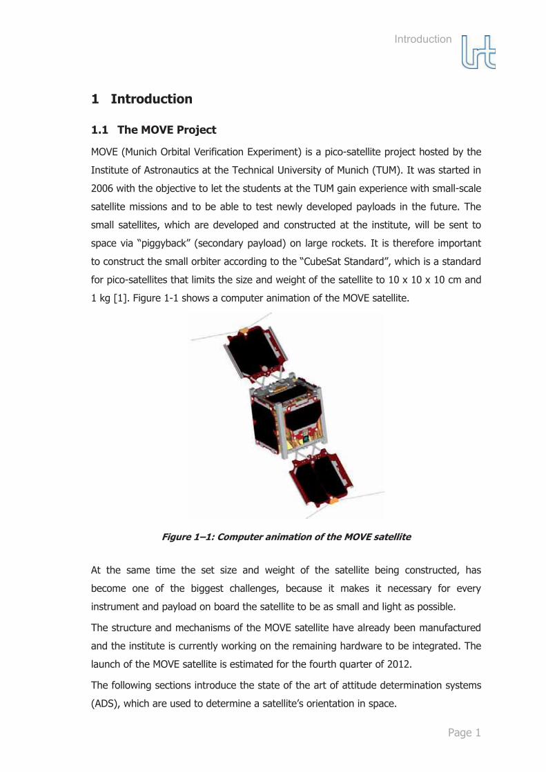
MOVE (Munich Orbital Verification Experiment) is a pico-satellite project hosted by the
Institute of Astronautics at the Technical University of Munich (TUM). It was started in
2006 with the objective to let the students at the TUM gain experience with small-scale
satellite missions and to be able to test newly developed payloads in the future. The
small satellites, which are developed and constructed at the institute, will be sent to
space via “piggyback” (secondary payload) on large rockets. It is therefore important
to construct the small orbiter according to the “CubeSat Standard”, which is a standard
for pico-satellites that limits the size and weight of the satellite to 10 x 10 x 10 cm and
1 kg [1]. Figure 1-1 shows a computer animation of the MOVE satellite.
Figure 1–1: Computer animation of the MOVE satellite
At the same time the set size and weight of the satellite being constructed, has
become one of the biggest challenges, because it makes it necessary for every
instrument and payload on board the satellite to be as small and light as possible.
The structure and mechanisms of the MOVE satellite have already been manufactured
and the institute is currently working on the remaining hardware to be integrated. The
launch of the MOVE satellite is estimated for the fourth quarter of 2012.
The following sections introduce the state of the art of attitude determination systems
(ADS), which are used to determine a satellite’s orientation in space.

Introduction
Page 2
1.2 Attitude Determination Systems: State of the Art
Since one of the objectives of the CubeSat constructed by the LRT is to fly scientific
and technical payloads, it is often important to know the spacecraft’s attitude. The goal
of an attitude determination system (ADS) is to determine the orientation (or attitude)
of a spacecraft relative to a known reference [2]. Figure 1-2 shows a satellite in orbit
around the Earth with its known body-fixed frame.
Figure 1–2: A satellite's body-fixed frame and the Earth's known reference frame [2]
An ADS is capable of determining the orientation of a satellite’s body-fixed frame with
respect to an external reference frame. This can be done, for example, by using the
sun, the local magnetic field direction or the stars as a reference. Each external
reference (e.g. a measured vector pointing in the direction of the sun) provides only
two of the three needed independent parameters (angular distance of the body-fixed
frame axes to the measured vector) to specify the spacecraft’s attitude [3] (page 355).
Like in figure 1-3, for a spacecraft in Earth orbit this can be done by the determination
of the local geocentric vertical coordinate system (LGCV), of which the z-axis is the
nadir, while the x- and y- axes are vectors pointing in the geographic directions (North,
South, East and West) of the geodetic datum (reference on Earth [4]) [5]. The nadir is
the downward-facing viewing geometry of the orbiting satellite and is equal to the
vertical direction that points in the direction of the force of gravity [6]. This again is
equal to the centripetal force of the satellite and therefore points in the direction of the
origin of the Earth’s frame. The abbreviation ECI in the coordinate system (figure 1-2)

Introduction
Page 3
stands for the use of the Earth-centered inertial coordinate system, which has its origin
in the geocenter [5]. Figure 1-3 shows the same satellite as in figure 1-2, but with the
LGCV reference coordinate system determined and computed by an ADS [2].
Figure 1–3: The satellite's LGCV coordinate system determined by an ADS [2]
The two frames (body-fixed frame and LGCV) enable the ADS to compute the satellite’s
orientation with respect to the determined reference frame (LGCV). One way to
compute the difference in orientation between the two frames is to calculate yaw, pitch
and roll of the satellite relative to the reference frame. These are the angles of rotation
in three dimensions about the spacecraft’s center of mass [7] (page 334). Figure 1-4
depicts this method. The red frames are body-fixed and the black frames are the LGCV
reference frames.

Introduction
Page 4
Figure 1–4: Yaw, pitch and roll angles of the satellite [2]
The purpose of an ADS can vary depending on the satellite mission. The most common
purposes are navigation feedback for satellites with active attitude control (change of
torque using actuators) and attitude information for the pointing of communication
antennas [2]. For remote sensing of the Earth’s atmosphere or surface, for example, it
is very useful to know the nadir of a satellite.
Active attitude control is especially important for satellites with a long lifespan. A space
vehicle is always subject to disturbance torques in space, as a result of gravity-gradient
effects, magnetic field torques, impingement by solar radiation, and, depending on
altitude, aerodynamic torques [3] (page 364). It can experience two kinds of different
disturbance torques: cyclic or secular. Cyclic torques vary as a sinus function during an
orbit, while secular torques accumulate with time and do not average out over an
orbit. Although these disturbances are mostly only in the range of around ,
they can over time cause the spacecraft to be reoriented. To prevent this from
happening most spacecraft use either magnetic property to passively stabilize along
the magnetic field or sense the disturbances using an ADS to actively apply corrective
torques [3] (page 354).
To determine the reference coordinate system of a spacecraft the ADS fuses data from
several different subsystems (sensors). The following sections are concerned with the
most common types of attitude determining sensors used for spacecraft. Generally, the
sensors are divided into two groups, the inertial- and the angle (or vector) sensors [2].

Introduction
Page 5
1.2.1 Inertial Sensors
Inertial (or rate) sensors determine the rate of rotation of the satellite in space. Two
types of inertial sensors will be introduced in the following sub-sections.
1.2.1.1 Gyroscopes
Gyroscopes (gyros) measure the speed or angle of rotation (rotation rate) around
various spacecraft axes with respect to an initial reference. No external reference
frame is used to accomplish attitude determination. Today different kinds of gyros are
available where the models range from simple spinning wheels, including iron gyros
using ball or gas bearings, to more accurate ring laser gyros. A non-laser gyro may
also be suspended using a set of gimbals, where the change in gimbal angles is
measured to determine the attitude-rate. This is based on the fact that the angular
momentum vector of a spinning body is constant in space [7] (page 371). Due to the
fact that gyros do not have an external reference (like the LGCV frame), they lack the
ability to provide absolute orientation information. One individual gyro can provide one
to two axes of information. To provide rotational rate information for all three axes,
several gyros are commonly grouped together into inertial reference units (IRU). To
finally obtain the spacecraft’s rotational position with respect to the initial reference the
measured rates have to be integrated over a period of time [7] (page 371). The
concept of a gyroscope enables very high bandwidth and extremely sensitive attitude-
rate information. As stated earlier though, they can only rely on one initial reference
frame, which naturally results in systematic errors in attitude determination over time
due to the effects of drift and inaccuracies of integration. These effects are also caused
by the mechanics of a gyro rotor, which cannot be maintained in truly torque-free
motion [7] (page 371). For this reason, it is common to add other sensors (as the ones
listed in section 1.2.2) to make up for the attitude determination errors by recalibrating
the gyro periodically. Models of high accuracy are mostly heavy and rather expensive
[7] (page 371). Figure 1-5 depicts one of NASA’s Gravity Probe B gyroscopes, which is
an ultra-precise gyro used to measure Albert Einstein’s hypothesized geodetic effect
[8]. It also shows a commercial ring-laser gyro, which measures differences in laser
interference patterns to determine rotation rates [2].

Introduction
Page 6
Figure 1–5: NASA’s Gravity Probe B gyro (coated gyro rotor and its housing)
(left) [8] and commercial ring laser gyro (right) [2]
1.2.1.2 Accelerometers
Accelerometers are used to determine the time rate of change of velocity of a
spacecraft. This is defined as the acceleration of the space vehicle [9]. There are
several different categories of acceleration sensors. An example is the use of the
piezoelectric effect, where microscopic crystal structures output a voltage relative to
their acceleration due to structural stress caused by the accelerative forces. Other
systems make use of the Hall effect by sensing the change in magnetic fields when
accelerated [9].
When an accelerometer is added to an inertial reference unit (IRU) for acceleration
sensing, the new unit is called inertial measurement unit (IMU) [3].
1.2.2 Angle/Vector Sensors
Angle (or vector) sensors use multiple angles (or vectors), which are directly measured
in the body-fixed frame, as reference vectors to determine the space vehicle’s
orientation [2]. The following five sub-sections present the most common sensors of
that kind.

Introduction
Page 7
1.2.2.1 Magnetometers
A magnetometer is an electromagnetic sensor that measures the ambient Earth’s
magnetic field direction and strength within the sensor’s fixed coordinates (body-fixed
coordinates). A complete measurement consists of three mutually orthogonal sub-
measurements of the magnetic field to create a three-dimensional vector space. The
three components then have to be compared with the known reference components of
the exact position of the satellite in orbit [7] (page 368). These reference components
are defined for each point in orbit around earth and are accessible using standard
magnetic field models like the International Geomagnetic Reference Field (IGRF) [2].
The most commonly used magnetic field models are based on the tilted-centered
dipole model, which is depicted in figure 1-6.
Figure 1–6: The tilted-centered dipole model of the Earth's magnetic field [10]
The spacecraft’s attitude can be derived from the difference between the measured
components in the body-fixed coordinates and the components taken from the
magnetic field model [7] (page 369). To be able to do this it is, as stated before,
necessary to know the exact position of the spacecraft. The two major drawbacks of a
magnetometer are therefore that the exact position of the satellite has to be known to
calculate attitude information and that even then only two out of the three rotation

Introduction
Page 8
angles can be measured at any one time (no angle information around the magnetic
field lines). Only after a full orbit can a three angle attitude be estimated as the local
magnetic field vector changes with respect to the LGCV frame over time. This does not
work for an equatorial orbit because the difference in frame orientation (over time)
changes as a function of latitude [2]. Figure 1-7 shows two different commercial
models of a magnetometer.
Figure 1–7: Two commercial models of a magnetometer [2]
1.2.2.2 Sun Sensors
Sun sensors use the Sun as an external reference. They measure one or two angles
between the body-fixed frame and the incident sunlight, while mostly using visible-light
detectors [3]. They can be designed to fulfill different tasks including initial orientation
acquisition, failure recovery of an attitude determination system or they could be part
of (a subsystem of) the normal attitude determination system. Satellites with a solar
array orientation system may use Sun sensors as a part of that system to allow for
pointing of the solar arrays [3]. They can either be used on spinning spacecraft, like
satellites with no or very limited attitude control, or on despun three-axis stable
vehicles [7]. Although hardware designs vary widely, they are all designed to either
provide digital or analog output signal formats [11]. Digital models mostly measure the
incident angle of the sunlight coming through the slit entrance in a plane perpendicular
to the slit [7] (page 365), which allows for the determination of one angle with a
discrete output. To obtain a vector within the body-fixed frame pointing at the Sun,
two Sun sensors are mounted orthogonally on each side of the space vehicle. Digital
Sun sensors have a resolution measured in binary bits. The digital sensor in figure 1-8
below has a resolution of four bits as a result of the four separate detector elements.

Introduction
Page 9
Figure 1–8: Digital Sun sensor with sensor output voltage and signal [11]
An analog Sun sensor outputs a continuous function of the angle of incidence [11].
Figure 1-9 depicts an analog sensor with two separate photosensitive elements. The
difference in the current outputs of the two elements is measured and translated into
the incident angle. If the difference is zero, the null point of the sensor is reached [11].
An aperture plate could also be used instead of the lens.
Figure 1–9: Analog Sun sensor with output voltage [11]
It lies in the nature of a Sun sensor that an unobstructed field of view (FOV) to the
Sun is necessary. It can under certain circumstances be a challenge to provide for the
clear view of the Sun sensor, especially when the spacecraft has a lot of external
components. In addition to that most orbits around Earth (especially low-Earth orbits)
include eclipse periods when the Sun is not in the FOV of the space vehicle. This loss
of orientation data has to be compensated for by other sensors to maintain attitude
determination [3] (page 371).

Introduction
Page 10
1.2.2.3 Horizon scanners
Horizon scanners have the ability to define the position of the horizon on each side of a
spacecraft in an orbit around Earth, which enables a computer system to precisely
define the nadir point. This method is especially reasonable for space vehicles in LEO
(low-Earth orbit), where the cone angle of the Earth, which depicts the spacecraft’s
view of the Earth, will always be greater than 120° [7] (page 367). Most horizon
scanner models are infrared devices that detect the contrast between the cold of deep
space and the heat radiation of the Earth’s upper atmosphere [3] (page 375). They
make use of the atmosphere’s band, which radiates infrared light (15 μm
wavelength) day and night and is, because of its thin layer, well defined in altitude. Its
radiation is also not affected by clouds. These characteristics make the band a
reliable reference for attitude determination. Models range from rather simple narrow
FOV fixed-head types (also known as pippers/horizon crossing indicators) to the more
complicated scanning horizon sensors. Pippers are used on spinning spacecraft and
measure Earth phases as a rising pulse and falling pulse as the pipper encounters
going from cold space across the Earth and back into cold space [7]. Along with orbit
and mounting geometry information several sensors are able to define the pitch and
roll angle relative to the nadir [3]. Scanning horizon sensors use a rotating mirror or
lens to augment the spinning of the spacecraft [3]. The difference between the
expected pulse (relative to the orientation of the mirror) and the actual occurring pulse
gives information about the pitch angle. By using another sensor mounted
orthogonally, roll information will also be available (see figure 1-4). It is not possible to
determine yaw information using horizon scanners, because the Earth always appears
circular to the spacecraft for every given yaw angle [7]. Figure 1-10 shows the concept
of a scanning horizon sensor [12].

Introduction
Page 11
Figure 1–10: Concept of a scanning horizon sensor [12]
The main drawback of a horizon scanner is the variation in altitude of the band. It
can vary by as much as 20 km from point to point on the Earth’s surface and is
affected by different times of the day and year as well. For spacecraft orbiting in LEO
this limits accuracy to around 0.05° (unless taking into account the Earth’s oblateness)
[7].
1.2.2.4 Star Sensors
Star sensors are generally used for missions with the need of very high-accuracy
attitude determination. Two types of star sensors are available, which are both based
on image processing: star scanners for spinning spacecraft and star trackers for three-
axes stabilized spacecraft. Scanners are restricted in their FOV by multiple slits. The
attitude of the space vehicle can be derived from several star crossings (as seen
through the slits by the scanner) [3] (page 374). Trackers on the other hand track
fixed stars to derive attitude information. Some systems even identify the viewed star
pattern to obtain orientation information [3]. Unlike the other sensors of this section,
star sensors do not experience major constraints in accuracy but rather in the system
itself. Star sensors are generally sensitive to bright light and could already be blinded
by the light coming from other planets, not to mention the sun. This has to be kept in
mind when integrating these heavy and costly units. Another operational problem is
caused by the time gaps between star identification (and orientation). They can be up
to half an hour long, depending on the amount of star sensors used and the

Introduction
Page 12
spacecraft’s orbit [7]. For this reason star sensors are often combined with gyroscopes
(see section 1.2.1.1) to provide for the high-accuracy (but low frequency) external
reference that the gyroscopes lack [3]. Figure 1-11 shows a model of a star tracker by
Ball Aerospace and Technologies Corp. [13].
Figure 1–11: Star tracker by Ball Aerospace and Technologies Corp. [13]
1.2.2.5 Global Positioning System (GPS)
To determine orientation information for all three axes using GPS signals, it is
necessary to have at least three antennas mounted at different points on the
spacecraft. The relative position of the three antennas in the Earth-centered frame is
determined by resolving small phase differences of the wavelengths transmitted by
satellites in high Earth orbit. Although this concept is a relatively economic (in terms of
cost, power, size and weight) it does require the spacecraft to have a reasonably large
baseline, which often poses a limit of accuracy. Multipath effects due to reflections off
vehicle components can add to the inaccuracy. Until now, they are mostly used in low-
accuracy applications or as back-up sensors. [3,7]
All sensor data (section 1.2.1 to 1.2.2) that was taken from source [3] can be found on
page 371-375.
1.2.3 Summary
For a direct comparison of the various sensor models, it is important to find the most
vital parameters that have an impact on the mission requirements. Typically ADS
subsystems have the most direct impact on the overall requirements in their size,

Introduction
Page 13
weight, power supply and accuracy. Another determining factor for the sensor
selection is the application of the spacecraft. Table 1-1 briefly summarizes all sensor
data of this chapter with respect to the given parameters, excluding size because of its
great variability.
Table 1-1: ADCS sensors and their typical properties [2,3]
Sensor type Typical
accuracy
(degrees)
Weight
range
(kg)
Power
consumption
(W)
Application
Horizon
sensor
0.02 – 1.0 0.5 – 4.0 0.3 -10.0 Earth orbiters
(spinner or
three axis
stabilized)
Magnetometer 0.5 – 3.0 <1.0 <1.0 Earth orbiters
(three axis)
Sun sensor 0.005 – 3.0 < 0.5 0 – 3.0 Solar cell
pointing, Sun
vector
determination
Star sensor 0.0002 –
0.08
2.0 – 5.0 5.0 – 20.0 High precision
pointing
Inertial
Measurement
Unit
Gyro drift
rate: 0.003
deg/hr – 1
deg/hr, acc.
1.0 – 15.0 10.0 – 200.0 High
frequency
inertial
determination
1.3 Current Attitude Determination Systems for MOVE
As introduced in section 1.1, MOVE is a CubeSat in development at the Institute of
Astronautics at the Technical University of Munich. Its current ADS consists of only a

Introduction
Page 14
Sun sensor subsystem, which uses four separate two-axes analog Sun sensors on each
side of the cube to determine a reference (Sun) vector. It was developed and
manufactured by the University of Denmark (DTU) and was later adapted for MOVE by
Thomas Bickel (a TUM student) who designed a circuit board for the integration of the
sensor at the Institute in Munich. Although the system does not include active attitude
control of the satellite, it does use a passive configuration to correct disturbance
torques and to align the satellite with the Earth’s magnetic field. To achieve this, a
permanent magnet and hysteresis rods are built into the satellite’s structure [14].
While the permanent magnet aligns the satellite depending on the surrounding flux
lines, the hysteresis rods dampen the effects of variations of the magnetic field by
upholding (only over a certain time span) a magnetized state equal to the ambient
magnetic field before the variation [15]. This procedure weakens the effect of the
variation on the permanent magnet and therefore stabilizes the satellite in space.
The Sun sensor itself uses two pairs of rectangular photodiodes mounted perpendicular
to each other. In figure 1-12 they are depicted as L (left) with R (right) and T (top)
with B (bottom). The two diodes of one pair are separated by a small space between
them. The abbreviation REF stands for the two reference diodes. The optical slit in the
aperture plate is respectively parallel to the space between the diodes [16].
Figure 1–12: Pairs of diodes on the DTU sensor
Depending on the incident Sun angle, one of the two diodes of one pair will output a
greater current than the other, which is partially covered by a shadow of the aperture
plate. The two normalized quotients
and (1-1)

Introduction
Page 15
allow for independence of intensity and give direct information about the angles
against the Sun vector in the body-fixed frame.
Its size measures only 14 x 22 mm. Figure 1-13 left shows the Sun sensor without its
circuit board mounting compared to a pencil and the right image depicts the size
constraints and the layout of the sensor mounted on its circuit board [16].
Figure 1–13: DTU Sun sensor size compared to pencil (left) and size constraints of the DTU Sun sensor [16]
The sensor’s main advantages are its small size, low power consumption and its high
accuracy, which is specified to ±1°. Nevertheless the sensor’s layout is connected to a
crucial disadvantage, which is related to the sensor’s mounting. The set-up uses
extremely fragile wire bonds (see figure 1-14) to connect the diodes with the circuit
board. During the course of the MOVE project two of the four available sensors were
already severely damaged and cannot be used any longer. The remaining two reliably
working sensors will not cover complete attitude determination for the satellite and
there are no more of these unique sensors available to acquire.
Figure 1–14: DTU Sun sensor connected to PCB via fragile wire bonds [16]

Introduction
Page 16
1.4 Statement of Work (Scope)
The circumstances described in section 1.3 were the initial reason for the development
of a follow-up sensor for MOVE to replace the damaged system. They underline the
urging necessity of a new attitude determination system for the project. The
requirements imposed on a new system are to stay as close as possible to the
structural set-up and properties of the DTU sensor and to deliver similar precision
rates. An ADS is necessary for the MOVE satellite to enable analysis of its change in
orientation over time and to evaluate newly developed solar cells, flown as
experimental payload on the satellite. To be able to do this it is necessary to know the
spacecraft’s relative orientation to the Sun during experimentation. Another reason for
the development of a follow-up sensor system is to support analyzing images taken
from the onboard camera of the satellite.

Design and Construction of the PSD-based Sun Sensor Prototype
Page 17
2 Design and Construction of the PSD-based Sun Sensor Prototype
2.1 Requirements and Goals
The two specifications of an ADS that are most directly affected by the mission
requirements are the spacecraft’s required orientation and accuracy in determining that
orientation. A satellite designed for Earth remote sensing would, for instance, require
its ADS to deliver accurate Earth-pointing (nadir-pointing) for it to analyze the Earth’s
topography. Other determining factors that play an important role in the choice of a
compatible ADS are the mission’s specified fault tolerance, FOV requirements, available
data rates and its redundancy [3] (page 375). Every mission has its own purpose and
functionality, from which the requirements for its supportive sub-systems can be
derived.
The purpose of the MOVE CubeSat is mainly to provide university students with hands-
on experience in satellite engineering. Its secondary goal is to collect scientific data
measured in space. On its way to space it will carry four newly developed high-
efficiency solar cells, which were designed and constructed by AZUR SPACE Solar
Power GmbH and provided to TUM by EADS Astrium. The 40 x 80 mm triple-junction
solar cells have an efficiency of 30% and are of the type TJ Solar Cell 3G30C [17].
They will be tested as a part of the satellite’s operations and later evaluated on the
ground. The four cells are mounted on different sides of the cube and take up half the
space of the side area each.
An accurate evaluation of the solar cells requires the satellite to have Sun vector
coordinates available within its body-fixed frame, because they are vital for analyzing
the cells’ efficiency depending on the incident angle of the sunlight. In addition to that
a suitable ADS should be able to perform initial attitude acquisition using an external
reference. This is especially important because the satellite is ejected randomly from
the carrier rocket. An external reference will provide reliable inertial pointing for the
spinning body in space. As mentioned earlier, MOVE does not include an active attitude
control system and therefore does not rely on high precision attitude determination,
which is needed for the use of actuators. It is purely of scientific interest to obtain
information about the satellite’s spinning behavior in space.
Beside the accuracy and functionality requirements of the ADS, aspects of suitable
integration are just as decisive. Since the goal is to replace an existing system, it will

Design and Construction of the PSD-based Sun Sensor Prototype
Page 18
be useful to adopt as many specifications as possible for a new sensor. This primarily
implies staying within the size, weight, power and FOV constraints of the current
system (section 1.3), while meeting all accuracy and functionality requirements
imposed on the ADS by the mission itself.
The weight of the current system of 120 mg (excluding package and electronics) and
its size of only 7 x 8 mm (14 x 22 mm including circuit board) are crucial constraints
that have to be kept in mind when designing a new sensor system. For the third
dimension of size, the MOVE structural configuration of the satellite allows up to 6 mm.
Further, the current sensors use a FOV of 140° and only require power for
communication components (all together: 9.48 mW) to deliver orientation information.
Their allowed specified operating temperature ranges from -30 to +80 °C. To
efficiently make use of existing communication software, it is reasonable to aim for the
use of the same communication interface as it is used for the current system, which is
based on Serial Peripheral Interface (SPI) communication. All these properties and the
goal of achieving a similar specified accuracy (1° specified for the DTU sensor) are
determining factors and requirements imposed on the design of a new sensor system
[18]. The strict requirements of the sub-system are simultaneously closely related to
the CubeSat specifications.
The final goal of the work described in this paper is to construct, characterize and test
a new sensor system for the MOVE satellite and to later compare its properties with
pre-developed systems. Figure 2-1 visually summarizes all mentioned determining
factors for the design of a future sensor system for MOVE.

Design and Construction of the PSD-based Sun Sensor Prototype
Page 19
Figure 2–1: Determining factors of the requirements and constraints for a new sensor system for MOVE
2.2 Sensor Selection Process
To be able to determine the best, most cost-effective approach in sensor selection, a
trade study was conducted. Referring back to section 2.1, it was defined as most
important that the follow- up sensor is capable of providing inertial pointing for initial
attitude acquisition and Sun vector pointing. (see figure 2-1) Table 2-1 correlates the
different sensor types with their met MOVE requirements.
Requirements for a new
sensor system for MOVE
inertial pointing for
initial attitude acquisition
Sun vector pointing for experimental
payload evaluation
max. sensor size of 14 x 22 x 6 mm
max. sensor
weight of
~120 mg
goal: accuracy of <1°
field of view use of 140° Thermal
requirement: operation
from -30 to +80 °C
power constraints:
≈10 mW
SPI communica
tion interface
No active attitude
control of the satellite

Design and Construction of the PSD-based Sun Sensor Prototype
Page 20
Table 2-1: Sensor types and their fulfilled (��) MOVE requirements
MOVE requirements Horizon
sensor
Magnet
ometer
Sun
sensor
Star
sensor
IMU
Inertial pointing � � � � �
Initial acquisition � � �
Sun vector pointing �
Max. size: 14x22x6 mm � �
Max. weight: 120 mg �
Accuracy goal: <1° � � � �
Thermal specifications � � � � �
Power: <10 mW � �
Taken from table 2-1, the only sensor that fulfills initial acquisition and Sun vector
pointing criteria is the Sun sensor. While the horizon- and star sensor can be used for
initial acquisition (due to the use of an external reference), both the magnetometer
and the IMU require external periodic recalibration to determine the attitude. The only
reasonable solution for Sun vector pointing is the use of a Sun sensor, which directly
determines the vector via external (Sun) reference. Therefore the sensor that best
supports the main functionalities and goals of the mission is the Sun sensor.
The second step is then to examine whether the chosen sensor, which already fulfills
all main criteria, complies with all other implementation requirements such as size,
weight and thermal constraints. Table 2-1 shows checks for the Sun sensor for all
secondary MOVE requirements. Nevertheless it has to be kept in mind that the Sun
sensor has drawbacks in inertial pointing as well: it does not function during eclipse.
While this heavily affects attitude determination, it does not have any effect on the

Design and Construction of the PSD-based Sun Sensor Prototype
Page 21
ability to evaluate the solar cells, because they also rely on sunlight to generate power.
The most effective way to avoid loss of attitude determination during eclipse is to
combine several sensors (e.g. Sun sensor and magnetometer), but since the goal of
this project is to develop one follow-up sensor to replace the current model, this would
be part of successive work. It was finally decided to develop a Sun sensor because it
fulfills all mission criteria when the satellite is not in eclipse and there was no
requirement to do so during the eclipse phases.
2.2.1 Available Sun Sensor Types
As stated in section 1.2.2.2, there are generally two different types of Sun sensors:
analog and digital models. Various commercial aerospace companies offer Sun sensors
to be acquired on the global market. These include the Adcole Corp., Ball Aerospace
and Technologies Corp., EDO (Barnes) Corp., Ithaco Space Systems Inc., and
Lockheed Martin [3]. Offers range from highly-sophisticated heavy-weight digital
sensors to simple analog sensors, but none of the models are designed specifically for
CubeSats and therefore do not meet the vital requirements regarding size, mass and
power consumption. Other companies, like Clyde Space, provide entire modules for
attitude determination and control especially for CubeSats, but do not offer single
sensors that meet the MOVE requirements. One example of a single sensor offered by
the ISIS CubeSat online shop is their “Miniaturised Analog Fine Sun Sensor,” which
meets all but the mass and size requirements. It weighs 50 g and its total size is 46 x
45 x 14 mm [19]. Hence, to best suit the needs of the MOVE mission, it was necessary
to design a new sensor that is capable of using the current infrastructure designed for
the DTU Sun sensor and fulfills all specified criteria.
Another approach, apart from developing a new system, is to test current components
of the satellite itself on their ability to determine attitude. The only existing satellite
component with attitude determination potential is a solar cell. Since any solar cell’s
output is dependent on the light’s incidence angle, MOVE’s experimental payload
3G30C features an opportunity to calculate this angle. This is based on the idea that
the heat flux density, meaning the radiated energy per area and time on a solar cell, is
directly dependent on the radiation’s incidence angle [20]. The connection is expressed
in the formula:
, (2-1)

Design and Construction of the PSD-based Sun Sensor Prototype
Page 22
where is the actual radiant flux (radiant power) and is the radiant flux for an
incidence angle (θ) of 90° (perpendicular to the cell’s surface) [20]. The cell’s ability to
determine θ knowing and with
, (2-2)
will, as explained later, be tested and evaluated along with a newly developed sensor
system as it is introduced in the following.
2.2.2 Sensor Principle Solution for Development
In a coordinate system two points are needed to define a distinct vector. For the Sun
sensor this means that a way to obtain the Sun vector is to determine two different
points in body-fixed coordinates along the Sun’s light beams (these can be considered
parallel in Earth orbit due to the large distance between Earth and the Sun). To be able
to do this with a changing incident angle of the light, one of the two determined points
has to be variable depending on the angle. This can be achieved by using an aperture
plate to extract only a fine beam with the hole defined as the fixed point, which the
beam passes through. This principle is shown in figure 2-2.
Figure 2–2: Sun sensor principle with aperture plate
The body-fixed coordinates of the point P and the hole (defined as point Q) in the
aperture plate define the distinct Sun vector. In three dimensions the vector can be
expressed as

Design and Construction of the PSD-based Sun Sensor Prototype
Page 23
, (2-3)
where the origin of the coordinate system is point Q (the hole), positive x goes to the
right, positive y comes out of the paper plane, and positive z goes upwards. Point P
changes with respect to the change in incident angle θ. Therefore one exact incidence
angle is defined for every value of P.
To be able to determine point P in the coordinate system it was necessary to find a
suitable instrument that can read out the exact position of the light spot in two
dimensions. Section 2.3 introduces the Hamamatsu PSD, which was selected to fulfill
this purpose.
2.3 The Hamamatsu Position Sensitive Detector
The Position Sensitive Detector (PSD) is an optical device offered for sale by the
Japanese company Hamamatsu Photonics. Generally there are two kinds of different
PSD types: one- and two dimensional detectors. The first kind merely determines the
light spot position in one direction (e.g. x-axis) while the two dimensional device
outputs information in two directions (x- and y-axis). To match the criteria stated in
section 2.2, the two dimensional model was acquired, which will, combined with an
aperture plate, allow for full three axis Sun vector determination. The PSD is normally
used for the purpose of laser beam alignment or object tracking such as monitoring
eye movement [21]. It was nevertheless chosen for this project, because it facilitates
the required unique light spot determination traits. Figure 2-3 shows the two available
PSD sizes (4 x 4 mm and 9 x 9 mm active areas).
Figure 2–3: The Hamamatsu PSD (4 x 4 mm and 9 x 9 mm active areas) [21]

Design and Construction of the PSD-based Sun Sensor Prototype
Page 24
2.3.1 PSD Specifications
The two different PSD sizes shown in figure 2-3 are nearly identical in their
specifications. To be able to work with and test the device, the larger version of the
type S5991-01 was chosen. The reason for that is the fact that this paper primarily
focuses on the proof of concept of the new system, where large components alleviate
the process of troubleshooting and mechanical handling. For integration purposes
(especially because of the smaller size and weight) all following set-up steps can be
translated for application on the smaller version (type S5990-01), but are not carried
out within this project. All following data and specifications on type S5991-01 were
taken from the official data sheet provided by Hamamatsu [21].
Version S5990-01 measures only 8.8 (±0.15) x 10.6 (±0.2) x 1.26 (±0.15) mm (active
area 4 x 4 mm) and is therefore well within the specified size constraints (see section
2.1). The PSD unit that is used for this project (sensor development) measures 14.5
(±0.2) x 16.5 (±0.2) x 1.26 (±0.15) mm and has an active area of 9 x 9 mm. The
active area consists of a photosensitive surface to which four anodes are connected
(see figure 2-4: X1, X2, Y1, Y2). The detector makes use of the photovoltaic effect.
Depending on the position of the light spot on the active area, the four anodes
measure different current values. With the recommended spot light size of 0.2 mm in
diameter, the position detection error is typically in the range of only ±150 μm, while it
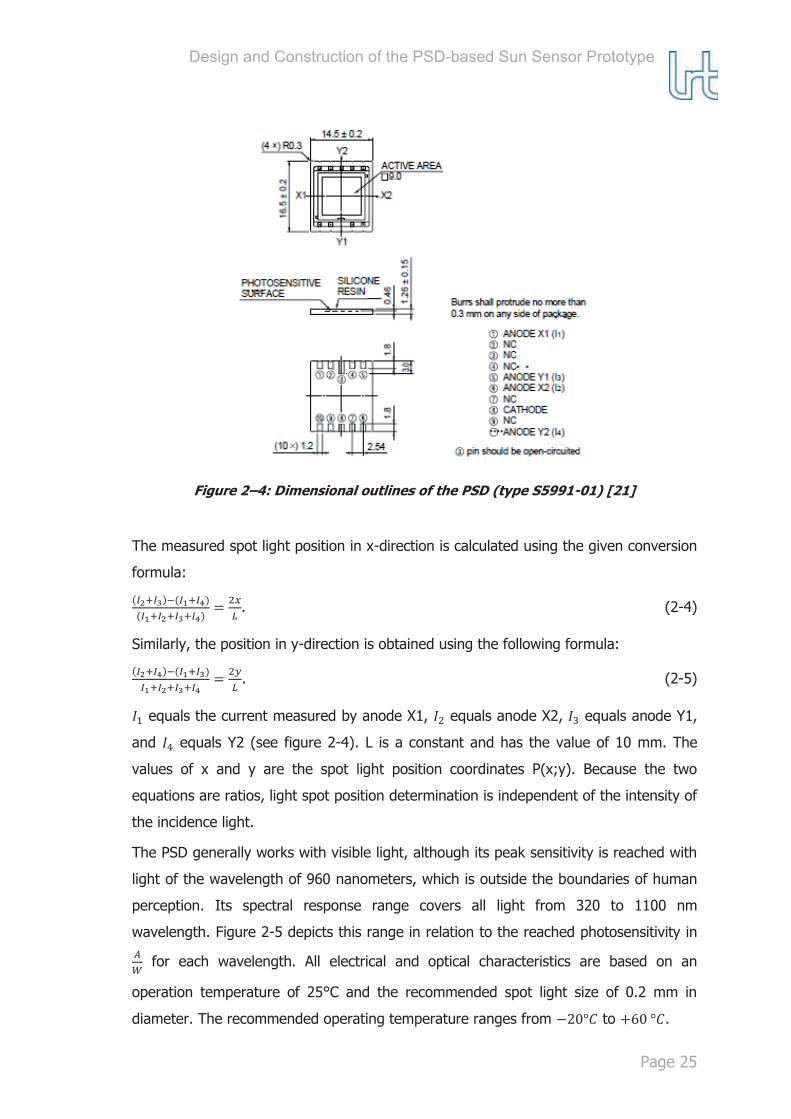
has a position resolution of 1.5 μm. Figure 2-4 depicts the PSD’s dimensional outlines
(type S5991-01).
Design and Construction of the PSD-based Sun Sensor Prototype
Page 25
Figure 2–4: Dimensional outlines of the PSD (type S5991-01) [21]
The measured spot light position in x-direction is calculated using the given conversion
formula:
. (2-4)
Similarly, the position in y-direction is obtained using the following formula:
. (2-5)
equals the current measured by anode X1, equals anode X2, equals anode Y1,
and equals Y2 (see figure 2-4). L is a constant and has the value of 10 mm. The
values of x and y are the spot light position coordinates P(x;y). Because the two
equations are ratios, light spot position determination is independent of the intensity of
the incidence light.
The PSD generally works with visible light, although its peak sensitivity is reached with
light of the wavelength of 960 nanometers, which is outside the boundaries of human
perception. Its spectral response range covers all light from 320 to 1100 nm
wavelength. Figure 2-5 depicts this range in relation to the reached photosensitivity in
for each wavelength. All electrical and optical characteristics are based on an
operation temperature of 25°C and the recommended spot light size of 0.2 mm in
diameter. The recommended operating temperature ranges from to .

Design and Construction of the PSD-based Sun Sensor Prototype
Page 26
Figure 2–5: The PSD spectral response range [21]
The PSD can produce a saturation photocurrent of 500 μA (under the condition of a
reference voltage of 5 V, using a 1 kΩ resistor and a 900 nm wavelength light beam),
which is the maximum electric current light can evoke on the PSD.
To identify whether the PSD qualifies for application on the MOVE satellite, all its
specifications have to be compared with the requirements imposed on the system.
Table 2-2 matches the above mentioned data with the MOVE requirements of section
2.1.
0
0,1
0,2
0,3
0,4
0,5
0,6
0,7
0 200 400 600 800 1000 1200
phot
osen
siti
vity
(A/W
)
wavelength (nm)
PSD spectral response
PSD spectral
response

Design and Construction of the PSD-based Sun Sensor Prototype
Page 27
Table 2-2: PSD characteristics at 25°C (spot light size 0.2 mm) [21] and the MOVE requirements
Parameter PSD S5991-01
(typical values)
MOVE Requirements
Spectral response
range
320 to 1100 nm none �
Position resolution 1.5 μm (I=1 μA; f=1
kHz)
Sensor to be tested for 1°
accuracy
Saturation
photocurrent
500 μA ( ;
λ ; Ω)
none �
Operating
temperature
-20 to +60 °C To be tested in thermal-
vacuum chamber
�
Communication SPI interface possible SPI interface �
Power Only for
communication, same
as the DTU sensor
9.48 mW for SPI
communication
�
Weight To be measured with
S5990-01
120 mg sensor
Size 14.5 x 16.5 x 1.26 mm 14 x 22 x 6 mm * �
The PSD has to be thoroughly tested whether it meets all of the in section 2.1 defined
requirements of an ADS for MOVE, particularly with regard to its thermal specifications.
Since there is no official thermal constraint for sensors on the MOVE satellite yet, the
* This requirement is met by type S5990-01

Design and Construction of the PSD-based Sun Sensor Prototype
Page 28
current Sun sensor’s thermal specifications (see figure 2-1) were taken as a reference.
Because they are not fulfilled by the PSD, this aspect has to be analyzed in detail as
part of the successive work. An option for expanding the operating temperature range
if necessary is the use of the existing heaters for active thermal control.
The approximate 0.3 PSD volume makes up around 0.03 per cent of the 1000
the entire CubeSat measures. This does not include multiple sensors to cover all four
sides of the satellite and the sensors’ circuit boards. Whether the desired accuracy of
the system, which is up to 1°, can be achieved with the precise position resolution of
1.5 μm over the 81 active area will be tested in the course of this paper. All in all,
the PSD qualifies in its main specifications for use on a CubeSat.
2.3.2 The Test Circuit Board for the PSD
To mechanically support and to electrically connect the PSD with other components
used for communication it was necessary to design a suitable printed circuit board
(PCB). PCBs use conductive pathways, which are etched from copper sheets laminated
onto a nonconductive substrate [22], to supply power and to transfer data (in form of
electric signals) from component to component. Since the PSD is predestined to use
the same devices for communication as the DTU Sun sensor does (which are already
installed on the CubeSat), these devices have to be installed on the test PCB as well.
As this PCB is merely for testing, and not intended to function as a flight model, size
constraints are not met for handling purposes. The following sub-sections give an
overview of the three components needed for communication.
2.3.2.1 Operational Amplifier AD8554
Because the actual currents at the four anodes generated by the PSD are too small to
be measured directly (max. 500 μA), a transimpedance amplifier is used to convert the
current to a voltage, which is then amplified. As an operational amplifier (op-amp) the
component AD8554 is part of the transimpedance amplifier circuit. This basic circuit is
shown in figure 2-6. The resistor R is 680 kΩ., which yields and output voltage of up to
2.5 V. The AD8554 is a high precision, rail-to-rail op-amp and consists of a main and a
secondary amplifier. It operates from 2.7 to 5 V with a single supply and withstands
temperatures from -40 to +125 °C, which is within the specified range (see section
2.1). [23]

Design and Construction of the PSD-based Sun Sensor Prototype
Page 29
Figure 2–6: Transimpedance amplifier circuit [24]
2.3.2.2 Voltage Reference AD1582
The Analog Devices AD1582 is a low power, low dropout, precision band gap reference
of 2.5 V. It is, just like the AD8554, specified to operate from -40 to +125 °C. The
device has a low supply voltage headroom of voltages as low as 200 mV above the
output voltage (2.5 V) [25]. It is needed to produce a reliably constant voltage
irrespective of power supply variations or its loading. This voltage is used as a
reference for measuring the voltage that is output by the transimpedance amplifier.
2.3.2.3 Microchip MCP3004
The Microchip MCP3004 is used on the PCB to convert the analog voltage comparison
of AD8554 and AD1582 for all four channels into digital 10 bit values (A/D conversion).
It has an SPI (Serial Peripheral Interface) bus to communicate with a central
processing unit (CPU). The device operates with a voltage supply between 2.7 and 5.5
V and is specified to work within a temperature range of -40 to +85 °C [26]. It
communicates with a CPU in a master-slave-relationship, where the MCP3004 is the
slave component, and is connected to the CPU via four communication channels: Serial
Clock (CLK), Serial Data Out (DOUT), Serial Data In (DIN), and Chip Select (CS). In
addition it is connected to a +3.3 V power source and the ground (GND).
Figure 2-7 depicts all component connections on the PCB and its in- and output
channels. All parts marked with a C are 100 nF capacitors, while the title R represents
a 100 kΩ resistor. The connection diagram can be seen in the appendix section A2.

Design and Construction of the PSD-based Sun Sensor Prototype
Page 30
Figure 2–7: TARGET PSD PCB layout
The final PCB with the PSD integrated is shown in figure 2-8. It is the same PCB as
seen in figure 2-7. All components apart from the PSD are mounted on the back side.
Figure 2–8: Final PCB for the PSD
2.3.3 The Aperture Plate
The sensor principle explained in section 2.2 works only with a fitting aperture plate
that isolates a fine sunlight beam (see figure 2-2). The aperture plate designed for the
PSD circuit board is a simple piece of bent sheet metal that is kept in place by spacers.
To avoid light distractions on the PSD, the aperture plate has to be able to block the
entire photosensitive surface from exposure to light other than light that passes
through the hole. The hole itself is 0.2 (±0.05) mm in diameter and was drilled into a

Design and Construction of the PSD-based Sun Sensor Prototype
Page 31
thin (0.1 mm) plate to minimize light reflection off the edges of the hole. The size
decision is based on the recommendation for spot light size in the Hamamatsu data
sheet [21], which is also 0.2 mm. Because of the small distance between the aperture
plate and the PSD in relation to the hole size, diffraction phenomena of the light beam
can be neglected.
Figure 2–9: The aperture plate for the PSD
The distance between the PSD’s active area and the hole (h) in the aperture plate
defines the minimum incidence angle, for which the PSD detects light. The greater h
becomes the smaller the field of view (FOV) of the sensor. The FOV (α) depending on
h can be expressed using the following equation:
. (2-6)
Because PSD’s active area has the form of a square with a side length of 9 mm, light
spots in the corners will entail a greater FOV, while light spots at the edge half way
across the sides yield the α FOV (in degrees) expressed by equation (2-6). Exemplary,
for h = 5 mm the FOV angle is roughly 84°. To achieve a FOV of 140° (α=140) as it is
specified in section 2.1, h has to be as small as 1.64 mm. With this assembly, the Sun
vector can be obtained for any incidence angle within the specified FOV using formula
(2-3), where equals the magnitude of h.

Sensor Verification Method
Page 32
3 Sensor Verification Method
3.1 Evaluation Process
All in all, three different sensor systems will be tested and compared in their
performance. These include the current DTU Sun sensor (see section 1.3), the PSD-
based Sun sensor (see section 2.3), and the experimental solar cell payload (see
section 2.2.1). When testing, all three methods are evaluated under the same
circumstances, so an accurate conclusion on which type qualifies and substitutes the
DTU sensor best, can be drawn. The following sections introduce the methods and
materials utilized for sensor validation.
3.2 Simulation of Satellite Orientation Positions in Space
As stated in section 1.3 the MOVE satellite does not have an active attitude control
system. It merely relies on its passive system to align it along the Earth’s magnetic
field lines. In addition to that it is randomly ejected from its launch vehicle into orbit,
which does not allow for initial information about rotational behavior. In this situation,
the Sun sensor can be used to acquire attitude information. To be able to rely on the
sensor’s ability to perform this function in space, it has to be thoroughly tested on
Earth before launch. The simplest way to do this is to simulate possible satellite
orientations relative to the Sun (light source), which are then compared to the sensor’s
output data. This also allows for specification of the accuracy of the sensor.
For this purpose, a motor setup, which was developed by the Institute of Astronautics
at the Technical University of Munich, was used. It was originally built for the
Lightweight Intersatellite-Antenna (LISA) project. The LISA motor setup is capable of
rotating a platform around two axes, which simulates two of the three possible satellite
rotations around pitch, roll and yaw. For antennas, rotation equal to compass bearing
change is called azimuth, while the elevation angle reflects the attitude of an observed
object [27]. (Note: these definitions are used because the motor is usually utilized to
point the LISA antenna) Figure 3-1 shows the LISA motor setup with its axes.

Sensor Verification Method
Page 33
Figure 3–1: LISA motor setup with its two axes for rotation
The rectangular platform (middle) with mounting bolts (left) and the circular interface
(right) were specially designed with the CAD (computer-aided design) software CATIA
(by Dassault Systèmes) to fit the mounting needs of the PSD sensor’s PCB (see section
2.3.2). The parts are shown in figure 3-2.
Figure 3–2: Sensor mounting parts (CATIA screenshots)

Sensor Verification Method
Page 34
LabView Motor Control
As mentioned before, the LISA motor will simulate different satellite orientation
positions for the sensors. To do this, it has to be programmed to run a certain
sequence. The motor is controlled via Trinamic Motion and Interface Controller, which
has an RS232 interface. This interface is included in a National Instruments PXI (PCI
Extensions for Instrumentation), which is a PC-based platform for measurement and
automation systems. It is used as an electrical bus for interconnection of peripheral
components (PCI) such as the LISA motor and is controlled through an external PC.
Systems are developed using the National Instruments LabVIEW software. This setup
is shown in figure 3-6.
The motor sequence is divided into seven parts; one for every 15° of azimuth change.
For each azimuth position, the motor rotates the platform with the sensor by 180°
around the elevation axis (90° in both directions). This covers every position, from
which the sensor can detect light from a fixed light source, which resembles the sun.
The 15° steps are used to evaluate the sensors’ performance for different azimuth
angles (different alignment with respect to the light source).
Figure 3-4 shows how this is implemented as a computer program or virtual instrument
(VI) in LabVIEW. The following description requires a basic understanding of the
LabVIEW graphical programming language. It is beyond the scope of this paper to
include an introduction to this language, the reader may refer to the National
Instruments Homepage (http://www.ni.com) for further information. All following
numbers in parentheses represent positions on figure 3-4.
There are two variables that represent the setpoints to which the motors are
commanded. These are initialized with 0° for azimuth and -90° for elevation (1). The
values are written to two global variables (2) to send their information via another VI
to the motor, which starts turning into the demanded position. To leave time for the
turning process before giving new commands, the while loop (3) only stops, when both
the commanded azimuth, and elevation position is reached. This is done by comparing
two global variables for both axes: “Stellwert” (setpoint) and “Position”. “Stellwert”
holds the value of the position command, while “Position” gives the current position of
the motor. One of each variable is used for every axis (4). The stop signal for loop (3)
is therefore only given, when the two variables are equal for both axes and the motor

Sensor Verification Method
Page 35
has reached its position. After the first loop iteration of the outer while-loop (5) this
position is 0° azimuth and 90° elevation. The sensor will have recorded data during
this first part of the sequence. In order to start the second part, the azimuth motor has
to turn the sensor by 15°, while the elevation motor goes back to -90°, so it can turn
the sensor around 180° during the following loop iteration. As a result, the “Elevation
Stellwert” is negated after every loop iteration of (5), while the “Azimuth Stellwert” is
only increased by 15° every second loop iteration. This is controlled by a case
structure, for which a Boolean constant is inverted every loop iteration. The entire
process is stopped after 13 loop iterations (7), out of which the tested sensor acquired
data during 7 loops (set by global variable (8)). The global variable “Fast?” regulates
the motor speed, which is faster during non-recording loops simply to save time.
During recording loops the motor has a very slow set turning speed to allow for more
data to be acquired by the sensor. This is due to the limited measurement frequency of
the sensors. Figure 3-3 shows a flow chart of the slow and fast (recording and non-
recording) parts with the corresponding commanded motor positions.

Sensor Verification Method
Page 36
Figure 3–3: LISA motor position flow chart

Sensor Verification Method
Page 37
Figure 3–4: LabVIEW motor sequence control VI
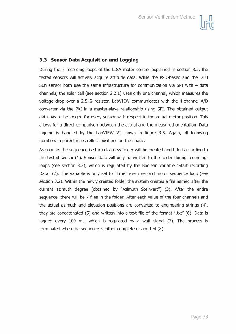
Sensor Verification Method
Page 38
3.3 Sensor Data Acquisition and Logging
During the 7 recording loops of the LISA motor control explained in section 3.2, the
tested sensors will actively acquire attitude data. While the PSD-based and the DTU
Sun sensor both use the same infrastructure for communication via SPI with 4 data
channels, the solar cell (see section 2.2.1) uses only one channel, which measures the
voltage drop over a 2.5 Ω resistor. LabVIEW communicates with the 4-channel A/D
converter via the PXI in a master-slave relationship using SPI. The obtained output
data has to be logged for every sensor with respect to the actual motor position. This
allows for a direct comparison between the actual and the measured orientation. Data
logging is handled by the LabVIEW VI shown in figure 3-5. Again, all following
numbers in parentheses reflect positions on the image.
As soon as the sequence is started, a new folder will be created and titled according to
the tested sensor (1). Sensor data will only be written to the folder during recording-
loops (see section 3.2), which is regulated by the Boolean variable “Start recording
Data” (2). The variable is only set to “True” every second motor sequence loop (see
section 3.2). Within the newly created folder the system creates a file named after the
current azimuth degree (obtained by “Azimuth Stellwert”) (3). After the entire
sequence, there will be 7 files in the folder. After each value of the four channels and
the actual azimuth and elevation positions are converted to engineering strings (4),
they are concatenated (5) and written into a text file of the format “.txt” (6). Data is
logged every 100 ms, which is regulated by a wait signal (7). The process is
terminated when the sequence is either complete or aborted (8).

Sensor Verification Method
Page 39
Figure 3–5: LabVIEW data logging VI

Sensor Verification Method
Page 40
3.4 Experiment Control
The overall schematics of the data processing setup discussed above can be taken
from figure 3-6. Data flow is always in both directions.
Figure 3–6: Schematics of the data processing setup
For observation and manual control of the testing process, an experiment control VI
was created. The gauges show the value of the global variables “Azimuth Position” and
“Elevation Position” (see section 3.2) at any time during a sequence. The front panel
also includes the manually operated functions of sequence start and abort, as well as
the command for the motor to return to its start position after a sequence has ended
or was aborted. For each sequence the sensor, which is being tested, is selected from
a drop down menu to give information on different procedures for data processing (see
section 3.3). Figure 3-7 shows this front panel. The block diagram to this VI can be
taken from the appendix section A3.

Sensor Verification Method
Page 41
Figure 3–7: LabVIEW experiment control front panel
3.5 The Test Setup
3.5.1 Simulation of the Space Environment
For validation of the accuracy of a Sun sensor, it is necessary to test it in a similar
environment as it will encounter in space. Obviously, there is no testing facility on
Earth with the exact same environment as in space, but there are ways to simulate
certain characteristics that have an impact on the functionality of the tested system.
One of these characteristics is the darkness in space. In Earth orbit there is, idealized,
only one light source: the Sun. To create this condition for the tested sensor, it has to
be exposed to only one light source, which simulates the Sun. All other possible light
sources (including reflections) have to be blocked.
This was realized using cartons as shields around the motor setup, leaving only one
opening for a light source. To reduce light reflections off the cartons they were spray-
painted matt black. This setup with the LISA motor is depicted in figure 3-8.

Sensor Verification Method
Page 42
Figure 3–8: Light shielding setup for the sensor test
3.5.2 Simulation of the Sun
For the simulation of the Sun it was necessary to find a directed light source, with
specifications similar to the Sun’s. The total solar irradiance, which arrives at the mean
Sun-Earth distance, is around [28]. In Earth-orbit the Sun has a color
temperature of around 6000 K [29]. Finding a light source that fulfills these criteria as
well as possible was crucial for the test setup. Most real Sun simulators are very costly,
which was the main reason for the choice of a conventional light. The following is a
description of the selected light source for this project. It best fulfilled the criteria out
of all considered and available lights.
The light source was rented at “TONEART mediavision” Augsburg, a supplier for
camera equipment. It uses a 1.2 kW metal-halide lamp (HMI1200) and is called
“Kobold DLf 1200S.” It is supplied with a voltage of 220 V at 50 Hz, AC (internally
converted to DC) and a current of 7 A. Its color temperature is specified to be about
6500 K, while its degree of efficiency is .

Sensor Verification Method
Page 43
The lamp itself and the final setup with the lamp and the LISA motor is shown in figure
3-9, where it is placed 1.55 (±0.05) m away from the tested sensor mounted on the
motor.
Figure 3–9: Kobold DLf 1200S metal-halide light for the sensor test setup
3.6 Sensor Data Evaluation
For sensor data evaluation, two different software programs were used: Microsoft
Excel and MathWorks MATLAB. Both versions are developed similarly to serve the
same purpose of plotting evaluation graphs.
3.6.1 Evaluation of the PSD-based Sun Sensor’s Data
The PSD-based sensor outputs data in four channels. Since LabVIEW writes raw data
with values of Z ϵ [0;1023] into the text files, they have to be converted to attain the
sensor’s measured azimuth and elevation degree. The values of Z represent the
comparison between the voltage output of transimpedance amplifier with AD8554 and
the reference voltage AD1582 (2.5 V). Z is 1023 when the sensor is not illuminated,
and 0 when the illumination evokes full-scale deflection. The values are distributed
over the 2.5 V of reference in single steps, which entails an increase of Z when the
voltage decreases:
(3-1)

Sensor Verification Method
Page 44
The constant q is therefore a single measured voltage step. This allows for calculation
of the output voltage ( ) of the transimpedance amplifier for each channel:
(3-2)
Knowing , the actual current at each anode of the PSD, amplified over a
resistor of 680 kΩ (R), can be calculated using Ohm’s law:
(3-3)
where is the reference voltage (2.5 V). When is obtained for all four PSD
anodes, the measured spot light position on the active area can be taken from formula
(2-4) and (2-5).
The following steps explain the acquisition of the azimuth and elevation degree based
on the sensor’s measurements.
At first the light spot position on the PSD has to be calculated for the position of origin
N (light beam perpendicular to the PSD’s surface) using the above mentioned formulas.
Next, the distance between point N and the calculated light spot position P (depending
on the current motor orientation) is attained with:
. (3-4)
Finally, the arctangent of
(3-5)
gives the absolute value of the calculated elevation degree. Constant h is the distance
between the PSD’s active area and the aperture plate, which is depicted in figure 3-10.
To differentiate angles in different directions and to obtain the real elevation angle
from the absolute values, an if-condition was implemented, which analyses whether
the measured x-position on the active area was smaller or larger than the value of the
x-coordinate of point N. If the value was smaller, the calculated elevation angle is
multiplied by -1 to yield a negative angle.

Sensor Verification Method
Page 45
Figure 3–10: PSD-based Sun sensor principle with calculation variables
The azimuth degree is the same as the angle between (for ) in azimuth
position 0°, and (for ) in the demanded azimuth degree. and are
specific coordinates of P for the respective azimuth degree. In the following the
variable a is the distance between and calculated analogical to formula (3-4).
Using the law of cosine, the arccosine of
(3-6)
equals the azimuth degree based on sensor measurements. Figure 3-11 shows these
points for exemplary values in the PSD’s active area coordinate system. The
implementation of these procedures in MATLAB (with comments) can be seen in the
appendix section A4.

Sensor Verification Method
Page 46
Figure 3–11: The azimuth degree on the PSD's active area (created using GeoGebra)
3.6.2 Evaluation of the DTU Sun Sensor’s Data
Just like the PSD-based sensor, the output data of the DTU sensor is divided into four
channels using the same range of assigned values. Every channel equals the converted
current evoked by one of the four diodes (see section 1.3). The conversion to voltage
is carried out by a transimpedance amplifier (see section 2.3.2.1). As explained in
section 1.3, the output values for Top and Bottom, and Left and Right respectively, are
normalized using the two equations (1-1). Because both normalized values are within a
defined range of ]-1;1[, they have to be multiplied by 90. The reason for this is that
the value of 0 is defined as full sensor illumination, which is reached when the motor is
in elevation position 0°, while values of almost 1 signal no sensor illumination. The
multiplied values are then plotted together with the actual motor orientation position,
which are also obtained via LabVIEW (see section 3.2). This is done using Excel.
3.6.3 Evaluation of Solar Cell 3G30C Data
Unlike the two sensors above, the payload solar cell outputs data only in one channel,
which has values of [0;32767] corresponding to voltages of 0 V and 10 V, respectively.
The values are proportional to the voltage drop over a 2.5 Ω resistor. The voltage drop
a

Sensor Verification Method
Page 47
is proportional to the current produced by the solar cell (max. 600 mA), which in turn
is dependent on the light’s incidence angle (see section 2.2.1). Formula (2-2), which
allows for calculation of the incidence angle θ knowing the radiant flux, is converted to
the following formula that expresses the angle’s connection to the cell’s output current:
(3-7)
of which is the measured current at θ, and is the current measured when the light
is in the cell’s zenith position. The currents are obtained via Ohm’s law with a resistor
value of 2.5 Ω. The arccosine of (3-9) yields the measured incidence angle. Since the
calculated angles have different dimensions than the actual motor position, they are
multiplied by 47.4 to fit the graph. This process is implemented in MS Excel.
3.6.4 Calculation of Sensor Measurement Error
To compare the sensors’ performance in elevation angle determination with each
other, the average measurement error (E) of the sensors’ calculated data and the
actual motor angle is computed. It is defined as the average distance (absolute values)
of all data points from the real elevation angle within a certain FOV or range [30]:
(3-8)
The formula, where n is the total quantity of sensor position measurements, is the
measured (calculated) elevation angle, and is the actual motor elevation angle,
directly reflects every tested sensor’s accuracy in elevation angle determination.

Test Results
Page 48
4 Test Results
4.1 Test Phase One
The test setup for the first sensor test can be seen in section 3.5. In the following, the
test results of each sensor are briefly summarized.
4.1.1 PSD-based Sun Sensor Test Results
For the first test of the PSD-based Sun sensor, spacers of 5 mm were used, which
leaves a distance of 3.74 mm between the aperture plate and the active area (see
section 2.3.3). The plot of the sensor’s raw output data for azimuth 0° (shown in figure
4-1) shows two large bulges (1), which signal heavy illumination, with minima at motor
elevation degrees around -30° and +30°. These unexpected bulges led to an incorrect
calculation of the elevation degree (see figure 4-2). Figure 4-2 is a plot of the values of
the actual motor elevation position and the elevation position calculated by the PSD,
which would be identical if the sensor delivered perfect data. The calculation process is
explained in section 3.6.1. The plot of figures 4-1 and 4-2 are very similar for all motor
azimuth degrees (sequence parts). The test eventually did not deliver valuable results.
Figure 4–1: Plot of PSD Sun sensor raw data for motor sequence part 1
(azimuth 0°)
0
200
400
600
800
1000
1200
90
84
,6
77
,9
71
,0
64
,8
57
,9
51
,2
45
,1
38
,2
31
,3
25
,4
19
,4
12
,4
5,7
-1,1
-8,0
-14
,2
-21
,3
-27
,3
-34
,0
-40
,6
-47
,4
-54
,0
-60
,6
-67
,5
-73
,6
-80
,1
-86
,5
Motor elevation degree
Anode Y1
Anode X1
Anode Y2
Anode X2
(1) (1)

Test Results
Page 49
Figure 4–2: Elevation degree based on PSD measurements for motor sequence part 1 (azimuth 0°)
4.1.2 DTU Sun Sensor Test Results
Figure 4-3 shows the DTU sensor’s raw data output of the four diodes (see section
3.6.2), again for motor azimuth sequence part of 0°. The normalized values multiplied
by 90 of diodes T and B, and L and R respectively (see section 1.3), are plotted in
figure 4-4. The fraction represents the measured elevation degree (for motor
azimuth 0°), while the fraction represents the steady azimuth angle (roughly 6°
due to the sensor’s mounting tilt) (see figure 1-12). Within the sensor’s specified FOV
of 140°, it has a measurement error of 8.5° from the actual elevation motor position.
As seen in the graph, the smaller the FOV is specified the smaller the measurement
error becomes. For the motor elevation range of 50° to -40° (see section 4.2) the
measurement error is 6.9°.
-100
-80
-60
-40
-20
0
20
40
60
80
100de
gree
s Motor elevation
elevation degree (ε)
measured by PSD

Test Results
Page 50
Figure 4–3: Plot of DTU Sun sensor raw data for motor sequence part 1 (azimuth 0°)
Figure 4–4: Elevation degree based on DTU Sun sensor measurements for motor sequence part 1 (azimuth 0°)
4.1.3 Solar Cell 3G30C Test Results
Just like in the other two tests, the solar cell delivered almost the same data for every
azimuth angle. Figure 4-5 shows the plot of the one-channel raw data for azimuth
0
100
200
300
400
500
600
700
800
900
90
84
,0
76
,5
70
,1
62
,8
55
,7
48
,2
41
,3
34
,0
27
,4
20
,0
13
,0
6,2
-0,3
-7,5
-15
,2
-22
,1
-29
,2
-36
,2
-43
,6
-50
,5
-58
,4
-64
,9
-72
,5
-79
,1
-85
,7
-83
,3
-90
Motor elevation degree
Left
Right
Bottom
Top
-100
-80
-60
-40
-20
0
20
40
60
80
100
degr
ees
Motor elevation
(90T)/B
(90L)/R

Test Results
Page 51
position 0°. Because of high noise level of the output data due to measurements
inaccuracies, a polynomial (power of 6) trendline (g(x)) was added to the graph.
Figure 4–5: Plot of solar cell 3G30C raw data for motor sequence part 1 (azimuth 0°)
As a result of the noisy output, the calculated incidence angle of formula (3-7), which
is depicted in figure 4-6, is based on the values of the trendline. The values are
absolute because the cell cannot differentiate between a positive and a negative
incidence angle (one angle output). For better comparison of the two graphs, the
motor elevation is also plotted for absolute values only. Within a FOV of 140° the
measurement error (with respect to the absolute motor elevation) is 2.1°. For the
range between +50° and -40° (90° FOV) the measurement error is 2.3°.
g(x) = 6E-12x6 - 9E-09x5 + 6E-06x4 - 0,0024x3 + 0,3434x2 - 6,4199x + 99,405
-500
0
500
1000
1500
2000
2500
30009
0
84
,1
78
,2
72
,1
64
,9
58
,1
51
,9
45
,3
38
,8
32
,8
26
,4
20
,1
13
,8
7,0
0,5
-6,4
-12
,9
-19
,3
-25
,7
-32
,6
-39
,3
-45
,9
-51
,9
-58
,3
-65
,0
-71
,5
-77
,6
-84
,3
Motor elevation degree
Cell's output
Poly. (Cell's output)

Test Results
Page 52
Figure 4–6: Elevation degree based on trendline of solar cell 3G30C measurements for motor sequence part 1 (azimuth 0°)
4.2 Test Phase Two
During testing phase two, the main focus was to enhance the PSD-based sensor’s
results. All other sensor results stayed the same as in test phase one. The sensor
problems of the first test were found after a detailed analysis of all test setup
components. The reason for the erroneous results was the sensor’s light shield, which
did not fulfill its purpose of protecting the sensor from unintentional exposure to light.
It was the motor’s sensor metal mounting platform that caused backlighting of the
circuit board through light reflection. This entailed full sensor illumination at motor
elevations of around -30° and +30° (see section 4.1.1). The circled area in figure 4-7
shows the reflecting surface. This problem was solved using duct tape, which was
taped all around the sensor to prevent the disruptive reflections (see figure 4-7).
0
10
20
30
40
50
60
70
80
90
100de
gree
s
absolute motor elevation
Measured Elevation
degree

Test Results
Page 53
Figure 4–7: Solution of sensor backlighting problems due to reflection
This new setup (using the same spacers) yielded entirely new data. The raw data can
be seen in figure 4-8, while the calculated elevation and azimuth degrees are shown in
figure 4-9. Both graphs represent motor sequence part 1, as in section 4.1. The results
are again similar for all azimuth positions. The measurement error between motor
elevation position +50° and -40° and the calculated elevation position in that range is
1.08°. In the same confinement the calculated azimuth angle has values of roughly
0.6° (excluding the midrange 180° maximum) that reflect the measured mounting tilt.

Test Results
Page 54
Figure 4–8: Plot of PSD-based Sun sensor raw data for motor sequence part 1 (azimuth 0°)
Figure 4–9: Elevation degree based on PSD Sun sensor measurements for motor sequence part 1 (azimuth 0°)
0
200
400
600
800
1000
1200
90
84
,6
78
,1
70
,9
64
,1
57
,6
51
,3
44
,3
37
,3
31
,3
24
,8
18
,5
11
,6
5,4
-1,5
-8,0
-14
,8
-21
,9
-28
,8
-35
,3
-42
,5
-47
,9
-55
,4
-62
,5
-68
,6
-75
,4
-82
,2
-89
,1
Motor elevation degree
Anode Y1
Anode X1
Anode Y2
Anode X2
-150
-100
-50
0
50
100
150
200
degr
ees
Motor elevation
elevation degree (ε)
measured by PSD
azimuth degree (α)
measured by PSD

Performance Evaluation and Discussion
Page 55
5 Performance Evaluation and Discussion
5.1 Motor Sequence Error
The reason for the identical results of sensor azimuth degree calculation for all motor
azimuth positions is a minor flaw in the experiment setup. Each sequence part (see
section 3.2) is programmed to run the elevation degree from -90° to +90° for all 7
azimuth positions from 0° to 90°. Since the light source is fixed, and the elevation
motor turns around the new azimuth axis (solid line in figure 5-1) for every sequence
part, the sensors are not able to recognize a change in azimuth degree. To avoid this
problem, the motor has to be programmed to turn around its azimuth 0° axis (dashed
line in figure 5-1) for every sensor azimuth position. While this determination problem
is solved for satellites by using several sensors, which are mounted orthogonally, a
single sensor can only determine two out of the pitch, roll and yaw angles.
Figure 5–1: The LISA motor's faulty azimuth turning axis (solid line)
This flaw has only little impact on the Solar Cell 3G30C test results, because the cell
can only determine the incidence angle in one dimension anyhow and therefore does
not recognize a second angle change. Again, more angle determinations can be

Performance Evaluation and Discussion
Page 56
achieved by the use of more cells, mounted in different positions. As a result, the cell’s
output data would not visibly change even if the motor sequence flaw was corrected.
The DTU sensor on the other hand, is, just like the PSD-based sensor, capable of
determining two angle rotations. While both sensors precisely reflect the motor’s
elevation degree, the azimuth degree seems to stay the same during all 7 sequence
parts. This means that, with this setup, the two sensors can only be directly compared
in one angle determination – the elevation angle.
For the PSD-based sensor, predictions can be made on what it is expected to output
for different azimuth degrees. Figures 5-2 and 5-3 show the calculated light spot
positions on the PSD’s active area within its FOV throughout two different motor
sequence parts (0° and 45°). The light spot positions together form a straight line,
which is tilted by as much as the sensor was tilted on its mount (due to mounting
inaccuracies). On the active area the two axes are interchanged, so the y-axis runs
horizontally. Because of the above stated sequence problem, both plots appear to be
exactly the same. The plot that would be expected, if the problem was corrected is
depicted by the dashed line (figure 5-3), which is rotated around point N (see section
3.6.1) by α (azimuth; in this case 45°) degrees. This prediction is based on the in
section 3.6.1 introduced azimuth degree calculation. The azimuth graph of figure 4-9
has a constant value of about 0.6° (excluding the 180° maximum), which equals the
sensor’s measured mounting tilt. All in all, the motor sequence problem is only a minor
drawback for the testing of the PSD-based sensor, because the Sun vector generation
(section 2.2.2) accuracy is only directly affected by light spot and hole (in the aperture
plate) position accuracy, which can be specified using the available test results that
directly depend on the same two parameters.
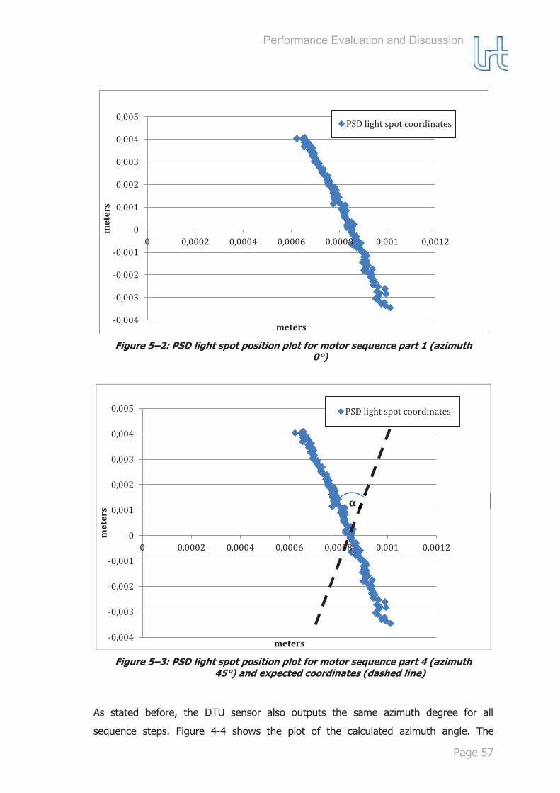
Performance Evaluation and Discussion
Page 57
Figure 5–2: PSD light spot position plot for motor sequence part 1 (azimuth
0°)
Figure 5–3: PSD light spot position plot for motor sequence part 4 (azimuth
45°) and expected coordinates (dashed line)
As stated before, the DTU sensor also outputs the same azimuth degree for all
sequence steps. Figure 4-4 shows the plot of the calculated azimuth angle. The
-0,004
-0,003
-0,002
-0,001
0
0,001
0,002
0,003
0,004
0,005
0 0,0002 0,0004 0,0006 0,0008 0,001 0,0012
met
ers
meters
PSD light spot coordinates
-0,004
-0,003
-0,002
-0,001
0
0,001
0,002
0,003
0,004
0,005
0 0,0002 0,0004 0,0006 0,0008 0,001 0,0012
met
ers
meters
PSD light spot coordinates
α

Performance Evaluation and Discussion
Page 58
average azimuth value is around 6°, which equals the slight tilt of the sensor mount
(the values show that this sensor was tilted more than the PSD-based sensor). Despite
the motor sequence drawback, the sensors can be compared in their elevation degree
determination accuracy over 7 different alignment positions.
5.2 Performance Comparison of All Three Tested Sensors
The test results of section 4 render each sensor’s measurement error in calculating the
motor elevation degree for several azimuth positions. Since vector calculation is based
on these angle measurements, the specified measurement error directly represents
Sun vector generation accuracy. The more accurate a sensor determines the Sun
vector, the better its attitude determination. For elevation degree determination the
PSD-based Sun sensor performed best in accuracy with a measurement error of only
1.08° within a FOV of 90°, while it featured a more limited FOV (with the use of 5 mm
spacers) than the other two tested systems, which is seen in figure 4-9. In this same
FOV (90°) the DTU sensor achieved a measurement error 6.9°. Both its average
experiment errors within the 90° and 140° FOV (8.5° error) are well above the
specified accuracy of 1° within the 140° FOV. The reason for that is that the specified
accuracy is the result of tests performed by Pedersen and Hales [18] at DTU with a
different interface and circuit board. The interface and circuit board designed by
Thomas Bickel (see section 1.3) therefore causes unforeseen inaccuracies for the
sensor. This assumption is indicated by the noise of the sensor’s output raw data seen
in figure 4-3. Noise is also a vital problem for the tested solar cell. It did not deliver
stable and reliable data that could have been used for attitude determination. Hence,
the values of the trendline were used to calculate the incidence angle, which leaves the
calculated accuracies for a FOV of 90° and 140° as estimates. This problem could be
solved by attentively investigating the cell’s circuit for error sources. Furthermore, the
cell only allows for calculation of one orientation angle. Since there are only four cells
mounted on different sides of the CubeSat, the overall constellation does not facilitate
unambiguous attitude determination for the satellite. Another drawback regarding solar
cell attitude determination is the fact that the cells are the satellite’s experimental
payload and have to be evaluated, where it is more reasonable to determine
indispensable evaluation information for the cells externally.

Performance Evaluation and Discussion
Page 59
The requirement of 1° accuracy (see section 2.1) is not entirely met by any of the
tested systems. The PSD-based sensor is nevertheless very close with its 1.08°
measurement error and therefore qualifies best as a suitable concept for attitude
determination on MOVE.
Referring to section 2.1, the PSD-based sensor at this level fulfills nearly all
requirements. The only parameters that still have to be evaluated for the smaller PSD
version (S5990-01) are the expansion of the FOV to 140° (using smaller spacers), 1°
accuracy, the sensor weight of 120 mg, and the thermal constraints (with the possible
use of heaters).
5.3 Attitude Determination for MOVE Using the PSD-based Sun Sensor
5.3.1 Error Accumulation
It is impossible for any sensor to determine attitude with 100% accuracy. There are
always error sources that have to be found and defined. The sum of all error sources is
directly proportional to the measurement error of the sensor, which can be lowered as
error sources are eliminated.
For the PSD-based sensor, error sources include PCB component inaccuracies, limited
light spot resolution on the active area, as well as mounting and hardware construction
inaccuracies. The voltage reference AD1582, mounted on the PCB, has a specified
output tolerance of ±0.2 V [25], which increases the noisiness of the measurement. As
observed in LabVIEW, the dimension-less output data of each channel has an
inaccuracy of ±3. This includes the error sources created by the other components on
the PCB. In addition, the PSD itself has a specified position detection error of ±150 μm
[21]. Furthermore, the construction of the entire sensor unveils new possible error
sources, of which the extent can hardly be measured. They include the distance
between the active area and the aperture plate (h) and the hole size. Minor deflections
of both dimensions have to be taken into account. Simultaneously, the hole size
directly affects the intensity of light diffraction (although its scale is very small). An
error parameter that cannot be eliminated, unless the hole size is variable, is the
recommendation [21] of a spot light size larger than ø 0.2 mm 80% from the center of
the active area to the edge, which entails minor inaccuracies, if not accounted for.
All these parameters in total are responsible for the sensor’s measurement error of
1.08°.

Performance Evaluation and Discussion
Page 60
5.3.2 The PSD-based Sensor’s Functionality in Space
As already mentioned, a test setup never resembles the exact same environment as
the sensor will encounter in space. For the PSD-based sensor a few test parameters
change when the sensor is actually in orbit. One of those parameters is the sensor’s
zero degree position. While point N has coordinates N(x≠0 ; y≠0) due to mounting
inaccuracies in the test setup, which limit light source alignment with the coordinate
system’s origin of the sensor, the aperture plate can be aligned with the active area to
nearly output a value of 0 for both coordinates when the Sun is in the sensor’s zenith
position in space. (Note: limited construction accuracy will always cause a minor shift
of point N from the PSD coordinate system’s origin) With point N being nearly N(x=0 ;
y=0) the sensor will have an evenly distributed FOV to all sides. Simultaneously this
explains why the elevation degree measured by the PSD (figure 4-9) loses accuracy
sooner when rotating in the negative elevation direction than when rotating in the
other. There is simply less active area space on one side of point N than on the other.
In the test setup this phenomenon entails a FOV of -40° to +50°. With proper
alignment, a FOV of almost -45° to +45° (with the same spacers) could be reached in
space.
As an alternative to the calculations of section 3.6.1, the satellites rotational angles can
also be calculated using the known Sun vector. The vector obtained with formula (2-3)
uses only light spot coordinates and the distance between the active area and the PSD
(h), which define the real Sun vector in its own coordinate system. For the sensor in
space, the two rotational angles that correlate with azimuth and elevation can be
obtained from the Sun vector and the coordinate system’s axes (see figure 5-4).
Another aspect that has to be kept in mind when finally integrating the sensor is the
mathematical singularity of angle calculations. The consequence of this issue can be
seen in figure 4-9, where the calculated azimuth degree at motor elevation positions
around 0° has a value of 180° because the position is mathematically not clearly
defined.

Performance Evaluation and Discussion
Page 61
Figure 5–4: Correlating azimuth and elevation angles against the Sun vector
To finally be able to determine attitude for the satellite in all positions, several single
sensors have to be mounted on different sides of the cube structure to cover the entire
sphere around the spacecraft. MOVE currently hosts four Sun sensor mounts of 14 x
22 mm (designed for the DTU sensor). Only the sensors, which have the Sun in their
current FOV will output the vector. This is handled via a filter system of the OBDH (on-
board data handling) board. This filter system ideally extracts only usable data, which
are obtained by the sensor within its specified FOV. Data that is usable but demands
modification, like the above mentioned singularity issue, is also filtered and substituted
for by this system. Exemplary, a look up table would assign the value of 0° for a
calculated azimuth degree of 180°.
5.4 Sensor Integration Considerations for MOVE
As already mentioned, MOVE has four sensor mounts installed. They are all on the
cube sides with the experimental payload so that whenever the payload is tested
attitude information is available. Figure 5-5 shows the flight PCB layout of the top and
bottom side as designed for the DTU sensor by Thomas Bickel [16].

Performance Evaluation and Discussion
Page 62
Figure 5–5: Top (right) and bottom (left) side of MOVE's Sun sensor flight PCB [16]
The bottom side shows the same PCB components as they are used on the PSD Sun
sensor’s test PCB (see figure 2-7). Therefore when integrating the small version of the
PSD (S5990-01) on the top side only minor connection and layout changes have to be
made. Finally, a suitable aperture plate that protects the PSD from undesired exposure
to light has to be designed, while keeping in mind the total height constraint of 6 mm
(see section 2.1). It is especially important to avoid backlighting of the circuit board.
One of the mounted flight PCBs with the DTU sensors on MOVE are depicted in figure
5-6 (circled area).

Performance Evaluation and Discussion
Page 63
Figure 5–6: MOVE satellite with current PCB flight model for the DTU Sun sensor
The two extravehicular wings of the satellite limit the sensor’s FOV due to shading.
This aspect has to be kept in mind when determining attitude. A possible way to avoid
problems caused by the wings is to identify satellite orientation positions where this
phenomenon occurs and to discard the false attitude information when approaching
the position.
All in all, the PSD-based sensor’s concept fully supports the needs of the CubeSat and
therefore has the potential of being integrated as a follow-up flight model.
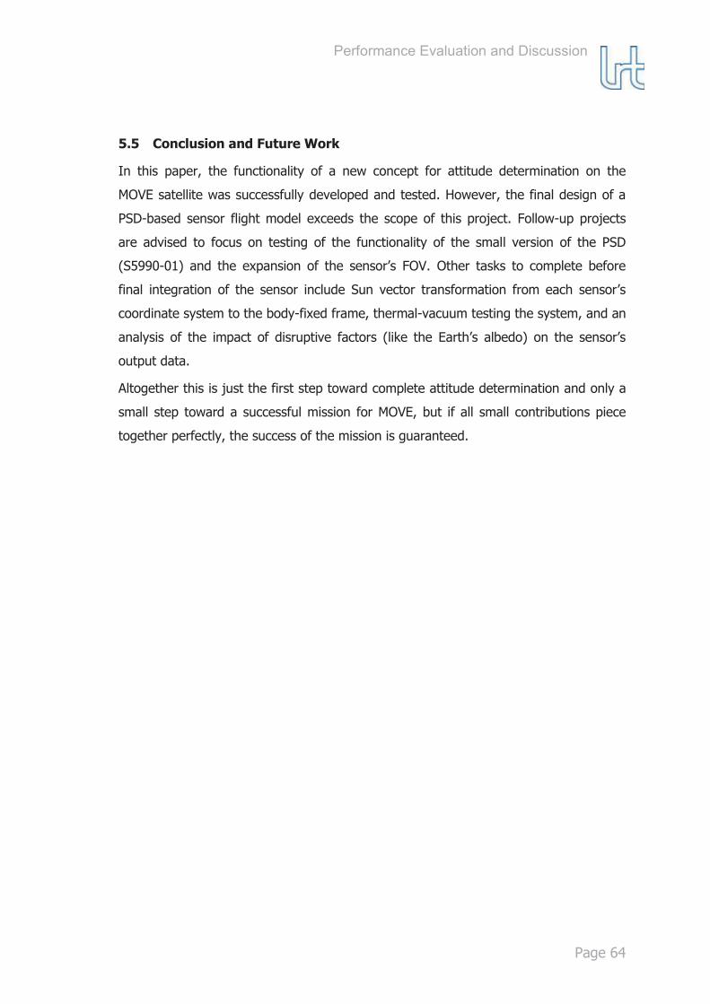
Performance Evaluation and Discussion
Page 64
5.5 Conclusion and Future Work
In this paper, the functionality of a new concept for attitude determination on the
MOVE satellite was successfully developed and tested. However, the final design of a
PSD-based sensor flight model exceeds the scope of this project. Follow-up projects
are advised to focus on testing of the functionality of the small version of the PSD
(S5990-01) and the expansion of the sensor’s FOV. Other tasks to complete before
final integration of the sensor include Sun vector transformation from each sensor’s
coordinate system to the body-fixed frame, thermal-vacuum testing the system, and an
analysis of the impact of disruptive factors (like the Earth’s albedo) on the sensor’s
output data.
Altogether this is just the first step toward complete attitude determination and only a
small step toward a successful mission for MOVE, but if all small contributions piece
together perfectly, the success of the mission is guaranteed.

Appendix References
Page 65
A Appendix
A.1 References [1] Claas Olthoff MOVE overview. A First-MOVE in satellite development at TUM
(TUM Institute of Astronautics). [2] Dr. Mitch Bryson 2011 Satellite Attitude Determination 1. AERO4701 Space
Engineering 3. lecture handouts for the Australian Centre for Field Robotics, University of Sydney. Available at http://www-personal.acfr.usyd.edu.au/m.bryson/Lectures/lecture_week7_handouts.pdf. Accessed: 12/01/11
[3] Wiley J. Larson and James R. Wertz ed 2006 Space Mission Analysis and Design. Third Edition (Microcosm Press, CA and Springer, NY).
[4] Wikipedia 2011 Datum (geodesy). Available at http://en.wikipedia.org/wiki/Datum_%28geodesy%29. Accessed: 12/01/11
[5] Dr. Mitch Bryson 2011 AERO4701: Space Engineering 3. lecture handouts for the Australian Centre for Field Robotics, University of Sydney. Available at http://www-personal.acfr.usyd.edu.au/m.bryson/Lectures/lecture_week1_handouts.pdf. Accessed: 12/01/11
[6] Wikipedia 2011 Nadir. Available at http://en.wikipedia.org/wiki/Nadir. Accessed: 12/02/11
[7] Michael D. Griffin and James R. French 2004 Space Vehicle Design (American Institute of Aeronautics and Astronautics, Inc.).
[8] NASA 2011 NASA's Gravity Probe B Confirms Two Einstein Space-Time Theories. NASA's Latest News. Available at http://www.nasa.gov/mission_pages/gpb/gpb_003.html. Accessed: 12/02/11
[9] Texas Instruments Accelerometeres and How they Work. Available at http://www2.usfirst.org/2005comp/Manuals/Acceler1.pdf. Accessed: 12/07/11
[10] Wikipedia 2011 Talk: South Pole. Available at http://en.wikipedia.org/wiki/Talk%3ASouth_Pole. Accessed: 12/04/11
[11] NASA 1970 Spacecraft Sun Sensors. Available at http://www.dept.aoe.vt.edu/~cdhall/courses/aoe4065/NASADesignSPs/sp8047.pdf. Accessed: 12/03/11
[12] NASA 1969 Spacecraft Earth Horizon Sensors. Available at http://ntrs.nasa.gov/archive/nasa/casi.ntrs.nasa.gov/19700026254_1970026254.pdf. Accessed: 12/01/11
[13] Ball Aerospace and Technologies Corp. Star Trackers. Available at http://www.ballaerospace.com/page.jsp?page=104. Accessed: 12/07/11
[14] Ming Wang Passive Magnetic Attitude Stabilization. [15] Nick Sweet 2011 Hysteresis in Plain English. Attitude Control System. Available at
http://spaceconcordia.ca/2011/10/hysteresis-in-plain-english/. Accessed: 12/14/11
[16] Thomas Bickel 2009 Electrical Design and Integration of Sun Sensors for the Picosatellite MOVE.
[17] AZUR SPACE 2009 30% Triple Junction GaAs Solar Cell. Type: TJ Solar Cell 3G30C.

Appendix References
Page 66
[18] Martin Pedersen and Jan Hales 2004 Linear Two-Axis MOEMS Sun Sensor. Part of the DTUsat project - and beyond. Available at http://hvig.dk/files/Pedersen-and-Hales-2004-Linear-Two-Axis-MOEMS-Sun-Sensor-Technical-Report.pdf. Accessed: 12/17/11
[19] ISIS - Innovative Solutions In Space Miniaturised Analog Fine Sun Sensor. Available at http://www.isispace.nl/brochures/ISIS_MINI_FSS_Brochures_v.7.11.pdf. Accessed: 12/17/11
[20] Holger Adomat 2010 Grundlagen einer PVAnlage / Sonnenenergie. Available at http://www.nibis.ni.schule.de/~ruzbbsof/PDF%20Formate/Infoblatt%202.pdf. Accessed: 12/18/11
[21] Hamamatsu Photonics K.K. S S D 2007 Two-dimensional PSD S5990-01, S5991-01. Improved tetra-lateral type for surface mounting.
[22] EU-Kooperationsbüro Bayern Innovativ GmbH 2011 Time-saving Printed Circuit Board Production Technology. Available at http://www.technologiepartner.de/index.php?file=bbs-show.php&bbsref=11%20TR%2099PB%203KQD&PHPSESSID=k16ciap6jjb5939eibluunup61. Accessed: 01/07/12
[23] Analog Devices Zero-Drift, Single-Supply, Rail-to-Rail Input/Output Operational Amplifiers. AD8551/AD8552/AD8554. Available at http://www.analog.com/static/imported-files/data_sheets/AD8551_8552_8554.pdf. Accessed: 12/23/11
[24] Wikipedia 2011 Transimpedanzverstärker. Available at http://de.wikipedia.org/wiki/Transimpedanzverst%C3%A4rker. Accessed: 01/05/12
[25] Analog Devices 2.5 V to 5.0 V Micropower, Precision Series Mode Voltage References. AD1582/AD1583/AD1584/AD1585. Available at http://www.analog.com/static/imported-files/data_sheets/AD1582_1583_1584_1585.pdf. Accessed: 12/23/11
[26] Microchip Technology Inc. 2008 MCP3004/3008. 2.7 V 4-Channel/8-Channel 10-Bit A/D Converters with SPI Serial Interface. Available at http://ww1.microchip.com/downloads/en/DeviceDoc/21295C.pdf. Accessed: 12/23/11
[27] Dr. David P. Stern 2004 Coordinates. Azimuth and Elevation. Available at http://www-istp.gsfc.nasa.gov/stargaze/Scelcoor.htm. Accessed: 12/23/11
[28] NASA 2011 Climate & Radiation. Solar Radiation. Available at http://atmospheres.gsfc.nasa.gov/climate/index.php?section=136. Accessed: 12/14/11
[29] Jordan Butler The Sun: Light and Color Temperature. Available at http://www.sewanee.edu/chem/Chem&Art/Detail_Pages/ColorProjects_2004/Butler/Butler.html. Accessed: 12/26/11
[30] Universität zu Köln Fehlerrechnung. Available at http://www.ph2.uni-koeln.de/fileadmin/Lehre/Anfaengerpraktikum/Fehler.pdf. Accessed: 01/04/12

Appendix PSD PCB Connection Diagram
Page 67
A.2 PSD PCB Connection Diagram
Appendix to section 2.3.2:
Figure A-1: TARGET connection diagram for the PSD test-PCB

Appendix LabVIEW Experiment Control VI
Page 68
A.3 LabVIEW Experiment Control VI Appendix to section 3.5:
Figure A-2: LabVIEW block diagram for the experiment control VI
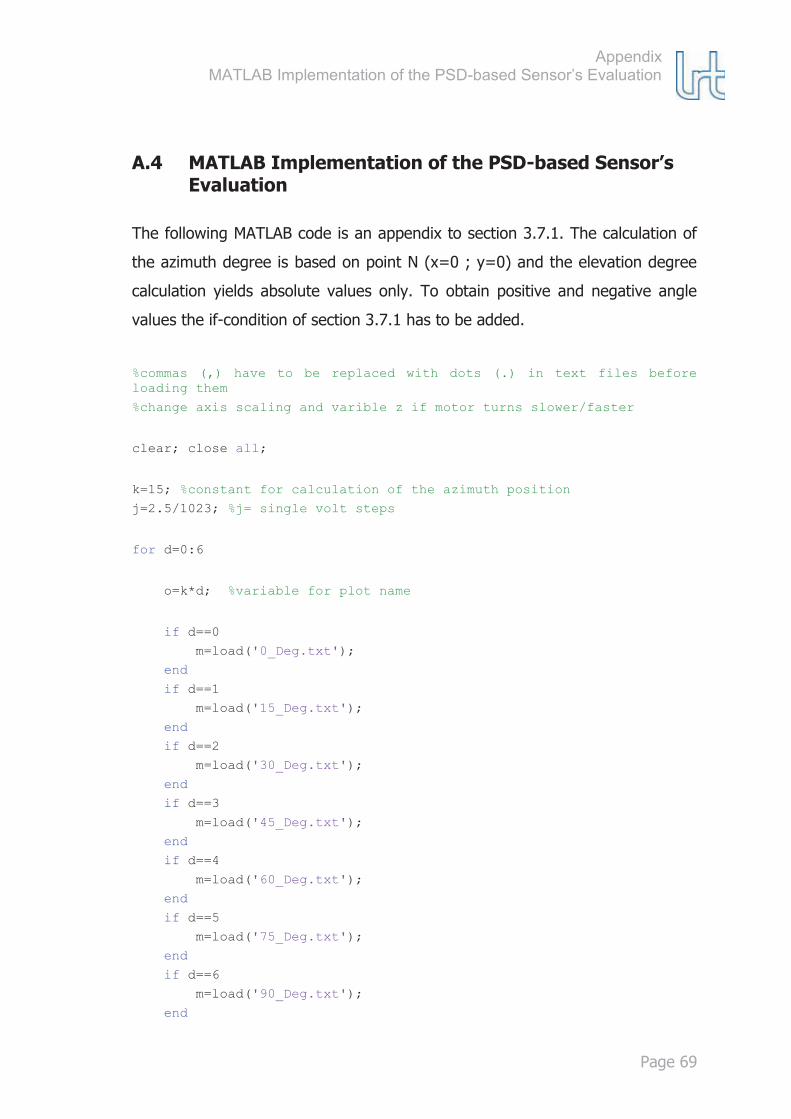
Appendix MATLAB Implementation of the PSD-based Sensor’s Evaluation
Page 69
A.4 MATLAB Implementation of the PSD-based Sensor’s Evaluation
The following MATLAB code is an appendix to section 3.7.1. The calculation of
the azimuth degree is based on point N (x=0 ; y=0) and the elevation degree
calculation yields absolute values only. To obtain positive and negative angle
values the if-condition of section 3.7.1 has to be added.
%commas (,) have to be replaced with dots (.) in text files before loading them %change axis scaling and varible z if motor turns slower/faster clear; close all; k=15; %constant for calculation of the azimuth position j=2.5/1023; %j= single volt steps for d=0:6 o=k*d; %variable for plot name if d==0 m=load('0_Deg.txt'); end if d==1 m=load('15_Deg.txt'); end if d==2 m=load('30_Deg.txt'); end if d==3 m=load('45_Deg.txt'); end if d==4 m=load('60_Deg.txt'); end if d==5 m=load('75_Deg.txt'); end if d==6 m=load('90_Deg.txt'); end

Appendix MATLAB Implementation of the PSD-based Sensor’s Evaluation
Page 70
for z=1:270 realElevation=m(z,3); %calculation of azimuth and elevation angle measured by the PSD kVoltAmplifier1 = m(z,4) * j; kVoltAmplifier1Var = 2.5 - kVoltAmplifier1; kCurrentAnodeY1 = kVoltAmplifier1Var / 680000; kVoltAmplifier2 = m(z,5) * j; kVoltAmplifier2Var = 2.5 - kVoltAmplifier2; kCurrentAnodeX1 = kVoltAmplifier2Var / 680000; kVoltAmplifier3 = m(z,6) * j; kVoltAmplifier3Var = 2.5 - kVoltAmplifier3; kCurrentAnodeY2 = kVoltAmplifier3Var / 680000; kVoltAmplifier4 = m(z,7) * j; kVoltAmplifier4Var = 2.5 - kVoltAmplifier4; kCurrentAnodeX2 = kVoltAmplifier4Var / 680000; kVar1 = kCurrentAnodeX2 + kCurrentAnodeY1; kVar2 = kCurrentAnodeX1 + kCurrentAnodeY2; kVar3 = kVar1 - kVar2; kVar4 = kCurrentAnodeX1 + kCurrentAnodeX2 + kCurrentAnodeY1 + kCurrentAnodeY2; kVar5 = kVar3 / kVar4; kVar6 = kVar5 * 0.01; %size of PSD active area: 0.01 by 0.01 meters kPosX = kVar6 / 2; kVarr1 = kCurrentAnodeX2 + kCurrentAnodeY2; kVarr2 = kCurrentAnodeX1 + kCurrentAnodeY1; kVarr3 = kVarr1 - kVarr2; kVarr5 = kVarr3 / kVar4; kVarr6 = kVarr5 * 0.01; kPosY = kVarr6 / 2; %conversion of x and y position of the light spot into measured (by %PSD)elevation and azimuth degree: PN=sqrt((kPosX-6.0241*10^-5)^2+(kPosY-6.0241*10^-5)^2); %distance between PSD light point and PSD reference (center) light point
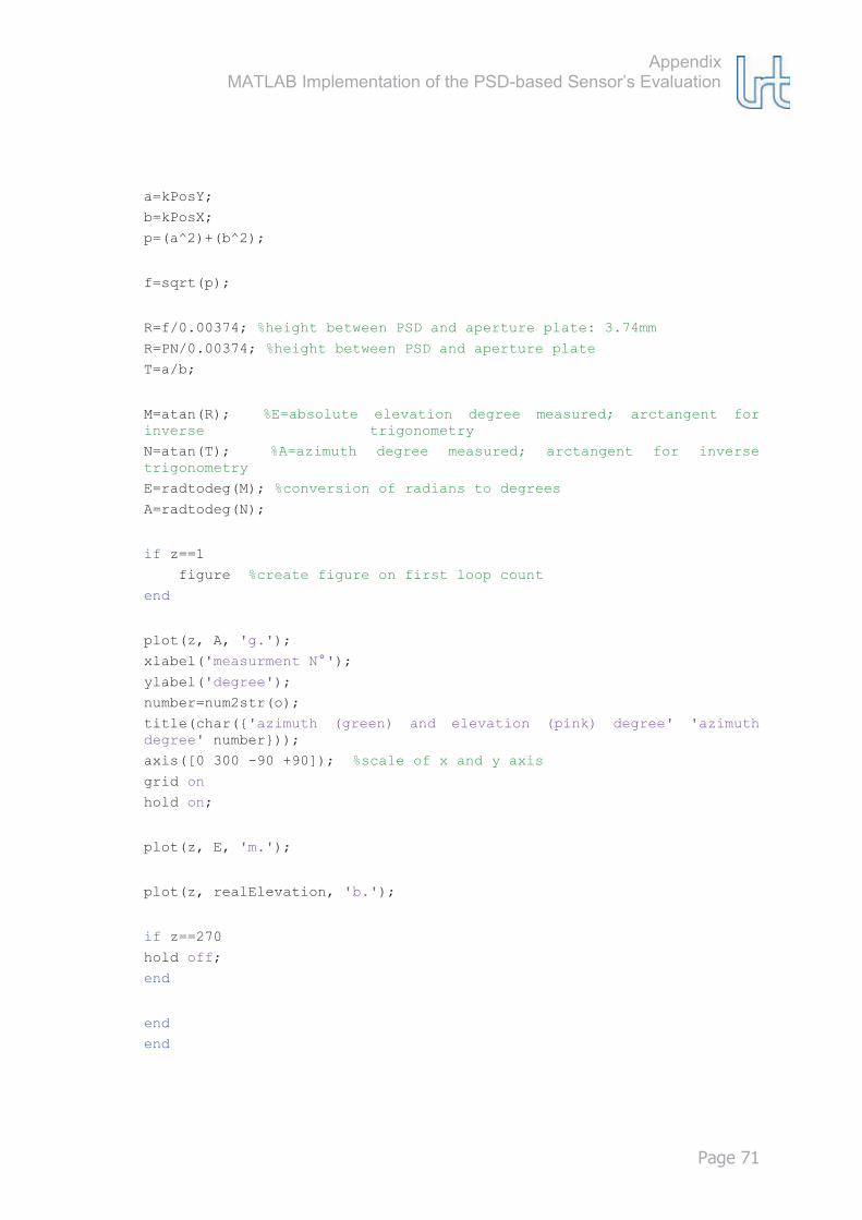
Appendix MATLAB Implementation of the PSD-based Sensor’s Evaluation
Page 71
a=kPosY; b=kPosX; p=(a^2)+(b^2); f=sqrt(p); R=f/0.00374; %height between PSD and aperture plate: 3.74mm R=PN/0.00374; %height between PSD and aperture plate T=a/b; M=atan(R); %E=absolute elevation degree measured; arctangent for inverse trigonometry N=atan(T); %A=azimuth degree measured; arctangent for inverse trigonometry E=radtodeg(M); %conversion of radians to degrees A=radtodeg(N); if z==1 figure %create figure on first loop count end plot(z, A, 'g.'); xlabel('measurment N°'); ylabel('degree'); number=num2str(o); title(char({'azimuth (green) and elevation (pink) degree' 'azimuth degree' number})); axis([0 300 -90 +90]); %scale of x and y axis
grid on hold on; plot(z, E, 'm.'); plot(z, realElevation, 'b.'); if z==270 hold off; end end end