development and implementation of a compensation …
TRANSCRIPT
DEVELOPMENT AND IMPLEMENTATION OF A COMPENSATION TECHNIQUE
FOR LUMINESCENCT SENSORS
A Dissertation
by
BRADLEY BRUCE COLLIER
Submitted to the Office of Graduate and Professional Studies of
Texas A&M University
in partial fulfillment of the requirements for the degree of
DOCTOR OF PHILOSOPHY
Chair of Committee, Michael J. McShane
Committee Members, Gerard L. Coté
Javier A. Jo
Sandun D. Fernando
Head of Department, Gerard L. Coté
December 2013
Major Subject: Biomedical Engineering
Copyright 2013 Bradley Bruce Collier
ii
ABSTRACT
Despite offering high specificity and speed compared to other methods, the
dependency of the response of an enzymatic sensor on ambient oxygen concentrations.
To investigate this issue, a reaction-diffusion model was developed using the finite
element method. Due to the growing population of people with diabetes, glucose was
chosen as a model analyte. This glucose sensor model was used to examine the oxygen
dependency and the resulting inaccuracy of glucose predictions. To improve the
accuracy of glucose predictions, an oxygen compensation method was developed which
utilizes a variable calibration curve where the fit parameters are dependent on the
ambient oxygen concentration. This allows a unique calibration curve to be obtained for
every oxygen concentration. Glucose predictions made with this compensation
technique were found to be within clinically acceptable regions more than 95% of the
time whereas predictions made without compensation were clinically acceptable less
than 50% of the time.
In order to apply this compensation technique for real-time analysis, ambient
oxygen concentrations must be measured in parallel with the response of the glucose
sensor. Despite the growing need for multi-analyte sensors such as this, a suitable
method for monitoring multiple responses in vivo has yet to be developed. Due to the
measurement flexibility provided by luminescence, a time-domain luminescence lifetime
measurement system was developed. The Dynamic Rapid Lifetime Determination
(DRLD) approach utilizes a dynamic windowing algorithm to select the optimal window
width for calculation of lifetimes using an integrative approach. This method was

iii
demonstrated with an oxygen-sensitive luminophore and shown to accurately determine
lifetime values six orders of magnitude faster than traditional methods.
This method was then extended to simultaneous measurement of the lifetimes
from two luminophores (Dual DRLD or DDRLD) for multi-analyte applications. The
ability of DDRLD to calculate lifetimes was demonstrated using temperature and oxygen
sensing films. Similar to oxygen compensation of glucose sensors, a temperature
compensation method was investigated for oxygen sensors. Lifetimes of the temperature
sensing films for dual films measurements made using DDRLD were not significantly
different than individual film measurements using DRLD. Oxygen responses for dual
films followed the same trend as individual film measurements and displayed a minimal
difference on average (2%). Real-time, dynamic temperature and oxygen predictions
were demonstrated using DDRLD in conjunction with temperature compensation of the
oxygen sensing film response.

iv
ACKNOWLEDGEMENTS
I would like to thank my committee chair, Dr. McShane, and my committee
members, Dr. Coté, Dr. Jo, and Dr. Fernando, for their guidance and support throughout
the course of this research.
Thanks also go to my friends, colleagues, and the department faculty and staff for
making my time at Texas A&M University a great experience. I also want to extend my
gratitude to the Texas A&M University Association of Former Students, which provided
me funding in the form of a Graduate Merit Fellowship.
Finally, thanks to my mother and father for their encouragement and to my wife
for her patience and love.
v
TABLE OF CONTENTS
Page
ABSTRACT .......................................................................................................................ii
ACKNOWLEDGEMENTS .............................................................................................. iv
TABLE OF CONTENTS ................................................................................................... v
LIST OF FIGURES ........................................................................................................ viii
LIST OF TABLES ......................................................................................................... xiii
1. INTRODUCTION .......................................................................................................... 1
2. GLUCOSE SENSOR BACKGROUND ........................................................................ 7
2.1 Measurements Utilizing Finger-Lancing ................................................................. 7 2.2 Commercial CGMS .................................................................................................. 8
2.2.1 Electrochemical ................................................................................................. 8 2.2.2 Microdialysis ................................................................................................... 10 2.2.3 Reverse Iontophoresis ..................................................................................... 10
2.3 Optical Methods of Glucose Detection .................................................................. 11 2.4 Luminescence ......................................................................................................... 12
2.4.1 Binding-Based Glucose Assays ....................................................................... 12 2.4.1.1 Concanavalin A ........................................................................................ 12
2.4.1.2 Glucose Binding Protein .......................................................................... 13 2.4.1.3 Apo-Enzymes ........................................................................................... 14
2.4.1.4 Boronic Acid ............................................................................................ 14 2.4.2 Enzymatic Sensors .......................................................................................... 14
2.4.2.1 Direct, Enzymatic Glucose Sensing ......................................................... 15 2.4.2.2 Indirect, Enzymatic Glucose Sensing ....................................................... 15
2.5 Oxygen-Dependence and Compensation of Enzymatic Glucose Sensors ............. 16
3. OXYGEN-DEPENDENCE AND COMPENSATION OF LUMINESCENT,
ENZYMATIC GLUCOSE SENSORS ........................................................................ 20
3.1 Theory of Enzymatic Sensor Model....................................................................... 21 3.2 Oxygen Response Measurements of a Hydrogel Sensor ....................................... 27
3.3 Results and Discussion ........................................................................................... 30 3.3.1 Modeled Glucose Sensor Response ................................................................ 30 3.3.2 Oxygen Dependent Response of Enzymatic, Glucose Sensors ....................... 35
3.4 Conclusions ............................................................................................................ 44

vi
4. BACKGROUND ON TIME-RESOLVED MEASUREMENTS OF
LUMINESCENCE ....................................................................................................... 45
4.1 Numerical Analysis ................................................................................................ 48 4.2 Phase-Plane Method ............................................................................................... 49
4.3 Maximum Likelihood Estimator ............................................................................ 51 4.4 Rapid Lifetime Determination ............................................................................... 51 4.5 Dual-Exponential Lifetime Decay Response Measurement Techniques ............... 53
5. DYNAMIC RAPID LIFETIME DETERMINATION ................................................ 58
5.1 Theory .................................................................................................................... 61
5.2 Experimental Details .............................................................................................. 63 5.2.1 Lifetime Techniques ........................................................................................ 63
5.2.2 Modeled Lifetime Responses .......................................................................... 64
5.2.3 Custom Lifetime Measurement System .......................................................... 65 5.3 In Vitro Testing and Comparison ........................................................................... 67
5.3.1 Oxygen Sensors and In Vitro Experimental Setup .......................................... 68
5.4 Results and Discussion ........................................................................................... 70 5.5 Conclusions ............................................................................................................ 75
6. DUAL DYNAMIC RAPID LIFETIME DETERMINATION .................................... 77
6.1 Theory .................................................................................................................... 80
6.2 Materials and Methods ........................................................................................... 84 6.2.1 Modeling of Dual Exponential Decays ........................................................... 85
6.2.2 Sensor Formulation ......................................................................................... 86 6.2.3 Instrumentation and Measurement .................................................................. 87 6.2.4 Film Testing and Analysis ............................................................................... 89
6.3 Results and Discussion ........................................................................................... 92 6.3.1 Results of Modeled Dual-Exponential Lifetime Calculations ........................ 92
6.3.2 Calibration of Individual Film Responses ....................................................... 92 6.3.3 Dual Film Responses ....................................................................................... 96
6.3.4 Dynamic Testing ............................................................................................. 98 6.4 Conclusions .......................................................................................................... 103
7. CONCLUSIONS AND FUTURE WORK ................................................................ 105
REFERENCES ............................................................................................................... 113
TIME-DOMAIN LIFETIME MEASUREMENT SYSTEM ............... 126 APPENDIX A.
A.1 Circuitry............................................................................................................... 127 A.1.1 Device Power ........................................................................................... 127
A.1.2 Excitation Circuit ..................................................................................... 129

vii
A.1.3 Detector Connections ............................................................................... 129 A.2 Optical Components ............................................................................................ 129
A.2.1 Excitation Signal ...................................................................................... 129 A.2.2 Emission and Collection ........................................................................... 130
A.3 Software............................................................................................................... 131 A.3.1 Excitation Signal Control ......................................................................... 133 A.3.2 Data Acquisition ....................................................................................... 133 A.3.3 Lifetime Calculation ................................................................................. 134 A.3.4 Data Storage ............................................................................................. 135
CUSTOM TESTING BENCH .............................................................. 136 APPENDIX B.
B.1 Glucose Concentration Control ........................................................................... 137
B.2 Oxygen Concentration Control ............................................................................ 138 B.3 Temperature Control............................................................................................ 140 B.4 Miscellaneous ...................................................................................................... 140
LIFETIME CALCULATION SOURCE CODE .................................. 141 APPENDIX C.
C.1 Dynamic Rapid Lifetime Determination Source Code........................................ 141 C.2 Dual Dynamic Rapid Lifetime Determination Source Code ............................... 143

viii
LIST OF FIGURES
Page
Figure 1.1 Generalized reaction scheme of glucose oxidase showing the substrates
consumed and products. ...................................................................................... 2
Figure 3.1 These graphs show reported reaction rate constants (blue circles) for
Equations 3.1 and 3.2 versus temperature. Predicted values at 37°C are
estimated (black diamonds) using linear regression (red lines) following a
logarithmic transformation. .............................................................................. 23
Figure 3.2 Oxygen distributions obtained for different glucose levels for a matrix
with and set to 1e-11m2/s, a bulk oxygen concentration of 80 μM,
and a GOx concentration of 1.8e-10 M. ........................................................... 25
Figure 3.3 The lifetime response of an oxygen-sensitive palladium porphyrin
immobilized in pHEMA. The inset shows the resulting Stern-Volmer
plot. Error bars represent standard deviation with n = 10................................ 29
Figure 3.4 Representative glucose responses for a range of oxygen and glucose
diffusion coefficients (represented in ratio form) as well as a range of
values. ............................................................................................................... 31
Figure 3.5 Modeled response of a sensor using different GOx concentrations and
with and set to 1e-11m2/s and a bulk oxygen concentration of 80
μM. .................................................................................................................... 32
Figure 3.6 Plots of the values obtained for parameters and versus transformed
GOx concentrations. Parameters were obtained by fitting the results in
Figure 3.5. The black line in each graph represents the optimal GOx
concentration for a range of 200 mg/dL. .......................................................... 33
Figure 3.7 This graph shows the oxygen dependent response for three different
model materials at four different oxygen concentrations. ................................ 34
Figure 3.8 This graph shows the modeled sensor response for = = 1e-11 m2/s,
[GOx]=1.62e-10 M, and a range of oxygen concentrations. The dashed
lines represent the fitting of the data for glucose values from 40 to 400
mg/dL. ............................................................................................................... 36

ix
Page
Figure 3.9 Fit parameters of Equation 3.8 as functions of oxygen concentration.
Blue circles show actual values obtained and dashed lines represent the fit. ... 37
Figure 3.10 This graph shows a Clarke error grid of predicted glucose versus actual
glucose concentrations for a range of oxygen concentrations. Circles
show values predicted using oxygen compensation and squares show
values predicted without oxygen compensation, assuming calibration was
performed at 80 μM. ......................................................................................... 38
Figure 3.11 This Clarke error grid shows glucose predictions obtained from
random oxygen and glucose values. Theoretical measurement error is not
included. Blue circles show oxygen compensated predictions and red
squares show uncompensated predictions. Markers that are filled in
represent negative or imaginary glucose predictions (see text). It should
be noted that these values only represent the presence of an erroneous
prediction and not an actual predicted glucose value. ...................................... 40
Figure 3.12 This graph shows the difference in actual and predicted glucose values
for the results in Figure 3.11 as a function of oxygen concentration. Blue
circles and red squares again represent, oxygen compensated and
uncompensated glucose predictions, respectively. Markers that are filled
in represent the presence of an erroneous measurement (see text). .................. 41
Figure 3.13 This Clarke error grid shows glucose predictions obtained from random
oxygen and glucose values. Theoretical measurement error was also
considered. Blue circles show oxygen compensated predictions and red
squares show uncompensated predictions. Markers that are filled in
represent negative or imaginary glucose predictions (see text). It should
be noted that these values only represent the presence of an erroneous
prediction and not an actual predicted glucose value. ...................................... 43
Figure 4.1 A) Diagram of an intensity-based ratiometric response where P1 is the
peak of an insensitive reference and P2 is the analyte sensitive
luminophore. B) Another intensity-based ratiometric response where both
P1 and P2 respond to the analyte of interest but in opposite directions. ............ 46
Figure 4.2 A) Multi-window technique utilized to determine lifetimes with the
PPM and MLE methods. B) Representation of a two-window approach
for RLD lifetime calculations. The variables , , and refer to the
start time, integrated intensity and initial intensity of the window. The
length of the window is represented by . ...................................................... 50

x
Page
Figure 4.3 Depiction of TD decays for two temporally-distinct dyes with lifetimes
of 5 and 1,000 μs. Inset is of the same decays but at a smaller period to
show the decay of the shorter-lived luminophore and the nearly constant
signal of the longer-lived luminophore. ............................................................ 54
Figure 4.4 Example of a contiguous, equi-width window implementation of dual
RLD lifetime calculations. ................................................................................ 55
Figure 4.5 This is a depiction of the pulsed excitation and emission of a dual
fluorescence and phosphorescence measurement. ............................................ 56
Figure 5.1 Diagram of the basic RLD lifetime determination approach with
contiguous windows of equal width. ................................................................ 60
Figure 5.2 Simplified low chart of dynamic windowing algorithm operation. ............... 62
Figure 5.3 Theoretical implementation over three different lifetimes of the four
static window methods utilized to compare to DRLD. is represented
by a light colored box and is represented by a dark colored box. Any
overlap of the windows is represented by a shade in between the two
window colors. .................................................................................................. 64
Figure 5.4 Examples of modeled luminescence decays with an SNR of 10. .................. 66
Figure 5.5 The lifetimes calculated for each window-sum based method in response
to a simulated profile can be found in the top portion of each graph while
the residuals of those calculations can be found on the bottom. The black
line represents the simulated lifetime for each point in time. ........................... 69
Figure 5.6 Example decays obtained from the custom lifetime measurement system
for each oxygen concentration tested. .............................................................. 71
Figure 5.7 Lifetime response profile of the different window-sum methods
compared to the lifetime calculated using traditional fittings. Error bars
represent 95% confidence interval with n=25. ................................................. 73
Figure 6.1 Diagram showing the combined response of a shorter-lived
luminophore, , and a longer-lived luminophore, . ..................................... 79

xi
Page
Figure 6.2 Depiction of a dual-exponential decay and the window sums utilized to
calculate the lifetime response using DDRLD. The black dashed line
represents the combined response, while the blue and red dashed lines
represent response of and , respectively. Example window sums are
shown in the shaded regions. ............................................................................ 81
Figure 6.3 Diagram showing a simplified version of the DDRLD algorithm. ................ 83
Figure 6.4 This picture shows examples of films tested. The sensor on the far left
is an oxygen sensing film containing PtOEP and the sensor on the right is
a temperature sensing film containing MFG. The sensor in the middle
consists of halves of each film placed side-by-side. ......................................... 87
Figure 6.5 Contour maps showing RSD values lifetimes calculated using DDRLD
for modeled decays with a range of and values. RSD for is in the left graph while RSD for is shown in the graph at the right. .......... 91
Figure 6.6 This graph shows the response of three individual MFG films (Runs 1-3)
and the averaged response. The red dotted line represents the linear fit of
the averaged response. Error bars represent the 95% confidence interval
with n = 10 for individual films and n = 3 for the averaged response. ............. 93
Figure 6.7 Response of individual PtOEP films to oxygen and temperature. Error
bars represent the 95% confidence interval with n = 10 for individual
films (Runs 1-3) and n = 3 for averaged data. .................................................. 94
Figure 6.8 Stern-Volmer response of the PtOEP films. The red line represents the
fit obtained using Equation 6.4 which was used for calibration. ...................... 95
Figure 6.9 Temperature ( ) dependent trends for , , and can be seen in
the top left, bottom left, and bottom right images, respectively. The red
lines show the linear fit obtained for each set of data. The top right image
shows the initial fractional intensities obtained where the red line
represents mean value that was used to obtain and . ........................ 96
Figure 6.10 Comparison of the MFG lifetime response for individual and dual film
experiments where lifetimes were calculated using DRLD and DDRLD,
respectively. Error bars represent the 95% confidence interval for n = 3
films. ................................................................................................................. 97

xii
Page
Figure 6.11 Comparison of lifetimes calculated for dual film experiments using
DDRLD and individual film experiments where lifetimes were calculated
using DRLD. Error bars represent 95% confidence intervals for n = 3
films. ................................................................................................................. 98
Figure 6.12 Results of a dynamic test showing programmed and predicted
temperatures. DDRLD was utilized to monitor the lifetime responses of
the two films simultaneously. Temperature predictions were determined
from a linear calibration curve. ......................................................................... 99
Figure 6.13 This graph depicts the programmed and predicted oxygen
concentrations from a dynamic test. DDRLD was utilized to monitor the
lifetime responses of the two films simultaneously. A temperature
compensating PtOEP calibration curve was used to predict oxygen levels. .. 100
Figure 6.14 Real-time dynamic oxygen predictions made using calibration curves
obtained from a dual film PtOEP response. The same lifetimes obtained
from the previously described dynamic experiment were utilized. ................ 102
Figure 7.1 Measured lifetime responses of a palladium porphyrin and the estimated
lifetime response of a platinum porphyrin of the same structure and
immobilized in the same matrix (see text). The inset shows the response
of the platinum porphyrin in greater detail. .................................................... 109
Figure 7.2 Values in circles represent the modeled response of an enzymatic
glucose sensor utilizing a palladium porphyrin to a range of glucose and
oxygen values. Lines are used to represent the response of an oxygen
sensor utilizing a platinum porphyrin because the response is independent
of glucose concentration. Circles and lines with the same color represent
the response to a specific oxygen level shown in the legend. ........................ 110

xiii
LIST OF TABLES
Page
Table 3.1 Diffusion coefficients for glucose and oxygen reported for hydrogel
materials. *Assuming a partition coefficient of 1. ........................................... 22
Table 3.2 Number of glucose predictions that fall within the respective regions for
each Clarke error grid displayed. ...................................................................... 39
Table 5.1 Calculated R2
values for the simulated profile. ............................................... 68
Table 5.2 Lifetimes calculated using different window-summing techniques for
simulated decays with different SNR. Values in parentheses represent one
standard deviation for n=10. ............................................................................. 70
Table 5.3 R2 values for NLLS exponential fittings of lifetime decays and calculated
SNR at each concentration. Percent difference from NLLS for the
different window-summing methods is also shown for each oxygen
concentration. .................................................................................................... 72
Table 5.4 Real-time computation data for each window-based lifetime
measurement technique. Values in parentheses represent standard
deviation with n = 25. ....................................................................................... 75
Table 6.1 Percent differences calculated for n = 10 predictions during the dynamic
testing of dual film responses. Calibration type refers to calibrations made
using either single or dual film responses. Uncompensated results utilized
the calibration curve at 40°C while compensated results utilize a variable
calibration curve as discussed in the text. ....................................................... 101
Table 7.1 Ratio of the glucose sensor lifetime response to the oxygen sensor
lifetime for the oxygen and glucose values modeled. Shaded areas
represent values that are below the required ratio needed to obtain
accurate results ( > 3). ........................................................................... 111
1
1. INTRODUCTION
Despite the growing number of people living with diabetes mellitus, the current
standard for monitoring blood glucose levels remains the “finger-prick” method.
Although it is recommended to check blood glucose levels 6 to 8 times a day for most
patients,1 the pain and annoyance caused by this method often leads to inadequate
glucose monitoring despite the many health complications associated with poor glucose
monitoring and diabetes.2-5
Currently, several continuous glucose monitoring systems
(CGMS) are available on the market; however, several issues including compliance
remain (see Chapter 2).6-7
To combat this non-compliance, a large amount of research is being performed
on simple, pain-free sensing methods that can be used to monitor in vivo glucose levels.6,
8 Although a variety of glucose measurement techniques have been proposed, many
glucose sensors being developed utilize glucose oxidase (GOx) to transduce glucose
concentration because of its specificity and fast reaction rate.9 This enzyme allows
glucose levels to be determined indirectly through changes in hydrogen peroxide or
oxygen concentrations as well as changes in pH (Figure 1.1). Luminescent, enzymatic
glucose sensors are attracting attention for glucose monitoring because of a possible
“smart tattoo” implementation whereby the response of the sensor can be read non-
invasively through the tissue.10-13
These sensors often utilize oxygen-quenchable dyes
which are able to provide high selectivity and sensitivity compared to electrochemical
methods.4, 8

2
Due to the enzymatic nature of these types of sensors, the steady-state is
determined by a balance of the reaction and diffusion rates of the substrates.12, 14-17
For
sensors utilizing GOx, the response is consequently dependent on both oxygen and
glucose levels.15
Even though GOx consumes glucose and oxygen equally, these
reactants are not present in equal or constant concentrations in the body. Changes in
ambient oxygen concentration will affect the rate of glucose consumption causing shifts
in sensor response leading to inaccurate glucose predictions.18-23
To provide accurate in
vivo measurements using luminescent glucose sensors, the response of the glucose
sensor needs to be compensated for ambient oxygen concentrations. The glucose sensor
response can be corrected to enable accurate glucose readings by measuring the ambient
oxygen concentration with a second sensor.18-23
However, a robust method capable of
performing compensation has yet to be demonstrated for enzymatic glucose sensors.
Utilization an appropriate oxygen compensation method will also require the
development of a method for simultaneously measuring the response of both the oxygen
and glucose sensors. Due to scattering and auto-fluorescence associated with tissue, in
Figure 1.1 Generalized reaction scheme of glucose oxidase showing the substrates
consumed and products.

3
vivo measurements of implanted sensors can be significantly more complicated than in
vitro measurements. Time-domain measurements of the lifetime response of
luminescent sensors can be used to overcome these and other issues encountered with
intensity-based measurements.24
Non-linear least-squares analysis is typically utilized to
fit the decay data and obtain a lifetime value; however, this approach can be
computationally intense and dependent on the initial guesses of the fit.25
Simultaneous
measurements of glucose and oxygen sensors will increase the complexity of the
measurement due to the need to separate the individual sensor responses and the
extensive calibration required.26
Thus, in order to accurately make simultaneous
measurements of the luminescence lifetime response of these sensors, a new evaluation
method must be developed that is suitable for in vivo measurements.
Following a review of the appropriate background material, the following
separate research aims were developed to address these aforementioned issues. First, the
oxygen-dependence of enzymatic glucose sensor response will be investigated using
finite element analysis and an appropriate oxygen compensation technique will be
developed. Concurrently, a luminescence lifetime calculation technique will be
developed that can be utilized for real-time measurement applications for both single
and dual luminophore responses. The future goal, outside the aims of this work, will be
to utilize the dual response measurement technique for use with oxygen compensation of
luminescent, enzymatic glucose sensors. The research performed to achieve these aims
as well as further background information will be provided herein.

4
As mentioned, development of an oxygen compensation method for enzymatic
glucose sensors was performed in silico. A model for a luminescent, enzymatic glucose
sensor using a hydrogel matrix will be developed using COMSOL, a finite element
analysis modeling software. With this model, different properties of the sensor will be
modified and the oxygen dependent glucose response will be determined. After
calibration at a range of physiologic glucose and oxygen concentrations, mathematical
trends can then be obtained and used for oxygen compensation purposes. The
realization of this compensation mechanism will allow the appropriate oxygen
dependent calibration curve to be determined by monitoring the ambient oxygen
concentrations using a separate oxygen sensor, similar to other approaches.18-20, 22
Once
the ambient oxygen concentration is determined, the appropriate calibration curve can be
selected, allowing a more accurate prediction of glucose levels.
A novel time-domain lifetime calculation technique will be investigated based on
the Rapid Lifetime Determination (RLD) approach.27-29
This approach will utilize
windows with dynamic widths rather than static widths used in the past. I hypothesized
that the Dynamic Rapid Lifetime Determination (DRLD) method will allow increased
accuracy of lifetime over a wider range while still retaining improved calculation speed
over traditionally used non-linear least squares calculations of lifetime. The method
developed will be tested and verified using an oxygen-sensitive porphyrin similar to
those utilized in luminescent, enzymatic glucose sensors.30-31
After demonstrating the feasibility of this method to determine the lifetime
response of an individual sensor, this method will be expanded to allow the lifetime

5
measurement of two luminophores simultaneously with the goal of using this approach
for oxygen compensation. The Dual DRLD (DDRLD) approach will calculate the
actual lifetimes of each sensor allowing each sensor to be calibrated individually unlike
other multi-sensor approaches utilizing time-resolved measurements of luminescence.
In order to implement this method, the lifetime response of each luminophore must be
distinct in order to resolve the individual responses. Similar to DRLD studies, the
feasibility of DDRLD will be investigated using an oxygen-sensitive porphyrin. Due to
the temperature-sensitivity of porphyrins, a temperature-sensitive inorganic phosphor
will also be used which will allow for compensation of the oxygen sensor response.
Again, I hypothesize that DDRLD will display similar accuracy but improved
calculation speed over traditionally used non-linear least squares lifetime calculations.
The content of this dissertation has been organized following the logical
progression of the aims outlined above. Furthermore, several chapters are, of
themselves, manuscripts that will be submitted for publication or are already in print.
Chapter 2 gives an overview of different glucose measurement techniques that are
currently being utilized or developed including enzymatic sensors which are of particular
interest. In addition, previous reports of oxygen dependent responses and compensation
methods are discussed in this chapter. Chapter 3 describes the modeling utilized to
determine dependence of enzymatic glucose sensors on ambient oxygen concentrations.
In addition, the proposed method of oxygen compensation is demonstrated. Lifetime
calculation techniques for both single and dual lifetime measurements are reviewed in
Chapter 4. In Chapter 5, the theory of DRLD is discussed and the accuracy of this

6
method is compared to other methods; chapter 6 extends this work to dual lifetime
measurements. Chapter 7 concludes the work performed in this dissertation and
proposes directions for future work. Implications of the results in the context of current
sensing applications are also discussed.

7
2. GLUCOSE SENSOR BACKGROUND
As of 2010, diabetes mellitus affected 25.8 million people in the United States, or
8.3% of the population,32
however, this number could increase to over 30% by 2050.33
This chronic disease is characterized by high blood glucose levels as a result of the
body’s inability to produce (Type 1 diabetes) or utilize (Type 2 diabetes) insulin. If
blood glucose levels are not properly monitored and treated with insulin or the
appropriate medicine, people with diabetes have the risk of developing serious health-
related complications including heart disease, stroke, hypertension, kidney disease,
nervous system damage, and limb amputation.32
If not prevented, these health
complications can double the odds of people with diabetes dying prematurely compared
to people of similar age without diabetes.32
In order to reduce the risk of these health issues monitoring of blood glucose
levels is needed.2, 6-7
Through self-monitoring, patients are more likely to keep their
blood glucose levels within or near the normal range (euglycemia). This is often done
by injecting insulin or taking oral medication when glucose levels are too high
(hyperglycemia) or ingesting a sugar-containing substance when glucose levels are too
low (hyperglycemia).
2.1 Measurements Utilizing Finger-Lancing
Despite the growing number of people living with diabetes and the documented
benefits of controlling blood glucose levels, the current standard for monitoring blood
glucose levels remains the “finger-prick” method.1-2, 34
This method requires lancing a
finger up to 6 to 8 times a day so that a blood sample can be obtained for testing with a

8
glucose meter and test-strip.1 Due to the pain and inconvenience associated with this
approach, patient compliance can often be low. To overcome this issue, millions of
dollars are spent each year developing new glucose sensor technology that is less
invasive and more patient friendly.6 The ultimate goal is to develop an artificial
pancreas that can replace the deficient pancreas of a person with diabetes.2
2.2 Commercial CGMS
Although an artificial pancreas is being researched on many fronts, a large
amount of research time and money is being spent on developing continuous glucose
monitoring systems (CGMS) which will allow improved glucose monitoring.35
Adoption of CGMS will ultimately follow several key features including reliability, ease
of use, and comfort.2, 7
With the development of an improved CGMS that meets these
criteria, non-compliance associated with self-monitoring will become less of an issue.2
Several different methods have been researched in order to achieve a working CGMS;
the more prominent techniques will be discussed below.
2.2.1 Electrochemical
Most commercial CGMS currently on the market utilize enzymatic transduction
to monitor glucose levels in the body’s interstitial fluid using a needle-type-sensor with
an assay similar to test-strips used with glucose meters.7 Glucose oxidase consumes
glucose and oxygen to produce hydrogen peroxide and glucono-δ-lactone which
hydrolyzes to gluconic acid (Figure 1.1). Glucose levels can then be measured
indirectly, by monitoring hydrogen peroxide or oxygen levels amperometricallly using a
two or three electrode system.36-37
Enzyme immobilization and matrix material are

9
important aspects of these and other types of sensors.7, 37
For example, it is important to
slow the diffusion of glucose relative to oxygen because the concentration of glucose is
much higher than the oxygen concentration in the body.23
This will reduce the oxygen-
dependence of the sensor response as well as the sensitivity. Alternatively, different
mediators can be used to eliminate the need for oxygen.7, 37
Currently, there are 2 commercially available, FDA-approved CGMS each
employing an electrochemical approach for glucose monitoring. The Guardian REAL-
Time from Medtronic MiniMed and the Dexcom SEVEN PLUS provide glucose
measurements every 5 minutes and can be used for up to 3 or 7 days, respectively.37-38
Although electrochemical sensors are commercially available, they still have many
limitations. The response of the sensor can drift over time requiring frequent re-
calibration (generally 2 times a day).4, 37
Errors in glucose prediction can also occur due
to biofouling and interference from a variety of chemicals found in the body.2, 4, 35, 37
In
addition, these subcutaneous sensors are still considered invasive because they are
connected through the skin to external electronics for an extended period of time which
could lead to vasculature damage or infection.7, 35
It should also be noted that
commercially-available CGMS are not approved to completely replace finger stick
measurements as a means of monitoring blood glucose levels.2 Despite this, many other
electrochemical sensors are still being developed that measure glucose levels through
hydrogen peroxide formation or oxygen consumption.14, 38-46

10
2.2.2 Microdialysis
Microdialysis is another approach currently used to measure glucose. For this
technique, a hollow, semi-permeable fiber is implanted subcutaneously and used to
remove small molecules from the tissue including glucose.7, 37
This is done by pumping
an isotonic fluid through the fiber which allows glucose to diffuse down its
concentration gradient into the fiber. The solution is then pumped to an electrochemical
detector outside of the body for glucose measurement. This reduces the effects of
ambient oxygen concentration on glucose measurement. Biofouling is also reduced but
can still cause blockages of flow through the fiber.37
In addition, measurement times are
generally slow with this approach due to the flow rate of the solution.7, 37
Although a
device (GlucoDay, Menarini) using this approach is commercially available, it is
typically utilized in a hospital setting for retrospective analysis following data collection
for an extended period of time.37
2.2.3 Reverse Iontophoresis
Another approach utilizes reverse iontophoresis to make glucose
measurements.37, 47-49
Glucose and other subcutaneous fluids are pulled through the skin
by applying a small current across a hydrogel that is in contact with the skin.7, 37, 50
Glucose is then measured outside of the body using an electrochemical approach similar
to the ones described above.7, 37, 50
This approach is not as susceptible to oxygen
fluctuations because the hydrogel is exposed to the ambient air. In addition, biofouling
is less of an issue because the skin acts as a natural filter.7 However, the current
exposed to the tissue can cause skin irritations and the method has been shown to be

11
inaccurate (glucose concentrations in the hydrogel are 1000 times less than ISF
concentrations) especially when sweat is present.4, 7, 37
A system (GlucoWatch, Cygnus)
using this transduction method was briefly available before being removed from the
market in 2008 due to the issues discussed above as well as long warm up times and
frequent re-calibration.7, 50
2.3 Optical Methods of Glucose Detection
As an alternative to electrochemical sensors, optical measurements of glucose
have been gaining interest in recent years due to their measurement flexibility and
sensitivity.4, 26
Some of the optical methods that have been reported are no longer of
interest for in vivo glucose measurements due to poor accuracy and/or low signal. These
include infrared spectroscopy, intrinsic tissue fluorescence, and diffuse reflectance.4, 7, 37
However, many other optical measurements of glucose have shown more promise and
continue to be researched. Inelastic Raman scattering measurements are also being
researched as a glucose measurement technique. However, this approach is susceptible
to interference from a variety of analytes. Surface-enhancement is often utilized to
improve the signal strength but multivariate analysis is still required.7, 51
Glucose levels
can also be measured through changes in the polarimetry of light shone through a
solution containing optically active glucose.7 This type of measurement is limited to the
aqueous humor of the eye due to the loss of polarization through other tissue regions.52-57
Many other optical glucose measurement techniques such as optical coherence
tomography and photoacoustic spectroscopy are still in relatively new phases of
development.6-7, 58-61

12
2.4 Luminescence
In contrast to the optical methods of glucose measurement mentioned above, a
variety of luminescence-based techniques have been investigated. This approach is of
particular interest because of its speed and potential for high sensitivity due to low
background.4, 7
Most luminescent methods utilize proteins to transduce a signal either
through binding or enzymatic consumption of glucose. Proteins that can physically bind
glucose are used for binding-based assays whereby a measurable signal is transduced
based on conformational changes of the protein or displacement of a competing ligand.
Enzymatic sensors, however, often measure glucose indirectly as discussed previously.
Due to the breadth of these types of sensors, they will be discussed in more detail.
2.4.1 Binding-Based Glucose Assays
A variety of proteins have been utilized to develop glucose sensing assays
including Concanavalin A, glucose-binding protein, and different apo-enzymes. The
different transduction mechanisms used with each protein are also quite varied although
most use luminescence in some form.4, 8
In addition to proteins, boronic acids have
shown the ability to bind glucose and be utilized in measurement assays.
2.4.1.1 Concanavalin A
Concanavalin A (Con A) was one of the first proteins to be used for glucose
binding assays. This tetrameric protein has four binding sites that can interact with
glucose making it useful for competitive binding assays.8 These assays generally
transduce a signal using a dual labeled approach62-68
or a single label approach.69-71
The
dual label approach often utilizes Förster resonance energy transfer (FRET) where when

13
the donor dye is close to the acceptor dye, energy is transferred to the acceptor
increasing its fluorescence and decreasing the fluorescence of the donor.4, 7-8
Binding of
glucose to the donor-labeled Con A displaces the acceptor-labeled competing ligand
reducing the FRET efficiency and causing a shift in emission intensity.Single dye
approaches utilize movement of the dye, into or out of the excitation pathway. This is
controlled by immobilizing the non-labeled component (either the competing ligand or
Con A) outside of the excitation pathway. Increases in glucose concentration allow the
labeled component to enter the excitation pathway causing an increase in measured
fluorescence. Although a variety of assays using Con A have been developed, they are
susceptible to a variety of problems including low range, stability, and specificity
issues.8 Toxicity may also be an issue due to agglutination of biologically relevant
complexes,8 however, the risk can be reduced by carefully selecting the tissue exposure
site and reducing the concentration of the protein.72
2.4.1.2 Glucose Binding Protein
Another binding protein often used for glucose sensors is appropriately called
glucose binding protein or GBP. Conformational changes in GBP upon binding glucose
allow FRET-based assays to be used for glucose detection.8, 73-76
Single dye approaches
have also been demonstrated.74
Much of the work done with GBP investigates ways to
reduce the affinity for glucose because it is naturally too high to use as a useful glucose
sensor.8, 77-79
Specificity is another concern with GBP because of its ability to also bind
galactose.8
14
2.4.1.3 Apo-Enzymes
Apo-enzymes are enzymes that have had their co-enzyme removed so that the
enzyme can no longer consume glucose but is still allowed to bind it.8 Glucose oxidase,
which has only one glucose binding site, is often used for this kind of assay. Glucose
measurements are made using intrinsic fluorescence of the protein80-81
or competitive
binding assays similar to the ones used with Con A.82-86
However, there is some concern
that apo-enzymes are only moderately stable.8
2.4.1.4 Boronic Acid
In addition to the binding proteins already discussed, boronic acids are capable of
binding several diols including glucose.87-113
Glucose binding leads to a conformational
change in the molecule allowing an optical transduction to occur through FRET,
photoelectron transfer, or internal charge transfer.4, 7-8
Much of the work done on these
types of sensors is spent on improving the selectivity of boronic acid over other diols
including galactose, allose, mannose, and ethylene glycol.8, 100
Although the acid
dissociation constant of glucose can be tuned by including electron withdrawing or
donating groups, sensors based on boronic acid are also dependent on the ambient pH.8
2.4.2 Enzymatic Sensors
Many of the luminescent glucose sensors currently being developed utilize
glucose oxidase (GOx) similar to commercially available electrochemical methods. This
enzyme is often chosen because of its fast reaction rate, reversibility, and specificity.9
As seen in Figure 1.1, glucose levels can be indirectly measured through oxygen
consumption, hydrogen peroxide, or shifts in pH (glucono-δ-lactone hydrolyzes to
15
gluconic acid).8, 114
Intrinsic changes in protein fluorescence can also be monitored.8
Other enzymes that utilize an electron donor other than oxygen have also been used to
monitor glucose levels but these are not as common.8 The reaction of GOx with glucose
and oxygen follows the following generalized reaction scheme:
↔
→
→ 2.1
→
→ 2.2
where is the oxidized form of GOx, is glucose, is the reduced form of GOx,
is glucono-δ-lactone, is oxygen, is hydrogen peroxide, and the terms
refer to the binding or reaction rates.
2.4.2.1 Direct, Enzymatic Glucose Sensing
Intrinsic fluorescence changes often in the co-enzyme allow glucose levels to be
monitored directly.7-8
The advantage of this approach is it does not require labeling the
enzyme with a dye.4 However, intrinsic fluorescence is usually weak and changes are
often very small.4, 8
Direct monitoring can also be performed with a fluorescence
quencher that competes for binding with glucose.115
2.4.2.2 Indirect, Enzymatic Glucose Sensing
Enzymatic glucose sensors typically monitor glucose levels indirectly as
previously mentioned. There have been relatively few luminescence methods developed
that measure glucose through hydrogen peroxide production because there are not very
many transduction mechanisms that allow for measurement of hydrogen peroxide.8, 116-
118 Many of these approaches, however, are based on recent work with quantum dots
which are widely considered toxic without appropriate encapsulation.119
In addition,
16
hydrogen peroxide can be toxic to the body and the enzyme leading to decreased
working lifetime. To reduce these issues, catalase or another hydrogen peroxide
consuming enzyme is often included in enzymatic sensors.31, 120-123
Glucose
measurement through changes in pH is also not very common because the initial pH of
the environment as well as the buffering range may not be known leading to
unpredictable glucose responses.8 Oxygen consumption is a very common method for
enzymatically measuring glucose levels due to the prevalence of oxygen quenchable
dyes which provide high sensitivity, long lifetimes, and red to NIR emission.8, 10-11, 17, 30-
31, 124
2.5 Oxygen-Dependence and Compensation of Enzymatic Glucose Sensors
Although there are numerous advantages to luminescent, enzymatic glucose
sensors, inaccurate glucose predictions can arise due to variable ambient oxygen
levels.18-20, 22-23
Because the sensor response is highly dependent on reaction and
diffusion rates of the substrates (glucose and oxygen), shifts in substrate concentration
can easily lead to shifts in the response resulting in inaccurate glucose predictions.23
This could be especially problematic for in vivo applications where oxygen
concentrations are actually much lower than glucose levels and cannot be controlled.
This has led many sensors to be designed such that glucose diffusion is slowed relative
to oxygen diffusion in order to reduce oxygen-dependence of the sensor response;
however, changes in the ambient oxygen concentration can still lead to inaccurate
glucose predictions. 23
Despite this issue, there has been relatively little work on

17
methods to perform compensation for changes in the ambient oxygen concentration and
maintain accurate glucose predictions.
Zhang et al. were the first to investigate the oxygen-dependence problem using
amperometric sensors.23
They found that by reducing the diffusion of glucose into the
sensor, oxygen-dependence was also reduced. However, sensitivity is sacrificed in this
process and low oxygen levels could conceivably still lead to an oxygen-dependent
response. Other methods to reduce the oxygen-dependent response of amperometric
sensors include supplying oxygen internally 125
and circumventing the use of oxygen by
wiring the enzyme directly to an electrode using a mediator.126
Despite these attempts to
reduce oxygen-dependence, the response of these sensors is not completely independent
of the ambient oxygen concentration.19, 21
Rather than reduce oxygen-dependence of the sensor response, another approach
is to incorporate a second sensor to monitor ambient oxygen concentrations.18-19, 21
This
method is usually utilized for sensors that monitor consumption of oxygen. This method
was first demonstrated using luminescence by Li et al. who used a glucose sensor and a
reference oxygen sensor in a fiber optic probe.19
The oxygen sensor was identical to the
glucose sensor, with the exception that GOx was excluded from the sensing matrix. By
measuring the response of both sensors simultaneously, glucose levels were related to
the difference in the oxygen concentration at each sensor.18-19
They also found that
sensors with lower glucose sensitivity were less dependent on ambient oxygen
concentrations. Pasic et al. used a similar approach where the difference in oxygen
concentration from the glucose sensor to a reference oxygen sensor was used to
18
determine glucose concentrations.21
The amount of oxygen-dependence was then
determined by analyzing the results using Michaelis-Menten kinetics similar to previous
methods.127
In all cases, this approach was only demonstrated for sensors with a linear
response and will not be applicable for sensors with non-linear responses.
Another approach was proposed by Wolfbeis et al. where the difference in
oxygen concentration at the glucose sensor and at the reference oxygen sensor plays a
key role.22
With this approach, however, several assumptions must be made: the oxygen
and glucose sensor have similar oxygen responses, the difference in oxygen
concentration between each sensor is linear with glucose levels, and this difference must
also be proportional to ambient oxygen concentrations. Using both linear and non-linear
Stern-Volmer relationships and these assumptions, equations were derived that could
calculate glucose concentrations with variable ambient oxygen concentrations.
Although these equations were straightforward, the authors did not show any in vitro
testing results; thus, the validity of this method has not been demonstrated.
These methods are limited to sensors with a specific kind of response because of
the assumptions made in the compensation algorithm. For example, these approaches
generally assume that the difference in the response of the oxygen and glucose is linear.
However, this is only true for low and moderate glucose levels and cannot be used due to
the high glucose levels associated with diabetes.22
If GOx levels are increased in order
to improve sensitivity or longevity of the sensor, the linearity of this response will also
be lost making this approach even less feasible. Thus, a new oxygen compensation
technique that can be applied to any glucose sensor with the aid of a reference oxygen
19
sensor will be investigated. This technique will remove many assumptions, but will
require more thorough calibration of the glucose sensor so that trends in the oxygen-
dependent glucose response can be found. In principle, accurate glucose measurements
can be made at any ambient oxygen concentration. Once an acceptable oxygen
compensation method has been developed, there needs to be a method to monitor the
response of the oxygen and glucose sensor. Different techniques for measuring
luminescence for both single and multiple sensors will be discussed in the following
chapters.
20
3. OXYGEN-DEPENDENCE AND COMPENSATION OF LUMINESCENT,
ENZYMATIC GLUCOSE SENSORS
Enzymatic sensors are considered reaction-diffusion systems because the sensor
response is dependent on the rate of reaction as well as the diffusion of the
substrate(s).12, 14-17
As mentioned above, glucose oxidase (GOx) consumes both glucose
and oxygen, meaning the response of enzymatic glucose sensors is dependent on both
substrates. This makes it more difficult to predict the overall system response as
discussed below.15
Electrochemical sensors are able to make the system quasi-
dependent on a single species, glucose, by slowing glucose diffusion relative to oxygen
such that the reaction rate of GOx is limited by glucose concentration only, i.e. oxygen is
always in excess.23
This can be done because electrochemical sensors monitor an
enzymatic product, hydrogen peroxide. Luminescent, enzymatic glucose sensors,
however, typically monitor oxygen levels to predict glucose concentration. This makes
balancing the reaction-diffusion system more precarious because the sensor’s response
must be optimized while resolving oxygen-dependence. As discussed, investigation of
the oxygen-dependent glucose sensor response has been limited to a few, isolated
examples.18-20, 22-23
The methods reported typically rely on the measured difference
between the response of a glucose sensor and an oxygen sensor to be linear for all
glucose and oxygen concentrations.18-20
However, this will not always be the case
resulting in inaccurate glucose predictions.
To investigate novel methods for compensation of enzymatic glucose sensor
response due to variations in ambient oxygen concentrations, a model was developed
21
using COMSOL Multiphysics. This software uses finite element analysis to
approximate solutions for a set of partial differential equations with a set of boundary
conditions. This allows the reaction-diffusion system of an enzymatic sensor to be
estimated and a sensor response to be determined.31
By modeling the sensors with these
simulations, the influence of a variety of parameters such as enzyme concentration and
diffusion properties can be estimated very quickly without performing a host of in vitro
experiments.
3.1 Theory of Enzymatic Sensor Model
A reaction-diffusion model was developed utilizing the finite elemental method
(COMSOL v4.2a) to determine the steady-state response of a luminescent, enzymatic
glucose assay immobilized in a hydrogel matrix where the base material is poly(2-
hydroxyethyl methacrylate) (pHEMA).30
The steady-state response of the sensor will
depend on the enzymatic reaction rate and the diffusion coefficients of the substrates; in
this case, glucose and oxygen. The literature was reviewed in order to determine
common values for these diffusion coefficients of glucose ( ) and oxygen ( ) in
hydrogel materials which have been or could be used for immobilization of enzymatic
glucose assays (see Table 3.1).30, 93, 128-141
From these data, an appropriate range of
diffusion coefficients was determined for modeling purposes.
Models were run using values of 1e-15, 1e-13, and 1e-11 m2/s while the
values tested were 1e-13, 1e-11, and 1e-9 m2/s. This gives a total of nine
combinations of diffusion coefficients tested. Modeling the glucose sensor response
using these values will allow appropriate material properties to be determined for

22
sensors with optimal range and sensitivity. The enzymatic reaction was determined
using the following set of simplified reaction equations described by Gibson et al.142
→
→
3.1
→
→
3.2
where and are the oxidized and reduced form of GOx, respectively, is
glucose, is glucono- δ –lactone, is oxygen, is hydrogen peroxide and
Table 3.1 Diffusion coefficients for glucose and oxygen reported for hydrogel materials.
*Assuming a partition coefficient of 1.
Material (1e-10
m2/s)
(1e-10
m2/s) Reference
Polyacrylamide 2.7 8.0 30, 132
Poly(2-hydroxyethyl methacrylate) 0.081 –
0.083 0.14 30,138, 139
Poly(acrylamide-co-hexyl acrylate) 3.4 93
poly(N-isopropylacrylamide) 2.7 – 4.7 128
Nafion 0.07 –
0.095* 129
Alginate 6.58 – 6.63 130
Polyurethane blended with
poly(vinyl alcohol-co-vinyl butyral)
0.000095 -
0.012 131
Poly(hydroxylethyl methacrylate-
co-glycol acrylate> 0.1 – 0.5 133
Poly(N-vinyl-2-pyrrolidone-co-
hydroxyethyl methacrylate) 0.01 - 6.62 134
Polypyrrole 0.00027 135
Cellulose 0.16 136
poly(ethylene glycol)/poly(acrylic
acid) 2.5 137
Poly(hydroxyethyl methacrylate-co-
ethylene glycol methacrylate)
0.022 –
0.038 140
Polyvinyl alcohol 0.45 – 0.62 3.6 – 9.9 141

23
are the reaction rate values. The reaction rates utilized were determined by first
establishing a relationship between rate constants and temperatures using values of
reaction constants that were previously reported for a few different temperatures. These
values were logarithmically transformed and plotted versus temperature, then fitted with
linear regression to find a trend to predict rate constants at any arbitrary temperature.
Logarithmic transformation is necessary due to the exponential dependence of the
reaction rates as a function of temperature as defined by the Arrhenius equation. For the
model used, reaction rates at 37°C were estimated similar to a method performed by
Atkinson et al.142-145
These fits and the values utilized can be found in Figure 3.1.
Figure 3.1 These graphs show reported reaction rate constants (blue circles) for
Equations 3.1 and 3.2 versus temperature. Predicted values at 37°C are estimated (black
diamonds) using linear regression (red lines) following a logarithmic transformation.

24
The model developed was based on previously reported sensors consisting of a
hydrogel matrix with a cylindrical geometry.30
The height of the sensor was 750 μm
while the radius was 2.5 mm. The sensing assay (i.e. GOx and an oxygen-sensitive
porphyrin) was uniformly distributed throughout the matrix. For simplicity, a one-
dimensional mesh was used to model the response of a sensor with this geometry. This
was done by assuming a symmetrical response from bulk oxygen and glucose
concentrations and a semi-infinite boundary in the perpendicular direction, the sensor
was modeled using a 375 μm linear mesh with a size of 0.5 μm. Bulk glucose and
oxygen concentrations were varied at the edge of the sensor matrix within expected
physiological values in order to determine the expected response for a range of values.
Glucose levels for a person with diabetes can have a wide range of values but are
typically expected to be within 40 to 400 mg/dL (2.2 to 22.2 mM).146
Normal
physiological oxygen pressure can vary from 24 mm Hg in the dermis to 100 mm Hg in
arterial blood.147
These values can be converted to concentration using Henry’s law:
3.3
where is the oxygen concentration, is the oxygen pressure, and 1.is a solubility
constant. Using a reported of 1.35 μM/mmHg for tissue, the oxygen concentration of
tissue-integrating, dermally implanted smart tattoo sensors can range from 22.9 to 135
μm O2.148
For modeling purposes, a range of 20 to 140 μm O2 was utilized.
Using the defined reaction-diffusion system, the finite-element method will
determine the steady-state oxygen concentration throughout the defined mesh for
specified bulk oxygen and glucose levels. Examples of the oxygen distributions
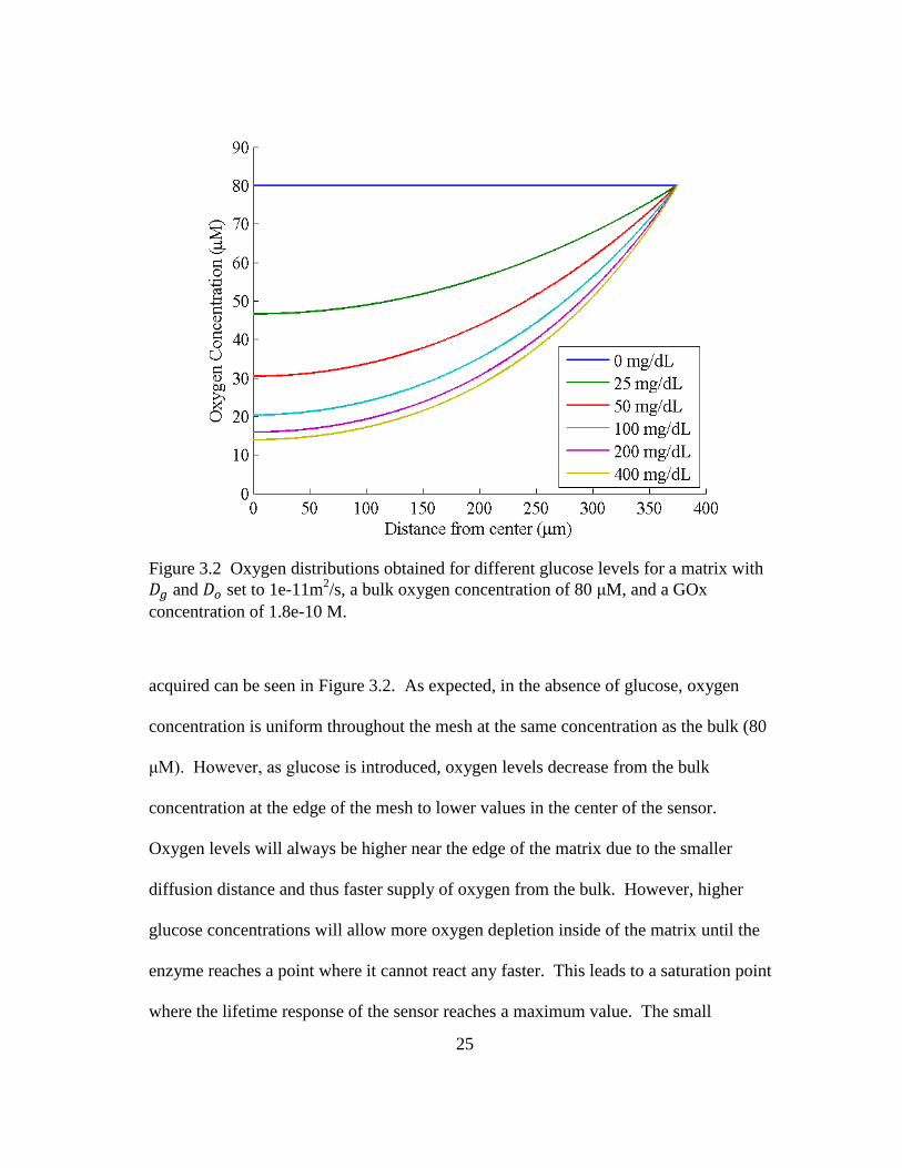
25
acquired can be seen in Figure 3.2. As expected, in the absence of glucose, oxygen
concentration is uniform throughout the mesh at the same concentration as the bulk (80
μM). However, as glucose is introduced, oxygen levels decrease from the bulk
concentration at the edge of the mesh to lower values in the center of the sensor.
Oxygen levels will always be higher near the edge of the matrix due to the smaller
diffusion distance and thus faster supply of oxygen from the bulk. However, higher
glucose concentrations will allow more oxygen depletion inside of the matrix until the
enzyme reaches a point where it cannot react any faster. This leads to a saturation point
where the lifetime response of the sensor reaches a maximum value. The small
Figure 3.2 Oxygen distributions obtained for different glucose levels for a matrix with
and set to 1e-11m2/s, a bulk oxygen concentration of 80 μM, and a GOx
concentration of 1.8e-10 M.

26
difference in the oxygen distribution from 200 to 400 mg/dL shows that the response of
this sensor is near the saturation point at these glucose levels. Although not depicted,
under the appropriate conditions (faster glucose diffusion, higher GOx concentrations,
and slower oxygen diffusion) oxygen levels can be depleted within the sensor matrix.
As mentioned above, luminescent enzymatic glucose sensors can utilize an
oxygen sensitive dye to measure the glucose response. The luminescent response, i.e.
lifetime, is related to oxygen concentration through the Stern-Volmer relationship:
[ ]
3.4
where is the lifetime in the absence of oxygen, is the lifetime, is the Stern-
Volmer constant, and [ ] is the oxygen concentration.149
The Stern-Volmer properties
utilized in this study were determined after measuring the response of a hydrogel sensor
in vitro. Experimental details and results can be found in the following section.
To further characterize the modeled sensor response, the Thiele modulus was
utilized. This parameter is often used to describe the reaction-diffusion properties of an
enzymatic system.14, 16, 36, 150-151
For glucose, the Thiele modulus is calculated using:
√ [ ]
[ ] 3.5
where is the catalytic turnover rate ( in Equation 3.1), [ ] is the concentration
of GOx, is the diffusion coefficient for glucose, [ ] is the bulk glucose concentration,
and is the length of the matrix .16
For this study, the glucose concentration was set to
400 mg/dL, the maximum concentration modeled, for all calculations. Inspection of

27
Equation 3.5 reveals that the numerator represents the maximum rate of substrate
conversion while the denominator represents the maximum rate of substrate transport.150
Thus high values for the Thiele modulus (typically > 1) indicate the system is diffusion-
limited, whereas low values (< 0.3) indicate a reaction-limited system.15, 123, 151
A Thiele
modulus can also be calculated for oxygen in a similar manner:
√ [ ]
[ ] 3.6
where is the diffusion coefficient for oxygen, and [ ] is the ambient oxygen
concentration. A value of 80 μM was utilized for all calculations. The ratio of the
Thiele moduli for oxygen and glucose is also of interest for oxygen-dependence studies.
This allowed the investigation of oxygen-dependence in relation to the relative
diffusional properties of the system. This ratio can be determined by:
√
[ ]
[ ] 3.7
where the catalytic turnover rate, GOx concentration, and matrix length from the original
moduli cancel out, leaving contributions only from the relative concentrations and
diffusivity of the two substrates.
3.2 Oxygen Response Measurements of a Hydrogel Sensor
Although and will change from material-to-material due to diffusion
properties,149
the change in sensitivity to oxygen is expected to be minimal compared to
dependence on enzymatic reaction rate and diffusion properties. Thus, to simplify

28
modeling and reduce the number of in vitro experiments, single values for and
were utilized for all cases.
The values utilized for these parameters were determined for a sensor similar to
one previously reported.30
To make this hydrogel, a solution was made by combining 2-
hydroxyethylmethacrylate (HEMA, Polysciences, Inc.) and tetraethylene glycol
dimethacrylate (Polysciences, Inc.) in a molar ratio of 98:2. Then 250 μL of this
solution was mixed with 2.5 mg of the photoinitiator 2,2-Dimethoxy-2-phenyl-
acetophenone (Aldrich). This was followed by additions of 100 μL of ethylene glycol
(Sigma), 47.5 μL of de-ionized water, 100 μL of 5 mM tetramethacrylated palladium
porphyrin dissolved in dimethyl sulfoxide (Sigma). The porphyrin was synthesized
using Pd(II) meso-Tetra(4-carboxyphenyl)porphine (Frontier Scientific) as a base.*
After mixing, the solution was added to a mold made by an 0.03” Teflon spacer placed
between two glass slides. The solution was then vacuumed to remove any bubbles and
UV polymerized for 5 minutes on each side. The resulting pHEMA hydrogel was placed
in a solution of dichloromethane for 24 hours and then rinsed with acetone. The gels
were then stored in a solution of 0.01 M phosphate buffered saline (PBS) until testing
was performed.
The response of the sensor was tested by removing a sample from the gel using a
2.5 mm biopsy punch. The sample was then immobilized in a custom reaction chamber
previously reported and the luminescence lifetime response to varying oxygen was
determined.152-153
The oxygen concentration was controlled by varying the flow rate of
* The methacrylated form of this dye was synthesized and graciously provided by Dr. Soya Gamsey of
Profusa, Inc.

29
oxygen into a PBS solution. Chapters 5 as well as the appendices contain further details
about the testing and measurement system utilized. The raw data were then analyzed
using MATLAB (MathWorks, Inc.) to determine the oxygen response which can be seen
in Figure 3.3. As expected, the sensor showed a higher sensitivity to oxygen at low
concentrations. The Stern-Volmer quenching curve shown in the inset was fit using
linear regression to determine . The values of and used for modeling were
0.104 μM-1
and 675 μs, respectively.
Figure 3.3 The lifetime response of an oxygen-sensitive palladium porphyrin
immobilized in pHEMA. The inset shows the resulting Stern-Volmer plot. Error bars
represent standard deviation with n = 10.

30
3.3 Results and Discussion
3.3.1 Modeled Glucose Sensor Response
Initially sensor responses were modeled using a range of diffusion coefficients
for glucose and oxygen based on reported values for hydrogels (Table 3.1). Three
values were chosen for each diffusion coefficient, representing a total of nine unique
materials with different diffusional properties, and, hence, different Thiele moduli.
Enzyme concentration was also varied by selecting different values for (0.1, 0.5, 1, 5,
10, and 50). The response curves obtained for the range of values can be seen in
Figure 3.4. Each graph also shows the results of different values tested; repeated
values are due to the ratio of the diffusion coefficients tested (see above). There was
very little response seen when was less than 1, as expected. However, for response
where was 1 or larger and when is 2 or less, the response of the sensor was also
very low. When is very large (>100), the response becomes saturated at very low
glucose concentrations (<25 mg/dL) which was observed for all ≥ 1. These results
indicate that provided enough GOx, there is a “sweet spot” for that would yield a
desirable combination of high sensitivity and response over a wide range of
concentrations before saturation is reached. Based on these results, diffusion
coefficients for glucose and oxygen were both set to 1e-11 m2/s so that a suitable range
and sensitivity could be produced. Interestingly, these values are close to the reported
values of pHEMA (Table 3.1).
In order to have a sensor with suitable response (i.e. range and sensitivity),
needs to be between 2 and 100 (Figure 3.4). When is 16.7, the GOx concentration

31
Figure 3.4 Representative glucose responses for a range of oxygen and glucose
diffusion coefficients (represented in ratio form) as well as a range of values.

32
plays more of a role in sensor response as seen in Figure 3.5. Using these diffusion
coefficients, the lifetime response for different GOx concentrations was plotted versus
glucose concentration and fit using:
[ ]
⁄ 3.8
where , , and are fit parameters. This was equation was chosen for the calibration
curve because it showed a high goodness of fit (R2) with the data evaluated. It should be
noted that any equation can be utilized for calibration purposes (i.e. if the response
profile follows a different shape) as long as a high quality of fit can be obtained allowing
accurate predictions of glucose or other analytes. However, for compensation purposes
Figure 3.5 Modeled response of a sensor using different GOx concentrations and with
and set to 1e-11m2/s and a bulk oxygen concentration of 80 μM.

33
where the fit parameters will be determined as a function of the interfering analyte, an
equation with fewer fit parameters is desired in order to reduce overall complexity of the
calibration. This led to the selection of Equation 3.8 for calibration because only three
fit parameters were required to obtain a high quality of fit.
Due to the exponential nature of Equation 3.8, parameter is representative of
the percent change of the signal while is representative of the range and sensitivity. As
expected, the values for and obtained after fitting the data in Figure 3.5 are inversely
related for different GOx concentrations (Figure 3.6). As decreases, the range will
decrease but the sensitivity will increase and vice versa.
Figure 3.6 Plots of the values obtained for parameters and versus transformed GOx
concentrations. Parameters were obtained by fitting the results in Figure 3.5. The black
line in each graph represents the optimal GOx concentration for a range of 200 mg/dL.
34
To allow easier fitting of and , the GOx concentration was transformed
logarithmically and through shifting ( ([ ]) ( ([ ]))). Fitting
was performed using:
3.9
where is either or , is the transformed GOx concentration, and , , and are
fit parameters. Fitting of the parameters using this equation allowed the trends in the
range and sensitivity to be determined for a wide range of GOx concentrations. By
defining the range as the point at which 90% of the exponential has decayed, the optimal
value for can be found using:
Figure 3.7 This graph shows the oxygen dependent response for three different model
materials at four different oxygen concentrations.

35
( ⁄ )
3.10
where is the desired range and is the percentage (90%). Once is known, the
appropriate GOx concentration can be found using the fits for Equation 3.9. For a
desired range of 200 mg/dL, the optimal GOx concentration was found to be 1.62e-10 M
using Equation 3.10.
3.3.2 Oxygen Dependent Response of Enzymatic, Glucose Sensors
After finding the appropriate GOx concentration (1.62e-10 M) and diffusion
coefficients ( = = 1e-11 m2/s), further sensor response modeling was performed for a
range of oxygen concentrations. A range of oxygen diffusion coefficients (1e-13, 1e-11,
and 1e-9 m2/s) was again used to see if would influence the response’s dependency
on oxygen. The results obtained can be found in Figure 3.7. For low values of (1e-
13 m2/s) and high values of (167), the response saturates at very low glucose
concentration indicating a low range. At a higher value of (1e-9 m2/s) or lower
values of (1.67), the range is much higher, but the sensitivity is too low. When
and are equal ( = 16.7), however, the response is improved because it shows
suitable range and sensitivity, similar to the results seen in Figure 3.5.
Based on analysis of the previous data, a more extensive oxygen-dependence
study was performed for a sensor with = = 1e-11 m2/s and a GOx concentration of
1.62e-10 M. This was done by modeling the sensor response for a higher resolution
within the already specified range of glucose and oxygen concentrations (Figure 3.8).
After modeling, the responses were again fit using Equation 3.8. Fits were performed

36
for glucose values ranging from 40 to 400 mg/dL in order to increase the accuracy of the
fit ( > 0.99). It is assumed that using only the values above 40 mg/dL for the fitting is
acceptable, as lower values will not affect the clinical treatment (i.e. sugar intake) for
low glucose concentrations.154
The trends in the fit parameters were investigated by plotting them versus oxygen
concentration and fitting them using a 4th
order polynomial (
). The complexity of this fit was required in order to ensure a high quality of
fit ( ≥ 0.9999) for the calibration curves. The resulting fits of the data in Figure 3.8
Figure 3.8 This graph shows the modeled sensor response for = = 1e-11 m2/s,
[GOx]=1.62e-10 M, and a range of oxygen concentrations. The dashed lines represent
the fitting of the data for glucose values from 40 to 400 mg/dL.

37
using the parameter values obtained from Figure 3.9 showed good agreement with the
data in Figure 3.8 ( > 0.98).
The data in Figure 3.8 were then used to perform preliminary oxygen
compensation tests by comparing the predicted glucose values with the actual values.
To determine the predicted glucose levels, Equation 3.8 was solved for the glucose
concentration and the lifetime values from Figure 3.8 and the appropriate parameters for
, , and obtained from the fits in Figure 3.9 were inserted. These predictions were
also compared with uncompensated glucose predictions using the calibration curve
obtained for 80 μM oxygen which is in the middle of the oxygen range tested.
Figure 3.9 Fit parameters of Equation 3.8 as functions of oxygen concentration. Blue
circles show actual values obtained and dashed lines represent the fit.
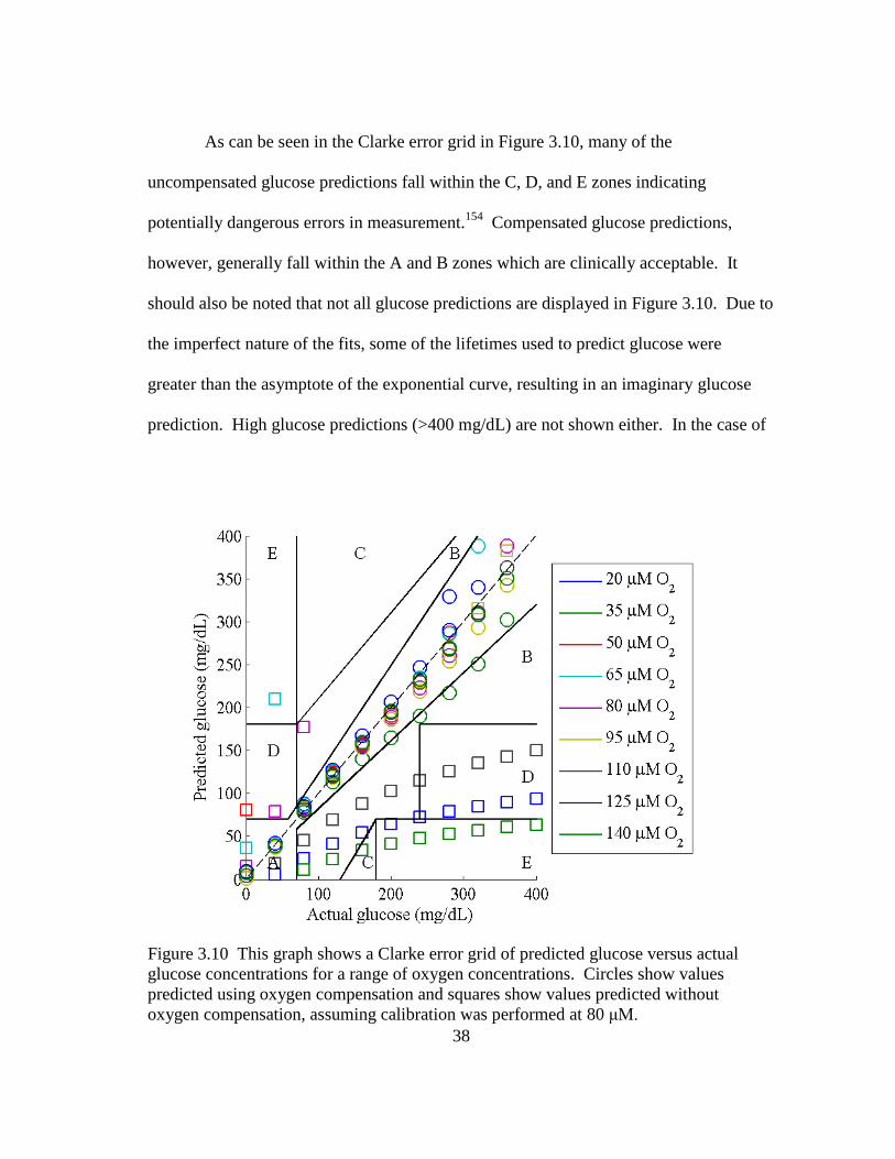
38
As can be seen in the Clarke error grid in Figure 3.10, many of the
uncompensated glucose predictions fall within the C, D, and E zones indicating
potentially dangerous errors in measurement.154
Compensated glucose predictions,
however, generally fall within the A and B zones which are clinically acceptable. It
should also be noted that not all glucose predictions are displayed in Figure 3.10. Due to
the imperfect nature of the fits, some of the lifetimes used to predict glucose were
greater than the asymptote of the exponential curve, resulting in an imaginary glucose
prediction. High glucose predictions (>400 mg/dL) are not shown either. In the case of
Figure 3.10 This graph shows a Clarke error grid of predicted glucose versus actual
glucose concentrations for a range of oxygen concentrations. Circles show values
predicted using oxygen compensation and squares show values predicted without
oxygen compensation, assuming calibration was performed at 80 μM.

39
oxygen compensated glucose predictions, these predictions (high and imaginary)
occurred at higher glucose levels (≥300 mg/dL) making it less clinically relevant.
Uncompensated glucose predictions, however, produced high and imaginary predictions
for the entire range of glucose values tested but this decreased as oxygen levels got
closer to 80 μM.
Negative glucose values can also be predicted because the glucose curves were
only fit from 40 to 400 mg/dL, however, this only occurred when the glucose level was
40 mg/dL or less. The clinical treatment in these cases would not change indicating that
this not likely an issue. The number of predictions that fall into each region for each
method can be found in Table 3.2. In order to assign a region to every prediction, the
lines of the grid were extended for negative and high (>400 mg/dL) predictions and
imaginary predictions were assumed to be 400 mg/dL. These results show that glucose
predictions without oxygen compensation are only relevant at oxygen concentrations
near the concentration at which the calibration was performed. These results indicate
that compensation is necessary in order to have a viable glucose prediction.
Table 3.2 Number of glucose predictions that fall within the respective regions for each
Clarke error grid displayed.
Figure 3.10 Figure 3.11 Figure 3.13
Region Uncomp. Comp. Uncomp. Comp. Uncomp. Comp.
A 33 94 10 99 22 77
B 12 4 38 0 23 20
C 31 1 44 0 48 1
D 10 0 2 1 2 2
E 13 0 6 0 5 0
% Clinically
Acceptable 45% 99% 46% 99% 45% 97%

40
In order to more fully test the viability and necessity of oxygen compensation
for enzymatic glucose sensors, 100 glucose predictions were made with and without
compensation. The glucose calibration curve obtained at 80 μM was again used for
uncompensated glucose predictions. Random concentrations were obtained using a
reported physiological glucose distribution (μ=133.3 and σ=72.1 mg/dL) and a uniform
oxygen distribution from 20 to 140 μM.146
As expected, Figure 3.11 shows that oxygen compensated glucose predictions
are much more accurate than predictions that do not consider the ambient oxygen level.
Figure 3.11 This Clarke error grid shows glucose predictions obtained from random
oxygen and glucose values. Theoretical measurement error is not included. Blue circles
show oxygen compensated predictions and red squares show uncompensated
predictions. Markers that are filled in represent negative or imaginary glucose
predictions (see text). It should be noted that these values only represent the presence of
an erroneous prediction and not an actual predicted glucose value.
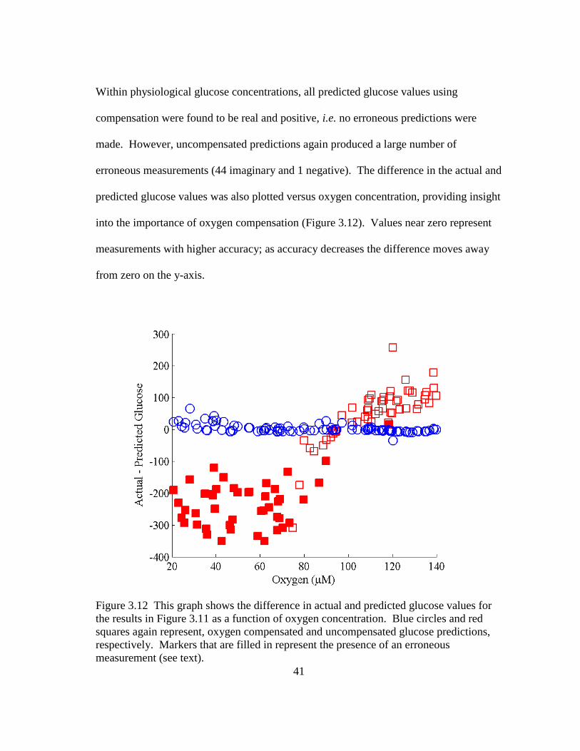
41
Within physiological glucose concentrations, all predicted glucose values using
compensation were found to be real and positive, i.e. no erroneous predictions were
made. However, uncompensated predictions again produced a large number of
erroneous measurements (44 imaginary and 1 negative). The difference in the actual and
predicted glucose values was also plotted versus oxygen concentration, providing insight
into the importance of oxygen compensation (Figure 3.12). Values near zero represent
measurements with higher accuracy; as accuracy decreases the difference moves away
from zero on the y-axis.
Figure 3.12 This graph shows the difference in actual and predicted glucose values for
the results in Figure 3.11 as a function of oxygen concentration. Blue circles and red
squares again represent, oxygen compensated and uncompensated glucose predictions,
respectively. Markers that are filled in represent the presence of an erroneous
measurement (see text).

42
Erroneous measurements were plotted by substituting 400 mg/dL for imaginary
glucose predictions and 0 mg/dL for negative glucose predictions. Compensated values
showed a near uniform variation across the range of oxygen concentrations with some
increase at lower oxygen concentrations which is most likely due to a loss in range at the
lower oxygen concentrations (Figure 3.8). The mean difference and standard deviation
for oxygen compensated measurements was 3.3 and 12.8 mg/dL, respectively.
Uncompensated values had a mean difference of -76.5 mg/dL and a standard deviation
of 163.1 mg/dL. Uncompensated glucose predictions showed a linear trend with the
highest accuracy occurring at 80 μM as expected. Predictions with less than 80 μM
oxygen tended to be imaginary due to the low percent change of that calibration curve
while predictions at higher oxygen concentrations showed a decreasing accuracy. It is
expected that if calibration was performed at another oxygen concentration, the results
would be similar where the highest accuracy should occur near the oxygen concentration
at which calibration was performed.
In a second test, theoretical measurement error was also introduced into the
system to see how this would affect in vivo glucose predictions. A pooled standard
deviation (0.61 μs) was determined using the lifetime results in Figure 3.3 and applied to
the lifetime response produced by the model. In addition, an equation for random
uncertainty was applied to the same results to obtain an oxygen measurement standard
deviation of 2.17 μM.155
When applied to the model, similar results were seen (Figure 3.13) when
measurement error was introduced into the system as those made without measurement

43
error. Glucose predictions did become less accurate for both cases but oxygen
compensated predictions again showed a higher accuracy than those made without
compensation. One erroneous prediction (1 negative value) was made for compensated
glucose predictions while 50 measurements (47 imaginary, 3 negative) were erroneous
for uncompensated predictions. The trends in accuracy as a function of oxygen
concentration also showed results similar to those in Figure 3.12 but with slightly lower
accuracy overall. The average difference and standard deviation for oxygen
Figure 3.13 This Clarke error grid shows glucose predictions obtained from random
oxygen and glucose values. Theoretical measurement error was also considered. Blue
circles show oxygen compensated predictions and red squares show uncompensated
predictions. Markers that are filled in represent negative or imaginary glucose
predictions (see text). It should be noted that these values only represent the presence of
an erroneous prediction and not an actual predicted glucose value.
44
compensated glucose predictions was -0.9 and 41.2 mg/dL, respectively.
Uncompensated predictions had a mean and standard deviation of -103.9 and 162.5
mg/dL, respectively.
3.4 Conclusions
The inaccuracy of enzymatic, glucose sensors due to variability in the ambient
oxygen concentration was demonstrated in silico. This is a major concern for in vivo
applications (i.e. self-monitoring of blood glucose levels) where oxygen levels are
expected to vary. To overcome this issue, a technique for compensation using an
oxygen dependent calibration curve was described where the appropriate calibration
curve was selected based on ambient oxygen concentration. Using this approach,
glucose predictions were found to be more accurate than uncompensated predictions
over a wide range of ambient oxygen concentrations. Despite the extensive calibration
that will be required in vitro before implementation in vivo, the improvement in accuracy
outweighs this drawback. This oxygen compensation technique addresses a limitation
of current enzymatic, glucose assays and could also be utilized to improve the accuracy
of other enzymatic assays.
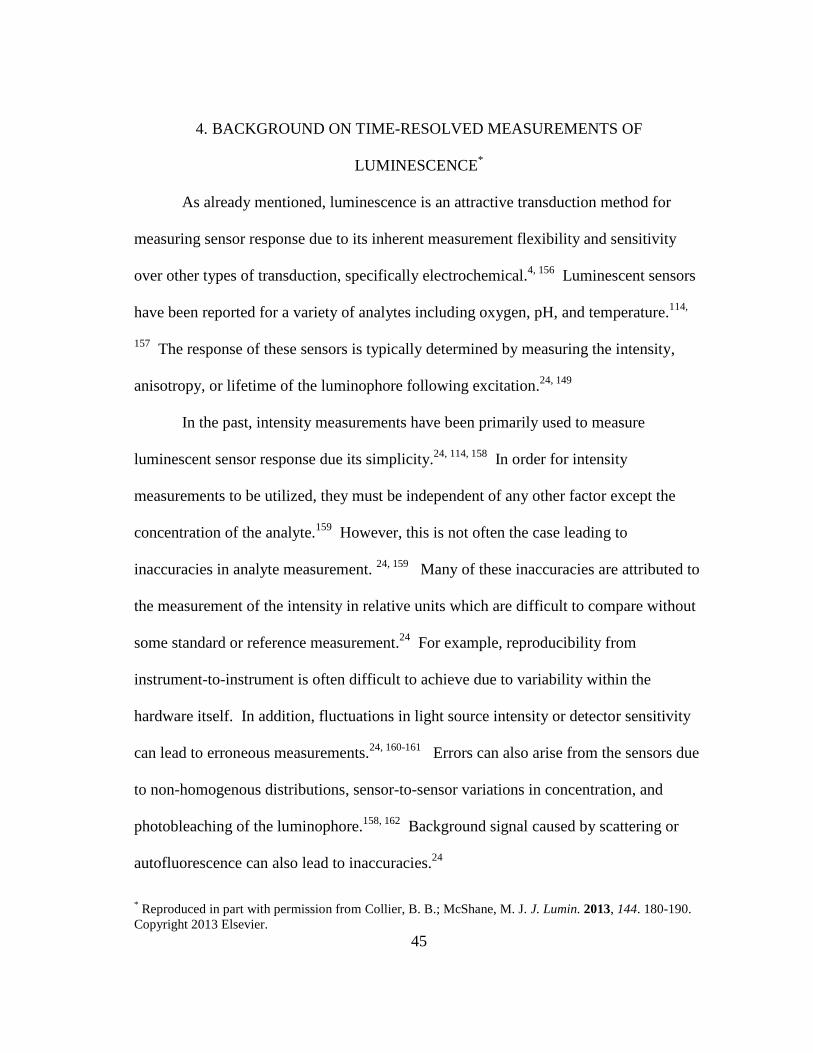
45
4. BACKGROUND ON TIME-RESOLVED MEASUREMENTS OF
LUMINESCENCE*
As already mentioned, luminescence is an attractive transduction method for
measuring sensor response due to its inherent measurement flexibility and sensitivity
over other types of transduction, specifically electrochemical.4, 156
Luminescent sensors
have been reported for a variety of analytes including oxygen, pH, and temperature.114,
157 The response of these sensors is typically determined by measuring the intensity,
anisotropy, or lifetime of the luminophore following excitation.24, 149
In the past, intensity measurements have been primarily used to measure
luminescent sensor response due its simplicity.24, 114, 158
In order for intensity
measurements to be utilized, they must be independent of any other factor except the
concentration of the analyte.159
However, this is not often the case leading to
inaccuracies in analyte measurement. 24, 159
Many of these inaccuracies are attributed to
the measurement of the intensity in relative units which are difficult to compare without
some standard or reference measurement.24
For example, reproducibility from
instrument-to-instrument is often difficult to achieve due to variability within the
hardware itself. In addition, fluctuations in light source intensity or detector sensitivity
can lead to erroneous measurements.24, 160-161
Errors can also arise from the sensors due
to non-homogenous distributions, sensor-to-sensor variations in concentration, and
photobleaching of the luminophore.158, 162
Background signal caused by scattering or
autofluorescence can also lead to inaccuracies.24
* Reproduced in part with permission from Collier, B. B.; McShane, M. J. J. Lumin. 2013, 144. 180-190.
Copyright 2013 Elsevier.

46
To reduce the instrument-related problems, several wavelength ratiometric
approaches have been developed.152, 163
These approaches either utilize a dual emitting
dye where the peaks respond in opposite directions (i.e. the intensity at one wavelength
increases while the other decreases) or two luminophores, one of which is an insensitive
reference (i.e. remains constant) and the other is sensitive to the desired analyte (Figure
4.1).164
Due to the self-referencing nature of these kinds of sensors, the results are
generally more reproducible from instrument-to-instrument.24
However, photo-
bleaching is still a concern for two luminophore systems because the time-dependent
rate can be different for each luminophore utilized.24
Thus if one luminophore bleaches
faster than the other luminophore, drifts in the ratiometric response will occur.
Temperature-dependent quenching will also be different for each luminophore again
leading to a drift in the response as the ambient temperature changes.24
In addition, the
Figure 4.1 A) Diagram of an intensity-based ratiometric response where P1 is the peak of
an insensitive reference and P2 is the analyte sensitive luminophore. B) Another
intensity-based ratiometric response where both P1 and P2 respond to the analyte of
interest but in opposite directions.
47
sensor-related issues discussed above (e.g. variations in concentration from sensor-to-
sensor) will remain an issue with ratiometric systems utilizing two luminophores.
Although this is less of an issue for dual-emitting or self-referencing luminophores,
luminophores with the appropriate spectral and sensing properties may not be available.
Measurements of luminescence anisotropy can also be utilized by exciting a
luminophore with polarized light.24, 149
Analyte-dependent rotational diffusion of the
luminophore allows measurements of the degree of polarization or anisotropy to be used
for sensing applications.24
Anisotropy can overcome some of the issues of intensity
measurements; however, this technique is still susceptible to inaccuracies due to
scattering and any diffusional restriction (e.g. rigid immobilization) of the dye will lead
to a loss in sensitivity.24
Measurements of the luminescence decay rate or lifetime are of interest because
they are not susceptible to the errors that hinder intensity and anisotropy
measurements.24
This is because the lifetime response if independent of the
luminophore concentration and not sensitive to the optical parameters of the
instrumentation.24
In addition, background signal due to scattering or auto-fluorescence
is often not an issue because these events are present for only a few nanoseconds while
most luminescent indicators have longer lifetimes (tens of nanoseconds to greater than a
millisecond).24
Lifetime measurements can either be made in the time-domain (TD)
with pulsed excitation light or in the frequency-domain (FD) with intensity-modulated
light. TD-based approaches are attractive for in vivo measurements because they are less
affected by short-lived scattered excitation light or tissue autofluorescence than FD

48
measurements. These background signals can be removed in the FD also, but require
measurement at multiple frequencies which is time consuming.149, 165-166
In addition, the long lifetimes of the luminophores utilized for oxygen and
glucose sensing allow luminescence decays to be recorded in a single measurement
rather than re-built using time-correlated single photon counting TCSPC which is often
used for imaging applications.149, 161
The long lifetimes also prevent the need for
deconvolution of the luminescence from the excitation signal or any instrument
response.
Some of the more applicable lifetime calculation techniques will be discussed
below, but further review of other lifetime calculation techniques for mono- and dual-
exponential decays can also be found elsewhere.149, 165, 167
4.1 Numerical Analysis
The lifetime of a mono-exponential decay can be calculated using a variety of
methods including linear and non-linear least squares analysis (LLS and NLLS,
respectively), the phase-plane method (PPM), the maximum likelihood estimator (MLE),
the maximum entropy method (MEM) and the rapid lifetime determination (RLD)
method.149, 167-170
Of these methods, NLLS is most often utilized but relies on several
assumptions and can require extensive computational power making it unsuitable for
real-time applications.25, 149, 171-173
In addition, NLLS does not guarantee a suitable
solution for the lifetime which can be dependent on the initial guess of the parameters
for the fit.25, 173
Accuracy can be improved by using weighted least-squares analysis
whereby data points with lower standard deviation are given higher priority towards
49
fitting which is often done in cases where the standard deviation across the data set is
variable but in a predictable manner.174
However, when using a weighted approach, it is
often assumed that the weights are known exactly which is usually not the case. If the
data are improperly weighted, inaccuracies can occur.175-176
A closed form solution for
the lifetime can also be obtained by transforming the data logarithmically (after
background subtraction) and using LLS analysis.27, 173
Usually only a portion of the
decay is analyzed after logarithmic transformation because errors can occur due to
inaccurate baseline levels.29, 177
Weighting of the response is typically utilized with this
method which again must be chosen carefully.178-179
Lifetime calculations using the
Guggenheim method eliminate the need for background correction by plotting the
logarithmic transform of the difference between equally-spaced, paired data points.177
This and other numerical analysis techniques have given way to NLLS analysis,
however.
More recently developed techniques tend to utilize window integration to
perform lifetime calculation. This is done by dividing the decay data into separate bins
or windows which are then summed.171, 180
Integration can also be performed in real-
time using CCD cameras.181
Different methods utilizing window integration are
discussed below.
4.2 Phase-Plane Method
The Phase-Plane Method (PPM) developed earlier by Demas et al. was one of
the earliest methods to utilize window integration to calculate lifetimes.182
This
approach transforms data obtained using windows and determines the lifetime by finding
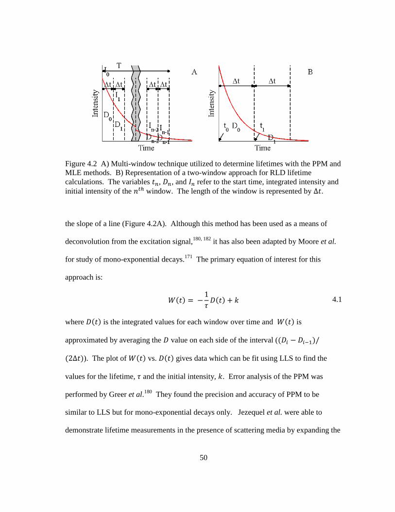
50
the slope of a line (Figure 4.2A). Although this method has been used as a means of
deconvolution from the excitation signal,180, 182
it has also been adapted by Moore et al.
for study of mono-exponential decays.171
The primary equation of interest for this
approach is:
( )
( ) 4.1
where ( ) is the integrated values for each window over time and ( ) is
approximated by averaging the value on each side of the interval (( )
( )). The plot of ( ) vs. ( ) gives data which can be fit using LLS to find the
values for the lifetime, and the initial intensity, . Error analysis of the PPM was
performed by Greer et al.180
They found the precision and accuracy of PPM to be
similar to LLS but for mono-exponential decays only. Jezequel et al. were able to
demonstrate lifetime measurements in the presence of scattering media by expanding the
Figure 4.2 A) Multi-window technique utilized to determine lifetimes with the PPM and
MLE methods. B) Representation of a two-window approach for RLD lifetime
calculations. The variables , , and refer to the start time, integrated intensity and
initial intensity of the window. The length of the window is represented by .
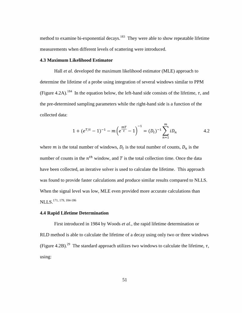
51
method to examine bi-exponential decays.183
They were able to show repeatable lifetime
measurements when different levels of scattering were introduced.
4.3 Maximum Likelihood Estimator
Hall et al. developed the maximum likelihood estimator (MLE) approach to
determine the lifetime of a probe using integration of several windows similar to PPM
(Figure 4.2A).184
In the equation below, the left-hand side consists of the lifetime, , and
the pre-determined sampling parameters while the right-hand side is a function of the
collected data:
( ) ( )
( ) ∑
4.2
where is the total number of windows, is the total number of counts, is the
number of counts in the window, and is the total collection time. Once the data
have been collected, an iterative solver is used to calculate the lifetime. This approach
was found to provide faster calculations and produce similar results compared to NLLS.
When the signal level was low, MLE even provided more accurate calculations than
NLLS.171, 179, 184-186
4.4 Rapid Lifetime Determination
First introduced in 1984 by Woods et al., the rapid lifetime determination or
RLD method is able to calculate the lifetime of a decay using only two or three windows
(Figure 4.2B).29
The standard approach utilizes two windows to calculate the lifetime, ,
using:
52
( ) 4.3
where is the window length, and is the integrated intensities for the
window.27
If the background level is unknown and nonzero, a third window may be
incorporated into the calculation.28-29
Because iterative approaches are not utilized, this
method is significantly faster than LS analysis, allowing real-time sampling of the
luminophore lifetime.27, 29
However, the accuracy of the lifetime calculation has been
shown to be dependent on the length of the window with respect to the lifetime.27, 187
Waters et al. developed a method to determine the optimal window length based on the
mean expected lifetime for a dynamically changing luminophore to reduce the effects of
this problem.188
Sharman et al. also determined that overlapping the windows improves
accuracy of the calculation.181
Collier and McShane recently demonstrated a method that
utilizes windows with dynamically changing lengths; compared to the static window
lengths previously used. This real-time adjustment of windows leads to improved
lifetime accuracies over a wide range of lifetime values.153
Following the development of RLD, several iterative approaches utilizing two
windows have also been developed. Rather than implement both windows following the
end of excitation, Chan et al. developed the Square-Wave RLD (SWRLD) method
which applies one window during the excitation of the luminophore and one
immediately following.187
They found the precision of this method comparable NLLS
and superior to the standard RLD approach. Chan et al. also developed a generalized
RLD (GRLD) approach that utilizes two overlapping windows of unequal length
implemented following probe excitation.189
Again, this method showed improved

53
accuracy over standard RLD calculations. Both of these methods, however, require an
iterative solver which leads to increased computation time compared to RLD.153
Moore et al. compared several of these window-based approached and found the
precision of MLE, PPM, and GRLD was much better than standard RLD.171
They also
showed that PPM is susceptible to systematic errors at large sampling times which can
be reduced by increasing the number of windows used. MLE was found to have
consistently lower standard deviations than the other methods; however, both MLE and
RLD were susceptible to errors due to non-zero baselines.
4.5 Dual-Exponential Lifetime Decay Response Measurement Techniques
Much like single sensor responses, NLLS is often used to calculate lifetimes
when multiple emitters are present; in this case, multi-exponential fits are applied
(similar to equation 12). In addition, the luminescence acquisition method required for
multi-exponential response in the TD is often not different than the method used for
mono-exponential responses, making them easier to implement than multi-luminophore
FD approaches. However, in order to distinguish the lifetimes of multiple luminophores,
they need to be temporally-distinct.181
Hradil et al. developed one of the first methods to utilize temporally-distinct
luminophores for dual lifetime calculations that does not require multi-exponential LS
analysis.190
This method was utilized for temperature compensation of an oxygen
sensing film. In order to resolve the response of both luminophores, the decay time of
the longer-lived luminophore is approximately three orders of magnitude longer than the
other luminophore (Figure 4.3). This is necessary in the TD in order to ensure the

54
contribution from is constant while measuring the response of and while measuring
the response of , the response of has decayed to zero. The response of the longer-
lived luminophore is sampled after a delay to prevent any contamination from the
shorter-lived luminophore. NLLS is then used to determine each lifetime.
In addition to NLLS, the RLD approach has been also been expanded for multi-
exponential decay calculations by Sharman et al.181
Similar to RLD for mono-
exponential decays, two windows for each luminophore are used and are applied either
contiguously or overlapping (Figure 4.4). The ratio of the to for this approach,
Figure 4.3 Depiction of TD decays for two temporally-distinct dyes with lifetimes of 5
and 1,000 μs. Inset is of the same decays but at a smaller period to show the decay of
the shorter-lived luminophore and the nearly constant signal of the longer-lived
luminophore.

55
however, needs to be at least 2; the precision of the measurement is reduced as the
lifetimes get closer.181
The calculations for this dual RLD approach, however, are more
complicated than the traditional RLD calculation and the method seems to be susceptible
to measurement noise.191
Another method that utilizes the principles of RLD is the Dual Lifetime
Determination (DLD) method developed by Nagl et al.156, 162, 192
Similar to the scheme
used by Hradil, the probes must be temporally-distinct; however, this method utilizes the
standard RLD calculation to determine the lifetime rather than NLLS. Two pairs of
windows are required (one for each lifetime calculation), where the second pair is
Figure 4.4 Example of a contiguous, equi-width window implementation of dual RLD
lifetime calculations.
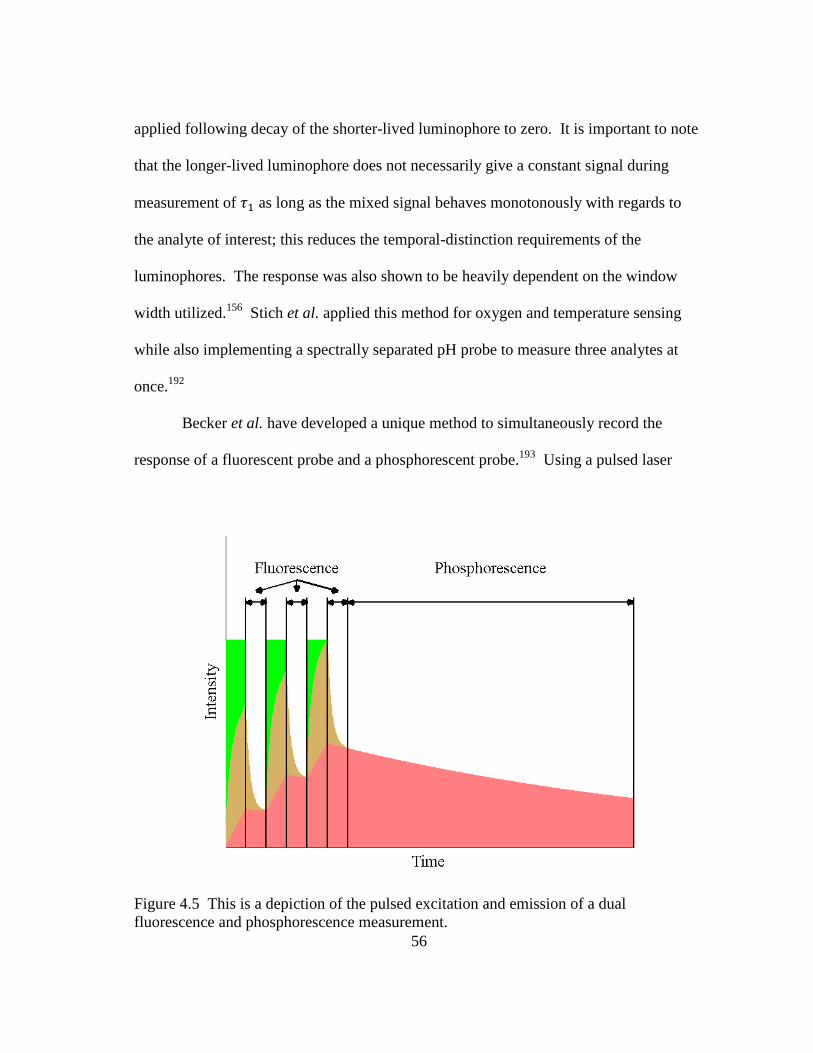
56
applied following decay of the shorter-lived luminophore to zero. It is important to note
that the longer-lived luminophore does not necessarily give a constant signal during
measurement of as long as the mixed signal behaves monotonously with regards to
the analyte of interest; this reduces the temporal-distinction requirements of the
luminophores. The response was also shown to be heavily dependent on the window
width utilized.156
Stich et al. applied this method for oxygen and temperature sensing
while also implementing a spectrally separated pH probe to measure three analytes at
once.192
Becker et al. have developed a unique method to simultaneously record the
response of a fluorescent probe and a phosphorescent probe.193
Using a pulsed laser
Figure 4.5 This is a depiction of the pulsed excitation and emission of a dual
fluorescence and phosphorescence measurement.
57
with a high repetition rate, they were able to excite both probes simultaneously (Figure
4.5). Between excitation pulses of a pulse train, fluorescence decay measurements are
made (again assuming constant signal from the phosphor). During the pulse train,
however, phosphorescence steadily builds up due to its long decay time. After
completion of the pulse train, phosphorescence measurements are made. Lifetime
calculations are then made using NLLS.

58
5. DYNAMIC RAPID LIFETIME DETERMINATION*
Luminescent sensing and characterization have become widely researched areas
in biomedical, environmental and food industries because of their ability to provide
greater sensitivity and measurement flexibility when compared to electrochemical
analysis schemes.4, 156
In the past, intensity measurements have been predominantly
used to measure analyte concentrations or physical properties; however, these methods
are susceptible to many sources of error including photobleaching, drift in light source
intensity, and variations in dye concentrations from sensor to sensor.156, 194
These issues
can be overcome by measuring the rate of luminescence decay or lifetime which is
independent of the intensity (see Chapter 4 for more details).195-196
Although lifetime measurements can be made using either time-domain or
frequency-domain techniques, the former can be advantageous because of its ability to
easily eliminate scattering and shorter lifetime fluorescence from calculations. For
example, many proteins found in the body, including collagen and elastin, are known to
emit nanosecond lifetimes which can effect lifetime calculations of the dye. In addition,
time-domain methods have been shown to have a higher precision than frequency-
domain methods especially at lower intensities.195, 197
Traditionally, linear and non-
linear least-squares fittings have been used to determine the lifetime during time-domain
measurements but these methods require extensive computing power due to the large
number of iterations required to arrive at an accurate estimate.25, 173
The lifetimes
calculated with fittings are also dependent on the initial guesses for each parameter.25
If
* Reproduced with permission from Collier, B. B.; McShane, M. J. Anal. Chem. 2012, 84. 4725-4731.
Copyright 2012 American Chemical Society.
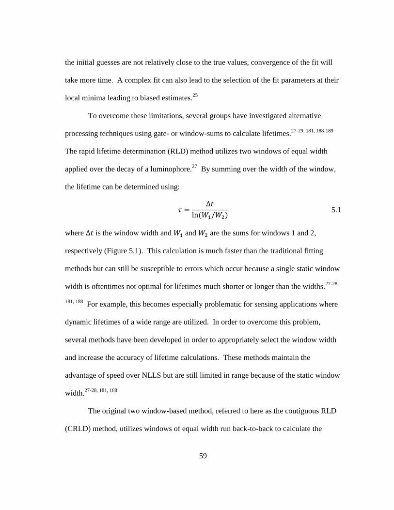
59
the initial guesses are not relatively close to the true values, convergence of the fit will
take more time. A complex fit can also lead to the selection of the fit parameters at their
local minima leading to biased estimates.25
To overcome these limitations, several groups have investigated alternative
processing techniques using gate- or window-sums to calculate lifetimes.27-29, 181, 188-189
The rapid lifetime determination (RLD) method utilizes two windows of equal width
applied over the decay of a luminophore.27
By summing over the width of the window,
the lifetime can be determined using:
( ) 5.1
where is the window width and and are the sums for windows 1 and 2,
respectively (Figure 5.1). This calculation is much faster than the traditional fitting
methods but can still be susceptible to errors which occur because a single static window
width is oftentimes not optimal for lifetimes much shorter or longer than the widths.27-28,
181, 188 For example, this becomes especially problematic for sensing applications where
dynamic lifetimes of a wide range are utilized. In order to overcome this problem,
several methods have been developed in order to appropriately select the window width
and increase the accuracy of lifetime calculations. These methods maintain the
advantage of speed over NLLS but are still limited in range because of the static window
width.27-28, 181, 188
The original two window-based method, referred to here as the contiguous RLD
(CRLD) method, utilizes windows of equal width run back-to-back to calculate the
60
lifetime.27
The second window of the overlapping RLD (ORLD) method, however,
begins before the first one ends.181
Both of these methods utilize Eqn. 1 to calculate the
lifetime. However, the generalized RLD (GRLD) method, utilizes overlapping windows
of different width which requires a different equation to the calculate lifetime.189
For the current work, rather than use a window with a static width, a computer-
based algorithm to dynamically determine the appropriate window width is evaluated.
After collecting the data, I hypothesize the lifetime response will then be calculated with
increased accuracy compared to those methods with a static window width. In practice
this method will only be limited by the sampling frequency and the number of data
Figure 5.1 Diagram of the basic RLD lifetime determination approach with contiguous
windows of equal width.

61
points recorded over time, but in theory this method could calculate the lifetime of any
response. As with NLLS, however, a larger range of possible lifetimes will lead to an
increased number of iterations performed and increased computation time. This
approach is based on the original two-window RLD where the windows are contiguous
and of equal width, but will be applicable to a much more extensive range because the
window widths are allowed to change dynamically as the lifetime changes.
5.1 Theory
The optimal window width for lifetime determination is usually described by the
ratio of the window width, , to the lifetime, .27-28, 181, 189 Ballew and Demas initially
proposed an optimal ratio for contiguous RLD near and other groups later
describe an optimal region from 1 to 3 .27, 181, 189 To implement DRLD, the ratio of
window-sums can be correlated to by re-arranging Eqn. 1:
5.2
where is the ratio of the window-sums. The optimal range for can then be
plugged into this equation to get the corresponding optimal range for . When
performing the calculation for data that exhibit significant changes in , the window
widths should be adjusted for every lifetime calculation until is within the optimal
range or another termination condition is met.
To implement a dynamic window change, the window width can be adjusted by
multiplying the previously calculated lifetime by a value that lies in the middle of the
chosen optimal range of . The window size is initially set to a small value so that a

62
maximum window change is only used for increases in window width. Maximum
window widths and maximum window changes are also implemented to prevent
programming errors. Protection from negative values, which can occur when the
decay shows low signal-to-noise ratio, should also be implemented in this algorithm.
The lifetime is re-calculated until is in the optimal range, the maximum width is
reached, or a maximum number of loops has been reached. A flow-chart of the entire
algorithm can be seen in Figure 5.2 and an example of the code can be found in
Appendix C.
Figure 5.2 Simplified low chart of dynamic windowing algorithm operation.
63
5.2 Experimental Details
5.2.1 Lifetime Techniques
In addition to DRLD and NLLS, the three other static windowing methods
described previously were used for comparison of lifetime calculations. The width of
the windows for CRLD was set to which was previously determined to be the
optimal width for this method where is the mean expected lifetime.188
Two variations
of the ORLD method were utilized to calculate the lifetime. Both utilize a second
window start time of but the window widths were to set to 0.5 and 1 for ORLD1
and ORLD2, respectively. For GRLD, the equation below was adapted from the original
equation to incorporate an initial delay of the window start times:
( ) ( )
( ) 5.3
where is the fractional delay of in terms of , is the fractional delay of
(relative to ) in terms of , and is the width of in multiples of . Using an
iterative solver, is solved for and then plugged into:
5.4
to obtain a lifetime. The width of or was set to because an optimal value
was not previously determined. Other iterative window-summing methods for lifetime
calculation are available but often require 10 or more windows. This number of
windows means greater complexity and increased computation. These methods will not
be compared here but have been elsewhere.171, 185-186
For calculations performed, an
initial delay of window start times was set to 0.8 μs in order to eliminate back-scattered

64
excitation light from the lifetime calculations. This delay represents a single data point
collected for each decay (based on the sampling rate) and will not affect lifetime
calculations or optimal window widths. Theoretical implementation of each of these
methods can be seen in Figure 5.3.
5.2.2 Modeled Lifetime Responses
Initial modeling investigated the possible calculation errors in static window
width methods. If a dynamic windowing algorithm is not used and the lifetime response
changes dramatically, a large error may be observed. From our calculations, if the
Figure 5.3 Theoretical implementation over three different lifetimes of the four static
window methods utilized to compare to DRLD. is represented by a light colored box
and is represented by a dark colored box. Any overlap of the windows is represented
by a shade in between the two window colors.

65
lifetime response was 25 μs and the windows were 37.6 μs ( = 1.5) the calculated
lifetimes would have a very good accuracy and repeatability as indicated by a mean
modeled lifetime calculation of 24.8 μs and a standard deviation of 0.322 μs (n = 10,
SNR = 10). However, if the lifetime were to suddenly change to 250 μs, the precision of
the measurement is greatly reduced as seen by modeled calculations with a mean
lifetime of 264.2 μs and a standard deviation of 39.2 μs (n = 10, SNR = 10).
To test the algorithm described above, a lifetime profile was designed in
MATLAB (Mathworks, Inc.) to simulate a real-time response and test the ability of
different window-summing lifetime calculation methods to calculate a range of lifetimes.
A decay for each lifetime was simulated with a SNR of 10 (Figure 5.4), and each of the
five methods were used to calculate . The residuals and R2 values for each method
were also calculated to determine the accuracy of each method.
5.2.3 Custom Lifetime Measurement System
A custom time-domain lifetime measurement system was developed to
experimentally demonstrate the DRLD technique. For luminophore excitation, a fiber
optic green LED (530 nm peak, Industrial Fiber Optics, Tempe, AZ) was utilized with a
driver circuit (see Appendix A) to improve the operating speed (ns rise and fall times) of
the diode. The circuit consisted of a transistor and resistors and capacitors.
Luminescence detection was performed using an avalanche photodiode module (APD,
C5460, Hamamatsu). Two plano-convex lenses (LA1951-A, Thor Labs) were used to
collect the luminescence from a bifurcated fiber bundle and focus it onto the active area
of the APD. A long-pass filter (3RD620LP, Omega Optical) was also used to reduce

66
interference from back-scattered excitation light. A data acquisition board (USB-6259,
National Instruments) was used to provide an excitation signal to the LED and collect
the emission signal with a sampling rate of 1.25 MHz. Custom control programs were
also developed using LabVIEW development software (National Instruments). A
diagram of the system and its components can be found in a previous publication as well
as in Appendix A.198
During dynamic response testing and decay collection, a 40 Hz rectangular
excitation signal was used to excite the luminophore and 40 raw decays were summed to
yield one decay for lifetime calculations. A background signal was also collected at 40
Hz for 1 second before each excitation and subtracted out of the summed decay. A total
Figure 5.4 Examples of modeled luminescence decays with an SNR of 10.

67
of 25 summed decays were obtained for each steady-state response. The summed
decays with background subtracted out will henceforth be referred to only as decays.
To implement DRLD, the initial window width was set to 10 μs and the
maximum number of loops was set to 10. The maximum window change allowed for
one loop was set to 50 μs and the maximum window width allowed was set based on the
1000 μs total acquisition time. The windows were also delayed 0.8 μs from the end of
the excitation pulse in order to reduce error from back-scattered excitation light. Most
importantly, the range of was chosen to be from 1 to 2, giving the corresponding
range of 2.7 to 7.4.
5.3 In Vitro Testing and Comparison
Oxygen sensors were exposed to six different oxygen concentrations in random
order during testing. Although real-time calculations were obtained using the proposed
dynamic windowing algorithm (data not shown), 25 luminescence decays for each
oxygen concentration were also saved for post-processing to compare the accuracy and
computation time required for the various methods. As a standard for comparison,
lifetimes were calculated with a mono-exponential fit using a non-linear least-squares
(NLLS) solver. These lifetimes were determined first and utilized to determine by
averaging the lifetime at the minimum and maximum concentrations measured. This
value was used for other lifetime calculation methods to determine the appropriate
window width. Mean R2 values were obtained for the fittings at each oxygen
concentration. The SNR at each concentration was also determined by dividing the
mean NLLS lifetime by the standard deviation. The NLLS values were considered as

68
the archetype lifetime measurements and were used to determine the accuracy of the
other methods. Programs for each different lifetime calculation were written using
MATLAB and computation time of each lifetime calculation was determined using the
tic and toc functions.
5.3.1 Oxygen Sensors and In Vitro Experimental Setup
Porous, amine-modified silica microspheres (YMC America, Inc., 10.3 μm
average diameter, 13.1 nm average pore diameter) were used as the sensor matrix.
Palladium(II) meso-Tetra(4-carboxyphenyl) porphine (PdP, 710 nm peak emission) from
Frontier Scientific was utilized as an oxygen-sensitive luminophore to create oxygen
sensors by covalently coupling to the silica microspheres using a procedure described
elsewhere.152
The particles were then immobilized on a glass slide for testing. Two mass
Table 5.1 Calculated R2
values for the simulated profile.
Method
R2 for
Simulated
Profile
NLLS --
DRLD 0.996
CRLD 0.888
ORLD1 0.966
ORLD2 0.989
GRLD 0.992

69
Figure 5.5 The lifetimes calculated for each window-sum based method in response to a
simulated profile can be found in the top portion of each graph while the residuals of
those calculations can be found on the bottom. The black line represents the simulated
lifetime for each point in time.
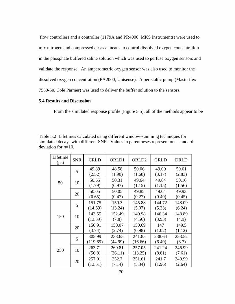
70
flow controllers and a controller (1179A and PR4000, MKS Instruments) were used to
mix nitrogen and compressed air as a means to control dissolved oxygen concentration
in the phosphate buffered saline solution which was used to perfuse oxygen sensors and
validate the response. An amperometric oxygen sensor was also used to monitor the
dissolved oxygen concentration (PA2000, Unisense). A peristaltic pump (Masterflex
7550-50, Cole Parmer) was used to deliver the buffer solution to the sensors.
5.4 Results and Discussion
From the simulated response profile (Figure 5.5), all of the methods appear to be
Table 5.2 Lifetimes calculated using different window-summing techniques for
simulated decays with different SNR. Values in parentheses represent one standard
deviation for n=10.
Lifetime
(μs) SNR CRLD ORLD1 ORLD2 GRLD DRLD
50
5 49.89
(2.52)
48.58
(1.90)
50.06
(1.68)
49.00
(3.17)
50.61
(2.83)
10 50.65
(1.79)
50.31
(0.97)
49.64
(1.15)
49.84
(1.15)
50.16
(1.56)
20 50.05
(0.65)
50.05
(0.47)
49.85
(0.27)
49.04
(0.49)
49.93
(0.45)
150
5 151.75
(14.69)
150.3
(13.24)
145.88
(5.07)
144.72
(5.33)
148.09
(6.24)
10 143.55
(13.39)
152.49
(7.8)
149.98
(4.56)
146.34
(3.93)
148.89
(4.9)
20 150.91
(3.74)
150.07
(2.74)
150.69
(0.98)
147
(1.02)
149.5
(1.12)
250
5 305.99
(119.69)
238.65
(44.99)
241.85
(16.66)
238.64
(6.49)
253.52
(8.7)
10 263.71
(56.8)
260.81
(36.11)
257.05
(13.25)
241.24
(8.81)
246.99
(7.61)
20 257.01
(13.51)
252.7
(7.14)
251.61
(5.34)
241.7
(1.96)
249.99
(2.64)

71
very accurate at low oxygen concentrations; that is, when the windows are able to cover
most of the decay. However, at higher oxygen concentrations, DRLD and GRLD were
the only methods to keep a high accuracy, as indicated by the high R2 values (>0.99) for
both methods (Table 5.1). The decrease in accuracy at higher lifetimes is a result of the
large amount of neglected data, as suggested by Figure 5.3. The original window-sums
technique, CRLD, had the worst accuracy out of all of the methods and reinforces the
limitation of fixed window widths. This initial testing suggested that DRLD would be
able to perform well under dynamic testing conditions.
Figure 5.6 Example decays obtained from the custom lifetime measurement system for
each oxygen concentration tested.

72
The results from simulations that tested the effects of SNR can be found in Table
5.2. As expected, increasing the SNR leads to a decrease in the variability for each
window-sum lifetime calculation method. However, as suggested by the results in
Figure 5.5, this does not mean that the accuracy of the calculation increases. For
example, the GRLD calculations for the 250 μs decay were not within one standard
deviation of the actual lifetime for any SNR. The DRLD method, however, was always
within one standard deviation of the actual lifetime and showed variability that was the
same order of magnitude or less than the other methods. The variability for higher
lifetime values was generally less than the other window sum methods with equal
window width and more accurate than the GRLD method. This suggests that the DRLD
method is better suited to determine the lifetime response for a range of values.
Table 5.3 R2 values for NLLS exponential fittings of lifetime decays and calculated
SNR at each concentration. Percent difference from NLLS for the different window-
summing methods is also shown for each oxygen concentration.
[O2]
(μM) R
2 SNR
NLLS
Lifetime
(μs)
Percent Difference from NLLS
DRLD CRLD ORLD1 ORLD2 GRLD
0 0.97 43.2 277.07 0.680 -15.4 -13.5 -11.8 -10.0
27.3 0.89 22.6 117.28 2.50 -10.6 -8.61 -4.68 -2.43
52.1 0.78 15.7 91.48 0.295 -13.0 -9.30 -4.87 -0.420
76.4 0.56 8.95 62.24 8.21 -3.77 -1.44 5.65 5.42
101 0.51 6.45 58.45 1.49 -8.47 -2.35 2.13 2.34
125 0.33 5.24 46.84 2.13 -1.56 -1.73 2.89 -5.38

73
Using decays experimentally obtained using the custom lifetime measurement
system (Figure 5.6); the lifetimes were calculated for each method and plotted for
comparison (Table 5.3, Figure 5.7). It appears that the lifetimes calculated from the real-
time decay data follow the trends observed from to the simulated profiles. The NLLS
calculations did not have very high R2 values at higher oxygen concentrations due to
increased quenching of the dye’s luminescence intensity which lead to a lower SNR
(Table 5.3). From these fittings, was found to be 162 μs. When comparing the
window-summing techniques, DRLD showed a much higher accuracy than the other
methods and was not significantly different than NLLS lifetimes (α = 0.05). The other
Figure 5.7 Lifetime response profile of the different window-sum methods compared to
the lifetime calculated using traditional fittings. Error bars represent 95% confidence
interval with n=25.
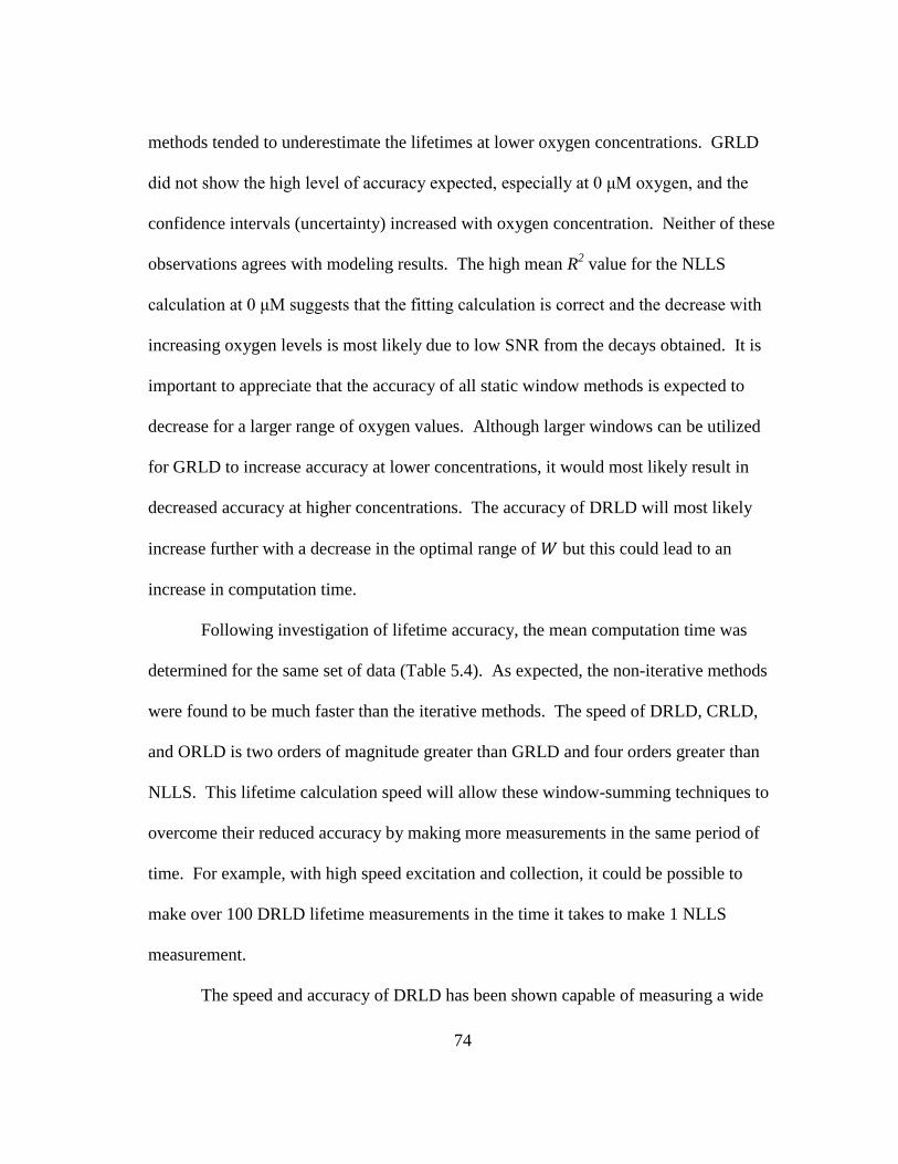
74
methods tended to underestimate the lifetimes at lower oxygen concentrations. GRLD
did not show the high level of accuracy expected, especially at 0 μM oxygen, and the
confidence intervals (uncertainty) increased with oxygen concentration. Neither of these
observations agrees with modeling results. The high mean R2 value for the NLLS
calculation at 0 μM suggests that the fitting calculation is correct and the decrease with
increasing oxygen levels is most likely due to low SNR from the decays obtained. It is
important to appreciate that the accuracy of all static window methods is expected to
decrease for a larger range of oxygen values. Although larger windows can be utilized
for GRLD to increase accuracy at lower concentrations, it would most likely result in
decreased accuracy at higher concentrations. The accuracy of DRLD will most likely
increase further with a decrease in the optimal range of but this could lead to an
increase in computation time.
Following investigation of lifetime accuracy, the mean computation time was
determined for the same set of data (Table 5.4). As expected, the non-iterative methods
were found to be much faster than the iterative methods. The speed of DRLD, CRLD,
and ORLD is two orders of magnitude greater than GRLD and four orders greater than
NLLS. This lifetime calculation speed will allow these window-summing techniques to
overcome their reduced accuracy by making more measurements in the same period of
time. For example, with high speed excitation and collection, it could be possible to
make over 100 DRLD lifetime measurements in the time it takes to make 1 NLLS
measurement.
The speed and accuracy of DRLD has been shown capable of measuring a wide
75
range of lifetimes for a common oxygen sensing system. These calculations displayed a
high degree of accuracy and precision over a variety of oxygen concentrations. The
DRLD technique can be easily implemented with a wide variety of current and future
sensor technologies for analyte measurement.
5.5 Conclusions
After investigation, DRLD was found to be more accurate than other window-
summing lifetime calculation techniques with fixed window sizes when a wide range of
lifetime values were considered. For the static window-summing methods, it is
necessary to know beforehand the average expected lifetime to make accurate lifetime
predictions. In contrast, DRLD is always accurate because it adjusts the window size
and, despite this iterative approach, it is still more than one thousand times faster than
traditional NLLS calculations. It is noteworthy that this algorithm may also be used with
charge-coupled device (CCD) detectors with the window change not occurring until the
Table 5.4 Real-time computation data for each window-based lifetime measurement
technique. Values in parentheses represent standard deviation with n = 25.
Method
Mean
Computation
Time (ms)
NLLS 307 (65.6)
DRLD 0.197 (0.043)
CRLD 0.143 (0.045)
ORLD1 0.137 (0.010)
ORLD2 0.149 (0.055)
GRLD 13.6 (0.200)

76
next lifetime measurement. This dynamic windowing algorithm can be implemented
additional degrees of freedom, such as with overlapping windows in order to increase
the optimal range of or with a three-window-sum calculation which does not
require the background signal to be measured beforehand.28, 181
With the aid of current
microprocessor technology, it is anticipated that this method can be utilized within
numerous sensing applications to enable accurate dynamic lifetime predictions using
low-cost mobile devices.
77
6. DUAL DYNAMIC RAPID LIFETIME DETERMINATION
Luminescent sensing has become an area of interest in a variety of industries due
to the greater sensitivity and measurement flexibility offered over other measurement
methods including electrochemical. 4, 156
Oftentimes, multiplexed sensors or multi-
sensors capable of measuring several analytes are needed for diagnostic and/or
compensation purposes.26
For example, temperature compensation is often needed of
luminescent oxygen sensors.162, 190, 192, 199-206
A key issue of multiplexing, however, is
the separation of the individual sensor responses.26
In the past, sensors capable of
monitoring multiple analytes or multi-sensors were measured using intensity
measurements; however, spectral cross-talk or overlap must be avoided.26
Finding
luminophores with adequate sensitivity, selectivity, and stability while still maintaining
this spectral distinction may be difficult.207
Even if appropriate luminophores are found,
additional optical hardware will be required in order to separate the emission signals
and/or excite the respective luminophores. In addition, intensity measurements are
susceptible to errors due to photobleaching of the luminophore, optoelectronic drift, or
variations in luminophore concentrations from sensor-to-sensor (see Chapter 4 for more
details).24, 114
Luminescence lifetime measurements are able to overcome these problems
by determining the rate of luminescence decay using temporally-resolved measurements
in the time- or frequency-domain (TD and FD, respectively). Advances in technology in
recent years have allowed these types of measurements to become more common. 24
Several methods have already been reported which temporally-resolve the
response of multiple sensors with distinct lifetimes. Although multi-sensor lifetime

78
measurements can be made by optically filtering the signal from spectrally-distinct
luminophores, this again requires spectrally-distinct luminophores.162
As an alternative,
many TD and FD methods have been developed which utilize luminophores with
distinct decay times.156, 162, 190, 192
These and other approaches that utilize temporal-
based measurements have been recently reviewed elsewhere; only dual lifetime
calculation techniques will be discussed herein.165
Multi-lifetime calculations in the frequency-domain (FD) require phase or
modulation measurements at multiple frequencies. Non-linear least-squares analysis
(NLLS) is used to fit the frequency dependent response data and determine the
lifetimes.149
Fittings, however, are computationally intense and dependent on the initial
guesses which can be an issue for highly sensitive luminophores where the lifetime and
intensity are expected to have a wide dynamic range.25
The increased computational
intensity can affect the speed of calculation and thus the real-time measurement
capabilities. In addition, FD calculations can suffer from errors in vivo due to scattered
excitation light and tissue autofluorescence. TD measurements, however, can easily
remove these short-lived signals (typically ≤10 ns) by delaying the lifetime calculation
of the longer-lived luminophores until after these events have decayed to zero.
In the TD, the decay data obtained are typically fit using NLLS to a multi-
exponential curve:
( )
⁄
⁄ 6.1
where and refer to the initial intensity and lifetime of the response of the
luminophore with a shorter lifetime, . Similarly, and describe the response of

79
the luminophore with the longer lifetime, . An example of a multi-exponential decay
can be seen in Figure 6.1.
As with mono-exponential lifetime calculations, several methods have been
developed to simplify multi-exponential lifetime measurements. This can be done by
separating the response of from the combined response (Figure 4.3). This allows
mono-exponential calculations to be used for each response assuming the contribution
from is constant during the decay of (see Figure 4.3). This technique has been
demonstrated with a windowed calculation technique (Dual Lifetime Determination) and
NLLS.156, 162, 190, 192
However, this may not be practical in cases where the lifetimes are
Figure 6.1 Diagram showing the combined response of a shorter-lived luminophore, , and a longer-lived luminophore, .

80
not different by three orders of magnitude which will result in being dependent on the
response of . A similar approach utilizes four equi-width windows, either contiguous
or overlapping, to calculate both lifetimes without separation of the signal (Figure
4.4).181
However, the accuracy of this method has been shown to be highly dependent
on signal level181
.191
The requirement of equi-width windows for both lifetime
measurements also means lifetimes must be similar in value ( ≈ 3 to 4) to ensure
that the window width is optimal and accurate lifetimes can be calculated.
Due to the limitations of these approaches, a new approach for dual lifetime
calculations was investigated. This method combines the Dynamic Rapid Lifetime
Determination (DRLD) discussed above and a window sum correction which will allow
accurate lifetime calculations of both dyes.
6.1 Theory
As an alternative to least-squares analysis, there have been several methods
developed which utilize window-sums to determine the lifetime responses.27-29, 171, 179-181,
183, 185, 188-189, 208 Window-sums are calculated by performing integration or adding the
data found in each windowed segment. Of the various methods reported, DRLD is of
particular interest for dual lifetime calculations because of its speed and simplicity (see
Chapter 5). This method calculates lifetimes using the traditional Rapid Lifetime
Determination (RLD) equation:
( ) 6.2

81
where is the lifetime, is the window width, and is the ratio of the window
sums from the respective windows.27-28
In addition, an algorithm is used to dynamically
select the appropriate window width. Without such a selection algorithm, the window
widths and start times remain constant during an experiment, leading to sub-optimal
sampling parameters and inaccuracies in many cases.27, 181, 188-189
For example, windows
that are too large will lead to sampling data that contains very little signal while
windows that are too small will be more greatly affected by the signal noise. However,
by optimizing the window width, the accuracy of lifetime calculation can be improved
Figure 6.2 Depiction of a dual-exponential decay and the window sums utilized to
calculate the lifetime response using DDRLD. The black dashed line represents the
combined response, while the blue and red dashed lines represent response of and , respectively. Example window sums are shown in the shaded regions.
82
over a wider dynamic range which is necessary for applications where the lifetime is
expected to vary (e.g. oxygen sensitive luminophores). In addition, this method retains
the speed of other approaches that utilize window sums when compared to the speed of
traditional NLLS calculations.153
To calculate the lifetimes of two luminophores, DRLD is utilized for each dye
where the windows for the calculation of were delayed until had decayed to zero
(Figure 6.2). In order to determine , the initial intensity of is calculated using:
(
⁄ )
⁄
6.3
where is the lifetime calculated using Equation 6.2, is the sampling frequency used
during measurement, is the time delay incorporated before sampling, and is the
respective window sum for each window. The time delay was incorporated to remove
unwanted scattering and instrument response. After is determined, the response of
can be subtracted from the measured (combined) signal; the resulting decay will be
representative of and is used to calculate with DRLD. Adjustment of the window
delay of the second set of windows to 5 times will allow improved accuracy of the
and subsequently improved accuracy of . This delay was chosen because the signal
from will be less than 1% of the original signal level and thus assumed to be
negligible during calculation of .

83
Dual lifetime calculations are done recursively until the window delay is no
longer changing. The initial window delay time for the second set of windows for both
calculation algorithms is initially set to a value greater than ten times the maximum
expected lifetime of (in this case 1000 μs) in order to ensure that there is not any
contribution from in the initial calculation. In addition, the maximum number of
Figure 6.3 Diagram showing a simplified version of the DDRLD algorithm.
84
iterations set for each algorithm is 10 in order to prevent infinite loops in the software
where lifetimes bounce back and forth between two values. However, in most cases less
iteration are needed. A simplified algorithm for this approach, which will be referred to
as dual DRLD (DDRLD), can be found in Figure 6.3. An example of the MATLAB
code used for DDRLD calculation can also be found in Appendix C. It should be noted
that for the algorithm to work properly, the decay of must behave mono-
exponentially.
6.2 Materials and Methods
In order to evaluate the potential of this method to accurately calculate the
lifetime response of two luminophores simultaneously, an oxygen and temperature
sensing system was employed. These analytes were chosen because of their biological
significance. In addition, temperature compensation of oxygen sensitive luminophores
is often necessary.162, 190, 192, 199-206, 209
Platinum porphyrins are attractive for oxygen
sensing due to their high sensitivity, large Stokes’ shift, good photostability, long
lifetimes, and emission in the red to NIR wavelengths.210-218
Platinum(II)
octaethylporphyrin (PtOEP) has excitation peaks close to 400, 500, and 550 nm and
emission peaks near 650 nm.203, 219
The lifetime of this dye in the absence of oxygen is
also expected to be approximately 100 μs.219
An inorganic phosphor, manganese(IV)-
doped magnesium fluorogermanate (MFG), was used for temperature sensing because it
does not display oxygen sensitivity.220
The phosphor has an excitation peak near 400
nm, emits at 665 nm, and has a lifetime greater than 3 ms.220-221
These luminophores
were chosen because they both showed a large Stoke’s shift and can be excited with a
85
single LED at 400 nm. The large difference in lifetime will also reduce the chance of
inaccuracies occurring as was seen with similar approaches.181
The overlap in emission
spectra is not a concern because the response from each luminophore is resolved
temporally.
Although DDRLD would ideally be performed with oxygen and glucose sensors
in order to demonstrate in vitro the oxygen compensation method discussed in Chapter
3. However, due to the degradation often associated with enzymatic sensors,
repeatability may be an issue. The dual sensing system described above will serve as an
analogue of the desired oxygen and glucose sensing system because of its simplicity and
higher expected repeatability (due to the absence of enzymatic components). Further
considerations for employing DDRLD for measuring the response of glucose and
oxygen sensors simultaneously will be discussed in Chapter 7.
6.2.1 Modeling of Dual Exponential Decays
Due to the large difference in lifetimes expected from PtOEP and MFG, dual
exponential decays were also modeled using MATLAB to test the ability of DDRLD to
distinguish decays from one another for a range of lifetimes and pre-exponential factors.
This was done by setting and to 1 and 10 μs, respectively, while and were
varied from 0.01 to 100 and 15 to 100 μs, respectively. This allows for the accuracy to
be estimated as a function of the ratios and . For each possible combination
of decay parameters, ten decays were modeled using a sampling frequency of 2 MHz
and a signal-to-noise ratio (SNR) of 10 in order to simulate real decays obtained.
Lifetimes were then calculated using DDRLD with the first window delay set to 1 μs and

86
the second window delay set to five times (50 μs) which is where it ideally remain
due to the algorithm restrictions (Figure 6.3). Initial widths of each window pair were
set to 10 μs. From these data, the relative standard deviation (RSD) of each lifetime was
determined for each set of decay parameters by dividing the standard deviation by the
average lifetime calculated. Absolute percent difference was also investigated by
comparing the mean lifetime at each and value to the modeled value. These
parameters characterized the precision and accuracy of lifetime calculations, respectively
and allowed analysis of the results to determine the optimal relative pre-exponential
factors and lifetimes similar to previous reports.27-28, 181, 188-189
6.2.2 Sensor Formulation
PtOEP was purchased from Frontier Scientific and MFG was obtained from
Global Tungsten & Powders Corp. (GTP Type 236). Similar to previously reported
oxygen sensors, polystyrene (PS, Sigma, Mw=280,000) was utilized to slow oxygen
diffusion through the matrix leading to higher lifetimes of the oxygen-quenchable
dye.213, 216
Toluene (Macron Chemicals) was used as a solvent for PtOEP and PS. A
Sylgard 184 silicone elastomer kit (Dow Corning) was used to make
polydimethylsiloxane (PDMS) films for support of each phosphor during testing.
Temperature sensing gels were made by mixing 3 mg of MFG in 2 mL of PDMS
precursor and 200 μL of PDMS initiator. The solution was sonicated and then placed
under vacuum until all bubbles were removed and then poured on a glass wafer. The
wafer was then placed on a hot plate at 100°C to facilitate PDMS curing. The resulting
film was approximately 4 cm in diameter. Although films were thoroughly mixed

87
before curing, aggregation of the phosphor was visible after curing and resulted in
inhomogeneities in the film. The oxygen sensing film was made using a similar
procedure. Fifteen μL of PtOEP solution (1 mg/mL of toluene) and 700 μL of
polystyrene solution (250 mg/mL of toluene) were mixed with 1 mL of PDMS precursor
and 100 μL of PDMS initiator. After vacuuming and heat curing, the resulting film was
again approximately 4 cm in diameter. For individual film testing, a 2.5 mm biopsy
punch was used to remove samples from each film for testing. Dual sensor measurement
was performed by cutting the previously tested films in half and placing MFG and
PtOEP films side-by-side (Figure 6.4).
6.2.3 Instrumentation and Measurement
The luminescent response of each of the sensors tested was measured using a
custom TD measurement system.153
Excitation of the dye was performed using an LED
with a peak wavelength of 405 nm (LED 405E, Thorlabs). Square wave excitation with
a frequency of 10 Hz and a duty cycle of 0.2 was utilized. Luminescence was detected
Figure 6.4 This picture shows examples of films tested. The sensor on the far left is an
oxygen sensing film containing PtOEP and the sensor on the right is a temperature
sensing film containing MFG. The sensor in the middle consists of halves of each film
placed side-by-side.
88
using a photo-multiplier tube module from Hamamatsu (H10721-20) after the light was
passed through a longpass filter (3rd Millenium 620 nm, Omega Optical) using spherical
lenses (LA-1951B). Decays were recorded for 15 ms with a sampling frequency of 2
MHz after the LED was turned off. For MFG and dual film experiments, the PMT
control voltage was set to 0.85 V. Due to the wide range of intensities observed, a lower
control voltage, 0.75 V, was used with PtOEP films to prevent saturation of the detector.
During measurement, one hundred raw decays were summed to improve SNR and the
resulting decay was used to calculate the lifetime. Further details of this measurement
system can be found in Appendix A.
The gas-phase response of the sensors was measured using a custom reaction
chamber.152-153
The sensing films were immobilized in the reaction chamber by placing
them on a glass slide which was then placed inside of an incubator (Torrey Pines
Scientific, Echotherm IN35) used to control the temperature (25 to 65°C). Gas of
various oxygen concentrations (0 to 21%) were exposed to the sensors by controlling
compressed air and nitrogen flow rates using two mass flow controllers (MKS
Instruments, 1179A) and a digital power supply (MKS Instruments, PR4000). The total
flow rate was held constant at 2000 standard cubic centimeters per minute while the
contribution from each gas was varied. All parts of the test-bench were automated and
controlled using custom LabVIEW software (National Instruments). Further details of
this test system can be found in Appendix B.
For this work, lifetime calculations for calibration purposes (single and dual
films) were performed after data collection with MATLAB (MathWorks, Inc.). DRLD
89
was used to calculate the mono-exponential lifetimes for individual films while lifetimes
of dual films were calculated using DDRLD. NLLS analysis with a mono-exponential
fit was used to calculate lifetimes for individual films for comparison purposes. Real-
time calculations utilizing DDRLD were performed with LabVIEW during a dynamic
response experiment. In order to calculate lifetimes, windows used for MFG and PtOEP
were set to an initial width of 200 and 5 μs, respectively. All single film experiments
had an initial window delay of 1 μs while dual film experiments had 1 μs delay for
PtOEP and an initial delay of 1000 μs for MFG as discussed above.
6.2.4 Film Testing and Analysis
Initially, individual PtOEP and MFG films were each tested in triplicate. For
each test, ten lifetimes were averaged for each environmental condition (i.e. oxygen
concentration and temperature) tested. The response of the three individual films was
then averaged to determine the expected response from dual film measurements. For
MFG films, the lifetime response of MFG films was recorded at five different
temperatures (25 to 65°C in 10° increments) using an oxygen concentration of 21%.
Linear regression was then used to fit the averaged film responses and obtain a
calibration for the temperature sensitive MFG response.
To keep testing time to a minimum, calibration of the PtOEP films was
performed at only three temperatures (25, 45, and 65°C) but for a range of oxygen
concentrations at each temperature. These concentrations (0, 2.625, 5.25, 10.5, and 21%
oxygen) were skewed towards lower oxygen levels where sensitivity of the porphyrin is

90
higher. The response at each temperature was fit with NLLS using a two-site Stern-
Volmer equation:
(
[ ]
[ ])
6.4
where , is the lifetime in the absence of the quencher (in this case oxygen ), is the
lifetime, is the fractional contribution from each site, and is the respective Stern-
Volmer constant.19, 211, 214, 222
After initial fittings, the fractional contribution was
averaged and used to re-fit the data to allow more accurate temperature-dependent trends
to be determined. It is assumed that this value remains constant despite temperature
changes. The temperature-dependent trends of the parameters ( , , and ) in
Equation 6.4 were then determined using linear regression.
As previously mentioned, dual film responses were measured using the same
measurement system with a side-by-side approach where halves of the previously tested
films were utilized. Testing of the dual film response was performed similar to testing
of PtOEP films. The validity of DDRLD was investigated by comparing the lifetimes
obtained from the dual films with the response of the individual films.
A dynamic experiment was also performed to demonstrate the ability of DDRLD
to measure the response of a dual luminescent system. This was done by exposing the
dual films to random, un-calibrated temperatures and oxygen concentrations. When
temperature was changed, the experimental setup was held there (i.e. temperature and
oxygen was not changed) for 2 hours to ensure the temperature throughout the reaction
chamber reached equilibrium. Changes in oxygen concentration were only held for 15
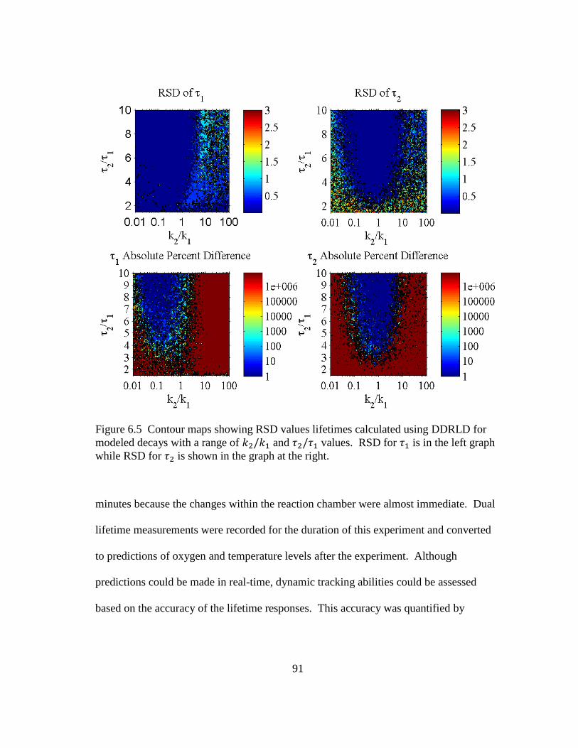
91
minutes because the changes within the reaction chamber were almost immediate. Dual
lifetime measurements were recorded for the duration of this experiment and converted
to predictions of oxygen and temperature levels after the experiment. Although
predictions could be made in real-time, dynamic tracking abilities could be assessed
based on the accuracy of the lifetime responses. This accuracy was quantified by
Figure 6.5 Contour maps showing RSD values lifetimes calculated using DDRLD for
modeled decays with a range of and values. RSD for is in the left graph
while RSD for is shown in the graph at the right.

92
calculating the percent difference for n = 10 predictions at each oxygen and temperature
combination tested.
6.3 Results and Discussion
6.3.1 Results of Modeled Dual-Exponential Lifetime Calculations
RSD and absolute percent difference values obtained after modeling DDRLD
calculations for a range of values for and can be seen in Figure 6.5. These
graphs showed good agreement about the relative parameters needed for optimal dual
lifetime calculations. Accuracy appears to be highest when is between 0.1 and 1
where the blue regions of each absolute percent difference contour map overlap.
Lifetime calculations are also more accurate when is greater than 3. RSD contour
maps display similar trends but with a slightly larger optimal area (values represented by
blue).
When the relative decay parameters fall outside of this region, DDRLD suffers
from a drastic reduction in accuracy for modeled decays with an SNR of 10. A higher
SNR will likely lead to wider optimal regions, but these results clearly indicate the
limitations of this method under normal working conditions. These results should be
utilized to select luminophores with the appropriate lifetimes. Intensity is less of a
concern when selecting luminophores because it is not an inherent property of the
luminophore and can be adjusted by changing the concentration.
6.3.2 Calibration of Individual Film Responses
The response of individual MFG films can be seen in Figure 6.6. Although the
response from film-to-film was statistically different, each response follows the same
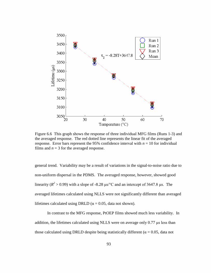
93
general trend. Variability may be a result of variations in the signal-to-noise ratio due to
non-uniform dispersal in the PDMS. The averaged response, however, showed good
linearity (R2 > 0.99) with a slope of -8.28 μs/°C and an intercept of 3647.8 μs. The
averaged lifetimes calculated using NLLS were not significantly different than averaged
lifetimes calculated using DRLD (α = 0.05, data not shown).
In contrast to the MFG response, PtOEP films showed much less variability. In
addition, the lifetimes calculated using NLLS were on average only 0.77 μs less than
those calculated using DRLD despite being statistically different (α = 0.05, data not
Figure 6.6 This graph shows the response of three individual MFG films (Runs 1-3) and
the averaged response. The red dotted line represents the linear fit of the averaged
response. Error bars represent the 95% confidence interval with n = 10 for individual
films and n = 3 for the averaged response.

94
shown). The difference is most likely due to the multi-exponential nature of the decays
for PtOEP which is often dependent on the immobilization matrix.222-224
Similar to
reports of other oxygen sensitive luminophores, the oxygen sensitivity was higher at
lower oxygen concentrations and increases in temperature lead to decreases in the
lifetime response.162, 190, 200
Due to the non-linear nature (see Equation 6.4) of the
oxygen response as well as the temperature dependency, calibration of the PtOEP films
required more thorough analysis in order to predict oxygen concentrations accurately
(Figure 6.7).
Figure 6.7 Response of individual PtOEP films to oxygen and temperature. Error bars
represent the 95% confidence interval with n = 10 for individual films (Runs 1-3) and n
= 3 for averaged data.

95
First, the Stern-Volmer plot for the response at each temperature was determined
using the appropriate values for (Figure 6.8). After initial fitting using Equation 6.4,
the mean fractional intensity, , was found to be 0.278. This value was used to re-fit the
Stern-Volmer responses and the resulting trends of and as a function of
temperature ( ) were found. These values along with the temperature dependent values
for can be found in Figure 6.9. The linear fits used for calibration of , , and
all had an R2 value greater than 0.99. This indicates that these trends can be used to
estimate the oxygen concentration for all temperatures within or near the tested range as
long as the ambient temperature is accurately predicted. When these values were
Figure 6.8 Stern-Volmer response of the PtOEP films. The red line represents the fit
obtained using Equation 6.4 which was used for calibration.

96
plugged into Equation 6.4 and compared to the original data, R2 remained greater than
0.99.
6.3.3 Dual Film Responses
Following calibration of the individual film responses, the lifetimes of dual films
calculated using DDRLD were compared to the response of individual films where the
lifetimes were calculated using DRLD. As can be seen in Figure 6.10, the MFG
response calculated using DDRLD for dual film measurements was not significantly
different than the average DRLD response for any condition tested. Although it appears
Figure 6.9 Temperature ( ) dependent trends for , , and can be seen in the
top left, bottom left, and bottom right images, respectively. The red lines show the
linear fit obtained for each set of data. The top right image shows the initial fractional
intensities obtained where the red line represents mean value that was used to obtain
and .

97
that the lifetime increases slightly with increasing oxygen concentration, this is not
statistically significant and is actually due to a decrease in the noise as luminescence
decays (data not shown). Increasing delay in the windows used for calculation, as is
done for DDRLD calculation, results in a slight shift in the calculated lifetime.
Improvements in SNR throughout the decay are expected to reduce this issue.
As expected, PtOEP lifetimes calculated using DDRLD for dual film
measurements followed the same trends as individual film data (Figure 6.11). However,
the lifetimes calculated for dual films were statistically different than results calculated
for individual films. Despite this, the average percent difference for the dual film
Figure 6.10 Comparison of the MFG lifetime response for individual and dual film
experiments where lifetimes were calculated using DRLD and DDRLD, respectively.
Error bars represent the 95% confidence interval for n = 3 films.
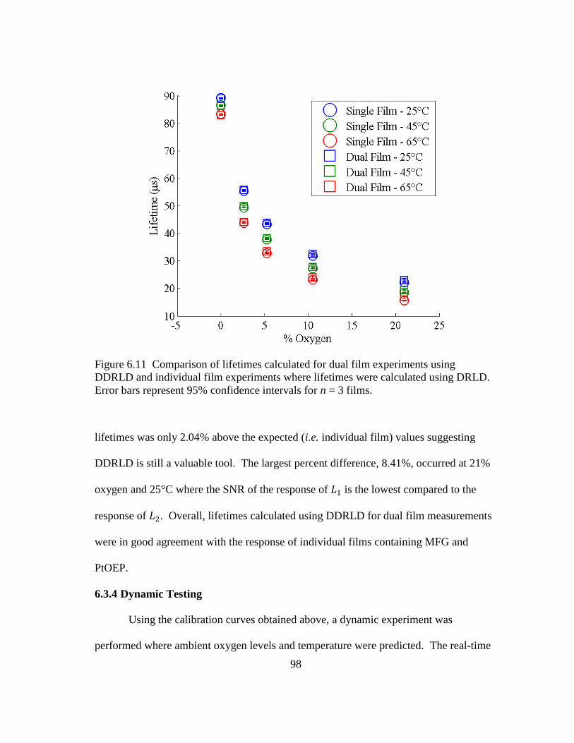
98
lifetimes was only 2.04% above the expected (i.e. individual film) values suggesting
DDRLD is still a valuable tool. The largest percent difference, 8.41%, occurred at 21%
oxygen and 25°C where the SNR of the response of is the lowest compared to the
response of . Overall, lifetimes calculated using DDRLD for dual film measurements
were in good agreement with the response of individual films containing MFG and
PtOEP.
6.3.4 Dynamic Testing
Using the calibration curves obtained above, a dynamic experiment was
performed where ambient oxygen levels and temperature were predicted. The real-time
Figure 6.11 Comparison of lifetimes calculated for dual film experiments using
DDRLD and individual film experiments where lifetimes were calculated using DRLD.
Error bars represent 95% confidence intervals for n = 3 films.

99
temperature prediction from the MFG response compared to the temperature
programmed into the incubator can be seen in Figure 6.12, and as expected, the MFG
response is able to track the ambient changes in temperature. Calculating the percent
difference for n = 10 predictions at each concentration and temperature, the average
percent difference for all concentrations and temperatures was found to be 0.72%
suggesting an accurate prediction of temperature. It is important to note that the slow
response time observed for MFG is due to the long equilibration time of the incubator
and reaction chamber and not the sensor film.
Oxygen predictions performed with compensation showed a similar ability to
Figure 6.12 Results of a dynamic test showing programmed and predicted temperatures.
DDRLD was utilized to monitor the lifetime responses of the two films simultaneously.
Temperature predictions were determined from a linear calibration curve.

100
track oxygen levels as temperature predictions; however, predictions tended to be lower
than the actual levels (Figure 6.13). At 15.75% oxygen, the relative error for
compensated predictions was found to be 8.77% but at the lowest levels tested (2.1%
oxygen), the response was off by only 0.63% (Table 6.1). This improved accuracy at
lower oxygen levels is due to an increase in intensity from the PtOEP resulting in a
higher SNR. The reduced accuracy in oxygen prediction at higher oxygen
concentrations is due to the exponential shape of the oxygen response curve and the
difference in PtOEP lifetimes calculated using DRLD and DDRLD (discussed above).
Figure 6.13 This graph depicts the programmed and predicted oxygen concentrations
from a dynamic test. DDRLD was utilized to monitor the lifetime responses of the two
films simultaneously. A temperature compensating PtOEP calibration curve was used to
predict oxygen levels.

101
For example, the expected response of at 25°C and 21% oxygen is 22.3 μs, however,
if was measured to be 1 μs lower than the expected, the predicted oxygen
concentration would be 22.8%. Similarly, if the expected response of at 25°C and 0%
oxygen (89.3 μs) was low by 1 μs, the predicted oxygen concentration would be 0.04%.
Table 6.1 Percent differences calculated for n = 10 predictions during the dynamic
testing of dual film responses. Calibration type refers to calibrations made using either
single or dual film responses. Uncompensated results utilized the calibration curve at
40°C while compensated results utilize a variable calibration curve as discussed in the
text.
Oxygen (%) Calibration
Type Compens.
Temp.
(°C)
30 40 50
2.1
Single N 17.3 0.468 -17.8
Single Y -2.60 0.919 -0.200
Dual Y -4.35 -0.560 -1.59
4.2
Single N 18.1 4.59 -12.8
Single Y 0.82 3.42 3.72
Dual Y -1.17 1.46 1.65
6.3
Single N 20.2 6.18 -10.6
Single Y 3.93 5.66 5.14
Dual Y 1.61 3.10 2.14
8.4
Single N 20.7 6.70 -9.60
Single Y 5.46 7.07 5.90
Dual Y 2.64 3.75 1.84
15.75
Single N 21.3 9.00 -3.64
Single Y 7.09 9.07 10.14
Dual Y 2.16 3.04 3.04

102
These differences in predicted and actual oxygen levels indicate the greater effect
inaccurate lifetime calculations have at higher oxygen concentrations.
To improve the accuracy of lifetime predictions, calibration curves of the PtOEP
response using DDRLD data from Figure 6.11 were determined (data not shown). These
calibration curves were then utilized to make oxygen predictions for the same
dynamically obtained lifetimes utilized to obtain the predictions in Figure 6.13. As can
be seen in Figure 6.14 and Table 6.1, these results show a higher accuracy at higher
oxygen levels than predictions made using calibrations obtained from individual film
responses. Again, this is due to the difference in the lifetime response calculated for
Figure 6.14 Real-time dynamic oxygen predictions made using calibration curves
obtained from a dual film PtOEP response. The same lifetimes obtained from the
previously described dynamic experiment were utilized.

103
individual and dual film measurements using DRLD and DDRLD, respectively.
Oxygen predictions made with temperature compensation were also compared to
predictions made without compensation (assuming calibration was performed at 40°C).
As expected for predictions made when the programmed temperature was 40°C, the
compensated and uncompensated predictions have similar accuracy (Table 6.1).
However, when the actual temperature is not 40°C, uncompensated oxygen predictions
are much less accurate. This demonstrates the need for temperature compensation of a
luminescent oxygen sensor response when a range of ambient temperatures are expected.
Despite the inaccuracies of oxygen prediction, which could be reduced by
improving SNR, the usefulness of this approach is evident based on the predictions for
un-calibrated temperatures and oxygen concentrations. It is also interesting to note that
the oxygen predictions do not appear to be temperature dependent because the responses
at the same oxygen concentration but different temperatures appear to be the same.
6.4 Conclusions
A dual dynamic rapid lifetime determination (DDRLD) algorithm was
investigated that is able to calculate the lifetime response of two temporally-distinct
luminophores simultaneously. Using modeled decays, this dual lifetime calculation
approach was found to be limited multi-exponential decays where is greater than 3
and is between 0.1 and 1. This approach was demonstrated in vitro by performing
temperature compensation of an oxygen-sensitive porphyrin after calibrating an oxygen
sensing film at three different temperatures and determining the linear temperature
dependency of the calibration fit parameters. Lifetimes calculated for dual films using
104
DDRLD were compared to lifetimes calculated for individual films using DRLD. The
response of the temperature sensing films was not found to be statistically different.
Lifetimes of oxygen sensing films did display some difference but is considered to be
quite low on average (2%). Temperature compensation was then applied with DDRLD
to demonstrate real-time, dynamic predictions of oxygen and temperature.
Individually, each of the techniques demonstrated (a compensation algorithm
and a method for measuring two lifetimes simultaneously) can be applied to a variety of
sensing applications. The compensation method demonstrated will allow improved
accuracy in oxygen measurements. The simplicity of the approach will also lend its
usefulness to other applications where compensation is needed to improve the accuracy
of measurements of the desired analyte (such as oxygen compensation of enzymatic
glucose sensors). DDRLD can also be utilized with a variety of biomedical,
environmental, and food industry applications due to its ability to perform real-time
measurements without sacrificing accuracy.
105
7. CONCLUSIONS AND FUTURE WORK
Different computational and algorithmic techniques to improve the accuracy and
thus viability of luminescent, enzymatic sensors were proposed and demonstrated within
this work. These techniques will assist in the progression of these sensors toward in vivo
use by people with diabetes.
Due to the co-consumption of glucose and oxygen during the reaction of glucose
oxidase (GOx), an enzyme commonly used by glucose sensors, the dependence of the
response on ambient oxygen concentration was investigated in silico using COMSOL
Multiphysics. After confirmation of inaccurate glucose predictions due to variations in
the ambient oxygen concentration, a novel compensation technique was developed and
demonstrated. This approach utilized a variable calibration curve where the fit
parameters were determined as a function of oxygen levels which will be measured
separately. Using randomized oxygen and glucose levels based on expected in vivo
values, glucose predictions using the proposed compensation technique and un-
compensated predictions were compared. Even when measurement error was
considered, compensated predictions were located within the clinically acceptable
regions (A and B) of the standard Clarke error grid more than 95% of the time while un-
compensated predictions were within this region less than 50% of the time.
The compensation algorithm demonstrated utilizes a variable calibration curve
which is dependent on the interfering species. Due to its nature, this mechanism is
broadly applicable to a variety of enzymatic and other kinds of sensors where the
response follows predictable trends for both analytes. However, extensive calibration
106
will need to be performed for both analytes in order to understand these trends. In
addition, this approach may only be applied in instances where the confounding analyte
can be measured separately from the analyte of interest. Nevertheless, this approach will
lead to improved accuracy of a variety of analytes in instances where confounding
analytes are present.
This large improvement in accuracy using oxygen compensation led to the
investigation of a novel technique for monitoring two sensors simultaneously. Due to
the advantages of time-domain luminescence lifetime measurements over intensity and
frequency-domain lifetime measurements in vivo, this approach is ideal for measuring
the response of implantable luminescent sensors. The development of this approach was
first limited to the measurement of the response of a single sensor.
Building on the principles of Rapid Lifetime Determination, the Dynamic Rapid
Lifetime Determination (DRLD) method utilizes integration of two temporal windows in
order to quickly calculate the lifetime response. However, due to the inaccuracies that
result when static window widths are used for a wide range of lifetime responses, a
dynamic windowing approach was implemented. This resulted in improved accuracy of
lifetime calculations over a wider dynamic range as demonstrated by monitoring the
response of a luminescent oxygen sensor. In addition, DRLD displayed a calculation
time that was six orders of magnitude less than traditional non-linear least-squares
calculations of lifetime.
Due to the need for measurement of ambient oxygen concentration while
performing compensation of an enzymatic glucose sensor, DRLD was extended to

107
measurement of two lifetimes (and thus two sensors) simultaneously. The Dual DRLD
(DDRLD) approach requires luminophores with temporally-distinct lifetimes (at least
three times different) in order to separate the response of each sensor. Two pairs of
windows are required in order to calculate the lifetime of each luminophore. Initially,
the lifetime and initial intensity of the longer-lived luminophore is calculated by
delaying the second pair of windows until after the response of the shorter-lived dye has
decayed to zero. The response of this luminophore can then be removed from the total
signal allowing the lifetime of the shorter-lived luminophore to be calculated.
DDRLD was demonstrated using temperature and oxygen sensing films. These
analytes were chosen as a model system due to the temperature dependency of oxygen-
quenchable porphyrins. Similar to a glucose and oxygen sensing system, a variable
oxygen calibration curve that is dependent on the ambient temperature was utilized. An
inorganic phosphor was chosen as the temperature sensitive luminophore due its long
lifetimes (~3.5 ms) and insensitivity towards oxygen. Responses measured for films
containing a single luminophore showed good agreement with the responses measured
during measurement of both films simultaneously. In the case of the inorganic
phosphor, the single and dual film measurements were not significantly different.
Although oxygen sensitive films did display a statistical difference (α = 0.05) in the
response measurement for single and dual films, the average percent difference was only
2.04%. Using the results obtained, dynamic tracking of un-calibrated temperature and
oxygen values was demonstrated. As expected, compensated oxygen predictions

108
displayed more accuracy over a range of temperatures than un-compensated predictions
made using a static calibration curve.
The development of DDRLD provides a unique tool for the determination of
multiple luminescence lifetimes which can be employed with a variety of luminescent,
multi-analyte sensors which are often needed for compensation or diagnostic purposes.
The variety of implementations may be limited to the ability to find luminophores or
develop luminescent sensors (e.g. enzymatic sensors where the response is measured
indirectly) with enough temporal-resolution between the lifetimes (see Chapter 6).
However, it will be easier to implement sensors using DDRLD because actual lifetime
responses are measured which allows calibration of these sensors to be performed
individually unlike many ratiometric-based time-resolved measurements. In addition,
the speed of computation over non-linear least-squares calculations will allow
implementation of this algorithm with low-cost, portable electronics. Furthermore, the
development of DDRLD provides a mechanism whereby oxygen compensation of
enzymatic glucose sensors can be measured in vivo.
Employing DDRLD to perform oxygen compensation in the future will require
the use of two oxygen-sensitive dyes will not to be utilized; one for glucose sensing and
one for oxygen sensing. However, the lifetime of these luminophores must remain
sufficiently distinct as discussed above. This can be achieved by utilizing porphyrins
with different metal ions (i.e. platinum and palladium) bound to the center. Palladium
porphyrins have been shown to have a lifetime that is an order of magnitude longer in
the absence of oxygen than platinum porphyrins with the same structure.219
Assuming

109
the glucose concentration never reaches zero, the ambient oxygen concentration will
always be greater than oxygen levels inside glucose sensors which will allow oxygen
and glucose sensors to utilize a platinum and palladium porphyrin, respectively. The
glucose sensor must utilize the longer-lived palladium porphyrin because the
consumption of oxygen within the sensor will lead to increases in the lifetime. This will
help ensure that each luminophore response can be resolved at lower oxygen
concentration where the lifetimes have less temporal distinction (see below).
Figure 7.1 Measured lifetime responses of a palladium porphyrin and the estimated
lifetime response of a platinum porphyrin of the same structure and immobilized in the
same matrix (see text). The inset shows the response of the platinum porphyrin in
greater detail.

110
Modeling was again utilized to predict the simultaneous response of these
oxygen and glucose sensors. The relative response of a platinum porphyrin to a
palladium porphyrin with the same molecular structure and immobilized in the same
matrix was estimated by reviewing the literature. For both and , palladium
porphyrins were found to have values that were approximately seven times larger than
values for platinum porphyrins.224-226
Using this information, the response of a platinum
porphyrin immobilized in a pHEMA matrix was estimated using the data from Chapter 3
(Figure 7.1).
Figure 7.2 Values in circles represent the modeled response of an enzymatic glucose
sensor utilizing a palladium porphyrin to a range of glucose and oxygen values. Lines
are used to represent the response of an oxygen sensor utilizing a platinum porphyrin
because the response is independent of glucose concentration. Circles and lines with the
same color represent the response to a specific oxygen level shown in the legend.

111
Following estimation of a platinum porphyrin response, modeling was utilized to
determine the combined response for a dual oxygen and glucose sensing system. Similar
to the work performed in Chapter 3, a GOx concentration of 1.62e-10 M was utilized
with the diffusion coefficients of glucose and oxygen each set to 1e-11 m2/s. Using
these parameters, the lifetime responses were predicted for a range of glucose (0 to 400
mg/dL) and oxygen (20 to 140 μM) concentrations. The results can be found in Figure
7.2 where the line represents the expected oxygen response which is independent of
glucose concentration and the circle markers show the expected glucose sensor response.
As expected, the lifetime of the glucose sensor was always higher than the response of
the oxygen sensor. However, higher oxygen concentrations and lower glucose values
produced lifetimes that were not sufficiently distinct as determined in Chapter 6 (Table
7.1). The predicted results at 0 mg/dL are not a concern because in vivo glucose levels
are not expected to get this low. However, glucose values greater than 40 mg/dL this
remains an issue which will lead to less accurate glucose predictions when oxygen is
greater than 50 μM. This suggests that the current formulation will be viable for only
Table 7.1 Ratio of the glucose sensor lifetime response to the oxygen sensor lifetime for
the oxygen and glucose values modeled. Shaded areas represent values that are below
the required ratio needed to obtain accurate results ( > 3).
[glucose]
(mg/dL)
[O2] (μM)
20 50 80 110 140
0 2.95 1.97 1.65 1.49 1.39
40 4.82 3.25 2.46 2.04 1.80
100 5.08 3.89 3.18 2.71 2.37
200 5.17 4.16 3.59 3.19 2.88
400 5.21 4.31 3.84 3.51 3.26

112
low oxygen concentrations (< 50 μM). However, variability and baseline oxygen
concentrations at in vivo implantation sites are still not widely characterized, unlike
oxygen pressure (see Chapter 3). A better understanding of these values and additional
tailoring of the response of each sensor will lead to improve the temporal distinction
leading to glucose measurements with a higher degree of accuracy.
Future work will entail the in vitro validation of the proposed method for oxygen
compensation of enzymatic glucose sensors. After thorough characterization of oxygen-
dependence of the sensor through testing at a range of oxygen and glucose levels,
development of a dual sensing matrix or configuration for oxygen and glucose will be
investigated. I hypothesize that DDRLD can then be used in conjunction with the
oxygen compensation algorithm to accurately predict in vivo glucose levels. The
development of these techniques will lead to improved glucose monitoring and thus
reduced risk of health complications related to diabetes.

113
REFERENCES
1. American Diabetes Association. Diabetes Care 2004, 27. s91-s93.
2. Brauker, J. Diabetes Technol. Ther. 2009, 11. S-25-S-36.
3. McNichols, R. J.; Cote, G. L. J. Biomed. Opt. 2000, 5. 5-16.
4. Pickup, J. C., Hussain, F., Evans, N. D., Rolinski, O. J.; Birch, D. J. S. Biosens.
Bioelectron. 2005, 20. 2555-2565.
5. Pickup, J. C., Hussain, F., Evans, N. D.; Sachedina, N. Biosens. Bioelectron.
2005, 20. 1897-1902.
6. Khalil, O. S. Clin. Chem. 1999, 45. 165-177.
7. Oliver, N. S., Toumazou, C., Cass, A. E. G.; Johnston, D. G. Diabet. Med. 2009,
26. 197-210.
8. Steiner, M.-S., Duerkop, A.; Wolfbeis, O. S. Chem. Soc. Rev. 2011, 40. 4805-
4839.
9. Wilson, R.; Turner, A. P. F. Biosens. Bioelectron. 1992, 7. 165-185.
10. Brown, J. Q., Srivastava, R.; McShane, M. J. Biosens. Bioelectron. 2005, 21.
212-216.
11. Brown, J. Q., Srivastava, R., Zhu, H.; McShane, M. J. Diabetes Technol. Ther.
2006, 8. 288-295.
12. Brown, J. Q.; McShane, M. J. Biosens. Bioelectron. 2006, 21. 1760-1769.
13. McShane, M. J., Microcapsules as “Smart Tattoo” Glucose Sensors: Engineering
Systems with Enzymes and Glucose-Binding Sensing Elements. In Topics in
Fluorescence Spectroscopy: Glucose Sensing, ed. C. D. Geddes, J. R. Lakowicz.
Springer: New York, NY, 2006, vol. 11, pp 131-163.
14. Gough, D. A., Lucisano, J. Y.; Tse, P. H. S. Anal. Chem. 1985, 57. 2351-2357.
15. Leypoldt, J. K.; Gough, D. A. Anal. Chem. 1984, 56. 2896-2904.
16. Parker, J. W.; Schwartz, C. S. Biotechnol. Bioeng. 1987, 30. 724-735.
17. Stein, E. W., Grant, P. S., Zhu, H. G.; McShane, M. J. Anal. Chem. 2007, 79.
1339-1348.

114
18. Healey, B. G., Li, L.; Walt, D. R. Biosens. Bioelectron. 1997, 12. 521-529.
19. Li, L.; Walt, D. R. Anal. Chem. 1995, 67. 3746-3752.
20. Pasic, A., Koehler, H., Schaupp, L., Pieber, T. R.; Klimant, I. Anal. Bioanal.
Chem. 2006, 386. 1293-1302.
21. Pasic, A., Koehler, H., Klimant, I.; Schaupp, L. Sens. Actuators, B 2007, 122. 60-
68.
22. Wolfbeis, O. S., Oehme, I., Papkovskaya, N.; Klimant, I. Biosens. Bioelectron.
2000, 15. 69-76.
23. Zhang, Y.; Wilson, G. S. Anal. Chim. Acta 1993, 281. 513-520.
24. Demčenko, A. P., Introduction to Fluorescence Sensing. Springer: New York,
2009.
25. Digris, A. V., Novikov, E. G.; Apanasovich, V. V. Opt. Commun. 2005, 252. 29-
38.
26. Nagl, S.; Wolfbeis, O. S. Analyst 2007, 132. 507-511.
27. Ballew, R. M.; Demas, J. N. Anal. Chem. 1989, 61. 30-33.
28. Ballew, R. M.; Demas, J. N. Anal. Chim. Acta 1991, 245. 121-127.
29. Woods, R. J., Scypinski, S.; Love, L. J. C. Anal. Chem. 1984, 56. 1395-1400.
30. Roberts, J. R., Park, J., Helton, K., Wisniewski, N.; McShane, M. J. Journal of
Diabetes Science and Technology 2012, 6. 1267-1275.
31. Singh, S.; McShane, M. Biosens. Bioelectron. 2010, 25. 1075-1081.
32. Center for Disease Control and Prevention. National diabetes fact sheet: national
estimates and general information on diabetes and prediabetes in the United
States, 2011. Atlanta, GA: U.S. Department of Health and Human Services,
Centers for Disease Control, 2011.
33. Boyle, J. P. Population Health Metrics 2010, 8. 29-41.
34. Clarke, S. F.; Foster, J. R. Br. J. Biomed. Sci. 2012, 69. 83-93.
35. Klonoff, D. C. Diabetes Care 2005, 28. 1231-1239.
36. Heller, A.; Feldman, B. Chem. Rev. 2008, 108. 2482-2505.

115
37. McGarraugh, G. Diabetes Technol. Ther. 2009, 11. 17-24.
38. Sachedina, N.; Pickup, J. C. Diabet. Med. 2003, 20. 1012-1015.
39. Chico, A., Vidal-Rios, P., Subira, M.; Novials, A. Diabetes Care 2003, 26. 1153-
1157.
40. Gough, D. A., Kumosa, L. S., Routh, T. L., Lin, J. T.; Lucisano, J. Y. Sci. Transl.
Med. 2010, 2. 42ra53.
41. Guiseppi-Elie, A. Anal. Bioanal. Chem. 2010. 1-17.
42. Maran, A., Crepaldi, C., Tiengo, A., Grassi, G., Vitali, E., Pagano, G., Bistoni,
S., Calabrese, G., Santeusanio, F., Leonetti, F., Ribaudo, M., Di Mario, U.,
Annuzzi, G., Genovese, S., Riccardi, G., Previti, M., Cucinotta, D., Giorgino, F.,
Bellomo, A., Giorgino, R., Poscia, A.; Varalli, M. Diabetes Care 2002, 25. 347-
352.
43. Pickup, J. C., Claremont, D. J.; Shaw, G. W. Acta Diabetol. 1993, 30. 143-148.
44. Tamborlane, W. V., Beck, R. W., Bode, B. W., Buckingham, B., Chase, H. P.,
Clemons, R., Fiallo-Scharer, R., Fox, L. A., Gilliam, L. K., Hirsch, I. B., Huang,
E. S., Kollman, C., Kowalski, A. J., Laffel, L., Lawrence, J. M., Lee, J., Mauras,
N., O'Grady, M., Ruedy, K. J., Tansey, M., Tsalikian, E., Weinzimer, S., Wilson,
D. M., Wolpert, H., Wysocki, T.; Xing, D. New Engl. J. Med. 2008, 359. 1464-
1476.
45. Thome-Duret, V., Gangnerau, M. N., Zhang, Y., Wilson, G. S.; Reach, G.
Diabetes Metab. 1996, 22. 174-178.
46. Weinstein, R. L., Schwartz, S. L., Brazg, R. L., Bugler, J. R., Peyser, T. A.;
McGarraugh, G. V. Diabetes Care 2007, 30. 1125-1130.
47. Rao, G., Glikfeld, P.; Guy, R. Pharm. Res. 1993, 10. 1751-1755.
48. Rhee, S. Y., Chon, S., Koh, G., Paeng, J. R., Oh, S., Woo, J., Kim, S. W., Kim,
J.-W.; Kim, Y. S. J. Korean Med. Sci. 2007, 22. 70-73.
49. Tierney, M. J., Tamada, J. A., Potts, R. O., Jovanovic, L.; Garg, S. Biosens.
Bioelectron. 2001, 16. 621-629.
50. Vashist, S. K. Anal. Chim. Acta 2012, 750. 16-27.
51. Lyandres, O., Yuen, J. M., Shah, N. C., VanDuyne, R. P., Walsh, J. T., Jr.;
Glucksberg, M. R. Diabetes Technol. Ther. 2008, 10. 257-265.
116
52. Baba, J. S., Cameron, B. D., Theru, S.; Cote, G. L. J. Biomed. Opt. 2002, 7. 321-
328.
53. Cameron, B. D., Baba, J. S.; Cote, G. L. Diabetes Technol. Ther. 2001, 3. 201-
207.
54. Cameron, B. D.; Anumula, H. Diabetes Technol. Ther. 2006, 8. 156-164.
55. Malik, B. H.; Cote, G. L. Biomed. Opt. Express 2010, 1. 1247-1258.
56. Malik, B. H.; Cote, G. L. J. Biomed. Opt. 2010, 15.
57. Malik, B. H., Pirnstill, C. W.; Cote, G. L. J. Biomed. Opt. 2013, 18.
58. Esenaliev, R. O., Larin, K. V., Larina, I. V.; Motamedi, M. Opt. Lett. 2001, 26.
992-994.
59. Larin, K. V., Eledrisi, M. S., Motamedi, M.; Esenaliev, R. O. Diabetes Care
2002, 25. 2263-2267.
60. MacKenzie, H. A., Ashton, H. S., Spiers, S., Shen, Y., Freeborn, S. S., Hannigan,
J., Lindberg, J.; Rae, P. Clin. Chem. 1999, 45. 1587-1595.
61. Weiss, R., Yegorchikov, Y., Shusterman, A.; Raz, I. Diabetes Technol. Ther.
2007, 9. 68-74.
62. Ballerstadt, R., Evans, C., Gowda, A.; McNichols, R. Diabetes Technol. Ther.
2006, 8. 296-311.
63. Chinnayelka, S.; McShane, M. J. J. Fluoresc. 2004, 14. 585-595.
64. Meadows, D.; Schultz, J. S. Talanta 1988, 35. 145-150.
65. Meadows, D. L.; Schultz, J. S. Anal. Chim. Acta 1993, 280. 21-30.
66. Russell, R. J., Pishko, M. V., Gefrides, C. C., McShane, M. J.; Cote, G. L. Anal.
Chem. 1999, 71. 3126-3132.
67. Tolosa, L., Szmacinski, H., Rao, G.; Lakowicz, J. R. Anal. Biochem. 1997, 250.
102-108.
68. Tolosa, L., Malak, H., Raob, G.; Lakowicz, J. R. Sens. Actuators, B 1997, 45. 93-
99.
69. Ballerstadt, R.; Schultz, J. S. Anal. Chem. 2000, 72. 4185-4192.

117
70. Ballerstadt, R., Polak, A., Beuhler, A.; Frye, J. Biosens. Bioelectron. 2004, 19.
905-914.
71. Cummins, B. M., Lim, J., Simanek, E. E., Pishko, M. V.; Coté, G. L. Biomed.
Opt. Express 2011, 2. 1243-1257.
72. Ballerstadt, R., Evans, C., McNichols, R.; Gowda, A. Biosens. Bioelectron. 2006,
22. 275-284.
73. Ge, X. D., Tolosa, L.; Rao, G. Anal. Chem. 2004, 76. 1403-1410.
74. Khan, F., Gnudi, L.; Pickup, J. C. Biochem. Biophys. Res. Commun. 2008, 365.
102-106.
75. Judge, K., Morrow, L., Lastovich, A. G., Kurisko, D., Keith, S. C., Hartsell, J.,
Roberts, B., McVey, E., Weidemaier, K., Win, K.; Hompesch, M. Diabetes
Technol. Ther. 2011, 13. 309-317.
76. Weidemaier, K., Lastovich, A., Keith, S., Pitner, J. B., Sistare, M., Jacobson, R.;
Kurisko, D. Biosens. Bioelectron. 2011, 26. 4117-4123.
77. Khan, F., Saxl, T. E.; Pickup, J. C. Anal. Biochem. 2010, 399. 39-43.
78. Marvin, J. S.; Hellinga, H. W. J. Am. Chem. Soc. 1998, 120. 7-11.
79. Thomas, K. J., Sherman, D. B., Amiss, T. J., Andaluz, S. A.; Pitner, J. B.
Diabetes Technol. Ther. 2006, 8. 261-268.
80. D'Auria, S., Herman, P., Rossi, M.; Lakowicz, J. R. Biochem. Biophys. Res.
Commun. 1999, 263. 550-553.
81. D'Auria, S., Di Cesare, N., Gryczynski, Z., Gryczynski, I., Rossi, M.; Lakowicz,
J. R. Biochem. Biophys. Res. Commun. 2000, 274. 727-731.
82. Chaudhary, A., Raina, M., Harma, H., Hanninen, P., McShane, M. J.; Srivastava,
R. Biotechnol. Bioeng. 2009, 104. 1075-1085.
83. Chaudhary, A., Harma, H., Hanninen, P., McShane, M.; Srivastava, R. Diabetes
Technol. Ther. 2011, 13. 827-835.
84. Chinnayelka, S.; McShane, M. J. Biomacromolecules 2004, 5. 1657-1661.
85. Chinnayelka, S.; McShane, M. J. Anal. Chem. 2005, 77. 5501-5511.
86. Chinnayelka, S.; McShane, M. J. Diabetes Technol. Ther. 2006, 8. 269-278.

118
87. Adhikiri, D. P.; Heagy, M. D. Tetrahedron Lett. 1999, 40. 7893-7896.
88. Alexeev, V. L., Sharma, A. C., Goponenko, A. V., Das, S., Lednev, I. K.,
Wilcox, C. S., Finegold, D. N.; Asher, S. A. Anal. Chem. 2003, 75. 2316-2323.
89. Asher, S. A., Alexeev, V. L., Goponenko, A. V., Sharma, A. C., Lednev, I. K.,
Wilcox, C. S.; Finegold, D. N. J. Am. Chem. Soc. 2003, 125. 3322-3329.
90. Badugu, R., Lakowicz, J. R.; Geddes, C. D. J. Fluoresc. 2003, 13. 371-374.
91. Badugu, R., Lakowicz, J. R.; Geddes, C. D. Anal. Chem. 2004, 76. 610-618.
92. Badugu, R., Lakowicz, J. R.; Geddes, C. D. Biorg. Med. Chem. 2005, 13. 113-
119.
93. Ben-Moshe, M., Alexeev, V. L.; Asher, S. A. Anal. Chem. 2006, 78. 5149-5157.
94. Cao, H., Diaz, D. I., DiCesare, N., Lakowicz, J. R.; Heagy, M. D. Org. Lett.
2002, 4. 1503-1505.
95. Cao, Z., Nandhikonda, P.; Heagy, M. D. J. Org. Chem. 2009, 74. 3544-3546.
96. Cappuccio, F. E., Suri, J. T., Cordes, D. B., Wessling, R. A.; Singaram, B. J.
Fluoresc. 2004, 14. 521-533.
97. Cordes, D. B., Miller, A., Gamsey, S., Sharrett, Z., Thoniyot, P., Wessling, R.;
Singaram, B. Org. Biomol. Chem. 2005, 3. 1708-1713.
98. DiCesare, N.; Lakowicz, J. R. Anal. Biochem. 2001, 294. 154-160.
99. DiCesare, N.; Lakowicz, J. R. Org. Lett. 2001, 3. 3891-3893.
100. Fang, H., Kaur, G.; Wang, B. J. Fluoresc. 2004, 14. 481-489.
101. Gamsey, S., Suri, J. T., Wessling, R. A.; Singaram, B. Langmuir 2006, 22. 9067-
9074.
102. Gamsey, S., Miller, A., Olmstead, M. M., Beavers, C. M., Hirayama, L. C.,
Pradhan, S., Wessling, R. A.; Singaram, B. J. Am. Chem. Soc. 2007, 129. 1278-
1286.
103. Holtz, J. H.; Asher, S. A. Nature 1997, 389. 829-832.
104. James, T. D., Sandanayake, K. R. A. S., Iguchi, R.; Shinkai, S. J. Am. Chem. Soc.
1995, 117. 8982-8987.

119
105. Mader, H. S.; Wolfbeis, O. S. Microchim. Acta 2008, 162. 1-34.
106. Murtaza, Z., Tolosa, L., Harms, P.; Lakowicz, J. R. J. Fluoresc. 2002, 12. 187-
192.
107. Pringsheim, E., Terpetschnig, E., Piletsky, S. A.; Wolfbeis, O. S. Adv. Mater.
1999, 11. 865-868.
108. Schiller, A., Wessling, R. A.; Singaram, B. Angew. Chem., Int. Ed. 2007, 46.
6457-6459.
109. Suri, J. T., Cordes, D. B., Cappuccio, F. E., Wessling, R. A.; Singaram, B.
Angew. Chem., Int. Ed. 2003, 42. 5857-5859.
110. Thoniyot, P., Cappuccio, F. E., Gamsey, S., Cordes, D. B., Wessling, R. A.;
Singaram, B. Diabetes Technol. Ther. 2006, 8. 279-287.
111. Wolfbeis, O. S., Klimant, I., Werner, T., Huber, C., Kosch, U., Krause, C.,
Neurauter, G.; Durkop, A. Sens. Actuators, B 1998, 51. 17-24.
112. Wu, P., He, Y., Wang, H.-F.; Yan, X.-P. Anal. Chem. 2010, 82. 1427-1433.
113. Yang, W., Yan, J., Fang, H.; Wang, B. Chem. Commun. 2003, 0. 792-793.
114. Borisov, S. M.; Wolfbeis, O. S. Chem. Rev. 2008, 108. 423-461.
115. D'Auria, S., DiCesare, N., Staiano, M., Gryczynski, Z., Rossi, M.; Lakowicz, J.
R. Anal. Biochem. 2002, 303. 138-144.
116. Koncki, R.; Wolfbeis, O. S. Biosens. Bioelectron. 1999, 14. 87-92.
117. Schaferling, M., Wu, M.; Wolfbeis, O. S. J. Fluoresc. 2004, 14. 561-568.
118. Wolfbeis, O. S., Schaferling, M.; Durkop, A. Microchim. Acta 2003, 143. 221-
227.
119. Romoser, A., Romoser, D., Ritter, R., Majitha, K., Meissner, M., McShane, C.,
Sayes, G.; Chirico. PLoS ONE 2011, 6. e22079.
120. Baker, D. A.; Gough, D. A. Biosens. Bioelectron. 1993, 8. 433-441.
121. De Benedetto, G. E., Palmisano, F.; Zambonin, P. G. Biosens. Bioelectron. 1996,
11. 1001-1008.
122. Gregg, B. A.; Heller, A. Anal. Chem. 1990, 62. 258-263.

120
123. Tse, P. H. S.; Gough, D. A. Biotechnol. Bioeng. 1987, 29. 705-713.
124. Stein, E. W.; McShane, M. J. IEEE Trans. NanoBiosci. 2003, 2. 133-137.
125. Wang, J., Li, S., Mo, J.-W., Porter, J., Musameh, M. M.; Dasgupta, P. K.
Biosens. Bioelectron. 2002, 17. 999-1003.
126. Cass, A. E. G., Davis, G., Francis, G. D., Hill, H. A. O., Aston, W. J., Higgins, I.
J., Plotkin, E. V., Scott, L. D. L.; Turner, A. P. F. Anal. Chem. 1984, 56. 667-
671.
127. McMahon, C. P., Killoran, S. J.; O’Neill, R. D. J. Electroanal. Chem. 2005, 580.
193-202.
128. Andersson, M., Axelsson, A.; Zacchi, G. Int. J. Pharm. 1997, 157. 199-208.
129. Andrieux, C. P., Audebert, P., Bacchi, P.; Divisia-Blohorn, B. J. Electroanal.
Chem. 1995, 394. 141-148.
130. Dembczynski, R.; Jankowski, T. Biochem. Eng. J. 2000, 6. 41-44.
131. Han, J. H., Taylor, J. D., Kim, D. S., Kim, Y. S., Kim, Y. T., Cha, G. S.; Nam, H.
Sens. Actuators, B 2007, 123. 384-390.
132. Hepworth, S. J., Leach, M. O.; Doran, S. J. Phys. Med. Biol. 1999, 44. 1875-
1884.
133. Kubin, M.; Spacek, P. Collect. Czech. Chem. Commun. 1965, 30. 3294-3298.
134. Lee, S., Koh, W., Brunello, G., Choi, J., Bucknall, D.; Jang, S. Theor. Chem.
Acc. 2012, 131. 1-16.
135. Marchesiello, M.; Geniès, E. J. Electroanal. Chem. 1993, 358. 35-48.
136. Marucci, M., Pettersson, S. G., Ragnarsson, G.; Axelsson, A. J. Phys. D: Appl.
Phys. 2007, 40. 2870-2880.
137. Myung, D., Farooqui, N., Waters, D., Schaber, S., Koh, W., Carrasco, M.,
Noolandi, J., Frank, C. W.; Ta, C. N. Curr. Eye Res. 2008, 33. 29-43.
138. Parker, J. W.; Cox, M. E. J. Polym. Sci., Part A: Polym. Chem. 1988, 26. 1179-
1188.
139. Ratner, B. D.; Miller, I. F. J. Biomed. Mater. Res. 1973, 7. 353-367.
140. Tohda, K., Yamamoto, T.; Gratzl, M. Supramol. Chem. 2010, 22. 425-433.

121
141. van Stroe-Biezen, S. A. M., Everaerts, F. M., Janssen, L. J. J.; Tacken, R. A.
Anal. Chim. Acta 1993, 273. 553-560.
142. Gibson, Q. H., Swoboda, B. E. P.; Massey, V. J. Biol. Chem. 1964, 239. 3927-
3934.
143. Atkinson, B.; Lester, D. E. Biotechnol. Bioeng. 1974, 16. 1299-1320.
144. Bright, H. J.; Gibson, Q. H. J. Biol. Chem. 1967, 242. 994-1003.
145. Duke, F. R., Weibel, M., Page, D. S., Bulgrin, V. G.; Luthy, J. J. Am. Chem. Soc.
1969, 91. 3904-3909.
146. Bremer, T. M., Edelman, S. V.; Gough, D. A. Diabetes Technol. Ther. 2001, 3.
409-418.
147. Carreau, A., Hafny-Rahbi, B. E., Matejuk, A., Grillon, C.; Kieda, C. J. Cell. Mol.
Med. 2011, 15. 1239-1253.
148. Patel, S.; Mehra, A. ASAIO J. 1998, 44. 157-165.
149. Lakowicz, J. R., Principles of Fluorescence Spectroscopy. 3rd ed.; Springer:
New York, NY, 2006.
150. Buchholz, K., Kasche, V.; Bornscheuer, U. T., Biocatalysts and Enzyme
Technology. Wiley-VCH: Weinheim, Great Britain, 2005.
151. Tse, P. H. S., Leypoldt, J. K.; Gough, D. A. Biotechnol. Bioeng. 1987, 29. 696-
704.
152. Collier, B. B., Singh, S.; McShane, M. Analyst 2011, 136. 962-967.
153. Collier, B. B.; McShane, M. J. Anal. Chem. 2012, 84. 4725-4731.
154. Clarke, W. L. Diabetes Technol. Ther. 2005, 7. 776-779.
155. Dieck, R., Measurement Accuracy. In The Measurement, Instrumentation and
Sensors Handbook. CRC Press: Boca Raton, F.L., 1999.
156. Nagl, S., Stich, M. I. J., Schaferling, M.; Wolfbeis, O. S. Anal. Bioanal. Chem.
2009, 393. 1199-1207.
157. Schäferling, M. Angew. Chem. Int. Ed. 2012, 51. 3532-3554.
158. Valledor, M., Carlos Campo, J., Sanchez-Barragan, I., Carlos Viera, J., Costa-
Fernandez, J. M.; Sanz-Medel, A. Sens. Actuators, B 2006, 117. 266-273.

122
159. Demchenko, A. P. Lab on a Chip 2005, 5. 1210-1223.
160. Lippitsch, M. E.; Draxler, S. Sens. Actuators, B 1993, 11. 97-101.
161. Stich, M. I. J., Fischer, L. H.; Wolfbeis, O. S. Chem. Soc. Rev. 2010, 39. 3102-
3114.
162. Stich, M. I. J., Nagl, S., Wolfbeis, O. S., Henne, U.; Schaeferling, M. Adv. Funct.
Mater. 2008, 18. 1399-1406.
163. Feng, Y., Cheng, J., Zhou, L., Zhou, X.; Xiang, H. Analyst 2012, 137. 4885-
4901.
164. Kostov, Y., Harms, P.; Rao, G. Anal. Biochem. 2001, 297. 105-108.
165. Collier, B. B.; McShane, M. J. J. Lumin. 2013, 144. 180-190.
166. Szmacinski, H.; Lakowicz, J. R. Sens. Actuators, B 1996, 30. 207-215.
167. O'Connor, D. V., Ware, W. R.; Andre, J. C. The Journal of Physical Chemistry
1979, 83. 1333-1343.
168. Guggenheim, E. A. Philosophical Magazine 1926, 2. 538-543.
169. Isenberg, I.; Dyson, R. D. Biophys. J. 1969, 9. 1337-1350.
170. Mangelsdorf, J. P. C. J. Appl. Phys. 1959, 30. 442-443.
171. Moore, C., Chan, S. P., Demas, J. N.; DeGraff, B. A. Appl. Spectrosc. 2004, 58.
603-607.
172. Johnson, M. L. Anal. Biochem. 1992, 206. 215-225.
173. Straume, M., Frasier-Cadoret, S.; Johnson, M., Least-Squares Analysis of
Fluorescence Data. In Top. Fluoresc. Spectrosc., ed. J. R. Lakowicz. Springer:
New York, N.Y., 2002, vol. 2, pp 177-240.
174. Grinvald, A.; Steinberg, I. Z. Anal. Biochem. 1974, 59. 583-598.
175. Carroll, R. J.; Ruppert, D., Transformation and Weighting in Regression.
Chapman & Hall: New York, N.Y., 1988.
176. Ryan, T. P., Modern Regression Methods. 2nd ed.; Wiley: Hoboken, N.J., 2008.
177. Cline Love, L. J.; Skrilec, M. Anal. Chem. 1981, 53. 2103-2106.

123
178. Köllner, M.; Wolfrum, J. Chem. Phys. Lett. 1992, 200. 199-204.
179. Maus, M., Cotlet, M., Hofkens, J., Gensch, T., De Schryver, F. C., Schaffer, J.;
Seidel, C. A. M. Anal. Chem. 2001, 73. 2078-2086.
180. Greer, J. M., Reed, F. W.; Demas, J. N. Anal. Chem. 1981, 53. 710-714.
181. Sharman, K. K., Periasamy, A., Ashworth, H.; Demas, J. N. Anal. Chem. 1999,
71. 947-952.
182. Demas, J. N.; Adamson, A. W. The Journal of Physical Chemistry 1971, 75.
2463-2466.
183. Jezequel, J. Y., Bouchy, M.; Andre, J. C. Anal. Chem. 1982, 54. 2199-2204.
184. Hall, P.; Selinger, B. The Journal of Physical Chemistry 1981, 85. 2941-2946.
185. Soper, S. A.; Legendre, B. L. Appl. Spectrosc. 1994, 48. 400-405.
186. Tellinghuisen, J.; Wilkerson, C. W. Anal. Chem. 1993, 65. 1240-1246.
187. Chan, S. P., Fuller, Z. J., Demas, J. N., Ding, F.; DeGraff, B. A. Appl. Spectrosc.
2001, 55. 1245-1250.
188. Waters, P. D.; Burns, D. H. Appl. Spectrosc. 1993, 47. 111-115.
189. Chan, S. P., Fuller, Z. J., Demas, J. N.; DeGraff, B. A. Anal. Chem. 2001, 73.
4486-4490.
190. Hradil, J., Davis, C., Mongey, K., McDonagh, C.; MacCraith, B. D. Meas. Sci.
Technol. 2002, 13. 1552-1557.
191. Bednarkiewicz, A.; Whelan, M. P. J. Biomed. Opt. 2008, 13. 0413161-1-
0413161-13.
192. Stich, M. I. J., Schaeferling, M.; Wolfbeis, O. S. Adv. Mater. 2009, 21. 2216-
2220.
193. Becker, W. J. Microsc. 2012, 247. 119-136.
194. Weigl, B. H., Holobar, A., Trettnak, W., Klimant, I., Kraus, H., Oleary, P.;
Wolfbeis, O. S. J. Biotechnol. 1994, 32. 127-138.
195. McGraw, C. M., Khalil, G.; Callis, J. B. Journal of Physical Chemistry C 2008,
112. 8079-8084.

124
196. Rosso, L.; Fernicola, V. C. Rev. Sci. Instrum. 2006, 77. 034901-1-034901-6.
197. Gratton, E., Breusegem, S., Sutin, J., Ruan, Q.; Barry, N. J. Biomed. Opt. 2003,
8. 381-390.
198. Collier, B. B.; McShane, M. J., in IEEE Sensors. 2011, pp 943-946.
199. Borisov, S. M., Vasylevska, A. S., Krause, C.; Wolfbeis, O. S. Adv. Funct.
Mater. 2006, 16. 1536-1542.
200. Fischer, L. H., Stich, M. I. J., Wolfbeis, O. S., Tian, N., Holder, E.; Schäferling,
M. Chemistry – A European Journal 2009, 15. 10857-10863.
201. Fischer, L. H., Borisov, S. M., Schaeferling, M., Klimant, I.; Wolfbeis, O. S.
Analyst 2010, 135. 1224-1229.
202. Fischer, L. H., Karakus, C., Meier, R. J., Risch, N., Wolfbeis, O. S., Holder, E.;
Schäferling, M. Chemistry – A European Journal 2012, 18. 15706-15713.
203. Grenoble, S., Gouterman, M., Khalil, G., Callis, J.; Dalton, L. J. Lumin. 2005,
113. 33-44.
204. Köse, M. E., Carroll, B. F.; Schanze, K. S. Langmuir 2005, 21. 9121-9129.
205. Köse, M. E., Omar, A., Virgin, C. A., Carroll, B. F.; Schanze, K. S. Langmuir
2005, 21. 9110-9120.
206. Zelelow, B., Khalil, G. E., Phelan, G., Carlson, B., Gouterman, M., Callis, J. B.;
Dalton, L. R. Sens. Actuators, B 2003, 96. 304-314.
207. Borisov, S., Seifner, R.; Klimant, I. Anal. Bioanal. Chem. 2011. 1-12.
208. Bacon, J. R.; Demas, J. N. Anal. Chem. 1983, 55. 653-656.
209. Martin, G., James, C., Larry, D., Gamal, K., Youssef, M., Kevin, R. C.; Michel,
G. Meas. Sci. Technol. 2004, 15. 1986.
210. Amao, Y., Asai, K.; Okura, I. J. Porphyrins Phthalocyanines 2000, 4. 179-184.
211. Amao, Y., Asai, K.; Okura, I. J. Porphyrins Phthalocyanines 2000, 4. 292-299.
212. Amao, Y., Miyashita, T.; Okura, I. J. Fluorine Chem. 2001, 107. 101-106.
213. Amao, Y. Microchim. Acta 2003, 143. 1-12.

125
214. Demas, J. N., DeGraff, B. A.; Coleman, P. B. Anal. Chem. 1999, 71. 793A-
800A.
215. Lee, S.-K.; Okura, I. Analyst 1997, 122. 81-84.
216. Lee, S.-K.; Okura, I. Anal. Commun. 1997, 34. 185-188.
217. Lee, S. K.; Okura, I. Anal. Chim. Acta 1997, 342. 181-188.
218. Papkovsky, D. B., Ponomarev, G. V., Trettnak, W.; O'Leary, P. Anal. Chem.
1995, 67. 4112-4117.
219. Papkovsky, D. B.; O'Riordan, T. C. J. Fluoresc. 2005, 15. 569-584.
220. Borisov, S. M., Gatterer, K., Bitschnau, B.; Klimant, I. The Journal of Physical
Chemistry C 2010, 114. 9118-9124.
221. Brübach, J., Feist, J. P.; Dreizler, A. Meas. Sci. Technol. 2008, 19. 025602.
222. Carraway, E. R., Demas, J. N., DeGraff, B. A.; Bacon, J. R. Anal. Chem. 1991,
63. 337-342.
223. Eaton, K.; Douglas, P. Sens. Actuators, B 2002, 82. 94-104.
224. Hartmann, P.; Trettnak, W. Anal. Chem. 1996, 68. 2615-2620.
225. Mills, A.; Lepre, A. Anal. Chem. 1997, 69. 4653-4659.
226. Vasil'ev, V. V.; Borisov, S. M. Sens. Actuators, B 2002, 82. 272-276.
227. Goff, D. R., Fiber Optic Video Transmission: The Complete Guide. Focal Press:
Boston, M.A., 2003.

126
TIME-DOMAIN LIFETIME MEASUREMENT SYSTEM APPENDIX A.
Different combinations of hardware have been utilized for the experiments
described within this work. Changes in hardware were made either in an effort to
improve the overall system (e.g. more sensitive detectors) or to customize it for work
with specific luminophores (e.g. different excitation/emission spectra). For simplicity,
only the latest version of the hardware will be described herein but the setup will be
similar to all other configurations utilized in the past. A generalized block diagram of
these systems can be seen in Figure A.1.
Figure A.1 This block diagram shows the general workings of the custom time-domain
lifetime systems utilized in this work. Green represents the pulsed excitation signal
while red represents the luminescence emission from the sample.
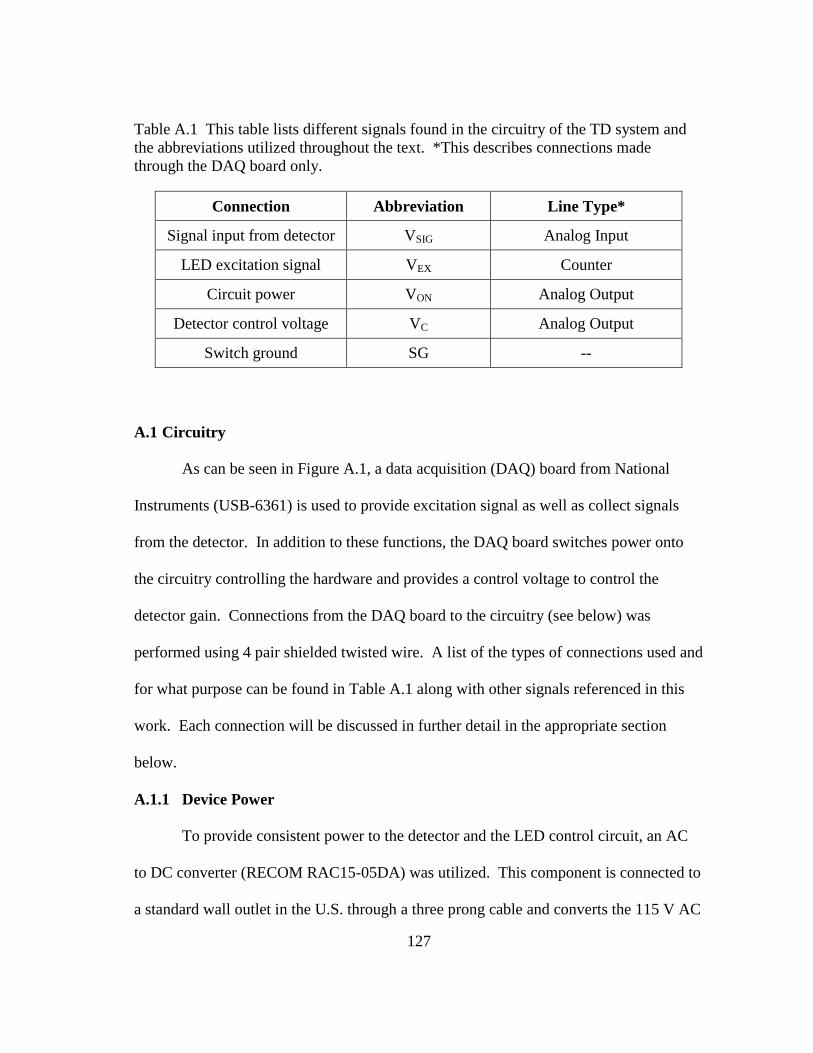
127
A.1 Circuitry
As can be seen in Figure A.1, a data acquisition (DAQ) board from National
Instruments (USB-6361) is used to provide excitation signal as well as collect signals
from the detector. In addition to these functions, the DAQ board switches power onto
the circuitry controlling the hardware and provides a control voltage to control the
detector gain. Connections from the DAQ board to the circuitry (see below) was
performed using 4 pair shielded twisted wire. A list of the types of connections used and
for what purpose can be found in Table A.1 along with other signals referenced in this
work. Each connection will be discussed in further detail in the appropriate section
below.
A.1.1 Device Power
To provide consistent power to the detector and the LED control circuit, an AC
to DC converter (RECOM RAC15-05DA) was utilized. This component is connected to
a standard wall outlet in the U.S. through a three prong cable and converts the 115 V AC
Table A.1 This table lists different signals found in the circuitry of the TD system and
the abbreviations utilized throughout the text. *This describes connections made
through the DAQ board only.
Connection Abbreviation Line Type*
Signal input from detector VSIG Analog Input
LED excitation signal VEX Counter
Circuit power VON Analog Output
Detector control voltage VC Analog Output
Switch ground SG --

128
to ±5 V DC. For this device, only the +5 V signal is utilized. A 2A fuse is also included
on the input to protect against power surges as suggested by the manufacturer.
To give power to the custom circuitry utilized by the system, a common NPN
transistor (2N3904) was utilized as seen in Figure A.2. When power is applied to VON
Figure A.2 This circuit shows the use of a common transistor as a switch to turn power
on and off to the remaining circuits.
Figure A.3 This circuit is used to drive the LED and ensures that the on/off speed is
much faster than the lifetimes measured.

129
through the DAQ board, the transistor is saturated allowing the rest of the circuit to be
grounded through SG.
A.1.2 Excitation Circuit
To drive power to the LED, a fast digital drive circuit was utilized similar to one
previously described where the capacitors in the circuit are utilized to improve the on/off
speeds of the LED (Figure A.3).227
This is needed in order to make the edges of the
square wave used for excitation as sharp as possible. Ground for the circuit is again
provided by the switch circuit shown in Figure A.2.
A.1.3 Detector Connections
The connections made for the detector can be seen in Figure A.4. The
decoupling capacitors shown on the control voltage and input power serve to reduce any
noise present on these lines. The 100 Ω resistor is needed to convert the current signal
output from the detector into a voltage signal that is measurable by the DAQ board on
VSIG.
A.2 Optical Components
Although this system is utilized to measure optical responses of luminescent
materials, only two parts of the device utilize optical components. The optical
components are used for excitation of the luminophore and detection of luminescence
following excitation. These two sections are coupled to the sample of interest through a
custom 2x1 fiber bundle (CeramOptec Industries, Inc.).
A.2.1 Excitation Signal
For the luminescence measurement of porphyrin responses, green excitation (525

130
nm) is often utilized. In order to improve the LED intensity at the sample, a series of
lenses with appropriate anti-reflection coatings were used to focus light from the LED
onto the fiber bundle. The parts utilized can be found in Table A.2.
A.2.2 Emission and Collection
Similar to the optics utilized for excitation of the sample, lenses were utilized to
focus light from the fiber bundle onto the detector and increase efficiency. Anti-
reflective coatings for the appropriate wavelengths were again utilized for the spherical
lenses. In addition, an optical longpass filter was implemented to ensure that any
Figure A.4 The connections including decoupling capacitors and a resistor for current-
to-voltage conversion for the detector are depicted above.
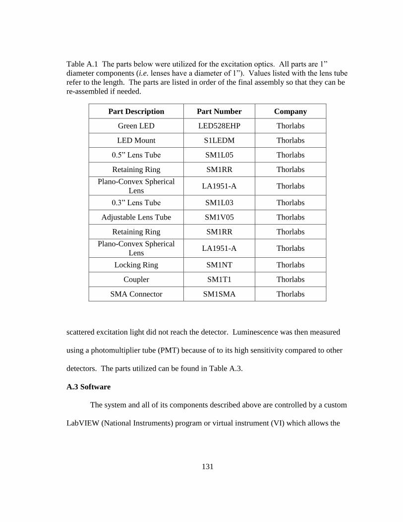
131
scattered excitation light did not reach the detector. Luminescence was then measured
using a photomultiplier tube (PMT) because of to its high sensitivity compared to other
detectors. The parts utilized can be found in Table A.3.
A.3 Software
The system and all of its components described above are controlled by a custom
LabVIEW (National Instruments) program or virtual instrument (VI) which allows the
Table A.1 The parts below were utilized for the excitation optics. All parts are 1”
diameter components (i.e. lenses have a diameter of 1”). Values listed with the lens tube
refer to the length. The parts are listed in order of the final assembly so that they can be
re-assembled if needed.
Part Description Part Number Company
Green LED LED528EHP Thorlabs
LED Mount S1LEDM Thorlabs
0.5” Lens Tube SM1L05 Thorlabs
Retaining Ring SM1RR Thorlabs
Plano-Convex Spherical
Lens LA1951-A Thorlabs
0.3” Lens Tube SM1L03 Thorlabs
Adjustable Lens Tube SM1V05 Thorlabs
Retaining Ring SM1RR Thorlabs
Plano-Convex Spherical
Lens LA1951-A Thorlabs
Locking Ring SM1NT Thorlabs
Coupler SM1T1 Thorlabs
SMA Connector SM1SMA Thorlabs
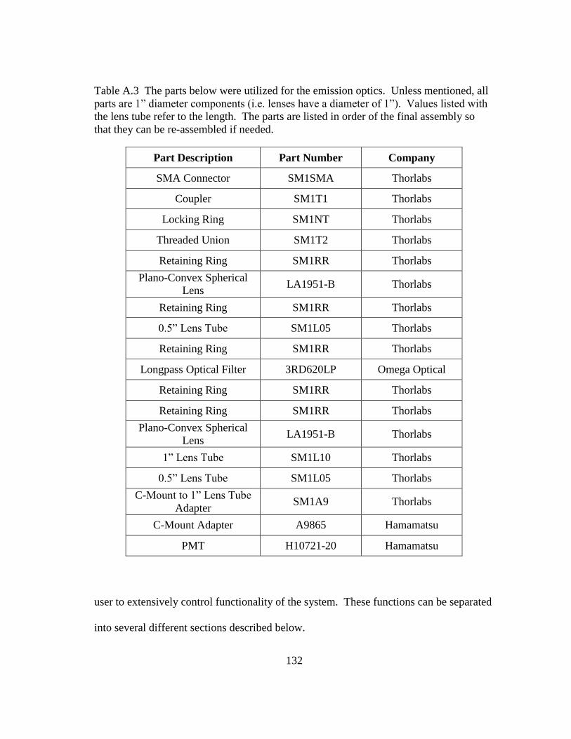
132
user to extensively control functionality of the system. These functions can be separated
into several different sections described below.
Table A.3 The parts below were utilized for the emission optics. Unless mentioned, all
parts are 1” diameter components (i.e. lenses have a diameter of 1”). Values listed with
the lens tube refer to the length. The parts are listed in order of the final assembly so
that they can be re-assembled if needed.
Part Description Part Number Company
SMA Connector SM1SMA Thorlabs
Coupler SM1T1 Thorlabs
Locking Ring SM1NT Thorlabs
Threaded Union SM1T2 Thorlabs
Retaining Ring SM1RR Thorlabs
Plano-Convex Spherical
Lens LA1951-B Thorlabs
Retaining Ring SM1RR Thorlabs
0.5” Lens Tube SM1L05 Thorlabs
Retaining Ring SM1RR Thorlabs
Longpass Optical Filter 3RD620LP Omega Optical
Retaining Ring SM1RR Thorlabs
Retaining Ring SM1RR Thorlabs
Plano-Convex Spherical
Lens LA1951-B Thorlabs
1” Lens Tube SM1L10 Thorlabs
0.5” Lens Tube SM1L05 Thorlabs
C-Mount to 1” Lens Tube
Adapter SM1A9 Thorlabs
C-Mount Adapter A9865 Hamamatsu
PMT H10721-20 Hamamatsu

133
A.3.1 Excitation Signal Control
The parts of the excitation signal provided to the sample that can be controlled
include the excitation frequency, duty cycle, number of decays collected, and the period
between measurements. The excitation frequency controls how fast the excitation pulses
of the square wave occur during measurement. The duty cycle refers to the amount of
time the LED is on relative to the excitation period. It should be noted that the time the
LED is on should be long enough to allow the luminescence to reach steady state to
improve the signal-to-noise ratio (SNR) of the decays. Also, the length of data
collection is typically a fraction of the time that the LED is off. Longer sampling will
not help because the signal will decay to zero. To further improve the SNR of the
luminescence decay, multiple decays were often collected and summed for a single
lifetime calculation. The measurement period must be greater than the number of decays
collected divided by the excitation frequency in order to prevent overworking of the
computer. A depiction of these parameters can be found in Figure A.5.
A.3.2 Data Acquisition
The start of data collection for each decay is timed through the software to begin
when the clock pulse used for excitation turns the LED off. Through the software, the
user is able to control the sampling frequency and the acquisition time. The sampling
frequency will be limited by the specifications of the DAQ board which in this case is 2
MHz. The acquisition time, however, will be limited by the amount of time the LED is
off which is dependent on the excitation frequency and the duty cycle.
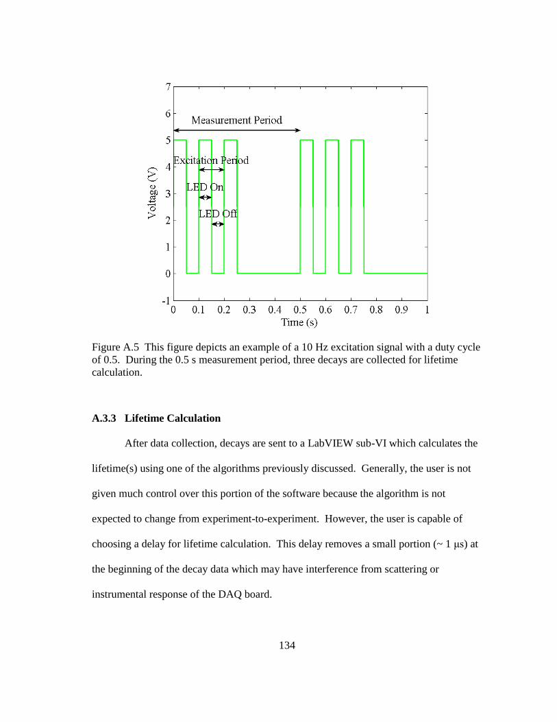
134
A.3.3 Lifetime Calculation
After data collection, decays are sent to a LabVIEW sub-VI which calculates the
lifetime(s) using one of the algorithms previously discussed. Generally, the user is not
given much control over this portion of the software because the algorithm is not
expected to change from experiment-to-experiment. However, the user is capable of
choosing a delay for lifetime calculation. This delay removes a small portion (~ 1 μs) at
the beginning of the decay data which may have interference from scattering or
instrumental response of the DAQ board.
Figure A.5 This figure depicts an example of a 10 Hz excitation signal with a duty cycle
of 0.5. During the 0.5 s measurement period, three decays are collected for lifetime
calculation.

135
A.3.4 Data Storage
Following data collection, the lifetimes calculated and any other appropriate
information such as time of measurement are written to a spreadsheet file for later
analysis.

136
CUSTOM TESTING BENCH APPENDIX B.
Oftentimes, the response to of luminescent sensors needs to be characterized for
a variety of environmental conditions. Usually this entails testing at a range of analyte
concentrations. In order to simplify data collection, automated test benches are often
utilized. These systems are pre-programmed by a user to expose the sensors to the
desired conditions while the response is recorded and saved for later data analysis.
Ultimately, this saves time because the user does not need to be present to constantly
monitor the response of the sensor or manually change the environment.
A general overview is provided for the test benches utilized in this and previous
works (Figure B.1).30-31, 152-153
This includes control of three environmental conditions
(glucose and oxygen concentration as well as temperature) and the measurement system.
Figure B.1 A general diagram of the test-bench is shown with glucose, oxygen, and
temperature control. A computer with custom software (not shown) is used to control
the MFCs, pumps, incubator, and the lifetime measurement system.
137
Control of the system was again performed using custom LabVIEW software (National
Instruments). Initially, programs were developed for each environmental element and
the measurement system. After validation, these programs were combined to create a
single program which encompassed the function of each. The sections below describe
the hardware and software used for each environmental entity. Details of the
measurement system can found in Appendix A.
B.1 Glucose Concentration Control
As seen in Figure B, control of glucose concentration requires two reservoirs
usually containing a phosphate-buffered saline solution. One reservoir also contains
glucose at the maximum concentration of interest. Using a pump for each reservoir,
solutions from each reservoir are combined to obtain the glucose concentration of
interest. This is done by holding the total flow rate constant while varying the flow rate
from each reservoir. For example, in order to get a concentration of 100 mg/dL for a
reservoir concentration of 400 mg/dL and a total flow rate of 4 mL/min the buffer pump
is run at 3 mL/min while the glucose pump is run at 1 mL/min. The concentrations
available will be dependent on the resolution of the pumps as well as the maximum and
minimum flow rates.
Three different kinds of pumps have been used in the past with this system.
Initially, peristaltic pumps (Cole Parmer, Masterflex 7550-50 and 77800-60) were
utilized, however, due to the need for frequent calibration, new pumps were sought.
Positive displacement piston pumps (VICI Valco Instruments Co., M50) were then
integrated into the system to overcome the issue of constant calibration and provide a
138
much higher resolution. However, the stainless steel parts and the PBS solutions utilized
are not very compatible for long-term use without rinsing frequently. The third set of
pumps (KNF, STEPDOS 03RC) were utilized positive displacement but with a
diaphragm mechanism. Although, they do not provide the resolution as the piston
pumps, they have a higher chemical inertness for use with PBS solutions.
Solutions were pumped through standard 1/8” tubing using ¼”-28 threaded
ferrules (IDEX Health and Science) and the appropriate adapters when needed. The
sensor being tested was immobilized on a glass slide and placed in a custom reaction
chamber that contained ports for the tubing coming from the supply reservoirs and out to
a waste reservoir. When the chamber was sealed a channel was formed between the top
of the chamber and the glass slide using a gasket. This channel allowed solution to flow
from the supply over the sensor and out to the waste. The chamber also has a port on the
bottom for a fiber optic bundle (see Appendix A) to allow interrogation of the sensor.
All three sets of pumps were controlled through USB connections on the computer and
LabVIEW software. The software utilized the Virtual Instrument Software
Archietecture (VISA) in conjunction with the driver functions provided by the
manufacturer for each pump. The functions utilized were able to start and stop the
pumps as well as set the flow rates which were calculated based on the desired glucose
concentration, total flow rate, and glucose reservoir concentration.
B.2 Oxygen Concentration Control
Control of oxygen concentration is provided in a similar fashion as that for
glucose. Rather than utilize liquid pumps, two mass flow controllers (MFCs, MKS
139
Instruments, 1179A) are used to control the flow of gas. Typically, compressed nitrogen
and air were supplied to each MFC, however, nitrogen and oxygen can be used for a
wider range of concentrations. The MFCs were controlled through an intermediate
controller (MKS Instruments, PR4000) which also provided power to the devices. Two
solenoid valves (Omega, SV3106) were placed inline before the MFCs because the
MFCs are not rated for use as valves only to control flow rate.
Using ¼” air brake tubing and the appropriate ferrules (Swagelok), gas was
flown into the supply reservoirs and dispersed using gas dispersion tubes (Chemglass,
CG-203-01) in the case of liquid testing. In the case of dry testing, the gas was allowed
to flow directly into to the reaction chamber. USB connections and VISA commands
were again used to control flow rates through the MFCs. The solenoids, however, were
controlled using a USB I/O Board (Phidgets, Inc., 1011_0) and a pair of relays (Omega,
SSRL240AC10). Using LabVIEW and the digital outputs of the I/O Board, the
appropriate relays are switched on or off as needed using the AC voltage from a standard
U.S. wall outlet. Software provided by Phidgets, Inc. was modified in order to control
the digital outputs.
Dissolved oxygen concentrations can be monitored in the reservoir using an
amperometric oxygen sensor (PA2000, Unisense). This will ensure that the system is
working as desired and allow measurements of the actual oxygen concentration to be
made for calibration purposes, if necessary. A two point calibration using air and
nitrogen or some other inert gas is required for this device.

140
B.3 Temperature Control
Temperature control of the system was more straightforward than the other
environmental elements. This was done by placing the reaction chamber inside of a
programmable incubator (Torrey Pines Scientific, IN35). A port on the side of the
incubator was necessary to allow tubing for the solutions and the fiber bundle to connect
to the reaction chamber. The incubator was connected to a USB port on the computer
and controlled through a VISA interface in LabVIEW. It is important to note that while
glucose and oxygen concentrations can be changed almost instantaneously, it takes much
more time for the incubator to reach steady-state and even more time for the reaction
chamber to reach that temperature throughout.
B.4 Miscellaneous
In case of power outages, most components were connected to an uninterruptible
power supply (UPS) which will provide power for a period of time. This will help
prevent the loss of data and time since tests run using this system can take several hours
to several days depending on the experiment.

141
LIFETIME CALCULATION SOURCE CODE APPENDIX C.
On the following pages, the MATLAB source code for both single and dual
dynamic rapid lifetime determination is included. Commented lines not part of the
function of the code begin with a percent symbol (“%”). Each lifetime calculation
function begins with a comment section that describes the functions purpose, the inputs
required, and the outputs received.
C.1 Dynamic Rapid Lifetime Determination Source Code
% ------------------------------------------------------------------------- % DRLD.m % Calculates lifetime and pre-exponential factor of a luminescence decay % % Syntax: % % [tau k] = DRLD(t, int, w1_delay, w_width1) % % Inputs: % t = time array of decay % int = time-dependent intensity array of decay % w1_delay = initial time-delay before windows are implemented % (utilized to throw out back-scattered light or auto-fluorescence) % w_width1 = initial window width utilized % % Outputs: % tau = calcualted mono-exponential lifetime of decay provided % k = calculated pre-exponential factor of decay provided % ------------------------------------------------------------------------- function [tau k] = DRLD(t, int, w1_delay, w_width1) ts = 1e-6; %magnitude of time array, in this case microseconds (1e-6) fs = 2e6; %sampling frequency of time-array, 1/fs gives time resolution %which is 0.5 microseconds in this case w_scale = 1.5; %factor by which to scale windows to calculate lifetime range1 = 2.7; %acceptable range of window sum ratios

142
range2 = 7.4; %convert initial window width from time to next highest indexed value %if not equal w_width1_i = ceil(w_width1*ts*fs); %convert window delay from time value to next highest indexed value %if not equal w1_delay_i = ceil(fs*w1_delay*ts)+1; %max window set based on length of time array and window delay previously %determined max_window_i = floor((length(t)-w1_delay_i)/2); %makes sure initial width selected is not larger than max width allowed w_width1_i = min(max_window_i, w_width1_i); %max number of iterations allowed before stopping, prevents infinite loops max_loop = 10; %initialize iterations number to zero i = 0; %loop performed until the ratio of window sums is within the desired %or another ending condition is met while(true) %increment the iteration number i=i+1; %determine the start and end times for window (in indices, not time) t1 = w1_delay_i; t2 = w_width1_i+w1_delay_i; t3 = 2*w_width1_i+w1_delay_i; %calculate the window sums for each window and the ratio w1 = sum(int(t1:t1+w_width1_i)); w2 = sum(int(t2:t2+w_width1_i)); R = w1./w2; %determine the window width in time value dif1 = w_width1_i/fs; %calculate the lifetime using RLD equation tau = abs((dif1)/log(R)); %checks if max loop # reached or R within desired range

143
if( (i >= max_loop) || ( (R >= range1) && (R <= range2) ) ) %exit loop break; %checks for negative R value indicative of windows being too long elseif(R < 0) % cut window length in half w_width1_i = floor(w_width1_i/2); %check if window has reached max width but needs to be larger in order %to reach optimal width elseif((R < range2)&&(w_width1_i == max_window_i)) %exit loop because cannot improve further break; else %adjust window width based to estimated optimal value or max w_width1_i = min([floor(fs*w_scale*tau), max_window_i]); end end %determine actual window delay using time value t1 = t1/fs; %calculate pre-exponential factor using calculated lifetime, window delay, %and sampling frequency k = w1/(tau*(1-1/R)*exp(-t1/tau))/fs; %convert lifetime to appropriate magnitude tau = tau/ts;
C.2 Dual Dynamic Rapid Lifetime Determination Source Code
% ------------------------------------------------------------------------- % DDRLD.m % Calculates lifetimes and pre-exponential factors of a dual-exponential % luminescence decay of the form I(t) = k1*exp(-t/tau1)+k2*exp(-t/tau2) % where k1 and tau1 refer to the lifetime and pre-exponential factor of % the shorter-lived dye, and k2 and tau2 refer to the same parameters of % the longer-lived dye % % Syntax:
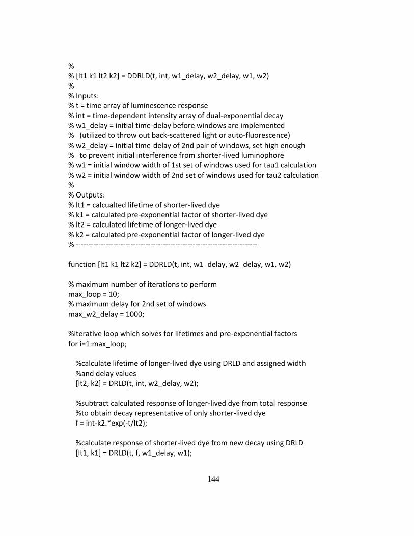
144
% % [lt1 k1 lt2 k2] = DDRLD(t, int, w1_delay, w2_delay, w1, w2) % % Inputs: % t = time array of luminescence response % int = time-dependent intensity array of dual-exponential decay % w1_delay = initial time-delay before windows are implemented % (utilized to throw out back-scattered light or auto-fluorescence) % w2_delay = initial time-delay of 2nd pair of windows, set high enough % to prevent initial interference from shorter-lived luminophore % w1 = initial window width of 1st set of windows used for tau1 calculation % w2 = initial window width of 2nd set of windows used for tau2 calculation % % Outputs: % lt1 = calcualted lifetime of shorter-lived dye % k1 = calculated pre-exponential factor of shorter-lived dye % lt2 = calculated lifetime of longer-lived dye % k2 = calculated pre-exponential factor of longer-lived dye % ------------------------------------------------------------------------- function [lt1 k1 lt2 k2] = DDRLD(t, int, w1_delay, w2_delay, w1, w2) % maximum number of iterations to perform max_loop = 10; % maximum delay for 2nd set of windows max_w2_delay = 1000; %iterative loop which solves for lifetimes and pre-exponential factors for i=1:max_loop; %calculate lifetime of longer-lived dye using DRLD and assigned width %and delay values [lt2, k2] = DRLD(t, int, w2_delay, w2); %subtract calculated response of longer-lived dye from total response %to obtain decay representative of only shorter-lived dye f = int-k2.*exp(-t/lt2); %calculate response of shorter-lived dye from new decay using DRLD [lt1, k1] = DRLD(t, f, w1_delay, w1);

145
%adjust delay of 2nd set of window to improve lifetime accuracy of both %lifetimes w2_delay2 = min([5*lt1 max_w2_delay]); %if the delay does not change, optimal window widths and delays %reached, break from loop if(w2_delay2==w2_delay) break; end %assign new delay value for next iteration w2_delay = w2_delay2; end