ISA Transactions 52 (2013) 19–29

Contents lists available at SciVerse ScienceDirect

ISA Transactions

0019-05

http://d

n Corr

E-m

vadlam

harekris1 Te

journal homepage: www.elsevier.com/locate/isatrans

Development and comparison of neural network based soft sensorsfor online estimation of cement clinker quality

Ajaya Kumar Pani n, Vamsi Krishna Vadlamudi, Hare Krishna Mohanta 1

Department of Chemical Engineering, Birla Institute of Technology and Science, Pilani 333031, India

a r t i c l e i n f o

Article history:

Received 5 March 2012

Received in revised form

8 June 2012

Accepted 11 July 2012Available online 31 August 2012

This paper was recommended

for publication by Ricky Dubay

Keywords:

Cement kiln modeling

Back propagation neural network

Radial basis function neural network

Regression neural network

Soft sensor

78/$ - see front matter & 2012 ISA. Published

x.doi.org/10.1016/j.isatra.2012.07.004

esponding author. Tel.: þ91 9929832108.

ail addresses: akpani@bits-pilani.ac.in (A.K. Pa

udiy5ch845@gmail.com (V.K. Vadlamudi),

hna.mohanta@gmail.com (H.K. Mohanta).

l.: þ91 9829434948.

a b s t r a c t

The online estimation of process outputs mostly related to quality, as opposed to their belated

measurement by means of hardware measuring devices and laboratory analysis, represents the most

valuable feature of soft sensors. As of now there have been very few attempts for soft sensing of cement

clinker quality which is mostly done by offline laboratory analysis resulting at times in low quality

clinker. In the present work three different neural network based soft sensors have been developed for

online estimation of cement clinker properties. Different input and output data for a rotary cement

kiln were collected from a cement plant producing 10,000 tons of clinker per day. The raw data were

pre-processed to remove the outliers and the resulting missing data were imputed. The processed data

were then used to develop a back propagation neural network model, a radial basis network model and

a regression network model to estimate the clinker quality online. A comparison of the estimation

capabilities of the three models has been done by simulation of the developed models. It was observed

that radial basis network model produced better estimation capabilities than the back propagation and

regression network models.

& 2012 ISA. Published by Elsevier Ltd. All rights reserved.

1. Introduction

A major problem in product quality control in process indus-tries is the difficulty faced in continuous online measurement ofcertain output variables especially related to composition.Although in some cases online analyzers are available, significanttime delays associated with most of such instruments maketimely control difficult and sometimes impossible. Moreoversuch instruments have low reliability. Soft sensing is a modelingapproach to estimate hard-to-measure process variables (primaryvariables) from easy-to-measure, online process variables(secondary variables). This plant model may be a first principlemodel, a black box model or a gray box model substituting somephysical sensors and using data acquired from some otheravailable ones. Though modeling of a process from first principlesis often desirable, in most cases however a first principle model isnot possible because of the enormous amount of complexityinvolved and/or the intensive computation works involved. Onthe other hand modern measurement techniques enable a largeamount of operating data to be collected, stored and analyzed,

by Elsevier Ltd. All rights reserve

ni),

thereby rendering data-driven modeling methods (black box orgray box) more preferable to first principles models for complexprocesses.

Artificial neural network (ANN) has been a popular empiricalmodeling technique over the years. The details of processes forwhich neural network modeling has been done is given under thecategory of each type of neural network development. Other thanpollutant emission studies, there have been very few attempts todevelop ANN based soft sensor for online estimation of productquality in cement plant. The quality of clinker plays the mostimportant role in determining the quality of cement. Unfortu-nately there is no hardware sensor available for online sensing ofclinker composition coming out of a rotary cement kiln. Theclinker quality is determined by measuring its contents of freelime and other important components by offline laboratoryanalysis. Therefore any reduction in clinker quality, as determinedby offline laboratory analysis hours after production, leads torejection or recycling of the clinker formed. Any method foronline estimation of clinker quality will largely help in reducingthe amount of rejection thereby resulting in lower revenue loss ormore profit. A few works on kiln modeling has been done basedon statistical approach [1,2]. However these works are aimed onlyat estimating the free lime content of the clinker. While free limecontent is the most important clinker quality parameter, there arealso other important quality parameters (mentioned later in thepaper) which require online estimation for better product quality.

d.

Nomenclature

ci ith RBF centerDi

2 Euclidean distance between two input vectorsIj Input to jth pattern neuron of GRNNn Number of training samplesQ0.25, Q0.75 1st and 3rd quartile value of a datasetvar(y) Variance of a dataset y

wi Weight associated with ith RBF centerwij Weight associated with ith input neuron and jth

pattern neuronxi ith observation value of an input variable

x Mean value of a data setx0.5 Median value of a data setxmax Maximum value of a variable in a datasetxmin Minimum value of a variable in a datasetxnorm Normalized valuey Actual output value (normalized)y Simulated output value of neural network models Standard deviation, scaling parameter of RBF net-

work, spread coefficient in GRNNg Skewness of a data setk Kurtosis of a data setji RBF model basis function

A.K. Pani et al. / ISA Transactions 52 (2013) 19–2920

In the present work neural network based soft sensors havebeen developed for estimation of eight clinker quality parameters.Three types of network models, a back propagation network model,a radial basis function network model and a regression networkmodel, have been developed and a comparison of their perfor-mances has been done. The models receive four raw mix qualityparameters and five physical variables pertaining to kiln operationi.e. rpm, current, fuel flow rate, temperature and kiln feed rate asinputs and produce values of eight clinker quality parameters.

The article describes the following topics in order: briefdescription of the cement making process with focus on therotary cement kiln, data preprocessing, neural network develop-ment, simulation results, discussion and conclusion.

2. Brief description of cement manufacturing process

The raw materials for cement are limestone as a source of lime,clay as a source of silica, laterite as a source of iron and red ochreas a source of aluminum. These raw materials are first mixed inthe required proportion which is referred to as raw meal. This rawmeal is then ground to required size in a vertical roller mill. Therequired size raw meal then enters a multistage cyclone preheaterwhere it is preheated by the hot flue gas coming from the cementrotary kiln. Bulk of the calcination (CaCO3-CaOþCO2) of the rawmeal is done in the multistage cyclone preheater. The preheatedraw meal then enters the cement kiln. The rotary kiln is the heartof the cement plant where the different components present inthe raw meal, at high temperature, react with each other.The lime (CaO) reacts with other components like silica, aluminaand iron oxide present in the raw meal to form complexesof dicalcium silicate (C2S), tricalcium silicate (C3S), tricalcium

Table 1All associated variables for cement kiln.

Raw meal quality Clinker quality

SiO2, Al2O3, Fe2O3, CaO, MgO, K2O, Na2O, SO3, Cl, Lime

Saturation Factor, Silica Modulus, Alumina Modulus

SiO2, Al2O3, Fe2O3, CaO, MgO

saturation Factor, Silica Mod

Table 2Final selected variables for the cement kiln.

Raw meal quality Clinker quality

SiO2, Al2O3, Fe2O3, CaO, Free Lime, Lime Saturation Factor,

Alumina Modulus, C3S, C2S, C3A, C

aluminate (C3A) and tetracalcium aluminoferrite (C4AF). All thesecomponents must be maintained in a required proportion in theclinker for maintaining the quality. The unreacted lime appears asfree lime in the clinker which should be limited to a minimum.The clinker is then ground with a small amount of gypsum in thecement mill producing the final product i.e. cement.

In the cement plant the quality of the clinker to a large extentaffects the quality of the cement. However this clinker quality ismostly determined by offline laboratory analysis by taking clinkersamples at kiln outlet at regular intervals and then analyzing thesame for different components. Therefore failure to meet thequality criteria leads to the rejection/recycling of the kiln productresulting in significant revenue loss. So a soft sensor which iscapable of continuous online estimation of clinker compositioncan minimize the occurrence of such problems.

In order to develop the data driven soft sensor, data werecollected over a period of one month for various quality para-meters of the raw meal as well as corresponding output clinkerand kiln operating variables from a cement plant having a kilncapacity of 10,000 t clinker per day as shown in Table 1.

3. Data preprocessing

An industrial database provides data of all the variables thatare recorded. In the present work as shown in Table 1, there are12 variables pertaining to raw meal quality (kiln inlet), 5 kilnoperating variables and 17 clinker quality variables. Out of allquality parameters of clinker, eight important parameters werechosen to be predicted by the model. For prediction of a fewchosen quality parameters, all the input information is notrequired. Presence of irrelevant (or less relevant) variable data

Kiln operating variables

, K2O, Na2O, SO3, Cl, Free Lime, lime

ulus, Alumina Modulus, C3S, C2S, C3A, C4AF

Kiln feed rate, current, kiln RPM,

feed inlet temperature, coal feed

rate

Kiln operating variables

Silica Modulus,

4AF

Kiln feed rate, current, kiln RPM,

feed inlet temperature, coal feed rate

A.K. Pani et al. / ISA Transactions 52 (2013) 19–29 21

in the input data set leads to noise which may result in thedeterioration of the model. For neural network modeling, a reduc-tion in the input data dimension leads to simplified neural archi-tecture and reduced training time [3]. One approach to reducing theinput variable dimension is by applying statistical methods such asprincipal component analysis (PCA) or partial least squares (PLS)which results in a low dimension input space. However the problemassociated with such methods are the new variables which are acombination of the original variables, are difficult to interpret interms of actual process variables [4]. Therefore based on priorprocess knowledge and in consultation with plant operators thevariables shown in Table 2 were retained for subsequent modeldevelopment. The raw meal quality parameters along with the kilnoperating variables are the inputs for the kiln model and the clinkerquality parameters are the outputs of the model.

The next task is handling of outliers and missing data. Theseproblems are more likely to take place in case of online measure-ment than laboratory measurement. Outliers are sensor valueswhich deviate from the typical, or sometimes also meaningful,ranges of the measured values. The raw data extracted from theplant database are often contaminated with outliers which mighthave resulted due to one or more reasons of hardware failure,process disturbances or changes in operating conditions, instru-ment degradation, transmission problems and/or human error [1].Outliers may lead to model misspecification, biased parameterestimation and incorrect analysis results [5].

In this work also, the collected industrial data suffers fromproblem of outliers as shown in Fig. 1. Three popular outlier

Fig. 1. Actual online data of ceme

Table 3Skewness and kurtosis values for raw and treated data.

Kiln operating

parameters

Value for raw data Value for tre

3 sigma

g k g

Kiln feed rate �3.842 18.442 �3.79

Kiln current 32.946 1105.4 �7.318

Kiln RPM �3.141 13.673 �2.50

Kiln feed inlet temperature 9.954 110.73 14.341

Coal feed rate 34.577 1196.7 �3.862

detection techniques [6,7], the 3s method, Hampel’s method andthe Box plot method were applied to each of the online operatingvariable data set. The 3s method detects the data values asoutliers satisfying the following inequality:

9xi�x9s 43 ð1Þ

The same for Hampel’s method is presented in Eq. (2).

9xi�x0:591:4826�median9xi�x0:59

43 ð2Þ

In the box plot method, the different regions in the plot aredefined as

Lower inner fence : Q0:25�1:5� Q0:752Q0:25ð Þ

Upper inner fence : Q0:75þ1:5� Q0:752Q0:25ð Þ

Lowerouterfence : Q0:25�3� Q0:752Q0:25ð Þ

Upperouterfence : Q0:75þ3� Q0:752Q0:25ð Þ

9>>>>=>>>>;

ð3Þ

Q0.25 and Q0.75 are 25% and 75% quantiles respectivelyA mild outlier is a point beyond an inner fence on either side

while an extreme outlier is a point beyond an outlier fence.The performance of the three techniques were evaluated by

determining the skewness and kurtosis values for the dataobtained after the removal of outliers by a particular technique.The skewness value of a data set is defined as

g¼P

xi�xð Þ3

ns3ð4Þ

nt kiln operating parameters.

ated data

Hampel’s method Box plot rule

k g k g k

19.119 �1.181 4.12 �1.669 5.658

75.024 �0.056 2.676 0.068 4.716

9.497 �1.317 3.9231 �1.892 6.2741

227.488 �0.624 3.51 �1.038 4.70

21.554 �0.671 4.321 �1.429 6.47

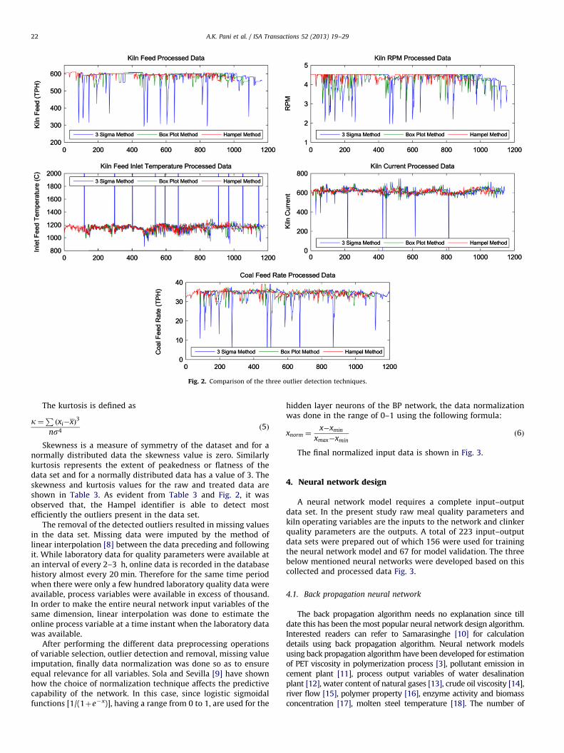
Fig. 2. Comparison of the three outlier detection techniques.

A.K. Pani et al. / ISA Transactions 52 (2013) 19–2922

The kurtosis is defined as

k¼P

xi�xð Þ3

ns4ð5Þ

Skewness is a measure of symmetry of the dataset and for anormally distributed data the skewness value is zero. Similarlykurtosis represents the extent of peakedness or flatness of thedata set and for a normally distributed data has a value of 3. Theskewness and kurtosis values for the raw and treated data areshown in Table 3. As evident from Table 3 and Fig. 2, it wasobserved that, the Hampel identifier is able to detect mostefficiently the outliers present in the data set.

The removal of the detected outliers resulted in missing valuesin the data set. Missing data were imputed by the method oflinear interpolation [8] between the data preceding and followingit. While laboratory data for quality parameters were available atan interval of every 2–3 h, online data is recorded in the databasehistory almost every 20 min. Therefore for the same time periodwhen there were only a few hundred laboratory quality data wereavailable, process variables were available in excess of thousand.In order to make the entire neural network input variables of thesame dimension, linear interpolation was done to estimate theonline process variable at a time instant when the laboratory datawas available.

After performing the different data preprocessing operationsof variable selection, outlier detection and removal, missing valueimputation, finally data normalization was done so as to ensureequal relevance for all variables. Sola and Sevilla [9] have shownhow the choice of normalization technique affects the predictivecapability of the network. In this case, since logistic sigmoidalfunctions [1/(1þe�x)], having a range from 0 to 1, are used for the

hidden layer neurons of the BP network, the data normalizationwas done in the range of 0–1 using the following formula:

xnorm ¼x�xmin

xmax�xminð6Þ

The final normalized input data is shown in Fig. 3.

4. Neural network design

A neural network model requires a complete input–outputdata set. In the present study raw meal quality parameters andkiln operating variables are the inputs to the network and clinkerquality parameters are the outputs. A total of 223 input–outputdata sets were prepared out of which 156 were used for trainingthe neural network model and 67 for model validation. The threebelow mentioned neural networks were developed based on thiscollected and processed data Fig. 3.

4.1. Back propagation neural network

The back propagation algorithm needs no explanation since tilldate this has been the most popular neural network design algorithm.Interested readers can refer to Samarasinghe [10] for calculationdetails using back propagation algorithm. Neural network modelsusing back propagation algorithm have been developed for estimationof PET viscosity in polymerization process [3], pollutant emission incement plant [11], process output variables of water desalinationplant [12], water content of natural gases [13], crude oil viscosity [14],river flow [15], polymer property [16], enzyme activity and biomassconcentration [17], molten steel temperature [18]. The number of

Table 4BPNN details.

No of input nodes 9

No of output nodes 8

No of hidden layers 2

No of neurons in 1st hidden layer 9

No of neurons in 2nd hidden layer 12

Activation function for the two hidden layers Sigmoidal

Activation function for output layer Linear

Training algorithm used Scaled conjugate gradient

A.K. Pani et al. / ISA Transactions 52 (2013) 19–29 23

neurons in the input layer and the hidden layer are the same as thenumber of input variables and output variables of the process.Choosing the number of hidden layers and number of neurons ineach hidden layer is the most critical decision to a successful design ofBPNN. Unfortunately there is no universal method to determine theoptimum network topology and these are mostly decided based on atrial and error procedure so as to produce the least error [3,13,19].Usually a single hidden layer is used to solve functional approxima-tion problems and if the performance goal is not attained in a singlehidden layer gradually the number of hidden layers can be increased.The more the number of hidden layers the more is the complexityassociated and large is the training time required. Few number ofneurons in the hidden layer leads to poor model accuracy whereasmany number of neurons result in model over fitting and poorgeneralization. In the present work however the use of two hiddenlayers produced significantly less error as compared to the use of onlyone hidden layer. The number of neurons was determined byconducting model training for different numbers of neurons rangingfrom 3 to 20 and choosing the one producing the least error. The finaloptimum architecture based on large number of simulations is givenin Table 4 and the figure is produced in Fig. 4.

4.2. RBF neural network

Multilayer feed forward networks with sigmoidal activationfunctions have been proven to be universal approximatorswhich are mostly trained by the back propagation method usinggradient descent algorithm. However, the disadvantages of BP neuralnetworks are the following [20–22]: excessive computational or

Fig. 3. Final processed data to be

training time due to the use of non-linear optimization techniques,and the possibility of getting trapped in local minima resulting insub-optimal solution. Although the use of genetic algorithm mayresult in global minima, the procedure is computation intensive.

Radial basis function networks are a class of feed forwardsupervised networks. It is a two layer network consisting of an inputlayer, a hidden layer and an output layer with linear parameters.Non-linear basis functions are used at the hidden layer neurons. Acenter is associated with every hidden layer node. Hidden layer nodescalculate the Euclidean distance between the center and the inputvector which is sent as an input to the basis function. The differenttypes of basis functions used are as follows [20]:

Thin plate spline function : j xð Þ ¼ x2 logðxÞ ð7Þ

Gaussian function : j xð Þ ¼ exp �x2

s2

� �ð8Þ

used for model development.

Fig. 4. Back propagation neural network architecture.

A.K. Pani et al. / ISA Transactions 52 (2013) 19–2924

Normalised Gaussian function ji xð Þ ¼exp �:x�ci:

2=s2

i

� �Pn

j ¼ 1 exp �:x�cj:2=s2

j

� � ð9Þ

Multiquadratic function : j xð Þ ¼ x2þs2� �1=2

ð10Þ

Inverse multiquadratic function : j xð Þ ¼ x2þs2� ��1=2

ð11Þ

s is the scaling parameter or the width which controls the spread ofthe function around the center.

Out of the above functions, the Gaussian type is mostly used asactivation function for hidden layer nodes. So for an input vectorx, the network output is given as

y¼ f xð Þ ¼Xn

i ¼ 1

wijð:x�ci:Þ ð12Þ

wt is the weight associated with ith RBF center and :x�ci: is theEuclidean distance between center ci and the input vector x.

The linear parameters used in RBF networks result in fastertraining and less convergence problems in comparison to BPneural networks. Also RBF networks have better approximationability with simpler network architecture as compared to MLPs[23]. Selection of an appropriate radial basis network requirescareful selection of basis function and their associated parameters(centers and widths). The performance of an RBF network largelydepends on the centers chosen. As a strict interpolator thenetwork must have as many RBF centers as the training data.However this results in a large structure when the data are plentyand results in over fitting of the data and poor generalizationcapability of the network. On the other hand the use of very lessnumber of centers results in under fitting of the data [24].

The centers and widths are obtained using k-means clusteringalgorithm or density estimation methods. This involves classify-ing the input data into k number of clusters. The cluster centersare determined by minimizing the total squared error incurred inrepresenting the data set by k cluster centers. However thedrawbacks of this standard algorithm are that for determiningthe hidden nodes many passes of all training data are requiredresulting in large computational time for large dataset [23].

Moreover, though this method has faster training but results inlocal optimum yielding suboptimal models [25,26].

The second category makes use of algorithms to determine thenetwork structure as well as the parameters. Some of the proposedalgorithms are orthogonal least squares algorithm [20,22], geneticalgorithm [27], individual training of each hidden unit based onfunctional analysis, fuzzy partition of input space followed by linearregression [23].

In the present work, a two layered feed forward neuralnetwork was constructed. The first layer has radial basis neuronswith Gaussian activation function as given in Eq. (8) to performthe non-linear transformation of the input signal.

The second layer has linear neurons which produce linearoutputs. The following iteration is performed until the network’smean squared error falls below goal or the maximum number ofneurons are reached:

(1)

The network is simulated with no neurons in the first layer. (2) The input vector with the greatest error is determined. (3) A radial basis neuron is added with weights equal to that vector. (4) The output layer weights are redesigned to minimize error.

In the present case the goal was set to zero and maximumnumber of neurons to 70. A larger spread smoothens the functionapproximation and a too small spread value leads to the use ofmore number of neurons to fit a smooth function. After adequatetrial and error an optimum spread value of 0.4 was used in thepresent case.

4.3. Generalized regression neural network

Generalized regression neural network (GRNN) which was firstproposed by Specht [28] is a powerful tool for non-linear functionapproximation. In the general regression algorithm, the form ofinput–output dependence is expressed as a probability densityfunction determined from the observed data. The algorithm has

A.K. Pani et al. / ISA Transactions 52 (2013) 19–29 25

the form [28]:

y¼

Pni ¼ 1 y� exp

�D2i

2s2

� �Pn

i ¼ 1 exp�D2

i

2s2

� � ð13Þ

Di2, the Euclidean distance between two input vectors is given as:

D2i ¼ xi�xj

� �Txi�xj

� �ð14Þ

The regression equations can be implemented in a neuralnetwork like structure which is then known as GRNN. Fig. 5shows the typical structure of a GRNN.

A typical GRNN has four layers: an input layer, a pattern layer,a summation layer and the output layer. Input layer has the samenumber of neurons as the number of input variables and patternlayer has the same number of neurons as the number of trainingcases. Pattern neurons compute a distance which is the square ofthe differences across all weights as described in Eq. (14). For jthpattern neuron, net input is

Ij ¼Xn

i ¼ 1

wij�xj

� �2ð15Þ

The activation function associated with the pattern neuron isexponential and can be written as expð�I2

j =2s2Þ. The choice ofsmoothing function or spread parameter s is critical to the successfuldesign of a GRNN. A large value of s results in more generalizationand smoother fitting whereas a low value results in more accuratefitting and poor generalization. The method suggested for optimumselection of s is the hold out or leave one out method [28,29]. Thesummation neurons calculate the sum of weighted inputs frompattern layer. There have been some applications of GRNN modelingfor estimation of crude oil viscosity [14], river flow [15], polymerproperty [16], soil quality [29], river sediments [30], coal grindability[31], plasma process parameters [32], water quality [33], compressivestrength and elasticity modulus [34], NOx emission [35].

5. Results

Hampel’s identifier, which uses outlier resistant median andmedian absolute deviation (MAD) values instead of the outliersensitive mean and standard deviation, is more effective. There-fore it can be concluded that if outlier numbers are less in a verylarge data set which will affect the values of mean and standarddeviation insignificantly one can use the three sigma method.Otherwise it is better to use the Hampel’s identifier.

Fig. 5. Generalized regression

The total collected data (online process variable data fromdatabase history and quality data from the laboratory), after outlierremoval, missing value imputation and data normalization, were splitinto two parts. Two thirds of the data (156 data values) were used formodel development (training data) and one third (67 data values)were used for model validation purpose. While selecting the data forneural network training, it was ensured that the highest and thelowest values from each variable set were retained in the training setso that the developed model can be used over a wider operatingrange. Because empirical models do not extrapolate well and oneshould be careful while using the model, the input data actually fallswithin the range which was used for model development.

Figs. 6 and 7 make a comparison of the estimation capability ofthe three neural network models with respect to the trained anduntrained data respectively. The performance of the models isdetermined by evaluating the mean of squared error (MSE) valuesproduced by each model to the trained and untrained data.

The MSE value is given as

Pni ¼ 1 y�y

� �2

nð16Þ

Table 5 shows the minimum mean squared error achieved forthe three models. Actual variable values are used for the graphswhereas the mean squared error values are based on the normal-ized values. Further analysis of the estimation capabilities of thedeveloped models was done by computing the variance account for(VAF) values of the models for the unknown data. The VAF valuesfor different estimated parameters are presented in Table 6.

6. Discussion

As stated earlier, the skewness and kurtosis values for anormally distributed data should be 0 and 3 respectively. Thereforeit can be concluded that the outlier detection technique producingskewness and kurtosis result close to these values is the mosteffective. From Table 3 the superiority of Hampel’s method over theother two methods is verified.

Training of the neural network can be viewed as a parameterestimation technique to get the best model. But before choosingthe model the following must be determined:

Does the model perform well with the untrained data?Is the best developed model suitable enough for a given

process application?The answer to the first question is the model validation

process which was carried out by simulating the model with

neural network structure.

Fig. 6. Actual and estimated values of clinker quality parameters for training data.

A.K. Pani et al. / ISA Transactions 52 (2013) 19–2926

unknown data and determining the error or residual valuebetween actual and model estimated values. The mean squarederror values produced by different models to validate the data isproduced in Table 5.

One interesting observation is, as far as simulation of thenetworks for the training data is concerned, all three modelsproduce almost comparable results (Fig. 6 and 2nd columnTable 5). But the important aspect where the BP network modellags behind the radial basis network and the regression networkmodel is the generalization capability of the models (Fig. 7 and3rd column Table 5) i.e. how well the models perform when theyare supplied with data not used for the training. As stated earlier

the optimum selection of the spread coefficient is crucial to thesuccess of the GRNN model. Theoretically, a decrease in the valueof sigma s will increase error value for untrained data (poorgeneralization) and decrease error value for trained data (overfitting). In this case, a decrease in s below the optimum value of4.9 resulted in decrease in MSE for trained data but increase inMSE for unknown data. However a value beyond the optimum didnot result in better generalization but only resulted in significantincrease in MSE for trained data.

It is quite obvious from Table 5 that RBFN and GRNN clearlyoutperform the network model trained by the back propagationmethod. The performance of a model is assessed by its ability for

Fig. 7. Actual and estimated values of clinker quality parameters for validation data.

Table 5Mean squared error comparison of neural network soft sensors.

Types of

Neural Network

Mean squared error

value for training data

Mean squared error

value for untrained data

Back propagation 0.0068 0.0693

Radial basis 0.0086 0.03

Generalized regression 0.0038 0.039

A.K. Pani et al. / ISA Transactions 52 (2013) 19–29 27

generalization. However there is only marginal error difference inthe validation process between RBFN and GRNN models. To havea clear answer to whether the best designed model is goodenough for the purpose, further analysis of the model perfor-mances were done by computing the variance account for (VAF)

[36] of the different models in predicting the clinker qualityparameters. The VAF is defined as

VAF ¼ 1�var y�y� �

var yð Þ

� � 100 ð17Þ

The closer is the value of VAF to 100, the better is the model.Detailed analysis of the results of Table 6 reveals that the BPNNmodel has very low generalization capability. The high negativeVAF values for the BPNN model is due to the fact that the modelexhibits highly erratic behavior in estimating outputs fromunknown inputs, resulting in much higher variance for the resi-duals (y�y) than for the actual output. Except free lime content, allother clinker quality parameters are better predicted by RBFN thanGRNN as evident by the higher VAF values for the RBFN model.

The final issue regarding online implementation of soft sensorsin the process has been discussed by several researchers [3,37].

Fig. 8. Online implementation of soft sensor.

Table 6VAF values for model simulated output for unknown input data.

Quality Parameters VAF values for different neural network models

BPNN RBFN GRNN

Free lime (FCaO) �981.634 54.612 67.457

Lime Saturation Factor (LSF) �1206.493 61.33 39.14

Alumina Modulus (ALM) �1648.77 66.134 46.457

Silica Modulus (SiM) �3321.1 39.7 29.06

C3S �3689.38 42.6 6.94

C2S �3281.34 43.14 14.06

C3A �2949.07 32.53 23.37

C4AF �3316.57 63.38 49.92

A.K. Pani et al. / ISA Transactions 52 (2013) 19–2928

A properly trained and validated soft sensor should be able tomake real time estimates of the clinker quality when suppliedwith the values of the kiln operating parameters as measured bythe physical hardware sensors and the raw mix quality values.The estimated clinker quality values then can be used by thecontrol system to manipulate the kiln operating parameters so asto maintain the desired clinker quality. Fig. 8 describes the onlineimplementation of the soft sensor.

7. Conclusion

Online estimation of clinker quality will greatly help in reductionof poor quality clinker production. Unfortunately online estimatorsfor the same are not available. In the present study neural networkbased soft sensor is developed for online prediction of clinkerquality. Three types of neural network were developed based onthe actual input–output data of a rotary cement kiln taken from acement plant producing 10,000 t per day clinker. It was observedthat all three networks perform satisfactorily for the known data.However the widely used back propagation neural network modelfails miserably in the model validation step for accurate onlineestimation of clinker quality as compared to the radial basis functionneural network and the regression neural network model. The RBFmodel performance is better than that of the regression networkmodel. The developed RBF model can provide the plant operatorswith approximate clinker quality so as to enable them for propermaintenance of clinker quality.

Acknowledgment

The authors thank the management of Ultratech Cements,Kotputli Cement Works, Rajasthan, India, for providing the onlineand laboratory data related to the cement kiln for the research work.

References

[1] Lin B, Recke B, Knudsen J, Jorgensen SB. A systematic approach for soft sensordevelopment. Computers and Chemical Engineering 2007;31:419–25.

[2] Qiao J, Fang Z, Chai T. SVR L.S. based soft sensor model for cement clinkercalcination process. International conference on Measuring Technology andMechatronics Automation (ICMTMA), vol. 2; 2010. p. 591–4 .

[3] Gonzagaa JCB, Meleirob LAC, Kianga C, Filho RM. ANN-based soft-sensor forreal-time process monitoring and control of an industrial polymerizationprocess. Computers and Chemical Engineering 2009;33:43–9.

[4] Delgado MR, Nagai EY, Arruda LVR. A neuro-coevolutionary genetic fuzzysystem to design soft sensors. Soft Computing 2009;13:481–95.

[5] Liu H, Shah S, Jiang W. Online outlier detection and data cleaning. Computersand Chemical Engineering 2004;28:1635–47.

[6] Pearson RK. Exploring process data. Journal of Process Control 2001;11:179–94.

[7] Pearson RK. Outliers in process modeling and identification. IEEE Transac-tions on Control Systems Technology 2002;10:55–63.

[8] Wang D, Liu J, Srinivasan R. Data driven soft sensor approach for qualityprediction in a refining process. IEEE Transactions on Industrial Informatics2010;6:11–7.

[9] Sola J, Sevilla J. Importance of input data normalization for the application ofneural networks to complex industrial problems. IEEE Transactions onNuclear Science 1997:1464–8.

[10] Samarasinghe S. Neural networks for applied sciences and engineering: fromfundamentals to complex pattern recognition. Auerbach Publications, Taylor& Francis Group; 2007.

[11] Marengo E, Bobba M, Robotti E, Liparota MC. Modeling of the pollutingemissions from a cement production plant by partial least-squares, principalcomponent regression, and artificial neural networks. Environmental Scienceand Technology 2006;40:272–80.

[12] Al-Shayji KA, Liu YA. Predictive modeling of large-scale commercial waterdesalination plants: data-based neural network and model-based processsimulation. Industrial and Engineering Chemistry Research 2002;41:6460–74.

[13] Mohammadi AH, Richon D. Use of artificial neural networks for estimatingwater content of natural gases. Industrial and Engineering ChemistryResearch 2007;46:1431–8.

[14] Elsharkwy AM, Gharbi RBC. Comparing classical and neural regressiontechniques in modeling crude oil viscosity. Advances in Engineering Software2001;32:215–24.

[15] Kisi O, Cigizoglu HK. Comparison of different ANN techniques in river flowprediction. Civil Engineering and Environmental Systems 2007;24:211–31.

[16] Roy NK, Potter WD, Landau DP. Polymer property prediction and optimiza-tion using neural networks. IEEE Transactions on Neural Networks2006;17:1001–14.

[17] Linko S, Luopa J, Zhu YH. Neural networks as ‘software sensors’ in enzymeproduction. Journal of Biotechnology 1997;52:257–66.

[18] Tian H, Mao Z, Wang S, Li K. Application of genetic algorithm combined withBP neural network in soft sensor of molten steel temperature. WCICA TheSixth World Congress on Intelligent Control and Automation 2006;2:7742–5.

[19] Bahar COzgen. Artificial neural network estimator design for the inferentialmodel predictive control of an industrial distillation column. Industrial andEngineering Chemistry Research 2004:6102–11.

[20] Chen S, Cowan CFN, Grant PM. Orthogonal least squares learning algorithmfor radial basis function networks. IEEE Transactions on Neural Networks1991:)302–309.

[21] Gurumoorthy KA, Kosanovich. Improving the prediction capability of radialbasis function networks. Industrial and Engineering Chemistry Research1998;37:3956–70.

[22] Samanta B. Radial basis function network for ore grade estimation. NaturalResources Research 2010;19:91–102.

[23] Sarimveis H, Alexandridis A, Tsekouras G, Bafas G. A fast and efficientalgorithm for training radial basis function neural networks based on a fuzzypartition of the input space. Industrial & Engineering Chemistry Research2002;41:751–9.

[24] Ghodsi A, Schuurmans D. Automatic basis selection techniques for RBFnetworks. Neural Networks 2003;16:809–16.

[25] Marinaro M, Scarpetta S. On-line learning in RBF neural networks: astochastic approach. Neural Networks 2000;13:719–29.

[26] Li C, Ye H, Wang G. Nonlinear time series modeling and prediction using RBFnetwork with improved clustering algorithm. IEEE International Conferenceon Systems, Man and Cybernetics, vol. 4; 2004. p. 3513–8 .

[27] Billings Steve A, Zheng GL. Radial basis function network configuration usinggenetic algorithms. Neural Networks 1995;8:877–90.

[28] Specht DF. A general regression neural network. IEEE Transactions on NeuralNetworks 1991;2:568–76.

[29] Goh ATC. Soil laboratory data interpretation using generalized regressionneural network. Civil Engineering and Environmental Systems 1999;16:175–95.

[30] Cigizoglu HK, Alp M. Generalized regression neural network in modelingriver sediment yield. Advances in Engineering Software 2006;37:63–8.

[31] Peishenga L, Youhuia X, Dunxia Y, Xuexin S. Prediction of grindability withmultivariable regression and neural network in Chinese coal. Fuel 2005;84:2384–8.

A.K. Pani et al. / ISA Transactions 52 (2013) 19–29 29

[32] Kim B, Kwon M, Kwon SH. Modeling of plasma process data using a multi-parameterized generalized regression neural network. Microelectronic Engi-neering 2009;86:63–7.

[33] Palani S, Liong SY, Tkalich P. An ANN application for water quality forecasting.Marine Pollution Bulletin 2008;56:1586–97.

[34] Dehghan S, Sattari Gh, Chelgani CS, Aliabadi MA. Prediction of uniaxialcompressive strength and modulus of elasticity for Travertine samples usingregression and artificial neural networks. Mining Science and Technology2010;20:41–6.

[35] Zheng L, Yu S, Yu M. Monitoring NOx emissions from coal fired boilers usinggeneralized regression neural network. The 2nd International Conference onBioinformatics and Biomedical Engineering, ICBBE; 2008. p. 1916–9 .

[36] Erzin Y, Hanumantha Rao B, Singh DN. Artificial neural network models forpredicting soil thermal resistivity. International Journal of Thermal Sciences2008;47:1347–58.

[37] Rallo R, Ferre-Gine J, Arenas A, Giralt F. Neural virtual sensor for theinferential prediction of product quality from process variables. Computersand Chemical Engineering 2002;26:1735–54.