development and assessment of a gis based model to

Kevin J Hanson – M.S. in GIS Candidate Saint Mary’s University of Minnesota Department of Resource Analysis

Development and Assessment of a GIS Based Model to Identify Sand and Gravel Resource Potential to Assist in the Acceleration of Aggregate Resource Mapping by the Minnesota Department of Natural Resources

GIS MODELING OF SAND AND GRAVEL RESOURCE POTENTIAL

Presenter

Presentation Notes

Good Afternoon and welcome. My Name is Kevin Hanson and this is my graduate presentation. The title of my project (Click) is ‘Read Title’. More simply (Click) GIS Modeling of Sand and Gravel Resource Potential.

GIS MO

DELING O

F SAND AN

D GRAVEL R

ESOU

RCE PO

TENTIAL

Presentation Content The Basics on Sand and Gravel and DNR

Aggregate Resource Mapping Program Development and Application of a GIS Model

Using Existing Spatial Datasets to Model Sand and Gravel Resource Potential

Applying a Cell-by-Cell Comparison Analysis of Completed Sand and Gravel Model to the Published Sand and Gravel Resource Potential Map in the Same Area (Carlton County, MN)

Presenter

Presentation Notes

This presentation is divided into three general themes which are not that dissimilar from my paper. First is (Click) What Are Construction Aggregates & Why Are They Important to Us? Second is (click) The MN DNR’s Aggregate Resource Mapping Program and its Methodologies. Third which is the meat of my research (click) is Using GIS to Model Sand and Gravel Resource Potential to Assist in Accelerating the Aggregate Resource mapping Program.

GIS MO

DELING O

F SAND AN

D GRAVEL R

ESOU

RCE PO

TENTIAL

Background: Knowing What We Consume…

SAND AND GRAVEL CRUSHED STONE

Source: Minerals Information Institute, 2006 - www.mii.org

GIS MO

DELING O

F SAND AN

D GRAVEL R

ESOU

RCE PO

TENTIAL

What are Construction Aggregates?


Sand and Gravel

Naturally occurring sediment (Glacial) Sorted and deposited from flowing water Mined from glacial outwash deposits Melting and retreating of glaciers from the last ice age.

Crushed Stone

Product of mechanically breaking down bedrock like granites, quartzites, basalts, and limestones. Distribution determined by two factors; the type of bedrock and how close the bedrock is to the surface.

Not Modeling Crushed Stone So I will Skip

Discussing It

Presenter

Presentation Notes

Under the soil of Minnesota, there are many different types of sediment and rock. Unfortunately, not all of these sediments and rocks can be used for construction aggregates. Aggregates come from deposits of SAND AND GRAVEL or CRUSHED STONE.

GIS MO

DELING O

F SAND AN

D GRAVEL R

ESOU

RCE PO

TENTIAL

The Worldwide Construction Aggregate Industry

Largest Non-Fuel Minerals Industry in the World (Value and Volume)

Source: USGS – Miscellaneous Reports & Talks

Presenter

Presentation Notes

The aggregate industry is the worlds larges non-fuel minerals industry in the world (Click). This is true for both value and volume. It exceeds both (Click) copper and gold.

Current Aggregate Resource Mapping Program Status GIS M

ODELIN

G OF SAN

D AND G

RAVEL RESO

URCE P

OTEN

TIAL

State of MN’s Aggregate Resource Mapping Program (MN Statutes Sec. 84.94 )

Identify and classify aggregate resources to assist in local land use planning and aggregate resource protection.

Presenter

Presentation Notes

So shown here is the current status map of the aggregate resource mapping program. You can see that most of the counties near the metro have been or are being mapped. Though there has been a recent interest to accelerate this mapping not only by all of the counties in Brown who are waiting to be mapped but also by a new joint venture with MN DOT to map 12 additional counties (click).

ACCELERATION….Proposal to Map 12- County Area GIS M

ODELIN

G OF SAN

D AND G

RAVEL RESO

URCE P

OTEN

TIAL

Can GIS model sand and gravel resource potential using existing datasets and achieve similar spatial results to the Aggregate Resource Mapping Program’s 4 Potential Classifications?

Presenter

Presentation Notes

So this brings us to the main question that is the basis of my project. (click) More specifically Can I with the help of the DNR aggregate Geologists create a GIS model that can define sand and gravel resource potential classifications similar to that being accomplished by the aggregate resource mapping program’s geologists with their current methodologies? If successful this would be used as a tool to increase the speed in which counties are being mapped because the geologist mapping the aggregate potential has a head start as to where the significant and not significant sand and gravel resources are. Before we move forward to fast let’s first understand how the aggregate resource mapping program maps sand and gravel resource potential. (click)

GIS MO

DELING O

F SAND AN

D GRAVEL R

ESOU

RCE PO

TENTIAL

MN DNR’s Current Aggregate Mapping Methods (Simplified)


Collect digital and historical data Literature review and digital data (GIS) compilation for the project area.

Conduct reconnaissance field work Drive all accessible roads taking field observations and inventorying gravel pits.

Start constructing field maps Delineate surficial geologic landforms and label (point) with aggregate resource attributes using Landsystems Approach.

Fieldwork- drilling Confirmation drilling in areas of probable sand and gravel resources.

Complete maps and digital GIS data.

Presenter

Presentation Notes

5 clicks. Read each one from handout. Seen here is the sand and gravel resource potential map for Olmsted County. So you know: High Potential (hp) is Dark Brown, Moderate Potential (mp) is Orange, and Low Potential (lp) is Tan. All the rest is considered limited potential. Also of note the small black circles are field observations (GIS Dataset) and grey x’s which are County Well Index Wells with stratigraphic geologic information. The details of each of the potential classes are defined in a very detailed attribute table which can be best explained in a graphic on the following page: (click)

GIS MO

DELING O

F SAND AN

D GRAVEL R

ESOU

RCE PO

TENTIAL

Developing the GIS Model for Sand and Gravel Resources

Selecting a project area to develop and apply the GIS model Carlton County, MN and Fond du Lac Reservation

Mapped by Aggregate Mapping in 2009

Use the published map to compare with the GIS model at a 10-meter raster cell level.

Presenter

Presentation Notes

(Click) The project area selected for the GIS model was (click) Carlton County, MN and the Fond du Lac Reservation, whose northern (click) boundary intersect southern St. Louis County. This area was selected because it was (click) mapped/published by the Aggregate Resource Mapping Program in June of 2009 and served well for (click) a comparative analysis with the GIS model at the 10-meter raster cell level.

GIS MO

DELING O

F SAND AN

D GRAVEL R

ESOU

RCE PO

TENTIAL

Development of GIS Model: GIS Vector Dataset Inputs

SAND AND GRAVEL CRUSHED STONE A total of 5 grids were developed and applied into the GIS model using existing vector datasets.

1. Surficial geology of Carlton County and Fond du Lac Reservation by Minnesota Geological Survey (MGS) (polygons)

2. SSURGO Soils of Carlton County, including, Southern St. Louis County (polygons)

3. County Well Index (CWI) stratigraphy data (points) 4. Gravel Pits, Sand Pits, and Prospects; historic and current

(points) 5. Merged Layer: MGS Bedrock Outcrops and Lakes greater

than 5 acres (Polygons)

To create each grid the vector datasets were compiled and reclassified using ArcGIS Desktop with

the aid of an aggregate geologist (Friedrich, H.)

GIS MO

DELING O

F SAND AN

D GRAVEL R

ESOU

RCE PO

TENTIAL


Surficial Geology maps delineate glacial landforms such as eskers, end moraines, and outwash channels. Some landforms have a higher probability to contain significant sand and gravel resources than others.

Grid 1: Surficial Geology – From Vector to Raster

The Minnesota Geological Survey’s surficial geology mapping units (Scale: 1:100,000) for model’s project area were reclassified and ranked with a value between 0 and 10 by the aggregate geologist as the mapping units relate to sand and gravel resource potential.

Surficial Geology Reclassification as followed:

Limited Sand and Gravel Potential = 0-2 Low Sand and Gravel Potential = 3-4

Moderate Sand and Gravel Potential = 5-7 High Sand and Gravel Potential = 8-10

Presenter

Presentation Notes

Grid 1, which is the heaviest weighted, was developed from the Minnesota Geological Survey’s Surficial Geology GIS data, sourced from their County Geologic Atlas Series. (click) read through remaining clicks.

GIS MO

DELING O

F SAND AN

D GRAVEL R

ESOU

RCE PO

TENTIAL


Grid 1: Surficial Geology – From Vector to Raster

Presenter

Presentation Notes

The attribute table on the right is the reclassified surficial geology vector data. First field (click) is the map label given by the MGS, (click) second field is the general description of the map unit, and (third) is the model rank index inputted by the aggregate geologist. Note this interpretation is based on the published map that had detailed legend descriptions for each map label. The vector data was converted to a grid on the Model Rank Index field at a 10-meter cell resolution, using ArcGIS. The Grid is shown on the left. Darker means more potential for aggregate resources.

GIS MO

DELING O

F SAND AN

D GRAVEL R

ESOU

RCE PO

TENTIAL


SSURGO Soils Database provide the most detailed level of soils information for identifying near surface sediments as well as the parent material of the soils. The parent material in general is the surficial geology.

Grid 2: SSURGO Soils– From Vector to Raster

The SSURGO Soil mapping units for this model’s were describing the parent group material & geomorphic description (1:20,000). The units were reclassified & ranked (0-10) by the aggregate geologist as the mapping units relate to sand & gravel resource potential.

SSURGO Reclassification as followed: Limited Sand and Gravel Potential = 0-2

Low Sand and Gravel Potential = 3-4 Moderate Sand and Gravel Potential = 5-7

High Sand and Gravel Potential = 8-10

Presenter

Presentation Notes

Grid 2 was developed from the NRCS SSURGO SOILS Database (click) read through remaining clicks.

GIS MO

DELING O

F SAND AN

D GRAVEL R

ESOU

RCE PO

TENTIAL


Grid 2: SSURGO Soils– From Vector to Raster

Presenter

Presentation Notes

The attribute table on the right is the reclassified SSURGO Soils vector data. First field (click) is the parent group material mapping unit given by SSURGO, (click) and second field (click) is the model rank index inputted by the aggregate geologist. When interpreting the geologist consulted the data table along with a map of the parent materials. The vector data was converted to a grid on the Model Rank Index field at a 10-meter cell resolution, using ArcGIS. The Grid is shown on the left. Darker means more potential for aggregate resources.

GIS MO

DELING O

F SAND AN

D GRAVEL R

ESOU

RCE PO

TENTIAL


CWI Statigraphy table contains subsurface geologic information on water wells (primarily) drilled in Minnesota. Drill depths very from around 20 feet > 5000+ feet (exploration). Database for this project area consisted of 16,049 stratigraphy records. Each record represents a three dimensional space (subsurface elevation calculated) with a material attribute (clay, sand and gravel, etc.). There were 1,696 unique driller descriptions of the material. These driller descriptions were reclassified to 73 unique material descriptions. The 73 unique material descriptions were reclassified & ranked (0-10) by the aggregate geologist as the mapping units relate to sand & gravel resource potential

Grid 3: CWI Stratigraphy – From Vector to Raster

Presenter

Presentation Notes

Grid 3 was developed using the County Well Index Stratigraphy table. This data was modeled using IDW Interpolation tool and was kind of project within a project. I have left out a lot of the details due to time, anyway some background on how to create a modeled grid of the subsurface using well data… (click) read from slide, elaborate.

GIS MO

DELING O

F SAND AN

D GRAVEL R

ESOU

RCE PO

TENTIAL



Table to right shows reclassified CWI stratigraphy materials and Model Rank Index Map at right shows the well locations and data gaps. NOTE these records resemble cylinders of varying thicknesses, materials, and depth from surface. This is just step 1 in a number of steps to model the CWI stratigraphy in the project area.

Presenter

Presentation Notes

(Click) the next step was to rank the the stratigraphy materials, as seen in the table to the right. The696 ranking was done by the aggregate geologist. (Click) First field in the table is the reclassified materials from 1696 to 73 (many of these were grouped together here for display purposes). Click the second field is the ranking score of 0-10. (click) the map at the right shows the distribution of 3316 wells used in the project area. Notice the data gaps which is where is there is no well with one mile of another well. Each of these wells contains many stratigraphy records thus why the dataset I am modeling has 16,000 plus records. (Click) Read (Click) Read

GIS MO

DELING O

F SAND AN

D GRAVEL R

ESOU

RCE PO

TENTIAL



CWI Stratigraphy Final Value (CWI_SFV) = SMR * TSM * NONSIGV * OSMR

Next we summarize using ArcGIS attribute table options all the stratigraphy records

on the relate id (many) and sum the CWI_SFV value for the entire well.

Now we have a new field of the total material value for each well. This is a one-to-one relationship allowing for easy 2D

interpolation modeling

Presenter

Presentation Notes

So here is an extract of the stratigraphy records. The first 7 fields you see are the existing data taken from the MGS stratigraphy table. Real quickly you see from right to left the RelateID (primary key or unique well id), depth to top (0 means it is at the surface, 40 means it is 40 feet below surface), depth to bottom (is the depth below the surface at the bottom of the record), driller_desc is the field that had 1,600+ unique descriptors of the material, lith_prim, lith_sec, lith_minor or primary, secondary, and minor lithologyies was the MGS interpreting the driller description with a single material to three materials (show). The next 8 fields (Click) are ones that I added so to create a final number that attempts to quantify each records sand and gravel potential. I will describe each field and then show you the calculation used for the final number. (click) Strat_mat is my reclassified material based on MGS litho logy fields if they inputted them, if not, I would interpret or a geologist. SMR is the rank index of the material which I showed in the previous slide. TSM is the thickness of the material in feet which is simply the Depth to Bottom – Depth to top. OSM is the amount the overburden in feet which is the same as depth to top. Reason for these fields is that sand and gravel is of course easy to extract when close to the surface (less overburden) and also having a greater thickness. OSM description is a reclass of the overburden field used to generalize the overburden in the calculation. OSMR is just a numeric calculation of the OSM_DESC field. NONSIGV is either 0 or 1 value. A 0 value will basically give that record a final value of 0 because it means that the material rank is less than 5 and has greater than 50 feet of overburden. No need for these materials and too deep in the subsurface. (Click) the final field is CWI_SFV which is the CWI Final stratigraphy value, it is calculated by taking the material rank times the material thickness times whether there is a non significant value times the overburden rank. The overburden rank will reduce the total value as the overburden increases. Got all that?? (Click) read (click) read

GIS MO

DELING O

F SAND AN

D GRAVEL R

ESOU

RCE PO

TENTIAL



Presenter

Presentation Notes

As just mentioned each well has a final stratigraphy value based on the calculations seen in the previous table. Shown here are three graphics relative to one cross-section. The top graphic (click) displays 11 well locations with their unique ids (cross-section graphic A), Cross-section graphic B (click) shows that same cross-section going over The Inverse Distance Weighted interpolation model using ArcGIS Spatial Analyst that was applied to each well location based on its final stratigraphy value (SFV). The darker the shading the higher one can expect sand and gravel generally speaking. (click) Cross-Section graphic C displays the surface elevation of the cross section and 50 feet below. Also you see the well’s individual stratigraphy records materials and rank. Note the darker shades of black have more sand and gravel type materials near surface and relatively thick. What you are seeing on the right is most likely an outwash feature due to seeing more sand and gravel materials. Not so much on the left side.

GIS MO

DELING O

F SAND AN

D GRAVEL R

ESOU

RCE PO

TENTIAL



Intersect Analysis: Mean SFV Value within Four Classifications of Completed

Aggregate Resource Map

Limited Potential = 33 Low Potential = 85

Moderate Potential = 216 High Potential = 292

Limited Potential = 0-2 Low Potential = 3-4 Moderate Potential = 5-7 High Potential = 8-10

Presenter

Presentation Notes

Shown here is the final CWI Stratigraphy raster grid at 10-meter cell resolution. Note the Data gaps, seen in white, have been clipped out. As mentioned this is where there was no well within one mile of another well. Darker the colors the more probable of sand and gravel resource. The values 1-393+ were reclassified to a 0-10 scale so they could be integrated into the final model seen here (click). This reclassification was based on doing an intersect analysis displaying the average CWI locations/final stratigraphy values at each class of potential of the completed Carlton County Aggregate Resource Map completed by the MN DNR. The average values are shown here (click)

GIS MO

DELING O

F SAND AN

D GRAVEL R

ESOU

RCE PO

TENTIAL


Identified sand and gravel source points of current and historic gravel pits, sand pits, prospects, and aggregate related SSURGO spot features These features (points) were modeled into a 10-meter grid using the kernel density tool in ArcGIS. The sources of these range from USGS, Mn/DOT ASIS database, and SSURGO. Kernel Density calculates the density of a point in a circular neighborhood around the inputted features. With this type of density analysis the user can weight their inputted features.

Grid 4: Identified Sand & Gravel Res. – From Vector to Raster

Presenter

Presentation Notes

Grid 4 – Identified Sand and Gravel Resources - Just read (four clicks)

GIS MO

DELING O

F SAND AN

D GRAVEL R

ESOU

RCE PO

TENTIAL


Grid 4: Identified Sand & Gravel Res. – From Vector to Raster

Presenter

Presentation Notes

The attribute table on the right is the reclassified identified resources vector point data. First field (click) is the material or pit type, (click) second field is the source of the data (USGS, MN DOT, SSURGO, etc), and (third) is the kernel weight value. Highest weights given to gravel pits or MN DOT prospects with sand and gravel listed in the attribute. Other prospects data were used that did not contain a good source of gravel to lower the background high values in a highly dense area. The kernel density analysis resulted in cell values from 0-152. The higher surface values indicate a geographic area of highly dense and weighted sand and gravel resource points. The final modeled grid at 10-meter cell resolution was reclassified based on observations of kernel grid versus actual data points. The Grid is shown on the left. Darker means more potential for aggregate resources.

GIS MO

DELING O

F SAND AN

D GRAVEL R

ESOU

RCE PO

TENTIAL


Grid 5: Bedrock Outcrops and Lakes A merged vector layer of bedrock outcrops and lakes (>5 Acres) were both classified with a value of 0 There is no potential for sand and gravel resources where bedrock is outcropping and usually where there are large lakes. These would be use to erase potential in the final model.

GIS MO

DELING O

F SAND AN

D GRAVEL R

ESOU

RCE PO

TENTIAL

Development of GIS Model: Summing Weighted Grids

Final Grid = (Surficial Geology + SSURGO Soils + + Identified Resources) (Lakes/Outcrops)

CWI Stratigraphy)

Presenter

Presentation Notes

The grids have been weighted and calculated using raster calculator. Now we sum them up also using raster calculator.

GIS MO

DELING O

F SAND AN

D GRAVEL R

ESOU

RCE PO

TENTIAL

Development of GIS Model: Final Grid

Final step is to apply a GIS cell by cell comparative analysis to the completed Aggregate Resource Mapping Program

map of the same area.

Presenter

Presentation Notes

We end up with this. A 10-meter grid from 0-200. Higher the value the greater the potential for sand and gravel resources. Final step is to (click) compare the grid to the published sand and gravel resource map completed by the Aggregate Resource Mapping Program.

GIS MO

DELING O

F SAND AN

D GRAVEL R

ESOU

RCE PO

TENTIAL

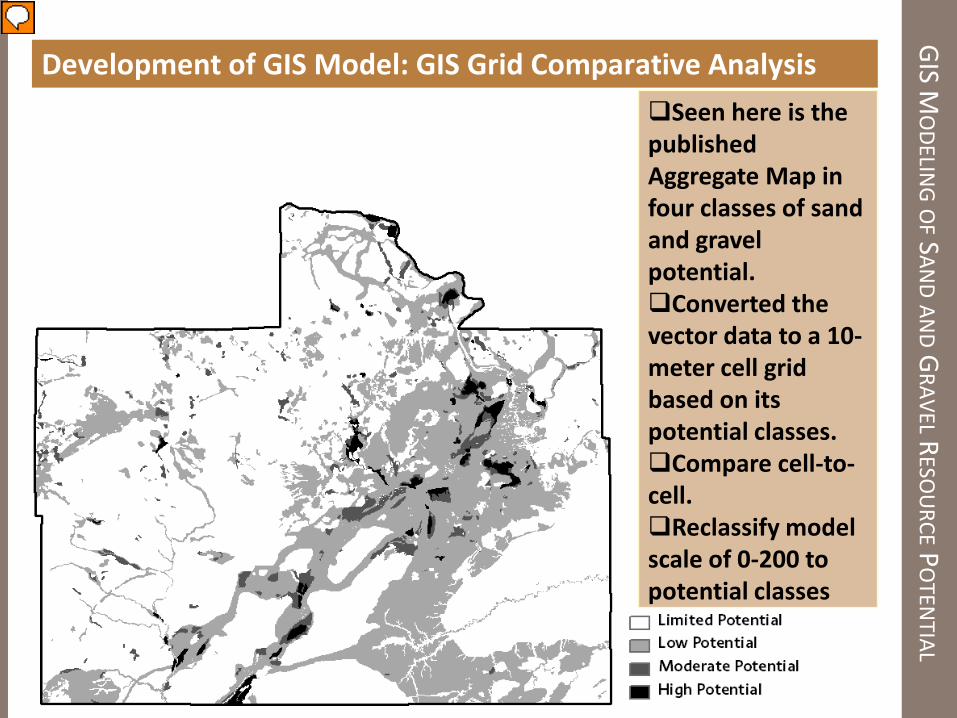
Development of GIS Model: GIS Grid Comparative Analysis Seen here is the published Aggregate Map in four classes of sand and gravel potential. Converted the vector data to a 10-meter cell grid based on its potential classes. Compare cell-to-cell. Reclassify model scale of 0-200 to potential classes

Presenter

Presentation Notes

Click Click Click Click

GIS MO

DELING O

F SAND AN

D GRAVEL R

ESOU

RCE PO

TENTIAL

Development of GIS Model: GIS Grid Comparative Analysis In order to

reclassify the modeled values (0-200) to the needed four classes the ArcGIS Zonal Statistics tool was applied. Zonal statistics was able to determine the mean, median, and Standard deviation for the final model cells that fell into one of the four potential classes from the completed map. This is show in the table to the left.

Presenter

Presentation Notes

Click, Click, Click This analysis was then used to reclassify the values from 0-200 to 1-4. (click)

GIS MO

DELING O

F SAND AN

D GRAVEL R

ESOU

RCE PO

TENTIAL

Development of GIS Model: GIS Grid Comparative Analysis The range of values

selected for reclassification can be seen in the table at the bottom left. Zonal statistics was applied on the new reclassed modeled grid (values 1-4) The results are shown in the table below.

GIS MO

DELING O

F SAND AN

D GRAVEL R

ESOU

RCE PO

TENTIAL

Development of GIS Model: GIS Grid Comparative Analysis Note the field

percent total area and visually compare it to the published aggregate data in the table below. See similarities? It is very important to note how much area is taken up in the project area by nonsignificant potential (limited and low). 90-95%

Presenter

Presentation Notes

Click

GIS MO

DELING O

F SAND AN

D GRAVEL R

ESOU

RCE PO

TENTIAL

Development of GIS Model: GIS Grid Comparative Analysis In order to do a cell-by-cell comparison of the model vs. the published map, ArcGIS raster calculator was applied The calculator was able to deliver a count of where the final model cell was equal to the aggregate mapping cell at the same location. Two tables were created to display the results

GIS MO

DELING O

F SAND AN

D GRAVEL R

ESOU

RCE PO

TENTIAL

Development of GIS Model: Finally the visual comparison…

Aggregate Program

Presenter

Presentation Notes

The project

GIS MO

DELING O

F SAND AN

D GRAVEL R

ESOU

RCE PO

TENTIAL

Development of GIS Model: Finally the visual comparison…

Sand & Gravel Model

Presenter

Presentation Notes

The project

GIS MO

DELING O

F SAND AN

D GRAVEL R

ESOU

RCE PO

TENTIAL

Development of GIS Model: Was it worth it?

The model did well, however it can not replace the level of detail in digital data creation (attributes), confirmation drilling, and the geologist expert interpretation when digitizing landforms using air photos. The model can however, and has been, a tool to apply before the geologist begins a new project. In a sense the model is doing a lot of the interpretive geologic leg work prior to beginning a project. The model can be useful in the field and during drilling to focus the geologist field work and time to significant sand and gravel rich areas. Lastly the project geologist has a modeled grid to assist with or confirm their interpretations when delineating sand and gravel potential.

Presenter

Presentation Notes

The project

GIS MO

DELING O

F SAND AN

D GRAVEL R

ESOU

RCE PO

TENTIAL

Development of GIS Model: Thank You

QUESTIONS Thanks to the SMUMN GIS Staff for all their help Thanks to Hannah Friedrich, the aggregate geologist, who help me rank and weight the modeled grids.

development and assessment of a gis based model to

Documents