development and application of soft computing and data mining … · 2013. 8. 21. · mas...
TRANSCRIPT

Andrés Sanz García
Development and application of soft computing and datamining techniques in hot dip galvanising
Francisco Javier Martínez de Pisón Ascacíbar
Ingeniería Mecánica
2012-2013
Título
Autor/es
Director/es
Facultad
Titulación
Departamento
TESIS DOCTORAL
Curso Académico

© El autor© Universidad de La Rioja, Servicio de Publicaciones, 2013
publicaciones.unirioja.esE-mail: [email protected]
ISBN 978-84-695-7622-9
Development and application of soft computing and data mining techniques inhot dip galvanising, tesis doctoral
de Andrés Sanz García, dirigida por Francisco Javier Martínez de Pisón Ascacíbar (publicada por la Universidad de La Rioja), se difunde bajo una Licencia
Creative Commons Reconocimiento-NoComercial-SinObraDerivada 3.0 Unported. Permisos que vayan más allá de lo cubierto por esta licencia pueden solicitarse a los
titulares del copyright.

Development and Application of Soft Computing and
Data Mining Techniques in Hot Dip Galvanising
Andrés Sanz García
A thesis submitted in
fulfilment of the requirement for the award of the
Degree of Doctor of Engineering
DEPARTMENT OF MECHANICAL ENGINEERING
UNIVERSITY OF LA RIOJA
JANUARY 2013


I hereby declare that this thesis entitled “Development and application of Soft
Computing and Data Mining techniques in Hot Dip Galvanising” is the result of
my own research except as cited in the references. This thesis has not been
accepted for any degree and is not concurrently submitted in candidature of any
other degree.
Signature :
Student : Andrés Sanz García
Date : December 2012
Supervisor : Dr. Francisco Javier Martínez de Pisón Ascacibar
Co-Supervisor:
iii

For my beloved mother
iv

Acknowledgments
I would like to start these acknowledgements saying ‘thank you’ to my mother
Carmen for her love and the possibilities she has created for me, and my brother
Iñigo who has always helped me. I would also like to thank those who over
the years have given me their friendship but they are too numerous to mention
all of them here. Other members of my family, many friends and particularly
Almudena, whose constant encouragement and great patience have been there
through all the difficult times.
I wish to express my gratitude to the Universidad de La Rioja. Especially
I would like to thank the partnership and support of the members of the EDMANS
research group and Department of Mechanical Engineering. Thanks to supervisor
Dr. Martínez de Pisón who has taught me a lot not only on this research topic
but life in general. I owe special thanks to Dr. Hollmén and the rest of the
School of Science from Aalto University, for hosting my two research visits and
solving any doubts. Last, I am deeply indebted with Dr. Escobedo of Helsinki
University. Thank you very much for your patience and constructive comments
on the thesis.
Finally, I also thank the Autonomous Government of La Rioja for support
through its 3rd R&D&i Plan within Project FOMENTA 2010/13, the University
of La Rioja for the support with both grants ATUR11/64 and ATUR12/45.
Andrés Sanz García, Logroño
v

vi Acknowledgments
vi

Abstract
In a world in which markets are more globalised and continuously evolving, com-
panies need new tools to help them enhance their flexibility to maintain their
competitiveness. To this end, a key strategy is the discovery of useful knowledge
through the information gathered from businesses and production processes. In
recent decades, many companies that are aware of this necessity have increased
their investments for improving both data storage capacity and information man-
agement. Currently, the huge volume of information stored by companies and its
high complexity render traditional methods of data processing useless, posing
serious problems for industry. However, the use of accurate tools to extract the
information hidden inside industrial databases, and then transform it into expli-
cit knowledge, is still under development. The creation and application of such
methodologies will make the key points of industrial processes more flexible, and
thereby fulfil the needs of global markets.
With the aim of solving this problem, new computer-based methodologies
derived from data mining are being developed. By using these methods, research-
ers are seeking to obtain non-trivial hidden knowledge from historical records of
industrial processes. For this reason, data mining has now become a crucial dis-
cipline for performing automatic searches inside historical industrial databases,
contributing to industrial development and advancement. Data mining involves
several techniques from different disciplines, such as statistics, machine learning
and artificial intelligence, among others.
This thesis focuses on the use of data mining techniques to develop help-
ful semiautomatic methods for tuning industrial production lines. The goal is
to increase flexibility in industrial processes in response to the need to meet
new consumer expectations and continue being competitive. The methodologies
developed have been used to study and improve a continuous galvanising line.
vii

viii Abstract
Bearing in mind its complexity, our aim is to explore the opportunities that data
mining techniques can offer for improving this industrial process.
The techniques used during the writing of this thesis are classified into
two categories: descriptive, for association rule mining; and predictive, for mod-
elling based on soft computing. Soft computing is defined as “obtaining solutions
by the use of intelligence, common sense or approximation by emulating human
behaviour”.
The goal of the first part of this thesis is to seek novel non-trivial know-
ledge in the form of patterns to help explain failures in production lines. To this
end, an overall methodology that integrates both data management and associ-
ation rule mining is proposed. Our aim is to capture those frequent events that
coincide when there is a failure in the industrial process studied.
The second part focuses on improving the modelling of non-linear dy-
namic systems using historical information from industrial processes. In this
case, the strategy is based on combining different soft computing techniques.
The techniques developed are designed to improve the estimation of temperature
set points for an annealing furnace on the galvanising line studied.
The contributions presented in this doctoral thesis provide evidence of
the huge potential that data mining has for obtaining useful, comprehensible
knowledge from industrial processes.
viii

Resumen
En un mundo donde los mercados son cada día más globales y cambiantes, la
industria necesita del apoyo de nuevas herramientas para mejorar su flexibilidad
operacional y continuar manteniendo altos niveles de competitividad. Una estra-
tegia clave para esta mejora es la búsqueda de conocimiento útil a partir de la
información procedente de sus procesos productivos y empresariales. En las úl-
timas décadas, las empresas han realizado importantes inversiones para mejorar
el almacenamiento y procesado de dicha información. Sin embargo, aún es muy
incipiente en la industria, la implementación de herramientas que extraigan el
conocimiento implícito subyacente en su información almacenada para transfor-
marlo en explícito, permitiendo así flexibilizar sus procesos.
Debido al volumen de información almacenada y su elevada complejidad,
los métodos tradicionales de procesamiento de datos no pueden ser empleados
hoy en día. Esto representa un grave problema para la industria. Por ello, se
están desarrollando metodologías basadas en el uso de computadoras para obtener
conocimiento útil a partir de datos históricos de procesos industriales. La minería
de datos se ha convertido en una disciplina crucial para realizar esta búsqueda de
forma automática en grandes bases de datos. Esta disciplina se nutre de numerosas
técnicas procedentes de otras tales como la estadística, el aprendizaje automático
y la inteligencia artificial entre otras.
Con la realización de esta tesis doctoral se pretende desarrollar metodolo-
gías basadas en minería de datos que ayuden al ajuste de las líneas de producción
industrial. El objetivo es conseguir mayor flexibilidad y eficiencia en la fabrica-
ción de nuevos productos. Para demostrar su aplicación práctica, las metodologías
propuestas han sido empleadas en el estudio y mejora de una línea de galvanizado
continuo por inmersión en caliente de bobinas de acero. La dimensión y comple-
jidad de la misma pretenden poner de manifiesto las oportunidades que ofrece la
ix

x Resumen
minería de datos en la mejora de este proceso industrial.
Las técnicas empleadas en la realización de esta tesis se engloban bajo
dos categorías diferentes: descriptivas para la extracción de reglas de asociación,
y predictivas, basadas en Soft Computing, con el objetivo de modelar sistemas.
Soft Computing se puede definir como “la obtención de soluciones mediante el
uso de la inteligencia, el sentido común o la aproximación por imitación a los
seres humanos”.
El objetivo de la primera parte de esta tesis doctoral ha consistido en
la extracción de conocimiento útil y no trivial en forma de patrones que permi-
tan explicar fallos frecuentes en líneas de producción. Para ello, se propone una
metodología global que integra tratamiento de datos y minería de reglas de aso-
ciación para mostrar eventos que aparecen con alto grado de coocurrencia cuando
se producen fallos en el proceso.
La segunda parte se ha centrado en la mejora del modelado de siste-
mas dinámicos no lineales a partir de datos históricos del proceso industrial. En
este caso, se desarrollaron dos metodologías basadas en la combinación de dis-
tintas técnicas de Soft Computing. Estas metodologías permitieron mejorar la
estimación de las temperaturas de consigna del horno de recocido de la línea de
galvanizado estudiada.
Las contribuciones presentadas en esta tesis doctoral demuestran el enor-
me potencial de la minería de datos a la hora de proporcionar conocimiento útil
y comprensible a partir de datos históricos de procesos industriales.
x
Contents
Declaration iii
Dedication iv
Acknowledgments v
Abstract vii
Resumen ix
List of Figures xiii
List of Tables xiv
List of Appendices xv
List of Symbols and Nomenclature xx
1 Introduction 1
1.1 Continuous hot dip galvanising and annealing furnace 6
1.2 Problem statement 9
1.3 Scope and Objectives 10
1.4 Contributions presented in the thesis 12
1.4.1 Publications of the thesis 14
1.4.2 Thematic unit 14
1.5 Thesis outline 15
2 Related Work 17
2.1 Association rules mining in industrial time series 18
2.2 Non-linear modelling of industrial process 20
3 PUBLICATION I 25
xi

xii Contents
4 PUBLICATION II 43
5 PUBLICATION III 57
6 Results 69
6.1 Results in Publication I 70
6.2 Results in Publication II 72
6.3 Results in Publication III 75
7 Discussion 79
8 Conclusions 91
Bibliography 93
xii
List of Figures
1.1 Basic scheme of actual framework of companies and DM tools 2
1.2 Basic procedure for developing models (from Norgaard et al., 2003) 4
1.3 Simplified scheme of a continuous hot dip galvanising line 7
1.4 Thermal galvanising cycle in CHDGL (from Chen et al., 2008) 8
1.5 Thermal annealing cycle in a CAF (from Ueda et al., 1991) 9
B.1 Evolution of attribute selection for all inputs in THC3 models 118
B.2 Evolution of attribute selection for all inputs in THC5 models 119
B.3 Complete range of RMSE via aggregation coefficients W : THC1 120
B.4 Complete range of RMSE via aggregation coefficients W : THC3 120
B.5 Complete range of RMSE via aggregation coefficients W : THC5 121
xiii

List of Tables
A.1 Rules extracted from the CHDGL database (part 1 of 3) 114
A.2 Rules extracted from the CHDGL database (part 2 of 3) 115
A.3 Rules extracted from the CHDGL database (part 3 of 3) 116
xiv

List of Appendices
A Supplementary material for Publication I 113
B Supplementary material for Publication II 117
xv

xvi List of Appendices
xvi

List of Symbols and Nomenclature
χ mutation factor
η learning rate of back propagation alg.
µ weighting coef. of complexity term
Al, Cu, Ni, Cr, Nb chemical composition of steel (in percentage of weight)
C, Mn, Si, S, P chemical composition of steel (in percentage of weight)
Conseq consequent
CV coefficient of variation
E event sequence dataset
G total number of generations
H number of neurons in hidden layer
I num. of best indiv. for early stopping
J fitness function
M momentum of back propagation alg.
MAE mean absolute error
ME mean - superscript -
N total num. of simulations for models
P population size
q binary array for feature selection
xvii
xviii List of Appendices
R compression rate
R2 Pearson´s correlation coefficient
RelConfidenceWinRule relative confidence within a time window
RelSupportWinRule relative support within a time window
RMSE root mean squared error
SD standard deviation - superscript -
T transactional episode database
t comp. cost for training models
Tg period of stability
THC1 Zone 1 Set Point Temperature (ºC)
THC3 Zone 3 Set Point Temperature (ºC)
THC5 Zone 5 Set Point Temperature (ºC)
ThickCoil strip thickness at the annealing furnace inlet (mm)
T imeLag window time-tag (ut)
TMP P 1 strip temperature at the heating zone inlet (ºC)
TMP P 2 strip temperature at the heating zone outlet (ºC)
TMP P 2CNG strip temperature at the heating zone outlet (ºC)
V, T i, B, N chemical composition of steel (in percentage of weight)
V elMed strip velocity inside the annealing furnace (m/min−1)
W complexity term
WidthCoil strip width at the annealing furnace inlet (mm)
WinW window width (ut)
xe elitism percentage
xg fraction for adjusting penalty function
xCI proportion of confidence interval
xval proportion of validation data
xviii
Devel. and Applic. of SC and DM Techniques in Hot Dip Galvanising xix
AI artificial intelligence
ANN artificial neural network
AR additive regression
ARM association rule mining
BG bootstrap aggregating (bagging)
CAF continuous annealing furnace
CHDGL continuous hot dip galvanising line
DB database
DG dagging
DM data mining
EC evolutionary computing
EM ensemble method
ESC early stopping criterion
FS feature selection
GA genetic algorithm
GA–NN genetic algorithm guided neural network
KDD knowledge discovery in databases
KM knowledge management
k-NN k-nearest neighbour
LMSQ least median squared linear regression
LR linear regression
MLP multilayer perceptron
xix

xx List of Appendices
M5P Quinlan´s improved M5 algorithm
RBFN radial basis function network
SC soft computing
SVM support vector machine
PCA principal component analysis
TDB transactional database
TDM temporal data mining
TS times series
TSKR time series knowledge representation
UT unification-based temporal
xx
Chapter 1
Introduction
The maximisation of profits from existing plants is a constant in steel industry due
to the large investments and long-term payback times of new plants. Steel com-
panies constantly need to cut costs while increasing productivity, with no reduc-
tion in product quality (Okereke & McDaniels, 2012; Madureira, 2012). In such a
context, an organisation´s goal is to select optimal strategies to ensure the max-
imisation of profits in all circumstances (Hoppe, 2002; Moffat, 2009; Cheng et al.,
2009). However, the selection is not so easy matter and has started to become
a serious problem in today´s globalised and ever-changing markets (OEC, 2006;
Int, 2010).
One way of overcoming this problem is to develop new tools that help
steel companies to gain deeper insights into their operations (Malerba, 2007;
GmbH, 2009; Lee et al., 2009). A better understanding of the “underlying prin-
ciples” of their processes would allow companies to increase their intellectual cap-
ital and make them more competitive (Harvey & Lusch, 1999; Femminella et al.,
1999; Lee et al., 2012; Lengnick-Hall & Griffith, 2011).
In recent decades, companies have started to become aware of this need to
increase their intellectual capital, making large investments in data acquisition,
data storage and information processing systems (Erickson & Rothberg, 2009;
Lücking, 2011). As data-capture and data-storage technologies are comparatively
low cost, a common characteristic of modern factories is now exponential growth
in size of their databases (DBs), which contain large volumes of data from their
processes (see Figure 1.1).
1

2 Chapter 1. Introduction
Figure 1.1: Basic scheme of actual framework of companies and DM tools
This huge amount of data theoretically contains hidden knowledge that
could help companies to gain competitive advantages in current markets by ex-
plaining multiple failures in their processes (Alfonso-Cendón et al., 2010), es-
timating product properties on-line (Ordieres et al., 2004), identifying relevant
features that compromise product quality (Agarwal & Shivpuri, 2012), helping
to predict process set points (Jelali, 2006), and so on. Indeed, the data stored
seems to contain an incredible potential that has been widely investigated by
many researchers (Hodgson, 1996; Kusiak & Zuziak, 2002; Bloch & Denoeux,
2003; Li & Dong, 2011), although it is agreed that raw information is rarely of
direct benefit (Harding et al., 2006; Köksal et al., 2011).
Companies have traditionally used manual procedures performed by pro-
cess analysts to handle their DBs and prepare reports, extract conclusions, dis-
cover rules or undertake other tasks related to knowledge management (KM).
There is now more evidence than ever that processing data collected from com-
pany processes using only traditional methods is wholly unfeasible because of
their size. Consequently, this has led to the need to discard manual methodolo-
gies in favour of automatic tools (Schiefer et al., 1999; Ordieres et al., 2004).
Analysts and experts also stress that the scale of the problem will stead-
ily an increasingly outpace human capacities. The avalanche of information
will render it more difficult to extract useful conclusions underpinning today´s
decision-making procedures (Kantardzic, 2011). This phenomenon has triggered
corporate interest in developing new automatic computer-based methodologies
that efficiently deal with large DBs to extract useful knowledge. Questions re-
2
Devel. and Applic. of SC and DM Techniques in Hot Dip Galvanising 3
garding the most suitable techniques for discovering hidden knowledge are often
solved by focusing attention on existing facilities (Aldrich, 2002).
A promising approach to this problem, and one that exploits the huge
quantity of historical records stored in DBs today, is the application of tech-
niques of knowledge discovery in databases (KDD) (Maimon & Rokach, 2008).
KDD is concerned with the task of extracting non-trivial useful knowledge from
large volumes of data (Mannila, 1997). This multi-disciplinary field is frequently
described as “mining information from the input data” and in fact, the essential
step in KDD is called data mining (DM). The two fields are very closely related
in terms of methodology and terminology (Mitra et al., 2002).
The actual DM task is defined by Hand et al. (2001). DM can automat-
ically identify interesting patterns in large volumes of data and try to extract
knowledge from them, transforming the original data into an understandable
structure of information for further use (Chapman et al., 2000). In recent years,
this field has started to be widely used in many disciplines of engineering and
science, such as electrical power engineering, bioinformatics, medicine and geo-
graphy.
In practise, DM involves the application of low-level algorithms to reveal
hidden information in large volumes of data (Miller & Han, 2001; Han & Kamber,
2006). Nevertheless, the implementation of the DM process is definitely not an
easy task, since most of the DM techniques are independent and their combination
does not often lead to better solutions. As Yang & Wu (2006) indicate, the
potential of these techniques is still unknown and we are far from answering such
questions as wether we can discover Newton´s laws from observing the movements
of objects.
There is a fair amount of evidence (Cox et al., 2002; González-Marcos,
2007; Martínez-De-Pisón, 2003; Maimon & Rokach, 2008) showing that DM is a
promising approach to which the steel industry is turning its attention. Many
authors posit (Marakas, 1998; Giudici & Figini, 2009) that DM has unique prop-
erties that may enhance competitive advantages if developed for such industrial
domains. However, although there have been several encouraging results, the
real world is often far from ideal, and DM is currently an open research topic
(Köksal et al., 2011). Without developing efficient methodologies, the DM tech-
niques themselves and the effort required to collect the data from a real prob-
lem do not provide commercial advantages to companies in industrial domains
(He et al., 2009).
3

4 Chapter 1. Introduction
Figure 1.2: Basic procedure for developing models (from Norgaard et al., 2003)
On one hand, the massive times series (TS) captured from industrial
environments are generally contaminated by noise. The conditions at industrial
plants create many inaccurate and spurious data (outliers) due to electromagnetic
interferences, phantom loads, power-line surges from plant machinery, etc. Hand-
ling noisy data and simultaneously gathering meaningful information from them
render the DM process more complex. Although major advances have been re-
ported in pre-processing of TS, tasks such as the automatic elimination of outliers
or noise filtering are still extremely difficult (Dürr et al., 2005).
On the other hand, most of industrial TS must be considered as non-static
and unbalanced data that are far from being independently and identically distrib-
uted (iid). This is because historical records from processes are usually composed
of many variables of different types with multiple non-linear relations.
New automatic or semi-automatic methodologies based on DM should
deal with all the factors described above. With minimal human assistance, they
have to solve the industrial problem for which they were created. These issues
mean their development and subsequent implementation are extremely challen-
ging. Additionally, our aim here was to obtain a reliable evaluation. We thus
4

Devel. and Applic. of SC and DM Techniques in Hot Dip Galvanising 5
extended our list of goals to include a final task of applying the methodology to
a real industrial case. The evaluation consisted of a list of criteria for assessing
how our methodology performed in real situation (see Figure 1.2).
In order to evaluate the proposals, a list of process candidates of proven
significance within the steel industry was generated. The case study, details of
which are provided below, was finally selected from this list, taking into consid-
eration mainly its complexity, the availability of real data and the existence of
plant experts. Some phenomena in industrial processes are not so readily under-
standable. There are several specific cases in which explanations require complex
descriptive structures or non-linear predictive models. Moreover, the problem of
finding the latent structure of these phenomena is very challenging due to the
high-dimensional data collected.
This thesis focuses on the use of DM techniques to develop helpful semi-
automatic methods for tuning industrial production lines. Our goal is to increase
flexibility in industrial processes to fulfil new consumer expectations quickly in
order to continue being competitive. The methodologies developed have been
used to study and improve a continuous galvanising line.
A continuous hot dip galvanising line (CHDGL) is a clear example that
featuring all the problems and requisites that we seek to address in this thesis
(Bian et al., 2006; Mullinger & Jenkins, 2008). From an economic and strategic
point of view, CHDGL is a key process for steel companies. They have made
important investments to increase production by automating the entire process
and reducing the number of operations in which humans operators are involved.
The automation process has brought new problems and the situation is now
becoming more serious owing to a steady increase in the demand for cheaper
rolled flat steel products.
The need to produce high quality galvanised products without decreasing
line capacity has also created a need for additional improvements in the auto-
mation systems, such as more reliable on-line monitoring systems and accurate
models for predicting process set points (Zhong et al., 2002; Suarez et al., 2010),
for example.
Historically (Ueda et al., 1991), improvement in the monitoring and con-
trol system in CHDGLs has been based largely on mathematical models that have
usually been implemented instead of expensive plant trials (199, 1998; Tian et al.,
2000).
5

6 Chapter 1. Introduction
The initial motivation for this thesis is based mainly on the previous
work of Bloch et al. (1997), Schiefer et al. (1999), and Martínez-De-Pisón (2003).
These publications mark a change in the direction from mathematical approach,
developing new models to replace previous ones. From the very outset, the res-
ults of these initial papers began to reveal more accuracy and reliability than
traditional techniques (Ordieres et al., 2004, 2005; Pernía-Espinoza et al., 2005;
Li et al., 2006; Pal et al., 2006; González-Marcos, 2007), generating a research
field in which many improvements have been widely reported in different com-
ponents of CHDGL (Martínez-De-Pisón et al., 2006, 2010a).
Two recent papers (Martínez-De-Pisón et al., 2010b, 2011) that improve
the prediction of the temperature set points in a continuous annealing furnace
(CAF) and an additional work (Ordieres-Meré et al., 2010) predicting the prop-
erties of galvanised steel strip are considered as the basis for the work presented
in this thesis. Furthermore, following the good performance achieved with the
proposals made in those papers, there is still ample scope for improvement, espe-
cially in robustness, reliability and the capacity for generalisation in predicting
novel data. This has been shown in recent research into different approaches
such as evolutionary artificial neural networks (ANNs) (Yang et al., 2011), sup-
port vector machines (SVMs) (Liu et al., 2011) and ensemble methods (EMs)
(Pardo et al., 2010; Niu et al., 2011; Okun, 2011)
A further aim was to provide qualitative information about the CHDGL
(Choo et al., 2007). We thus developed new descriptive models as another of
our goals. Detecting and identifying the causes of frequent failures in CHDGLs
is essential to ensuring plant productivity and the product quality of galvanised
strip surface (Xu et al., 2009; Li et al., 2011a).
By drawung on the knowledge of plant engineers and using DM-based
approaches (Alfonso et al., 2012), several applications have been focused on this
specific problem (Gonzalez et al., 2006; Zhang et al., 2010). Through this altern-
ative approach, the research is closely related with other previous publications,
such as (Alfonso-Cendón et al., 2010; Posada, 2011; Ferreiro et al., 2011).
1.1 Continuous hot dip galvanising and annealing furnace
CHDGL is briefly described in this section because the experimental validation
of our methodologies lies in the historical records from a real galvanising line
6

Devel. and Applic. of SC and DM Techniques in Hot Dip Galvanising 7
located in northern Spain.
Figure 1.3: Simplified scheme of a continuous hot dip galvanising line
Galvanised steel is widely used due to its corrosion protection in many
applications, such us automotive body parts, electrical transmission and appliance
industry (Rentz & Schltmann, 1999). The process of galvanising steel products is
broken down according to its technology into continuous and discontinuous, but
continuous process is the only one used to coating steel coils and also the more
economical for mass output (González-Marcos, 2007).
Broadly speaking, the different continuous galvanising lines can be clas-
sified into the following three types: combined annealing and galvanising line, hot
dip galvanising line and hot strip continuous galvanising line (Ame, 2006). The
second type of line involves applying a zinc coating to steel products to protect
the steel from corrosion by immersing the preheated material in a bath consisting
primarily of molten zinc.
This thesis focuses on a continuous hot dip galvanising process for steel
coils. This technology has several advantages over others, such as relatively low
costs and high volume production (Martínez-De-Pisón, 2003). However, as men-
tioned earlier in Chapter 1, most of the research in this thesis is directly related
to the CAF on the CHDGL studied, which is the heart of the annealing process
(Pernía-Espinoza et al., 2005).
A CHDGL for steel coils contains mainly five separate sections that per-
form a particular treatment on the steel strip during the process (Figure 1.3):
1. Pre-heating area
2. Heating and holding area
7

8 Chapter 1. Introduction
3. Slow cooling area
4. Jet cooling area
5. Overaging area
The following paragraph describes the particular process that was selected as
case of study in this thesis. However, the description can be applied, with certain
minor modifications, to other industrial plants worldwide.
Figure 1.4: Thermal galvanising cycle in CHDGL (from Chen et al., 2008)
First, initial steel coils from the cold-rolling process need to be unwound,
welded together to form a continuous strip and cleaned, then fed into the an-
nealing furnace. Once the steel strip is inside the furnace, it runs through a
number of vertical loops to obtain pre-established temperatures according to an
annealing cycle. The steel strip subsequent passes through a molten zinc coating
bath followed by an air stream “wipe” that controls the thickness of the zinc
coating. Finally, the strip is treated by a series of auxiliary processes, forming a
coil shaped product.
The initial surface preparation of the base metal is critical for maintaining
the quality of the galvanised steel products. Nevertheless, three additional zones
also have to be controlled to ensure the uniformity of the zinc film in an immersion
process: the molten zinc bath, the CAF, and the air-cooling jet. Note that a more
detailed description of the galvanising line is provided in Vergara (1999).
The annealing treatment is applied to the steel strip to heat it and main-
8

Devel. and Applic. of SC and DM Techniques in Hot Dip Galvanising 9
Figure 1.5: Thermal annealing cycle in a CAF (from Ueda et al., 1991)
tain it at an appropriate temperature, followed by a cooling process at different
rates. In short, each cold rolled coil has to be subjected to a heat treatment to
improve its mechanical properties and the uniformity of the zinc coating (Tang,
1999). Figure 1.4 and Figure 1.5 show two examples of different profiles of an-
nealing cycles, a thermal cycle for steel samples in a CHDGL (Chen et al., 2008)
and strip temperature cycle in a CAF (Ueda et al., 1991), respectively.
The standard control of the CAF usually involves maintaining the strip
velocity within a pre-established range of values while managing the temperature
settings in each zone (Yoshitani & Hasegawa, 1998). Today, the efficient and
cost-effective operation of a CAF is unimaginable without integrated automation
systems. The introduction of improved automation systems or better furnace
regime controls allows the line speed and, consequently, its ouput to be increased.
Nevertheless, there is still a great problem when dealing with new coils made from
steel with a different chemical composition or with dimensions that have not
been previously mapped. CAF control systems face the same problems as other
continuous industrial processes in the steel industry, namely, very low flexibility.
1.2 Problem statement
Over the past twenty years, companies have invested to increase their output of
galvanised flat steel products to meet an increase in global demand. In addition,
today´s markets are rapidly evolving, so production lines have to be adjusted to
meet fresh consumer needs in the shortest period of time.
This situation has led galvanising companies to search for greater oper-
ational flexibility in production plants. They have started to develop new tools
9

10 Chapter 1. Introduction
to allow plant engineers to quickly adjust galvanising lines to new processing
conditions.
These tools may be composed of several elements that perform many
different tasks such as estimation, control, monitoring, classification, etc. In the
galvanising industry, the development of these components is a truly daunting
task due to the complexity and inherent nonlinearities of their underlying pro-
cesses. There exists a general consensus on the need for profound and accurate
knowledge on the galvanising process for performing this task.
This knowledge was traditionally found by conducting a number of in-
plant process trials, but this is inefficient due to the high costs involved. The
most widely used alternative is to use mathematical methods considering the
physical properties and mechanics of the process. However, this approach involves
great difficulties for swiftly adjusting the component parameters to new product
specifications, often requiring high computation time.
The problem addressed in this thesis is the difficulty in making estimates
and multiple adjustments for tuning a galvanising line when dealing with new
products. One possible approach is to extract the knowledge from the large
volumes of data usually captured from the CHDGLs. Most galvanising companies
can afford real-time data warehouses or large DBs, but they are unable to take
advantage of that “stored knowledge” to save costs.
This challenging problem requires the development of new efficient DM-
based methodologies capable of handling large DBs while generating useful know-
ledge that helps plant engineers to reduce the time required for performing many
operational tasks such as estimating optimal set points, explaining failures in the
line, scheduling production operations, identifying and classifying product defects
during the zinc coating, and so on.
1.3 Scope and Objectives
The scale of data analysis, rule generation and even inferencing in industrial DBs
have outrun human capacities. Analysts and plant experts are constantly trying
to implement new computer-based methodologies that could be profitably used
to extract “process knowledge”.
10

Devel. and Applic. of SC and DM Techniques in Hot Dip Galvanising 11
As mentioned above, steel industries need to enhance the flexibility of
their key processes to continue being competitive; an in-depth study of their
continuous production lines through DM can be extremely useful for tuning the
lines´ set parameters, as well as for identifying frequent failures in them.
How to address this need in the galvanising industry by using DM tech-
niques and predictive SC-based modelling is the main scope of this thesis, which
has the following five research objectives:
1. specify new semi-automatic methodologies based on DM and SC to obtain
knowledge for helping to improve galvanising lines;
2. apply the methodologies proposed in a CHDGL for steel coils, and more
specifically to its CAF;
3. evaluate the performance of the methodologies. The proposals will be val-
idated using the data from a CHDGL, whereupon the results detained will
be evaluated to decide whether the models developed reflect significant im-
provements;
4. report a convincing discussion about the knowledge discovered in any of its
possible forms, such as rules or overall parsimonious prediction models, and
create new opportunities for future developments;
5. hand the knowledge obtained over to operators and plant engineers for
its implementation in galvanising plants. This knowledge may be used
to automate the tuning of galvanising process that was previously being
operated manually.
It should be noted that the validation of the proposals has focused solely on ex-
tracting knowledge related to the quality of continuously galvanised coils. How-
ever, it is worth mentioning that methodologies of this kind can be used not only
for extracting knowledge from this particular industrial process but also extra-
polated, with the same potential success, to other fields such as the environment,
energy, business, marketing, etc.
11

12 Chapter 1. Introduction
1.4 Contributions presented in the thesis
This thesis considers three scientific contributions reported in the following pub-
lications referred to by Roman numerals:
Publication I (Martínez-de Pisón et al., 2012). An experience is presented
based on the use of association rules from multiple TS captured from
a galvanising process, where the main goal is to seek useful knowledge
for explaining failures in this process.
An overall methodology is proposed for obtaining the association
rules, which represent relations repeated between different pre-defined
episodes in multiple TS.
Each episode corresponds to a significant event in the TS, and it is
defined within a time window and with a time lag. The initial steps
of the proposed methodology involve an iterative, interactive process
that involves the use of several pre-processing and segmentation tech-
niques to obtain the significant events in each TS. A search is then
made according to a pre-established time window, a time lag, and a
pre-set consequent for finding sequences of episodes that are repeated
in various TS; lastly, the rules can be extracted for those frequent
episodes, i.e. episodes that have a large number of hits.
In our case, this methodology has been applied and validated by ex-
tensive experiments using a historical database of 150 variables from
a galvanising process for steel coils.
Experiments were designed by Martínez-de-Pisón and all of them were
jointly conducted with the auhtos. The author wrote most of the art-
icle and Martinez-de-Pisón wrote the other parts of the article.
Publication II (Sanz-García et al., 2012). A methodology is presented for
creating parsimonious models to predict set points in production lines.
The models generated have lower prediction errors, higher generalisa-
tion capacity and less complexity than those generated by a standard
method.
The main component of the proposal is a wrapper scheme that in-
cludes a multilayer perceptron (MLP) neural network. The number
of neurons in the unique hidden layer of the MLP, the inputs selec-
ted and the training parameters are optimised to record the fewest
errors. The article proposes genetic algorithms (GAs), whereby the
wrapper-based scheme is optimised. The optimisation process in-
12

Devel. and Applic. of SC and DM Techniques in Hot Dip Galvanising 13
cludes two fundamental components: a dynamic penalty function to
control model complexity and an early stopping criterion (ESC) for
interrupting the optimisation phase.
Using the data obtained from the same process as in Publication I,
we performed an evaluation comparing our methodology and others
previously proposed.
The results show the advantages of our proposal for developing better
parsimonious models for predicting temperature set points in indus-
trial processes, and also highlight the potential proposal’s range of
applicability.
Martínez-de-Pisón provided insight into the theory and helped con-
siderably in the way toward a workable implementation. The author
implemented the mxethodology and wrote the article. Furthermore,
the author was responsible for planning, conducting, and reporting
the experiments.
Publication III (Sanz-García et al., 2013). This paper represents the next
step after the work started in Publication II.
Due to the global, evolving nature of the galvanising industry, there
is an increasing need to maintain the high quality of products while
working with continual changes in the production cycle.
With the aim of achieving better overall models for predicting set
points on the CAF, we explore the possibilities of EMs to increase
the scope for generalisation and reduce computation costs and the
expertise required during training. Three prediction models based on
EMs, namely additive regression (AR), bagging (BG) and dagging
(DG), are applied to the DB from the same CHDGL used in previous
publications. We have developed a comparative evaluation to demon-
strate the capacity of proposed EMs to create overall models from
industrial databases.
The resulting models perform better in terms of prediction and gener-
alisation capacity without loosing their parsimony, with a significant
decrease in the difficulty and cost of setting up the models.
The method was developed by the author. The author designed the
experiments, conducted all of them, and wrote the article.
13

14 Chapter 1. Introduction
1.4.1 Publications of the thesis
The present thesis consists of an brief introductory part and the following three
peer-reviewed publications in two journals listed in the Journal Citation Re-
ports®:
1. Martínez-de-Pisón, F., Sanz, A., Martínez-de-Pisón, E., Jiménez, E. &
Conti, D. (2012). Mining association rules from time series to explain fail-
ures in a hot-dip galvanising steel line, Computers & Industrial Engineering
63(1), 22-36
2. Sanz-García, A. and Fernández-Ceniceros, J. and Fernández-Martínez, R.
& Martínez-de-Pisón, F. J. (2012). Methodology based on genetic optim-
isation to develop overall parsimonious models for predicting temperature
settings on an annealing furnace, Ironmaking & Steelmaking, available on
line. DOI 10.1179/1743281212Y.0000000094
3. Sanz-García, A. and Antoñanzas-Torres, A. and Fernández-Ceniceros,
J. & Martínez-de-Pisón, F. J. (2012). Overall models based on ensemble
methods for predicting continuous annealing furnace temperature settings,
Ironmaking & Steelmaking. DOI 10.1179/1743281213Y.0000000104. Avail-
able on line
1.4.2 Thematic unit
The framework of three publications informing this thesis involves two main fields:
data mining and the galvanising process.
• The first publication (Martínez-de Pisón et al., 2012) focuses on the devel-
opment and validation of a methodology based on DM for discovering useful
knowledge. Specifically, an application based on ARM using a time window
and a time lag is proposed to find patterns in TS from an industrial pro-
cess. The procedure is validated with data collected from a real CHDGL,
and it is concluded that the methodology has the capability to extract novel
relations between several products and process features.
• The second (Sanz-García et al., 2012) and third (Sanz-García et al., 2013)
publications share the implementation of overall parsimonious models for
predicting the temperature set points of a CAF on a CHDGL. These contri-
14

Devel. and Applic. of SC and DM Techniques in Hot Dip Galvanising 15
butions provide two methodologies for faciliting the tasks of designing and
automatically selecting the best overall parsimonious model.
It is noteworthy that all three methodologies proposed were validated using the
historical data from the same CAF on a CHDGL.
1.5 Thesis outline
The document is divided into eight chapters and outlined as follows. Chapter 2
describes previous works on DM and predictive process modelling based on SC
for improving industrial processes, focusing especially on industrial applications.
Chapter 3, 4 and 5 correspond to the three peer-reviewed publications upon
which the thesis is based. Publication I corresponds to research on the field of
ARM and the extraction of useful knowledge to explain failures in continuous
production lines. Publications II and III both deal with the non-linear modelling
of an industrial process using data-driven methods. These publications focus on a
particular CHDGL for steel coils, and more specifically on its CAF. In Chapter 6,
the findings and results of the three papers are briefly summarised. The general
discussion of the thesis continues in Chapter 7, and the conclusions are finally
reported in Chapter 8.
15

16 Chapter 1. Introduction
16
Chapter 2
Related Work
This chapter covers recent advances in DM and SC techniques in ironmaking,
steelmaking and the manufacturing industry. Representative examples are selec-
ted from the numerous industrial applications in which these techniques have been
used for knowledge discovering and advanced modelling (Nisbet et al., 2009).
Nowadays, data are captured from industrial processes in many differ-
ent formats, such as text, numerical values, images, etc. However, according to
Hand et al. (2001), most of DM techniques focus on dealing with two classes of
data: qualitative and quantitative. The former is not so precisely defined and not
so specific as the latter. Descriptive techniques are used for working with qualit-
ative data. They are divided into several types depending on the task performed,
e.g., ARM is a descriptive technique for discovering relations between items based
on hidden patterns. In contrast, quantitative data can be approximated using
numerical values. Predictive methods can deal with quantitative data for infer-
ring models of dynamic systems from a series of measurements, taken from these
selfsame systems (Norgaard et al., 2003).
In recent years, there seems to have been exponential growth in DM-
based applications using both predictive and descriptive techniques in multiple
domains. Taken as a whole, both types are able to constitute highly elaborate
systems.
In 2009, Choudhary et al. reported a full review of several types of DM
techniques applied in manufacturing, emphasising on the type of DM function
to be performed on industrial data. However, some techniques employed in this
17

18 Chapter 2. Related Work
thesis, such as EMs and evolutionary computing (EC), were not included in their
review. Complementary information about EMs was provided by Rokach (2009)
together with further insight into the vast number of alternatives available. On
the other hand, Oduguwa et al. (2005) described in detail the status and trends
of EC, resolving a wide range of industrial problems.
Recently, Köksal et al. (2011) and Liao et al. (2012) have presented ad-
ditional up-to-date reviews describing many applications based on different DM
techniques for industry. Although the goals of DM-based applications in the
literature are very diverse, two activities are readily apparent: the increase in
end-product quality and the inference of non-linear systems for industrial lines.
Indeed, these are the main goals of the new methodologies developed in this
thesis. For this reason, this chapter is divided in two sectionsaccording to the
two types of data that the thesis tackles, i.e. ARM for extracting qualitative data
and non-parametric prediction modelling for predicting quantitative data .
2.1 Association rules mining in industrial time series
ARM in TS has generated a considerable interest in many domains in recent
years (Core & Goethals, 2010). Seminal works by Das et al. (1997, 1998) have
highlighted the capability that these techniques have for discovering patterns in
multivariate TS, in contrast to traditional analyses that focus largely on global
models. For instance, in order to enhance quality control in industry, a grow-
ing body of literature has examined the potential of ARM for extracting the
hidden knowledge within the TS from their industrial processes (Köksal et al.,
2011). Knowledge can be represented as a list of simple rules that would be help-
ful in decision-making for adopting measures to avoid drops in product quality
(Triantaphyllou et al., 2002; Ferreiro et al., 2011).
The basic idea of ARM involves finding frequently-repeated interrelations
among multiple TS, and depicting them in a manner that is readily understood
by an expert (Haji & Assadi, 2009).
One of the most widely known frameworks for carrying out this task is
temporal data mining (TDM). TDM is a set of techniques that extracts valuable
information associated with periods of time (Tak-Chung, 2011). According to
Abdel-Aal (2008), the interesting feature of TDM is that the presence of the
time attribute as a trigger allows more complex patterns to be obtained. These
18

Devel. and Applic. of SC and DM Techniques in Hot Dip Galvanising 19
patterns provide more scope for analysts in terms of understanding and utility, but
their proper interpretation usually incurs problems (Zhao & Bhowmick, 2003).
Another basic framework for extracting temporal patterns in TS is the
frequent episode discovery framework (Mannila et al., 1997). Generally speak-
ing of thinking, the point of departure for TDM is the work by Mannila et al.
(1997).
In 2000, Zaki (2000) showed how important it is to use constraints, es-
pecially time constraints, in the application of methods to obtain concise results
and useful information. Furthermore, in many TS, especially those related to
understanding industrial process failures (Shahbaz et al., 2006), the relationships
do not occur at the same instant in time, but with time lags. Therefore, the
search for events of interest in the antecedent should focus on a time window
located before a predefined type of event in the consequent. The development of
MOWCATL algorithm by Harms et al. (2002) was a significant advance in finding
minimal occurrences of episodes and relations between them, which occur within
the specified window width. More recently, Huang & Chang (2007) combined the
constraints during the discovery process, a time lag between the antecedent and
consequent of a discovered rule and relations with episodes from across multiple
sequences.
All these publications are closely related to the methodology proposed
for ARM in TS. However, in our case the concept of search windows is adopted
solely for the antecedent of the rules extracted. It can therefore be said that
the constraints on the consequent are increased, given that the desired event is
initially known and, what is more, the sole point of interest is the first instant at
which it occurs.
In 1994, Agrawal & Srikant defined the ARM in transactional databases
(TDBs) by using the APRIORI algorithm. However, the methodology proposed
in this thesis for extracting rules focuses primarily on framework proposed by
Mannila et al. (1997). Hence, mining “episodes” can be considered as our starting
point for obtaining temporal relations in a single TS with the aid of a sliding
(time) window. The combination of items in a sequence of events gives rise to an
episode with a specific order in time. This approach has been applied in many
domains, such as assembly lines in manufacturing plants (Laxman et al., 2004),
Wal-Mart sales DBs (Atallah et al., 2004), web navigation logs (Casas-Garriga,
2003), and so on.
19

20 Chapter 2. Related Work
Other strategies have proven to be even more powerful than the previous
ones expressing temporal concepts in interval sequences. In particular, the liter-
ature reports certain more complex approaches, such as pattern mining based on
Allen’s relations (Kam & Fu, 2000), rules expressed with unification-based tem-
poral (UT) grammar (Ultsch, 2004) and temporal rules with the hierarchical time
series knowledge representation (TSKR) (Mörchen & Ultsch, 2007). Their use is
sometimes not strictly necessary, as the depiction of information can become more
difficult to understand, making the pattern space complex for analysts.
The task of extracting minimal occurrences of episodes and relations
between them could be accomplished by means of the MINEPI algorithm de-
veloped by Mannila et al. (1997). Nevertheless, the ECLAT algorithm, proposed
by Zaki (2000), is usually used as the support for obtaining frequent item sets
in episode DBs. One reason is that ECLAT has proven to be very effective for
reducing computation time (Schmidt-Thieme, 2004). This does not mean that
ECLAT is the best choice. Indeed, many other algorithms capable of mining
for temporal rules in TSDB based on these three methods have been introduced
over the past decade. For example, ARMADA (Winarko & Roddick, 2007) and
CTMiner(Chen et al., 2010), among others. However, the use of ECLAT does
not reduce the degree of generalisation for providing an overall methodology.
The literature reports few applications of ARM for discovering previously
unknown rules that enable experts to adopt measures to avoid problems in real
industrial processes.
2.2 Non-linear modelling of industrial process
Soft computing attempts to find reasonably useful solutions to complex problems.
SC-based methods exploit the tolerance of uncertainty and imprecision to achieve
the greater robustness, manageability and lower computation cost of solutions
(Zadeh, 1994). The three popular constituents of SC are fuzzy sets, ANNs and
GAs (del Jesús et al., 2009).
In recent years, many authors have revealed a growing interest in SC
(Argyropoulos, 1990; Schlang et al., 1996, 1999). In 2001, Dote & Ovaska presen-
ted a broad review to eliminate the important gap between the theory and prac-
tice of these techniques. Choudhary et al. (2009) presented a full review of the
literature dealing with SC and DM applications in manufacturing domain. In
20

Devel. and Applic. of SC and DM Techniques in Hot Dip Galvanising 21
comparison to this lastest review, other papers focused more on steel processing;
so the following paragraphs deal explicitly with the industrial applications of SC
techniques.
In 2001, Schlang & Lang presented a number of applications of neural
computation for process control in steel processing. Takahashi (2001) described
various types of innovations based on Artificial Intelligence (AI) promoted in the
field of hot rolling process control. Tang et al. (2001) conducted a comparative
analysis of certain AI-based planning and scheduling systems for steel production.
These papers testify to the considerable amount of literature published on DM
and SC applications. However, of all the types of processes associated with indus-
trial domains, those for continuous galvanising and annealing were of particular
interest to this thesis.
As mentioned in Chapter 1, CHDGL always includes a CAF upstream of
the zinc bath to improve steel properties according to pre-established annealing
curves (see Figure 1.4 and Figure 1.5). The annealing treatment of steel coils
consists on accurately controlling heating and cooling temperature settings inside
a furnace while maintaining the strip velocity within a pre-established range of
values. The prediction of CAF temperature settings is an unresolved issue, and
several research papers have been published on the use of different approaches
for modelling the furnace. The ultimate goal is to enhance the online control of
the CAF (Prieto et al., 2005b,a).
Traditional approaches are based on determining temperatures empir-
ically by multiple process trials that create a set of tables (Martínez-De-Pisón,
2003). Today, this inefficient method has been discarded because of the high costs
associated with in-plant trials.
A well-known alternative is to develop mathematical models (model-
based approach) based on the thermodynamic properties of the furnace mater-
ials and the heat transfer mechanics inside the CAF (Jaluria, 1988; Townsend,
1988; 199, 1998; Sahay et al., 2004; Sahay & Kapur, 2007; Mehta & Sahay, 2009).
However, as Prieto et al. (2005b) contend, some furnace specifications and mater-
ial properties may change appreciably with different steel compositions and heat
treatment, and this may have a significantly bearing on mathematical models.
A further alternative is the development of models based on data (data-
based or data-driven approach). They may improve prediction capability be-
cause they consider not only the inherent non-linearities of the annealing process
21

22 Chapter 2. Related Work
but also the plant operators´ experience and historical data (Tenner et al., 2001;
Jones et al., 2005; de Medeiros et al., 2007).
Since 1998, in studies related to regression models, several authors have
reported on the use of historical data from steel processes (Yoshitani & Hasegawa,
1998; Schlang et al., 1999), and interest in such models has grown, especially in
those based on ANNs (Schlang & Lang, 2001), genetic algorithm guided neural
network (GA–NN) ensemble (Yang et al., 2011), fuzzy logic models (Hassan et al.,
2012) fuzzy ANNs (Li et al., 2011b), Bayesian models (Agarwal & Shivpuri, 2012),
Gaussian mixture models (Yang et al., 2012), among others.
Several applications can readily be found in the literature that apply
the fuzzy set theory in CHDGL for system control, quality management, etc.
Kuru & Kuru (2011) proposed a new galvannealing control system based on a
fuzzy inference system. This system contributed to a significant improvement
in the uniformity and quality of the coating layer running at the lower limit of
permissible coating values. More recently, Zhang et al. proposed a feed-forward
control method based on fuzzy adaptive models for the thickness control process
of galvanising coating (Zhang et al., 2012).
In galvanising, Lu & Markward (1997) reported significant improvements
using ANNs for coating control. Schiefer et al. (1999) presented a combination of
clustering and a radial basis function network (RBFN) for improving predictions
in the online control of galvannealing process. In 2005, Pernía-Espinoza et al.
(2005) reported the high performance of robust MLP for estimating the velocity
set point of coils inside the CAF using coil specifications and furnace temper-
atures. Along with this research, other promising papers have developed more
reliable models for predicting CAF temperature settings in CHDGL.
In an earlier paper, Martínez-De-Pisón et al. (2006) reported a method-
ology based on combining MLP networks and GAs. Their results showed that
correctly tuned MLPs can predict the optimal settings of a CAF control system.
Nevertheless, the task of finding the best MLP topology is still a challenging
problem. In 2010, Martínez-De-Pisón et al. provided support for the use of us-
ing MLPs with few hidden neurons instead of more complex networks to produce
models with less generalisation error. These models allowed them to predict CAF
temperature settings more accurately, in particular dealing with data not previ-
ously encountered. Based on previous papers, in 2010 Martínez-De-Pisón et al.
proposed an overall dynamic model for the strip temperature in the annealing
furnace.
22

Devel. and Applic. of SC and DM Techniques in Hot Dip Galvanising 23
The advent of GAs (Mitchell, 1998), which are widely used in many
industrial domains (Pal et al., 2006; Pettersson et al., 2009; Yang et al., 2011),
has made the task of finding optimal prediction models, especially those based
on ANNs, a more tractable problem. GAs are capable of optimising model set-
tings, striking a balance between accuracy and complexity on the one hand, and
resources invested in model development on the other. In 2010, Agarwal et al.
reported on work with evolutionary neural networks to estimate the expected
performance of a blast furnace with periodic variations in input parameters and
changes in operating conditions. Finally, in 2011, Martínez-De-Pisón et al. re-
ported a method based on GAs to find the optimal MLP, with the proposal then
being applied to a CAF. This paper enabled satisfactory heat treatments to be
given even in cases of sudden changes in strip specifications, such as welding two
coils that are totally different in terms of dimensions and chemical composition.
More research into modelling, system identification and control system
design is still needed to address the problem of dealing with new steel coils that
have not been previously mapped.
23

24 Chapter 2. Related Work
24
Chapter 3
PUBLICATION I
Martínez-de-Pisón, F., Sanz, A., Martínez-de-Pisón, E., Jiménez, E. & Conti,
D. (2012). Mining association rules from time series to explain failures in a
hot-dip galvanising steel line, Computers & Industrial Engineering 63(1), 22 -
36.DOI 10.1016/j.cie.2012.01.013.
The publisher and copyright holder corresponds to Elsevier Ltd. The online
version of this journal is the following URL:
• http://www.journals.elsevier.com/computers-and-industrial-engineering/
25

26 Chapter 3. PUBLICATION I
.......
26

Computers & Industrial Engineering 63 (2012) 22–36
Contents lists available at SciVerse ScienceDirect
Computers & Industrial Engineering
journal homepage: www.elsevier .com/ locate/caie
Mining association rules from time series to explain failuresin a hot-dip galvanizing steel line
Francisco Javier Martínez-de-Pisón a,⇑, Andrés Sanz a,1, Eduardo Martínez-de-Pisón a,2,Emilio Jiménez b,3, Dante Conti c,4
a EDMANS Group, Departamento de Ingeniería Mecánica, Edificio Departamental, Universidad de La Rioja, C/Luis de Ulloa 20, 26004 Logroño, La Rioja, Spain5
b IDG Group, Departamento de Ingeniería Mecánica, Edificio Departamental, Universidad de La Rioja, C/Luis de Ulloa 20, 26004 Logroño, La Rioja, Spainc Universidad de Los Andes, Mérida, Venezuela
a r t i c l e i n f o
Article history:Received 27 February 2010Received in revised form 16 January 2012Accepted 18 January 2012Available online 26 January 2012
Keywords:Cause failuresAssociation rulesKnowledge discoveryMultiple time seriesContinuous hot-dip galvanized line
0360-8352/$ - see front matter � 2012 Elsevier Ltd. Adoi:10.1016/j.cie.2012.01.013
⇑ Corresponding author. Permanent address: C/LuisEdificio Departamental, Universidad de La Rioja, Logr941 299 232; fax: +34 941 299 794.
E-mail addresses: [email protected] (F.J. Martunirioja.es (A. Sanz), [email protected]@unirioja.es (E. Jiménez), [email protected]
1 Permanent address: C/Luis de Ulloa, 20, DespachoUniversidad de La Rioja, Logroño, La Rioja, Spain. Tel.: +299 794.
2 Permanent address: C/Luis de Ulloa, 20, DespachoUniversidad de La Rioja, Logroño, La Rioja, Spain. Tel.: +299 794.
3 Permanent address: C/Luis de Ulloa, 20, DespachoUniversidad de La Rioja, Logroño, La Rioja, Spain. Tel.: +299 794.
4 Permanent address: Escuela de Ingeniería de SistUniversidad de Los Andes, Mérida, Venezuela. Tel.: +5299 794.
5 http://www.mineriadatos.com.
a b s t r a c t
This paper presents an experience based on the use of association rules from multiple time seriescaptured from industrial processes. The main goal is to seek useful knowledge for explaining failuresin these processes. An overall method is developed to obtain association rules that represent the repeatedrelationships between pre-defined episodes in multiple time series, using a time window and a time lag.First, the process involves working in an iterative and interactive manner with several pre-processing andsegmentation algorithms for each kind of time series in order to obtain significant events. In the nextstep, a search is made for sequences of events called episodes that are repeated among the various timeseries according to a pre-set consequent, a pre-established time window and a time lag. Extraction is thenmade of the association rules for those episodes that appear many times and have a high rate of hits.Finally, a case study is described regarding the application of this methodology to a historical databaseof 150 variables from an industrial process for galvanizing steel coils.
� 2012 Elsevier Ltd. All rights reserved.
1. Introduction
One of the fields with the brightest future for the quality controlof industrial processes corresponds to the search for hiddenknowledge within time series (Koskal, Batmaz, & Testik, 2011).Times series may be defined as those stored data that collect infor-mation on variables over a period of time, associated with events,
ll rights reserved.
de Ulloa, 20, Despacho 113,oño, La Rioja, Spain. Tel.: +34
ínez-de-Pisón), [email protected] (E. Martínez-de-Pisón),
(D. Conti).113, Edificio Departamental,
34 941 299 524; fax: +34 941
005, Edificio Departamental,34 941 299 521; fax: +34 941
311, Edificio Departamental,34 941 299 502; fax: +34 941
emas, Facultad de Ingeniería,8 649 99 04 13; fax: +34 941
patterns or sequences and links for which time is one of the param-eters for analysis.
Therefore, time series databases (TSDBs) are now a very use-ful research tool for obtaining valuable and non-trivial informa-tion that can be extracted using temporal data mining (TDM)techniques (Tak-Chung, 2011). Although TDM uses many differ-ent methods and applications to handle TSDB, considerableinterest has been shown in recent years in the search for asso-ciative rules in time series (Core & Goethals, 2010). This interestfocuses on the presence of the time attribute as a trigger forobtaining rules and patterns that offer a greater degree of scopefor the analyst in terms of understanding, utility and prediction(Abdel-Aal, 2008).
It is well known that the human brain’s ability to segment andextract visual patterns is far superior to any existing system of arti-ficial vision. Likewise, the brain is capable of identifying sound,tastes, aromas and textures. The analyst who seeks to extract use-ful knowledge to improve an industrial process uses this skill tovisually discover repetitive events and their relationships overtime (Liu & Teng, 2008); to do so, use is made of time graphs likethe one shown in Fig. 1.
It often happens that when we hear an expert discuss thebehavior of a time series, we hear expressions such as ‘‘this seg-ment grows linearly’’ or ‘‘this curve is below a threshold value’’,which clearly reflect the manner in which human beings locally

Fig. 1. Detecting time relationships between the variables in an industrial process.
F.J. Martínez-de-Pisón et al. / Computers & Industrial Engineering 63 (2012) 22–36 23
describe a time series. This type of visual segmentation is per-formed by dividing the time series into segments whose appear-ance is similar to familiar shapes (lines, rising or falling curves,above or below a value, etc.) just like the way in which the braindescribes any new object it encounters (Bishop, 2006; Oliver,Bexter, & Wallace, 1998).
It can be deduced from the above that this task can only beperformed visually when the amount of information to be han-dled is not very great, being practically impossible when thenumber of variables and readings grows sharply (Gauri &Chakraborty, 2009). This is typical of industrial processes inwhich we encounter dozens or hundreds of parameters and tensor hundreds of thousands of readings for each one of them (Essafi,Delorme, Dolgui, & Guschinskaya, 2010). Besides, the search forthis hidden knowledge may be even further complicated in thesecases, as local correlations may not only correspond to the samemoment in time, but there may also be dependencies betweenevents with major time lags. This is very common in systemswith large inertias, such as certain chemical or physical processeswhose response speeds are very slow or even vary according toambient conditions (Chen & Chai, 2010; Wang, Wang, Du, & Qu,2003).
This work has focused on developing an overall method to beused for obtaining hidden knowledge, expressed in the form ofassociation rules, from the historical records of complex indus-trial processes (Chen, Wei, Liu, & Wets, 2002). These rules willbe of help in decision-making for improving production pro-cesses and adopting measures to avoid drops in product quality(Ferreiro, Sierra, Irigoien, & Gorritxategi, 2011; Triantaphyllou,Liao, & Iyengar, 2002). The basic idea involves finding, amongstmultiple time series, interrelations that are frequently repeatedand depict these relationships in a manner that is readily under-stood by an expert (Haji & Assadi, 2009; Ordieres, Martínez-de-Pisón, Castejón, & González, 2005). For example, by analyzingthe time series corresponding to a certain industrial process, asshown in Fig. 1, the following rule can be deduced: ‘‘when tem-perature rises and pressure remains below a given level X, thisleads to a drop in product quality’’. This previously unknownrule would enable an expert to adopt measures to avoid thisdrop in product quality.
Specifically, the article describes an experience in a practicalcase for seeking useful knowledge on a hot-dip galvanizing line(HDGL). This case study has provided knowledge that has beenused to identify both the main circumstances that affect the qual-ity of the coating on the coils and the control actions that couldbe implemented as a safety measure to resolve the problemsarising (Alfonso-Cendón, González-Marcos, Castejón-Limas, &Ordieres-Meré, 2010; Martínez-de-Pisón, Ordieres, Pernía, & Alba,2007).
2. Related work
The issue of locating and acquiring hidden knowledge in largedatabases has been examined many times in the literature ondata mining, and several techniques and applications have beenconsidered (Han & Kamber, 2006; Hand, Mannila, & Smyth,2001). However, out of all the applications and techniques con-sidered for databases of all types, those for TSDB are of particularinterest for current research, as time series can be found in mostscientific, financial, meteorological and industrial processes (Dorr& Denton, 2009). The numerous fields and applications that illus-trate how TSDB are handled are referred to as temporal data min-ing (TDM). The surveys by Fu (2011), Laxman and Sastry (2006),Zhao and Bhowmick (2003), for instance, give detailed descrip-tions of the current topics, scopes and tendencies covered byTDM.
The literature on TSDB reveals that TDM is useful in myriadfields and applications. One of the most productive areas is finance:Last, Klein, and Kandel (2001) investigate stock performance over a5-year period in series from Standard and Poor’s index; Tung, Lu,Han, and Feng (2003) analyze share price movements on the Singa-pore and Taiwan stock markets; more recently, Huang, Hsu, andWanga (2007), Huang, Kao, and Sandnes (2008), and Mongkolnavinand Tirapat (2009) extract sequential patterns in the Taiwaneseand Thai markets, respectively. Further study areas are environ-mental science and meteorology: making weather forecasts forHong Kong (Feng, Dillon, & Liu, 2001), analyzing drought phenom-ena using oceanic and atmospheric time series (Harms, Li,Goddard, & Waltman, 2003; Harms, Tadesse, Wilhite, Hayes, &Goddard, 2004), or applying correlation studies with time seriesto ocean systems (Huang, Kao, & Sandnes, 2008).
Closer to our own line of research, applications in industry,quality control and safety systems include Moreno, Ramos, García,and Toro (2008), who use association rules to mine for quality indi-ces in engineering and software projects; Hong, Hong, and So(2009) use temporal rule mining to predict failures in systemsfor the Korean Air Force; Buddhakulsomsiri and Zakarian (2009)present an algorithm that uses sequential patterns applied to qual-ity assurance systems in the vehicle industry; Lau, Ho, Chu, Ho, andLee (2009) propose an intelligent quality management systemequipped with a new algorithm based on finding fuzzy associationrules between process parameters and the presence of qualityproblems.
For the purposes of this research, a basic data mining frame-work applied to TSDB in just two items is developed by Last(2004): (Phase: 1) pre-processing and segmentation of time series;and (Phase: 2) subsequent extraction of temporal relationships be-tween the items in the databases. This research framework hasbeen adopted as the script for the study made here.
24 F.J. Martínez-de-Pisón et al. / Computers & Industrial Engineering 63 (2012) 22–36
Focusing explicitly on the first phase, numerical time series areoften converted to event sequences by segmentation (Last et al.,2001; Terzi & Tsaparas, 2006; Keogh, Chu, Hart, & Pazzani, 2004),cluster analysis (Bellazi, Larizza, Magni, & Bellazi, 2005), or discret-ization (Mörchen, Ultsch, & Hoos, 2004). There are numerousmethods that produce different types of discrete-time data series,whereby data mining methods tend to study and explore differentpossibilities. The characteristic patterns or events extracted arecapable of providing the necessary information regarding thebehavior of the time series, even in the case of anomalouscircumstances.
The second phase of the data mining framework presented byLast (2004) points out that TSDB can be transformed into transac-tional databases with an added time dimension, which by extrap-olation can be treated according to classical association rules andfrequent itemset (occurrences) searches along with the timeparameter. The following paragraph analyzes different studiesbased on this line of research, converting the time series to event,episode, or interval sequences. Other studies, such as the inter-transactional approach (Dong, Li, & Shi, 2004; Tung, Lu, Han, &Feng, 1999, 2003), are not considered in this work. In this particu-lar instance, it seeks to mine for temporal rules looking first fortransactional rules and then extrapolates the subset obtained toan inter-transactional approach.
The point of departure for this study stems from the work byMannila, Toivonen, and Verkamo (1997), although associative rulemining in transactional databases is introduced by Agrawal andSrikant (1994) using the APRIORI algorithm. Mannila et al. (1997)illustrate the mining ‘‘episodes’’ as a starting point for obtainingtemporal relationships in single time series with the aid of a sliding(time) window. The combination of items in a sequence of eventsgives rise to an episode given a specific order in time. By meansof the MINEPI algorithm (introduced by Mannila) minimal occur-rences of episodes and relationships between them are extracted.Das, Gunopulos, and Mannila (1997), Das, Lin, Mannila, Rengana-than, and Smyth (1998) subsequently highlight the discovery ofpatterns in multivariate time series, in contrast to traditional timeseries analysis which largely focuses on global models. Similarly,Bettini et al. (1996, 1998) propose the use of event structures,which consist of a number of variables that represent events andtime constraints between them, for bringing to light temporal rela-tionships between events in an episodal sequence.
Subsequent research (Zaki, 2000) has shown how important it isto use constraints (especially time constraints) to obtain moreconcise results and useful information. Consequently, algorithmssuch as Gen-FCE and Gen-REAR (Harms, Deogun, Saquer, &Tadesse, 2001) propose the extraction of minimal occurrences ofepisodes and relationships between them using constraints fordiscovering representative episodal association rules (REAR). Thislatter method is designed solely to close frequent episodes and itis impossible to find interesting patterns with a relatively lowfrequency in the database.
Furthermore, in many time series, especially those related tounderstanding industrial process failures, the relationships donot occur at the same instant in time, but instead record time lags.Therefore, the search for events of interest in the antecedentshould focus on a time window located before a pre-defined typeof event in the consequent. The MOWCATL algorithm (Harms,Deogun, & Tadesse, 2002) finds minimal occurrences of episodesand relationships between them, which occur within the specifiedwindow width. This approach uses constraints during the discov-ery process, a time lag between the antecedent and consequentof a discovered rule, and relationships with episodes from acrossmultiple sequences.
More recently, Huang & Chang, 2007 extend the MINEPI algo-rithm to both MINEPI + and EMMA for mining frequent episodes
in complex sequences that consist of a set of events at each timeslot in terms of various intervals (hours, days, etc.).
This research has adopted the concept of search windows only forthe antecedent. The constraints on the consequent are increased, gi-ven that the desired episode is initially known and, what is more, thesole point of interest is the first instant at which it occurs.
Another well-known algorithm, ECLAT (Zaki, 2000), is particu-larly significant for this research, proving to be very effective inreducing computation times (Schmidt-Thieme, 2004) and beingused as a support for obtaining frequent itemsets in the episodedatabase.
Finally, there are other approaches, such as those by Last et al.(2001) and Villafane, Hua, Tran, and Maulik (2000), which proposeprocedures to discover containments of intervals or successiveintervals to gain insight into the temporal relationships acrossvarious events. Other subsequent methods are even more powerfulthan the previous techniques to express temporal concepts in inter-val sequences: patterns based on Allen’s relations (Kam & Fu, 2000),rules expressed with Unification-based Temporal Grammar (Ultsch,2004) and temporal rules with the hierarchical language calledTime Series Knowledge Representation (Mörchen & Ultsch, 2007).Several algorithms capable of mining for temporal rules in TSDBbased on these three methods have been introduced: ARMADA(Winarko & Roddick, 2007) and CTMiner (Chen, Jiang, Peng, & Lee,2010), amongst others. In our view, they are not strictly necessaryfor this work, as the depiction of information can become moreambiguous, making the pattern space complex for analysts.
3. Material and methods
The method begins by pre-processing and segmenting time ser-ies in order to obtain useful events (Dasha, Nayaka, Senapatia, &Lee, 2007). Due to the broad heterogeneity of the various typesof time series underpinning industrial processes (temperatures,pressures, etc.), experts must work in an iterative and interactivemanner with several pre-processing and segmentation algorithmsfor each kind of time series in order to obtain significant events(Gauri & Chakraborty, 2006).
Once the characteristic events have been detected, an essentialrequirement for establishing a possible relationship is the presenceof ordered sequences, called episodes, in which the same combina-tion of events always appears. Informally, a partially orderedcollection of events occurring together is defined as an episode(Mannila et al., 1997). For example, in the case of Fig. 1, tempera-ture should rise linearly, pressure should remain below a certainlevel and product quality should drop, with this occurring on a sig-nificant number of occasions within an appropriate time window.
In the next stage, a search is made for episodes that are repeatedamong the various event sequences according to the pre-estab-lished consequent, time window and time lag. The goal is to ana-lyze all event sequences to discover frequent episodes.
Finally, the association rules for those episodes that appear onmany occasions and have a high rate of hits are extracted. Associ-ation rules are sentences of type X ) Y (X implies Y, X called theantecedent and Y the consequent), where X, Y are sets of frequentitems in a given database whereby X \ Y ¼ ;. The rule has supportand confidence values which can be described as follows:
Support ðX ) YÞ ¼ PðX [ YÞ ð1Þ
Confidence ðX ) YÞ ¼ PðYjXÞ ð2Þ
where the support for the rule (Eq. (1)) represents the percentage oftransactions in the database that contain both X and Y, and the con-fidence for the rule (Eq. (2)) is the percentage of transactions in thedatabase containing X that also contain Y. This rule will be

F.J. Martínez-de-Pisón et al. / Computers & Industrial Engineering 63 (2012) 22–36 25
interesting if it has high support and confidence values, which areusually greater than a user’s defined threshold values.
The overall method comprises the following stages:
1. Filtering each time series to eliminate noise and obtain its basicform.
2. Obtaining important minima and maxima.3. Extracting the characteristic events of each time series.4. Grouping events into episodes according to expert criteria.5. Creating the episode database T according to time constraints.6. Searching for association rules with minimum support and a
user-defined consequent.
3.1. Step 1: Filtering each time series to eliminate noise and obtain itsbasic form
A time series may have different spurious values, noise from di-verse sources, missing values, etc. which have to be eliminated orreduced by means of different filtering strategies. This first step iscrucial to the success of the subsequent stages in knowledge dis-covery in databases (KDD).
In practice it is observed that, in the event of a wide variety oftypes of time series, filtering cannot be automatic and clearly de-pends on an exploratory process for selecting the best filters foreach time series recorded.
Iterative software called CONOTOOL was used to facilitate theanalysts’ task in this critical process. This application enablesnumerous filters to be applied sequentially to each time series(Fig. 2). Some of these filters are:
1. Sliding-window filters with different functions: Gaussian, rect-angular, maximum, minimum, median, etc. These filters areuseful for smoothing the time series, and the most importantparameter in samples is the width of the discrete-time window.The wider the window, the smoother the original series will be.
Fig. 2. Example of using CONOTOOL to remove
2. Filters which use a threshold value (according to a minimum ormaximum value or within a range) to eliminate spurious data.Filters of this kind use the last valid value appearing at instantt � 1 to replace the values for instant t that are above or below athreshold set by the user.
3. Filters based on the Fast Fourier Transform (FFT) to remove highor low frequency harmonics. With this type of filters, the expertspecifies the range of frequencies to be discarded.
Using CONOTOOL software, users can apply different filters toeach time series. In this manner, the effect of a single filter onthe time series can be called up with the ‘‘Plot’’ button, or the im-pact of a series of filters applied to it can be displayed using ‘‘Applyall filters to this Attribute’’ button. The original series appears inblack and the filtered series in red. The order of application ofthe filters is chosen according to the order in which they appearon the screen (top-down). Clicking on the buttons up, down, delete,etc. allows conveniently reorganizing the filter bank.
Accordingly, researchers select and adjust the filters for eachtime series in order to obtain the basic form of the series. This isa necessary step prior to the next stage of the proposed method(Step 2), which involves the search for the most important minimaand maxima.
3.2. Step 2: Obtaining important minima and maxima
Once the signal has been filtered, important minima and max-ima are obtained for each time series in order to identify increas-ing, horizontal and decreasing events. The aim is to discardminor fluctuations and keep important minima and maxima.
The technique was extracted from (Fink & Pratt, 2004). A pointam of a series {a1, . . ., an} is considered an important minimum ifthere are indices i and j such that:
low outliers in a temperature time series.

Fig. 3. Example of filtering a temperature and detecting minima and maxima with R = 1.00001 and R = 1.005 of the final filtered temperature (black solid line = originaltemperature; blue dashed line = filtered temperature).
6 For interpretation of color in Figs. 1–7 and 10, the reader is referred to the webversion of this article.
26 F.J. Martínez-de-Pisón et al. / Computers & Industrial Engineering 63 (2012) 22–36
am is mininum among ai; . . . ; aj; andaiam� RAND aj
am� R ðwhere; i � m � jÞ
(ð3Þ
and similarly, am as an important maximum if:
am is a maximum among ai; . . . ; aj; andaiam� RAND aj
am� R ðwhere; i � m � jÞ
(ð4Þ
where R is a (compression) rate which is always greater than one.The procedure for selecting important minima and maxima is
based on the search for the value of R that allows identifying usefulpoints. Researchers therefore rely on their experience to decidewhich ones may be useful for estimating the characteristic eventsto be looked for at this stage of the method (Step 3). The value of Rneeds to be adjusted for each time series in an iterative way untilthe appropriate minima and maxima are achieved. This value willalways be greater than 1.0. Values of R close to 1.0 will produce toomany maxima and minima, many of which are not required. Valuesfurther away from 1.0 will produce very few maxima and minima.
Fig. 3 shows an example of the detection of the maximum andminimum values of a temperature variable with R = 1.00001 andR = 1.005. In the first case (R = 1.00001) it can be seen that thereare too many maxima and minima, whereas in the second case(R = 1.005), the number of maxima and minima is reduced to anacceptable level.
In this second step, there is also a need to perform an iterativeprocess to visually determine the most useful values of R for each
time series. Regarding the example in Fig. 3, it is worth noting thatthe original temperature (black continuous line) has first been fil-tered to eliminate the low spurious data due to failures in the acqui-sition system, whereupon application has been made of a Gaussianfilter involving a window with a width of five samples in order tosmooth the shape of the definitive signal (blue6 dashed line).
3.3. Step 3: Extracting the characteristic events of each time series
The principal aim in this step is to identify events in each timeseries according to the height (on the Y coordinate), width (on theX coordinate) and type of curve as per values established previ-ously by the analyst for each time series.
Fig. 4 shows user parameters, conditions and a visual interpre-tation for each type of event proposed. Fig. 5 presents examples ofthe extraction of DEC and INC events from a temperature variable.Fig. 6 shows the CONOTOOL window used to define the eventsearch according to Fig. 4 parameters.
A possible event set in the study could be I0 = {INC,DEC,HOR,O-VER,BELOW,BETWEEN}. Yet in addition to the possible events in I0,there is an added option of using the operator NOT for events thatdo not fulfill a certain condition. For example, a NOT_BETWEENevent may correspond to those parts of the series that do not fallbetween two pre-defined threshold values. Such is the case of a

Fig. 4. Parameters, conditions and visual interpretation for each type of event.
F.J. Martínez-de-Pisón et al. / Computers & Industrial Engineering 63 (2012) 22–36 27
series of temperatures in which the lower and upper thresholds areset at 300 �C and 600 �C, respectively. A NOT_BETWEEN event isgenerated when the temperature exceeds 600 �C or drops below300 �C. Likewise, a NOT_HOR event can be generated when thetime series is not horizontal. Therefore, the final event set in thestudy is I = {INC,DEC,HOR,OVER,BELOW,BETWEEN,NOT_HOR,NOT_BETWEEN}.
Formally, given a set I = {Ij, j = 1, . . . ,m} of event types, an event e(Mannila et al., 1997) is defined as a pair (A, t), where A e I is an
event type and t is an integer, the (occurrence) time of the event.In this work, A is considered to be a single attribute. For example,as shown in Fig. 7, events can be (I1,3), (I2,8), (QLow, 22) . . .
We formulate an event sequence S on I as a triple (s,Ts,Te),where s = {(A1, t1), (A2, t2), . . . , ( An, tn)} = {e1,e2, . . .,en} is an orderedsequence of events ei such that Ai e I for all i = 1, . . . ,n, and ti 6 ti+1
for all i = 1, . . .,n � 1; and Ts and Te are integers: Ts is called thestarting time and Te the ending time, and Ts 6 ti < Te for alli = 1, . . . ,n. For example, as shown in Fig. 7, an event sequence

Fig. 5. Extraction of two patterns consisting of an INC event followed by a DEC one.
Fig. 6. Example of searching decremental events with CONOTOOL.
28 F.J. Martínez-de-Pisón et al. / Computers & Industrial Engineering 63 (2012) 22–36
can be {(I1,3), (I1,4), (I1,5), (I1,6), (I1,7), (I3,7), (I1,8), (I3,8) . . . , (I2,16),Ts = 2,Te = 16}.
It is evident that the event search process depends both onobtaining the appropriate maxima and minima in the prior stage(Step 2) and on ensuring the expert’s search criterion is the rightone in Step 3.
3.4. Step 4: Grouping events into episodes according to expert criteria
Once the important events have been obtained for each timeseries, it is then possible to search for a combination of several ofthem. The idea is to define the sequence of events called an episodeto be found within a window defined by the user.
An episode a (Mannila et al., 1997) is a triple (V,6,g) where V is a setof nodes,6 is a partial order on V, and g: V ? I is a mapping that associateseach node with an event type. The interpretation of an episode is thatthe events in g(V) have to occur in the order specified by 6. An episodea = (V,6,g) therefore occurs in an event sequence S = ({(A1,t1),(A2,t2),. . . ,(An,tn)},Ts,Te) if there is an injective mapping h: V ? {1,. . . ,n}from nodes a to events S, such that g(x) = Ah(x) for all x e V. For example,as shown in Fig. 7, an episode can be h(I1,8),(I3,7),(I2,14)i in a previousevent sequence it can be {(I1,3),(I1,4),(I1,5),(I1,6),(I1,7),(I3,7),(I1,8),(I3,8). . . ,(I2,16),Ts = 2,Te = 16}.
Episodes can be serial, parallel, and non-serial and non-parallel,as shown by Su (2010). A parallel episode is defined withoutconstraints on the order of two events. A serial episode is when
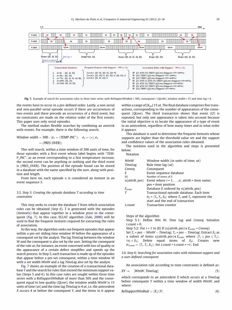
Fig. 7. Example of search for association rules in three time series with RelSupportWinRule > 50%, consequent = (QLoW), window width = 15 and time-lag = 4.
F.J. Martínez-de-Pisón et al. / Computers & Industrial Engineering 63 (2012) 22–36 29
the events have to occur in a pre-defined order. Lastly, a non-serialand non-parallel serial episode occurs if there are occurrences oftwo events and these precede an occurrence of a third event, butno constraints are made on the relative order of the first events.This paper uses only serial episodes.
The method makes flexible searches by combining an asteriskwith events. For example, there is the following search:
Window width ¼ 300 : he1 ¼ ðTEMP INC�Þ; e2 ¼ ð�Þ; e3
¼ ðPRES OVERÞi
This will search, within a time window of 300 units of time, forthose episodes with a first event whose label begins with ‘‘TEM-P_INC’’, as an event corresponding to a fast temperature increase,the second event can be anything or nothing and the third eventis (PRES_OVER). The position of the episode found can be storedin a database with the name specified by the user, along with posi-tion and length.
From here on, each episode a is considered an itemset in anevent sequence S.
3.5. Step 5: Creating the episode database T according to timeconstraints
This step seeks to create the database T from which associationrules can be obtained (Step 6). T is generated with the episodes(itemsets) that appear together in a window prior to the conse-quent (Fig. 7). In this case, ECLAT algorithm (Zaki, 2000) will beused to find the frequent itemsets required for extracting the rulesof association.
In this way, the algorithm seeks out frequent episodes that appearwithin a pre-set sliding time window W before the appearance of aconsequent set by the analyst. The lag TimeLag between the windowW and the consequent is also set by the user. Setting the consequentof the rule as, for instance, an event concerned with loss of quality orthe appearance of a certain defect simplifies and speeds up thesearch process. In Step 5, each transaction is made up of the episodesthat appear before a pre-set consequent, within a time window Wwith a set width WinW and a lag TimeLag also set by the analyst.
Fig. 7 shows an example of the creation of a transactional data-base T and the search for rules that exceed the minimum support va-lue (Steps 5 and 6). In this case rules are sought within three timeseries with a RelSupportWinRule of more than 50% and the conse-quent equal to low quality (QLow); the window width WinW is 15units of time (ut) and the time lag TimeLag is 4 ut, i.e. the antecedentX occurs 4 ut before the consequent Y, and the items in it appear
within a range of |Xtot| 15 ut. The final database comprises five trans-actions, corresponding to the number of appearances of the conse-quent (QLow). The third transaction shows that event (I2) isrepeated, but only one appearance is taken into account becausethe initial objective is to locate the appearance of a type of eventin an antecedent, regardless of how many times and in what orderit appears.
This database is used to determine the frequent itemsets whosesupports are higher than the threshold value set and the supportand confidence values of the association rules obtained.
The notation used in the algorithm and steps is presentedbelow.
Notation
WinW
Window width (in units of time, ut) TimeLag Rule time-lag (ut) Conseq Consequent E Event sequence database |E| Number of items of Eei(attrib, pos)
Event where i = 1, . . . ,n; attrib = item name;pos = item positionEorder
Database E ordered by ei(attrib, pos) T Transactional episode database. Each itemtrj = hTs, Te, Eki where Ts and Te represent thestart and the end of transaction
t.count
Transaction counterSteps of the algorithmStep 5.1: Define Win W, Time Lag and Conseq. Initialize
t.count = 0.Step 5.2: For i = 1 to |E| If (ei(attrib, pos) e Eorder = Conseq)Set Ts = pos �WinW � TimeLag; Te = pos � TimeLag; Extract Ek asa subset of items ej(attrib, pos) e Eorder where ðTs 6 pos 6 TeÞ;8ej 2 Ek; Delete equal items of Ek; Creates newtrtcount ¼ hTs; Te; Eki; Set t.count = t.count = +1; End3.6. Step 6: Searching for association rules with minimum support anda user-defined consequent
An association rule according to time constraints is defined as:
XY ) ½WinW; TimeLag� ð5Þ
which corresponds to an antecedent X which occurs at a TimeLagbefore consequent Y within a time window of width WinW, andwhere:
RelSupportWinRule ¼ jXj=jY j ð6Þ
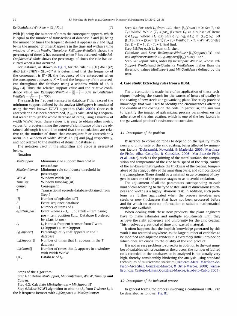
30 F.J. Martínez-de-Pisón et al. / Computers & Industrial Engineering 63 (2012) 22–36
RelConfidenceWinRule ¼ jXj=jXtot j ð7Þ
with |Y| being the number of times the consequent appears, whichis equal to the number of transactions of database T and |X| beingthe number of times the frequent itemset X appears in T and |Xtot|being the number of times X appears in the time and within a timewindow of width WinW. Therefore, RelSupportWinRule shows thepercentage of times X has occurred when Y has occurred, while Rel-ConfidenceWinRule shows the percentage of times the rule has oc-curred when X has occurred.
For instance, as shown in Fig. 7, for the rule ‘‘IF {(I1) AND (I2)AND (I3)} THEN {(QLow)}’’ it is determined that the frequency ofthe consequent is |Y = 5|, the frequency of the antecedent whenthe consequent appears is |X| = 3 and the frequency of the anteced-ent throughout the database using a window width of 15 is|Xtot = 4|. Thus, the relative support value and the relative confi-dence value are ResSupporWinRule ¼ jXjjY j ¼ 3
5 ¼ 60% RelConfidenceWinRule ¼ jXj
jXtot j ¼34 ¼ 75%.
The search for frequent itemsets in database T that exceed theminimum support defined by the analyst MinSupport is conductedusing the well-known ECLAT algorithm (Zaki, 2000). Once eachantecedent X has been determined, |Xtot| is calculated by a sequen-tial search through the whole database of items, using a window ofwidth WinW. From these values it is easy to obtain other metricvalues for predetermining the degree of significance of the rule ob-tained, although it should be noted that the calculations are rela-tive to the number of times that consequent Y or antecedent Xoccur in a window of width WinW, i.e. |Y| and |Xtot| respectively,and not relative to the number of items in database T.
The notation used in the algorithm and steps is presentedbelow.
Notation
MinSupport
Minimum rule support threshold inpercentageMinConfidence
Minimum rule confidence threshold inpercentageWinW
Window width (ut) TimeLag Window time-lag (ut) Conseq Consequent T Transactional episode database obtained fromStep 5
|T| Number of episodes of T E Event sequence database |E| Number of items of E ei(attrib, pos) Event where i = 1,. . ., n; attrib = item name;pos = item position Eorder; Database E orderedby ei(attrib, pos)
Lk
Lk is the k-frequent itemset from T withLj(Support) P MinSupportLk(Support)
Percentage of Lk that appears in the Tdatabase|Lk(Support)|
Number of times that Lk appears in the Tdatabase|Lk(Count)|
Number of times that Lk appears in a windowwith width WinW[k
Lk
Database of LkSteps of the algorithmStep 6.1: Define MinSupport, MinConfidence, WinW, TimeLag andConseq.Step 6.2: Calculate MinSupItemset = MinSupport|T|Step 6.3:Use ECLAT algorithm to obtain [kLk from T where Lk is
the k-frequent itemset with Lk(Support) P MinSupItemset
Step 6.4:For each Lk from [kLk then |Lk(Count)| = 0; Set Ts = 0;Te = WinW; While (Te 6 posen
)Extract Gk as a subset of itemsgj e Eorder where ðTs 6 gjðposÞ 6 TeÞ; 8gj 2 Ek; If ðLk # GkÞ Set|Lk(Count)| = |(Count)| + 1; Ts = Ts + WinW; Te = Te + WinW; or elseSet Ts = Ts + 1; Te = Te + 1; End End.Step 6.5:For each Lk from [kLk thenCalculate and Save RelSupportWinRule = |Lk(Support)|/|Y| andRelConfidenceWinRule = |Lk(Support)|/|Lk(Count)|; End.Step 6.6:Report rules, order by Relsupport WinRule, whose Rel-Support WinRuleand RelConfience WinRuleare higher than thethreshold values MinSupport and MinConfidence defined by theuser.
4. Case study: Extracting rules from a HDGL
The presentation is made here of an application of these tech-niques involving the search for the causes of losses of quality inthe coating of new steels at a galvanizing plant. The study providedknowledge that was used to identify the circumstances affectingthe quality of the coating on the coils. In particular, the aim wasto identify the impact of galvanizing process parameters on theadherence of the zinc coating, which is one of the key factors inthe galvanized product’s resistance to corrosion.
4.1. Description of the problem
Resistance to corrosion tends to depend on the quality, thick-ness and uniformity of the zinc coating, being affected by numer-ous factors (Dobrzanski, Kowalski, & Madejski, 2005; Martínez-de-Pisón, Alba, Castejón, & González, 2006; Martínez-de-Pisónet al., 2007), such as the priming of the metal surface, the compo-sition and temperature of the zinc bath, speed of the strip, controlof the air-knives that regulate the thickness of the coating, temper-ature of the strip, quality of the annealing cycle, and composition ofthe atmosphere. There should be a minimal or zero content of oxy-gen in each one of the process stages so as to avoid oxidation.
The adjustment of all the parameters corresponding to eachkind of coil according to the type of steel and its dimensions (thick-ness and width) is a highly laborious task. In addition, such prob-lems are further aggravated when the process involves newsteels or new thicknesses that have not been processed beforeand for which no accurate information or suitable mathematicalmodels are available.
When dealing with these new products, the plant engineershave to make estimates and multiple adjustments until theyachieve the right adherence and uniformity for the zinc coating.This involves a great deal of time and wasted material.
It often happens that the implicit knowledge generated by thiswork is not recorded anywhere, as the large number of variables tobe modified and adjusted renders it is extremely difficult to decidewhich ones are crucial to the quality of the end product.
It is not an easy problem to solve, for in addition to the vast num-ber of variables with a bearing on the process, the number of faultedcoils recorded in the databases to be analyzed is not usually veryhigh, thereby considerably hindering the analysis using standardtechniques of multivariate statistics (Ordieres-Meré, Martínez-de-Pisón-Ascacíbar, González-Marcos, & Ortiz-Marcos, 2008; Pernía-Espinoza, Castejón-Limas, González-Marcos, & Lobato-Rubio, 2005).
4.2. Description of the industrial process
In general terms, the process involving a continuous HDGL canbe described as follows (Fig. 8):
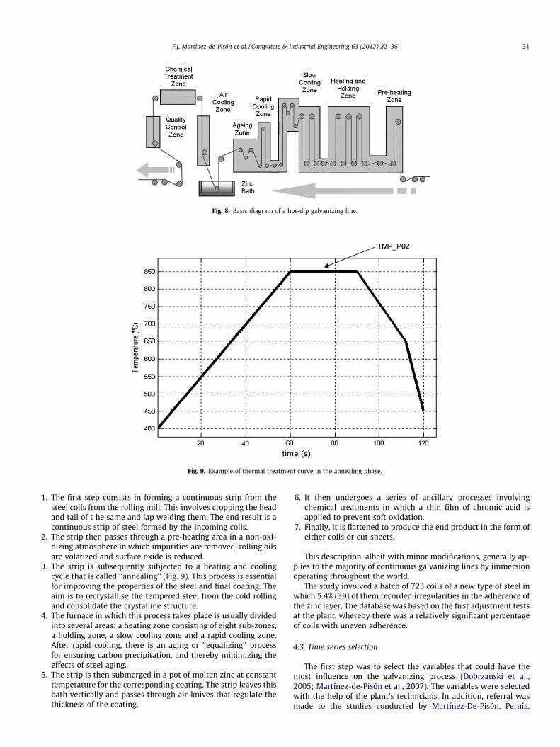
Fig. 9. Example of thermal treatment curve in the annealing phase.
Fig. 8. Basic diagram of a hot-dip galvanizing line.
F.J. Martínez-de-Pisón et al. / Computers & Industrial Engineering 63 (2012) 22–36 31
1. The first step consists in forming a continuous strip from thesteel coils from the rolling mill. This involves cropping the headand tail of t he same and lap welding them. The end result is acontinuous strip of steel formed by the incoming coils.
2. The strip then passes through a pre-heating area in a non-oxi-dizing atmosphere in which impurities are removed, rolling oilsare volatized and surface oxide is reduced.
3. The strip is subsequently subjected to a heating and coolingcycle that is called ‘‘annealing’’ (Fig. 9). This process is essentialfor improving the properties of the steel and final coating. Theaim is to recrystallise the tempered steel from the cold rollingand consolidate the crystalline structure.
4. The furnace in which this process takes place is usually dividedinto several areas: a heating zone consisting of eight sub-zones,a holding zone, a slow cooling zone and a rapid cooling zone.After rapid cooling, there is an aging or ‘‘equalizing’’ processfor ensuring carbon precipitation, and thereby minimizing theeffects of steel aging.
5. The strip is then submerged in a pot of molten zinc at constanttemperature for the corresponding coating. The strip leaves thisbath vertically and passes through air-knives that regulate thethickness of the coating.
6. It then undergoes a series of ancillary processes involvingchemical treatments in which a thin film of chromic acid isapplied to prevent soft oxidation.
7. Finally, it is flattened to produce the end product in the form ofeither coils or cut sheets.
This description, albeit with minor modifications, generally ap-plies to the majority of continuous galvanizing lines by immersionoperating throughout the world.
The study involved a batch of 723 coils of a new type of steel inwhich 5.4% (39) of them recorded irregularities in the adherence ofthe zinc layer. The database was based on the first adjustment testsat the plant, whereby there was a relatively significant percentageof coils with uneven adherence.
4.3. Time series selection
The first step was to select the variables that could have themost influence on the galvanizing process (Dobrzanski et al.,2005; Martínez-de-Pisón et al., 2007). The variables were selectedwith the help of the plant’s technicians. In addition, referral wasmade to the studies conducted by Martínez-De-Pisón, Pernía,

Table 1Sections within the HDGL.
Area Description
Pre-heating (PRE) Strip pre-heating and cleaning areaHeating: sub-areas 1–8 (01–08) Sub-areas 1–8 of the heating area of the furnace, where the strip temperature is raised to around 850 �CHolding: sub-areas 9 and 10 (09–10) Area where the strip temperature is held around 850 �C: Sub-areas 9 and 10Slow cooling (ENL) Area where the strip is cooled slowly to 600–650 �CRapid cooling (ENR) Area where the strip is cooled rapidly to 400–450 �CAging (IGU) Area where the strip temperature is equalized before being dipped into the zinc potZinc pot (BATH) Molten zinc bath dipping areaEqualizer (TRM) Equalizer areaGeneral (–) Parameters which are constant throughout the HDGL
Table 2Main groups of variables.
Name Type Description
CODE Nominal Coil codeCON_H2 Numeric H2 concentration in the air in area xxCON_O2 Numeric O2 concentration in the air in area xxTMP_PR Numeric Dew point temperature in that areaZxx_TMP Numeric Temperature of area xxTMP_Pxx Numeric Strip temperature measured with pyrometer xx in
each process areaTHICK,
WIDTHNumeric Steel strip thickness and width
SPD Numeric Strip feed rate (m/min)BATH_TMP Numeric Zinc bath temperatureCMP_BATH Numeric Chemical composition of zinc bath. Percentages of
main chemical elements in bathCMP_STEEL Numeric Chemical composition of the steel strip.
Percentages of main chemical elementsADHERENCE Binary Whether zinc coating adherence is within
tolerances (0) or not (1)
32 F.J. Martínez-de-Pisón et al. / Computers & Industrial Engineering 63 (2012) 22–36
Jiménez-Macías, and Fernández, 2010; Martínez-De-Pisón, Pernía,González, López-Ochoa, and Ordieres (2010); and Martínez-De-Pisón, Celorrio, Pérez-De-La-Parte, and Castejón (2011).
The selected variables corresponded to measurements taken ineach one of the process zones (Table 1). For each one of thesezones, the time series were recorded for the following: air compo-sition (in percentage of H2 and O2), the temperature in each zone,the temperature of the steel strip recorded at several points and ta-ken using pyrometers, strip velocity and dewpoint temperature invarious process zones, amongst others (Table 2). In addition, inclu-sion was made of the dimensions of each coil (width and thick-ness), chemical composition of the steel in each coil processed, aswell as the temperature and composition of the zinc bath. All themeasurements were taken linearly every 100 m along the steelstrip. Accordingly, each value for each time series correspondedto the mean of the readings taken for 100 m of steel strip.
The output variable was a binary value of ‘‘GOOD’’ or ‘‘BAD’’ thatindicated whether the thickness of the zinc coating was acceptable(‘‘GOOD’’) or not (‘‘BAD’’).
4.4. Pre-processing and segmentation of the time series (steps: 1, 2, 3and 4)
Following the selection of the more representative process vari-ables, a battery of filters was selected for each time series. The fil-tering of each time series was designed to extract the basic form ofthe same in order to facilitate the subsequent process of extractingepisodes.
Basically, the choice for most of the variables involved filtersthat screened below a threshold value in order to eliminate zerosor very low values due to data gathering failures or sensor deficien-cies. Filters of this kind use the last valid value recorded at instant
t � 1 to replace zero values or those below a set threshold for in-stant t. In addition, inclusion was made in most cases of sliding-window filters with Gaussian functions of widths between 5 and20 in order to smooth the final series and obtain the signal’s basicshape. Figs. 2 and 3 show two examples of filtering applied to twoprocess temperatures, respectively.
Once the basic shapes had been obtained for each one of thetime series, the next step involved obtaining the most significantmaxima and minima with a view to extracting the most significantepisodes. In most variables, the most appropriate values of Raccording to (1) and (2) ranged between 1.001 and 1.009. Theaim was to extract the truly significant maxima and minima foreach time series.
The next step was to extract the characteristic events from eachone of them. Table 3 shows the 120 types of significant eventswhich were deemed useful for seeking knowledge according toFig. 4.
For simplification purposes, each episode corresponded to a sin-gle event extracted from the 120 defined in Table 3. Therefore, Step4 in the method was not taken as there was insufficient back-ground to successfully form the complex sequences of eventscalled episodes. In spite of this, the method is fully valid for thepractical case studied.
In general, some episodes extracted correspond to momentswhen the time series were higher or lower than a specific value:for example when the concentrations of O2 and H2 were below athreshold or when the area temperature, the zinc bath tempera-ture, the strip temperature or the strip feed rate were above or be-low a certain value. Other episodes are moments when variablessuch as the area temperature, the strip temperature or the stripfeed rate fluctuated significantly (not horizontal episodes,NOT_HOR).
For the chemical compositions of the zinc bath and the type ofsteel in the coils, events were generated only in those cases whenthe mean Euclidian distance of each composition in each coil wassignificantly high, i.e. when the steel detected in the coils or thezinc bath composition was very different from usual.
The events in Table 3 and the values of the search parametersfor each one of them were defined with the help of on-site techni-cians. In compliance with the confidentiality agreement reachedwith the company, the final values of the parameters used forextracting the events cannot be disclosed.
4.5. Creating the episode database T (Step: 5)
Once all the significant episodes or itemsets had been found foreach time series analyzed, the episode database T was built, witheach transaction corresponding to the itemsets that appeared ata given moment, within a time window width of 80 ut (8000 stripmeters), with the consequent set to ‘‘ADHERENCE_BAD’’ and atime-lag of zero (Fig. 10).

Table 3Types of episode defined.
Name Number Type Description
CON_H2_Zxx_BELOW 10 BELOW H2 concentration in the air in zone x below a thresholdCON_O2_Zxx_BELOW 10 BELOW O2 concentration in the air in zone x below a thresholdZxx_TMP_OVER 10 OVER Temperature of area xx over a thresholdZxx_TMP_BELOW 10 BELOW Temperature of area xx below a thresholdZxx_TMP_NOT_HOR 10 NOT_HOR Temperature of area xx with big changes (not homogeneous)TMP_Pxx_OVER 11 OVER Strip temperature measured with pyrometer xx over a thresholdTMP_Pxx_INC 11 INC Strip temperature measured with pyrometer xx with high incrementTMP_Pxx_DEC 11 DEC Strip temperature measured with pyrometer xx with high decrementTMP_Pxx_BELOW 11 BELOW Strip temperature measured with pyrometer xx below a thresholdTMP_Pxx_NOT_HOR 11 NOT_HOR Strip temperature measured with pyrometer xx with big changes (not homogeneous)THICK_OVER 1 OVER Steel strip thickness over a thresholdTHICK_BELOW 1 BELOW Steel strip thickness below a thresholdWIDTH_OVER 1 OVER Steel strip width over percentile 95WIDTH_BELOW 1 BELOW Steel strip width below percentile 5SPD_OVER 1 OVER Strip feed rate over a thresholdSPD_BELOW 1 BELOW Strip feed rate below a thresholdSPD_INC 1 INC Strip feed rate with high incrementSPD_DEC 1 DEC Strip feed rate with high decrementSPD_NOT_HOR 1 NOT_HOR Strip feed rate with big changes (not homogeneous)BATH_TMP_OVER 1 OVER Zinc bath temperature over a thresholdBATH_TMP_BELOW 1 BELOW Zinc bath temperature below a thresholdBATH_TMP_NOT_HOR 1 NOT_HOR Zinc bath temperature big changes (not homogeneous)BATH_CMP__OVER 1 OVER Mean of Euclidean distance of chemical composition of zinc bath to other coils over a thresholdSTEEL_CMP_OVER 1 OVER Mean of Euclidean distance of the steel. Percentages of main chemical elements: Fe, Mn, Al, Ni, etc. to other coils over a
thresholdADHERENCE_BAD 1 LABEL Zinc coating adherence outside tolerances
F.J. Martínez-de-Pisón et al. / Computers & Industrial Engineering 63 (2012) 22–36 33
In other words, whenever a failure was detected due to the pooradherence of the zinc coating (ADHERENCE_BAD), a search wasmade for those episodes or items recorded over the preceding8000 m of strip. The episodes found, which had occurred just be-fore the appearance of the poor adherence, were stored in T.
As the poor adherence of the zinc coating affected 39 steel coils,by the end of the process the T database consisted of 39 rows or
Fig. 10. Example of CONOTOO
lists of major episodes occurring prior to the zinc coating’s adher-ence failure.
4.6. Searching for association rules (Step 6)
The search process for frequent itemsets or episodes for theantecedent was performed with the ECLAT algorithm and a
L rule extraction window.

34 F.J. Martínez-de-Pisón et al. / Computers & Industrial Engineering 63 (2012) 22–36
minimum RelSupportWinRule of 50%. There were 64 frequent item-sets or episodes with a RelSupportWinRule higher than 50%. Table 4shows the first 20 frequent itemsets ordered from larger to smalleraccording to the RelSupportWinRule and accompanied by the Rel-ConfidenceWinRule for each one of the rules extracted.
The frequent itemsets or episodes obtained were analyzed visu-ally in order to obtain useful hidden knowledge that would explainthe causes of the faults recorded on the steel coils. The analysis ofthe results considered the values of both RelSupportWinRule andRelConfidenceWinRule, as well as the true significance of each oneof the rules extracted.
Table 4First 20 rules extracted (arranged by support). Highlighted in bold are the twointeresting rules with the highest RelConfidenceWinRule.
Num. Items RelSupportWinRule RelConfidenceWinRule
1 {Z06_TMP_BELOW} 0.77 0.532 {TMP_P02_BELOW} 0.69 0.453 {BATH_TMP_BELOW
SPD_DECZ06_TMP_BELOW} 0.67 0.76
4 {BATH_TMP_BELOWZ06_TMP_BELOW} 0.67 0.60
5 {BATH_TMP_BELOWSPD_DEC} 0.67 0.62
6 {SPD_DECZ06_TMP_BELOW} 0.67 0.62
7 {Z06_TMP_BELOWTMP_P02_BELOW} 0.67 0.45
8 {SPD_DEC} 0.67 0.609 {BATH_TMP_BELOW} 0.67 0.72
10 {BATH_TMP_BELOWSPD_DECZ06_TMP_BELOWTMP_P02_BELOW} 0.62 0.55
11 {BATH_TMP_BELOWSPD_DECZ06_TMP_BELOWSPD_NOT_HOR} 0.62 0.55
12 {BATH_TMP_BELOWSPD_NOT_HORMP_P02_BELOWTMP_P02_BELOW} 0.62 0.55
13 {BATH_TMP_BELOWZ06_TMP_BELOWSPD_NOT_HORTMP_P02_BELOW} 0.62 0.72
14 {BATH_TMP_BELOWZ06_TMP_BELOWSPD_NOT_HOR} 0.62 0.73
15 {BATH_TMP_BELOWSPD_NOT_HORTMP_P02_BELOW} 0.62 0.80
16 {BATH_TMP_BELOWSPD_DECSPD_NOT_HOR} 0.62 0.58
17 {SPD_DECZ06_TMP_BELOWSPD_NOT_HORTMP_P02_BELOW} 0.62 0.55
18 {SPD_DECZ06_TMP_BELOWSPD_NOT_HOR} 0.62
19 {SPD_DECSPD_NOT_HORTMP_P02_BELOW} 0.62 0.65
20 {Z06_TMP_BELOWSPD_NOT_HORTMP_P02_BELOW} 0.62 0.70
Table 4 shows that the majority of the frequent episodes foundinvolve combinations of a small group of events {(Z06_TMP_BE-LOW), (TMP_P02_BELOW), (BATH_TMP_BELOW), (SPD_DEC,Z06_TMP_BELOW5) and (SPD_NOT_HOR)} which appear in almostall the rules and which form redundant rules, albeit with differentvalues of RelConfidenceWinRule. It should be remembered that Rel-ConfidenceWinRule explains the number of times the antecedentappears when the consequent occurs, in this case faulty zinc coat-ing (ADHERENCE_BAD), divided by the number of times the ante-cedent appears in the entire database, although always within awindow with a previously defined width, which in this case is 80ut (equivalent to 8000 strip meters). Accordingly, a low value indi-cates a weak relationship between the antecedent and the conse-quent as the antecedent appears regardless of whether or not theconsequent occurs; by contrast, a high value of RelConfidenceWin-Rule indicates a cause cause–effect relationship between the ante-cedent and the consequent. Highlighted in bold are the two rules (3and 15) with the highest RelConfidenceWinRule and, therefore, themost interesting ones to analyze:
[3]
IF {(BATH_TMP_BELOW) & (SPD_DEC) &(Z06_TMP_BELOW)} THEN ADHERENCE_BAD WinW = 80, TimeLag = 0 (RelSupportWinRule = 67%,RelConfidenceWinRule = 76%)[15]
IF {(BATH_TMP_BELOW) & (SPD_NOT_HOR) &(TMP_P02_BELOW)} THEN ADHERENCE_BAD WinW = 80, TimeLag = 0 (RelSupportWinRule = 62%,RelConfidenceWinRule = 80%)The first knowledge rule reveals that when the temperature in
the zinc bath is low (BATH_TMP_BELOW), the temperature in zone6 of the furnace is also low (Z06_TMP_BELOW) and the strip feedrate falls sharply (SPD_DEC), coinciding with faulty zinc coating(ADHERENCE_BAD). This occurred with 67% of database T and theconsequent was fulfilled 76% of the times when the antecedent ap-peared. In other words, this rule is fulfilled 67% of the times therehas been an adherence fault. Furthermore, it is a rule with a highconfidence level, as 76% of the times the antecedent has occurredthere has also been an adherence fault.The second knowledge rule indicates that sudden changes invelocity (SPD_NOT_HOR) together with low zinc bath temperatures(BATH_TMP_BELOW) and low strip temperatures at the furnaceoutlet (TMP_P02_BELOW) lead to errors in the zinc coating in 62%of database T. This was fulfilled 80% of the time. In other words,62% of the faulted coils have been preceded by the episodes de-scribed in this rule’s antecedent. In addition, 80% of the times theantecedent has occurred there have also been coating faults onthe coils.
As with most instances of research into association rules, mostof the other rules involved episodes similar to rules 3 and 15 butwith a lower RelConfidenceWinRule, so they were deemed to beweaker than the former two.
Finally, other rules such as the first and second ones were notconsidered important as their RelConfidenceWinRule values weretoo low.
In short, the two rules extracted, with high values for RelSuppor-tWinRule and RelConfidenceWinRule, had useful hidden knowledgefor identifying the causes of adherence failure in a high percentageof defective coils. Accordingly, the identification of the rules’ mostcharacteristic episodes enabled on-site technicians to know whichparts of the process should be the focus of corrective and surveil-lance actions in order to reduce the adherence defects affectingthe zinc coating.

F.J. Martínez-de-Pisón et al. / Computers & Industrial Engineering 63 (2012) 22–36 35
5. Conclusions
This paper presents an experiment based on simple pre-pro-cessing, segmentation and a search for hidden knowledge on. thebasis of time series that can be easily applied to the enhancementof production processes. The pre-processing and segmentation oftime series linked to the use of association rule algorithms maybe extremely useful when searching for hidden knowledge in thedata logs of industrial processes, which may help to improve pro-duction processes.
The experiment has shown that techniques of this nature de-pend heavily on the expertise of the analyst and that the ‘‘humanfactor’’ is vital at all the stages proposed in this methodology. Aninteresting improvement may involve using the logic of fuzzy asso-ciations in order to seek more flexible sequences akin to humanthought processes. The technique has been proposed for frequentepisode mining to detect the performance of network intrusiondetection systems (Luo & Bridges, 2000).
On a practical level, the conclusion drawn is that by means ofiterative and interactive adjustments of the pre-processing andsegmentation functions (filters, detection of significant maximaand minima, definition and extraction of episodes) experts can ob-tain significant rules more reliably than in fully automatic ruleextraction systems. We therefore consider it worthwhile to makethe effort required to develop tools to facilitate iteration for expertsand analysis software in all pre-processing and time series seg-mentation tasks.
All the pre-processing and segmentation algorithms for timeseries were implemented via the free statistical analysis programR (R Development Core Team, 2008) within a library called KDSer-ies. Furthermore, given the enormous effort in trial and error that isrequired at these stages, it was decided to develop a new visualtool called CONOTOOL to make these tasks easier. This tool allowsa more intuitive, speedier use of all the functions in the KDSeries li-brary. The latest available versions of both the KDSeries library andCONOTOOL can be downloaded from the CONOSER Project website:http://api.unirioja.es/conoser.
It is worth noting that tools of this kind can be used not only forextracting knowledge from industrial processes but also extrapo-lated, with the same degree of success, to other fields such as theenvironment, network systems, business, and marketing.
Acknowledgements
The authors thank the ‘‘Dirección General de Investigación’’ ofthe Spanish Ministry of Education and Science for the financialsupport of Project DPI2006-03060, Universidad de La Rioja andBanco Santander for the support of Project API11/13 and the Euro-pean Union for Project RFS-PR-06035.
Finally, the authors also thank the Autonomous Government ofLa Rioja for support through its 3rd R&D&i Plan within Project FO-MENTA 2010/13.
References
Abdel-Aal, R. E. (2008). Univariate modeling and forecasting of monthly energydemand time series using abductive and neural networks. Computers &Industrial Engineering, 54(4), 903–917.
Agrawal, R., & Srikant, R. (1994). Fast algorithms for mining association rules. In:Proceedings of the 20th international conference on very large databases (pp. 487–499). Santiago, Chile.
Alfonso-Cendón, J., González-Marcos, A., Castejón-Limas, M., & Ordieres-Meré, J. B.(2010). A multi-agent data mining system for defect forecasting in adecentralized manufacturing environment. Computational Intelligence inSecurity for Information Systems, 85(2010), 43–50. doi:10.1007/978-3-642-16626-6_5.
Bellazi, R., Larizza, C., Magni, P., & Bellazi, R. (2005). Temporal data mining for thequality assessment of hemodialysis services. Artificial Intelligence in Medicine,34, 25–39.
Bettini C., Wang, X. S., & Jajodia, S. (1996). Testing complex temporal relationshipsinvolving multiple granularities and its applications to Data Mining. InProceedings of the 15th ACM symposium principles of database systems (pp. 68–78). Montreal, Quebec, Canada.
Bettini, C., Wang, X. S., & Jajodia, S. (1998). Mining temporal relationships withmultiple granularities in time sequences. Data Engineering Bulletin, 21(1),32–38.
Bishop, C. M. (2006). Pattern recognition and machine learning. London: Springer.Buddhakulsomsiri, J., & Zakarian, A. (2009). Sequential pattern mining algorithm for
automotive warranty data. Computers & Industrial Engineering, 57, 137–147.Chen, G., Wei, Q., Liu, D., & Wets, G. (2002). Simple association rules (SAR) and the
SAR-based rule discovery. Computers & Industrial Engineering, 43(4), 721–733.Chen, Y.-C., Jiang, J.-C., Peng, W.-C., & Lee, S.-Y. (2010). An efficient algorithm for
mining time interval-based patterns in large databases. In Proceedings of the19th ACM international conference on information and knowledge management,Proceedings (pp. 49–58), Toronto, ON, Canada.
Chen, Y.-W., & Chai, T.-Y. (2010). Research and application on temperature controlof industry heating furnace. Journal of Iron and Steel Research, 22(9), 53–57.
Core, B., & Goethals, B. (2010). Mining association rules in long sequences. LectureNotes in Computer Science, 6118 LNAI (PART1), pp. 300–309.
Das, G., Gunopulos, D., & Mannila, H. (1997). Finding similar time series. In:Proceedings of the first European symposium on principles and practice ofknowledge discovery in databases (pp. 88–100).
Das, G., Lin, K.I., Mannila, H., Renganathan, G., & Smyth, P. (1998). Rule discoveryfrom time series. In Proceedings of the fourth ACM SIGKDD internationalconference on knowledge discovery and data mining (pp. 16–22). AAAI Press.
Dasha, P. K., Nayaka, M., Senapatia, M. R., & Lee, I. W. C. (2007). Mining forsimilarities in time series data using wavelet-based feature vectors and neuralnetworks. Engineering Applications of Artificial Intelligence, 20(2), 185–201.
Gauri, S. K., & Chakraborty, S. (2006). Feature-based recognition of control chartpatterns. Computers & Industrial Engineering, 51(4), 726–742.
Dobrzanski, L. A., Kowalski, M., & Madejski, J. (2005). Methodology of themechanical properties prediction for the metallurgical products from theengineering steels using the artificial intelligence methods. Journal of MaterialsProcessing Technology, 164–165, 1500–1509.
Dong, Z., Li, H., & Shi, Z. (2004). An efficient algorithm for mining inter-transactionassociation rules in multiple time series. Journal of Computer Science, 31(3),108–111.
Dorr, D. H., & Denton, A. M. (2009). Establishing relationships among patterns instock market data. Data and Knowledge Engineering, 68(3), 318–337.
Essafi, M., Delorme, X., Dolgui, A., & Guschinskaya, O. (2010). A MIP approach forbalancing transfer line with complex industrial constraints. Computers &Industrial Engineering, 58(3), 393–400.
Feng, L., Dillon, T., & Liu, J. (2001). Inter-transactional association rules for multi-dimensional contexts for prediction and their applications to studyingmeteorological data. Data & Knowledge Engineering, 37(1), 85–115.
Ferreiro, S., Sierra, B., Irigoien, I., & Gorritxategi, E. (2011). Data Mining for qualitycontrol: Burr detection in the drilling process. Computer & Industrial Engineering,60(4), 801–810.
Fink, E., & Pratt, K. B. (2004). Indexing of compressed time series. In M. Last, A.Kandel, & H. Bunke (Eds.), Data mining in time series databases (pp. 51–78). NewYork: World Scientific.
Fu, T.-C. (2011). A review on time series data mining. Engineering Applications ofArtificial Intelligence, 24(1), 164–181.
Gauri, S. K., & Chakraborty, S. (2009). Recognition of control chart patterns usingimproved selection of features. Computers & Industrial Engineering, 56(4),1577–1588.
Haji, A., & Assadi, M. (2009). Fuzzy expert systems and challenge of new productpricing. Computers & Industrial Engineering, 56(2), 616–630.
Han, J., & Kamber, M. (2006). Data mining: Concepts and techniques. San Francisco,CA: Morgan Kaufmann.
Hand, D., Mannila, H., & Smyth, P. (2001). Principles of data mining. Cambridge, MA:MIT Press [London, England].
Harms, S., Deogun, K., Saquer, J., & Tadesse, T. (2001). Discovering representativeepisodal association rules from event sequences using frequent closed episodesets and event constraints. In Proceedings of the 2001 IEEE internationalconference on data mining (pp. 603–606).
Harms, S. K, Deogun, J., & Tadesse, T. (2002). Discovering sequential associationrules with constraints and time lags in multiple sequences. In Proceedings of the2002 international symposium on methodologies for intelligent systems (Vol. 2366,pp. 432–441). Berlin, Heidelberg.
Harms, S., Li, D., Goddard, S., & Waltman, W. (2003). Time series data mining in ageospatial decision support system. In ACM international conference proceedingsseries (Vol. 130, pp. 1–4). Boston, MA.
Harms, S., Tadesse, T., Wilhite, D., Hayes, M., & Goddard, S. (2004). Droughtmonitoring using data mining techniques: A case study for Nebraska, USA.Natural Hazards, 33, 137–159.
Hong, K., Hong, S., & So, Y. (2009). Sequential association rules for forecasting failurepatterns of aircrafts in Korean air force. Expert Systems with Applications, 36,1129–1133.
Huang, K.-Y., & Chang, C.-H. (2007). Efficient mining of frequent episodes fromcomplex sequences. Information Systems, 33(1), 96–114.

36 F.J. Martínez-de-Pisón et al. / Computers & Industrial Engineering 63 (2012) 22–36
Huang, Y., Hsu, C., & Wanga, S. (2007). Pattern recognition in time series database: Acase study on financial database. Expert Systems with Applications, 33, 199–205.
Huang, Y., Kao, L., & Sandnes, F. (2008). Efficient mining of salinity and temperatureassociation rules from ARGO data. Expert Systems with Applications, 35, 59–68.
Keogh, E., Chu, S., Hart, D., & Pazzani, M. (2004). Segmenting time series: A surveyand novel approach. In Data Mining In Time Series Databases, 1, 1–22.
Koskal, G., Batmaz, I., & Testik, M. C. (2011). A review of data mining applications forquality improvement in manufacturing industry. Expert Systems withApplications, 38(10), 13448–13467.
Kam, P.-S., & Fu, A. W.-C., 2000. Discovering temporal patterns for interval-basedevents. In Proceedings of the 2nd international conference on data warehousingand knowledge, discovery (DaWaK’00) (pp. 317–326).
Last, M., Klein, Y., & Kandel, A. (2001). Knowledge discovery in time seriesdatabases. IEEE Transactions on Systems, Man and Cybernetics, 31(1), 160–169.
Last, M. (2004). Data mining in time series databases. Series in machine perception andartificial intelligence (Vol. 57). London: World Scientific Publishing Co. Pte. Ltd.
Lau, H. C. W., Ho, G. T. S., Chu, K. F., Ho, W., & Lee, C. K. M. (2009). Development of anintelligent quality management system using fuzzy association rules. ExpertSystems with Applications, 36(2–1), 1801–1815.
Laxman, S., & Sastry, P. S. (2006). A survey of temporal data mining. In Sadhana (Vol.31, pp. 173–198). Bangalore: Springer Indian.
Liu, C., & Teng, H. (2008). Human–computer cooperative layout design method andits application. Computers & Industrial Engineering, 55(4), 735–757.
Luo, J., & Bridges, S. M. (2000). Mining fuzzy association rules and fuzzy frequentepisodes for intrusion detection. International Journal of Intelligent Systems,15(8), 687–703.
Mannila, H., Toivonen, H., & Verkamo, A. (1997). Discovery of frequent episodes inevent sequences. Data Mining Knowledge Discovery, 1(3), 259–289.
Martínez-de-Pisón, F. J., Alba, F., Castejón, M., & González, J. A. (2006). Improvementand optimisation of hot dip galvanising line using neural networks and geneticalgorithms. Ironmaking and Steelmaking, 33, 344–352.
Martínez-de-Pisón, F. J., Ordieres, J., Pernía, A. V., & Alba, F. (2007). Reduce ofadherence problems in galvanised processes through data mining techniques.Revista de Metalurgia, 43, 325–336.
Martínez-De-Pisón, F. J., Pernía, A. V., González, A., López-Ochoa, L. M., & Ordieres, J.B. (2010a). Optimum model for predicting temperature settings on hot dipgalvanising line. Ironmaking and Steelmaking, 37, 187–194.
Martínez-De-Pisón, F. J., Pernía, A. V., Jiménez-Macías, E., & Fernández, R. (2010b).Overall model of the dynamic behaviour of the steel strip in an annealingheating furnace on a hot-dip galvanizing line. Revista de Metalurgia, 46,405–420.
Martínez-De-Pisón, F. J., Celorrio, L., Pérez-De-La-Parte, M., & Castejón, M. (2011).Optimising annealing process on hot dip galvanising line based on robustpredictive models adjusted with genetic algorithms. Ironmaking andSteelmaking, 38(3), 218–228.
Mongkolnavin, J., & Tirapat, S. (2009). Marking the close analysis in Thai BondMarket surveillance using association rules. Expert Systems with Applications, 36,8523–8527.
Moreno, M., Ramos, I., García, F. J., & Toro, M. (2008). An association rule miningmethod for estimating the impact of project management policies on softwarequality, development time and efforts. Expert Systems with Applications, 34,522–529.
Mörchen, F., Ultsch, A., & Hoos, O. (2004). Discovering interpretable muscleactivation patterns with the Temporal Data Mining Method. In J.-F. Boulicaut,F. Esposito, F. Giannotti, & D. Pedreschi (Eds.), Proceedings of the 8th European
Conference on Principles and Practice of Knowledge Discovery in Databases(PKDD’04), Lecture Notes in Computer Science (pp. 512–514).
Mörchen, F., & Ultsch, A. (2007). Efficient mining of understandable patterns frommultivariate interval time series. Data Mining and Knowledge Discovery, 15(2),181–215.
Oliver, J. J., Bexter, R. A., & Wallace, C. S. (1998). Minimum message lengthsegmentation. In: Proceedings of the Second Pacific–Asia Conference on KnowledgeDiscovery and Data Mining (pp. 222–233).
Ordieres, J. B., Martínez-de-Pisón, F. J., Castejón, M., & González, A. (2005). Datamining in industrial process. III Taller de Minería de Datos y Aprendizaje(TAMIDA 2005). Granada, Spain. ISBN 84-9732-449-8.
Ordieres-Meré, J. B., Martínez-de-Pisón-Ascacíbar, F. J., González-Marcos, A., &Ortiz-Marcos, I. (2008). Comparison of models created for the prediction of themechanical properties of galvanized steel coils. Journal of IntelligentManufacturing. doi:10.1007/s10845-008-0189-y.
Pernía-Espinoza, A. V., Castejón-Limas, M., González-Marcos, A., & Lobato-Rubio, V.(2005). Steel annealing furnace robust neural network model. Ironmaking andSteelmaking, 32, 418–426.
R Development Core Team, 2008. R: A language and environment for statisticalcomputing. R Foundation for Statistical Computing, Vienna, Austria. ISBN 3-900051-07-0.
Schmidt-Thieme, L. (2004). Algorithmic Features of ECLAT, In: Proceedings of theIEEE ICDM workshop on frequent itemset mining implementations (Vol. 126).Brighton: UK.
Su, M.-Y. (2010). Discovery and prevention of attack episodes by frequent episodesmining and finite state machines. Journal of Network and Computer Applications,33, 156–167.
Tak-chung, F. (2011). A review on time series data mining. Engineering Applicationsof Artificial Intelligence, 24(1), 164–181.
Terzi, E., & Tsaparas, P. (2006). Efficient algorithms for sequence segmentation. In2006 SIAM conference on data mining (pp. 314–325).
Triantaphyllou, E., Liao, T. W., & Iyengar, S. S. (2002). A focused issue on data miningand knowledge discovery in industrial engineering. Computers & IndustrialEngineering, 43(4), 657–659.
Tung, A., Lu, H., Han, J., & Feng, L. (1999). Breaking the barrier of transactions:Mining inter-transaction association rules. In Proceedings of the fifth ACMSIGKDD international conference on knowledge discovery and data mining (pp.297–301).
Tung, A., Lu, H., Han, J., & Feng, L. (2003). Efficient mining of inter-transactionassociation rules. IEEE Transactions on Knowledge and Data Engineering, 15(1),43–56.
Ultsch, A. (2004). Unification-based temporal grammar. Technical Report 37,Department of Mathematics and Computer Science, Philipps-University, Marburg.
Villafane, R., Hua, K. A., Tran, D., & Maulik, B. (2000). Knowledge discovery fromseries of interval events. Journal of Intelligent Information Systems, 15(1), 71–89.
Wang, B., Wang, S.-A., Du, H.-F., & Qu, P.-G. (2003). Parameter optimization incomplex industrial process control based on improved fuzzy-GA. InternationalConference on Machine Learning and Cybernetics, 4, 2512–2515.
Winarko, E., & Roddick, J. (2007). ARMADA – An algorithm for discovering richerrelative temporal association rules from interval-based data. Data & KnowledgeEngineering, 63, 76–90.
Zaki, M. J. (2000). Scalable algorithms for association mining. IEEE Transactions onKnowledge and Data Engineering, 12(3), 372–390.
Zhao, Q., & Bhowmick, S. (2003). Sequential pattern mining, technical report.Singapore: Nanyang Technological University.

42 Chapter 3. PUBLICATION I
16
42

Chapter 4
PUBLICATION II
Sanz-García, A., Fernández-Ceniceros, J., Fernández-Martínez, R. &
Martínez-de-Pisón, F. J. (2012). Methodology based on genetic optim-
isation to develop overall parsimony models for predicting temperature
settings on an annealing furnace, Ironmaking & Steelmaking, available
on line. DOI 10.1179/1743281212Y.0000000094.
The publisher and copyright holder corresponds to Maney Publishing, which is
the trading name of W.S.Maney & Son Ltd. The online version of this journal
are the URLs:
• http://maneypublishing.com/index.php/journals/irs/
• http://www.ingentaconnect.com/content/maney/ias
43

44 Chapter 4. PUBLICATION II
.......
44

Methodology based on genetic optimisationto develop overall parsimony models forpredicting temperature settings on annealingfurnace
A. Sanz-Garcıa, J. Fernandez-Ceniceros, R. Fernandez-Martınez andF. J. Martınez-de-Pison*
Developing better prediction models is crucial for the steelmaking industry to improve the
continuous hot dip galvanising line (HDGL). This paper presents a genetic based methodology
whereby a wrapper based scheme is optimised to generate overall parsimony models for
predicting temperature set points in a continuous annealing furnace on an HDGL. This
optimisation includes a dynamic penalty function to control model complexity and an early
stopping criterion during the optimisation phase. The resulting models (multilayer perceptron
neural networks) were trained using a database obtained from an HDGL operating in the north of
Spain. The number of neurons in the unique hidden layer, the inputs selected and the training
parameters were adjusted to achieve the lowest validation and mean testing errors. Finally, a
comparative evaluation is reported to highlight our proposal’s range of applicability, developing
models with lower prediction errors, higher generalisation capacity and less complexity than a
standard method.
Keywords: Hot dip galvanising line, Annealing furnace, Genetic algorithms, Artificial intelligence, Overall models, Parsimony criterion
List of symbolsAl, Cu, Ni, Cr, Nb chemical composition of steel,
wt-%
C, Mn, Si, S, P chemical composition of steel,wt-%
G total number of generations
I number of best individuals forearly stopping
J fitness function
P population size
q binary array for feature selectionarray
RMSE root mean squared error
T period of stability
THC1 zone 1 set point temperature(initial heating zone), uC
THC3 zone 3 set point temperature(intermediate heating zone), uC
THC5 zone 5 set point temperature (finalheating zone), uC
ThickCoil strip thickness at the annealingfurnace inlet, mm
TMPP1 strip temperature at the heatingzone inlet, uC
TMPP2 strip temperature at the heatingzone outlet, uC
TMPP2CNG strip set point temperature at theheating zone outlet, uC
V, Ti, B, N chemical composition of steel,wt-%
VelMed strip velocity inside the annealingfurnace, m min21
W complexity termWidthCoil strip width at the annealing fur-
nace inlet, mmx user-defined fraction or propor-
tiond generation defined penalty coeffi-
cientl chromosomeL population arraym weighting coefficient of complexity
terms normalisation coefficientx mutation factor
SubscriptsCI confidence interval
e elitismg current generation {1,…G}
EDMANS Group, Department of Mechanical Engineering, University of LaRioja, Logrono 26004, Spain
*Corresponding author, email [email protected]
� 2012 Institute of Materials, Minerals and MiningPublished by Maney on behalf of the InstituteReceived 31 August 2012; accepted 26 November 2012DOI 10.1179/1743281212Y.0000000094 Ironmaking and Steelmaking 2012 VOL 0 NO 0 1

tst testing dataval validation data
Superscriptsi index of each individual {1,…,P}s sorted array
IntroductionIn recent times, many authors have reported that theannealing phase has a significant influence on coatingsteel adherence in the continuous galvanising process(Fig. 1).1–3 When the steel strip receives a non-uniformheat treatment, it may lead to inadequate steel proper-ties, inconsistency in the quality of the coating layer andadditional coating problems, including surface oxidationand carbon contamination.4 The standard operatingmode on a continuous hot dip galvanising line (HDGL)usually involves determining the optimal settings toensure a suitable thermal annealing treatment for eachtype of steel coil (Fig. 2) and a correct temperaturedistribution before the zinc bath. Accordingly, propertemperature adjustment inside the continuous annealingfurnace (CAF) is the main task because the finaltemperature has to be uniform over the whole lengthof the strip and very close to a pre-established optimalvalue for the proper application of the zinc coating.However, current control systems face numerous pro-blems when dealing with new steel coils that have notbeen previously mapped. The following disadvantagesare generally found for most of these models.
First, their implementation in a galvanising linerequires the generation of one non-linear model foralmost every one of the products manufactured.
Second, model coefficients require several adjustmentsover time to adapt to new processing conditions. In thecase of data driven models, the development isconducted offline through an iterative training processusing available historical data and requiring longperiods of time.
Third, models are unable to maintain the accuracy ofoutputs for the products that have not been previouslyprocessed. Continuous variations in coil dimensions andthe chemical compositions of the steel hinder their directimplementation in a real time control system.
More research in modelling, system identification andcontrol system design is still needed to address theproblem of dealing with new steel coils that have notbeen previously mapped. In particular, enhancing thenon-linear modelling of the CAF for predicting tem-perature settings is crucial on an HDGL to improvefurnace temperature regulation and homogenise striptemperature. The main requirement is that the modelsshould efficiently learn from historical data and thenuphold accuracy in response to new operating condi-tions. To this end, resulting models need to be moreparsimonious for maximising their generalisation cap-ability. In short, even though previous research hasalready shown significant improvements,5,6 developingnew overall and parsimony prediction models is still anunresolved challenge for control systems in HDGL.
Related researchAn alternative to the model based approach is theimplementation of data driven models that take intoaccount not only the inherent non-linearities of heattreatments but also the plant operators’ know how andhistorical data.7,8 Research has revealed a growinginterest in artificial intelligence models in recent years.9
For instance, neural based models have also been widelyused for modelling steelmaking processes: forecastingbreakouts in the continuous casting of slab,10 super-vising the control of a reheating furnace,11 calculatingthe rolling force for a rolling mill process controlsystem,12 productivity, CO2 content of the top gas andSi content in a blast furnace,13 estimating sinter qualityand sinter plant performance indices in a steel plant,14
predicting mechanical properties and microstructuralevolution in hot rolled steel strip,15 etc. More particu-larly, in HDGL, Lu and Markward16 reported signifi-cant improvements using artificial neural networks forcoating control, Schiefer et al.17 presented a combina-tion of clustering and a radial basis function network to
1 Basic scheme of main process in continuous HDGL
2 Three profiles of annealing treatment with two phases
in cooling section
Sanz-Garcıa et al. Overall parsimony models for predicting temperature settings
2 Ironmaking and Steelmaking 2012 VOL 0 NO 0
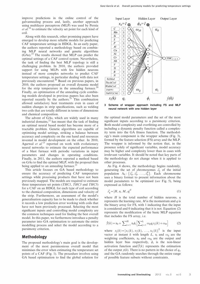
improve predictions in the online control of thegalvannealing process and, lastly, another approachusing multilayer perceptron (MLP) was used by Pernıaet al.18 to estimate the velocity set point for each kind ofcoil.
Along with this research, other promising papers haveemerged to develop more reliable models for predictingCAF temperature settings in HDGL. In an early paper,the authors reported a methodology based on combin-ing MLP neural networks and genetic algorithms(GAs).19 The results showed that MLP can predict theoptimal settings of a CAF control system. Nevertheless,the task of finding the best MLP topology is still achallenging problem. In 2010, the authors providedsupport for using MLPs with few hidden neuronsinstead of more complex networks to predict CAFtemperature settings, in particular dealing with data notpreviously encountered.20 Based on previous papers, in2010, the authors proposed an overall dynamic modelfor the strip temperature in the annealing furnace.20
Finally, an optimisation of the annealing cycle combin-ing models developed in previous papers has also beenreported recently by the authors.21 This combinationallowed satisfactory heat treatments even in cases ofsudden changes in strip specifications, such as weldingtwo coils that are totally different in terms of dimensionsand chemical composition.
The advent of GAs, which are widely used in manyindustrial domains,22 has meant that the task of findingan optimal neural based model has become more of atractable problem. Genetic algorithms are capable ofoptimising model settings, striking a balance betweenaccuracy and complexity on the one hand and resourcesinvested in model development on the other. In 2010,Agarwal et al.13 reported on work with evolutionaryneural networks to estimate the expected performanceof a blast furnace with periodic variations in inputparameters and changes in operating conditions.Finally, in 2011, the authors reported a method basedon GAs to find the optimal MLP, with the proposal thenbeing applied to an annealing furnace.21
This article focuses on GA based methodology toensure the accuracy of predicting CAF temperaturesettings while processing products that have not beenpreviously mapped. The models are required to estimatethree temperature set points (THC1, THC3 and THC5)for a CAF on an HDGL for each type of coil accordingto the chemical composition, dimensions and velocity ofthe strip. Furthermore, an assessment of the model’sgeneralisation capacity has to be made to check whetherit records a low prediction error working with coils thathave not been previously processed. Selecting the mostsignificant inputs and controlling model complexity arethe common techniques used for finding the best overallmodel. In this paper, we furthermore introduce a penaltyparameter into GA optimisation to automate the entiremodelling process and select the model according to aparsimony criterion.
MethodologyThe proposed methodology’s main goal is the develop-ment of the most parsimonious overall model thatminimises the error when estimating the temperature setpoints of a CAF (Fig. 1). The procedure involves usingGA based optimisation to find the global solution for
the optimal model parameters and the set of the mostsignificant inputs according to a parsimony criterion.Both model complexity and overfitting are controlled byincluding a dynamic penalty function called a complex-ity term into the GA fitness function. The methodol-ogy’s main component is the wrapper scheme (Fig. 3),formed by the feature selection (FS) array and the MLP.The wrapper is informed by the notion that, in thepresence solely of significant variables, model accuracymay be higher and complexity lower than in cases withirrelevant variables. It should be noted that key parts ofthe methodology do not change when it is applied toother processes.
As Fig. 4 shows, the methodology begins randomly,generating the set of chromosomes li
0 of the initialpopulation L0 : l1
0, l20, . . . , lP
0
� �. Each chromosome
uses a binary format to present information about themodel parameters to be optimised (see Fig. 5), beingexpressed as follows:
lig~ H, g, M, q½ �T (1)
where H is the total number of hidden neurons, grepresents the learning rate, M is the momentum and q isthe binary array for FS, with 1 indicating that the inputis considered and 0 indicating that it is not. Equation (2)represents the modification of the basic MLP equationthat includes the FS array, i.e.
y kð Þ~a0zXH
i~1aiwi
XL
j~1vijqjxj kð Þzvi0
h i(2)
where xj kð Þ~ x1 kð Þ, x2 kð Þ, . . . , xL kð Þ½ �T is the input
vector at instant k with length L, ai and vij are theweighting coefficients, a0 and v0j are the output andhidden layer bias respectively, wi is the non-linear
activation function and y kð Þ represents the estimationof the output y(k). There is no pattern in the choice of qi,and the GA randomly searches through the entire rangeof possible feature subsets without constraints.
3 Scheme of wrapper approach including FS and MLP
neural network with one hidden layer
Sanz-Garcıa et al. Overall parsimony models for predicting temperature settings
Ironmaking and Steelmaking 2012 VOL 0 NO 0 3

The method continues by executing the backpropaga-tion (BP) learning algorithm for each individual ofpopulation L0 to adjust MLP weights. The parametersassociated to the BP learning algorithm (g and M) arealso extracted from li
0.
Genetic algorithm optimisation and fitnessfunctionAdjusted models, which are parameterised by the list ofai and vij, are subsequently used to calculate the fitnessfunction J. In this paper, J takes into consideration notonly the criterion used for evaluating prediction errorsbut also a penalty function to discourage the complexmodels, being expressed as
J Lg
� �~RMSEval Lg
� �zd gð ÞsW Lg
� �(3)
where W is the complexity term calculated as the sum ofsquares of the weighting coefficients {ai, vij}, s is acombined reduction/normalisation coefficient to makeproportional W to RMSE and is given by
s~m ming RMSEval Lg
� �� �=ming W Lg
� �� �� �(4)
where W and RMSEval are both the minima fromcurrent generation g, and m is a reduction term used toweigh the relevance of the complexity term against theerrors. The generation defined penalty coefficient d(g) isincluded in equation (3) to represent the differentimpacts the weighting coefficients ai and vij have onthe fitness function, being given as follows
d gð Þ~ 1
1ze{ g{Gxgð Þh i (5)
where xg is a user defined fraction of G ranging from 0?1to 0?9 that represents the generation where d(g) is 50% ofits final value. As Fig. 6 shows, the values of xg affect thenumber of generations in which the complexity term isstarting to modify the fitness function J. This timeinstant is crucial because the evolution of RMSEval
makes their values lower at the beginning of theoptimisation search. In sum, the less complex a modelis and the more significant the selected inputs are, thelower J(Lg) will be. After all the models in generation gare assigned to their associated J, the population Lg issorted by increasing J values into Le
g.
The evolutionary process under the principles ofselection, crossover and mutation is then carried out to
4 Flowchart for GA based optimisation procedure
5 Binary chromosome lig: H is integer valued, g and M
are real valued, and qi is binary coded
6 Comparison of generation defined penalty functions
d(g) for different values of xg
Sanz-Garcıa et al. Overall parsimony models for predicting temperature settings
4 Ironmaking and Steelmaking 2012 VOL 0 NO 0

allow chromosomes and associated models to evolvetowards better solutions.
First, the best individuals Lg[1:Pe] are selected asparents for creating the next generation Lgz1 accordingto J(Lg) and elitism percentage xe. The rest Lg[Pe:P] ofthe population g is discarded.
A crossover operator is then applied between thepreviously selected individuals Lgz1[1:Pe] to completethe new population Lgz1[Pez1:P] with (P2Pe) newindividuals.
Finally, any new chromosomes in Lgz1[1:P] may bechanged through a bitwise mutation process. Thisgenetic operator considers each gene separately andallows each bit to flip with a very low rate probabilitygiven by x.
This is an iterative process that ends when themaximum number of generations has been reached, Jis lower than a pre-established threshold or before anearly stopping criterion (ESC) is satisfied. Finally, thegeneralisation ability of the final model is evaluatedusing a testing dataset consisting of new types of steelcoils with a different chemical composition, width,thickness, etc. It is important to note that the optimisa-tion process might be repeated over time to add newcollected data to the initial database, with plantengineers controlling the process either automaticallyor manually.
Early stopping criterion for GAThe confidence interval (CI) at a certain percentage xCI
represents the range of values of a variable for which thedifference between the variable and its estimation is notstatistically significant at a (12xCI) confidence level(CL). As the standard deviation Sn of a variable is ameasure of its spread that is normally reported by amean, those cases that meet the CL interval may beconsidered ‘steady cases’ in terms of the low variation inthe values of the variable. Based on this approach, anESC is proposed using (12xCI) values to define aninterval in which the Sn of the validation model errorRMSEval should be included to be considered a ‘steadygeneration’ for I best individuals of a generation. Thenumber of generations forming the period of stability Tis stated as the xT percentage of the total number ofgenerations. The criterion is based mainly on a practicalprocedure that searches the first subset of T generationsin which I best individuals go through with having theirCL lower than a low percentage xVAL of the value of
max RMSEvalð Þ{min RMSEvalð Þ½ �. All threshold valuesshould be adjusted after an initial experimental analysisof the evolution of the error RMSEval over severalgenerations.
Data processing and datasetsTemperature set points and all the other variables weremeasured on an HDGL operating in the north of Spain.The raw database was initially formed by 56 284observations sampled every 100 m along the strip for atotal number of 2436 steel coils of different chemicalcompositions and under different operating conditions.In 2003, Martınez-de-Pison preprocessed the data toimprove the subsequent modelling process, and severalattributes were removed after recording a high correla-tion with others or for not having enough metallurgicalrelevance in the opinion of the plant experts.23 Thepreprocessed database was formed by a total number of48 017 instances with 19 inputs and three outputs. Theoutputs are the furnace’s three main temperature setpoints THC1, THC3 and THC5. The inputs arethe following attributes: WIDTHCOIL, THICKCOIL,VELMED, TMPP1, TMPP2CNG, C, Mn, Si, S, P, Al,Cu, Ni, Cr, Nb, V, Ti, B and N. A homogenisationprocess was then carried out to avoid a drastic reductionin model accuracy because the observations wereextremely sparse and noisy, like most industrial data-bases; 721 different types of coils were identified andtheir positions located with 16 inputs (chemical compo-sition, width and thickness). The same inputs were usedto compute the Euclidean distance matrix for arrangingthe data in ascending order. The homogenised datasetwas generated by sampling the same number of cases foreach type of coil.
Training, validation and testing datasetsHold out validation and k-fold cross-validation24 arenow the most widely used procedures for modelselection. Both techniques can detect overfitting, butthe first one is better at dealing with large databases.The authors decided to use hold out because of the sizeof the HDGL database, with around 49 000 observa-tions. The sorted database was split into three non-overlapping homogeneous datasets in the followingpercentages: 65% training, 15% validation and 20%testing. As Fig. 7 shows, the instances were selected forinclusion in each set by stratified random sampling to
7 Density curves of training, validation and testing dataset for THC1 (solid line), THC3 (dashed line) and THC5 (dotted–
dashed line) temperature set points
Sanz-Garcıa et al. Overall parsimony models for predicting temperature settings
Ironmaking and Steelmaking 2012 VOL 0 NO 0 5

increase model reliability. The total number of instancesof the training and validation datasets is 37 666, and thetesting dataset was formed by 10 351 samples that willnot be used during training to evaluate the general-isation ability of models.
Results and discussionR-project was the main tool for programming, testingand monitoring experiments; especially, the R packageAMORE was used to develop the prediction models.25,26
The search for overall parsimony models was carriedout using a maximum number of generations of G550with a population size of P550 individuals. Maintainingthe population size at high values reduces the disadvan-tages of optimising real valued parameters using a binarycoded GA. As Fig. 5 shows, the basic chromosome wasexpressed using 39 bits, and the values allowed for thechromosome parameters were as follows: H[ 2 : 50f g,g[ 0 : 1f g, M[ 0 : 1f g and qj[ 20{1 : 219{1
� �.
Several trials were initially conducted to adjust the GAbased optimisation process, finding the following suitablevalues for configuration parameters: elitism percentagexe520%, mutation factor fm~1:L{1~1|39{1 andcrossover proportion (one-point crossover) of 50%. TheESC was also set up in the same experiments as follows:fraction for adjusting penalty function xg50?2, weightingcoefficient of the complexity term m50?02, period ofstability T510 generations (equal to xT520% of G550),
I510 best individuals per generation and percentagexVAL50?01% for xCI590% (i.e. xCL510%). The BPlearning method for training MLP was also adjusted ata maximum number of 1000 epochs for an MLPcomposed of hidden nodes with a sigmoid activationfunction and an output node with a linear function.
Table 1 shows the results for the best models withvalidation and testing datasets for three predictionmodels after optimisation with and without a complexitypenalty. The most important issue for finding overallmodels is that these should not only have a suitableprediction capability regarding the training data but alsobe accurate when predicting new data, such as a testingdataset. As observed, testing errors for the best modelsusing optimisation with a complexity function did notexceed 5% RMSE. The number of neurons in the hiddenlayer and learning rate record low values, but themomentum value is significantly low. In addition toRMSE, Pearson’s correlation coefficient R was also usedto evaluate the linear dependence between measures andmodel predictions, and the proposal clearly upholdsbetter or equal R values than when the complexitycontrol is omitted (see Fig. 8).
For THC1, THC3 and THC5 prediction models,Figs. 9–11 represent, respectively, the evolution of bothvalidation RMSE (RMSEval) and testing RMSE(RMSEtst) across the optimisation process with controlof model complexity. Furthermore, the same processes,albeit without complexity control, are shown in
Table 1 Final results of best target models for THC1, THC3 and THC5
With Complexity Without Complexity
THC1 THC3 THC5 THC1 THC3 THC5
Neurons in hidden layer 6 3 3 8 3 5Learning rate 0.6803 0.0141 0.0050 0.0141 0.0566 0.0921Momentum factor 0.0039 0.0039 0.0039 0.0039 0.0039 0.0039Validation mean RMSE/% 4.13 3.22 3.71 3.81 3.23 3.33Testing mean RMSE/% 4.12 3.33 3.29 5.09 3.31 4.54Validation correlation 0.9842 0.9871 0.9828 0.9862 0.9872 0.9856Test correlation 0.9714 0.9740 0.9688 0.9562 0.9734 0.9423Stopping generation 19 26 49 21 27 49
a with complexity control; b without complexity control8 Predictions via measures of THC5
Sanz-Garcıa et al. Overall parsimony models for predicting temperature settings
6 Ironmaking and Steelmaking 2012 VOL 0 NO 0
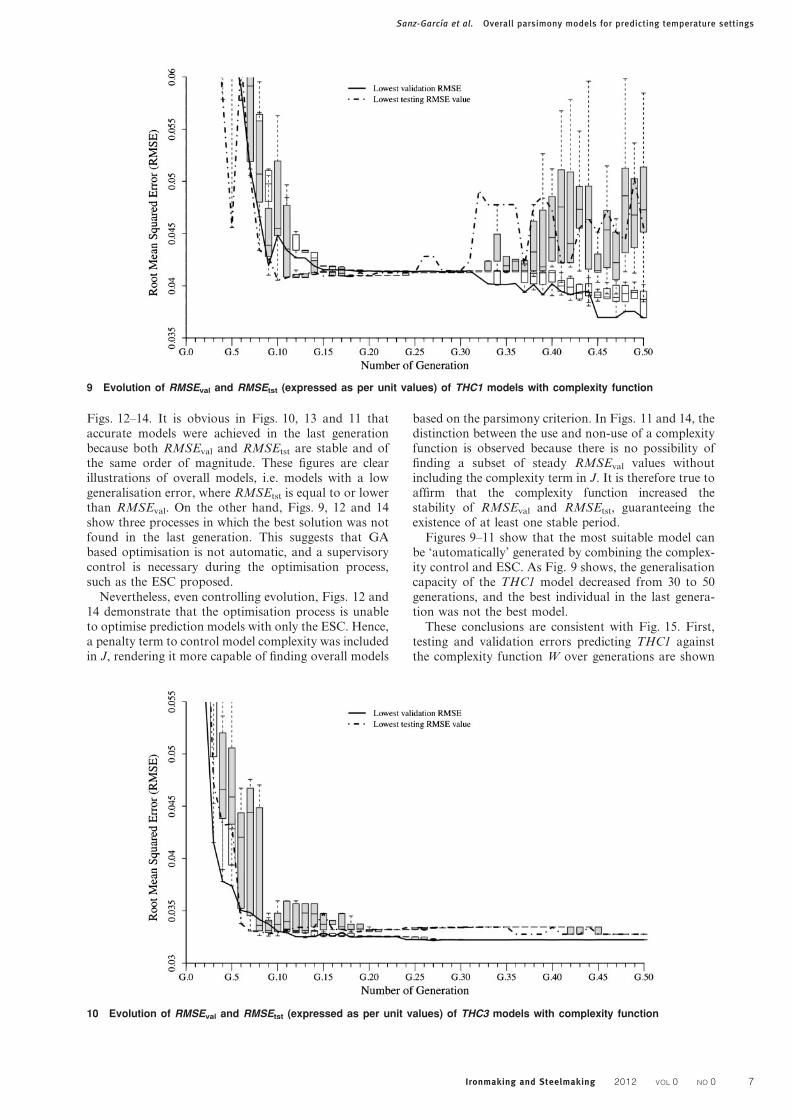
Figs. 12–14. It is obvious in Figs. 10, 13 and 11 thataccurate models were achieved in the last generationbecause both RMSEval and RMSEtst are stable and ofthe same order of magnitude. These figures are clearillustrations of overall models, i.e. models with a lowgeneralisation error, where RMSEtst is equal to or lowerthan RMSEval. On the other hand, Figs. 9, 12 and 14show three processes in which the best solution was notfound in the last generation. This suggests that GAbased optimisation is not automatic, and a supervisorycontrol is necessary during the optimisation process,such as the ESC proposed.
Nevertheless, even controlling evolution, Figs. 12 and14 demonstrate that the optimisation process is unableto optimise prediction models with only the ESC. Hence,a penalty term to control model complexity was includedin J, rendering it more capable of finding overall models
based on the parsimony criterion. In Figs. 11 and 14, thedistinction between the use and non-use of a complexityfunction is observed because there is no possibility offinding a subset of steady RMSEval values withoutincluding the complexity term in J. It is therefore true toaffirm that the complexity function increased thestability of RMSEval and RMSEtst, guaranteeing theexistence of at least one stable period.
Figures 9–11 show that the most suitable model canbe ‘automatically’ generated by combining the complex-ity control and ESC. As Fig. 9 shows, the generalisationcapacity of the THC1 model decreased from 30 to 50generations, and the best individual in the last genera-tion was not the best model.
These conclusions are consistent with Fig. 15. First,testing and validation errors predicting THC1 againstthe complexity function W over generations are shown
9 Evolution of RMSEval and RMSEtst (expressed as per unit values) of THC1 models with complexity function
10 Evolution of RMSEval and RMSEtst (expressed as per unit values) of THC3 models with complexity function
Sanz-Garcıa et al. Overall parsimony models for predicting temperature settings
Ironmaking and Steelmaking 2012 VOL 0 NO 0 7

in Fig. 15a and b with and without complexity control,respectively. The same is applied in the case of THC3with Fig. 15c and d and THC5 with Fig. 15e and f.Predicting THC1, the balance between RMSEval andRMSEtst is higher in Fig. 15a than in Fig. 15b becausethe penalty function reduced the number of overfittedmodels. As shown in Fig. 15b, the best model does nothave the lowest RMSEval, with the increase in RMSEtst
usually being directly dependent on W. In the case oftemperature THC3, Fig. 15d shows a lower density thanFig. 15c in the lower part of the plot, which means asharp reduction in computational cost. Finally, Fig. 15eand f confirm that if the GA cannot find the optimalsettings, the control of model complexity requires thedevelopment of less complex models (W between 5 and8).
Figure 8a and b shows the predictions of the THC5model against the measurements for the optimisation
method with and without the complexity penalty,respectively. In the case of THC1 and THC3, whichare not shown due to space constraints, the results weresimilar (see Supplementary Material) (SupplementaryMaterial). The prediction accuracy is higher usingcomplexity control, with absolute RMSEtst 10?8uC lowerthan RMSEtst and 13?6uC in the other case.
One disadvantage of GAs is the need for massive dataprocessing. As shown in Table 1, ESC based on CL mayreduce the total training computational cost. Using theproposed ESC,27 we have found that the performance ofthe resulting models does not decrease, while the totalcomputational costs are lower in two of the three casesstudied (Figs. 9–14). Figure 9 provides support forincluding a stopping criterion that significantly decreasesthe high risk of overfitting.
Table 2 reports the number and names of the totalselected inputs by GA based FS for each final model.
11 Evolution of RMSEval and RMSEtst (expressed as per unit values) of THC5 models with complexity function
12 Evolution of RMSEval and RMSEtst (expressed as per unit values) of THC1 models without complexity function
Sanz-Garcıa et al. Overall parsimony models for predicting temperature settings
8 Ironmaking and Steelmaking 2012 VOL 0 NO 0

13 Evolution of RMSEval and RMSEtst (expressed as per unit values) of THC3 models without complexity function
14 Evolution of RMSEval and RMSEtst (expressed as per unit values) of THC5 models without complexity function
Table 2 Selected inputs of best THC1, THC3 and THC5 models: bold type indicates attributes selected in all cases, anditalics in all cases except one
With Complexity Without Complexity
THC1 THC3 THC5 THC1 THC3 THC5
1 P Mn Mn C Mn Si2 ThickCoil Si Si Mn Si Cu3 TMPP2CNG S P Si V Ni4 VelMed ThickCoil Cr ThickCoil N B5 … WidthCoil B WidthCoil ThickCoil N6 … TMPP2CNG N TMPP2CNG WidthCoil ThickCoil7 … VelMed ThickCoil VelMed TMPP2CNG WidthCoil8 … … WidthCoil … VelMed TMPP2CNG9 … … TMPP2CNG … … VelMed10 … … VelMed … … …Total 4 7 10 7 8 9
Sanz-Garcıa et al. Overall parsimony models for predicting temperature settings
Ironmaking and Steelmaking 2012 VOL 0 NO 0 9

Figure 16 complements the information on the binaryselection array for THC1 prediction models, showingthe evolution of the different inputs selected for the tenbest individuals over 49 generations. Stopping genera-tion is represented using a triangle when the input wasnot finally selected and, conversely, an inverted triangle.
In previous research, Martınez-de-Pison et al.20
reported a substantial improvement, drastically reducing
the number of variables for the chemical composition ofsteel using principal component analysis (PCA).However, VelMed, TMPP1, WidthCoil, ThickCoil andTMPP2CNG were included in the models without priorsignificance rating. The disadvantage of PCA is that theinterpretation of the final models is more difficult as rawvariables are no longer being used. In this paper, FS hasbeen used to form a subset from all the variables without
15 Errors via aggregation coefficients W: THC1 a with complexity control and b without; THC3 c with complexity control
and d without; THC5 e with complexity control and f without. Black points represent validation and grey points are
testing data
Sanz-Garcıa et al. Overall parsimony models for predicting temperature settings
10 Ironmaking and Steelmaking 2012 VOL 0 NO 0
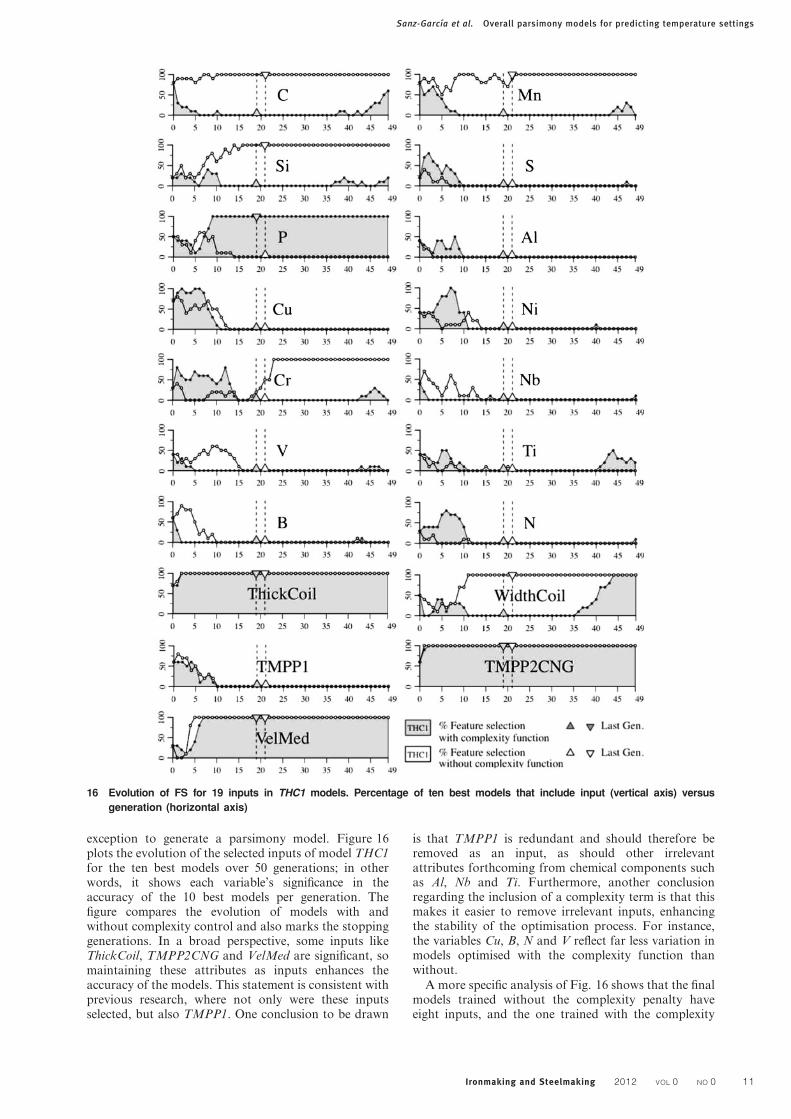
exception to generate a parsimony model. Figure 16plots the evolution of the selected inputs of model THC1for the ten best models over 50 generations; in otherwords, it shows each variable’s significance in theaccuracy of the 10 best models per generation. Thefigure compares the evolution of models with andwithout complexity control and also marks the stoppinggenerations. In a broad perspective, some inputs likeThickCoil, TMPP2CNG and VelMed are significant, somaintaining these attributes as inputs enhances theaccuracy of the models. This statement is consistent withprevious research, where not only were these inputsselected, but also TMPP1. One conclusion to be drawn
is that TMPP1 is redundant and should therefore beremoved as an input, as should other irrelevantattributes forthcoming from chemical components suchas Al, Nb and Ti. Furthermore, another conclusionregarding the inclusion of a complexity term is that thismakes it easier to remove irrelevant inputs, enhancingthe stability of the optimisation process. For instance,the variables Cu, B, N and V reflect far less variation inmodels optimised with the complexity function thanwithout.
A more specific analysis of Fig. 16 shows that the finalmodels trained without the complexity penalty haveeight inputs, and the one trained with the complexity
16 Evolution of FS for 19 inputs in THC1 models. Percentage of ten best models that include input (vertical axis) versus
generation (horizontal axis)
Sanz-Garcıa et al. Overall parsimony models for predicting temperature settings
Ironmaking and Steelmaking 2012 VOL 0 NO 0 11

control has only four inputs selected, which is the sameas saying we obtained half the complexity in the finalmodels with the proposed complexity control thanwithout. Both methods selected VelMed, ThickCoil andTMPP2CNG, but the method with complexity controlonly additionally chose attribute P, instead of thestandard method that added C, Si and Mn. In this case,and according to Guyon and Elisseeff,28 variables thatare useless by themselves can be useful together. C, Siand Mn have the same performance together as the firstmodel with only the variable P. This shows that bothfitness functions have the capacity to achieve highperformance models, but only our proposal generated aparsimony model. A similar behaviour was observedfor THC3 and THC5 prediction (see SupplementaryMaterial) (Supplementary Material).
ConclusionsThis paper reports the development of a methodologybased on data driven techniques for designing parsi-mony and overall models to predict CAF temperatureset points. For plant engineers, the main advantages arethe reduced complexity of the final models, bettergeneralisation capacity and computational time savedthat allow incorporating it into the CAF’s online controlsystem. The proposed methodology makes it easierfor plant engineers to deal with continuous productchanges, spending less time on adjusting models andreducing downtime costs.
Acknowledgements
The authors thank the European Union for its financialsupport through project no. RFS-PR-06035 and theAutonomous Government of La Rioja for its support inthe 3rd R&D&i Plan through project FOMENTA 2010/13.
References1. N. Yoshitani and A. Hasegawa: ‘Model-based control of strip
temperature for the heating furnace in continuous annealing’,
IEEE Trans. Control Syst. Technol., 1998, 6, (2), 146–156.
2. J.-S. Kim and J.-H. Chung: ‘Galvannealing behaviour of high strength
galvanized sheet steels’, Proc. Galvanised Steel Sheet Forum-
Automotive, London, UK, May 2000, IOM Communication Ltd.
103–108.
3. F. J. Martınez-de-Pison, A. Sanz, E. Martınez-de-Pison, E. Jimenez
and D. Conti: ‘Mining association rules from time series to explain
failures in a hot-dip galvanizing steel line’, Comput. Ind. Eng., 2012,
63, (1), 22–36.
4. J. Mahieu, M. De-Meyer and B. C. De-Cooman: ‘Galvanizability
of high strength steels for automotive applications’, Proc.
Galvanised Steel Sheet Forum-Automotive, London, UK, May
2000, IOM Communication Ltd. 185–198.
5. L. Bitschnau and M. Kozek: ‘Modeling and control of an industrial
continuous furnace’, Proc. Int. Conf. on ‘Computational intelli-
gence, modelling and simulation’, Brno, Czech, September 2009,
IEEE Computer Society, 231–236.
6. Z. Ming and Y. Datai: ‘A new strip temperature control method
for the heating section of continuous annealing line’, Proc. IEEE
Int. Conf. on ‘Cybernetics and intelligent systems’, Chengdu,
China, September 2008, IEEE Computer Society, 861–864.
7. F. T. P. de Medeiros, S. J. X. Noblat and A. M. F. Fileti: ‘Reviving
traditional blast furnace models with new mathematical approach’,
Ironmaking Steelmaking, 2007, 34, (5), 410–414.
8. D. M. Jones, J. Watton and K. J. Brown: ‘Comparison of hot
rolled steel mechanical property prediction models using linear
multiple regression, non-linear multiple regression and non-linear
artificial neural networks’, Ironmaking Steelmaking, 2005, 32, (5),
435–442.
9. M. Schlang and B. Lang: ‘Current and future development in
neural computation in steel processing’, Control Eng. Pract., 2001,
9, 975–986.
10. X. Wang, M. Yao and X. Chen: ‘Development of prediction
method for abnormalities in slab continuous casting using artificial
neural network models’, ISIJ Int., 2006, 46, (7), 1047–1053.
11. Y. I. Kim, K. C. Moon, B. S. Kang, C. Han and K. S. Chang:
‘Application of neural network to the supervisory control of a
reheating furnace in the steel industry’, Control Eng. Pract., 1998,
6, (8), 1009–1014.
12. M. Schlang, B. Feldkeller, B. Lang, T. Poppe and T. Runkler:
‘Neural computation in steel industry’, Proc. European Control
Conf. ‘99, Session BP-1, Karlsruhe, Germany, September 1999,
European Union Control Association, Session BP-1.
13. A. Agarwal, U. Tewary, F. Pettersson, S. Das, H. Saxen and N.
Chakraborti: ‘Analysing blast furnace data using evolutionary
neural network and multiobjective genetic algorithms’, Ironmaking
Steelmaking, 2010, 37, (5), 353–359.
14. P. J. Laitinen and H. Saxen: ‘A neural network based model of
sinter quality and sinter plant performance indices’, Ironmaking
Steelmaking, 2007, 34, (2), 109–114.
15. P. Tamminen, P. Ruha, J. I. Komi, T. Katajarinne, T. A. Kauppi,
J. P. Marttila and L. P. Karjalainen: ‘System for on/offline
prediction of mechanical properties and microstructural evolution
in hot rolled steel strip’, Ironmaking Steelmaking, 2007, 34, (2),
157–165.
16. Y.-Z. Lu and S. W. Markward: ‘Development and application of
an integrated neural system for an HDCL’, IEEE Trans. Neural
Networks, 1997, 8, (6), 1328–1337.
17. C. Schiefer, F. X. Rubenzucker, H. Peter Jorgl and H. R. Aberl: ‘A
neural network controls the galvannealing process’, IEEE Trans.
Ind. Appl., 1999, 35, (1), 114–118.
18. A. Pernıa-Espinoza, M. Castejon-Limas, A. Gonzalez-Marcos and
V. Lobato-Rubio: ‘Steel annealing furnace robust neural network
model’, Ironmaking Steelmaking, 2005, 32, (5), 418–426.
19. F. J. Martınez-De-Pison, F. Alba-Elıas, M. Castejon-Limas and J.
A. Gonzalez-Rodrıguez: ‘Improvement and optimisation of hot dip
galvanising line using neural networks and genetic algorithms’,
Ironmaking Steelmaking, 2006, 33, (4), 344–352.
20. F. J. Martınez-De-Pison, A. Pernıa, E. Jimenez-Macıas and R.
Fernandez: ‘Overall model of the dynamic behaviour of the steel
strip in an annealing heating furnace on a hot-dip galvanizing line’,
Revista de Metalurgia (Madrid), 2010, 46, (5), 405–420.
21. F. J. Martınez-De-Pison, L. Celorrio, M. Perez-De-La-Parte and
M. Castejon: ‘Optimising annealing process on hot dip galvanising
line based on robust predictive models adjusted with genetic
algorithms’, Ironmaking Steelmaking, 2011, 38, (3), 218–228.
22. E. Pal, A. Datta and S. Sahay: ‘An efficient model for batch
annealing using a neural network’, Mater. Manuf. Processes, 2006,
21, 556–561.
23. F. J. Martınez-De-Pison: ‘Optimizacion mediante tecnicas de
minerıa de datos del ciclo de recocido de una lınea de galvanizado’,
PhD thesis, University of La Rioja, Logrono, Spain, 2003.
24. S. C. Larson: ‘The shrinkage of the coefficient of multiple
correlation’, J. Educ. Psychol., 1931, 22, (1), 45–55.
25. RCore Team: ‘R: a language and environment for statistical
computing’; 2012, Vienna, R Foundation for Statistical
Computing.
26. M. Castejon-Limas, J. B. Ordieres Mere, E. P. Vergara, F. J.
Martınez-de-Pison, A. V. Pernıa and F. Alba: ‘The AMORE
package: A MORE flexible neural network package’, CRAN
Repository, 2009.
27. N. Morgan and H. Bourlard: ‘Generalization and parameter
estimation in feedforward nets: some experiments’, in ‘Advances in
neural information processing systems 2’, (ed. D. S. Touretzky),
630–637; 1990, San Francisco, CA, Morgan Kaufmann Publishers
Inc.
28. I. Guyon and A. Elisseeff: ‘An introduction to variable and feature
selection’, J. Mach. Learn. Res., 2003, 3, 1157–1182.
Sanz-Garcıa et al. Overall parsimony models for predicting temperature settings
12 Ironmaking and Steelmaking 2012 VOL 0 NO 0

Chapter 5
PUBLICATION III
Sanz-García, A., Antoñanzas-Torres, A., Fernández-Ceniceros, J. & Martínez-de-
Pisón, F. J. (2012). Overall models based on ensemble methods for predicting
continuous annealing furnace temperature settings, Ironmaking & Steelmaking,
available on line. DOI 10.1179/1743281213Y.0000000104.
The publisher and copyright holder corresponds to Maney Publishing, which is
the trading name of W.S.Maney & Son Ltd. The online version of this journal
are the URLs:
• http://maneypublishing.com/index.php/journals/irs/
• http://www.ingentaconnect.com/content/maney/ias
57

58 Chapter 5. PUBLICATION III
.........
58
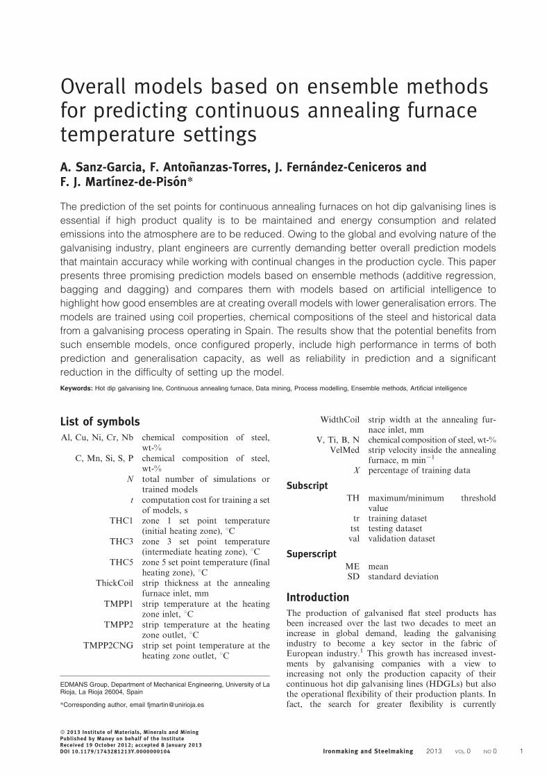
Overall models based on ensemble methodsfor predicting continuous annealing furnacetemperature settings
A. Sanz-Garcia, F. Antonanzas-Torres, J. Fernandez-Ceniceros andF. J. Martınez-de-Pison*
The prediction of the set points for continuous annealing furnaces on hot dip galvanising lines is
essential if high product quality is to be maintained and energy consumption and related
emissions into the atmosphere are to be reduced. Owing to the global and evolving nature of the
galvanising industry, plant engineers are currently demanding better overall prediction models
that maintain accuracy while working with continual changes in the production cycle. This paper
presents three promising prediction models based on ensemble methods (additive regression,
bagging and dagging) and compares them with models based on artificial intelligence to
highlight how good ensembles are at creating overall models with lower generalisation errors. The
models are trained using coil properties, chemical compositions of the steel and historical data
from a galvanising process operating in Spain. The results show that the potential benefits from
such ensemble models, once configured properly, include high performance in terms of both
prediction and generalisation capacity, as well as reliability in prediction and a significant
reduction in the difficulty of setting up the model.
Keywords: Hot dip galvanising line, Continuous annealing furnace, Data mining, Process modelling, Ensemble methods, Artificial intelligence
List of symbolsAl, Cu, Ni, Cr, Nb chemical composition of steel,
wt-%
C, Mn, Si, S, P chemical composition of steel,wt-%
N total number of simulations ortrained models
t computation cost for training a setof models, s
THC1 zone 1 set point temperature(initial heating zone), uC
THC3 zone 3 set point temperature(intermediate heating zone), uC
THC5 zone 5 set point temperature (finalheating zone), uC
ThickCoil strip thickness at the annealingfurnace inlet, mm
TMPP1 strip temperature at the heatingzone inlet, uC
TMPP2 strip temperature at the heatingzone outlet, uC
TMPP2CNG strip set point temperature at theheating zone outlet, uC
WidthCoil strip width at the annealing fur-nace inlet, mm
V, Ti, B, N chemical composition of steel, wt-%VelMed strip velocity inside the annealing
furnace, m min21
X percentage of training data
SubscriptTH maximum/minimum threshold
valuetr training dataset
tst testing datasetval validation dataset
SuperscriptME meanSD standard deviation
IntroductionThe production of galvanised flat steel products hasbeen increased over the last two decades to meet anincrease in global demand, leading the galvanisingindustry to become a key sector in the fabric ofEuropean industry.1 This growth has increased invest-ments by galvanising companies with a view toincreasing not only the production capacity of theircontinuous hot dip galvanising lines (HDGLs) but alsothe operational flexibility of their production plants. Infact, the search for greater flexibility is currently
EDMANS Group, Department of Mechanical Engineering, University of LaRioja, La Rioja 26004, Spain
*Corresponding author, email [email protected]
� 2013 Institute of Materials, Minerals and MiningPublished by Maney on behalf of the InstituteReceived 19 October 2012; accepted 8 January 2013DOI 10.1179/1743281213Y.0000000104 Ironmaking and Steelmaking 2013 VOL 0 NO 0 1

considered crucial in meeting the wide variety ofcustomer needs, especially given today’s rapidly evolvingmarkets such as vehicle manufacturing.2 The strategy isclear: the more different products are supplied, the morenew markets will be open up. However, this requiredflexibility may also generate significant problems such asidle times in the continuous mode of operation orreduction in the quality of coatings. Therefore, HDGLplant engineers need to make multiple adjustments whendealing with new products until the right adherence anduniformity in coating are achieved. Reducing the timeneeded to determine optimal set points is also crucial forsaving costs.3
This paper focuses on enhancing the accuracy andefficiency with which the operating set points arecalculated for a continuous annealing furnace (CAF)on an HDGL. Over the last few decades, manymathematical models based on heat and mass balancehave been developed to predict furnace temperaturesettings.4 However, those models have some disadvan-tages such as clear difficulties in tuning model para-meters to new product specifications, strong dependenceon the experience of the engineer and long computationtime to modify models. Recent papers have proved thatdata driven models based on artificial intelligence (AI)are a good alternative for developing accurate predictionmodels in the steel industry.5 To take advantage of thesetechniques in the modelling of the galvanising process,the main requirements are the availability of historicaldata, detailed knowledge of the chemical composition ofsteel and time to train the models.
We propose the use of models based on ensemblemethods (EMs) with high overall performance inpredicting system set points.6 The major problem ofthe aforementioned AI based models is that they do notmaintain consistent prediction accuracy with all types ofproducts, especially with products not previouslyprocessed. Unlike single AI based models, EMs arebuilt using a set of models and the final output is acombination of the outputs of each individual model.7
Ensemble methods (EMs) have the same requirements assingle models, but two independent studies have shownthat combining outputs from multiple predictorsincrease their generalisation capacity.8,9 This may makeEMs very attractive for working in rapidly changingenvironments.10
In this paper, three EMs, i.e. additive regression11
(AR), bootstrap aggregating6 (bagging) and dagging,12
are developed to adjust CAF temperature settings in anHDGL. Additionally, five data driven models, i.e. leastmedian squared linear regression13 (LMSQ), linearregression14 (LR), Quinlan’s improved M5 algorithm15
(M5P), multilayer perceptron neural network16 (MLP)and support vector machine17 (SVM), are chosen fromliterature as basic components of the ensembles. Acomparative evaluation procedure is also included tohelp plant engineers select the best performing model.The results for furnace temperature set point predictionsobtained with this method highlight the benefits of usingEMs rather than other data driven models for thedevelopment of better overall models. Primarily, theirhigher generalisation capacity reduces the need forcontinual tuning of model parameters when dealing withnew products. The additional ease with which models canbe set up is the other crucial advantage for engineers.
In short, EMs have the capacity to provide highperformance prediction models for online furnacecontrol systems, leading to very low levels of divergencebetween the ideal annealing profile and the striptemperature actually measured.
Description of problemA continuous HDGL is a well known industrial processcomposed of several independent sections, each oneinvolving a specific treatment.18 The heart of theannealing treatment is the CAF, which is divided up asfollows: preheating area, heating and holding area, slowcooling area, jet cooling area and overaging area. Insidethe CAF, the strip is recrystallised by heating it up andholding it at temperatures of between 750 and 850uC;then, the strip is cooled down at different rates to theliquid zinc bath temperature of between 450 and 470uC.In practice, full adjustment to the annealing profileprescribed can be only guaranteed by feeding the stripinto the CAF at a constant speed.19 For that reason, thecontrol of CAF temperature settings is crucial forproper heating along the steel strip and consequently,has significant influence on the mechanical properties ofthe steel and the quality of the coating adherence.20–23
In this study, the CAF’s online control systemincludes models for estimating three furnace tempera-ture set points. These predictions represent a complextask, mainly due to continuous variations in productspecifications and in the chemical composition of thesteel used. The current data based models tend tospecialise in specific groups of coils and do not maintaintheir accuracy with products not previously processed.24,25
Several different models therefore need to be developedand tested to solve this problem, but this task may takeup enormous amounts of time and effort. The challengestill lies in developing better overall prediction modelscapable of working out CAF temperature settings fornew coils and different operating conditions whilemaintaining accuracy with no additional model trainingphases.
Related researchThe prediction of CAF temperature settings is anunresolved challenge for enhancing the online controlof the annealing process.1 Classical approaches deter-mine temperatures empirically on the basis of a numberof process trials that generate prediction models using aset of tables.26 This method is not efficient because thereare high costs associated with in plant trials. The mostwidely used alternative is to develop mathematicalmodels that consider both thermodynamic propertiesand heat transfer mechanics inside the CAF.17,27–31
However, as Prieto et al.32 claim, some furnacecharacteristics and material properties may changeappreciably with different compositions and heat treat-ment of steel, and this may influence these modelssignificantly. This happens, for instance, with the specificheat capacity of the strip and heating power of burners.So more than just metallurgical knowledge is requiredto determine precise CAF settings for each coil.23
Developing models that are based on data may improveprediction capacity because they take into account notonly the inherent non-linearities of the annealing processbut also the knowhow of plant operators and historical
Sanz-Garcia et al. Predicting continuous annealing furnace temperature settings
2 Ironmaking and Steelmaking 2013 VOL 0 NO 0

data.33,34 Since 1998, several authors have reported onstudies related to regression models that use historicaldata from steel processes.20,35 In recent years, interest insuch models has grown, especially in those based onartificial neural networks (ANNs),2 genetic algorithmguided neural network (GA-NN) ensemble models,36
fuzzy logic models,37 fuzzy ANNs,38 Bayesian models39
and Gaussian mixture models.40 For instance, severalapplications have been developed applying fuzzy settheory in HDGL for system control and qualitymanagement. Kuru and Kuru proposed a new galvan-nealing control system based on a fuzzy inference systemthat contributed to a significant improvement in theuniformity and quality of the coating layer running atlower limit of permissible coating values.41 Recently,Zhang et al. proposed a feedforward control methodbased on fuzzy adaptive model for the thickness controlprocess of galvanising coating.42
Likewise, ANNs have been successfully applied inmany parts of the galvanising process. Schiefer et al.43
report a combination of clustering and RBFN toimprove the predictor of an online galvannealing processcontrol. Lu and Markward44 reduce the coating weighttransitional footage by integrating ANN with thecoating weight control system in an HDGL. A 2005paper by Pernıa-Espinoza et al.45 shows the highperformance of robust MLP estimating the velocity setpoint of coils inside the CAF using only theircharacteristics and furnace temperatures. Conversely,Martınez-de-Pison et al.46 develop similar MLPs topredict CAF temperature set points but without varyingstrip velocity.
Finally, the problem of finding optimal ANNs hasbecome more tractable with the advent of geneticalgorithms,47 since which time several models have beenreported with better balances between accuracy andcomplexity in predicting the optimal settings of theannealing process in an HDGL48 and estimating thestrip temperature during the annealing treatment insidethe CAF.49
Lastly, Koksal et al. and Liao et al. presented acomplete revision of most relevant data mining techni-ques developed during the past decade and theirapplications in steel and manufacturing industry.50,51
MethodologyMany techniques for handling regression tasks havebeen proposed in literature, but even today, designingautomatic methodologies that choose the best perform-ing model for a particular application remains achallenge. One current proposal is based on selectingnot only the most accurate model for predicting withstored data but also the model with the highestgeneralisation capacity. In the following section, themethodology proposed is described on the basis of acomparative evaluation to search for the models withthe best balance between accuracy, generalisationcapacity and computation cost during the trainingphase.
Overview of modelsEnsemble learning is a paradigm of ML where multiplesingle models, referred to as base learners (BLs), arefitted and combined to give a better solution to aparticular problem. An EM constructs a set of
predictors and then combines their outputs to obtainan improved single response (see Fig. 1). Specifically, thefinal output of an EM is the average or weighted averagein regression tasks. Two main conditions need to beaddressed for improved results to be achieved: highaccuracy in all individual models and diversity betweentheir predictions. A brief description of the EMs selectedfollows:
(i) additive regression (AR) is a metamodel thatenhances the performance of a regression basemodel. Each iteration fits a model to theresiduals left by the predictor on the previousiteration. The output is obtained by addingtogether the predictions of all the models. Themain parameter is the shrinkage or learning rate,which helps prevent overfitting and has asmoothing effect but increases the learningtime11
(ii) bootstrap aggregating (bagging) is a metamodelthat averages a number of BLs fitted with a set ofdifferent training datasets. These datasets aregenerated by sampling uniformly and withreplacement of the original data (bootstrapping)6
(iii) dagging is a technique similar to bagging but inwhich the training datasets are created usingdisjoint samples. A number of disjoint, stratifiedfolds out of the data are generated to train a BLwith each subset. Dagging is potentially verysuitable for BLs that are quadratic (or evenworse in terms of time consumption) regardingthe lowest number of instances in each trainingdataset.12
The best performing BLs then need to be selected on thebasis of the support provided by previous studies.52 Fivealgorithms are finally selected here from an initial list ofseven, as follows:
(i) least median squared linear regression is arobust linear regression model based on classi-cal least squares regression that minimises themedian of the squared residuals. Its majordisadvantage is its lack of efficiency because ofits slow convergence rate13
(ii) linear regression is an improved version of atraditional scheme for linear predictions thatincludes the Akaike criterion53 for featureselection and can also deal with weightedinstances14
(iii) M5P tree (M5P) is an improvement of theoriginal Quinlan’s M5 algorithm for regressiontasks by generating a decision tree with simpleLR models at its leaves15,54
1 Basic layout of EMs by averaging a set of numerical
inputs
Sanz-Garcia et al. Predicting continuous annealing furnace temperature settings
Ironmaking and Steelmaking 2013 VOL 0 NO 0 3
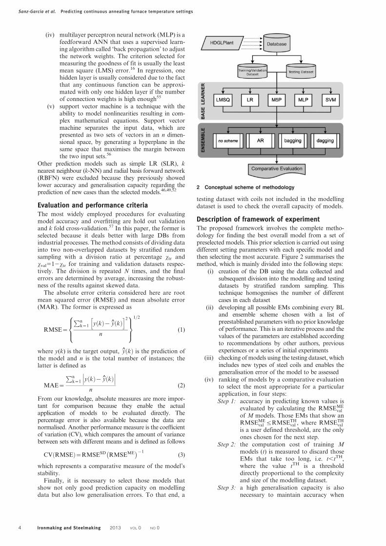
(iv) multilayer perceptron neural network (MLP) is afeedforward ANN that uses a supervised learn-ing algorithm called ‘back propagation’ to adjustthe network weights. The criterion selected formeasuring the goodness of fit is usually the leastmean square (LMS) error.16 In regression, onehidden layer is usually considered due to the factthat any continuous function can be approxi-mated with only one hidden layer if the numberof connection weights is high enough55
(v) support vector machine is a technique with theability to model nonlinearities resulting in com-plex mathematical equations. Support vectormachine separates the input data, which arepresented as two sets of vectors in an n dimen-sional space, by generating a hyperplane in thesame space that maximises the margin betweenthe two input sets.56
Other prediction models such as simple LR (SLR), knearest neighbour (k-NN) and radial basis forward network(RBFN) were excluded because they previously showedlower accuracy and generalisation capacity regarding theprediction of new cases than the selected models.46,49,52
Evaluation and performance criteriaThe most widely employed procedures for evaluatingmodel accuracy and overfitting are hold out validationand k fold cross-validation.57 In this paper, the former isselected because it deals better with large DBs fromindustrial processes. The method consists of dividing datainto two non-overlapped datasets by stratified randomsampling with a division ratio at percentage xtr andxval512xtr for training and validation datasets respec-tively. The division is repeated N times, and the finalerrors are determined by average, increasing the robust-ness of the results against skewed data.
The absolute error criteria considered here are rootmean squared error (RMSE) and mean absolute error(MAR). The former is expressed as
RMSE~
Pnk~1 y kð Þ{ y kð Þ
h i2
n
8><>:
9>=>;
1=2
(1)
where y(k) is the target output, y kð Þ is the prediction ofthe model and n is the total number of instances; thelatter is defined as
MAE~
Pnk~1 y kð Þ{ y kð Þ
��� ���n
(2)
From our knowledge, absolute measures are more impor-tant for comparison because they enable the actualapplication of models to be evaluated directly. Thepercentage error is also available because the data arenormalised. Another performance measure is the coefficientof variation (CV), which compares the amount of variancebetween sets with different means and is defined as follows
CV RMSEð Þ~RMSESD RMSEME� �{1
(3)
which represents a comparative measure of the model’sstability.
Finally, it is necessary to select those models thatshow not only good prediction capacity on modellingdata but also low generalisation errors. To that end, a
testing dataset with coils not included in the modellingdataset is used to check the overall capacity of models.
Description of framework of experimentThe proposed framework involves the complete metho-dology for finding the best overall model from a set ofpreselected models. This prior selection is carried out usingdifferent setting parameters with each specific model andthen selecting the most accurate. Figure 2 summarises themethod, which is mainly divided into the following steps:
(i) creation of the DB using the data collected andsubsequent division into the modelling and testingdatasets by stratified random sampling. Thistechnique homogenises the number of differentcases in each dataset
(ii) developing all possible EMs combining every BLand ensemble scheme chosen with a list ofpreestablished parameters with no prior knowledgeof performance. This is an iterative process and thevalues of the parameters are established accordingto recommendations by other authors, previousexperiences or a series of initial experiments
(iii) checking of models using the testing dataset, whichincludes new types of steel coils and enables thegeneralisation error of the model to be assessed
(iv) ranking of models by a comparative evaluationto select the most appropriate for a particularapplication, in four steps:
Step 1: accuracy in predicting known values isevaluated by calculating the RMSEME
val
of M models. Those EMs that show anRMSEME
val ƒRMSETHval , where RMSETH
val
is a user defined threshold, are the onlyones chosen for the next step.
Step 2: the computation cost of training Mmodels (t) is measured to discard thoseEMs that take too long, i.e. t,tTH,where the value tTH is a thresholddirectly proportional to the complexityand size of the modelling dataset.
Step 3: a high generalisation capacity is alsonecessary to maintain accuracy when
2 Conceptual scheme of methodology
Sanz-Garcia et al. Predicting continuous annealing furnace temperature settings
4 Ironmaking and Steelmaking 2013 VOL 0 NO 0
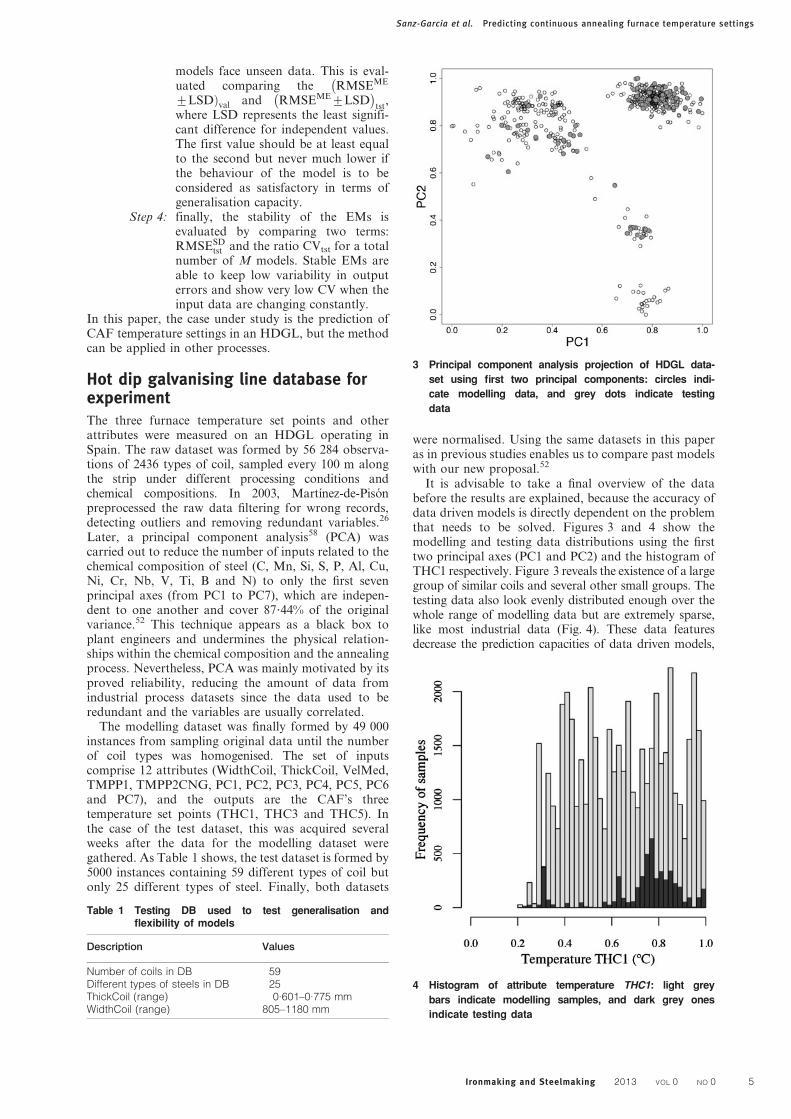
models face unseen data. This is eval-uated comparing the RMSEME
�+LSDÞval and RMSEME+LSD
� �tst
,where LSD represents the least signifi-cant difference for independent values.The first value should be at least equalto the second but never much lower ifthe behaviour of the model is to beconsidered as satisfactory in terms ofgeneralisation capacity.
Step 4: finally, the stability of the EMs isevaluated by comparing two terms:RMSESD
tst and the ratio CVtst for a totalnumber of M models. Stable EMs areable to keep low variability in outputerrors and show very low CV when theinput data are changing constantly.
In this paper, the case under study is the prediction ofCAF temperature settings in an HDGL, but the methodcan be applied in other processes.
Hot dip galvanising line database forexperimentThe three furnace temperature set points and otherattributes were measured on an HDGL operating inSpain. The raw dataset was formed by 56 284 observa-tions of 2436 types of coil, sampled every 100 m alongthe strip under different processing conditions andchemical compositions. In 2003, Martınez-de-Pisonpreprocessed the raw data filtering for wrong records,detecting outliers and removing redundant variables.26
Later, a principal component analysis58 (PCA) wascarried out to reduce the number of inputs related to thechemical composition of steel (C, Mn, Si, S, P, Al, Cu,Ni, Cr, Nb, V, Ti, B and N) to only the first sevenprincipal axes (from PC1 to PC7), which are indepen-dent to one another and cover 87?44% of the originalvariance.52 This technique appears as a black box toplant engineers and undermines the physical relation-ships within the chemical composition and the annealingprocess. Nevertheless, PCA was mainly motivated by itsproved reliability, reducing the amount of data fromindustrial process datasets since the data used to beredundant and the variables are usually correlated.
The modelling dataset was finally formed by 49 000instances from sampling original data until the numberof coil types was homogenised. The set of inputscomprise 12 attributes (WidthCoil, ThickCoil, VelMed,TMPP1, TMPP2CNG, PC1, PC2, PC3, PC4, PC5, PC6and PC7), and the outputs are the CAF’s threetemperature set points (THC1, THC3 and THC5). Inthe case of the test dataset, this was acquired severalweeks after the data for the modelling dataset weregathered. As Table 1 shows, the test dataset is formed by5000 instances containing 59 different types of coil butonly 25 different types of steel. Finally, both datasets
were normalised. Using the same datasets in this paperas in previous studies enables us to compare past modelswith our new proposal.52
It is advisable to take a final overview of the databefore the results are explained, because the accuracy ofdata driven models is directly dependent on the problemthat needs to be solved. Figures 3 and 4 show themodelling and testing data distributions using the firsttwo principal axes (PC1 and PC2) and the histogram ofTHC1 respectively. Figure 3 reveals the existence of a largegroup of similar coils and several other small groups. Thetesting data also look evenly distributed enough over thewhole range of modelling data but are extremely sparse,like most industrial data (Fig. 4). These data featuresdecrease the prediction capacities of data driven models,
Table 1 Testing DB used to test generalisation andflexibility of models
Description Values
Number of coils in DB 59Different types of steels in DB 25ThickCoil (range) 0.601–0.775 mmWidthCoil (range) 805–1180 mm
3 Principal component analysis projection of HDGL data-
set using first two principal components: circles indi-
cate modelling data, and grey dots indicate testing
data
4 Histogram of attribute temperature THC1: light grey
bars indicate modelling samples, and dark grey ones
indicate testing data
Sanz-Garcia et al. Predicting continuous annealing furnace temperature settings
Ironmaking and Steelmaking 2013 VOL 0 NO 0 5

but the article shows that our proposed EMs are a betterway of dealing with these problems than single models.
Results and discussionIn this paper, we mainly analyse three types of EM to predictthe temperature set points (THC1, THC3 and THC5) for aCAF on an HDGL. However, the results concerning THC1are only reported to summarise the information, due to thefact that the results from training the THC3 and THC5prediction models are similar to the first one.
The performance of models predicting THC1 is evaluatedfollowing the steps and criteria of the proposed methodol-ogy. These evaluations are carried out with the statisticalsoftware R-project 2?1159 running on a dual quadcoreOpteron server with Linux SUSE 11?2. Additionally, themodels are implemented using the WEKA workbench60
and R-project packages AMORE61 and RWeka.62
The ranges of the values of the setting parameters usedto generate models with different configurations are listedin Table 2 for BLs and Table 3 for EMs. Validation andtesting simulations were repeated N510 times for eachparticular configuration, selecting only the best case foreach algorithm. Table 4 presents the mean and standarddeviation of both error measures (RMSE and MAE) forthe best models and also the total computation time to setup a number of M510 models with the same settingparameters. Likewise, Table 5 shows the results reportedby Martınez-de-Pison et al.52 from earlier research intoMLP models. These results allow us to discuss theadvantages and disadvantages by comparing the two
Table 2 Parameter specifications for BLs
Algorithm Parameter Values
LR Ridge 0.1, 0.3, …, 4Attribute selection Greedy
LSMQ Sample size 4, 8, …, 400M5P Min. instances/leaf 2, 4, …, 80
Prune TrueUnsmoothed model False
MLP Learning rate 0.1, 0.2, …, 0.8Momentum 0.1, 0.2, …, 0.6Num. iterations 50 000–10 000Num. hidden neurons 3, 5, 7, …, 40Decay learning rate TrueAutoreset network TrueValidation set size 20%Validation threshold 15, 25, …, 55
SVM C 1.0E 1.0E212e parameter 0.001Tolerance 0.001Kernel type PolynomialPoly. exponent 1, 1.02, …, 2.50
Table 3 Parameter specifications for ensemble schemes
Scheme Parameter Values
AR Shrinkage 0.2, 0.3, …, 1Num. iterations 10, 20, …, 80
Bagging Subset size 10, 20, …, 100Num. learning rounds 15, 20, …, 80
Dagging Num. folds 2, 3, …, 15
Table 4 Results of modelling process for THC1 prediction models (sorted by RMSEMEval )
Training error Validation error
Algorithm RMSEMEtr RMSESD
tr MAEMEtr MAESD
tr RMSEMEval RMSESD
val MAEMEval MAESD
val t/s
AR M5P 0.0124 0.0003 0.0065 0.0001 0.0148 0.0009 0.0071 0.0002 1799Bg M5P 0.0148 0.0001 0.0079 0.0001 0.0166 0.0008 0.0084 0.0002 3492Dg M5P 0.0176 0.0003 0.0096 0.0002 0.0189 0.0014 0.0100 0.0002 117Bg SVM 0.0315 0.0001 0.0194 0.0001 0.0314 0.0003 0.0195 0.0001 396 000AR MLP 0.0339 0.0003 0.0237 0.0003 0.0336 0.0004 0.0236 0.0002 4000Dg SVM 0.0336 0.0002 0.0218 0.0001 0.0337 0.0004 0.0218 0.0002 93 000Bg MLP 0.0376 0.0003 0.0263 0.0002 0.0378 0.0008 0.0263 0.0004 20 000Dg MLP 0.0382 0.0003 0.0268 0.0002 0.0380 0.0004 0.0267 0.0002 6243AR LR 0.0477 0.0003 0.0351 0.0001 0.0473 0.0007 0.0349 0.0003 194AR LMSQ 0.0481 0.0001 0.0350 0.0001 0.0475 0.0001 0.0348 0.0001 33 156Bg LR 0.0475 0.0002 0.0350 0.0001 0.0476 0.0005 0.0350 0.0002 151Bg LMSQ 0.0484 0.0002 0.0349 0.0001 0.0476 0.0005 0.0342 0.0002 94 949Dg LR 0.0475 0.0002 0.0350 0.0001 0.0478 0.0005 0.0352 0.0003 17Dg LMSQ 0.0482 0.0003 0.0351 0.0001 0.0484 0.0005 0.0351 0.0002 1357AR SVM 0.0510 0.0003 0.0413 0.0001 0.0511 0.0006 0.0419 0.0002 8608
Table 5 Results of modelling process of MLP models predicting for THC1 (sorted by RMSEMEval ) (source: Martınez-de-
Pison et al.52)
Training errors Validation errors
Algorithm RMSEMEtr RMSESD
tr MAEMEtr MAESD
tr RMSEMEval RMSESD
val MAESDval MAEME
val t/s
MLP h540 0.0303 0.0020 0.0211 0.0021 0.0305 0.0020 0.0212 0.0022 52 167MLP h510 0.0308 0.0008 0.0209 0.0008 0.0309 0.0009 0.0210 0.0008 9958MLP h535 0.0306 0.0029 0.0213 0.0031 0.0311 0.0033 0.0214 0.0032 34 582MLP h507 0.0313 0.0004 0.0216 0.0006 0.0317 0.0007 0.0217 0.0006 9932MLP h505 0.0325 0.0004 0.0225 0.0003 0.0328 0.0007 0.0226 0.0003 7401MLP h503 0.0355 0.0005 0.0252 0.0003 0.0356 0.0005 0.0252 0.0004 3643
Sanz-Garcia et al. Predicting continuous annealing furnace temperature settings
6 Ironmaking and Steelmaking 2013 VOL 0 NO 0
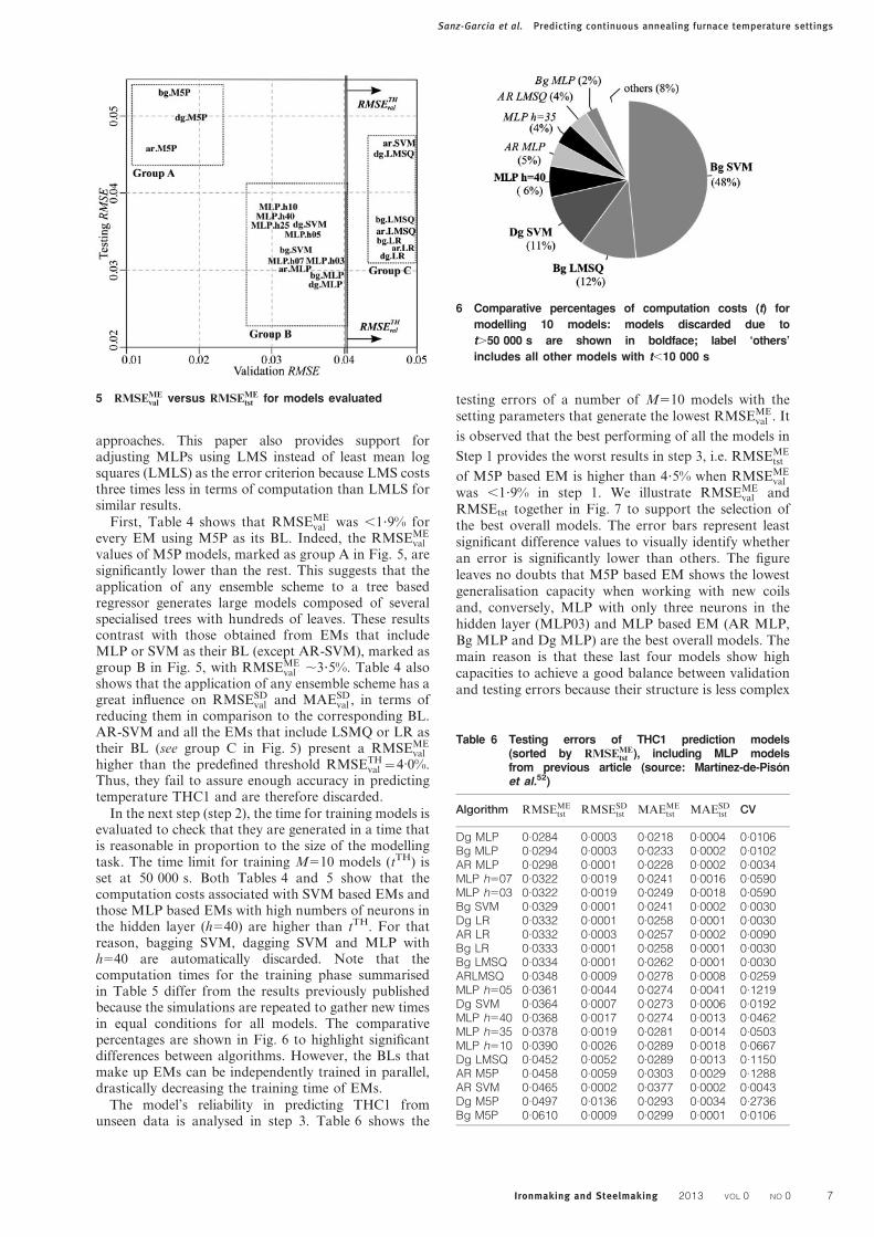
approaches. This paper also provides support foradjusting MLPs using LMS instead of least mean logsquares (LMLS) as the error criterion because LMS coststhree times less in terms of computation than LMLS forsimilar results.
First, Table 4 shows that RMSEMEval was ,1?9% for
every EM using M5P as its BL. Indeed, the RMSEMEval
values of M5P models, marked as group A in Fig. 5, aresignificantly lower than the rest. This suggests that theapplication of any ensemble scheme to a tree basedregressor generates large models composed of severalspecialised trees with hundreds of leaves. These resultscontrast with those obtained from EMs that includeMLP or SVM as their BL (except AR-SVM), marked asgroup B in Fig. 5, with RMSEME
val ,3?5%. Table 4 alsoshows that the application of any ensemble scheme has agreat influence on RMSESD
val and MAESDval , in terms of
reducing them in comparison to the corresponding BL.AR-SVM and all the EMs that include LSMQ or LR astheir BL (see group C in Fig. 5) present a RMSEME
val
higher than the predefined threshold RMSETHval ~4:0%.
Thus, they fail to assure enough accuracy in predictingtemperature THC1 and are therefore discarded.
In the next step (step 2), the time for training models isevaluated to check that they are generated in a time thatis reasonable in proportion to the size of the modellingtask. The time limit for training M510 models (tTH) isset at 50 000 s. Both Tables 4 and 5 show that thecomputation costs associated with SVM based EMs andthose MLP based EMs with high numbers of neurons inthe hidden layer (h540) are higher than tTH. For thatreason, bagging SVM, dagging SVM and MLP withh540 are automatically discarded. Note that thecomputation times for the training phase summarisedin Table 5 differ from the results previously publishedbecause the simulations are repeated to gather new timesin equal conditions for all models. The comparativepercentages are shown in Fig. 6 to highlight significantdifferences between algorithms. However, the BLs thatmake up EMs can be independently trained in parallel,drastically decreasing the training time of EMs.
The model’s reliability in predicting THC1 fromunseen data is analysed in step 3. Table 6 shows the
testing errors of a number of M510 models with thesetting parameters that generate the lowest RMSEME
val . It
is observed that the best performing of all the models in
Step 1 provides the worst results in step 3, i.e. RMSEMEtst
of M5P based EM is higher than 4?5% when RMSEMEval
was ,1?9% in step 1. We illustrate RMSEMEval and
RMSEtst together in Fig. 7 to support the selection ofthe best overall models. The error bars represent leastsignificant difference values to visually identify whetheran error is significantly lower than others. The figureleaves no doubts that M5P based EM shows the lowestgeneralisation capacity when working with new coilsand, conversely, MLP with only three neurons in thehidden layer (MLP03) and MLP based EM (AR MLP,Bg MLP and Dg MLP) are the best overall models. Themain reason is that these last four models show highcapacities to achieve a good balance between validationand testing errors because their structure is less complex
5 RMSEMEval versus RMSEME
tst for models evaluated
6 Comparative percentages of computation costs (t) for
modelling 10 models: models discarded due to
t.50 000 s are shown in boldface; label ‘others’
includes all other models with t,10 000 s
Table 6 Testing errors of THC1 prediction models(sorted by RMSEME
tst ), including MLP modelsfrom previous article (source: Martınez-de-Pisonet al.52)
Algorithm RMSEMEtst RMSESD
tst MAEMEtst MAESD
tst CV
Dg MLP 0.0284 0.0003 0.0218 0.0004 0.0106Bg MLP 0.0294 0.0003 0.0233 0.0002 0.0102AR MLP 0.0298 0.0001 0.0228 0.0002 0.0034MLP h507 0.0322 0.0019 0.0241 0.0016 0.0590MLP h503 0.0322 0.0019 0.0249 0.0018 0.0590Bg SVM 0.0329 0.0001 0.0241 0.0002 0.0030Dg LR 0.0332 0.0001 0.0258 0.0001 0.0030AR LR 0.0332 0.0003 0.0257 0.0002 0.0090Bg LR 0.0333 0.0001 0.0258 0.0001 0.0030Bg LMSQ 0.0334 0.0001 0.0262 0.0001 0.0030ARLMSQ 0.0348 0.0009 0.0278 0.0008 0.0259MLP h505 0.0361 0.0044 0.0274 0.0041 0.1219Dg SVM 0.0364 0.0007 0.0273 0.0006 0.0192MLP h540 0.0368 0.0017 0.0274 0.0013 0.0462MLP h535 0.0378 0.0019 0.0281 0.0014 0.0503MLP h510 0.0390 0.0026 0.0289 0.0018 0.0667Dg LMSQ 0.0452 0.0052 0.0289 0.0013 0.1150AR M5P 0.0458 0.0059 0.0303 0.0029 0.1288AR SVM 0.0465 0.0002 0.0377 0.0002 0.0043Dg M5P 0.0497 0.0136 0.0293 0.0034 0.2736Bg M5P 0.0610 0.0009 0.0299 0.0001 0.0106
Sanz-Garcia et al. Predicting continuous annealing furnace temperature settings
Ironmaking and Steelmaking 2013 VOL 0 NO 0 7

and not so specialised in coils already treated. Moreover,some models sometimes present lower RMSEME
tst thanRMSEME
val because the validation dataset may be morecomplex than testing dataset.
Finally, the stability of models is measured andcompared by determining the RMSESD
tst and CVtst.Stability is formally defined as the degree to which atechnique creates repeatable results, given differentdatasets sampled from the same data. The aim is tofind those models that have the lowest RMSESD
tst andCVtst at the same time. Models are not very reliable ifthey predict different values each time there are slightchanges in the input data or even in some of the settingparameters of the model itself. Table 6 shows that EMsthat use MLP as BL are the more stable because their
CVtst are at least four times lower than each single MLP.Additionally, Fig. 8 lends support to previous observa-tions by illustrating RMSEtst as a box plot of the testingerror distribution. It can be claimed that EMs usingMLP as BL have a narrower RMSEtst distribution thanany single data driven model.
ConclusionsThis paper mainly presents three ensemble schemes thatcombine the outputs of several data driven models topredict temperature set points for a CAF on an HDGL.The main contributions relate to the description of amethodology for evaluating models, the comparativeevaluation of 15 cases and the final recommendations
7 Bar plot with error bars of RMSEMEval and RMSEME
tst : dark and light grey bars correspond to validation and testing errors
respectively; error bars represent least significant difference between means; thus, two overlapping bars indicate non-
significant difference and non-overlapping bars indicate opposite
8 Box plots of RMSE (left, validation; right, testing): whiskers cover those samples that are outside interquartile range
but are not outliers; crosses represent outliers that are samples at distance of .1?5 times interquartile range; grey
dots and grey lines are mean and median of data respectively
Sanz-Garcia et al. Predicting continuous annealing furnace temperature settings
8 Ironmaking and Steelmaking 2013 VOL 0 NO 0

for using ensemble learning as a regression technique.Ensemble methods generally show themselves to behighly efficient and reliable in terms of computationcost, generalisation capacity and ease of determinationof the best model configuration. However, comparativeevaluation proves that the use of MLP as BL is the bestchoice for generating the best performing model, i.e. ARMLP, Bg MLP and Dg MLP. Compared to single MLP,MLP based EM achieves similar accuracy in predictingtemperature set points for types of coils stored in themodelling DB but a lower generalisation error with coilsnot previously processed. This demonstrates that EMsare universal in nature and better suited for workingwith low quality and sparse DBs from industrialprocesses. Finally, the extra cost in computation timerequired for these models is not so restrictive if it isconsidered that they can be easily parallelised and plantengineers can also avoid continually having to changethe model for new products thanks to its higher overallcapacity and stability.
Acknowledgements
The authors are grateful for financial support providedby the European Union via project no. RFS-PR-06035,by the University of La Rioja via grant FPI-2012 and forsupport provided by the Autonomous Government ofLa Rioja under its 3er Plan Riojano de IzDzI viaproject FOMENTA 2010/13.
References1. M. M. Prieto, F. J. Fernandez and J. L. Rendueles: ‘Thermal
performance of annealing line heating furnace’, Ironmaking
Steelmaking, 2005, 32, (2), 171–176.
2. M. Schlang and B. Lang: ‘Current and future development in
neural computation in steel processing’, Control Eng. Pract., 2001,
9, 975–986.
3. J. B. Ordieres, A. Gonzalez, J. A. Gonzalez and V. Lobato:
‘Estimation of mechanical properties of steel strip in hot dip
galvanising lines’, Ironmaking Steelmaking, 2004, 31, (1), 43–50.
4. F. T. P. de Medeiros, S. J. X. Noblat and A. M. F. Fileti: ‘Reviving
traditional blast furnace models with new mathematical approach’,
Ironmaking Steelmaking, 2007, 34, (5), 410–414.
5. P. J. Laitinen and H. Saxen: ‘A neural network based model of
sinter quality and sinter plant performance indices’, Ironmaking
Steelmaking, 2007, 34, (2), 109–114.
6. L. Breiman: ‘Bagging predictors’, Mach. Learn., 1996, 24, (2), 123–
140.
7. Z. Zhou: ‘Encyclopedia of database systems’; 2009, Berlin,
Springer.
8. E. Bauer and R. Kohavi: ‘An empirical comparison of voting
classification algorithms: bagging, boosting and variants’, Mach.
Learn., 1999, 36, 105–139.
9. D. Opitz and R. Maclin: ‘Popular ensemble methods: an empirical
study’, J. Artif. Intell. Res., 1999, 11, 169–198.
10. T. G. Dietterich: ‘Machine-learning research: four current direc-
tions’, AI Mag., 1998, 18, (4), 97–136.
11. J. H. Friedman: ‘Stochastic gradient boosting’; 1999, Standford,
Stanford University.
12. K. M. Ting and I. H. Witten: ‘Stacking bagged and dagged
models’, In Proc. 14th International Conference on Machine
Learning, Morgan Kaufmann, Burlington, Massachusetts, USA,
367–375; 1997.
13. P. J. Rousseeuw and A. M. Leroy: ‘Robust regression and outlier
detection’; Hoboken, New Jersey, USA, 1987, Wiley.
14. K. P. Burnham and D. R. Anderson: ‘Model selection and
inference: a practical information-theoretic approach’, New York,
USA, 353; 1998, Springer.
15. Y. Wang and I. H. Witten: ‘Induction of model trees for predicting
continuous classes’, Proc. 9th European Conf. on ‘Machine
learning’, Prague, Czech Republic, April 1997, Springer, 128–137.
16. S. Haykin: ‘Neural networks: a comprehensive foundation’; Upper
Saddle River, NJ, USA, 1999, Prentice Hall.
17. S. S. Sahay and P. C. Kapur: ‘Model based scheduling of a
continuous annealing furnace’, Ironmaking Steelmaking, 2007, 34,
(3), 262–268.
18. F. J. Martınez-de-Pison, A. Sanz, E. Martınez-de-Pison, E. Jimenez
and D. Conti: ‘Mining association rules from time series to explain
failures in a hot-dip galvanizing steel line’, Comput. Ind. Eng., 2012,
63, (1), 22–36.
19. S. R. Yoo, I. S. Choi, P. K. Nam, J. K. Kim, S. J. Kim and J.
Davene: ‘Coating deviation control in transverse direction for a
continuous galvanising line’, IEEE Trans. Control Syst. Technol.,
1999, 7, (1), 129–135.
20. N. Yoshitani and A. Hasegawa: ‘Model-based control of strip
temperature for the heating furnace in continuous annealing’,
IEEE Trans. Control Syst. Technol., 1998, 6, (2), 146–156.
21. J.-S. Kim and J.-H. Chung: ‘Galvannealing behaviour of high
strength galvanized sheet steels’, Proc. Galvanised Steel Sheet
Forum – Automotive Conf., London, UK, May 2000, IOM
Communication Ltd., 103–108.
22. J. Mahieu, M. De-Meyer and B. C. De-Cooman: ‘Galvanizability
of high strength steels for automotive applications’, Proc.
Galvanised Steel Sheet Forum – Automotive Conf., London,
UK, May 2000, IOM Communication Ltd., 185–198.
23. G. Bloch, F. Sirou, V. Eustache and P. Fatrez: ‘Neural intelligent
control for a steel plant’, IEEE Trans. Neural Netw., 1997, 8, (4),
910–918.
24. L. Bitschnau and M. Kozek: ‘Modeling and control of an industrial
continuous furnace’, Proc. Int. Conf. on ‘Computational intelli-
gence, modelling and simulation’, Brno, Czech Republic,
September 2009, IEEE, 231–236.
25. Z. Ming and Y. Datai: ‘A new strip temperature control method
for the heating section of continuous annealing line’, Proc. IEEE
Conf. on ‘Cybernetics and intelligent systems’, London, UK,
September 2008, IEEE, 861–864.
26. F. J. Martınez-de-Pison: ‘Optimizacion mediante tecnicas de
minerıa de datos del ciclo de recocido de una lınea de galvanizado’,
PhD thesis, University of La Rioja, Logrono, Spain, 2003.
27. Y. Jaluria: ‘Numerical simulation of the transport processes in a
heat treatment furnace’, Int. J. Numer. Methods Eng., 1988, 25,
387–399.
28. ‘Hot dip coating line for ACERALIA’, S. A. Drever International,
Liege, Belgium, 1998.
29. S. S. Sahay, A. M. Kumar and A. Chatterjee: ‘Development of
integrated model for batch annealing of cold rolled steels’,
Ironmaking Steelmaking, 2004, 31, 144–152.
30. C. S. Townsend: ‘Closed-loop control of coating weigth on a hot
dip galvanizing line’, Iron Steel Eng., 1988, 65, 44–47.
31. R. Mehta and S. S. Sahay: ‘Heat transfer mechanisms and furnace
productivity during coil annealing: aluminum vs. steel’, J. Mater.
Eng. Perform., 2009, 18, (1), 8–15.
32. M. M. Prieto, F. J. Fernandez and J. L. Rendueles: ‘Development
of stepwise thermal model for annealing line heating furnace’,
Ironmaking Steelmaking, 2005, 32, (2), 165–170.
33. J. Tenner, D. A. Linkens, P. F. Morris and T. J. Bailey: ‘Prediction
of mechanical properties in steel heat treatment process using
neural networks’, Ironmaking Steelmaking, 2001, 28, (1), 15–22.
34. D. M. Jones, J. Watton and K. J. Brown: ‘Comparison of hot
rolled steel mechanical property prediction models using linear
multiple regression, non-linear multiple regression and non-linear
artificial neural networks’, Ironmaking Steelmaking, 2005, 32, (5),
435–442.
35. M. Schlang, B. Feldkeller, B. Lang, T. Poppe and T. Runkler:
‘Neural computation in steel industry’, Proc. European Control
Conf. ’99, Session BP-1, Karlsruhe, Germany, August–September
1999, European Union Control Association, 1–6.
36. Y.-Y. Yang, M. Mahfouf and G. Pnoutsos: ‘Development of a
parsimonious GA-NN ensemble model with a case study for
Charpy impact energy prediction’, Adv. Eng. Software, 2011, 42,
435–443.
37. M. A. Hassan, M. A. El-Sharief, A. Aboul-Kasem, S. Ramesh and
J. Purbolaksono: ‘A fuzzy model for evaluation and prediction of
slurry erosion of 5127 steels’, Mater. Des., 2012, 39, 186–191.
38. J. Li, H. Feng and S. Li: ‘Wavelet prediction fuzzy neural network
of the annealing furnace temperature control’, Proc. 2011 Int.
Conf. on ‘Electric information and control engineering’, Wuhan,
China, April 2011, IEEE, 940–943.
39. K. Agarwal and R. Shivpuri: ‘An on-line hierarchical decomposi-
tion based bayesian model for quality prediction during hot strip
rolling’, ISIJ Int., 2012, 52, (10), 1862–1871.
Sanz-Garcia et al. Predicting continuous annealing furnace temperature settings
Ironmaking and Steelmaking 2013 VOL 0 NO 0 9

40. Y. Y. Yang, M. Mahfouf and G. Panoutsos: ‘Probabilistic
characterisation of model error using Gaussian mixture model –
with application to Charpy impact energy prediction for alloy
steel’, Control Eng. Pract., 2012, 20, (1), 82–92.
41. E. Kuru and L. Kuru: ‘Fuzzy inference system controls in hot dip
galvanizing lines’, Proc. 7th Int. Conf. on ‘Electrical and electronics
engineering’, Bursa, Turkey, December 2011, IEEE, II-400–II-404.
42. Y. Zhang, F.-Q. Shao, J.-S. Wang and B.-Q. Liu: ‘Thickness
control of hot dip galvanizing coating based on fuzzy adaptive
model’, J. Shenyang Univ. Technol., 2012, 34, (5), 576–580z590.
43. C. Schiefer, F. X. Rubenzucker, H. P. Jorgl and H. R. Aberl: ‘A
neural network controls the galvannealing process’, IEEE Trans.
Ind. Appl., 1999, 35, (1), 114–118.
44. Y.-Z. Lu and S. W. Markward: ‘Development and application of
an integrated neural system for an HDCL’, IEEE Trans. Neural
Netw., 1997, 8, (6), 1328–1337.
45. A. Pernıa-Espinoza, M. Castejon-Limas, A. Gonzalez-Marcos and
V. Lobato-Rubio: ‘Steel annealing furnace robust neural network
model’, Ironmaking Steelmaking, 2005, 32, (5), 418–426.
46. F. J. Martınez-de-Pison, A. Pernıa, E. Jimenez-Macıas and R.
Fernandez: ‘Overall model of the dynamic behaviour of the steel
strip in an annealing heating furnace on a hot-dip galvanizing line’,
Rev. Metal. Madrid, 2010, 46, (5), 405–420.
47. M. Mitchell: ‘An introduction to genetic algorithms’; 1998,
Cambridge, The MIT Press.
48. F. J. Martınez-de-Pison, F. Alba-Elıas, M. Castejon-Limas and
J. A. Gonzalez-Rodrıguez: ‘Improvement and optimisation of hot
dip galvanising line using neural networks and genetic algorithms’,
Ironmaking Steelmaking, 2006, 33, (4), 344–352.
49. F. J. Martınez-de-Pison, L. Celorrio, M. Perez-De-La-Parte and
M. Castejon: ‘Optimising annealing process on hot dip galvanising
line based on robust predictive models adjusted with genetic
algorithms’, Ironmaking Steelmaking, 2011, 38, (3), 218–228.
50. G. Koksal, N. Batmaz and M. C. Testik: ‘A review of data mining
applications for quality improvement in manufacturing industry’,
Expert Syst. Appl., 2011, 38, (10), 13448–13467.
51. S.-H. Liao, P.-H. Chu and P.-Y. Hsiao: ‘Data mining techniques
and applications – a decade review from 2000 to 2011’, Expert Syst.
Appl., 2012, 39, (12), 11303–11311.
52. F. J. Martınez-de-Pison, A. V. Pernıa, A. Gonzalez, L. M. Lopez-
Ochoa and J. B. Ordieres: ‘Optimum model for predicting
temperature settings on hot dip galvanising line’, Ironmaking
Steelmaking, 2010, 37, (3), 187–194.
53. H. Akaike: ‘A new look at the statistical model identification’,
IEEE Trans. Autom. Control, 1974, 19, (6), 716–723.
54. R. J. Quinlan: ‘Learning with continuous classes’, Proc. 5th
Australian Joint Conf. on ‘Artificial intelligence’, Singapore,
November 1992, World Scientific, 343–348.
55. K. Hornik, M. Stinchcombe and H. White: ‘Multilayer feedfor-
ward networks are universal approximators’, Neural Netw., 1989,
2, (5), 359–366.
56. S. K. Shevade, S. S. Keerthi, C. Bhattacharyya, K. R. K. Murthy
and I. Smola: ‘Improvements to the SMO algorithm for
SVM regression’, IEEE Trans. Neural Netw., 2000, 1, 1188–
1193.
57. S. C. Larson: ‘The shrinkage of the coefficient of multiple
correlation’, J. Educ. Psychol., 1931, 22, (1), 45–55.
58. K. Pearson: ‘On lines and planes of closest fit to systems of points
in space’, Philos. Mag., 1901, 2, (6), 559–572.
59. RCore Team: ‘R: a language and environment for statistical
computing’; 2012, Vienna, R Foundation for Statistical
Computing.
60. M. Hall, E. Frank, G. Holmes, B. Pfahringer, P. Reutemann and
I. H. Witten: ‘The WEKA data mining software: an update’,
SIGKDD Explor., 2009, 1, (1).
61. M. Castejon-Limas, J. B. Ordieres Mere, E. P. Vergara, F. J.
Martınez-de-Pison, A. V. Pernıa and F. Alba: ‘The AMORE
package: a MORE flexible neural network package’; 2009, CRAN
Repository.
62. K. Hornik, C. Buchta, T. Hothorn, A. Karatzoglou, D. Meyer and
A. Zeileis: ‘R/Weka interface’; 2011, CRAN Repository.
Sanz-Garcia et al. Predicting continuous annealing furnace temperature settings
10 Ironmaking and Steelmaking 2013 VOL 0 NO 0

Chapter 6
Results
This chapter reports the results related to the contributions made by this thesis.
From a general perspective, these results are a guide for understanding the object-
ive criteria that evaluate the possibilities of DM and SC techniques for discovering
useful knowledge. We seek a better understanding of galvanising lines in order
to improve their performance. We have thus obtained knowledge in the form of
association rules and prediction models.
An outline of the overall results is presented first, followed by detailed
descriptions of the specific results obtained with each methodology in the separate
sections below.
The first section shows a list of rules generated by our work for explaining
frequent failures detected in a galvanising process. The study was based on a DB
created during the first adjustment tests for a new type of steel at the plant.
When dealing with new products, there are many drops in the quality of the zinc
coating due to the difficulty that plant engineers encounter when adjusting all
the process parameters. The conventional processing of TS cannot provide such
accurate information on these failures. First, our overall methodology reduced
the number of rules that appeared as possible candidates. Surprisingly we found
two useful non-trivial rules that proved to have a close link to the failures once
they had been evaluated by plant experts.
The second and third sections describe two studies on developing overall
parsimonious models based on non-parametric regression methods. In particular,
MLP models and MLP-based EMs, which were consistent with previous studies
69

70 Chapter 6. Results
recorded the lowest generalisation errors with a highly stable prediction of novel
data from the CHDGL. These results reveal a reduction in the problems of over-
fitting, excessive complexity of models and the curse of dimensionality in their
inputs. In addition, they enhanced our previous work on non-linear modelling,
so the resulting models had the highest scope for being both comprehensive and
parsimony.
The specific results relating each contribution in this thesis are throughly
described below to provide detailed information on the performance of our meth-
odologies and the models generated.
6.1 Results in Publication I
All the results described in this section are presented in the paper “Mining as-
sociation rules from time series to explain failures in a hot-dip galvanising steel
line” (Martínez-de Pisón et al., 2012).
Our aim was to validate the methodology employed using data with
information from a batch of 723 coils of a new type of steel. We thus carried
out an experimental evaluation. 5.4 % (39) of these coils were found to contain
irregularities in the adherence of the zinc coating layer. This percentage of coils
with uneven adherence is relatively high because the dataset was collected during
the first adjustment tests at the plant.
The first step provided in a selection of TS corresponding to the mean of
the readings taken for 100 meters of steel strip that could have crucial influence
on the galvanising process. The features selected were (1) the concentration of H2
and (2) the concentration of O2 in the air composition in a specific zone, (3) the
temperature in each zone, (4) the strip velocity, (5) its temperature (measured
with a pyrometer in each area), (6) the dew point temperature in each zone,
(7) the width and (8) thickness of coils, (9) the chemical composition of the
steel in each coil, and finally (10) the temperature and (11) composition of the
zinc bath (Table 1, 2 and 3, Martínez-de Pisón et al., 2012). There was a single
logical output to indicate whether or not the thickness of the zinc coating was
acceptable. The variables were filtered in the next step to remove zero or very low
values due to data gathering failures or sensor deficiencies. Maxima and minima
were also obtained in the same step with a view to extracting the significant
events later. A total of 120 types of significant events were deemed useful for
70

Devel. and Applic. of SC and DM Techniques in Hot Dip Galvanising 71
discovering knowledge.
The dataset of E = 39 transactions of significant episodes occurring
prior to the adherence failure of the zinc coating was created by using a time
window width of 80 ut and a time lag of zero. Setting the consequent Conseq to
“ADHERENCE_BAD” as the detection of a failure due to poor adherence, a search was
preformed with the ECLAT algorithm (Zaki, 2000) for those frequent episodes
recorded over the preceding 8 000 m of strip. The critical parameter RelSup-
portWinRule was set to 50 % and a total of 64 frequent episodes were identified
with different RelConfidenceWinRule for each one of the rules extracted using the
same consequent (Conseq=ADHERENCE_BAD).
The first 20 rules extracted with maximum RelSupportWinRule were re-
ported (Table 4, Martínez-de Pisón et al., 2012). They included many redundant
rules with different values of RelConfidenceWinRule, showing the number of times
that the antecedent appears when a faulty zinc coating occurs, divided by the
number of times that the antecedent appears within the predefined window. Sur-
prisingly, while the number of redundant rules was large in comparison with the
total number of rules found, the complexity of the two rules selected was high
enough for our purposes. Therefore, the “interesting” rules to be analysed were
the two rules with the highest RelConfidenceWinRule, which were highlighted in
bold in Table 4 (Martínez-de Pisón et al., 2012)
[3] IF {(BATH_TMP_BELOW) & (SPD_DEC) & (Z06_TMP_BELOW)}
THEN ADHERENCE_BAD [WinW = 80, T imeLag = 0]
RelSupportWinRule=67%, RelConfidenceWinRule =76%
[15] IF {(BATH_TMP_BELOW) & (SPD_NOT_HOR) & (TMP_P02_BELOW)}
THEN ADHERENCE_BAD [WinW = 80, T imeLag = 0]
RelSupportWinRule = 62% , RelConfidenceWinRule = 80%
The detailed explanation about the interesting rules selected is as follows
1. The first association rule occurred with 67 % of database T, and the con-
sequent was fulfilled 76 % of the times when the antecedent appeared. In
other words, this rule is fulfilled 67 % of the times when there has been an
71
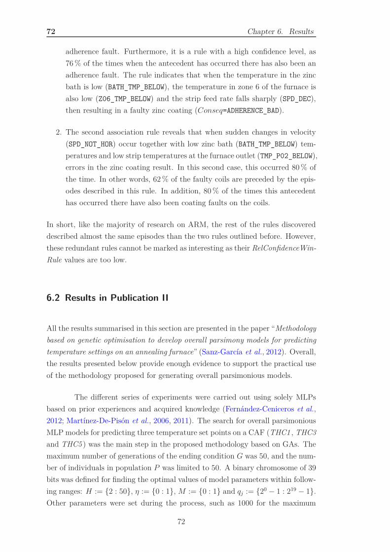
72 Chapter 6. Results
adherence fault. Furthermore, it is a rule with a high confidence level, as
76 % of the times when the antecedent has occurred there has also been an
adherence fault. The rule indicates that when the temperature in the zinc
bath is low (BATH_TMP_BELOW), the temperature in zone 6 of the furnace is
also low (Z06_TMP_BELOW) and the strip feed rate falls sharply (SPD_DEC),
then resulting in a faulty zinc coating (Conseq=ADHERENCE_BAD).
2. The second association rule reveals that when sudden changes in velocity
(SPD_NOT_HOR) occur together with low zinc bath (BATH_TMP_BELOW) tem-
peratures and low strip temperatures at the furnace outlet (TMP_P02_BELOW),
errors in the zinc coating result. In this second case, this occurred 80 % of
the time. In other words, 62 % of the faulty coils are preceded by the epis-
odes described in this rule. In addition, 80 % of the times this antecedent
has occurred there have also been coating faults on the coils.
In short, like the majority of research on ARM, the rest of the rules discovered
described almost the same episodes than the two rules outlined before. However,
these redundant rules cannot be marked as interesting as their RelConfidenceWin-
Rule values are too low.
6.2 Results in Publication II
All the results summarised in this section are presented in the paper “Methodology
based on genetic optimisation to develop overall parsimony models for predicting
temperature settings on an annealing furnace” (Sanz-García et al., 2012). Overall,
the results presented below provide enough evidence to support the practical use
of the methodology proposed for generating overall parsimonious models.
The different series of experiments were carried out using solely MLPs
based on prior experiences and acquired knowledge (Fernández-Ceniceros et al.,
2012; Martínez-De-Pisón et al., 2006, 2011). The search for overall parsimonious
MLP models for predicting three temperature set points on a CAF (THC1 , THC3
and THC5 ) was the main step in the proposed methodology based on GAs. The
maximum number of generations of the ending condition G was 50, and the num-
ber of individuals in population P was limited to 50. A binary chromosome of 39
bits was defined for finding the optimal values of model parameters within follow-
ing ranges: H := {2 : 50}, η := {0 : 1}, M := {0 : 1} and qj := {20 − 1 : 219 − 1}.
Other parameters were set during the process, such as 1000 for the maximum
72
Devel. and Applic. of SC and DM Techniques in Hot Dip Galvanising 73
number of epochs for training models. Additionally, several prior trials were pre-
viously conducted to gain insight into the process adjustments. The following
suitable values were found for the configuration parameters of the GA: elitism
percentage xe = 20 %, mutation factor χ = 39−1 and crossover proportion of
50 %. An ESC was also set up in the same experiments as follows: fraction for
adjusting penalty function xg = 0.2, weighting coefficient of the complexity term
µ = 0.02, period of stability Tg = 10 generations, I = 10 best individuals per
generation and percentage xval = 0.01 % for xCI = 90 %.
In the case study involving the prediction of three temperature set points
on a CAF, the MLP developed with the proposal performed better than those
without it. On the one hand, the testing errors (RMSEtst) for the best models
using optimisation with a complexity function did not exceed 4.5 % (Table 1,
Sanz-García et al., 2012). These models had similar or slightly higher validation
errors (RMSEval) than the others, but significantly lower RMSEtst values pre-
dicting both THC1 and THC5 temperature set points (for THC3, the RMSEtst
was similar to the method without complexity function). On the other hand,
Pearson’s correlation coefficient (R2) was included to evaluate linear dependence
between measures and model predictions. The R2 testing of the MLPs in our pro-
posal clearly records values which better than or equal to those obtained when
the complexity function is omitted.
Interestingly, models trained with complexity control showed a greater
capability for generalisation in two cases (THC1 and THC5 ), i.e. RMSEval was
equal to or even higher than RMSEtst. However, no significant difference was
found between THC3 prediction models with and without complexity function.
The most striking result was the lowest RMSEtst (3.29 %) of the THC5 predic-
tion model using the complexity function that reinforces the usefulness of the
proposal. These interesting results were consistent with the number of neurons
in the hidden layers of the models. The models trained with complexity control
had a total number of neurons equal to or even lower than the models developed
without our proposal (Table 1, Sanz-García et al., 2012). These findings are a
clear consequence of the model´s reduced number of setting parameters.
The representation of the evolution of RMSEval and RMSEtst across
the optimisation process with and without complexity control was crucial to con-
firm the abovementioned results (Figures 9 to 14, Sanz-García et al., 2012). As
observed, both errors were stable and of the same order of magnitude in the
last generation in Figures 10, 11 and 13. By contrast, Figures 9, 12 and 14
73

74 Chapter 6. Results
(Sanz-García et al., 2012) show three processes in which the best solution was
not achieved in the last generation. It is essential to note that the distinction
between the use and non-use of a complexity function is shown in Figures 11 and
14. The most remarkable result to emerge from both figures is that there was no
possibility of finding a subset of steady setting parameters for THC5 prediction
models without including the complexity term in the fitness function (J) of the
GA.
All the plots in Figure 15 (Sanz-García et al., 2012) were also consistent
with previous findings, which represents errors via the aggregation coefficients W
of models. Figure B.3, Figure B.4 and Figure B.5 extend the range of W from 30 to
50, providing more information. First, Figures 15.a and 15.b show RMSEval and
RMSEtst predicting THC1 against the complexity function over generations with
and without complexity control, respectively. Figures 15.c and 15.d represent the
same results for the case of THC3 and, finally, THC5 corresponds to Figures 15.e
and 15.f. Second, the balance between RMSEval and RMSEtst predicting THC1
is higher in Fig. 15.a than in Fig. 15.b because the penalty function reduced the
number of overfitted models. In the case of temperature THC3, Fig. 15.d shows
a lower density than Fig. 15.c in the lower part of the plot, which means a sharp
reduction in computation cost. All these findings are also repeated in Figure B.3,
Figure B.4 and Figure B.5. Our methodology including the complexity function
and an ESC has a clear advantage over standard GAs in Figure B.5 due to the low
density of grey points (RMSEtst ) identified in the lowest values of both axes.
The ESC also reduced the total computation cost for training models
(Table 1, Sanz-García et al., 2012). Our results confirms that the performance of
the resulting models did not decrease, while total computation costs were lower
in two of the three cases studied (Figures 9 to 14, Sanz-García et al., 2012). Nev-
ertheless, the importance of including an ESC appeared surprisingly in Figure 9,
when the best individual in the last generation was not the best model trained.
Figure 9 revealed that the generalisation error of the THC1 model trained in-
cluding the complexity term in J increased from the 30th generation to the last.
In short, Figures 9, 10 and 11 show that we stopped the uncontrolled overfitting.
They offer evidence for considering a key requirement in the combination of the
complexity control and the ESC.
A comparison between the results in the best models obtained (see Table
1, Sanz-García et al., 2012) and the number of the total inputs selected by the
GA-based feature selection (FS) (Table 2, Sanz-García et al., 2012) also shows
74

Devel. and Applic. of SC and DM Techniques in Hot Dip Galvanising 75
that working on a reduced set of attributes has additional benefits. Figure 16
(Sanz-García et al., 2012), Figure B.1 and Figure B.2 show the evolution of the
selected inputs in THC1, THC3 and THC5 prediction models, respectively, for
the 10 best individuals over 50 generations; in other words, they present each
variable’s significance in the accuracy of the 10 best models per generation. In
those figures, the stopping generation is represented using a triangle when the
input was not finally selected and an inverted triangle in the opposite case.
Figure 16 (Sanz-García et al., 2012) shows that the final model trained
with the complexity penalty was developed using only four inputs, and the one
trained without the complexity function had eight inputs; which is the same
as saying that obtained half as much complexity in final models with the pro-
posed complexity control as in those without it. Both methods chose the inputs
VelMed , ThickCoil and TMPP2CNG, but the one with complexity control only
additionally selected P, while the standard method added attributes C, Si and
Mn.
Lastly, a set of attributes stemming from chemical components such as
Cu, B, N and V reflect far less variation in models optimised with the complexity
function than in those without it. Other inputs such as ThickCoil, TMPP2CNG
and VelMed were always significant, so maintaining these attributes as inputs
enhanced the accuracy of the resulting models. A more detailed analysis of these
figures shows that TMPP1 and other chemical components such as Al, Nb and Ti
were never selected. These findings offer compelling evidence for concluding that
our proposal with the complexity term rendered it easier to remove irrelevant
inputs, enhancing the stability of the optimisation process.
6.3 Results in Publication III
All the results described in this chapter are included in the article “Overall models
based on ensemble methods for predicting continuous annealing furnace temper-
ature settings” (Sanz-García et al., 2013).
The steps and criteria of the methodology proposed were applied to mod-
els predicting three temperature set points (THC1, THC3 and THC5 ) for a CAF
on a CHDGL. However, we report only those results concerning 15 different types
of models predicting THC1. The results of THC3 and THC5 prediction models
(30) differ so slightly from those of THC1 that we can suitably summarise the
75

76 Chapter 6. Results
entire information on the evaluation simply by studying THC1 results.
In brief, the prediction models trained were based on three ensemble
schemes as follows: (1) additive regression (Friedman, 1999), (2) bagging (Breiman,
1996), and (3) dagging (Ting, K. M., 1997). Additionally, the five basic compon-
ents of the three EMs selected were the following data-driven models: (1) least
median squared linear regression (LMSQ) (Rousseeuw & Leroy, 1987), (2) linear
regression (LR) (Burnham & Anderson, 1998), (3) Quinlan´s improved M5 al-
gorithm (M5P) (Wang & Witten, 1997), (4) MLP networks (Haykin, 1999), and
(5) SVMs (Smola & Schölkopf, 2004). We wanted to explore different config-
urations within a limited number of trials (Tables 2 and 3, Sanz-García et al.,
2013). We thus generated different models using ranges for the values of the
pre-established setting parameters.
By applying an iterative training process, the results of the evaluation
based on the methodology proposed were obtained, together with the resulting
models. As the main component of the methodology, the evaluation was organised
according to the following criteria: the computation cost of training Ntr models
(t), the root mean squared error (RMSE) and mean absolute error (MAE) in
validation and testing process, and the coefficient of variation (CV ) that measures
model stability by comparing the amount of variance between sets with different
means. Model stability is important for indicating the degree to which a tech-
nique creates repeatable results for different datasets sampled from the same raw
dataset.
Overall, the results are summarised in three tables (Tables 4, 5 and 6,
Sanz-García et al., 2013). Table 4 presents a significant difference between the
training and validation errors of THC1 prediction models based on EMs; Table
5 reports less variation between the training and validation errors of the MLP
models (Martínez-De-Pisón et al., 2010b); and finally, Table 6 presents the most
important difference between the testing errors of the two ensembles and MLP
models.
As expected in tree-based regressors, our evaluation shows that the ap-
plication of any ensemble scheme to M5P generates large models composed of
several specialised trees with hundreds of leaves with significantly lower validation
errors than the rests (RMSEval = 0.0148±0.0009 and MAEval = 0.0071±0.0002,
mean±sd). These results contrast with those obtained from EMs that include
MLP or SVM as their base learner (BL) (except AR-SVM) with higher validation
errors (RMSEval ! 0.0314 ± 0.0014 and MAEval ! 0.0195 ± 0.0002). However,
76
Devel. and Applic. of SC and DM Techniques in Hot Dip Galvanising 77
taking the EMs as a whole, our results show that the application of any en-
semble scheme has a great influence on the standard deviation of the validation
errors, in terms of reducing it in comparison to the corresponding BL reported
by Martínez-De-Pisón et al. (2010b).
Likewise, the training time (t) of the resulting models was evaluated to
check that models were adjusted in a time that was reasonable in proportion to
the size of the modelling dataset (Figure 6, Sanz-García et al., 2013). The time
limit for training Ntr = 10 models was directly related to the size of the training
dataset; and although its value could not be optimal, the limit was established at
t = 50 000 s. The significant differences between different EMs were readily high-
lighted by using comparative percentages of the total training times. As expected,
the experiments proved that the computation costs associated with SVM-based
EMs and MLP-based EMs with high numbers of neurons in the hidden layer were
the highest of all (t > 50 000 s).
The reliability of the models in predicting THC1 from unseen data was
also analysed in the next step (Figure 7, Sanz-García et al., 2013). The best-
performing model in the validation process, which corresponds to the first step,
provided the worst results in the testing process, i.e. M5P-based EMs had a
testing error of RMSEtst = 0.0458 ± 0.0059 and MAEtst = 0.0303 ± 0.0029,
whereas the same model recorded the lowest validation errors of all the models
(RMSEval = 0.0148 ± 0.0009 and MAEval = 0.0071 ± 0.0002) with the same
setting parameters. This phenomenon is graphically represented in the paper,
leaving no doubts that M5P-based EMs have the highest generalisation errors
when working with new coils and, conversely, MLPs with only three neurons in
the hidden layer (MLP03) and MLP-based EMs (AR-MLP, BG-MLP and DG-
MLP models) are the models with the lowest generalisation errors.
Finally, we sought to find those models with the lowest RMSESDtst and
CVtst at the same time. We thus evaluated model stability by comparing RMSESDtst
and CVtst. The results of the evaluation clearly show that the values for MLP-
based EMs are at least four times lower than each single MLP model (Table 6,
Sanz-García et al., 2013) and, therefore, the MLP-based EMs show much greater
stability (Figure 8, Sanz-García et al., 2013).
77

78 Chapter 6. Results
78

Chapter 7
Discussion
This chapter presents the theoretical and practical implications of this work, its
limitations and possible topics for further research. The chapter is organised
following the same sequence as the results (see Chapter 6).
The main goals of this thesis were to seek useful non-trivial rules and
find out which predictive non-parametric methods would be useful and feasible for
producing overall parsimonious regression models from large volumes of industrial
DBs.
As an initial contribution, the main goal was to extract valuable know-
ledge in the form of association rules to reduce the adherence defects affecting
the zinc coating on a CHDGL.
The most striking result that emerged from the data was the extraction
of two rules with very high RelSupportWinRule and RelConfidenceWinRule val-
ues. According to the opinion of the plant experts, both rules were useful for
identifying the causes of adherence failure in a significant percentage of defective
coils. Thus, we believe that this is solid proof that the methodology is capable of
discovering useful hidden knowledge.
Under particular circumstances, this knowledge could also help techni-
cians to evaluate the impact of the process variables on the adherence of the zinc
coating. Moreover, it could even help to identify which parts of the process should
be the focus of corrective and surveillance actions. The parts can be identified
79

80 Chapter 7. Discussion
by analysing all the frequent episodes and the variables that define these.
As expected, the pre-processing phase is highly dependent on eliminating
spurious data, but the experiments also show that some steps in the methodology
depend heavily on the expertise of analysts and engineers. For instance, extreme
caution should be taken when determining the threshold values for the parameters
in Step 2 in which the minima and maxima are obtained. This can be considered
as one of the most critical points in iterative TS processing due to the sensitivity
showed by the parameter R (Fink & Pratt, 2004). In conclusion, the “human
factor” is still vital at several steps in this methodology.
Curiously, the combination of ECLAT, a widely-known algorithm with a
pre-set window and a time lag between the window and the failure to explain (or
consequent of the association rule), generated efficient tools for extracting rules
from the dataset. On the one hand, the use of ECLAT speeded up the search
process and rendered it not necessary to look for more complex algorithms. On
the other hand, the combination of ECLAT and the sliding window enhanced the
efficiency and also the speed of the process because of the drastically reduced size
of the data.
Our experiments were performed using a window width and a time lag,
maintaining both parameters at low values. This allowed us to reduce the size
of the original dataset, with the effect being an increase in the performance of
RelSupportWinRule and RelConfidenceWinRule. We conclude that we made a
good choice in the parameter setup because the causes of the failures tended to
be relatively close in time to the moment of the failure in most of the industrial
processes. It should be noted that low values of RelConfidenceWinRule always
indicate a weak relation between the antecedent and the consequent, as the ante-
cedent appears regardless of whether or not the consequent occurs; by contrast, a
high value of RelConfidenceWinRule indicates a cause-effect relationship between
the antecedent and the consequent. If a good performance is desired, the meth-
odology needs to maintain both RelSupportWinRule and RelConfidenceWinRule
at very high values.
Apart from the previous two rules described in Chapter 6, we found oth-
ers with very high RelSupportWinRule (see Table A.1, Table A.2 and Table A.3).
This tends to happen when the DB contains large volumes of trivial information
and leads to the existence of many redundant episodes with high RelSupportWin-
Rule. Some of these rules were automatically discarded, as they were deemed to
be weaker than the two initial rules because of their lower RelConfidenceWin-
80

Devel. and Applic. of SC and DM Techniques in Hot Dip Galvanising 81
Rule. However, the remaining rules were not finally selected due to the experts´
decision based on their experience in the field. Obviously, the methodology is not
capable of automatically separating useful rules from redundant ones. As this
selection could be highly subjective and depends on the experience of the experts
involved, our findings need to be interpreted with caution, as other potentially
useful rules may still remain in the dataset.
Our methodology reproduced the hidden knowledge properly using the
types of event proposed. We believe that these events were very easy to un-
derstand and use, and they also struck the right balance between information
provided and complexity. Nevertheless, according to the previous paragraph, the
need for manual adjustment was once again crucial. Plant’s technicians and ad-
ditional information from previous papers helped to take the final decision on the
number of variables to be included in the study. In addition, the values of the
search parameters for each one of the events were defined again, with the help of
on-site technicians.
According to Mannila (1997), the purpose of DM is to extract useful
information from large volumes of data, a task that has traditionally been a
manual procedure. Due to the exponential increase in the sizes of databases, there
is a need to propose novelty automated methodologies for this task. Nevertheless,
a fully automated methodology cannot be expected to work properly, since an
expert in the field is required, for instance, to judge the relevance of the findings.
We are aware that the methodology may have other limitations. The
most important one is that it is not possible to estimate how many rules may
still be hidden. A further limitation is that we do not know whether the rules
discovered include all the attributes that explain the adherence defects affecting
the zinc coating. Taken as a whole, the methodology provides useful knowledge
but it is relatively limited because there is no automatic quantification of the
importance or richness of the rules.
On a practical level, the conclusion drawn is that by means of iterative
and interactive adjustments of the pre-processing and segmentation functions
(filters, detection of significant maxima and minima, definition and extraction
of episodes) experts can obtain significant rules more reliably than with fully
automatic rule extraction systems. We therefore consider it worthwhile to make
the effort required to develop tools to facilitate iteration for experts and analysis
software in all pre-processing and time series segmentation tasks.
81

82 Chapter 7. Discussion
It should be noted that the episodes used were only of a “serial” type
because they are easy to manage, although some failures in the process may be
explained solely with parallel episodes. Thus, a future aim is to improve the
methodology by using different type of episode that is more flexible, i.e. non-
serial and non-parallel episode. Another interesting improvement may involve
using the logic of fuzzy associations to seek more flexible sequences akin to human
thought processes. The technique has already been proposed by Luo & Bridges
for frequent episode mining to evaluate the performance of network intrusion
detection systems.
All in all, the methodology applied to the process studied provides know-
ledge that can be used to identify both the main circumstances that affect the
quality of the coating on the coils and the control actions that can be implemen-
ted as a safety measure to resolve the problems arising (Martínez-De-Pisón et al.,
2006; Alfonso-Cendón et al., 2010)
The second contribution focuses on improving the prediction of setting
parameters in continuous processes. The final goal was to develop a methodology
for training overall parsimonious MLP models to predict three temperature set
points (THC1, THC3 and THC5 ) for a CAF on a CHDGL.
Our work centred mainly on validating the usefulness of the semiauto-
matic methodology proposed. Two characteristics distinguish our method from
other optimisations based on GAs. Ours includes a complexity penalty in fitness
function J and also an ESC in the optimisation process.
Note that the problem of developing overall parsimonious MLP net-
works is common place in computer science. It can be found in many rigor-
ous studies published in the field (Schaffer et al., 1990; Chellapilla & Fogel, 1999;
Norgaard et al., 2003; Jones et al., 2005; Siwek et al., 2009; Agarwal et al., 2010).
The goal is to provide a higher capacity to increase the model´s generalisation
capability.
Overall models are those that should not only have a suitable predic-
tion capacity regarding known data, but also be accurate when predicting novel
data. These models were obtained in the last generation of the optimisation
process, as Figures 10, 11 and 13 (Sanz-García et al., 2012) illustrate. Surpris-
ingly, this did not occur in all the experiments. As we can seen in Figures 9, 12
82
Devel. and Applic. of SC and DM Techniques in Hot Dip Galvanising 83
and 14 (Sanz-García et al., 2012), the best solution was not achieved in the last
generation of these optimisation processes. This diversity clearly demonstrates
that standard GA-based optimisation did not automatically generate the expec-
ted overall models. Over-fitting can be observed in the last models generated in
Figures 9, 12 and 14 (Sanz-García et al., 2012).
The first modification made to our methodology was to include the ESC.
This is a supervisory control that can solve the overfitting problems during the
optimisation process, especially when dealing with industrial data. The results
in Table 1 (Sanz-García et al., 2012) allow us to conclude that the generalisation
capacity of the resulting models was enhanced. This statement is consistent with
the literature (Chellapilla & Fogel, 1999; Islam et al., 2001, 2003). Nevertheless,
it must be remarked that in some cases (Figures 12 and 14, Sanz-García et al.,
2012) the control of the evolutionary process using the ESC did not suffice achieve
our initial goals.
One solution to this problem is to include a complexity penalty in the
fitness function J of the GA-based optimisation (Chaturvedi, 2008). Although
the application of this solution has been satisfactory for small DBs, it can also
be applied to complex DBs from industrial processes. We consider this crucial
for determining its usefulness in the support of real industry objectives. As far
as we know, this is currently under analysis.
We wanted to remove this limitation from the optimisation process, we
included the term W in the fitness function J . Figure 11 (Sanz-García et al.,
2012) shows the effect of this term in comparison to Figure 14 (Sanz-García et al.,
2012), in which the complexity penalty is not used. We conclude that W guaran-
tees the existence of at least one stable period to achieve more accurate results.
The benefits of the inclusion of W in the fitness function J are due to the reduc-
tion in the number of neurons in the hidden layer of the MLP models. Models
were less complex and, consequently, their training time is also reduced.
These results prove that our method can significantly decrease the risk
of overfitting by training the MLPs in the cases in which it was applied. Con-
sequently, we show that overall parsimonious models can be generated by using
both the complexity term and the ESC. These findings are useful for reinforcing
the application of this proposal in the steel industry.
A well-known disadvantage of using GAs is the need for massive data
processing that always involves high computation costs (Goldberg, 1989). Just
83
84 Chapter 7. Discussion
as the complexity penalty was crucial for reducing the training time of models,
the ESC has also turned out to be very useful for reducing the computation cost
of the optimisation in two (THC1 and THC3 ) of the three processes. In case of
THC5, the best models were always found in the last generation. The reason for
these rather contradictory results is still not entirely clear. We assume that the
complexity of the DB may have some influence.
With no loss of model accuracy, total computation cost for training the
models was always the same or lower using these parameters than without them.
We conclude that the combination of both the two modifications (W and ESC)
is an appropriate solution.
In a previous paper, Martínez-De-Pisón et al. (2010b) report substantial
improvements in the reduction of the number of input variables related to chem-
ical composition of steel by using principal component analysis (PCA) (Pearson,
1901; Hotelling, 1993). PCA has shown itself capable of transforming fourteen
initial variables for the chemical composition of steel into a small set of seven
uncorrelated inputs. The disadvantage of applying this technique is quiet clear.
The interpretation of the resulting models is more difficult as raw variables are
no longer being used.
GAs have been widely used for FS in a wrapper approach in many pre-
vious articles (Guerra-Salcedo & Whitley, 1999; Opitz, 1999; Tang & Honavar,
1997). In our method, GA-based FS has been used to create a subset of input
variables from an initial set of all the variables without any exception. The results
obtained (Table 1, Sanz-García et al., 2012) show an increase in model accuracy
using GA-based FS. The lower errors were due to a less collinearity between the
data. This has also leads to higher parsimony in the models.
Consequently, the new method seems more suitable for selecting solely
those variables needed to generate parsimonious models. The aim was to reduce
the number of variables for the chemical composition of steel. We thus conclude
that the use of GA-based FS has more advantages than PCA. In addition, it
should be noted that GA-based FS is more robust than PCA because the former
does not assume that the scores from its models must be normally distributed.
Our results also confirm that GA-based FS enhanced the interpretation
of the final models. The interpretation of the selected variables can provide plant
experts with more information about the annealing treatment and the influence
certain particular variables have on it. Using our methodology makes it easier to
84

Devel. and Applic. of SC and DM Techniques in Hot Dip Galvanising 85
find the most significant variables for generating more parsimonious models.
The inputs VelMed, TMPP1, WidthCoil, ThickCoil and TMPP2CNG
were included in the models from a previous paper (Martínez-De-Pisón et al.,
2010b) with no prior significance rating. In our methodology, VelMed, ThickCoil
and TMPP2CNG are also maintained as inputs, so these attributes clearly en-
hance model accuracy. These statements are consistent with previous research,
where these are the only inputs to have been selected (Martínez-De-Pisón et al.,
2010b). However, in this thesis, TMPP1 was always discarded in all cases. One
conclusion is that TMPP1 is redundant and not therefore relevant for use as an
input.
The input TMPP1 was discarded together with Al, Nb and Ti, which
finally became irrelevant attributes forthcoming from chemical composition. The
inputs C, Si and Mn have the same performance together as the first model
with only the variable P. This shows that both fitness functions can produce
high performance models, but only our proposal generates a parsimonious model.
In these cases, according to Guyon & Elisseeff (2003), some variables that are
useless by themselves can be useful together. A similar behaviour has been ob-
served for THC3 and THC5 prediction models (see Supplementary Material in
Sanz-García et al., 2012).
We are aware that our methodology has two main limitations: the first is
that it is not as fully automatic as we would have linked. The starting operations
for setting the parameters of the optimisation process are not automatically per-
formed. Iterative work is always required to achieve good results. This apparent
lack of automation at the starting point means that the method is finally clas-
sified as semiautomatic. However, it does not need any more adjustments once
its setting parameters have been adjusted. Moreover, the method can update
models by itself when novel data are collected from new operating conditions.
This property means that it can keep operating for a significant length of time
without human assistance.
The second limitation is the difficulty in estimating the values of the
setting parameters at the starting point of our method. It is extremely difficult
to estimate the threshold needed for the complexity function. Again, human
assistance is absolutely necessary for the starting settings.
The two limitations described here are clear evidence of the difficulty in
creating autonomous systems. It is still a challenging task to develop systems that
85

86 Chapter 7. Discussion
auto-update their setting parameters to deal with novel data. On real produc-
tion lines, the integration of the tools based on this approach remains somewhat
difficult.
It is important to mention that the chromosome of the GA selected uses
a binary format to represent the model parameters to be optimised. Binary-
coded GAs suffer from the problem of Hamming Cliffs (Gen & Cheng, 2000). An
excessive number of bits sometimes need to be changed to make small changes
in a parameter. This clearly reduces the efficiency of the GA. Although the
performance was not perfect, we still believe that the binary-coded chromosome
to be a satisfactory solution.
As Grefenstette (1986) proposed, the problem can be avoided by using
gray code instead of binary. However, we decided to keep the population size at
high values in our case. We consider that this suffices to reduce the disadvant-
ages of optimising real-valued parameters using a binary-coded GA. We agree
that a real-coded chromosome is more suitable for continuous search space than
its binary-coded counterpart. Nevertheless, including the FS process in the op-
timisation process tips the balance towards the use of the binary. In contrast to
earlier researches (Goldberg et al., 1992), we understand the binary-coded chro-
mosome has certain advantages when combining optimisation with GA-based
FS.
Difficulties still remain in the way of dealing with noisy data. Outliers
and empty values can be easily filtered, but noise is particularly challenging prob-
lem. Future work will explore the influence of the noise on training data. Noise
is very difficult to remove and industrial plants are characterised by a high ratio
of noise in the variables measured. It is well-known that noise drastically reduces
model accuracy. It also makes it difficult to glean meaningful knowledge from the
data (Yang & Wu, 2006).
The methodology was implemented using only MLP networks. There are
many types of ANNs such as Bayesian networks and RBFNs, among others. As
far as we know, they might be better suited to other industrial processes. For
that reason, we are currently in the process of extending the proposal to create
a generic tool that includes other models. The main requierement is that model
complexity hast to be controlled as in SVM-based models or MLP-based EMs.
In short, we believe that the results obtained provide evidence to con-
firm the efficiency and reliability of this advanced methodology compared with a
86

Devel. and Applic. of SC and DM Techniques in Hot Dip Galvanising 87
standard optimisation based on GAs.
Finally, the findings in third contribution provide enough support for
using EMs to predict set points for online control systems.
Industrial processes such as CHDGLs tend to generate very large, noisy
DBs that always entail a loss of accuracy, wasted time and storage problems.
When dealing with these problems, the scalability of models is needed to discover
knowledge due to the size of these DBs (Schlang & Lang, 2001; Paliwal & Kumar,
2009). EMs have been successfully applied in many small-scale cases. As far as
we know, selecting the suitable scheme for scaling up to large industrial DBs still
poses a challenge (Rokach, 2010).
The comparative methodology proposed for evaluating model perform-
ance clearly has an advantage over the previous ones. It gives robust evidence
on the real performance of models, which has proved crucial for identifying those
models with the highest generalisation capacity but also with low computation
cost. The main explanation for this improvement is the inclusion of new metrics
and the repetition of the testing process (by bootstrapping with the testing data
a total of N = 10 times).
In addition, our comparative study took a different point of view because
it focused solely on three ensemble schemes and five BLs. However, we modified
model parameters while those in other studies often remain unchanged. Addi-
tionally, we did not use a small dataset that was from repositories or well-known
databases; instead, all our data came from the CHDGL. This source generates
data with great heterogeneity, imbalance and skewness that make it more difficult
to achieve an accurate prediction.
First, the results from the evaluation of single data-driven models, which
are also called base learners (BLs) in ensemble learning literature, were required in
order to discuss advantages and disadvantages by comparing them with the EMs
proposed. These results were obtained from previous experiments carried out
by Martínez-De-Pisón et al. (2010b). Our results using a comparative evaluation
prove that EMs are better overall models because of their lower generalisation
error. This is consistent with several previous papers, such as Barai & Reich
(1999), Mevik & Segtnan (2004) or Siwek et al. (2009).
87
88 Chapter 7. Discussion
It is important to stress that our results are in a close agreement with
several performance assessments of EMs reported in the literature (Breiman, 1996;
Opitz & Maclin, 1999; Minowa, 2008). Although the good performance of EMs
has been well reported in computer science (Hand et al., 2001; Witten & Frank,
2005; Nisbet et al., 2009), we believe our results show that the benefits of using
EMs to deal with small datasets could be extended to complex industrial DBs..
M5P and MLP networks are two examples of unstable learning algorithms,
in which small perturbations in the training dataset can cause significant changes
in predictions. In 1996, Breiman showed the effectiveness of applying bagging
for combining these BLs. Remarkably, M5P-based EMs performed badly in our
experiments. Although this finding differs to some extent from those of Breiman
(1996), it could nevertheless be argued that a good explanation of why MLP-
based EMs performed better is found in Barai & Reich (1999) and corroborated
by Yang et al. (2011).
Note that MLP-EMS have attracted the attention of many researchers
in modelling. They appear to be a very promising approach for reducing the gen-
eralisation error of models. In general, these EMs are constructed by developing
a number of standard ANNs for regression problems (Witten & Frank, 2005).
Several studies have already provided valuable information about the poten-
tial of many ensemble schemes. Bauer & Kohavi (1999); Opitz & Maclin (1999);
Galar et al. (2011) are examples working on classification tasks and Pardo et al.
(2010) on regression.
What is surprising is the fact that MLP networks such as BLs were the
best in all the ensemble schemes evaluated. This might be because of the well-
known ability of MLP networks have to accurately predict continuous output
variables. However, our results also suggest that this property is maintained
using the MLP networks as BL. This matches well with previous results reported
by Niu et al. (2011) and Yang et al. (2011) and also confirms the initial findings
in Pardo et al. (2010). Another explanation may be the ability of MLP networks
to perform an overall global approximation, while other models such as RBFNs
are typically local approximation methods.
The MLP networks with only three neurons in the hidden layer (MLP03)
and MLP-based EM (AR-MLP, BG-MLP and DG-MLP) recorded the highest
generalisation capacity. The main reason is that they struck a good balance
between validation and testing errors. This is because of their less complex struc-
ture, which means they are not so specialised as in previously known data. It
88
Devel. and Applic. of SC and DM Techniques in Hot Dip Galvanising 89
should be noted that some of these less comlex models sometimes even present
fewer testing errors than validation ones. We assume that this happens because
the validation dataset is more complex than the testing one in these cases.
Our results also show that MLP-based EMs are able to make similar
predictions even in changing conditions, such as slight changes in inputs and
variations in the setting parameters of models. This suggests that MLP-based
EMs are more reliable than the other EMs studied.
In contrast, M5P-based EMs recorded a clear trend for overfitting. We
were not successful in avoiding this problem, even when modifying the config-
uration parameters of the BL or the pruning conditions for the model trees. In
modelling literature (Seni & Elder, 2010), M5P is considered an unstable model,
and, consequently, it records very low validation errors. However, M5P as BL
is clearly unsuitable for working in changing environments that generate large
volumes of novel data. This phenomenon is graphically represented in the paper
(Figures 5 and 7, Sanz-García et al., 2013), leaving no doubt that M5P-based
EMs have the lowest generalisation capacity of all the models.
The AR-SVM model and the EMs including LSMQ or LR as BLs failed
to ensure enough accuracy in the prediction of temperature set points. The SVM,
LR and LSMQ models are classified as stable, and they are included in the same
group as k-nearest neighbour (k-NN) regressors (Breiman, 1996). As reported by
Breiman (1994), the results that we have obtained indicate that any ensemble
scheme using a stable algorithm is extremely accurate.
All the EMs developed seem to have recorded significant improvements in
all features, but the reality is that their computation costs are always higher. The
cost is sometimes even considered excessive for a prediction model that should be
implemented in a real-time control system. For instance, the experiments prove
that the computation costs associated with SVM-based EMs and MLP-based
EMs with high numbers of neurons in the hidden layer are unreasonable. This
result has further strengthened our conviction that using MLP with few neurons
in the hidden layer and a low number of iterations in the learning process would
be crucial for obtaining overall models (Martínez-De-Pisón et al., 2010b, 2011).
Consequently, the improvement in both accuracy and generalisation ca-
pacity of EMs entails mainly extra computation time, lower intelligibility and
higher complexity than single models. However, those BLs that make up EMs
can be independently trained in parallel, decreasing the training time of EMs.
89

90 Chapter 7. Discussion
Further research could be conducted in at least two areas that build on
the lastest methodology presented. First of all, the use of a weighted average
method instead of simple average would be combine the outputs with different
weights for each model developed. These weights could be calculated by some
kind of regression modelling, such us partial least squares regression. In addition,
another kind of dynamic ANN could be used to generate models that are less
correlated and have higher variation or disparity between them. This could be
effective for improving the generalisation capability and also the effectiveness of
models dealing with novel data.
In short, we consider that the methodology proposed provides valuable
information that directly enables to be taken regarding the most interesting model
for developing a specific problem; and in our particular case study the information
obtained and the direction of the results reveal trends in modelling process that
could be of great help to plant engineers.
In conclusion, all these findings allowed us to suggest that the entire
process of applying the methodologies proposed in this thesis could be used to
extract valuable knowledge from the CHDGL database studied. While not all the
results were significant in this thesis, their general direction points to the major
possibilities the implementation of DM methodologies could have for assisting in
the complex task of improving industrial processes.
90
Chapter 8
Conclusions
The methodologies proposed may be applied to CHDGLs to discover useful know-
ledge that helps plant engineers to improve galvanising processes. Our results re-
veal the huge number of unexplored possibilities that this knowledge can provide
for developing models and decision support systems, among others.
This thesis was carried out with a view to improving the existing method-
ologies in two main aspects: finding association rules for explaining failures in the
galvanising lines and developing better models for predicting CAF temperature
set points in the CAF on the line.
The research presented in this thesis provides the following findings:
• A methodology based on simple pre-processing, segmentation and a search
for hidden knowledge on the basis of TS that can be easily applied to the
enhancement of production processes. The pre-processing and segmentation
of TS linked to the use of ARM is shown to be extremely useful when
searching for hidden knowledge in the data logs of industrial processes,
which may help to reduce failures in production lines.
• A methodology based on data-driven methods for designing overall parsimo-
nious models to predict CAF temperature set points. The proposed meth-
odology makes it easier for plant engineers to deal with continuous product
changes, spending less time on adjusting models and reducing downtime
costs. The main advantages of this methodology are the reduced complex-
ity of the final models, better generalisation capacity and the computation
91

92 Chapter 8. Conclusions
time saved, whereby it can be incorporated it into a CAF’s online control
system.
• A comparative methodology for selecting better overall data-driven models
to predict temperature set points for a CAF on a CHDGL. The compar-
ative evaluation proves that the use of MLP network as BL is the best
choice for generating the best-performing models, i.e. AR-MLP, BG-MLP
and DG-MLP. In addition, it provides support for the final recommenda-
tions on using EMs as a regression technique. Their main advantages are
high efficiency and reliability in terms of computation cost, generalisation
capacity and ease for determining the best model configuration.
All in all, the methodologies described can make it easier for plant engineers to
deal with continuous product changes, spending less time on adjusting the line,
and reducing the time and cost of solving problems on production lines when
dealing with new products.
92
Bibliography
(1998). Hot Dip Coating Line for ACERALIA, Spain. 030608222 Rev 1.0. Drever
International S.A., tech report of the mathematical model.
(2006). Hot-dip Galvanizing for Corrosion Protection: A Specifiers Guide. Amer-
ican Galvanizers Association, Centennial, CO, USA.
(2006). Iron and Steel Industry in 2004. Technical report, Organisation for eco-
nomic co-operation and development (OECD), Paris, France.
(2010). Romania Steel and Iron Report. Technical report, Intellinews, Bucarest,
RO.
Abdel-Aal, R.E. (2008). Univariate modeling and forecasting of monthly energy
demand time series using abductive and neural networks. Computer & Indus-
trial Engineering, 54(4), pp. 903–917.
Agarwal, A., Tewary, U., Pettersson, F., Das, S., Saxén, H. & Chakraborti, N.
(2010). Analysing blast furnace data using evolutionary neural network and
multiobjective genetic algorithms. Ironmaking and Steelmaking, 37(5), pp. 353–
359.
Agarwal, K. & Shivpuri, R. (2012). An on-line hierarchical decomposition based
bayesian model for quality prediction during hot strip rolling. ISIJ Interna-
tional, 52(10), pp. 1862–1871.
Agrawal, R. & Srikant, R. (1994). Fast algorithms for mining association rules.
In: Proceedings of the 20th international conference on very large databases,
Santiago, Chile., pp. 487–499.
Aldrich, C. (2002). Exploratory analysis of metallurgical process data with neural
93
94 Bibliography
networks and related methods, volume 12 of Process Metallurgy. Amsterdam,
EU: Elsevier Science Ltd., 1st edition.
Alfonso, F., Martínez, L., Pérez, A. & Valente, J. (2012). Cooperation between
expert knowledge and data mining discovered knowledge: Lessons learned.
Expert Systems with Applications, 39(8), pp. 7524–7535.
Alfonso-Cendón, J., Castejón-Limas, M., Sanz-García, A., Fernández-Ceniceros,
J. & Fernández-Martínez, R. (2010). Re-implementation of amore package. In:
Proceedings of the XIV International Congress on Project Engineering. Madrid,
Spain, 2010.
Argyropoulos, S.A. (1990). Artificial intelligence in materials processing opera-
tions: A review and future directions. ISIJ Int (Iron Steel Inst Jpn), 30(2), pp.
83–89.
Atallah, M.J., Gwadera, R. & Szpankowski, W. (2004). Detection of significant
sets of episodes in event sequences. In: Proceedings of the 4th IEEE Int. Conf.
on Data Mining (ICDM 2004), Brighton, UK, pp. 3–10.
Barai, S. & Reich, Y. (1999). Ensemble modelling or selecting the best model:
many could be better than one. Artif Intell Eng Des Anal Manuf, 13, pp. 377–
386.
Bauer, E. & Kohavi, R. (1999). An empirical comparison of voting classification
algorithms: Bagging, boosting, and variants. Machine Learning, 36, pp. 105–
139.
Bian, J., Zhu, Y., Liu, X.H. & Wang, G.D. (2006). Development of hot dip
galvanized steel strip and its application in automobile industry. Journal of
Iron and Steel Research International, 13(3), pp. 47–50.
Bloch, G. & Denoeux, T. (2003). Neural networks for process control and optim-
ization: Two industrial applications. ISA Transactions, 42, pp. 39–51.
Bloch, G., Sirou, F., Eustache, V. & Fatrez, P. (1997). Neural intelligent control
for a steel plant. IEEE Transactions on Neural Networks, 8(4), pp. 910–918.
Breiman, L. (1994). Heuristics of instability in model selection. Technical report,
Statistics Department, University of California, Berkeley, USA.
94

Devel. and Applic. of SC and DM Techniques in Hot Dip Galvanising 95
Breiman, L. (1996). Bagging predictors. Machine Learning, 24(2), pp. 123–140.
Burnham, K.P. & Anderson, D.R. (1998). Model selection and inference: a prac-
tical information-theoretic approach. Springer.
Casas-Garriga, G. (2003). Discovering unbounded episodes in sequential data.
In: Proceedings of the 7th Eur. Conf. on Principles and Practice of Knowledge
Discovery in Databases (PKDD’03), Cavtat-Dubvrovnik, Croatia, pp. 83–94.
Chapman, P., Clinton, J., Kerber, R., Khabaza, T., Reinartz, T., Shearer, C. &
Wirth, R. (2000). Crisp-dm 1.0: Step-by-step data mining guide.
Chaturvedi, D. (2008). Soft Computing: Techniques and its Applications in Elec-
trical Engineering, volume 103 of Studies in Computational Intelligence. Berlin,
Germany: Springer Berlin / Heidelberg.
Chellapilla, K. & Fogel, D. (1999). Evolution, neural networks, games, and intel-
ligence. In: IEEE, volume 87, pp. 1471–1496.
Chen, L., Fourmentin, R. & McDermid, J. (2008). Morphology and kinematics of
interfacial layer formation during continuous hot-dip galvanising and galvan-
nealing. Metallurgical and Materials Transactions A, 3A, pp. 2128–2142.
Chen, Y.C., Jiang, J.C., Peng, W.C. & Lee, S.Y. (2010). An efficient algorithm
for mining time interval-based patterns in large databases. In: Proceedings of
the 19th ACM international conference on Information and knowledge man-
agement, Toronto, Ontario, Canada, pp. 49–58.
Cheng, A., Rorick, F. & Poveromo, J.J. (2009). Recent developments in north
american ironmaking. In: 5th International Congress on the Science and Tech-
nology of Ironmaking (ICSTI), Shanghai.
Choo, A., Linderman, K. & Schroeder, R. (2007). Method and context perspect-
ives on learning and knowledge creation in quality management. Journal of
Operations Management, 25(4), pp. 918–931.
Choudhary, A., Harding, J. & Tiwari, M.K. (2009). Data mining in manufactur-
ing: a review based on the kind of knowledge. Journal of Intelligence Manu-
facturing, 20(501), p. 521.
Core, B. & Goethals, B. (2010). Mining association rules in long sequences. In:
95

96 Bibliography
Lecture Notes in Computer Science, LNAI, volume 6118 (PART1), Springer
Berlin / Heidelberg, pp. 300–309.
Cox, I., Lewis, R., Ransing, R., Laszczewski, H. & Berni, G. (2002). Application of
neural computing in basic oxygen steelmaking. Journal of Materials Processing
Technology, 120, pp. 310–315.
Das, G., Gunopulos, D. & Mannila, H. (1997). Finding similar time series. In:
Proceedings of the First European Symposium on Principles and Practice of
Knowledge Discovery in Databases, pp. 88–100.
Das, G., Lin, K.I., Mannila, H., Renganathan, G. & Smyth, P. (1998). Rule
discovery from time series. In: Proceedings of the Fourth ACM SIGKDD Inter-
national Conference on Knowledge Discovery and Data Mining, AAAI Press,
pp. 16–22.
de Medeiros, F.T.P., Noblat, S.J.X. & Fileti, A.M.F. (2007). Reviving traditional
blast furnace models with new mathematical approach. Ironmaking and Steel-
making, 34(5), pp. 410–414.
del Jesús, M., Gámez, J. & Puerta, J. (2009). Evolutionary and metaheuristics
based data mining. Soft Computing, 13, pp. 209–212.
Dote, Y. & Ovaska, S.J. (2001). Industrial applications of soft computing: A
review. In: Proceedings of the IEEE, volume 89, IEEE Society, pp. 1243–1265.
Dürr, W., Irle, M. & Dornseifer, T. (2005). Operating experience with an online
measurement system for mechanical properties within a hot-dip galvanizing
line. In: Materials Science and Technology 2005 Conference, volume 4, Pitts-
burgh, PA, pp. 87–94.
Erickson, G.S. & Rothberg, H.N. (2009). Intellectual capital in business-to-
business markets. Industrial Marketing Management, 38, pp. 159–165.
Femminella, O., Starink, M., Brown, M., Sinclair, I., Harris, C. & Reed, P. (1999).
Data pre-processinglmodel initialisationin neurofuzzy modelling of structure-
property relationships in al-zn-hng-cu alloys. ISIJ Int (Iron Steel Inst Jpn),
39(10), pp. 1027–1037.
Fernández-Ceniceros, J., Sanz-García, A., Antoñanzas-Torres, F. & Martínez-de
Pisón-Ascacibar, F. (2012). Multilayer-perceptron network ensemble modeling
96
Devel. and Applic. of SC and DM Techniques in Hot Dip Galvanising 97
with genetic algorithms for the capacity of bolted lap joint. In: Hybrid Artificial
Intelligent Systems, volume 7208 of Lecture Notes in Computer Science (eds.
E. Corchado, V. Snásel, A. Abraham, M. Wozniak, M. Graña & S.B. Cho),
Springer Berlin / Heidelberg, pp. 545–556.
Ferreiro, S., Sierra, B., Irigoien, I. & Gorritxategi, E. (2011). Data mining for
quality control: Burr detection in the drilling process. Computer & Industrial
Engineering, 60(4), pp. 801–810.
Fink, E. & Pratt, K. (2004). Indexing of compressed time series. Data Mining In
Time Series Databases. World Scientific, New York, pp. 51–78.
Friedman, J.H. (1999). Stochastic Gradient Boosting. Technical report, Stanford
University.
Galar, M., Fernández, A., Barrenechea, E., Bustince, H. & Herrera, F. (2011).
An overview of ensemble methods for binary classifiers in multi-class problems:
Experimental study on one-vs-one and one-vs-all schemes. Pattern Recognition,
44, pp. 1761–1776.
Gen, M. & Cheng, R. (2000). Genetic algorithms and engineering optimization.
Wiley Series in Engineering Design and Automation, Canada: John Wiley &
Sons, Inc., 1st edition.
Giudici, P. & Figini, S. (2009). Applied Data Mining for Business and Industry.
John Wiley & Sons, Ltd, 2nd edition.
GmbH, Q. (2009). Software makes metals decision-making easy. Steel Times In-
ternational, p. 32.
Goldberg, D. (1989). Genetic Algorithms in Search, Optimization and Machine
Learning. MA: Addison-Wesley, Reading.
Goldberg, D., Deb, K. & Clark, J. (1992). Genetic algorithms, noise, and the
sizing of populations. Complex Systems, 6, pp. 333–362.
Gonzalez, M., Trevino, A., Bailleul, M. & Nlome-Nze, F. (2006). Automatic sur-
face inspection for galvanized products at imsa mex. In: AISTech 2006 Con-
ference Proceedings, volume 2, pp. 199–201.
González-Marcos, A. (2007). Desarrollo de técnicas de minería de datos en pro-
97
98 Bibliography
cesos industriales: Modelización en líneas de producción de acero. Ph.D. thesis,
Universidad de La Rioja.
Grefenstette, J. (1986). Optimization of control parameters for genetic al-
gorithms. IEEE Transactions on Systems, Man, and Cybernetics, 16, pp. 122–
128.
Guerra-Salcedo, C. & Whitley, L. (1999). Genetic approach to feature selection for
ensemble creation. In: International Conference on Genetic and Evolutionary
Computation, pp. 236–243.
Guyon, I. & Elisseeff, A. (2003). An introduction to variable and feature selection.
J. Mach. Learn. Res., 3, pp. 1157–1182.
Haji, A. & Assadi, M. (2009). Fuzzy expert systems and challenge of new product
pricing. Computers & Industrial Engineering, 56(2), pp. 616–630.
Han, J. & Kamber, M. (2006). Data Mining: Concepts and Techniques. San
Francisco, CA, USA: Morgan Kaufmann Publishers Inc., 2nd edition.
Hand, D., Mannila, H. & Smyth, P. (2001). Principles of Data Mining. Cam-
bridge, Massachusetts: The MIT Press.
Harding, J., Shahbaz, M., Srinivas, A. & Kusiak, A. (2006). Data mining in
manufacturing: a review. Journal of Manufacturing Science and Engineering,
128, pp. 969–976.
Harms, S.K., Deogun, J. & Tadesse, T. (2002). Discovering sequential association
rules with constraints and time lags in multiple sequences. In: Proceedings of
the 2002 International Symposium on Methodologies for Intelligent Systems,
Berlin, Heidelberg, pp. 432–441.
Harvey, M.G. & Lusch, R.F. (1999). Balancing the intellectual capital books:
Intangible liabilities. European Management Journal, 17(1), pp. 88–92.
Hassan, M., El-Sharief, M., Aboul-Kasem, A., Ramesh, S. & Purbolaksono, J.
(2012). A fuzzy model for evaluation and prediction of slurry erosion of 5127
steels. Materials & Design, 39(0), pp. 186–191.
Haykin, S. (1999). Neural Networks: A Comprehensive Foundation. Prentice Hall.
98

Devel. and Applic. of SC and DM Techniques in Hot Dip Galvanising 99
He, S.G., He, Z., Wang, G.A. & Li, L. (2009). Data Mining and Knowledge
Discovery in Real Life Applications, chapter Quality Improvement using Data
Mining in Manufacturing Processes. Vienna, Austria: I-Tech, pp. 357–372.
Hodgson, P. (1996). Microstructure modelling for property prediction and control.
Journal of Materials Processing Technology, 60, pp. 27–33.
Hoppe, H.C. (2002). The timing of new technology adoption: Theoretical models
and empirical evidence. The Manchester School, 70(1), pp. 56–76.
Hotelling, H. (1993). Analysis of a complex of statistical variables into principal
components. J. Educ. Psychol., 24, pp. 417–441.
Huang, K.Y. & Chang, C.H. (2007). Efficient mining of frequent episodes from
complex sequences. Information Systems, 33(1), pp. 96–114.
Islam, M.M., Shahjahan, M. & Murase, K. (2001). Exploring constructive al-
gorithms with stopping criteria to produce accurate and diverse individual
neural networks in an ensemble. In: IEEE International Conference on Sys-
tems, Man, and Cybernetics, volume 3, pp. 1526–1531.
Islam, M.M., Yao, X. & Murase, K. (2003). A constructive algorithm for training
cooperative neural network ensembles. IEEE Transactions on Neural Networks,
14(4), pp. 820–834.
Jaluria, Y. (1988). Numerical simulation of the transport processes in a heat
treatment furnace. Int. J. Numer. Methods Eng., 25, pp. 387–399.
Jelali, M. (2006). An overview of control performance assessment technology and
industrial applications. Control Engineering Practice, 14, pp. 441–446.
Jones, D.M., Watton, J. & Brown, K.J. (2005). Comparison of hot rolled steel
mechanical property prediction models using linear multiple regression, non-
linear multiple regression and non-linear artificial neural networks. Ironmaking
and Steelmaking, 32(5), pp. 435–442.
Kam, P.S. & Fu, A.C. (2000). Discovering temporal patterns for interval-based
events. In: Proceedings of the 2nd International Conference on Data Warehous-
ing and Knowledge Discovery (DaWaK’00), London, UK, pp. 317–326.
99
100 Bibliography
Kantardzic, M. (2011). Data Mining: Concepts, Models, Methods, and Al-
gorithms. Hoboken, NY, USA: John Wiley & Sons, Inc., 2nd edition.
Köksal, G., Batmaz, E. & Testik, M.C. (2011). A review of data mining applica-
tions for quality improvement in manufacturing industry. Expert Systems with
Applications, 38(10), pp. 13448–13467.
Kuru, E. & Kuru, L. (2011). Fuzzy inference system controls in hot dip galvanizing
lines. In: Proceedings of the 7th International Conference on Electrical and
Electronics Engineering (ELECO), volume 2, Bursa, Turkey, pp. 400–404.
Kusiak, J. & Zuziak, R. (2002). Modelling of microstructure and mechanical
properties of steel using the artificial neural network. Journal of Materials
Processing Technology, 127, pp. 115–121.
Laxman, S., Sastry, P.S. & Unnikrishnan, K.P. (2004). Fast algorithms for fre-
quent episode discovery in event sequences. In: 3rd Workshop on Mining Tem-
poral and Sequential Data, Seattle, WA.
Lee, D., Moon, C., Moon, S. & Park, H. (2009). Development of healing con-
trol technology for reducing breakout in thin slab casters. Control Engineering
Practice, 17, pp. 3–13.
Lee, P.D., Ramirez-Lopez, P.E., Mills, K.C. & Santillana, B. (2012). Review: The
“butterfly effect” in continuous casting. Ironmaking and Steelmaking, 39(4), pp.
244–253.
Lengnick-Hall, C.A. & Griffith, R.J. (2011). Evidence-based versus tinkerable
knowledge as strategic assets: A new perspective on the interplay between in-
novation and application. Journal of Engineering and Technology Management,
28, pp. 147–167.
Li, G.Y. & Dong, M. (2011). A wavelet and neural networks based on fault dia-
gnosis for hagc system of strip rolling mill. Journal of Iron and Steel Research,
International., 18(1), pp. 31–35.
Li, J., Yan, Y., Guo, X., Wang, Y. & Wei, Y. (2011a). On-line control of strip sur-
face quality for a continuous hot-dip galvanizing line based on inherent property
of thin plate. Journal of Mechanical Engineering, 47(9), pp. 60–65.
Li, J., Feng, H. & Li, S. (2011b). Wavelet prediction fuzzy neural network of the
100
Devel. and Applic. of SC and DM Techniques in Hot Dip Galvanising 101
annealing furnace temperature control. In: Proceedings of the 2011 Interna-
tional Conference on Electric Information and Control Engineering (ICEICE),
Wuhan, China, pp. 940–943.
Li, S., Chen, Q. & Huang, G.Y. (2006). Dynamic temperature modeling of con-
tinuous annealing furnace using ggap-rbf neural network. Neurocomputing, 69,
pp. 523–536.
Liao, S.H., Chu, P.H. & Hsiao, P.Y. (2012). Data mining techniques and applic-
ations - a decade review from 2000 to 2011. Expert Systems with Applications,
39(12), pp. 11303–11311.
Liu, L., Wang, A., Sha, M., Sun, X. & Li, Y. (2011). Optional svm for fault
diagnosis of blast furnace with imbalanced data. ISIJ Int (Iron Steel Inst Jpn),
51(9), pp. 1474–1479.
Lu, Y.Z. & Markward, S. (1997). Development and application of an integrated
neural system for an hdcl. IEEE Transactions on Neural Networks, 8(6), pp.
1328–1337.
Lücking, F. (2011). First installation of the new web-based quality analysis and
reporting software. Metallurgical Plant and Technology, 5, pp. 82–85.
Luo, J. & Bridges, S.M. (2000). Mining fuzzy association rules and fuzzy frequent
episodes for intrusion detection. International Journal of Intelligent Systems,
15(8), pp. 687–703.
Madureira, N.L. (2012). The iron industry energy transition. Enrgy Policy, 50,
pp. 24–34.
Maimon, O. & Rokach, L. (2008). Soft Computing for Knowledge Discovery and
Data Mining, chapter Introduction to soft computing for knowledge discovery
and data mining. Springer, pp. 1–16.
Malerba, F. (2007). Innovation and the dynamics and evolution of industries:
Progress and challenges. International Journal of Industrial Organization, 25,
pp. 675–699.
Mannila, H. (1997). Methods and problems in data mining. In: 6th International
Conference on Database Theory (ICDT 1997), volume 1186 of Lecture Notes
101
102 Bibliography
in Computer Science (eds. F.N. Afrati & P.G. Kolaitis), Springer- Verlag, pp.
41–55.
Mannila, H., Toivonen, H. & Verkamo, A. (1997). Discovery of frequent episodes
in event sequences. Data Mining Knowledge Discovery, 1(3), pp. 259–289.
Marakas, G.M. (1998). Decision Support Systems in the 21st Century. Prentice
Hall.
Martínez-De-Pisón, F.J. (2003). Optimización mediante técnicas de minería de
datos del ciclo de recocido de una línea de galvanizado. Ph.D. thesis.
Martínez-De-Pisón, F.J., Alba-Elías, F., Castejón-Limas, M. & González-
Rodríguez, J.A. (2006). Improvement and optimisation of hot dip galvanising
line using neural networks and genetic algorithms. Ironmaking and Steelmaking,
33(4), pp. 344–352.
Martínez-De-Pisón, F.J., Celorrio, L., Pérez-De-La-Parte, M. & Castejón, M.
(2011). Optimising annealing process on hot dip galvanising line based on ro-
bust predictive models adjusted with genetic algorithms. Ironmaking and Steel-
making, 38(3), pp. 218–228.
Martínez-De-Pisón, F.J., Pernía, A., Jiménez-Macías, E. & Fernández, R.
(2010a). Overall model of the dynamic behaviour of the steel strip in an an-
nealing heating furnace on a hot-dip galvanizing line. Revista de Metalurgia
(Madrid), 46(5), pp. 405–420.
Martínez-De-Pisón, F.J., Pernía, A.V., González, A., López-Ochoa, L.M. & Ordi-
eres, J.B. (2010b). Optimum model for predicting temperature settings on hot
dip galvanising line. Ironmaking and Steelmaking, 37(3), pp. 187–194.
Martínez-de Pisón, F., Sanz, A., Martínez-de Pisón, E., Jiménez, E. & Conti, D.
(2012). Mining association rules from time series to explain failures in a hot-dip
galvanizing steel line. Computers & Industrial Engineering, 63(1), pp. 22–36.
Mehta, R. & Sahay, S.S. (2009). Heat transfer mechanisms and furnace productiv-
ity during coil annealing: Aluminum vs. steel. Journal of Materials Engineering
and Performance, 18(1), pp. 8–15.
Mevik, B.H. & Segtnan, V.H. (2004). Ensemble methods and partial least squares
regression. Journal of Chemometrics, 18(11), pp. 498–507.
102

Devel. and Applic. of SC and DM Techniques in Hot Dip Galvanising 103
Miller, J.H. & Han, J. (2001). Geographic Data Mining and Knowledge Discovery:
an overview. Taylor & Francis, London.
Minowa, Y. (2008). Verification for generalizability and accuracy of a thinning-
trees selection model with the ensemble learning algorithm and the cross-
validation method. J For Res, 13(275-285).
Mitchell, M. (1998). An introduction to genetic algorithms. Cambridge: The MIT
Press.
Mitra, S., Pal, S.K. & Mitra, P. (2002). Data mining in soft computing framework:
A survey. IEEE Transactions on Neural Networks, 13(1), pp. 3–14.
Moffat, G. (2009). Steel market outlook. In: International pig iron association
and hot briquetted iron association, Milan, Italy: EUROFER.
Mörchen, F. & Ultsch, A. (2007). Efficient mining of understandable patterns
from multivariate interval time series. Data Mining and Knowledge Discovery,
15(2), pp. 181–125.
Mullinger, P. & Jenkins, B. (2008). Industrial and Process Furnaces: Principles,
Design and Operation. Oxford, UK: Butterworth-Heinemann, 1st edition.
Nisbet, R., Elder, J. & Miner, G. (2009). Handbook of statistical analysis and
data mining applications. London, UK: Academic Press, Elsevier.
Niu, D.P., Wang, F.L., He, D.K. & Jia, M.X. (2011). Neural network ensemble
modeling for nosiheptide fermentation process based on partial least squares
regression. Chemometrics and Intelligent Laboratory Systems, 105, pp. 125–
130.
Norgaard, M., Ravn, O. & Poulsen, N.K. (2003). Neural Networks for Modelling
and Control of Dynamic Systems: A Practitioner’s Handbook. Springer.
Oduguwa, V., Tiwari, A. & Roy, R. (2005). Evolutionary computing in manufac-
turing industry: an overview of recent applications. Applied Soft Computing,
5, pp. 281–299.
Okereke, C. & McDaniels, D. (2012). To what extent are eu steel companies
susceptible to competitive loss due to climate policy? Energy Policy, 46, pp.
203–215.
103

104 Bibliography
Okun, O. (2011). Feature Selection and Ensemble Methods for Bioinformatics: Al-
gorithmic Classification and Implementations. Hershey, PA, USA: IGI Global.
Opitz, D. (1999). Feature selection for ensembles. In: AAAI/IAAI, pp. 379–384.
Opitz, D. & Maclin, R. (1999). Popular ensemble methods: An empirical study.
Journal of Artificial Intelligence Research, 11, pp. 169–198.
Ordieres, J.B., Alba, F., González-Marcos, A., Castejón-Limas, M. & Martínez-
de Pisón, F. (2005). Methodologies based on data as useful tools to improve
industrial processes (review). WSEAS Transactions on Information Science
and Applications, 2(11), pp. 1986–1993.
Ordieres, J.B., González, A., González, J.A. & Lobato, V. (2004). Estimation of
mechanical properties of steel strip in hot dip galvanising lines. Ironmaking and
Steelmaking, 31(1), pp. 43–50.
Ordieres-Meré, J., Martínez-De-Pisón-Ascacibar, F., González-Marcos, A. &
Ortiz-Marcos, I. (2010). Comparison of models created for the prediction of
the mechanical properties of galvanized steel coils. Journal of Intelligent Man-
ufacturing, 21(4), pp. 403–421.
Pal, E., Datta, A. & Sahay, S. (2006). An efficient model for batch annealing using
a neural network. Materials and Manufacturing Processes, 21, pp. 556–561.
Paliwal, M. & Kumar, U.A. (2009). Neural networks and statistical techniques:
A review of applications. Expert Systems with Applications, 36, pp. 2–17.
Pardo, C., Rodríguez, J.J., García-Osorio, C. & Maudes, J. (2010). An empir-
ical study of multilayer perceptron ensembles for regression tasks. In: Trends
in Applied Intelligent Systems - 23rd International Conference on Industrial
Engineering and Other Applications of Applied Intelligent Systems, IEA/AIE
2010, Cordoba, Spain, June 1-4, 2010, Proceedings, Part II, volume 6097 of
Lecture Notes in Computer Science, Springer, pp. 106–115.
Pearson, K. (1901). On lines and planes of closest fit to systems of points in space.
Philosophical Magazine, 2(6), pp. 559–572.
Pernía-Espinoza, A., Castejón-Limas, M., González-Marcos, A. & Lobato-Rubio,
V. (2005). Steel annealing furnace robust neural network model. Ironmaking
and Steelmaking, 32(5), pp. 418–426.
104

Devel. and Applic. of SC and DM Techniques in Hot Dip Galvanising 105
Pettersson, F., Saxén, H. & Deb, K. (2009). Genetic algorithm-based multicriteria
optimization of ironmaking in the blast furnace. Materials and Manufacturing
Processes, 24, pp. 343–349.
Posada, J.D. (2011). Fault detection at a continuous hot dip galvanization line.
In: IX Latin American Robotics Symposium and IEEE Colombian Conference
on Automatic Control, volume 1, IEEE.
Prieto, M.M., Fernández, F.J. & Rendueles, J.L. (2005a). Development of step-
wise thermal model for annealing line heating furnace. Ironmaking and Steel-
making, 32(2), pp. 165–170.
Prieto, M.M., Fernández, F.J. & Rendueles, J.L. (2005b). Thermal performance
of annealing line heating furnace. Ironmaking and Steelmaking, 32(2), pp. 171–
176.
Rentz, O. & Schltmann, F. (1999). Report on Best Available Techniques (BAT)
in the German Ferrous Metals Processing Industry. Technical report, German
Federal Environmental Agency, Berlin.
Rokach, L. (2009). Taxonomy for characterizing ensemble methods in classifica-
tion tasks: A review and annotated bibliography. Computational Statistics and
Data Analysis, 53, p. 4046.
Rokach, L. (2010). Pattern classification using ensemble methods, volume 75 of
(Series in) Machine Perception and Artificial Intelligence. DANVERS, MA,
USA: World Scientific Publishing Co.
Rousseeuw, P.J. & Leroy, A.M. (1987 (1 edition)). Robust regression and outlier
detection. Wiley.
Sahay, S.S. & Kapur, P.C. (2007). Model based scheduling of a continuous an-
nealing furnace. Ironmaking and Steelmaking, 34(3), pp. 262–268.
Sahay, S., Kumar, A. & Chatterjee, A. (2004). Development of integrated model
for batch annealing of cold rolled steels. Ironmaking and Steelmaking, 31, pp.
144–152.
Sanz-García, A., Antoñanzas-Torres, A., Fernández-Ceniceros, J. & Martínez-de
Pisón, F.J. (2013). Overall models based on ensemble methods for predicting
105

106 Bibliography
continuous annealing furnace temperature settings. Ironmaking & Steelmaking,
0(0), p. 10, available on line.
Sanz-García, A., Fernández-Ceniceros, J., Fernández-Martínez, R. & Martínez-
de Pisón, F.J. (2012). Methodology based on genetic optimisation to develop
overall parsimony models for predicting temperature settings on an annealing
furnace. Ironmaking & Steelmaking, 0(0), pp. 1–12, available on line.
Schaffer, J., Caruana, R. & Eshelman, L. (1990). Emergent Computation, chapter
Using genetic search to exploit the emergent behaviour of neural networks. S.
Forest (Ed.), pp. 244–248.
Schiefer, C., Rubenzucker, F.X., Peter Jörgl, H. & Aberl, H.R. (1999). A neural
network controls the galvannealing process. IEEE Transactions on Industry
Applications, 35(1), pp. 114–118.
Schlang, M., Feldkeller, B., Lang, B., Poppe, T. & Runkler, T. (1999). Neural
computation in steel industry. In: Proceedings of the European control confer-
ence 99, volume BP-1, Karlsruhe, Germany.
Schlang, M. & Lang, B. (2001). Current and future development in neural com-
putation in steel processing. Control Engineering Practice, 9, pp. 975–986.
Schlang, M., Poppe, T. & Gramckow, O. (1996). Neural networks for steel man-
ufacturing. IEEE Expert Intelligent Systems, 11(4), pp. 8–10.
Schmidt-Thieme, L. (2004). Algorithmic features of eclat. In: Proocedings of the
IEEE ICDM Workshop on Frequent Itemset Mining Implementations, volume
126, Brighton, UK.
Seni, G. & Elder, J. (2010). Ensemble Methods in Data Mining: Improving Accur-
acy Through Combining Predictions. Synthesis Lectures on Data Mining and
Knowledge Discovery, Morgan & Claypool Publishers.
Shahbaz, M., Srinivas, A., Harding, J. & Turner, M. (2006). Product design
and manufacturing process improvement using association rules. Journal of
Engineering Manufacture, 220. Part B, pp. 243–254.
Siwek, K., Osowski, S. & Szupiluk, R. (2009). Ensemble neural network approach
for accurate load forecasting in a power system. International Journal of Ap-
plied Mathematical Computation Science, 19(2), pp. 303–315.
106

Devel. and Applic. of SC and DM Techniques in Hot Dip Galvanising 107
Smola, A.J. & Schölkopf, B. (2004). A tutorial on support vector regression.
Statistics and Computing, 14(3), pp. 199–222.
Suarez, L., Warichet, D. & Houbaert, Y. (2010). Galvanized coatings produced
in a hot dip simulator (hds). In: Defect and Diffusion Forum, volume 297-301,
pp. 1048–1052.
Tak-Chung, F. (2011). A review on time series data mining. Engineering Applic-
ations of Artificial Intelligence, 24(1), pp. 164–181.
Takahashi, R. (2001). State of the art in hot rolling process control. Control
Engineering Practice, 9, pp. 987–993.
Tang, J. & Honavar, V. (1997). Feature subset selection using a genetic algorithm.
In: Seond Annual Conference in Genetic Programming, volume 380.
Tang, L., Liu, J., Rong, A. & Yang, Z. (2001). A review of planning and schedul-
ing systems and methods of integrated steel production. European Journal of
Operational Research, 133, pp. 1–20.
Tang, N.Y. (1999). Characteristics of continuous-galvanizing baths. Metallurgical
and Materials Transactions B: Process Metallurgy and Materials Processing
Science, 30(1), pp. 144–148.
Tenner, J., Linkens, D.A., Morris, P.F. & Bailey, T.J. (2001). Prediction of mech-
anical properties in steel heat treatment process using neural networks. Iron-
making and Steelmaking, 28(1), pp. 15–22.
Tian, Y.C., Hou, C.H. & Gao, F. (2000). Mathematical model of a continu-
ous galvanizing annealing furnace. Developments in Chemical Engineering and
Mineral Processing, 8(34), pp. 359–374.
Ting, K. M., W.I.H. (1997). Stacking bagged and dagged models. In: Fourteenth
international Conference on Machine Learning, San Francisco, CA., pp. 367–
375.
Townsend, C.S. (1988). Closed-loop control of coating weigth on a hot dip gal-
vanizing line. Iron and Steel Engineer, 65, pp. 44–47.
Triantaphyllou, E., Liao, T. & Iyengar, S. (2002). A focused issue on data min-
107

108 Bibliography
ing and knowledge discovery in industrial engineering. Computer & Industrial
Engineering, 43(4), pp. 657–659.
Ueda, I., Hosoda, M. & Taya, K. (1991). Strip temperature control for a heating
section in cal. In: Industrial Electronics, Control and Instrumentation, 1991.
Proceedings. IECON ’91., 1991 International Conference on, volume 3, pp.
1946 –1949.
Ultsch, A. (2004). Unification-based temporal grammar. Technical Report 37, De-
partment of Mathematics and Computer Science, Philipps-University, Mar-
burg.
Vergara, E.P. (1999). Modelo de control inteligente de espesor de recubrimiento
en galvanizado continuo por inmersión. Ph.D. thesis, Universidad de Oviedo.
Wang, Y. & Witten, I.H. (1997). Induction of model trees for predicting con-
tinuous classes. In: Poster papers of the 9th European Conference on Machine
Learning, Springer.
Winarko, E. & Roddick, J. (2007). Armada - an algorithm for discovering richer
relative temporal association rules from interval-based data. Data & Kownledge
Engineering, 53, pp. 76–90.
Witten, I.H. & Frank, E. (2005). Data Mining: Practical Machine Learning Tools
and Techniques. The Morgan Kaufmann Series in Data Management Systems,
San Francisco, CA: Morgan Kaufmann Publishers, 2nd edition, ISBN 0-12-
088407-0.
Xu, K., Yang, C. & Zhou, P. (2009). Technology of on-line surface inspection
for hot-rolled steel strips and its industrial application. Journal of Mechanical
Engineering, 45(4), pp. 111–114+124.
Yang, Q. & Wu, X. (2006). 10 challenging problems in data mining research.
International Journal of Information Technology and Decision Making, 5(4),
pp. 597–604.
Yang, Y.Y., Mahfouf, M. & Pnoutsos, G. (2011). Development of a parsimonious
ga-nn ensemble model with a case study for charpy impact energy prediction.
Advances in Engineering Software, 42, pp. 435–443.
Yang, Y.Y., Mahfouf, M. & Panoutsos, G. (2012). Probabilistic characterisation
108

Devel. and Applic. of SC and DM Techniques in Hot Dip Galvanising 109
of model error using gaussian mixture model with application to charpy impact
energy prediction for alloy steel. Control Engineering Practice, 20(1), pp. 82–92.
Yoshitani, N. & Hasegawa, A. (1998). Model-based control of strip temperature
for the heating furnace in continuous annealing. IEEE Transactions on Control
Systems Technology, 6(2), pp. 146–156.
Zadeh, L.A. (1994). Fuzzy logic, neural networks and soft computing. Commu-
nications of the ACM, 3(3), pp. 77–84.
Zaki, M.J. (2000). Scalable algorithms for association mining. IEEE Transactions
on knowledge and data engineering, 12(3), pp. 372–390.
Zhang, L., Long, H. & Chapko, J. (2010). Tuning and deployment of a surface
inspection system. Iron and Steel Technology, 7(1), pp. 38–46.
Zhang, Y., Shao, F.Q., Wang, J.S. & Liu, B.Q. (2012). Thickness control of hot
dip galvanizing coating based on fuzzy adaptive model. Journal of Shenyang
University of Technology, 34(5), pp. 576–580+590.
Zhao, G. & Bhowmick, S.S. (2003). Association Rule Mining: A Survey. Technical
Report 2003116, CAIS, Nanyang Technological University, Singapore.
Zhong, H.F., Liu, B.J. & Zhang, Q.F. (2002). The development of hot-dip galvan-
ized strip technology abroad. Corrosion and Protection, 23(11), pp. 474–478.
109

110 Bibliography
110

APPENDICES


Appendix A
Supplementary material for Publication I
A.1 Complete list of rules extracted from the CHDGL
database
The outcome of the experimental work carried out in Publication I is just two
knowledge rules that were considered “interesting” or “important”. The rest of
the rules extracted were classified as redundant and were eliminated. Also, those
rules that were considered as equivalent to others were manually removed.
In addition, Table 4 in (Martínez-de Pisón et al., 2012) was added with
the first 20 rules obtained, showing the high number of the rules that were re-
dundant. It was necessary to clarify the process for obtaining the rules. We thus
attached Table A.1, Table A.2 and Table A.3 in this Appendix with all 64 rules
obtained with a support of more than 50 %.
113
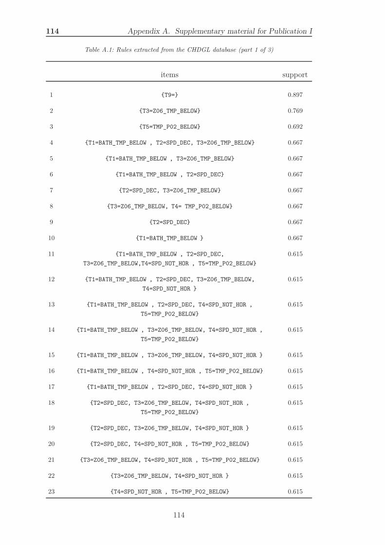
114 Appendix A. Supplementary material for Publication I
Table A.1: Rules extracted from the CHDGL database (part 1 of 3)
items support
1 {T9=} 0.897
2 {T3=Z06_TMP_BELOW} 0.769
3 {T5=TMP_P02_BELOW} 0.692
4 {T1=BATH_TMP_BELOW , T2=SPD_DEC, T3=Z06_TMP_BELOW} 0.667
5 {T1=BATH_TMP_BELOW , T3=Z06_TMP_BELOW} 0.667
6 {T1=BATH_TMP_BELOW , T2=SPD_DEC} 0.667
7 {T2=SPD_DEC, T3=Z06_TMP_BELOW} 0.667
8 {T3=Z06_TMP_BELOW, T4= TMP_P02_BELOW} 0.667
9 {T2=SPD_DEC} 0.667
10 {T1=BATH_TMP_BELOW } 0.667
11 {T1=BATH_TMP_BELOW , T2=SPD_DEC,
T3=Z06_TMP_BELOW,T4=SPD_NOT_HOR , T5=TMP_P02_BELOW}
0.615
12 {T1=BATH_TMP_BELOW , T2=SPD_DEC, T3=Z06_TMP_BELOW,
T4=SPD_NOT_HOR }
0.615
13 {T1=BATH_TMP_BELOW , T2=SPD_DEC, T4=SPD_NOT_HOR ,
T5=TMP_P02_BELOW}
0.615
14 {T1=BATH_TMP_BELOW , T3=Z06_TMP_BELOW, T4=SPD_NOT_HOR ,
T5=TMP_P02_BELOW}
0.615
15 {T1=BATH_TMP_BELOW , T3=Z06_TMP_BELOW, T4=SPD_NOT_HOR } 0.615
16 {T1=BATH_TMP_BELOW , T4=SPD_NOT_HOR , T5=TMP_P02_BELOW} 0.615
17 {T1=BATH_TMP_BELOW , T2=SPD_DEC, T4=SPD_NOT_HOR } 0.615
18 {T2=SPD_DEC, T3=Z06_TMP_BELOW, T4=SPD_NOT_HOR ,
T5=TMP_P02_BELOW}
0.615
19 {T2=SPD_DEC, T3=Z06_TMP_BELOW, T4=SPD_NOT_HOR } 0.615
20 {T2=SPD_DEC, T4=SPD_NOT_HOR , T5=TMP_P02_BELOW} 0.615
21 {T3=Z06_TMP_BELOW, T4=SPD_NOT_HOR , T5=TMP_P02_BELOW} 0.615
22 {T3=Z06_TMP_BELOW, T4=SPD_NOT_HOR } 0.615
23 {T4=SPD_NOT_HOR , T5=TMP_P02_BELOW} 0.615
114
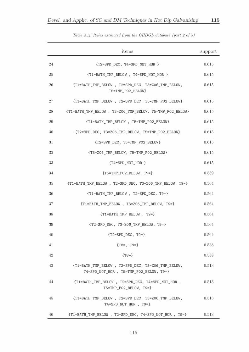
Devel. and Applic. of SC and DM Techniques in Hot Dip Galvanising 115
Table A.2: Rules extracted from the CHDGL database (part 2 of 3)
items support
24 {T2=SPD_DEC, T4=SPD_NOT_HOR } 0.615
25 {T1=BATH_TMP_BELOW , T4=SPD_NOT_HOR } 0.615
26 {T1=BATH_TMP_BELOW , T2=SPD_DEC, T3=Z06_TMP_BELOW,
T5=TMP_P02_BELOW}
0.615
27 {T1=BATH_TMP_BELOW , T2=SPD_DEC, T5=TMP_P02_BELOW} 0.615
28 {T1=BATH_TMP_BELOW , T3=Z06_TMP_BELOW, T5=TMP_P02_BELOW} 0.615
29 {T1=BATH_TMP_BELOW , T5=TMP_P02_BELOW} 0.615
30 {T2=SPD_DEC, T3=Z06_TMP_BELOW, T5=TMP_P02_BELOW} 0.615
31 {T2=SPD_DEC, T5=TMP_P02_BELOW} 0.615
32 {T3=Z06_TMP_BELOW, T5=TMP_P02_BELOW} 0.615
33 {T4=SPD_NOT_HOR } 0.615
34 {T5=TMP_P02_BELOW, T9=} 0.589
35 {T1=BATH_TMP_BELOW , T2=SPD_DEC, T3=Z06_TMP_BELOW, T9=} 0.564
36 {T1=BATH_TMP_BELOW , T2=SPD_DEC, T9=} 0.564
37 {T1=BATH_TMP_BELOW , T3=Z06_TMP_BELOW, T9=} 0.564
38 {T1=BATH_TMP_BELOW , T9=} 0.564
39 {T2=SPD_DEC, T3=Z06_TMP_BELOW, T9=} 0.564
40 {T2=SPD_DEC, T9=} 0.564
41 {T8=, T9=} 0.538
42 {T8=} 0.538
43 {T1=BATH_TMP_BELOW , T2=SPD_DEC, T3=Z06_TMP_BELOW,
T4=SPD_NOT_HOR , T5=TMP_P02_BELOW, T9=}
0.513
44 {T1=BATH_TMP_BELOW , T2=SPD_DEC, T4=SPD_NOT_HOR ,
T5=TMP_P02_BELOW, T9=}
0.513
45 {T1=BATH_TMP_BELOW , T2=SPD_DEC, T3=Z06_TMP_BELOW,
T4=SPD_NOT_HOR , T9=}
0.513
46 {T1=BATH_TMP_BELOW , T2=SPD_DEC, T4=SPD_NOT_HOR , T9=} 0.513
115

116 Appendix A. Supplementary material for Publication I
Table A.3: Rules extracted from the CHDGL database (part 3 of 3)
items support
47 {T1=BATH_TMP_BELOW , T3=Z06_TMP_BELOW, T4=SPD_NOT_HOR ,
T5=TMP_P02_BELOW, T9=}
0.513
48 {T1=BATH_TMP_BELOW , T4=SPD_NOT_HOR , T5=TMP_P02_BELOW,
T9=}
0.513
49 {T1=BATH_TMP_BELOW , T3=Z06_TMP_BELOW, T4=SPD_NOT_HOR ,
T9=}
0.513
50 {T1=BATH_TMP_BELOW , T4=SPD_NOT_HOR , T9=} 0.513
51 {T2=SPD_DEC, T3=Z06_TMP_BELOW, T4=SPD_NOT_HOR ,
T5=TMP_P02_BELOW, T9=}
0.513
52 {T2=SPD_DEC, T4=SPD_NOT_HOR , T5=TMP_P02_BELOW, T9=} 0.513
53 {T2=SPD_DEC, T3=Z06_TMP_BELOW, T4=SPD_NOT_HOR , T9=} 0.513
54 {T2=SPD_DEC, T4=SPD_NOT_HOR , T9=} 0.513
55 {T3=Z06_TMP_BELOW, T4=SPD_NOT_HOR , T5=TMP_P02_BELOW,
T9=}
0.513
56 {T4=SPD_NOT_HOR , T5=TMP_P02_BELOW, T9=} 0.513
57 {T3=Z06_TMP_BELOW, T4=SPD_NOT_HOR , T9=} 0.513
58 {T4=SPD_NOT_HOR , T9=} 0.513
59 {T1=BATH_TMP_BELOW , T2=SPD_DEC, T3=Z06_TMP_BELOW,
T5=TMP_P02_BELOW, T9=}
0.513
60 {T1=BATH_TMP_BELOW , T2=SPD_DEC, T5=TMP_P02_BELOW, T9=} 0.513
61 {T1=BATH_TMP_BELOW , T3=Z06_TMP_BELOW, T5=TMP_P02_BELOW,
T9=}
0.513
62 {T1=BATH_TMP_BELOW , T5=TMP_P02_BELOW, T9=} 0.513
63 {T2=SPD_DEC, T3=Z06_TMP_BELOW, T5=TMP_P02_BELOW, T9=} 0.513
64 {T2=SPD_DEC, T5=TMP_P02_BELOW, T9=} 0.513
116
Appendix B
Supplementary material for Publication II
B.1 Evolution of the attribute selection in THC3 and THC5
prediction models
The behaviour of the GAs selection carried out in the experiments for predicting
temperature THC1 was included in the paper as Figure 16 in (Sanz-García et al.,
2012). The rest of the experimental results obtained during THC3 and THC5
models´ optimisation was uploaded as Supplementary Material. For that reason,
processes of attribute selection for THC3 and THC5 prediction models are in-
cluded as Figure B.1 and Figure B.2, showing the percentage of ten best models
that included the input (vertical axis) via the number of generation (horizontal
axis).
117

118 Appendix B. Supplementary material for Publication II
0 5 10 15 20 25 30 35 40 45 49
050
100
CC
0 5 10 15 20 25 30 35 40 45 49
050
100
MnMn
0 5 10 15 20 25 30 35 40 45 49
050
100
SiSi
0 5 10 15 20 25 30 35 40 45 49
050
100
SS
0 5 10 15 20 25 30 35 40 45 49
050
100
PP
0 5 10 15 20 25 30 35 40 45 49
050
100
AlAl
0 5 10 15 20 25 30 35 40 45 49
050
100
CuCu
0 5 10 15 20 25 30 35 40 45 49
050
100
NiNi
0 5 10 15 20 25 30 35 40 45 49
050
100
CrCr
0 5 10 15 20 25 30 35 40 45 49
050
100
NbNb
0 5 10 15 20 25 30 35 40 45 49
050
100
VV
0 5 10 15 20 25 30 35 40 45 49
050
100
TiTi
0 5 10 15 20 25 30 35 40 45 49
050
100
BB
0 5 10 15 20 25 30 35 40 45 49
050
100
NN
0 5 10 15 20 25 30 35 40 45 49
050
100
ThickCoilThickCoil
0 5 10 15 20 25 30 35 40 45 49
050
100
WidthCoilWidthCoil
0 5 10 15 20 25 30 35 40 45 49
050
100
TMPP1TMPP1
0 5 10 15 20 25 30 35 40 45 49
050
100
TMPP2CNGTMPP2CNG
0 5 10 15 20 25 30 35 40 45 49
050
100
VelMedVelMed% Feature selectionwith complexity function
THC3
% Feature selectionwithout complexity function
THC3
Last Gen.
Last Gen.
Figure B.1: Evolution of attribute selection for all inputs in THC3 models
118
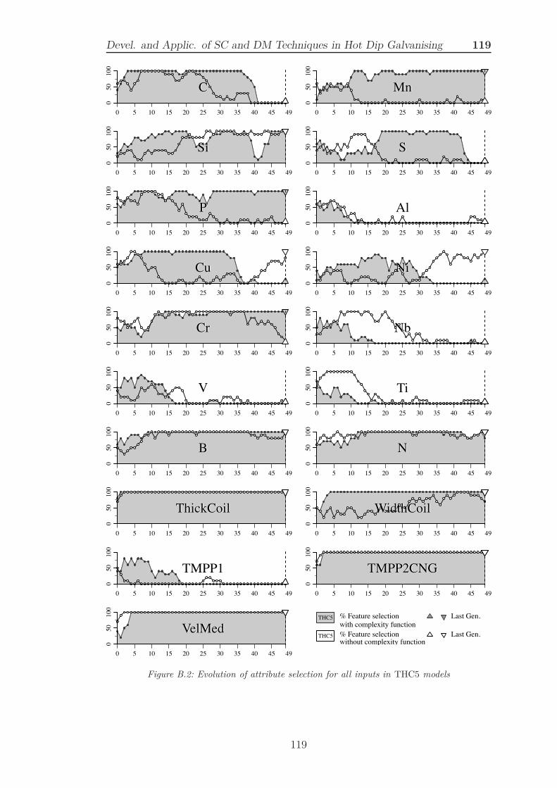
Devel. and Applic. of SC and DM Techniques in Hot Dip Galvanising 119
0 5 10 15 20 25 30 35 40 45 490
5010
0
CC
0 5 10 15 20 25 30 35 40 45 49
050
100
MnMn
0 5 10 15 20 25 30 35 40 45 49
050
100
SiSi
0 5 10 15 20 25 30 35 40 45 49
050
100
SS
0 5 10 15 20 25 30 35 40 45 49
050
100
PP
0 5 10 15 20 25 30 35 40 45 49
050
100
AlAl
0 5 10 15 20 25 30 35 40 45 49
050
100
CuCu
0 5 10 15 20 25 30 35 40 45 49
050
100
NiNi
0 5 10 15 20 25 30 35 40 45 49
050
100
CrCr
0 5 10 15 20 25 30 35 40 45 49
050
100
NbNb
0 5 10 15 20 25 30 35 40 45 49
050
100
VV
0 5 10 15 20 25 30 35 40 45 49
050
100
TiTi
0 5 10 15 20 25 30 35 40 45 49
050
100
BB
0 5 10 15 20 25 30 35 40 45 49
050
100
NN
0 5 10 15 20 25 30 35 40 45 49
050
100
ThickCoilThickCoil
0 5 10 15 20 25 30 35 40 45 49
050
100
WidthCoilWidthCoil
0 5 10 15 20 25 30 35 40 45 49
050
100
TMPP1TMPP1
0 5 10 15 20 25 30 35 40 45 49
050
100
TMPP2CNGTMPP2CNG
0 5 10 15 20 25 30 35 40 45 49
050
100
VelMedVelMed% Feature selectionwith complexity function
THC5
% Feature selectionwithout complexity function
THC5
Last Gen.
Last Gen.
Figure B.2: Evolution of attribute selection for all inputs in THC5 models
119

120 Appendix B. Supplementary material for Publication II
B.2 Figures for evaluating aggregation coefficients W
Figure 15 in (Sanz-García et al., 2012) shows the representation of validation and
testing RMSE via aggregation coefficient W for MLP networks developed during
50 generations. The range of the aggregation coefficients was cut at value W = 15.
The full range provides more information about the distribution of the different
values of complexity for all generations. Figure B.3, Figure B.4 and Figure B.5
show the RMSE values via processes aggregation coefficients W for temperature
THC1, THC3 and THC5 respectively. Black points represent validation and
grey points are testing data. The results of the prediction models developed with
complexity control are on the left side and without on the right side.
Root
Mea
n Sq
uare
d Er
ror (
RMSE
)
W
0 5 10 15 20 25 300.02
50.
050.
075
0.1
0.12
50.
15
Root
Mea
n Sq
uare
d Er
ror (
RMSE
)
W
0 5 10 15 20 25 300.02
50.
050.
075
0.1
0.12
50.
15
Figure B.3: Complete range of RMSE via aggregation coefficients W : THC1
Root
Mea
n Sq
uare
d Er
ror (
RMSE
)
W
0 5 10 15 20 25 300.02
50.
050.
075
0.1
0.12
50.
15
Root
Mea
n Sq
uare
d Er
ror (
RMSE
)
W
0 5 10 15 20 25 300.02
50.
050.
075
0.1
0.12
50.
15
Figure B.4: Complete range of RMSE via aggregation coefficients W : THC3
120
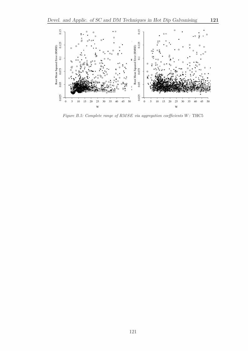
Devel. and Applic. of SC and DM Techniques in Hot Dip Galvanising 121
Root
Mea
n Sq
uare
d Er
ror (
RMSE
)
W
0 5 10 15 20 25 30 35 40 45 500.02
50.
050.
075
0.1
0.12
50.
15
Root
Mea
n Sq
uare
d Er
ror (
RMSE
)
W
0 5 10 15 20 25 30 35 40 45 500.02
50.
050.
075
0.1
0.12
50.
15
Figure B.5: Complete range of RMSE via aggregation coefficients W : THC5
121