development and application of models of chemical · pdf filedevelopment and application of...

Development and Application of Models of Chemical Fatein Canada

Practical Methods for Estimating Environmental Biodegradation Rates

Report to Environment Canada

CEMN Report No. 200503

Prepared by:

Jon Arnot, Todd Gouin, Don Mackay

Canadian Environmental Modelling NetworkTrent UniversityPeterborough, Ontario K9J 7B8 CANADA

Practical Methods for Estimating Environmental Biodegradation Rates

Jon Arnot Todd Gouin Don Mackay

Canadian Environmental Modelling Network Draft Guidance Report for Environment Canada in partial fulfillment of the Cooperative Agreement between Environment Canada and the Canadian Environmental Modelling

Network

March 31, 2005

ii

Executive Summary

Extensive research has been conducted towards understanding and estimating

biodegradation processes, yet for the vast majority of chemicals in commerce environmentally relevant biodegradation half-life values remain uncertain and difficult to access or estimate. The uncertainty in these rates is partially attributable to the observed natural variability resulting from different environmental conditions such as temperature, bioavailability and the genetic competence of microbial communities that may or may not be present. It is important to maximize the accuracy of chemical biodegradation rate data in the environment to minimize uncertainty associated with hazard and risk assessments. In this report a practical method for estimating biodegradation rates is described. It utilizes the inherent knowledge of the BIOWIN suite of biodegradation models. The models are calibrated to empirical aerobic environmental half-life data from 40 selected “training set” chemicals. The outcome of this calibration is compared to 115 “evaluation set” chemicals of environmental aerobic biodegradation. The calibrated BIOWIN estimation method is further compared with empirical half-life data and illustrative estimates from another biodegradation model (CATABOL). This evaluation reveals that the average absolute error is 116 and 2537 for the proposed method and CATABOL, respectively. The root mean square error is 279 and 5119 for the proposed method and CATABOL, respectively. This evaluation is not intended to be a direct model comparison since the revised BIOWIN predictions are a result of calibration to a subset of the evaluation set, whereas CATABOL is not. The potential application of the modified BIOWIN estimation method to a large number of chemical substances is investigated. A companion and more speculative method suggested in this report incorporates a “slide rule” approach for assessing all available empirical and estimated data for the biotransformation rate of a chemical.

1

Table of Contents

Executive Summary ii

Introduction 2

Sources of biodegradation data 2

Methods 4

Environmental aerobic biodegradation half-life estimation 4

Environmental biodegradation half-life estimation evaluation 5

General assessment of BIOWIN model output 5

Statistical analyses 6

Results and Discussion 6

Environmental aerobic biodegradation half-life estimation 6

Estimation method evaluation 6

General assessment of BIOWIN model output 7

A speculation on methods of improving the selection of biodegradation data 8

Conclusions 11

References 28

Appendix 30

2

Introduction

Chemicals in the environment are subject to processes such as transport (e.g., advection in a river), multimedia partitioning (e.g., air-water) and reaction (e.g., photolysis, hydrolysis and biodegradation). Chemical and biological reactions, or transformations, are the only mechanisms that alter and ultimately remove a chemical from the global environment. Biodegradation is the transformation of a chemical as a result of a living organism. All organisms including microorganisms, plants, insects and animals perform enzymatic chemical transformations. Generally, higher order organisms transform chemicals so that they can be more readily eliminated, whereas simpler organisms such as bacteria and fungi are responsible for most of the extensive biodegradation in the environment. Primary biodegradation changes the identity of the parent chemical as a first step to more extensive mineralisation, whereas ultimate biodegradation results in the complete mineralisation of the chemical to water, carbon dioxide and inorganic compounds [1]. Biodegradation is arguably one of the most important processes influencing the amount and persistence of chemical in the environment [2] but unfortunately the rates of these processes are poorly understood.

Multimedia models are used to provide quantitative understandings of the

environmental fate of chemicals and to assess potential risks to ecosystems and humans. Accurate media specific half-lives are essential for the reliable assessment of chemicals. Assuming first order kinetics the half-life t1/2 can be derived from a rate constant k as 0.693 / k. Fairly reliable methods are available for estimating the chemical half-life due to abiotic processes (e.g., [3]) but environmentally relevant biodegradation half-life information remains a major source of uncertainty [4]. Hazard assessment requires persistence data, which are dependent on the half-lives. Emissions and persistence control the mass and concentration of a chemical in the environment and hence the ultimate exposure and potential risk of a chemical. There is a need to improve existing methods of estimating environmental primary biodegradation half-lives to provide greater confidence in chemical assessments.

The objective of this report is to describe and evaluate pragmatic methods for

estimating environmentally relevant aerobic primary biodegradation half-lives as required for multimedia fate models. Two relatively simple and robust methods are described and evaluated. In the first method the inherent knowledge from four BIOWIN models is “calibrated” to empirical field-based half-life data. The ensuing predictions are then evaluated with empirical data and an example of other estimation methods (i.e., CATABOL). The potential for applying this method to a large number of chemicals, i.e., 10,600 organic chemicals, is investigated. The second, and more speculative, companion method describes a “slide-rule” approach that can be used to combine biotransformation information from all estimation sources and thus assess a substance’s inherent susceptibility to degradation in a more pictorial manner.

Sources of biodegradation data

Current sources of empirical biodegradation information include laboratory tests, field data, environmental handbooks and other databases. Standardized laboratory tests are

3

used to obtain empirical estimates of a chemical’s biodegradation potential. These include a suite of guideline tests recommended by the Organization for Economic Cooperation and Development (OECD). These tests are considered as standards for estimating the “ready” or “nonready” biodegradability of a substance. The protocols are not designed to provide an estimated rate for primary chemical transformation and the conditions employed are not relevant to environmental conditions. Extrapolation methods from laboratory tests have been suggested but these have been met with mixed reviews [5, 6]. Field studies (e.g., grab samples, river die-away) have been conducted for a few chemicals but such data are non-existent for most chemicals. Environmental handbooks (e.g, [7, 8]) provide collections of empirical data and can also provide guidelines for overall media specific half-lives. These sources provide compiled data and expert judgment, however they are generally limited in the scope of information they can offer for the vast number of chemicals used in commerce. Qualitative information is available for many biodegradation pathways most notably the University of Minnesota Biocatalysis/Biodegradation Database [2] and a Biodegradability Evaluation and Simulation System (BESS). Two other major sources of empirical information are the Syracuse Research Corporation’s BIODEG database, which contains over 5,800 records of experimental results on biodegradation studies for approximately 800 chemicals and the Japanese Ministry of International Trade and Industry (MITI) database. Most of these data are derived from laboratory studies. These databases have been used in model development but these models are not considered to be directly applicable for estimating environmentally relevant biodegradation rates for a large number of chemicals.

A variety of models has been developed to predict biodegradation. These include structure-biodegradability relationships (SBRs) and quantitative structure-biodegradability relationships (QSBRs). SBRs provide qualitative endpoints such as passing or failing a ready biodegradation test while QSBRs provide an estimation of rate or half-life. Examples of such models include BESS, BIOWIN, CATABOL, TOPKAT, and Multicase. Howard [1] and Jaworska et al [9] provide reviews for many of the different estimation methods currently available. These models are continually being refined and improved.

The Biodegradation Probability Program (BIOWIN) estimates the probability for the rapid biodegradation of an organic chemical in the presence of mixed populations of environmental microorganisms [10-14]. BIOWIN was developed by the Syracuse Research Corporation (SRC) and the US EPA as part of the EPIWIN/EPISUITE™ model package and is freely available from the US EPA website [15]. BIOWIN includes six different models including: (1) linear probability BIODEG, (2) nonlinear probability BIODEG, (3) expert survey ultimate biodegradation model (USM), (4) expert survey primary biodegradation model (PSM), (5) Japanese MITI linear, and (6) Japanese MITI nonlinear. These are generally referred to as BIOWIN1_6. Estimates are based on fragment constants and molecular weight and require only a chemical structure. These models have been developed and tested for a range of chemical substances for assessing the biodegradation potential of chemicals by regulatory agencies.

The BIOWIN models have been developed to screen and classify chemical

biodegradability (i.e., ready and nonready). The expert survey models (BIOWIN3_4) provide estimates for the time required to achieve primary and ultimate aerobic biodegradation in water. Boethling et al have provided recommendations for converting this

4

information to environmental half-lives, however they suggest that these estimates not be used as inputs for multimedia modelling assessments [16]. The BIOWIN models include significant inherent information on the relative biodegradability of chemicals derived from different sources (i.e., SRC and MITI empirical data sets and expert judgment). If this knowledge could be adapted to empirical and estimated field based measures of primary biodegradation half-lives then perhaps the utility of the BIOWIN models could be extended.

Methods

Environmental aerobic biodegradation half-life estimation

In an attempt to develop a pragmatic method of selecting biodegradation half-lives for regulatory assessment purposes, a total of 40 chemicals were selected as a “training set” for the calibration of BIOWIN models 1, 3, 4, 5 (i.e., linear BIODEG, USM, PSM and linear MITI) to reliable assessments of aerobic biodegradation environmental half-lives. The 40 chemicals were selected based on the availability of reliable measurements (i.e., sample size). Chemical and structural diversity were included to the greatest extent possible. Data were compiled from handbooks [7, 8], the Syracuse Research Corporation BIODEG database and the primary literature. Primary research sources were obtained and the data evaluated for quality. The selected empirical data were largely aqueous aerobic half-lives although some values were estimated from soil based studies (i.e., [7]). These half-life values for soil were included if it was observed that they were in the range of aqueous data. Only those half-lives interpreted as being primary biodegradation rates were considered. Table 1 provides a list of the 40 chemical “training set” and summary statistics of the empirical environmental half-lives. Figure 1 illustrates the log normal distribution of half-lives considered for the calibration. Appendix 1 includes further information on the physical-chemical properties and illustrates the range of chemical structures included in this compilation.

Raw numerical output from each of the four BIOWIN models was generated for the 40 chemicals. The raw output for each model was then calibrated by linear regression to the corresponding arithmetic means from the empirical biodegradation half-lives. The arithmetic mean was selected as a metric for calibration rather than the geometric mean because there are generally few observations for each chemical with many exhibiting a wide range in half-lives. Given the uncertainty in measurement and the variability associated with environmental half-lives it was decided to calibrate to a higher average to provide a modest degree of conservatism.

If a value for biodegradation was reported as the %BOD (Biochemical Oxygen

Demand) or as the percentage of chemical degraded then this information was converted to a half-life estimate. Assuming first order decay from an initial quantity C0 to C in time t gives:

C = C0 exp(−kt) (1)

5

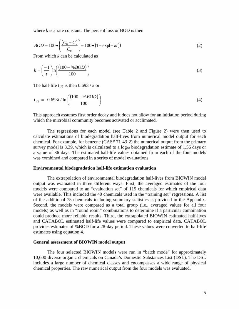
where k is a rate constant. The percent loss or BOD is then

( ) ( )( )ktC

CCBOD −−•=⎟⎟⎠

⎞⎜⎜⎝

⎛ −•= exp1100100

0

0 (2)

From which k can be calculated as

( )⎟⎠⎞

⎜⎝⎛ −

⎟⎠⎞

⎜⎝⎛ −=

100%100ln1 BOD

tk (3)

The half-life t1/2 is then 0.693 / k or

( )⎟⎠⎞

⎜⎝⎛ −

=100%100ln0.693t / - t1/2

BOD (4)

This approach assumes first order decay and it does not allow for an initiation period during which the microbial community becomes activated or acclimated.

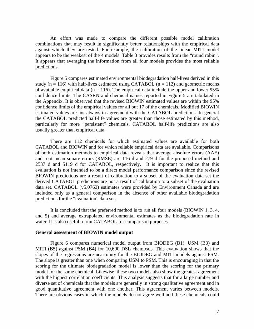
The regressions for each model (see Table 2 and Figure 2) were then used to calculate estimations of biodegradation half-lives from numerical model output for each chemical. For example, for benzene (CAS# 71-43-2) the numerical output from the primary survey model is 3.39, which is calculated to a log10 biodegradation estimate of 1.56 days or a value of 36 days. The estimated half-life values obtained from each of the four models was combined and compared in a series of model evaluations.

Environmental biodegradation half-life estimation evaluation

The extrapolation of environmental biodegradation half-lives from BIOWIN model output was evaluated in three different ways. First, the averaged estimates of the four models were compared to an “evaluation set” of 115 chemicals for which empirical data were available. This included the 40 chemicals used in the “training set” regressions. A list of the additional 75 chemicals including summary statistics is provided in the Appendix. Second, the models were compared as a total group (i.e., averaged values for all four models) as well as in “round robin” combinations to determine if a particular combination could produce more reliable results. Third, the extrapolated BIOWIN estimated half-lives and CATABOL estimated half-life values were compared to empirical data. CATABOL provides estimates of %BOD for a 28-day period. These values were converted to half-life estimates using equation 4.

General assessment of BIOWIN model output

The four selected BIOWIN models were run in “batch mode” for approximately 10,600 diverse organic chemicals on Canada’s Domestic Substances List (DSL). The DSL includes a large number of chemical classes and encompasses a wide range of physical chemical properties. The raw numerical output from the four models was evaluated.

6

Statistical analyses

Statistical analyses were conducted using Microsoft EXCEL™ and JMPIN™ (SAS institute).

Results and Discussion

Environmental aerobic biodegradation half-life estimation

The series of plots in Figure 2 illustrates the calibration of BIOWIN model output to 40 selected “training set” chemicals. The empirical half-lives are the arithmetic mean for each chemical and are plotted on a logarithmic scale. These calibrations indicate a good correlation between the empirical data and the model predictions. For these 40 chemicals the relationship is strongest for the survey models followed by the linear BIODEG model and the linear MITI model. Table 2 summarizes the resulting equations and statistics for each regression. Restrictions were applied to low values of model output. For example, if PSM output was less than 2 the chemical was considered to have a maximum half-life of 3650 days (10 years). Likewise, a USM output less than 0.85 corresponds to a maximum half-life of 2190 days (6 years), linear BIODEG output less than -0.95 corresponds to 3300 days (~9 years) and linear MITI output less than -0.7 corresponds to 3650 days (10 years). The purpose of this calibration is to provide a means to estimate “real world” biodegradation half-lives for application in multimedia fate models. The aim is not provide accurate biodegradation rates for extremely recalcitrant chemicals. For the purposes of multimedia fate modelling there is a point at which low biodegradation rates become relatively less important in comparison to other processes such as advective losses.

These equations provide an estimate of aerobic environmental half-life (i.e., y) from

the output of each BIOWIN model (i.e., x). The regression equations provide the log10 biodegradation environmental half-lives. The estimated environmental biodegradation half-lives were averaged in an effort to obtain “balance” between model errors. The models could be used to produce either an arithmetic mean or a geometric mean. The coefficient of variation could be used to identify the relative agreement or disagreement between the four models. Professional judgment could also be used to remove a particular model prediction that does not follow a pattern identified by the other models (i.e., an extreme value).

Estimation method evaluation

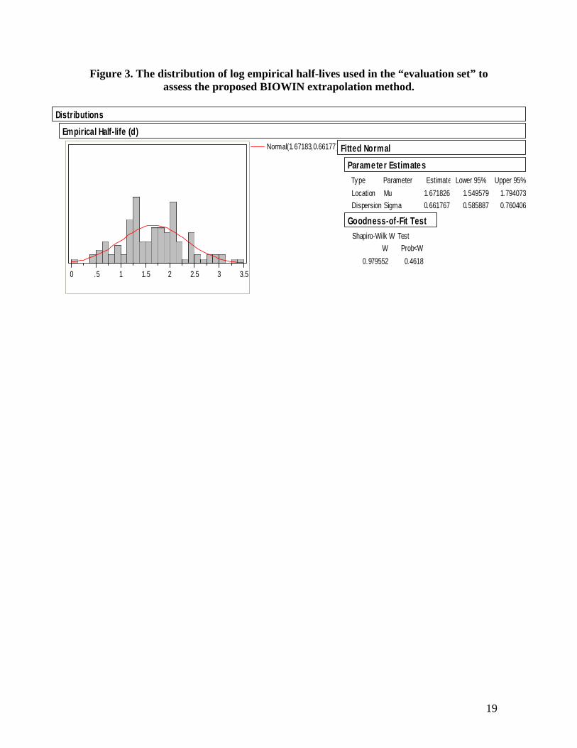
The estimated environmental half-lives were evaluated in comparison to empirical data and to other model estimates. Figure 3 illustrates the log-normal distribution of empirical half-life values from the “evaluation set” of 115 chemicals. This indicates that a wide range of empirical half-life information was included for the evaluation. Figure 4 compares aerobic biodegradation half-lives using the arithmetic mean from half-life estimates from all four models with empirical data for 115 chemicals. Using this approach 98% and 77% of the 115 chemicals are predicted within a factor of 10 and a factor of 3 of the empirical data, respectively. Those values that lie outside a factor of 10 are all conservative model predictions. For screening level assessments conservative errors are preferable.

7

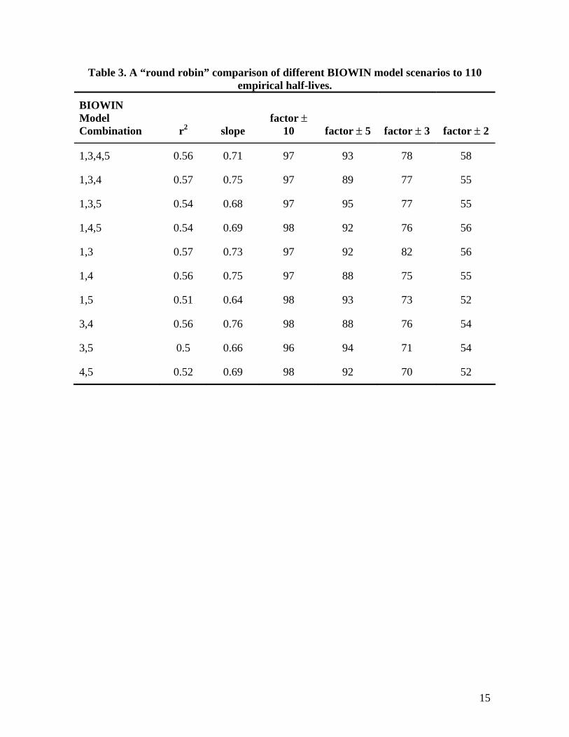
An effort was made to compare the different possible model calibration

combinations that may result in significantly better relationships with the empirical data against which they are tested. For example, the calibration of the linear MITI model appears to be the weakest of the 4 models. Table 3 provides results from the “round robin”. It appears that averaging the information from all four models provides the most reliable predictions.

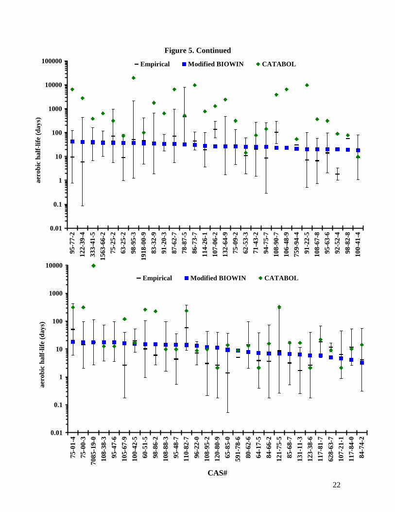
Figure 5 compares estimated environmental biodegradation half-lives derived in this study (n = 116) with half-lives estimated using CATABOL (n = 112) and geometric means of available empirical data (n = 116). The empirical data include the upper and lower 95% confidence limits. The CASRN and chemical names reported in Figure 5 are tabulated in the Appendix. It is observed that the revised BIOWIN estimated values are within the 95% confidence limits of the empirical values for all but 17 of the chemicals. Modified BIOWIN estimated values are not always in agreement with the CATABOL predictions. In general the CATABOL predicted half-life values are greater than those estimated by this method, particularly for more “persistent” chemicals. CATABOL half-life predictions are also usually greater than empirical data.

There are 112 chemicals for which estimated values are available for both

CATABOL and BIOWIN and for which reliable empirical data are available. Comparisons of both estimation methods to empirical data reveals that average absolute errors (AAE) and root mean square errors (RMSE) are 116 d and 279 d for the proposed method and 2537 d and 5119 d for CATABOL, respectively. It is important to realize that this evaluation is not intended to be a direct model performance comparison since the revised BIOWIN predictions are a result of calibration to a subset of the evaluation data set the derived CATABOL predictions are not a result of calibration to a subset of the evaluation data set. CATABOL (v5.0763) estimates were provided by Environment Canada and are included only as a general comparison in the absence of other available biodegradation predictions for the “evaluation” data set.

It is concluded that the preferred method is to run all four models (BIOWIN 1, 3, 4,

and 5) and average extrapolated environmental estimates as the biodegradation rate in water. It is also useful to run CATABOL for comparison purposes.

General assessment of BIOWIN model output

Figure 6 compares numerical model output from BIODEG (B1), USM (B3) and MITI (B5) against PSM (B4) for 10,600 DSL chemicals. This evaluation shows that the slopes of the regressions are near unity for the BIODEG and MITI models against PSM. The slope is greater than one when comparing USM to PSM. This is encouraging in that the scoring for the ultimate biodegradation model is lower than the scoring for the primary model for the same chemical. Likewise, these two models also show the greatest agreement with the highest correlation coefficients. This analysis suggests that for a large number and diverse set of chemicals that the models are generally in strong qualitative agreement and in good quantitative agreement with one another. This agreement varies between models. There are obvious cases in which the models do not agree well and these chemicals could

8

be investigated to have a better understanding as to why these differences exist and how such differences can be corrected or minimized. More importantly, addressing these differences may identify aspects of the models that could be improved.

Residuals from the model correlations tend to increase for predictions of “more persistent” chemicals, i.e., longer half-lives. One explanation for this is that the survey models are “more accurate” for relatively more biodegradable chemicals compared to less biodegradable chemicals as a result of their design. For example, the survey asked experts to assign a value of 5, 4, 3, 2, or 1 corresponding to general time categories of either primary or ultimate aerobic biodegradation in the environment. These categories are “hours”, “days”, “weeks”, “months” or “longer”. Provided with this scale for classification an expert would likely interpret “hours” as less than or equal to approximately 1 day, whereas months would perhaps have been interpreted as 60 to 365 days. It is difficult to quantify the “longer” category. Clearly, the associated errors and uncertainties in assigning a number to these qualitative descriptors will increase with increasing temporal scale. This is unfortunate because a major regulatory effort is to identify, evaluate and possibly regulate persistent chemicals in the environment. Although this expert knowledge is difficult to obtain and is subjective, a more quantitatively explicit survey in the future could result in reduced uncertainty for developing environmental half-life models for both primary and ultimate biodegradation.

Figure 7 illustrates the distributions of model output from the four BIOWIN models

for 10,600 substances. This evaluation provides a reasonable assessment for the range of possible model outputs that can be expected for organic chemicals. These distributions suggest that the “extreme” model predictions are generally observed for “more persistent” chemicals. Figure 8 indicates that extreme model output is largely associated with increasing molecular weight. This can be interpreted as a “residual effect” of the contribution method for larger chemicals. It may also reflect the lower solubility in water and hence availability of these substances. This has also been observed for physical-chemical property estimations when applying EPIWIN and other contribution models to high molecular weight chemicals. This preliminary analysis identifies extreme BIOWIN model outputs and suggests careful analysis of the results for chemicals with molecular weight greater than approximately 500. This information also suggests that there are possible limiting values for each model that should be restricted.

A speculation on methods of improving the selection of biodegradation data

The objective of this section is to speculate on methods that may be developed in the future and to display empirical and estimate biodegradation rate data leading to an optimal selection of half-lives for various environmental compartments.

First it is useful to set an ultimate target in terms of accuracy for these estimates.

Rather than give actual numerical estimates of half-lives, e.g., 100 hours, it is probably more honest to assign a chemical to a “bin” or half-life range of say 50 to 200 hours. The “width” of these bins can be varied according to the perceived accuracy. Mackay et al [8] have suggested that these bins could be “semi-decade” wide, i.e., factor of approximately 3

9

from low to high end. For abiotic reactions such as atmospheric oxidation and hydrolysis this is certainly achievable, but it is currently optimistic for biodegradation kinetics.

The semi-decade or factor of 3 level of discrimination is a compromise between

conveying an exaggerated impression of accuracy (as would be implied by a factor of 2 range) and a rather pessimistic use of factor of 10 ranges. In many cases the rates are known with error limits of factor of 2 or 3. Half-life data can be obtained from field tests, STP treatability, QSARs and expert judgment. Obviously the results from each source will differ, for example the following is a hypothetical list.

Source Half-life (hours) Metabolism in rat 20 Sewage treatment plant (STP) 40 BOD test 100 Water test (e.g., river die away) 300 Soil test 600 Sediment test or expert judgment 1000 QSAR1 200 QSAR2 500 QSAR3 120

These different quantities represent different “currencies” but they all refer to

biodegradation phenomena, albeit in different environments at different conditions and probably with different microbial systems. If a large database can be compiled it may be possible to develop relationships between, for example, typical STP half-lives and water or soil half-lives. A difficulty is that x, y correlations can only be done on two quantities at a time. It would be useful if a correlation or multiple regression approach could be devised in which all the data are treated simultaneously. It is suggested that this can be done using a “slide rule” approach in which the logarithmic half-life scales are displaced by an amount corresponding to the slope of the x, y plot on a logarithmic basis. The slope is essentially a factor.

It is useful to review briefly the principle of the slide rule. Regrettably, slide rules,

which were once standard equipment for the engineer, are now virtually obsolete. Two logarithmic scales can be slid past each other or displaced to a desired extent. To multiply 2 by 3 the point 1.0 on the mobile slide is set at 2.0 on the stationary scale and the answer (6.0) is read off on the slide opposite 3.0 on the slide, Effectively log 2 is added to log 3 to give log 6.

In this case each biodegradation data source is an individual slide rule marked in classes as shown in Figure 9. The relative data source to data source adjustment is obtained by correlation of log half-life versus log half-life (t) forcing a parameter correlation of the type log t1 = A + log t2 (5)

10

This is equivalent to t1 = 10A t2 (6)

An even simpler correlation is to force A to adopt one of several positive or negative values such as 0.5, 1.0, 2.0, -0.5, -1.5 etc. where n is a positive or negative integer. This essentially relates the half-life ranges to each other rather than the numerical values. The factors 10A then adopt values such as 3.1, 10, 31, 0.31, and 0.1 i.e., 100.5n where n in these examples is 1, 2, 3, -1, and -2.

Figure 9 gives a fictitious result for a "persistent" and a "non-persistent" substance in which the correlations have been fairly successful and take the form of displacement by the specified number of ranges. It is not expected that it will be possible to align all the ranges for all substances but the diagram has the potential to convey an impression of persistence, to assess the consistency between data inputs (or more strictly test if they fit the correlation implied by the specified displacement) and in the absence of any experimental data they enable QSAR data to be used to estimate the ranges in which other half-lives are likely to lie. Using ranges avoids conveying an impression of excessive accuracy. The user is at liberty to select single numerical half-lives from the range, but that selection is clearly the responsibility of the user.

In order to construct the slide rule a quantity of reliable biodegradation data should

be gathered and correlations sought between the various sources. Pairs of sources are compared and mean factors relating the half-lives are established. For example, soil half-life is 3 times the water half-life value on average. Some of these factors are subject to varying accuracy. From the matrix of pairs of factors a single set is established and used to set the slide rules. If the factors apply to a specific chemical, the classes will be aligned horizontally, but it is expected that there will be deviations. If the method has validity the data should lied generally on a horizontal band, the location of which indicates the biodegradability. This has the advantage that the output is pictorial rather than numerical and the results may be more readily understood.

Inherent in this approach is the assumption that the biodegradation process is

fundamentally second order in nature, specifically first order with respect to the chemical and first order with respect to the microbial community that prevails in that compartment.

It is recommended that this approach be explored by applying it to a set of

biodegradation data for chemicals in a variety of media. The usefulness of the method can only be evaluated in the light of experience.

11

Conclusions

From this analysis it is suggested that for DSL chemicals the most reliable and robust approach is to

(1) Gather all available empirical data for the substance of interest in all relevant

media. (2) Run the four BIOWIN models (1, 3, 4, and 5) and the CATABOL model,

average the BIOWIN half-lives and check that the results are generally consistent with the CATABOL results.

(3) The empirical and model data are then combined using expert judgment to suggest a range of half-lives which may be applicable to that substance.

(4) Apply factors to relate water, soil, and sediment half-lives and possibly STP half-lives. This can be done directly or using the slide rule pictorial approach.

It is recommended that the feasibility and usefulness of the slide rule approach be evaluated in a companion study.

12

Table 1. A list and statistical summary of empirical aerobic environmental half-lives for 40 chemicals selected as a “training set” to calibrate the BIOWIN models.

Empirical t1/2 (d) log

CAS Chemical Name n Arithmetic mean STDEV CV Mean

71-43-2 Benzene 8 40 46 1.15 1.60

84-66-2 Diethylphthalate (DEP) 7 11 20 1.86 1.03

87-86-5 Pentachlorophenol 7 146 183 1.25 2.16

93-76-5 2,4,5-trichlorophenoxyacetic acid 7 25 18 0.73 1.40

108-95-2 Phenol 6 5 4 0.83 0.70

1912-24-9 Atrazine 7 96 71 0.74 1.98

85-68-7 Butyl benzyl phthalate (BBP) 6 4 4 0.85 0.64

100-41-4 Ethylbenzene 6 14 13 0.92 1.15

106-44-5 p-cresol 5 1 1 0.95 0.10

58-89-9 γ-HCH (lindane) 5 392 299 0.76 2.59

63-25-2 Carbaryl 5 14 12 0.86 1.14

76-44-8 Heptachlor 5 824 1074 1.30 2.92

91-20-3 Naphthalene 5 40 17 0.42 1.60

91-22-5 Quinoline 4 14 18 1.30 1.14

95-95-4 2,4,5-trichlorophenol 4 366 360 0.98 2.56

116-06-3 Aldicarb 5 131 165 1.26 2.12

118-74-1 Hexachlorobenzene 5 1245 850 0.68 3.10

122-34-9 Simazine 5 81 52 0.64 1.91

131-11-3 Dimethylphthalate (DMP) 5 3 3 1.04 0.40

1563-66-2 Carbofuran 5 40 26 0.65 1.60

1746-01-6 2,3,7,8-TCDD 5 648 247 0.38 2.81

1918-00-9 Dicamba 5 69 66 0.96 1.84

13


CAS Chemical Name n Arithmetic mean STDEV CV Mean

50-32-8 Benzo[a]pyrene 4 284 201 0.71 2.45

56-55-3 Benz[a]anthracene 4 301 261 0.87 2.48

72-43-5 Methoxychlor 4 191 147 0.77 2.28

75-01-4 Chloroethene (vinyl chloride) 4 76 75 0.98 1.88

108-60-1 Bis(2-chloroisopropyl)ether 4 66 80 1.21 1.82

108-88-3 Toluene 4 18 16 0.89 1.26

120-82-1 1,2,4-trichlorobenzene 4 61 79 1.30 1.79

121-14-2 2,4-dinitrotoluene 2 104 107 1.03 2.02

206-44-0 Fluoranthene 4 306 132 0.43 2.49

7085-19-0 Mecoprop 4 25 24 1.00 1.39

64-17-5 Ethanol 3 5 4 0.72 0.73

65-85-0 Benzoic acid 3 2 2 0.80 0.39

91-94-1 3,3'-dichlorobenzidine 3 93 78 0.83 1.97

98-86-2 Acetophenone 2 6 2 0.40 0.80

106-42-3 p-xylene (Benzene, 1,4-dimethyl-) 3 19 11 0.57 1.29

107-21-1 Ethylene glycol 3 8 5 0.66 0.92

108-67-8 1,3,5-trimethylbenzene 3 9 8 0.87 0.97

120-80-9 Catechol 2 4 4 1.06 0.60

14

Table 2. General equations used to derive estimates of aerobic environmental biodegradation half-lives from BIOWIN model output. These do not include suggested

“restrictions” for the low numerical output of chemicals that are modeled to be very persistent.

BIOWIN Model Regression Equation r2

B1 - linear BIODEG y = -1.32x + 2.24 0.72

B3 - USM y = -1.07x + 4.20 0.77

B4 - PSM y = -1.46x + 6.51 0.78

B5 - linear MITI y = -1.86x + 2.23 0.58

15

Table 3. A “round robin” comparison of different BIOWIN model scenarios to 110 empirical half-lives.

BIOWIN Model Combination r2 slope

factor ± 10 factor ± 5 factor ± 3 factor ± 2

1,3,4,5 0.56 0.71 97 93 78 58

1,3,4 0.57 0.75 97 89 77 55

1,3,5 0.54 0.68 97 95 77 55

1,4,5 0.54 0.69 98 92 76 56

1,3 0.57 0.73 97 92 82 56

1,4 0.56 0.75 97 88 75 55

1,5 0.51 0.64 98 93 73 52

3,4 0.56 0.76 98 88 76 54

3,5 0.5 0.66 96 94 71 54

4,5 0.52 0.69 98 92 70 52

16

Figure 1. The distribution of log transformed empirical biodegradation half-lives for 40 chemicals used as a “training set” to calibrate the BIOWIN models.

0 .5 1 1.5 2 2.5 3 3.5

Normal(1.6005,0.76554)

LocationDispersion

Ty peMuSigma

Parameter 1.600500 0.765543

Estimate 1.355667 0.627103

Lower 95% 1.845333 0.982984

Upper 95%

Paramete r Estimates

Shapiro-Wilk W Test

0.974044W

0.5944Prob<W

Goodness-of-Fit Tes t

Fitted Normallog half-life (d)

Distributions

17

Figure 2. Log-linear regressions of BIOWIN model output to empirical aerobic half-life data and equations used to extrapolate “environmentally relevant” aerobic half-

life data. BIOWIN - BIODEG (B1)

y = -1.32x + 2.24r2 = 0.72

0

0.5

1

1.5

2

2.5

3

3.5

-1 -0.5 0 0.5 1 1.5

Raw model output

log

empi

rica

l aer

obic

hal

f-lif

e (d

)

BIOWIN - Ultimate Survey Model (USM-B3)

y = -1.07x + 4.12r2 = 0.77

0

0.5

1

1.5

2

2.5

3

3.5

4

0 1 2 3 4

Raw model output

log

empi

rica

l aer

obic

hal

f-lif

e (d

)

18

Figure 2. Continued

BIOWIN - Primary Survey Model (PSM-B4)

y = -1.46x + 6.51r2 = 0.78

0

0.5

1

1.5

2

2.5

3

3.5

4

1 2 3 4 5

Raw model output

log

empi

rica

l aer

obic

hal

f-lif

e (d

)

BIOWIN - MITI (B5)

y = -1.86x + 2.23r2 = 0.58

0

0.5

1

1.5

2

2.5

3

3.5

-1 -0.5 0 0.5 1 1.5

Raw model output

log

empi

rica

l aer

obic

hal

f-lif

e (d

)

19

Figure 3. The distribution of log empirical half-lives used in the “evaluation set” to assess the proposed BIOWIN extrapolation method.

0 .5 1 1.5 2 2.5 3 3.5

Normal(1.67183,0.66177)

LocationDispersion

TypeMuSigma

Parameter 1.671826 0.661767

Estimate 1.549579 0.585887

Lower 95% 1.794073 0.760406

Upper 95%

Parameter Estimates

Shapiro-Wilk W Test

0.979552W

0.4618Prob<W

Goodness-of-Fit Test

Fitted NormalEmpirical Half-life (d)

Distributions

20

Figure 4. A comparison of estimated half-lives using the average calibrated output from the four BIOWIN models and empirical aerobic biodegradation half-lives. The

black line represents a 1:1 ratio and the gray lines represent ± factors of 3 and 10.

y = 0.73x + 0.49r2 = 0.57

-1

0

1

2

3

4

-1 0 1 2 3 4

log aerobic empirical half-life (d)

log

aero

bic

aver

age

BIO

WIN

hal

f-lif

e (d

)

21

Figure 5. Estimated biodegradation half-lives from the modified BIOWIN models, CATABOL and available empirical data. (error bars represent the 95% CL)

0.1

1

10

100

1000

10000

10000072

-20-

811

5-29

-715

82-0

9-8

118-

74-1

67-7

2-1

3382

0-53

-077

-47-

491

-94-

187

-86-

558

-89-

932

598-

13-3

3569

3-99

-372

-55-

919

1-24

-218

97-4

5-6

2303

-17-

521

725-

46-2

207-

08-9

50-3

2-8

1746

-01-

621

8-01

-956

-55-

313

3-06

-219

12-2

4-9

72-4

3-5

2921

-88-

212

9-00

-020

6-44

-058

-90-

2

aero

bic

half-

life

(day

s)

Empirical Modified BIOWIN CATABOL

0.1

1

10

100

1000

10000

100000

3768

0-65

-212

1-14

-212

2-34

-923

03-1

6-4

56-2

3-5

330-

55-2

120-

82-1

79-3

4-5

330-

54-1

95-9

5-4

88-0

6-2

122-

14-5

127-

18-4

298-

00-0

75-6

9-4

86-3

0-6

56-3

8-2

108-

60-1

314-

40-9

111-

44-4

106-

46-7

96-1

8-4

120-

12-7

85-0

1-8

116-

06-3

79-0

1-6

93-7

6-5

67-6

6-3

120-

83-2

CAS#

aero

bic

half-

life

(day

s)


22

Figure 5. Continued

0.01

0.1

1

10

100

1000

10000

75-0

1-4

75-0

0-3

7085

-19-

010

8-38

-395

-47-

610

5-67

-910

0-42

-560

-51-

598

-86-

210

8-88

-395

-48-

711

0-82

-796

-22-

010

8-95

-212

0-80

-965

-85-

059

1-78

-680

-62-

664

-17-

584

-66-

212

1-75

-585

-68-

713

1-11

-312

3-38

-611

7-81

-762

8-63

-710

7-21

-111

7-84

-084

-74-

2

CAS#

aero

bic

half-

life

(day

s)


0.01

0.1

1

10

100

1000

10000

10000095

-77-

212

2-39

-433

3-41

-515

63-6

6-2

75-2

5-2

63-2

5-2

98-9

5-3

1918

-00-

983

-32-

991

-20-

387

-62-

778

-87-

586

-73-

711

4-26

-110

7-06

-213

2-64

-975

-09-

262

-53-

371

-43-

294

-75-

710

8-90

-710

6-48

-975

9-94

-491

-22-

510

8-67

-895

-63-

692

-52-

498

-82-

810

0-41

-4

aero

bic

half-

life

(day

s)


23

Figure 6. Numerical output comparisons of BIOWIN models for 10,600 diverse chemicals.

y = 0.8847x - 2.5519r2 = 0.6448

-6

-4

-2

0

2

4

-2 0 2 4 6

PSM (B4) numerical output

BIO

DE

G (B

1) n

umer

ical

out

put

y = 0.9977x - 3.2602r2 = 0.6777

-6

-4

-2

0

2

4

-2 0 2 4 6


MIT

I (B

5) n

umer

ical

out

put

24

Figure 6. Continued

y = 1.3472x - 2.2034r2 = 0.8828

-6

-4

-2

0

2

4

6

-2 0 2 4 6


USM

(B3)

num

eric

al o

utpu

t

25

Figure 7. Distributions of BIOWN 1, 3, 4, 5 output for organic chemicals on the DSL.

-4 -3 -2 -1 0 1 2 3

100.0%99.5%97.5%90.0%75.0%50.0%25.0%10.0%2.5%0.5%0.0%

maximum

quartilemedianquartile

minimum

2.9040 1.5727 1.2157 1.0266 0.8753 0.6751 0.2901-0.1759-1.1484-2.2458-4.5759

QuantilesMeanStd DevStd Err Meanupper 95% Meanlower 95% MeanN

0.51222720.59943400.00581290.52362180.5008326

10634

Momentslinear BIODEG (B1) 2

-5 -4 -3 -2 -1 0 1 2 3 4

100.0%99.5%97.5%90.0%75.0%50.0%25.0%10.0%2.5%0.5%0.0%

maximum


minimum

4.1039 3.6563 3.4171 3.1803 2.9515 2.6979 2.1693 1.3605 0.4281-0.6817-5.5569


2.462558 0.780079 0.007565 2.477386 2.447729 10634

MomentsUSM (B3)

-1 0 1 2 3 4 5

100.0%99.5%97.5%90.0%75.0%50.0%25.0%10.0%2.5%0.5%0.0%

maximum


minimum

5.0064 4.5174 4.2802 4.0366 3.8064 3.5720 3.2273 2.7182 2.1403 1.4594-1.5915


3.463470 0.544061 0.005276 3.473812 3.453128 10634

MomentsPSM (B4)

-5 -4 -3 -2 -1 0 1 2 3

100.0%99.5%97.5%90.0%75.0%50.0%25.0%10.0%2.5%0.5%0.0%

maximum


minimum

2.7776 1.3315 1.0289 0.8061 0.6111 0.3678-0.0526-0.6612-1.6203-2.4769-5.1378


0.19521890.65935690.00639400.20775260.1826852

10634

Momentslinear MITI (B5)

Distributions

Figure 8. A plot of the residuals of BIOWIN model output against molecular weight.

26

-5-4-3-2-101234

USM

(B3)

0 200 400 600 800 1000 1300 1600 1900MW

Linear Fit

USM (B3) = 3.3435193 - 0.0027961 MW

RSquareRSquare AdjRoot Mean Square ErrorMean of ResponseObservations (or Sum Wgts)

0.6451640.645131 0.4647

2.462558 10634

Summary of Fit

-4.0

-2.0

0.0

2.0

4.0

Res

idua

l0 100 300 500 700 900 1100 1300 1500 1700 1900 2100

MW

Linear Fit

Bivariate Fit of USM (B3) By MW

-1

0

1

2

3

4

5

PSM

(B4)

0 200 400 600 800 1000 1300 1600 1900MW

Linear Fit

PSM (B4) = 3.9801803 - 0.00164 MW


0.456280.4562290.401195 3.46347 10634

Summary of Fit

-3-2

0

2

Res

idua

l

0 100 300 500 700 900 1100 1300 1500 1700 1900 2100MW

Linear Fit

Bivariate Fit of PSM (B4) By MW

-4

-3

-2

-1

0

1

2

3

linea

r BI

OD

EG (B

1)

0 200 400 600 800 1000 1300 1600 1900MW

Linear Fit

linear BIODEG (B1) = 1.00557 - 0.0015658 MW


0.3426480.3425860.4860280.512227 10634

Summary of Fit

-3

-1

1

3

Res

idua

l

0 100 300 500 700 900 1100 1300 1500 1700 1900 2100MW

Linear Fit

Bivariate Fit of linear BIODEG (B1) By MW

-5

-4

-3

-2

-1

0

1

2

3

linea

r M

ITI (

B5)

0 200 400 600 800 1000 1300 1600 1900MW

Linear Fit

linear MITI (B5) = 0.8889479 - 0.0022019 MW


0.5599790.5599370.4373990.195219 10634

Summary of Fit

-2.0

0.0

2.0

4.0

6.0

Res

idua

l

0 100 300 500 700 900 1100 1300 1500 1700 1900 2100MW

Linear Fit

Bivariate Fit of linear MITI (B5) By MW

27

Figure 9. An example of the “slide rule” approach for half-life estimation from different sources.

STP Water Soil Rat QSAR

X X X X X

X X X X X

more persistent

less persistent

t1/2

28

References

1. Howard, P. H., Biodegradation., in Handbook of Property Estimation Methods for Chemicals: Environmental and Health Sciences., R. S. Boethling and D. Mackay., Editors. 2000, CRC Press: Boca Raton, FL.

2. Wackett, L. P.; Ellis, L. B. M. Predicting biodegradation. Environmental Microbiology 1999, 1, 119-124.

3. Boethling, R. S.; Mackay, D., Handbook of Property Estimation Methods for Chemicals: Environmental and Health Sciences., R. S. Boethling and D. Mackay., Editors. 2000, CRC Press: Boca Raton, FL.

4. Fenner, K.; Scheringer, M.; Hungerbühler, K. Prediction of overall persistence and long-range transport potential with multimedia fate models: Robustness and sensitivity of results. Environmental Pollution 2004, 128, 189-204.

5. Struijs, J.; van den Berg, R. Standardized biodegradability tests: Extrapolation to aerobic environments. Water Research 1995, 29, 225-262.

6. Federle, T. W.; Gasior, S.; Nuck, B. A. Extrapolating mineralization rates from the ready CO2 screening test to activated sludge, river water, and soil. Environmental Toxicology and Chemistry 1997, 16, 127-134.

7. Howard, P. H.; Boethling, R. S.; Jarvis, W. F.; Meylan, W. M.; Michalenko, E. M., Handbook of Environmental Degradation Rates. 1991, Chelsea, MI: Lewis Publishers.

8. Mackay, D.; Shiu, W. Y.; Ma, K. C., Physical-Chemical Properties and Environmental Fate Handbook. 2000: CRC Press.

9. Jaworska, J. S.; Boethling, R. S.; Howard, P. H. Recent developments in broadly applicable structure-biodegradability relationships. Environmental Toxicology and Chemistry 2003, 22, 1710-1723.

10. Boethling, R. S.; Sabljic, A. Screening-level model for aerobic biodegradability based on a survey of expert knowledge. Environmental Science and Technology 1989, 23, 672-679.

11. Howard, P. H.; Boethling, R. S.; Stiteler, W. M.; Meylan, W. M.; Hueber, A. E.; Beauman, J. A.; Larosche, M. E. Predictive model for aerobic biodegradability developed from a file of evaluated biodegradation data. Environmental Toxicology and Chemistry 1992, 11, 593-603.

12. Boethling, R. S.; Howard, P. H.; Meylan, W.; Stiteler, W.; Beaumann, J.; N., T. Group contribution method for predicting probability and rate of aerobic biodegradation. Environmental Science and Technology 1994, 28, 459-65.

13. Tunkel, J.; Howard, P. H.; Boethling, R. S.; Stiteler, W.; Loonen, H. Predicting Ready Biodegradability in the Japanese Ministry of International Trade and Industry Test. Environmental Toxicology and Chemistry 2000, 19, 2478-2485.

29

14. Boethling, R. S.; Lynch, D. G.; Thom, G. C. Predicting Ready Biodegradability of Premanufacture Notice Chemicals. Environmental Toxicology and Chemistry 2003, 22, 837-844.

15. U.S. EPA, EPI (Estimation Programs Interface) Suite. 2004, U. S. EPA Office of Pollution Prevention Toxics and Syracuse Research Corporation.

16. Environment Canada, Guidance Manual for the Categorization of Organic and Inorganic Substances on Canada’s Domestic Substances List. 2003, Existing Substances Branch: Ottawa, ON.

30

Appendix

Table A-1. A list and statistical summary of empirical aerobic environmental half-lives for 75 chemicals included in the estimation method evaluation.


CAS Chemical name n Arithmetic mean STDEV CV Mean

84-74-2 Dibutylphthalate (DBP) 9 8 8 1.00 0.88

117-81-7 Di-(2-ethylhexyl)-phthalate (DEHP) 9 21 10 0.47 1.32

1582-09-8 Trifluralin 7 106 43 0.41 2.03

60-57-1 Dieldrin 6 792 491 0.62 2.90

95-48-7 o-cresol 5 6 5 0.74 0.79

330-55-2 Linuron 6 111 87 0.78 2.05

12789-03-6 Chlordane 6 1072 1328 1.24 3.03

60-51-5 Dimethoate 5 18 22 1.24 1.25

62-53-3 Aniline 4 14 11 0.76 1.15

75-09-2 Dichloromethane/methylenechloride 4 30 18 0.60 1.48

309-00-2 Aldrin 5 161 245 1.52 2.21

1897-45-6 Chlorothalonil 5 49 33 0.68 1.69

2921-88-2 Chloropyrifos 5 69 53 0.76 1.84

21725-46-2 Cyanazine (Bladex) 5 38 41 1.08 1.58

67-72-1 Hexachloroethane 3 138 96 0.70 2.14

85-01-8 Phenanthrene 4 67 89 1.34 1.82

94-75-7 2-(2,4-dichlorophenoxy)acetic acid 4 21 27 1.30 1.32

95-77-2 3,4-dichlorophenol 4 18 23 1.29 1.25

110-82-7 Cyclohexane 3 79 78 0.99 1.90

114-26-1 Propoxur 4 25 19 0.77 1.39

120-12-7 Anthracene 4 174 195 1.12 2.24

121-75-5 Malathion 4 20 23 1.14 1.31

133-06-2 Captan 4 19 28 1.49 1.27

218-01-9 Chrysene 4 532 312 0.59 2.73

330-54-1 Diuron 4 101 147 1.45 2.01

333-41-5 Diazinon 4 43 40 0.93 1.64

31



2303-16-4 Diallate 4 46 35 0.75 1.66

2303-17-5 Triallate 4 106 79 0.74 2.03

33820-53-0 Isopropalin 4 63 49 0.79 1.80

95-47-6 o-xylene (Benzene, 1,2-dimethyl-) 3 22 13 0.60 1.35

95-63-6 1,2,4-trimethylbenzene 2 18 15 0.85 1.24

108-38-3 m-xylene (Benzene, 1,3-dimethyl-) 3 19 11 0.57 1.29

117-84-0 DNOP 3 14 12 0.83 1.16

132-64-9 Dibenzofuran 3 52 61 1.17 1.72

314-40-9 Bromacil 3 240 159 0.66 2.38

123-38-6 Propanal 2 4 4 1.06 0.60

75-00-3 Chloroethane 2 18 15 0.85 1.24

100-42-5 Styrene 2 21 10 0.47 1.32

591-78-6 2-hexanone 1 5 0 0.00 0.70

106-48-9 4-chlorophenol 2 20 0 0.01 1.30

628-63-7 Pentyl acetate 2 12 2 0.18 1.06

96-22-0 3-pentanone 2 8 4 0.47 0.88

759-94-4 EPTC 2 30 0 0.00 1.48

80-62-6 Methyl methacrylate 2 18 15 0.85 1.24

86-73-7 Fluorene 2 46 20 0.43 1.66

98-82-8 Isopropylbenzene (Cumene) 1 57 N/A N/A 1.75

105-67-9 2,4-dimethylphenol 2 4 4 1.06 0.60

83-32-9 Acenapthene 2 57 63 1.11 1.76

122-39-4 Diphenylamine 2 15 19 1.29 1.17

120-83-2 2,4-dichlorophenol 2 6 4 0.70 0.74

298-00-0 Parathion-methyl 2 43 39 0.92 1.63

88-06-2 2,4,6-trichlorophenol 2 39 45 1.16 1.59

111-44-4 Bis(2-chloroethyl)ether 2 104 107 1.03 2.02

58-90-2 2,3,4,6-tetrachlorophenol 2 98 99 1.01 1.99

107-06-2 1,2-dichloroethane 2 140 57 0.40 2.15

32



56-23-5 Carbon tetrachloride (CCl4) 2 270 127 0.47 2.43

50-29-3 p,p'-DDT 5 2872 2326 0.81 3.46

75-25-2 Tribromomethane 2 104 107 1.03 2.02

95-50-1 1,2-dichlorobenzene 2 104 107 1.03 2.02

115-29-7 Endosulfan 5 52 84 1.62 1.71

79-34-5 1,1,2,2-tetrachloroethane 3 93 78 0.84 1.97

191-24-2 Benzo[ghi]perylene 2 620 42 0.07 2.79

72-20-8 Endrin 2 2262 2882 1.27 3.35

106-46-7 1,4-dichlorobenzene 2 104 107 1.03 2.02

86-30-6 Diphenyl nitrosamine 2 22 17 0.77 1.34

67-66-3 Trrichloromethane/chloroform (CHCl3) 2 104 107 1.03 2.02

56-38-2 Parathion 2 21 20 0.94 1.32

98-95-3 Nitrobenzene 2 105 130 1.23 2.02

87-62-7 2,6-xylidine 2 104 107 1.03 2.02

122-14-5 Fenitrothion 2 18 14 0.79 1.26

108-90-7 Chlorobenzene 2 109 58 0.53 2.04

37680-65-2 PCB18 2 43 0 0.00 1.63

75-69-4 Trichlorofluoromethane 2 264 136 0.51 2.42

127-18-4 Tetrachloroethylene 2 270 127 0.47 2.43

77-47-4 1,3-cyclopentadiene, 1,2,3,4,5,5-hexachloro- 2 18 15 0.85 1.24

33

Table A-2. List of chemicals used in Figure 5 for the comparison of estimated aerobic biodegradation half-lives using the modified BIOWIN method and CATABOL and

empirical data.

CAS Chemical name

72-20-8 Endrin

115-29-7 Endosulfan

1582-09-8 Trifluralin

118-74-1 Hexachlorobenzene

67-72-1 Hexachloroethane

33820-53-0 Isopropalin

77-47-4 1,3-Cyclopentadiene, 1,2,3,4,5,5-hexachloro-

91-94-1 3,3-dichlorobenzidine

87-86-5 Pentachlorophenol

58-89-9 γ-HCH (lindane)

32598-13-3 PCB-77

35693-99-3 PCB-52

72-55-9 DDE

191-24-2 Benzo[ghi]perylene

1897-45-6 Chlorothalonil

2303-17-5 Triallate

21725-46-2 Cyanazine (Bladex)

207-08-9 Benzo[k]fluoranthene

50-32-8 Benzo[a]pyrene

1746-01-6 2,3,7,8-TCDD

218-01-9 Chrysene

56-55-3 Benz[a]anthracene

133-06-2 Captan

1912-24-9 Atrazine

72-43-5 Methoxychlor

2921-88-2 Chloropyrifos

129-00-0 Pyrene

206-44-0 Fluoranthene

58-90-2 2,3,4,6-TECP

34

CAS Chemical name

37680-65-2 PCB-18

121-14-2 2,4-dinitrotoluene

122-34-9 Simazine

2303-16-4 Diallate

56-23-5 Carbon tetrachloride

330-55-2 Linuron

120-82-1 1,2,4-trichlorobenzene

79-34-5 1,1,2,2-tetrachloroethane

330-54-1 Diuron

95-95-4 2,4,5-trichlorophenol

88-06-2 2,4,6-trichlorophenol

122-14-5 Fenitrothion

127-18-4 Tetrachloroethylene

298-00-0 Parathion-methyl

75-69-4 Trichlorofluoromethane

86-30-6 Diphenyl nitrosamine

56-38-2 Parathion

108-60-1 Bis(2-chloroisopropyl)ether

314-40-9 Bromacil

111-44-4 Bis(2-chloroethyl)ether

106-46-7 1,4-dichlorobenzene

96-18-4 1,2,3-trichloropropane

120-12-7 Anthracene

85-01-8 Phenanthrene

116-06-3 Aldicarb

79-01-6 Trichloroethylene

93-76-5 2,4,5-trichlorophenoxyacetic acid

67-66-3 Trrichloromethane/chloroform

120-83-2 2,4-dichlorophenol

95-77-2 3,4-dichlorophenol

122-39-4 Diphenylamine

35

CAS Chemical name

333-41-5 Diazinon

1563-66-2 Carbofuran

75-25-2 Tribromomethane

63-25-2 Carbaryl

98-95-3 Nitrobenzene

1918-00-9 Dicamba

83-32-9 Acenapthene

91-20-3 Naphthalene

87-62-7 2,6-xylidine

78-87-5 1,2-dichloropropane

86-73-7 Fluorene

114-26-1 Propoxur

107-06-2 1,2-dichloroethane

132-64-9 Dibenzofuran

75-09-2 Dichloromethane/methylenechloride

62-53-3 Aniline

71-43-2 Benzene

94-75-7 2-(2,4-dichlorophenoxy)acetic acid

108-90-7 Chlorobenzene

106-48-9 4-chlorophenol

759-94-4 EPTC

91-22-5 Quinoline

108-67-8 1,3,5-trimethylbenzene

95-63-6 1,2,4-trimethylbenzene

92-52-4 Biphenyl

98-82-8 Isopropylbenzene (Cumene)

100-41-4 Ethylbenzene

75-01-4 Chloroethene (Vinyl chloride)

75-00-3 Chloroethane

7085-19-0 Mecoprop

108-38-3 m-xylene

36

CAS Chemical name

95-47-6 o-xylene

105-67-9 2,4-dimethylphenol

100-42-5 Styrene

60-51-5 Dimethoate

98-86-2 Acetophenone

108-88-3 Toluene

95-48-7 o-cresol

110-82-7 Cyclohexane

96-22-0 3-pentanone

108-95-2 Phenol

120-80-9 Catechol

65-85-0 Benzoic acid

591-78-6 2-hexanone

80-62-6 Methyl methacrylate

64-17-5 Ethanol

84-66-2 Diethylphthalate (DEP)

121-75-5 Malathion

85-68-7 Butyl benzyl phthalate (BBP)

131-11-3 Dimethylphthalate (DMP)

123-38-6 Propanal

117-81-7 Di-(2-ethylhexyl)-phthalate (DEHP)

628-63-7 Pentyl acetate

107-21-1 Ethylene glycol

117-84-0 DNOP

84-74-2 Dibutylphthalate (DBP)

37

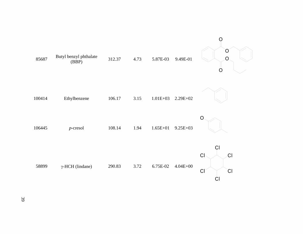
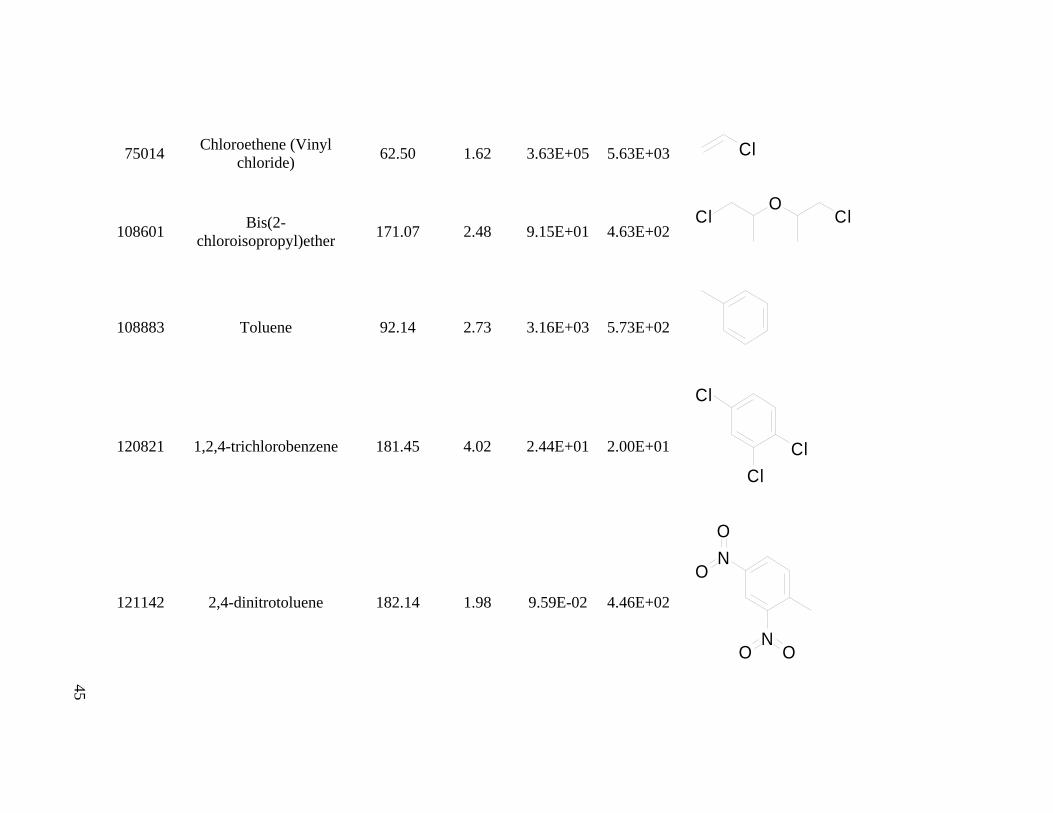
Table A-3. Summary of physical chemical properties and chemical structures for BIOWIN model calibrations.

CAS Name MW log Kow VP Sw Chemical Structure

(g/mol) (Pa) (mg/L)

71432 Benzene 78.11 2.13 1.16E+04 2.00E+03

84662 Diethylphthalate (DEP) 222.24 2.42 3.39E-01 2.87E+02

87865 Pentachlorophenol 266.34 5.12 1.44E-03 3.09E+00

O

O

O O

O

ClCl

ClCl

Cl

38

93765 2,4,5-

trichlorophenoxyacetic acid

255.49 3.31 9.36E-04 8.16E+01

108952 Phenol 94.11 1.46 4.31E+01 2.62E+04

1912249 Atrazine 215.69 2.61 3.81E-03 2.14E+02

O

OO

ClCl

Cl

O

N N

N N

N

Cl

39

85687 Butyl benzyl phthalate (BBP) 312.37 4.73 5.87E-03 9.49E-01

100414 Ethylbenzene 106.17 3.15 1.01E+03 2.29E+02

106445 p-cresol 108.14 1.94 1.65E+01 9.25E+03

58899 γ-HCH (lindane) 290.83 3.72 6.75E-02 4.04E+00

O

O

O

O

O

ClCl

ClCl

Cl

Cl

40

63252 Carbaryl 201.23 2.36 7.11E-03 4.16E+02

76448 Heptachlor 373.32 5.47 3.17E-02 2.76E-02

91203 Naphthalene 128.18 3.30 5.39E+00 1.42E+02

O

ON

Cl

Cl Cl

ClClCl

Cl

41

91225 Quinoline 129.16 2.03 7.19E+00 1.71E+03

95954 2,4,5-trichlorophenol 197.45 3.72 6.76E-01 1.14E+02

116063 Aldicarb 190.26 1.13 6.44E-01 5.31E+03

N

O

ClCl

Cl

O ON

SN

42

118741 Hexachlorobenzene 284.78 5.73 4.07E-04 1.92E-01

122349 Simazine 201.66 2.18 1.22E-03 5.90E+02

131113 Dimethylphthalate (DMP) 194.19 1.60 6.16E-01 2.01E+03

ClCl

ClCl

Cl

Cl

N N

N N

N

Cl

O

O

O O

43

1563662 Carbofuran 221.26 2.32 7.39E-03 3.54E+02

1746016 2,3,7,8-TCDD 321.98 6.80 2.60E-06 1.10E-03

1918009 Dicamba 221.04 2.21 7.05E-03 4.41E+02

O

OON

Cl O Cl

ClOCl

OCl

Cl

O

O

44

50328 Benzo[a]pyrene 252.32 6.13 2.65E-06 1.04E-02

56553 Benz[a]anthracene 228.30 5.76 3.63E-05 2.91E-02

72435 Methoxychlor 345.66 5.08 5.56E-03 3.02E-01

O O

ClCl Cl

45

75014 Chloroethene (Vinyl chloride) 62.50 1.62 3.63E+05 5.63E+03

108601 Bis(2-chloroisopropyl)ether 171.07 2.48 9.15E+01 4.63E+02

108883 Toluene 92.14 2.73 3.16E+03 5.73E+02

120821 1,2,4-trichlorobenzene 181.45 4.02 2.44E+01 2.00E+01

121142 2,4-dinitrotoluene 182.14 1.98 9.59E-02 4.46E+02

Cl

OCl Cl

ClCl

Cl

ONO

NO O

46

206440 Fluoranthene 202.26 5.16 4.17E-04 1.30E-01

7085190 Mecoprop 214.65 3.13 6.08E-02 1.94E+02

64175 Ethanol 46.07 -0.31 8.12E+03 7.92E+05

65850 Benzoic acid 122.12 1.87 3.97E-01 2.49E+03

O

OO

Cl

O

O

O

47

91941 3,3'-dichlorobenzidine 253.13 3.51 5.55E-04 2.29E+01

98862 Acetophenone 120.15 1.58 4.35E+01 4.48E+03

106423 p-xylene (Benzene, 1,4-dimethyl-) 106.17 3.15 9.16E+02 2.29E+02

107211 Ethylene glycol 62.07 -1.36 1.23E+01 1.00E+06

N

NCl

Cl

O

OO

48

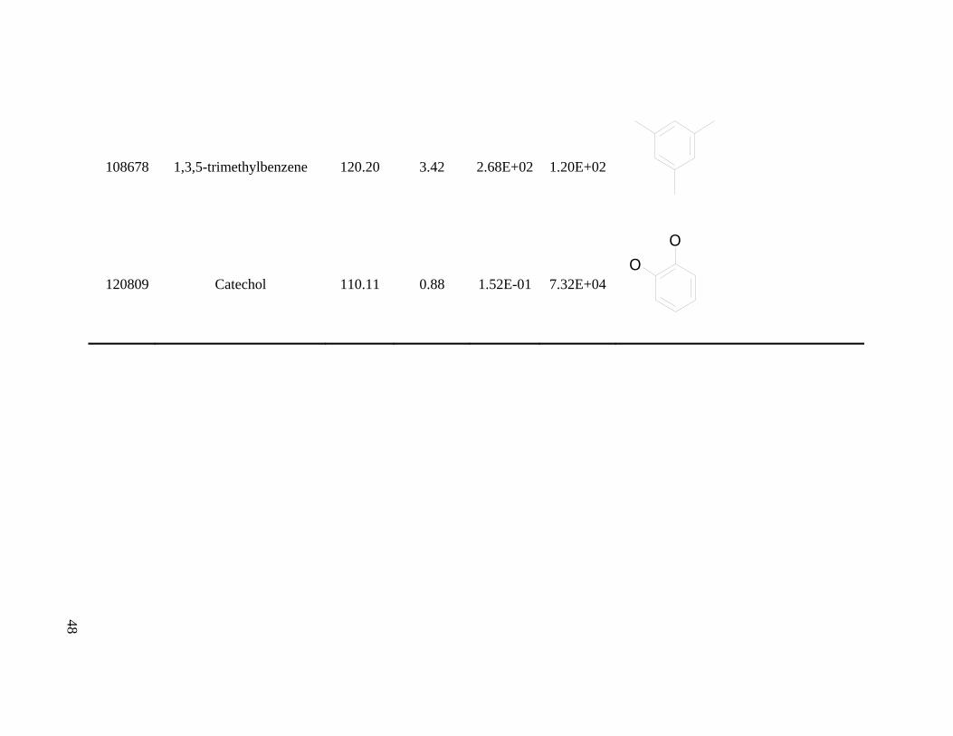
108678 1,3,5-trimethylbenzene 120.20 3.42 2.68E+02 1.20E+02

120809 Catechol 110.11 0.88 1.52E-01 7.32E+04

OO

development and application of models of chemical · pdf filedevelopment and application of...

Documents