developing rainfall intensityâ€“durationâ€“frequency...

Journal of King Saud University – Engineering Sciences (2012) 24, 131–140

King Saud University

Journal of King Saud University – Engineering Sciences

www.ksu.edu.sawww.sciencedirect.com

ORIGINAL ARTICLE

Developing rainfall intensity–duration–frequency

relationship for two regions in Saudi Arabia

Ibrahim H. Elsebaie *

Civil Engineering Department, King Saud University, College of Engineer, P.O. Box 800, Riyadh 11421, Riyadh, Saudi Arabia

Received 9 November 2010; accepted 21 June 2011

Available online 10 September 2011

*

E

10

El

Pe

do

KEYWORDS

IDF curve;

Rainfall intensity;

Rainfall duration;

Rainfall frequency

relationships

Corresponding author. Fax

-mail address: elsebaie@ksu

18-3639 ª 2011 King Saud

sevier B.V. All rights reserve

er review under responsibilit

i:10.1016/j.jksues.2011.06.00

Production and h

: +499 4

.edu.sa

Universit

d.

y of King

1

osting by E

Abstract Intensity–duration–frequency (IDF) relationship of rainfall amounts is one of the most

commonly used tools in water resources engineering for planning, design and operation of water

resources projects. The objective of this research is to derive IDF relationship of rainfall at Najran

and Hafr Albatin regions in the kingdom of Saudi Arabia (KSA). These relationships are useful in

the design of urban drainage works, e.g. storm sewers, culverts and other hydraulic structures. Two

common frequency analysis techniques were used to develop the IDF relationship from rainfall data

of these regions. These techniques are: Gumbel and the Log Pearson Type III distribution (LPT

III).

An equation for estimating rainfall intensity for each region was derived using both techniques.

The results obtained using Gumbel distribution are slightly higher than the results obtained using

the LPT III distribution. Rainfall intensities obtained from these two methods showed good agree-

ment with results from previous studies on some parts of the study area. The chi-square goodness-

of-fit test was used to determine the best fit probability distribution. The parameters of the IDF

equations and coefficient of correlation for different return periods (2, 5, 10, 25, 50 and 100) are

calculated by using non-linear multiple regression method. The results obtained showed that in

all the cases the correlation coefficient is very high indicating the goodness of fit of the formulae

to estimate IDF curves in the region of interest.ª 2011 King Saud University. Production and hosting by Elsevier B.V. All rights reserved.

677008.

y. Production and hosting by

Saud University.

lsevier

1. Introduction

Rainfall intensity–duration–frequency IDF curves are graphi-cal representations of the amount of water that falls within agiven period of time in catchment areas (Dupont and Allen,

2000). IDF curves are used to aid the engineers while designingurban drainage works. The establishment of such relationshipswas done as early as 1932 (see Chow (1988) and Dupont and

Allen (2006)). Since then, many sets of relationships have beenconstructed for several parts of the globe. However, such rela-tionships have not been accurately constructed in many devel-

oping countries (Koutsoyiannis et al., 1998).

mailto:[email protected]

http://dx.doi.org/10.1016/j.jksues.2011.06.001



http://www.sciencedirect.com/science/journal/10183639

Nomenclature

C the skewness coefficient;

I rainfall intensity;IDF Intensity–duration–frequency relationship;K Gumbel frequency factorKt Log Pearson frequency factor

n number of events or years of record;P* the logarithm of the extreme value of rainfall;Pave average of maximum precipitation corresponding

to a specific duration

Pi the individual extreme value of rainfall

PT the desired rainfall peak value for a specific fre-quency;

S standard deviation of P data;S* standard deviation of P* data;

T return period;Td rainfall duration;

132 I.H. Elsebaie

(Koutsoyiannis et al., 1998; Koutsoyiannis, 2003) cited thatthe IDF relationship is a mathematical relationship between therainfall intensity i, the duration d, and the return period T (or,equivalently, the annual frequency of exceedance f typically re-

ferred to as ‘frequency’ only). Indeed the IDF-curves allow forthe estimation of the return period of an observed rainfall eventor conversely of the rainfall amount corresponding to a given

return period for different aggregation times.In Kentucky, for example IDF curves are used in conjunc-

tion with runoff estimation formulae; e.g. the RationalMethod,

to predict the peak runoff amounts from a particular watershed.The information from the curves is then used in hydraulic designto size culverts and pipes (Dupont and Allen, 2000). Furtherstudies by Ilona and Frances (2002) performed rainfall analysis

and regionalisation of IDF curves for different regions.In recent studies, various authors attempted to relate IDF-

relationship to the synoptic meteorological conditions in the

area of the hydrometric stations (see Dupont and Allen(2006); Mohymont1 et al. (2004)). Al-Shaikh (1985) derivedrainfall depth–duration–frequency relationships (DDF) for

Saudi Arabia through the analysis of available rainfall inten-sity data. He added that Saudi Arabia could be divided intosix rainfall zones. These zones are: I South-western region, II

mountainous area along the Coast of the Red Sea, III North-ern region, IV Central and Eastern region, V Southern regionand VI Rob’a Al-Khaly region. Al-Shaikh, (1985) recom-mended that rainfall estimates from individual stations and re-

gional analysis may be modified in future when new rainfalldata become available.

Al-Dokhayel (1986) performed a study to estimate the rain-

fall depth duration frequency relationships for Qasim region inKSA at various return periods, using two continuous probabil-ity distributions, the extreme value type I distribution

(Gumbel) and the LPT III distribution. Al-Dokhayel (1986)found that among the two distributions used in the study,the LPT III distribution method gave some larger rainfall esti-mates with small standard errors. Al-Khalaf (1997) conducted

a study for predicting short-duration, high-intensity rainfall inSaudi Arabia. He found in the results that the short duration/high intensity rainfall was far from the universal relationship

suggested by other researchers and concluded that a relationfor each region has to be obtained to act as a useful tool inestimating rainfall intensities for different durations and return

periods ranging between 2 and 100 years. Further studies byAl-Sobayel (1983) and Al-Salem (1985) performed RainfallFrequency Distribution and analysis for Riyadh, Shaqra and

Al-Zilfi areas in KSA.

With the recent technology of remote sensing and satellitedata, Awadallah et al. (2011) conducted a study for developingIDF curves in scarce data region using regional analysis andsatellite data. Awadallah et al. (2011) presented a methodology

to overcome the lack of ground stations rainfall by the jointuse of available ground data with TRMM satellite data todevelop IDF curves and he used a method to develop ratios

between 24-hr rainfall depth and shorter duration depths.AlHassoun (2011) developed an empirical formula to

estimate the rainfall intensity in Riyadh region. He found that

there is not much difference in the results of rainfall analysis ofIDF curves in Riyadh area between Gumbel and LPT IIImethods. He attributed this to the fact that Riyadh regionhas semi-arid climate and flat topography where variations

of precipitation are not big.

2. Data collection

Data from different climatological stations in and aroundNajran city were obtained from the Ministry of Water and

Electricity, however, only one of these stations had a goodrecord (1967–2001) and time intervals (10, 20, 30, 60, 120,180 min, etc. . .) with few missing data and the other stations

have very few records of the data which are not presentableat all to be considered in the study. Also, data from seven rain-fall stations representing the Central and Eastern region were

available for different durations, but only Hafr AlBatin stationamong them had a good record (1967–2001) with the sametime intervals, as previously mentioned. These zones are shownin Fig. 1. The available rainfall data were analysed to deter-

mine the peak rainfall for each year.

3. Development of IDF curves

For accurate hydrologic analyses, reliable rainfall intensityestimates are necessary. The IDF relationship comprises the

estimates of rainfall intensities of different durations andrecurrence intervals. There are commonly used theoretical dis-tribution functions that were applied in different regions all

over the world; (e.g. Generalized Extreme Value Distribution(GEV), Gumbel, Pearson type III distributions) (see Dupontand Allen (2000); Nhat et al. (2006); Hadadin (2005);Acar and Senocak (2008); Oyebande (1982); Raiford et al.

(2007) and (AlHassoun, 2011). Two common frequencyanalysis techniques were used to develop the relationship be-tween rainfall intensity, storm duration, and return periods

from rainfall data for the regions under study. These

Figure 1 Rainfall zones in Saudi Arabia.

Developing rainfall intensity–duration–frequency relationship for two regions in Saudi Arabia 133

techniques are: Gumbel distribution and LPT III distribution.Either may be used as a formula or as a graphical approach.

3.1. Gumbel theory of distribution

Gumbel distribution methodology was selected to perform theflood probability analysis. The Gumbel theory of distributionis the most widely used distribution for IDF analysis owing toits suitability for modelling maxima. It is relatively simple and

uses only extreme events (maximum values or peak rainfalls).The Gumbel method calculates the 2, 5, 10, 25, 50 and 100-year return intervals for each duration period and requires sev-

eral calculations. Frequency precipitation PT (in mm) for eachduration with a specified return period T (in year) is given bythe following equation.

PT ¼ Pave þ KS ð1Þ

where K is Gumbel frequency factor given by:

K ¼ �ffiffiffi6p

p0:5772þ ln ln

T

T� 1

� �� ð2Þ

where Pave is the average of the maximum precipitation corre-

sponding to a specific duration.In utilising Gumbel’s distribution, the arithmetic average in

Eq. (1) is used:

Pave ¼1

n

Xni¼1

Pi ð3Þ

where Pi is the individual extreme value of rainfall and n isthe number of events or years of record. The standard devia-

tion is calculated by Eq. (4) computed using the followingrelation:

S ¼ 1

n� 1

Xni¼1ðPi � PaveÞ2

" #1=2ð4Þ

where S is the standard deviation of P data. The frequencyfactor (K), which is a function of the return period and sample

size, when multiplied by the standard deviation gives thedeparture of a desired return period rainfall from the average.Then the rainfall intensity, I (in mm/h) for return period T is

obtained from:

It ¼Pt

Td

ð5Þ

where Td is duration in hours.The frequency of the rainfall is usually defined by reference

to the annual maximum series, which consists of the largest

values observed in each year. An alternative data format forrainfall frequency studies is that based on the peak-over-threshold concept, which consists of all precipitation amounts

above certain thresholds selected for different durations. Dueto its simpler structure, the annual-maximum-series methodis more popular in practice (see Borga, Vezzani and Fontana,

2005).From the raw data, the maximum precipitation (P) and the

statistical variables (average and standard deviation) for eachduration (10, 20, 30, 60, 120, 180, 360, 720, 1440 min) were

computed. Tables 1 and 2 show the computed frequencyprecipitation (PT) values and intensities (IT) for different

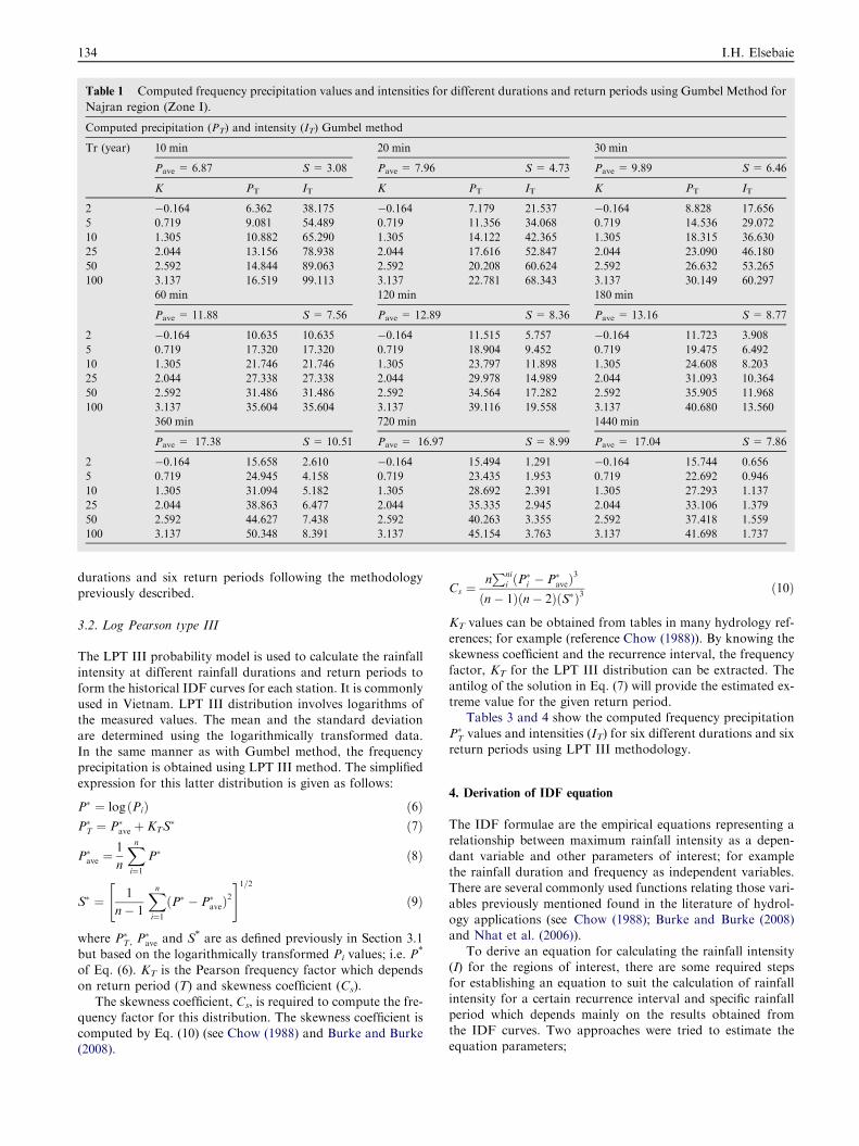
Table 1 Computed frequency precipitation values and intensities for different durations and return periods using Gumbel Method for

Najran region (Zone I).

Computed precipitation (PT) and intensity (IT) Gumbel method

Tr (year) 10 min 20 min 30 min

Pave = 6.87 S= 3.08 Pave = 7.96 S= 4.73 Pave = 9.89 S= 6.46

K PT IT K PT IT K PT IT

2 �0.164 6.362 38.175 �0.164 7.179 21.537 �0.164 8.828 17.656

5 0.719 9.081 54.489 0.719 11.356 34.068 0.719 14.536 29.072

10 1.305 10.882 65.290 1.305 14.122 42.365 1.305 18.315 36.630

25 2.044 13.156 78.938 2.044 17.616 52.847 2.044 23.090 46.180

50 2.592 14.844 89.063 2.592 20.208 60.624 2.592 26.632 53.265

100 3.137 16.519 99.113 3.137 22.781 68.343 3.137 30.149 60.297

60 min 120 min 180 min


2 �0.164 10.635 10.635 �0.164 11.515 5.757 �0.164 11.723 3.908

5 0.719 17.320 17.320 0.719 18.904 9.452 0.719 19.475 6.492

10 1.305 21.746 21.746 1.305 23.797 11.898 1.305 24.608 8.203

25 2.044 27.338 27.338 2.044 29.978 14.989 2.044 31.093 10.364

50 2.592 31.486 31.486 2.592 34.564 17.282 2.592 35.905 11.968

100 3.137 35.604 35.604 3.137 39.116 19.558 3.137 40.680 13.560

360 min 720 min 1440 min


2 �0.164 15.658 2.610 �0.164 15.494 1.291 �0.164 15.744 0.656

5 0.719 24.945 4.158 0.719 23.435 1.953 0.719 22.692 0.946

10 1.305 31.094 5.182 1.305 28.692 2.391 1.305 27.293 1.137

25 2.044 38.863 6.477 2.044 35.335 2.945 2.044 33.106 1.379

50 2.592 44.627 7.438 2.592 40.263 3.355 2.592 37.418 1.559

100 3.137 50.348 8.391 3.137 45.154 3.763 3.137 41.698 1.737

134 I.H. Elsebaie

durations and six return periods following the methodologypreviously described.

3.2. Log Pearson type III

The LPT III probability model is used to calculate the rainfallintensity at different rainfall durations and return periods to

form the historical IDF curves for each station. It is commonlyused in Vietnam. LPT III distribution involves logarithms ofthe measured values. The mean and the standard deviation

are determined using the logarithmically transformed data.In the same manner as with Gumbel method, the frequencyprecipitation is obtained using LPT III method. The simplified

expression for this latter distribution is given as follows:

P� ¼ log ðPiÞ ð6ÞP�T ¼ P�ave þ KTS

� ð7Þ

P�ave ¼1

n

Xni¼1

P� ð8Þ

S� ¼ 1

n� 1

Xni¼1ðP� � P�aveÞ

2

" #1=2ð9Þ

where P�T, P�ave and S* are as defined previously in Section 3.1

but based on the logarithmically transformed Pi values; i.e. P*

of Eq. (6). KT is the Pearson frequency factor which dependson return period (T) and skewness coefficient (Cs).

The skewness coefficient, Cs, is required to compute the fre-quency factor for this distribution. The skewness coefficient iscomputed by Eq. (10) (see Chow (1988) and Burke and Burke(2008).

Cs ¼nPni

i ðP�i � P�aveÞ3

ðn� 1Þðn� 2ÞðS�Þ3ð10Þ

KT values can be obtained from tables in many hydrology ref-

erences; for example (reference Chow (1988)). By knowing theskewness coefficient and the recurrence interval, the frequencyfactor, KT for the LPT III distribution can be extracted. The

antilog of the solution in Eq. (7) will provide the estimated ex-treme value for the given return period.

Tables 3 and 4 show the computed frequency precipitation

P�T values and intensities (IT) for six different durations and sixreturn periods using LPT III methodology.

4. Derivation of IDF equation

The IDF formulae are the empirical equations representing arelationship between maximum rainfall intensity as a depen-

dant variable and other parameters of interest; for examplethe rainfall duration and frequency as independent variables.There are several commonly used functions relating those vari-

ables previously mentioned found in the literature of hydrol-ogy applications (see Chow (1988); Burke and Burke (2008)and Nhat et al. (2006)).

To derive an equation for calculating the rainfall intensity(I) for the regions of interest, there are some required stepsfor establishing an equation to suit the calculation of rainfall

intensity for a certain recurrence interval and specific rainfallperiod which depends mainly on the results obtained fromthe IDF curves. Two approaches were tried to estimate theequation parameters;

Table 2 Computed frequency precipitation values and intensities for different durations and return periods using Gumbel Method for

Hafr AlBatin (Zone IV).

Computed precipitation (PT) and intensity (IT) Gumbel method

Tr (year) 10 min 20 min 30 min


K PT IT K PT IT K PT IT

2 �0.164 7.667 46.002 �0.164 9.689 29.068 �0.164 10.999 21.998

5 0.719 11.902 71.414 0.719 15.078 45.233 0.719 17.191 34.382

10 1.305 14.706 88.239 1.305 18.645 55.936 1.305 21.290 42.581

25 2.044 18.249 109.497 2.044 23.153 69.459 2.044 26.470 52.940

50 2.592 20.878 125.268 2.592 26.497 79.491 2.592 30.313 60.626

100 3.137 23.487 140.922 3.137 29.816 89.449 3.137 34.127 68.254

60 min 120 min 180 min


2 �0.164 13.391 13.391 �0.164 15.699 7.849 �0.164 17.866 5.955

5 0.719 20.757 20.757 0.719 24.425 12.213 0.719 26.453 8.818

10 1.305 25.635 25.635 1.305 30.203 15.101 1.305 32.138 10.713

25 2.044 31.797 31.797 2.044 37.502 18.751 2.044 39.321 13.107

50 2.592 36.368 36.368 2.592 42.918 21.459 2.592 44.650 14.883

100 3.137 40.906 40.906 3.137 48.293 24.147 3.137 49.940 16.647

360 min 720 min 1440 min


2 �0.164 19.190 3.198 �0.164 21.072 1.756 �0.164 28.754 1.198

5 0.719 28.235 4.706 0.719 30.764 2.564 0.719 42.297 1.762

10 1.305 34.224 5.704 1.305 37.182 3.099 1.305 51.263 2.136

25 2.044 41.791 6.965 2.044 45.291 3.774 2.044 62.593 2.608

50 2.592 47.405 7.901 2.592 51.306 4.276 2.592 70.997 2.958

100 3.137 52.977 8.829 3.137 57.277 4.773 3.137 79.340 3.306


A. By applying the logarithmic conversion, where it is pos-sible to convert the equation into a linear equation, and thus tocalculate all the parameters related to the equation. The fol-

lowing steps are followed to derive an1. Convert the original equation in the form of power-law

relation (see Chow (1988); Koutsoyiannis et al. (1998),and AlHassoun (2011)) as follows:

m

I ¼ CTr

Ted

ð11Þ

By applying the logarithmic function to get

log I ¼ log K� e log Td ð12Þ

where

K ¼ CTmr ð13Þ

and e represents the slope of the straight line

2. Calculate the natural logarithm for (K) value found from

Gumbel method or from LPT III method as well as thenatural logarithmic for rainfall period Td.

3. Plot the values of (log I) on the y -axis and the value of

(logTd) on the x axis for all the recurrence intervals forthe two methods.

4. From the graphs (or mathematically) we find the value of

(e) for all recurrence intervals where, then we find out theaverage e value, eave, by using the following equation:P
eave ¼
e

nð14Þ

where n represents recurrence intervals (years) valuenoted as Tr.

5. From the graph, we find (logK) values for each recur-

rence interval where (logK) represents the Y-intercept val-ues as per Gumbel method or LPT III method. Then weconvert Eq. (13) into a linear equation by applying thenatural logarithm to become:

log K ¼ log cþm log Tr ð15Þ

6. Plot the values of (logK) on the y-axis and the values of(logTr) on the x-axis to find out the values of parametersc and m as per Gumbel method or LPT III where (m) rep-

resents the slope of the straight line and (c) represents the(anti log) for the y intercept.

B. Estimation of the equation parameters by using non lin-ear regression analysis: Using the SOLVER function ofthe ubiquitous spreadsheet programme Microsoft Excel,which employs an iterative least squares fitting routine

to produce the optimal goodness of fit between dataand function. The R2 value calculated is designed to givethe user an estimate of goodness of fit of the function to

the data.

5. Goodness of fit test

The aim of the test is to decide how good is a fit between theobserved frequency of occurrence in a sample and the expected

Table 3 Computed frequency precipitation values and intensities for different durations and return periods using LPT III Method for

Najran region (Zone I).

Computed precipitation (PT) and intensity (IT) (Log Person III method)

Tr (year) Duration(min)

10 20 30

KT P�T PT IT KT P�T PT IT KT P�T PT IT

2 0.089 0.811 6.473 38.837 0.075 0.838 6.886 20.659 0.050 0.913 8.185 16.371

5 0.856 0.970 9.327 55.963 0.856 1.066 11.646 34.937 0.853 1.163 14.541 29.082

10 1.210 1.043 11.040 66.240 1.224 1.174 14.917 44.750 1.245 1.284 19.249 38.499

25 1.551 1.114 12.987 77.922 1.587 1.280 19.043 57.128 1.643 1.408 25.592 51.184

50 1.754 1.155 14.305 85.832 1.806 1.344 22.065 66.196 1.890 1.485 30.540 61.079

100 1.949 1.196 15.698 94.186 2.012 1.404 25.354 76.061 2.104 1.551 35.593 71.187

60 120 180

2 0.048 1.000 10.006 10.006 0.027 1.029 10.686 5.343 �0.042 1.032 10.769 3.590

5 0.853 1.236 17.230 17.230 0.848 1.268 18.515 9.258 0.827 1.256 18.041 6.014

10 1.246 1.352 22.478 22.478 1.263 1.388 24.429 12.215 1.305 1.380 23.965 7.988

25 1.647 1.469 29.459 29.459 1.694 1.513 32.605 16.302 1.834 1.516 32.805 10.935

50 1.896 1.542 34.851 34.851 1.967 1.592 39.126 19.563 2.185 1.607 40.423 13.474

100 2.111 1.606 40.323 40.323 2.208 1.662 45.958 22.979 2.508 1.690 48.974 16.325

360 720 1440

2 0.028 1.174 14.919 2.487 0.209 1.306 20.245 1.687 0.186 1.224 16.733 0.697

5 0.849 1.392 24.664 4.111 0.839 1.435 27.249 2.271 0.846 1.373 23.607 0.984

10 1.262 1.502 31.760 5.293 1.066 1.482 30.335 2.528 1.099 1.430 26.923 1.122

25 1.691 1.616 41.311 6.885 1.244 1.518 32.991 2.749 1.307 1.477 30.014 1.251

50 1.962 1.688 48.762 8.127 1.330 1.536 34.345 2.862 1.413 1.501 31.709 1.321

100 2.200 1.752 56.440 9.407 1.390 1.548 35.332 2.944 1.490 1.519 33.021 1.376

Table 4 Computed frequency precipitation values and intensities for different durations and return periods using LPT III Method for

Hafr AlBatin (Zone IV).

Computed precipitation (PT) and intensity (IT) (Log Person III method)

Tr (year) Duration (min)

10 20 30

KT P�T PT IT KT P�T PT IT KT P�T PT IT

2 0.104 0.895 7.844 47.062 0.066 0.975 9.448 28.344 0.000 1.019 10.448 20.896

5 0.857 1.095 12.454 74.722 0.855 1.182 15.210 45.630 0.845 1.224 16.765 33.531

10 1.200 1.187 15.373 92.239 1.231 1.281 19.084 57.251 1.260 1.325 21.149 42.297

25 1.500 1.267 18.483 110.896 1.606 1.379 23.930 71.790 1.715 1.436 27.282 54.563

50 1.700 1.320 20.898 125.386 1.834 1.439 27.460 82.379 1.999 1.505 31.981 63.962

100 1.850 1.360 22.914 137.483 2.029 1.490 30.889 92.667 2.251 1.566 36.825 73.650

60 120 180

2 �0.030 1.103 12.683 12.683 0.066 1.192 15.548 7.774 �0.042 1.239 17.352 5.784

5 0.831 1.299 19.892 19.892 0.855 1.379 23.938 11.969 0.827 1.403 25.294 8.431

10 1.299 1.405 25.406 25.406 1.231 1.468 29.403 14.701 1.313 1.495 31.232 10.411

25 1.811 1.521 33.202 33.202 1.606 1.557 36.096 18.048 1.865 1.599 39.684 13.228

50 2.149 1.598 39.619 39.619 1.834 1.612 40.889 20.445 2.236 1.669 46.616 15.539

100 2.458 1.668 46.564 46.564 2.029 1.658 45.491 22.745 2.580 1.733 54.120 18.040

360 720 1440

2 �0.138 1.258 18.134 3.022 �0.064 1.311 20.476 1.706 �0.075 1.441 27.637 1.152

5 0.775 1.416 26.073 4.346 0.817 1.466 29.269 2.439 0.812 1.603 40.132 1.672

10 1.338 1.513 32.617 5.436 1.316 1.554 35.833 2.986 1.320 1.696 49.696 2.071

25 2.003 1.628 42.493 7.082 1.877 1.653 44.986 3.749 1.900 1.802 63.433 2.643

50 2.471 1.709 51.187 8.531 2.256 1.720 52.459 4.372 2.300 1.875 75.060 3.127

100 2.917 1.786 61.122 10.187 2.608 1.782 60.507 5.042 2.650 1.939 86.969 3.624

136 I.H. Elsebaie

frequencies obtained from the hypothesised distributions. Agoodness-of-fit test between observed and expected frequen-

cies is based on the chi-square quantity, which is expressedas,

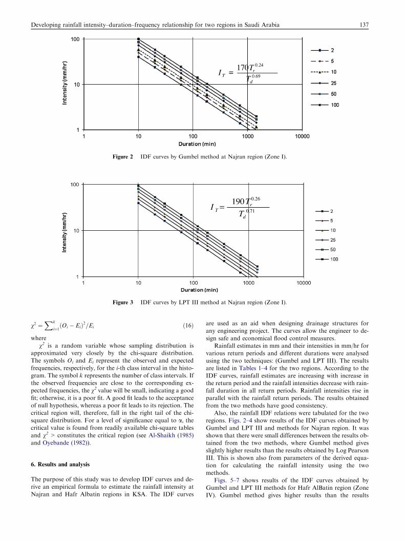
Figure 2 IDF curves by Gumbel method at Najran region (Zone I).

Figure 3 IDF curves by LPT III method at Najran region (Zone I).


v2 ¼Xk

i¼1ðOi � EiÞ2=Ei ð16Þ

wherev2 is a random variable whose sampling distribution is

approximated very closely by the chi-square distribution.The symbols Oi and Ei represent the observed and expected

frequencies, respectively, for the i-th class interval in the histo-gram. The symbol k represents the number of class intervals. Ifthe observed frequencies are close to the corresponding ex-

pected frequencies, the v2 value will be small, indicating a goodfit; otherwise, it is a poor fit. A good fit leads to the acceptanceof null hypothesis, whereas a poor fit leads to its rejection. The

critical region will, therefore, fall in the right tail of the chi-square distribution. For a level of significance equal to a, thecritical value is found from readily available chi-square tables

and v2 > constitutes the critical region (see Al-Shaikh (1985)and Oyebande (1982)).

6. Results and analysis

The purpose of this study was to develop IDF curves and de-rive an empirical formula to estimate the rainfall intensity at

Najran and Hafr Albatin regions in KSA. The IDF curves

are used as an aid when designing drainage structures for

any engineering project. The curves allow the engineer to de-sign safe and economical flood control measures.

Rainfall estimates in mm and their intensities in mm/hr for

various return periods and different durations were analysedusing the two techniques: (Gumbel and LPT III). The resultsare listed in Tables 1–4 for the two regions. According to the

IDF curves, rainfall estimates are increasing with increase inthe return period and the rainfall intensities decrease with rain-fall duration in all return periods. Rainfall intensities rise inparallel with the rainfall return periods. The results obtained

from the two methods have good consistency.Also, the rainfall IDF relations were tabulated for the two

regions. Figs. 2–4 show results of the IDF curves obtained by

Gumbel and LPT III and methods for Najran region. It wasshown that there were small differences between the results ob-tained from the two methods, where Gumbel method gives

slightly higher results than the results obtained by Log PearsonIII. This is shown also from parameters of the derived equa-tion for calculating the rainfall intensity using the two

methods.Figs. 5–7 shows results of the IDF curves obtained by

Gumbel and LPT III methods for Hafr AlBatin region (ZoneIV). Gumbel method gives higher results than the results

Figure 4 IDF curves by average at Najran region (Zone I).

Figure 5 IDF curves by Gumbel method at Hafr AlBatin (Zone IV).

Figure 6 IDF curves by LPT III method at Hafr AlBatin (Zone IV).

138 I.H. Elsebaie

Figure 7 IDF curves by average at Hafr AlBatin (Zone IV).

Table 5 The parameters values used in deriving formulas.

Region Parameter Gumbel Log Pearson III

Najran (Zone I) c 170 190

m 0.24 0.26

e 0.69 0.71

Hafr AlBatin

(Zone IV)

c 209 224

m 0.30 0.25

e 0.70 0.70

N.B: The parameters estimation of the IDF equations based on the

rainfall (mm), Rainfall intensities (mm/h) for different return per-

iod (years).


obtained by LPT III when they are applied to Zone IV. Alsothe trend of the results is the same and they are close to eachother.

Parameters of the selected IDF formula were adjusted by

the method of minimum squares, where the goodness of fit isjudged by the correlation coefficient. The results obtainedshowed that in all the cases the correlation coefficient is very

high, and ranges between 0.998 and 0.994, except few caseswhere it ranges between 0.983 and 0.978 when using LPT IIIat 50 and 100 years. This indicates the goodness of fit of the

formulae to estimate IDF curves in the region of interest.For each region the results are given as the mean value ofthe points results. Table 5 shows the parameters values ob-tained by analysing the IDF data using the two methods and

those are used in deriving formulae for the two regions.Also, goodness-of-fit tests were used to choose the best sta-

tistical distribution among those techniques. Results of the chi-

Table 6 Results of chi-square goodness of fit test on annual maxim

Region Distribution Duration in min

10 20

Najran Gumbel 0.575 0.175

Log Pearson type III 0.300 12.080

Central and Eastern region Gumbel 0.222 0.151

Log Pearson type III 2.081 3.420

For a = 0.05, degree of freedom= 1, the critical region is vcal > 3.84.

For a = 0.01, degree of freedom= 1, the critical region is vcal > 6.63.* v2 Significant at a = 0.01.

square goodness of fit test on annual series of rainfall areshown in Table 6. As it is seen most of the data fit the distri-

butions at the level of significance of a = 0.05, which yieldsvcal < 3.84. Only the data of Najran for 20 min and1440 min do not give good fit using the Log Pearson type IIIdistribution. Also, the data of Central and Eastern region for

120 min and 720 min do not give good fit, even at the levelof significance of a = 0.01.

7. Conclusions

This research presents some insight into the way in which the

rainfall is estimated in KSA. Since the area of the Kingdom islarge and has different climatic conditions from region to re-gion, a relation for each region has to be obtained to estimate

rainfall intensities for different durations and return periodsranging between 2 and 100 years.

This study has been conducted for the formulation and con-

struction of IDF curves using data from recording stations byusing two distribution methods: Gumbel and LPT III distribu-tion. Gumbel method gave some larger rainfall intensity esti-mates compared to LPT III distribution. In general, the

results obtained using the two approaches are very close atmost of the return periods and have the same trend, this agreeswith the results obtained by Al-Shaikh (1985) and AlHassoun

(2011). The results obtained from that work are consistent withthe results from previous studies done in some parts of thestudy area. It is concluded that the difference observed be-

tween the results of this study and the results done before byAl-Shaikh (1985) are accepted and in good agreement, and this

um rainfall.

utes

30 60 120 180 360 720 1440

0.360 0.373 0.489 0.929 0.190 0.228 0.260

4.667 5.161 0.522 0.540 0.242 1.438 7.620*

0.431 0.535 0.379 0.562 0.774 0.552 0.446

0.566 2.310 12.041* 1.751 6.861 8.048* 1.296

140 I.H. Elsebaie

can be attributed to the record lengths of the rainfall data used

for this study and the studies before.The parameters of the design storm intensity for a given

period of recurrence were estimated for each region. The re-sults obtained showed a good match between the rainfall inten-

sity computed by the methods used and the values estimatedby the calibrated formulae. The results showed that in all thecases data fitted the formula with a correlation coefficient

greater than 0.978. This indicates the goodness of fit of the for-mulae to estimate IDF curves in the region of interest for dura-tions varying from 10 to 1440 min and return periods from 2 to

100 years.The chi-square test was used on one hand to examine the

combinations or contingency of the observed and theoretical

frequencies, and on the other hand, to decide about the typeof distribution which the available data set follows. The resultsof the chi-square test of goodness of fit showed that in all thedurations the null hypothesis that the extreme rainfall series

have the Gumbel distribution is acceptable at the 5% level ofsignificance, this agrees with the results obtained by Oyebande(1982). Only few cases in which the fitting was not good

(20 min, 120 min and 720 min) obtained by using the LPT IIIdistribution. Although the chi-square values are appreciably be-low the critical region usingGumbel distribution and few values

are higher than the critical region using LPT III distribution, it isdifficult to say that one distribution is superior to the other. Fur-ther studies are recommended whenever there will be more datato verify the results obtained or update the IDF curves.

Acknowledgements

The writer expresses his sincere gratitude to the Research Cen-ter of the Faculty of Engineering, King Saud University, for

supporting this work. The writer is thankful to the Ministryof Water and Electricity, KSA for providing the data neededfor the research.

References

Acar, Resat and Senocak, Serkan. 2008. Modelling of Short Duration

Rainfall Intensity Equations for Ankara, Turkey, BALWOIS 2008-

Ohrid, Republic of Macedonia-27.

Al-Dokhayel, A.A. 1986. Regional rainfall frequency analysis for

Qasim, B.S. Project, Civil Engineering Department, King Saud

University, Riaydh (K.S.A), April, 1986.

AlHassoun, S.A., 2011. Developing an empirical formulae to estimate

rainfall intensity in Riyadh region. Journal of King Saud Univer-

sity-Engineering Sciences.

Al-Khalaf, H.A. 1997. Predicting short-duration, high-intensity rain-

fall in Saudi Arabia, M.S. Thesis, Faculty of the College of

Graduate Studies; King Fahad University of Petroleum and

Minerals, Dahran (K.S.A), 1997.

Al-Salem, H.S. 1985. Rainfall Frequency Distribution in Shaqra and

Al-Zilfi Areas, B.S. Project, Civil Engineering Department, King

Saud University, Riaydh, KSA, Jan. 1985.

Al-Shaikh, A.A. Rainfall frequency studies for Saudi Arabia, M.S.

Thesis, Civil Engineering Department, King Saud University,

Riaydh (K.S.A), 1985.

Al-Sobayel, A.E. 1983. Rainfall Frequency Distribution for Riyadh,

B.S. Project, Civil Engineering Department, King Saud University,

Riaydh (K.S.A), Jan. 1983.

Awadallah, A.G., ElGamal, M., ElMostafa, A., ElBadry, H., 2011.

Developing intensity–frequency curves in scarce data region: an

approach using regional analysis and satellite data. Scientific

Research Publishing, Engineering 3, 215–226.

Borga, M., Vezzani, C., Fontana, G.D. 2005. A Regional Rainfall

Depth–Duration–Frequency Equations for an Alpine Region,

Department of Land and AgroForest Environments, University

of Padova, Legnaro 35020, Italy, Natural Hazards, vol. 36, pp.

221–235.

Burke, C.B., Burke, T.T., 2008. Storm Drainage Manual. Indiana

LTAP.

Chow, V.T., 1988. Handbook of Applied Hydrology. McGraw-Hill

Book.

Dupont, B.S., Allen, D.L., 2000. Revision of the Rainfall Intensity

Duration Curves for the Commonwealth of Kentucky. Kentucky

Transportation Center, College of Engineering, University of

Kentucky, USA.

Dupont, B.S., Allen, D.L., 2006. Establishment of Intensity–Dura-

tion–Frequency Curves for Precipitation in the Monsoon Area of

Vietnam. Kentucky Transportation Center, College of Engineer,

University of Kentucky in corporation with US Department of

Transportation.

Hadadin, N.A., 2005. Rainfall intensity–duration–frequency relation-

ship in the Mujib basin in Jordan. Journal of Applied Science 8

(10), 1777–1784.

Ilona, V., Frances, F. 2002. Rainfall analysis and regionalization

computing intensity–duration–frequency curves, Universidad

Politecnica de Valencia – Departamento de Ingenieria Hidraulica

Medio Ambiente – APDO. 22012 – 46071 Valencia – Spain.

Koutsoyiannis, D. 2003. On the appropriateness of the Gumbel

distribution for modelling extreme rainfall, in: Proceedings of the

ESF LESC Exploratory Workshop, Hydrological Risk: recent

advances in peak river flow modelling, prediction and real-time

forecasting, Assessment of the impacts of land-use and climate

changes, European Science Foundation, National Research Coun-

cil of Italy, University of Bologna, Bologna, October 2003.

Koutsoyiannis, D., Kozonis, D., Manetas, A., 1998. A mathematical

framework for studying rainfall intensity–duration–frequency rela-

tionships. J. Hydrol. 206, 118–135.

Mohymont1, B., Demaree1, G.R., Faka2, D.N. 2004. Establishment

of IDF-curves for precipitation in the tropical area of Central

Africa – comparison of techniques and results, Department of

Meteorological Research and Development, Royal Meteorological

Institute of Belgium, Ringlaan 3, B-1180 Brussels, Belgium.

Nhat, L.M., Tachikawa, Y., Takara, K. 2006. Establishment of

intensity–duration–frequency Curves for Precipitation in the Mon-

soon Area of Vietnam’’, Annuals of Disas. Prev. Res. Inst., Kyoto

University, No. 49 B.

Oyebande, L., 1982. Deriving rainfall intensity–duration–frequency

relationships and estimates for regions with inadequate data.

Hydrological Science Journal 27 (3), 353–367.

Raiford, J.P., Aziz, N.M., Khan, A.A., Powel, D.N., 2007. Rainfall

depth–duration–frequency relationships for South Carolina, and

Georgia. American Journal of Environmental Sciences 3 (2), 78–84.

developing rainfall intensityâ€“durationâ€“frequency...

Documents