developing protection systems for microgrids by …
TRANSCRIPT

DEVELOPING PROTECTION SYSTEMS FOR MICROGRIDS
By
Mohamed Ali M. Mahmoud Esreraig
A THESIS
Submitted to
Michigan State University
in partial fulfillment of the requirements
for the degree of
MASTER OF SCIENCE
Electrical Engineering
2012

ABSTRACT
DEVELOPING PROTECTION SYSTEM FOR MICROGRIDS
By
Mohamed Ali M. Mahmoud Esreraig
Microgrid is an emerging form of power distribution system which is embedded with a
combination of different kinds of power generation sources, like renewable energy sources,
combined heat and power (CHP), and distributed energy resources (DER). The advantages of
Microgrid configuration are low transmission and distribution cost, and, potentially, high
reliability, high efficiency and low environmental impact.
Microgrids are designed to operate in one of two modes, grid connected and islanded. Short
circuit levels in islanded mode tend to be small compared to those in grid connected mode.
Moreover, power flows in microgrids are not always unidirectional. For these reasons, it is
difficult to protect microgrids using relaying strategies traditionally used in distribution systems.
In this research, a new approach is developed which uses a state observer as a fault detector to
identify faults that occur within the zone of protection. This system can be centralized or
decentralized, and needs only one current measurement and two end-voltage measurements for
each zone. An additional contribution of the research is a method of minimizing the required
number of measurements, subject to observability requirements. Using suitable voltage sensors,
and, where available, smart meters to measure voltages, it is possible to devise a low-cost
protection system using the proposed approach. The performance of the proposed method is
demonstrated on the IEEE 34 node test distribution feeder. The proposed approach is shown to
be effective in both grid-connected and islanded modes.

iii
TABLE OF CONTENTS
LIST OF TABLES .......................................................................................................................... v
LIST OF FIGURES ....................................................................................................................... vi
1. Introduction ............................................................................................................................. 1
2. Power Distribution Systems: Operations and Protection ........................................................ 5
2.1. Protection Considerations ................................................................................................ 5
2.1.1. Reliability:................................................................................................................. 5
2.1.2. Redundancy: ............................................................................................................. 7
2.1.3. Simplicity: ................................................................................................................. 7
2.1.4. Selectivity: ................................................................................................................ 7
2.1.5. Sensitivity: ................................................................................................................ 7
2.1.6. Speed of operation: ................................................................................................... 7
2.1.7. Consistency: .............................................................................................................. 7
2.2. Radial System ................................................................................................................... 8
2.2.1. Fault Analysis ........................................................................................................... 8
2.2.2. Protection Coordination ............................................................................................ 8
2.3. Ring System ................................................................................................................... 15
2.3.1. Contribution Currents ............................................................................................. 16
2.3.2. Protection Coordination .......................................................................................... 17
3. Protective Devices Coordination in DG Distribution System ............................................... 18
3.1. Fault Analysis ................................................................................................................. 18
3.2. Protection Coordination ................................................................................................. 18
4. Microgrids ............................................................................................................................. 25
4.1. Introduction .................................................................................................................... 25
4.2. Configuration of Microgrids .......................................................................................... 26
4.3. Control System in Microgrids ........................................................................................ 26
4.4. Protection issues in microgrids ...................................................................................... 28
5. Innovative Solutions for Protection Schemes in Microgrids ................................................. 30
5.1. Microgrid Protection Using Communication-Assisted Digital Relays .......................... 30
iv
5.2. Protecting Microgrid Systems containing Solid-State Converter Generation ............... 32
5.3. Integrated control and protection scheme for microgrid ................................................ 34
6. Microgrid Protection System Based on Observer and Minimum Measurements ................. 36
6.1. Introduction .................................................................................................................... 36
6.2. Microgrids Protection System Considerations ............................................................... 38
6.3. Theoretical Development of Observer-Based fault detector .......................................... 39
6.4. Application to Microgrid Protection .............................................................................. 44
6.4.1. Observer-Based fault detector behavior with different kinds of faults ................... 44
6.4.2. Minimum Measurements Placement....................................................................... 46
6.4.3. Protecting Transformers Using Observer ............................................................... 48
6.4.4. Multi-Zone Protection ............................................................................................. 49
6.5. Case Study ...................................................................................................................... 50
7. Discussion and Conclusion .................................................................................................... 62
REFERENCES ............................................................................................................................. 65

v
LIST OF TABLES
Table 2.1 Nominal currents for fuses used in the transformer high voltage side (10-12 KV) ...... 10
Table 2.2 The coordinated fuses nominal currents values (400 V and 10-12 KV) ...................... 10
Table 2.3 Overcurrent relay characteristics. ................................................................................. 12
Table 6.1 IEEE 34 node, transformer data .................................................................................... 59

vi
LIST OF FIGURES
Figure 2.1 Zones of protection ........................................................................................................ 6
Figure 2.2 Fuse to Fuse coordination in radial system. .................................................................. 8
Figure 2.3 Fuse to Fuse coordination using characteristic curve method. ...................................... 9
Figure 2.4 Radial system with short circuit currents on its busbars. ............................................ 13
Figure 2.5 Current time grading using standard inverse (SI) characteristic. ................................ 15
Figure 2.6 Ring system configuration, (a) one source ring system with directional relays, (b)
coordination of relays. .................................................................................................................. 16
Figure 3.1 Two ends DG's with directional Overcurrent relays. .................................................. 18
Figure 3.2 Current time grading for two ends generators. ............................................................ 19
Figure 3.3 Three DG's system with directional Overcurrent relays. ............................................ 20
Figure 3.4 Current time grading for Overcurrent Relays on three DG's system. ......................... 21
Figure 3.5 Four DG's system with directional Overcurrent relays. .............................................. 22
Figure 3.6 shows the three relays setting in the log scale. ............................................................ 23
Figure 4.1 Micogrid construction. ................................................................................................ 27
Figure 4.2 Schematic diagram of circuit breaker interconnection switch .................................... 28
Figure 5.1 Microgrid protection using communication-assisted digital relays. ............................ 31
Figure 5.2 Protecting microgrid systems containing solid-state converter generation. ................ 33
Figure 5.3 Schematics of pilot instantaneous overcurrent protection: (a) Overcurrent protection
coordination.(b) Pilot instantaneous protection for bus bar and feeder. ....................................... 35
Figure 6.1 A representation of one zone: (a) Single line diagram with in-zone loads, (b) Circuit
of one zone. ................................................................................................................................... 40
Figure 6.2 State observer as a fault detector. ................................................................................ 42
Figure 6.3 Equivalent network of single line to ground fault. ...................................................... 44

vii
Figure 6.4 Phase and earth fault observers connections of (a) Current transformers, (b) Voltage
transformers. ................................................................................................................................. 45
Figure 6.5 One phase of a power transformer with zero shift angle. ............................................ 48
Figure 6.6 Multi observer system (Bank of observers). ................................................................ 49
Figure 6.7 IEEE 34 node test feeder with protection zones. ......................................................... 52
Figure 6.8 Three phase fault (a) Line contribution currents, (b) phase residual gain correction (c)
phase observer residuals, and (d) phase to phase fault. ................................................................ 54
Figure 6.9 Single line to ground fault in zone K, (a) currents in zones K and H, (b) Phase
residuals of zones K and H, (c) Earth fault residuals of zones K and H. ...................................... 56
Figure 6.10 Phase and earth fault residuals of zone K in case of double phase to ground fault in
zone K. .......................................................................................................................................... 58
Figure 6.11 High resistance single line to ground fault in zone K. .............................................. 59
Figure 6.12 Observer’s behavior in case of: (a) steady state, (b) single line to ground fault at %50
of the primary winding of power transformer............................................................................... 60
Figure 7.1 A representation of backup zone (zone C). ................................................................. 63
1
1. Introduction
Electric power systems experience abnormal conditions like faults and disturbances which
lead to power interruptions, loss of stability and blackouts. To prevent or at least minimize the
fault consequences, a protection system is designed, installed and adjusted. Protection system
consists of different types of relays that have different characteristics and functions. Relays are
characterized according to their algorithms. Some are operated by high current values like
overcurrent relay, some by under and over voltage or frequency, and others by impedance like
distance relay. The requirement of redundancy is widespread in protection system. Hence, it is
common to protect equipment using more than one kind of relays. For example in transmission
lines the distance protection is the main and overcurrent is the backup protection. Redundancy is
applied to equipments in high and medium voltage networks but not to low voltage networks.
Communication channels are normally combined with protection systems of the high and
medium voltage networks. Power line carrier (PLC) and fiber optics communication systems are
common in power system networks. The modern protection systems use the telecommunications
for activating more functions in relays in the network. For instance, the line differential relay
uses communication channels (like fiber optics) to receive measurement information and send
trip signals to the remote end.
Deep understanding of basics and theories is very important to dealing with the distribution
system protection problems. Protection system is a complex system since it is affected by most
of changes and events in network, such as configuration changes, equipments outages, faults,
loading, and power system stability issues. As a result, protection engineers are following
different protection philosophies for designing and setting protection system. The cost of the
protection system depends on the network voltage levels: high, medium and low voltage levels.

2
High voltage equipments are more expensive than lower voltage levels and therefore their
protection system is more expensive. Nowadays, protective relays are using the digital
techniques which enable to include many functions in one relay. For high and medium voltage
level networks it is worthy, but for low voltage level networks it is expensive to use digital
relays.
Many kinds of protective relays have been developed according to their usage in the power
networks. There are two types of protection systems, unit protection and system protection. Unit
protection is to protect an equipment or zone but no need to set grading time with other
protective relays, an example of unit protection is the differential relay. System protection on the
other hand is consists of a time graded relays to protect a number of connected equipments;
Overcurrent and distance relays are examples of system protection. There are many types of
equipment protected by the two systems, like transformers and generators which are normally
protected by differential and overcurrent relays. Low voltage level network which is so called
distribution network is normally protected by fuses in downstream and overcurrent relays in
upstream.
The network configuration in the distribution system is mainly radial. However, because of
the new trend of operations, which depends on distributed generators DG's, the network
configuration changes. For traditional protection systems there are huge differences between
radial and DG networks. In the distribution Level, the protection system is overcurrent devices
(Fuse or Relay). This kind of protection is based on high current sensing.
In radial system, there is a graded difference between fault current values in downstream and
upstream. This difference makes it easy for overcurrent devices to be graded too. Overcurrent

3
relays have many different algorithms that can be mixed when protecting radial system. In
addition, all algorithms can be included in one relay which gives more flexibility to protection
engineers to design the proper protection system.
There are some differences between Fuses and relays. Fuses are less flexibility than relays and
care should be taken when dealing with fuses since their characteristics depend on melting
materials, so they should be from the same manufacturer. Moreover, fuses cannot be adjusted,
and then it should be selected carefully.
DG networks, on the other hand, are complex configuration that makes no rule for ordinary
protection system to be considered. In case of fault, every DG will contribute to the fault
depending on its size and characteristics. For example, power electronic devices maximum
contribution current value during fault is about twice their nominal current value.
The distribution of DG's over the network produces bidirectional currents which makes a very
important challenge for overcurrent devices. Although, there is a directional element can be
installed or activated in overcurrent relays, there will be some cases no longer this element
effective.
Moreover, DG sources are subject to be plugged in and out to the network at any time. This
makes considerable changes to the short circuit levels which needs different setting calculations.
Illustrating examples has been discussed for different kinds of networks; radial, ring and DG
networks.
In this research, configuration, control, and behavior of microgrids are discussed in details.
Microgrids are new developing philosophy in the power system networks. Operating microgrids
is complex since it should deal with many variables and changes in the microgrids and the utility.
4
The new power network is designed to overcome many power system impacts, such as
blackouts, cascading failures, lose of synchronism, and overloading, but controlling and
operating such a configuration is a challenge. Managing between small different kinds of DG’s
with the utility is not an easy task. DG’s are plug-and-play; configuration is changing according
to loading and disturbances in the utility or microgrids. Grid connected and islanded modes are
very different modes that make huge changes in short circuit levels [1] and [2].
Finally, this research discusses some literatures that propose solutions for microgrids
protection system. In addition, a novel protection system based on observer theory is presented.
This proposed protection system is built according voltage and current measurement data which
is carried out through the available microgrids communication system. The protection system
can be centralized or decentralized. If centralized, a multi observer system is constructed with
main control system of the microgrids and may be benefit from some measurements that are
already available for control and operation of microgrids. Decentralized protection system on the
other hand, can be mounted in protected zone itself; may be adapted with circuit breakers.
Observer-based protection system is simulated with different kinds of faults and in different
situations; load and contribution currents are examined as well. The simulation is performed
using Alternative Transient Program (ATP). To make the proposed protection system cost
effective, the number of measurement devices is reduced to the minimum but observable by the
protection system.

5
2. Power Distribution Systems: Operations and Protection
2.1.Protection Considerations
The protection system for any power system configuration, radial, ring, DG system or
microgrids must consider the requirements of designing and adjusting the protection
relays. These requirements are reliability, redundancy, simplicity, selectivity, sensitivity,
speed of operation, and consistency. Some of these requirements are designer’s
(manufacturer) responsibility, and others are protection engineers’ responsibility. Lack of
one of these requirements results in weakening the protection system. This research
focuses on most of these requirements in designing and adjusting the observer based
protection system. Its design is simple but reliable, selective, sensitive, and fast.
2.1.1. Reliability:
Reliability is a main factor that evaluates the protection system. There are two important
factors which make the protection system reliable or not. These are security and
dependability. Security is not to trip when it is not required to. The dependability on the
other hand is to trip when it is required to. The protection system is combined from many
types of relaying functions. Every relay in the protection system has its own zone to
protect from certain type of faults that relay is programmed against. Therefore, if any
relay missed operation for in-zone fault, the fault would extend to the next zone, and
therefore the next relay would operate. The problem here is that if one relay missed
operation the loss of load would be larger because the zone of protection extended which
result in isolating larger parts from the network. Dependability is easy to measure; any in-
zone fault that is not tripped by the protection is considered lack-of-dependability [3].

6
Figure 2.1 Zones of protection
The security of a protection system can be measured simply by comparing the number of
relay false trips related to external faults to the total number of external faults. This will
not be considering false trip that result from relay failure, power swings, inrush currents
or other phenomenon which are not classified as power system faults. The main purpose
of the relay, which is one component, is to function correctly to protect the system and
work as intended. Some other components may improve the reliability of power system
protection such as circuit breakers, measuring transformers, battery system, control
circuits, teleprotection devices, and any communication channels [3].
Practically, 100% dependability and 100% security cannot be obtained. 100%
dependability can be obtained by protecting the system when it trips as a result of any
fault which must be detectable. 100% security can be obtained by disabling the protection
system entirely but could not be tripped by it. High dependability and high security are
needed, but it is impossible to achieve both of them together. Generally, increasing one of

7
them will decrease the other, and vice versa. However, dependability and security may
not be penalized on their degree. The optimum combination between dependability and
security is the main purpose of a protection system design when they provide a suitable
reliability of the protection system [3].
2.1.2. Redundancy:
Redundancy is to add protective devices that have the same or different characteristics to
protect the same equipment. For example, the power transformer may be protected with
differential and overcurrent, so if one fails the other can protect the transformer.
2.1.3. Simplicity:
It is different to redundancy; it is minimum protective devices that could protect
equipment.
2.1.4. Selectivity:
It is the ability of the protective relays to distinguish between in zone and out-zone faults.
2.1.5. Sensitivity:
It is the ability of relay to respond to faults which appear in the protected zone.
2.1.6. Speed of operation:
It is fast isolation of faults to maintain equipment equipments from damage.
2.1.7. Consistency:
It is the ability of relay to restore its electrical and time properties.

8
2.2. Radial System
2.2.1. Fault Analysis
Fault current in radial configuration flows in one direction, from source to the fault, for all
fault types. For setting the protective relays, the radial configuration is the easiest since there is
no need for directional element and no in-feed effect.
2.2.2. Protection Coordination
Fuse to Fuse Coordination:
There are many standards for classifying fuses by the rated voltages, rated current,
time/current characteristics, and manufacturing characteristics [4]. To coordinate two or more
fuses in radial system as in figure 2.2, clearing energy ( 2. cI t ) for fuse 2 which is connected to
the load feeder should be less than the melting energy ( 2. mI t ) for the fuse 1.
Fuse 1
Fault
Fuse 2
tm
tm
I
I
t
t
Figure 2.2 Fuse to Fuse coordination in radial system.

9
There are three ways to coordinate fuses:
1- Selectivity ratio tables which are supplied by manufacturer. This is the ratio of nominal
currents for fuse 1 and fuse 2. The range of this ratio is from 1:3 to 1:1.25 and this ratio is
used in case of fuses from the same manufacturer.
Fuse 1
Fault
Fuse 2
Fuse 2 Fuse 1
Melting curve
clearing curve
I
t
Figure 2.3 Fuse to Fuse coordination using characteristic curve method.
2- Using characteristic curves (melting curves) which describe the relation between the
current and melting time and between current and total clearing time. This can be
performed by drawing fuses curves on one page, thus the fuse 1 melting curve should be
completely above that for fuse 2 clearing curve, Figure 2.3.
3- Using manufacturer selectivity tables. For example, Tables 2.1 and 2.2 are Siemens
company selectivity tables that used for protecting transformers. The first column shows
the transformer characteristic, while the second column shows the minimum value of fuse
nominal current ( minNI ) and that is for Magnetizing Inrush Current. In the third column,

10
the maximum fuse nominal current ( maxNI ) which is for reliable short circuit clearing, is
shown. Thus, selection a fuse with value should be between maximum and minimum
nominal current.
Table 2.1 Nominal currents for fuses used in the transformer high voltage side (10-12 KV)
Transformer Capacity KVA minNI Amps maxNI Amps
50 16 16
100 25 40
200 40 63
250 25 63
400 63 100
500 63 100
630 63 160
800 100 200
1000 100 200
Table 2.2 The coordinated fuses nominal currents values (400 V and 10-12 KV)
Low voltage Fuse capacity (Amps) High voltage Fuse capacity (Amps)
80 60
125 25
160 25
200 40
250 63
400 100
500 100
600 160
800 160
1000 200
11
Relay to Relay Coordination (Overcurrent Relay):
System protective relays must be coordinated to fulfill the selectivity requirement. In high and
medium voltage level networks there would be coordination between different kinds of relays. In
low voltage level distribution system, coordination is performed between overcurrent relays and
between relays and fuses. Overcurrent relays are magnitude and time relays. Hence, they pick up
for current values larger than their setting value and release trip signal according to their time
setting. Current and time settings are specified by protection engineers after running short circuit
programs to calculate the reasonable setting for each relay.
There are different algorithms that can process the currents input to the overcurrent relay
depending on the purpose of use. Normally overcurrent relays are functioning with all
characteristics. The simple characteristic is the definite time characteristic which its time
constant for the adjusted value of current and time does not change even if the current is multiple
of setting value. For example if the pickup current value is set to 1000 A and the time 0.3
seconds, the relay would work at 0.3 seconds when the fault current reaches 1000A or more.
Even if the current reaches 10000A, the relay would pick up at 0.3 seconds.
On the other hand, the inverse time characteristic operates according to the equations shown
in the Table 2.3 [5]. This characteristic is more flexible and then commonly used in power
distribution systems. The time of operation is inversely proportional to the fault current level and
the actual characteristic is a function of both: time and current settings. Inverse time
characteristic is number of curves which are arranged according to the time multiplier setting
(TMS), for example TMS=0.1 results in different operating time to that of 0.2 of the same
current value. The x axis of the plane represents the ratio of fault to setting current (current
setting multiplier).

12
Table 2.3 Overcurrent relay characteristics.
(a) Relay Characteristics to IEC 60255 Equation
Standard Inverse (SI) 0.02
0.14
1r
t TMSI
= ×−
Very Inverse (VI) 13.5
1r
t TMSI
= ×−
Extremely Inverse (EI) 2
80
1r
t TMSI
= ×−
Long Time Standard Earth Fault 120
1r
t TMSI
= ×−
(b) North American IDMT
Relay Characteristics Equation
IEEE Moderately Inverse 0.02
0.05150.114
7 1r
TDt
I
= × + −
IEEE Very Inverse 2
19.610.491
7 1r
TDt
I
= × + −
Extremely Inverse (EI) 2
28.20.1217
7 1r
TDt
I
= × + −
US CO8 Inverse 2
5.950.18
7 1r
TDt
I
= × + −
US CO2 Short Time Inverse 0.02
0.023940.01694
7 1r
TDt
I
= × + −
rs
II
I
=
, where sI is relay setting current
TMS is Time Multiplier Setting
TD is Time Dial Setting

13
The variety of characteristics of IDMT relays gives the relay coordination more flexibility. In the
same network, relays could be coordinated with different characteristics. In numerical relays,
more characteristics may be provided, standard and user-defined.
Relay Time Grading Margin:
A time interval should be allowed between the operations of two adjacent relays to achieve a
required discrimination between them. Grading margin is taking in account the protection system
errors from relay to circuit breaker and normally is chosen between 0.4 to 0.5 seconds [3], [5]
and [6].
Figure 2.4 Radial system with short circuit currents on its busbars.
For the radial network configuration in Figure 2.4, the relay current setting ( sI ) and TMS for
standard inverse (SI) characteristic can be calculated as follows:
R1 setting:
I=1200 A, choose sI =75% of CT ratio 100/1, the required trip time is t=0.1 sec.
120016
75r
s
II
I= = =

14
0.02
0.140.1
16 1TMS= ×
− , thus 0.04TMS = , in numerical relays this value can be found, but for
static and electromechanical relays may not. Therefore, adjusting sI to a new value could solve
this issue if the relay is mechanical or static version.
R2 setting:
Common time margins between relays are 0.4 and 0.5 seconds since the circuit breaker delays by
approximately 0.25 seconds and the relay processing time is about 0.15 seconds. Then, adding
0.4 seconds of time margin to R1 trip time (0.1 sec), t=0.1+0.4= 0.5sec.
For sI =100% of CT ratio 200/1,
12006
200rI = = and
0.140.5
0.026 1TMS= ×
−, thus 0.13TMS =
R3 setting:
First, the actual tripping time of R2 should be calculated at fault current I=2000A,
0.02
0.140.13 0.386 sec.
10 1t = × =
−
For R3, sI =100% of CT ratio 200/1,
0.02
0.140.386 0.4
10 1TMS+ = ×
−, thus 0.26TMS =
R4 setting:
First, the actual tripping time of R3 should be calculated at fault current I=3500A,
0.02
0.140.26 0.617 sec.
17.5 1t = × =
−
For R4, sI =100% of CT ratio 300/1,
0.02
0.140.617 0.4
11.66 1TMS+ = ×
−, thus 0.36TMS =

15
Figure 2.5 Current time grading using standard inverse (SI) characteristic. For interpretation of
the reference to color in this and all other figures, the reader is referred to the electronic version
of this thesis.
Relay to fuse coordination:
In distribution systems fuses are normally used in downstream and by using the operating time of
the upper fuse, time margin can be calculated to coordinate relays with fuses.
2.3. Ring System
The Ring Main configuration is a commonly used within distribution networks. The main reason
for using this configuration is to keep feeding consumers loads in case of faults occurring on the
interconnecting feeders. The configuration can be supplied through one source or two sources. A
typical ring main with overcurrent protection relays is shown in Figure 2.6a [5].
100
101
10-2
10-1
100
101
Multiple of currents (I/Is)
Tim
e (se
conds)
R2
R1
R4
R3

16
(a)
(b)
Figure 2.6 Ring system configuration, (a) one source ring system with directional relays, (b)
coordination of relays.
2.3.1. Contribution Currents
Faults in ring configuration may be fed from different directions, thus there would be
contribution currents that come from these directions, and therefore bidirectional overcurrent

17
relays cannot be coordinated. Current may flow in either direction through the various relay
locations; hence directional overcurrent relays are necessary.
2.3.2. Protection Coordination
Directional overcurrent relays in the ring main circuit can be graded by opening the ring at the
supply point. Based on the directionality, relays are divided into two groups and each group
graded separately, Figure 2.6b. Grading is starting from downstream towards the supply point.
The arrows shown in Figure 2.6b indicate the current direction that operates the relay. If two or
more power sources are available to feed the ring main circuit, it will be difficult to coordinate
the overcurrent protection. For the ring with two sources, there are two ways to coordinate
overcurrent relays. One way is to open the ring at one source using the high set instantaneous
overcurrent so that the ring could be graded as a single source [5]. The second way is to protect
the section between the two sources using unit protection, like differential protection, to consider
this section as one supply bus so that the rest of the ring can be considered as a ring with one
source.

18
3. Protective Devices Coordination in DG Distribution System
3.1. Fault Analysis
Since DG distribution system has many sources of power and currents, there would be
different contribution current directions and then make it hard for relays coordination [7] and [8].
3.2.Protection Coordination
Distributed generators have impacts on the protective relays with their contribution currents in
case of faults [9]. Overcurrent relay is the commonly used protective relay in distribution
systems. For high DG penetration, it is impossible to coordinate Overcurrent relays without
losing the selectivity of the protection system. The following examples are analyzing the
problem carefully.
Figure 3.1 shows four bus system with two end generators and directional overcurrent relays.
There should be directional overcurrent relays in the opposite ends of R1, R2, and R3.
R1 R2 R3
692 A697 A2079 A
G1 G2
Figure 3.1 Two ends DG's with directional Overcurrent relays.
R3 setting:
I=692 A, choose sI =100% of CT ratio 200/1, the required trip time is t=0.2 sec.
0.02
0.140.1
692( ) 1200
TMS= ×−
, thus 0.0359TMS = .
R2 setting:

19
Adding 0.4 sec. margin to R3 trip time (0.2 sec), t=0.2+0.4= 0.6sec.
I =692 A, sI =100% of CT ratio 200/1,
0.02
0.140.6
692( ) 1200
TMS= ×−
, thus 0.1TMS =
R1 setting:
First, the actual tripping time of R2 should be calculated at fault current I=697A,
0.02
0.140.1 0.55 sec.
697( ) 1200
t = × =−
For R1, sI =100% of CT ratio 300/1,
0.02
0.140.55 0.4
697( ) 1300
TMS+ = ×−
, thus 0.115TMS =
Figure 3.2 Current time grading for two ends generators.
100
101
10-2
10-1
100
101
Multiple of Currents (I/Is)
Tim
e (Seconds)
R2
R3
Note: For R3 and R2 Multiple of Currents ismultiple of 200 A, while for R1 is multiple of 300A
R1

20
Figure 3.2 shows the three relays setting in the log scale, thus we conclude that there is no
selectivity problem in this type of configurations for DG's.
If another DG is added to the last configuration Figure 3.1, the short circuit level would change.
Therefore a new setting should be applied to the protective relays. Figure 3.3 shows the new
configuration with a new short circuit level.
Figure 3.3 Three DG's system with directional Overcurrent relays.
R3 setting:
R3 senses the summation of contribution currents from DG1 and DG3 which is equal to 1274 A,
choose sI =100% of CT ratio 200/1, the required trip time is t=0.2 sec.
0.02
0.140.2
1274( ) 1200
TMS= ×−
, thus 0.053TMS = .
R2 setting:
Adding 0.4 seconds margin to R3 trip time (0.2 sec), t=0.2+0.4= 0.6sec.
I =692 A, sI =100% of CT ratio 200/1,
0.02
0.140.6
680( ) 1200
TMS= ×−
, thus 0.1TMS =

21
R1 setting:
First, the actual tripping time of R2 should be calculated at fault current I=697A,
0.02
0.140.1 0.55 sec.
697( ) 1200
t = × =−
For R1, sI =100% of CT ratio 300/1,
0.02
0.140.55 0.4
697( ) 1300
TMS+ = ×−
, thus 0.115TMS =
Figure 3.4 shows the three relays setting in the log scale, thus we conclude that there is no
selectivity problem in this type of configurations for DG's.
Figure 3.4 Current time grading for Overcurrent Relays on three DG's system.
100
101
10-2
10-1
100
101
Multiple of Currents (I/Is)
Tim
e (Seconds)
Note: For R3 and R2 Multiple of Currents is multiple of200 A, while for R1 is multiple of 300A
R1
R2
R3
22
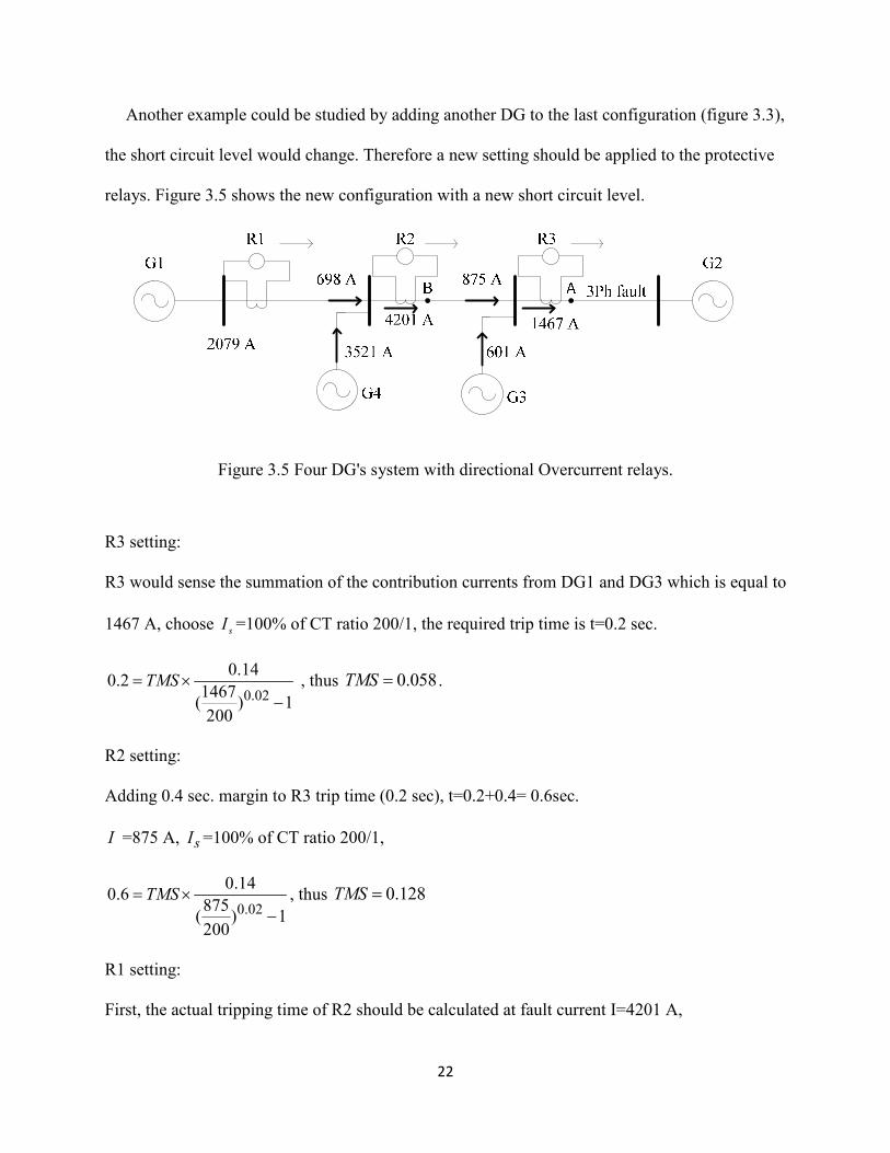
Another example could be studied by adding another DG to the last configuration (figure 3.3),
the short circuit level would change. Therefore a new setting should be applied to the protective
relays. Figure 3.5 shows the new configuration with a new short circuit level.
Figure 3.5 Four DG's system with directional Overcurrent relays.
R3 setting:
R3 would sense the summation of the contribution currents from DG1 and DG3 which is equal to
1467 A, choose sI =100% of CT ratio 200/1, the required trip time is t=0.2 sec.
0.02
0.140.2
1467( ) 1200
TMS= ×−
, thus 0.058TMS = .
R2 setting:
Adding 0.4 sec. margin to R3 trip time (0.2 sec), t=0.2+0.4= 0.6sec.
I =875 A, sI =100% of CT ratio 200/1,
0.02
0.140.6
875( ) 1200
TMS= ×−
, thus 0.128TMS =
R1 setting:
First, the actual tripping time of R2 should be calculated at fault current I=4201 A,

23
0.02
0.140.128 0.285 sec.
4201( ) 1200
t = × =−
For R1, sI =100% of CT ratio 300/1,
0.02
0.140.285 0.4
698( ) 1300
TMS+ = ×−
, thus 0.083TMS =
Figure 3.6 shows the three relays setting in the log scale.
Check selectivity:
For fault on A, R3 trips on 0.2 seconds, R2 trips on 0.6 seconds, and R1 trips on 0.685.
Therefore, we conclude that there is no coordination between R2 and R1 and they trips
simultaneously in case of fault at A.
We conclude that coordinating directional Overcurrent relays on high DG penetration
networks may not be valid for many network configurations. The effect of DG on coordination
100
101
10-1
100
101
Multiple of Current (I/Is)
Tim
e (Seconds)
R3
Note: For R3 and R2 Multiple of currents is multipleof 200 A, while for R1 is multiple of 300A
R2
R1

24
depends on size, type and placement of DG. In addition, DG based networks are characterized by
adding and isolating DG's according to loading or maintenance requirements. In this case, the
protection system setting needs to be recalculated according to the updated configuration.
Changing the setting in electromechanical and static relays is performed manually, which is
impractical.
Nowadays, numerical relays are commonly used and they have the ability to change from
setting group to another automatically. The setting calculation engineers perform setting groups
for all possible network configurations and upload these groups to relays either on site or
remotely. Numerical relays have inputs for this purpose (Binary Inputs), which can be connected
to the circuit breaker auxiliary contacts. Once the DG circuit breaker switches On or Off,
auxiliary contacts change their situation which triggers the relay binary inputs and make it to
change its setting to the required setting group. All numerical relays at a network can be
connected to the SCADA system which makes it easy to manage all of them to the required
setting [5].
The observer based protection system proposed in this research is adaptive with the network
changes and therefore does not need setting groups. It can detect the minimum and maximum in-
zone fault currents. It does not need grading time and that make it fast in clearing faults. In
addition, the proposed protection system is selective and does not respond to out-zone faults.
Therefore, the proposed system can protect DG power networks against faults and fulfilling
protection requirements.

25
4. Microgrids
4.1. Introduction
Microgrids are power system that combines numerous sources of power generation, like
renewable energy sources, combined heat and power (CHP), and distributed energy
resources (DER). This combination of different kind of generation is configured in a way to
guarantee continuing power supply to the load without interruption. Microgrids are designed
to lower cost, increase the efficiency, and help the environment. In other words, microgrids
are distribution system that would change the idea of being passive to be active networks by
distributing the decision making and control, in addition the power flows are bidirectional.
The output of the renewable energy sources is small and the environmental sources like
wind and sun are changing according to weather and season. Wind speed and sun shades can
control the output of renewable energy sources, and therefore storage is playing a main role
in the microgrids construction. Storage is also helping in reducing the cost of purchased
power especially in case of peak loads [10].
Using the modern controls and automatic operation technologies, the required reliability,
security, quality, and availability can be gained. In addition, making the sources near to the
load may improve the reliability.
The flexible configuration and operation of the microgrids helps in avoiding the
cascading failures. Thus, microgrids are designed to overcome issues like blackouts and lose
of stability. Microgrids can be attached to the utility (grid-connected) and isolated (islanded)
easily in case of faults in the utility.

26
4.2. Configuration of Microgrids
The idea of linking the power sources with consumer demands without interruptions
leads to a complex configuration. This kind of operation needs to connect the control system
using communication systems with information technologies. Distributed energy resources
like microturbines, fuel cells, photovoltaic (PV) arrays, wind farms together with storage
devices and controllable loads present control capabilities for the network operation.
Microgrids are formed as islands that have at least one distributed energy resource and
controllable loads. Sources and loads can be connected and disconnected to islands which
can do so to the medium voltage (MV) distribution system. Disconnecting microgrids from
the utility is called islanding mode. This mode result when the utility experience faults or
instability. Once the disturbance in the utility has cleared, microgrids could be connected
again. Figure 4.1 shows the construction of a microgrid that has numerous power sources
and controllable loads [11].
4.3. Control System in Microgrids
The fast development in information and communication technologies is promising for
low cost advanced monitoring and control of microgrids [12]. Control system of microgrids
should be designed to manage microgrids in grid-connected and islanded mode using
microgrid control center (MGCC), built in autonomous devices of DG’s, or both of them. In
grid connected mode the control system monitors and controls the voltage, power, and the
frequency for both, utility and microgrids, but in islanded mode, the control system monitors
and controls the microgrids. In addition, the control system may be designed to protect the
microgrids against faults and disturbances. Figure 4.2 shows the schematic diagram of a
circuit breaker based interconnection switch.

27
Figure 4.1 Micogrid construction.

28
DSP: Relay+ Comm +
Monitoring/Diagnostics
VT
CT
CT
VT
Circuit Breaker
DG
Load
Measurement
CommunicationUtility Grid
Figure 4.2 Schematic diagram of circuit breaker interconnection switch
Most of renewable energy sources are controlled using inverters control system which
makes these sources flexible for plug-and-play to the microgrid without any kind of
modification [13]. The idea of plug-and-play functionality can be described as using a home
appliance that can be plugged in and out to the electrical network at any location. Thus, the
same idea may be applied to DG’s to make generators near the heat loads, and therefore
efficient use of waste heat is guaranteed.
4.4. Protection issues in microgrids
Microgrids are designed to work in two modes, utility connected and stand-alone modes
(Islanded). When there are no disturbances in the utility network, Microgrids should be
connected to the utility grid. Otherwise, Microgrids work in islanded mode. This switching
between the two modes guarantees the power to be continued to the costumer without
interruptions, but it's difficult for the protection system to be effective in two modes.

29
One issue is that there would be small short circuit currents in islanded mode. Therefore,
the protection system could not detect the faults. Even if the fault is detected, another issue
would appear, that is the protection system could not be adjusted so that could work for both
modes. For instance, the overcurrent relays work in the current time characteristic, so the
trip time would be very large or infinity in case of islanded mode. Therefore, the ordinary
protection system could not overcome this issue.
Microgrids contain power electronic based DGs that behave differently to traditional
generators. DG's should be modeled differently in case of grid connected and islanded
mode. In grid connected mode should be modeled as constant power source, whereas
voltage with variable internal impedance in case of islanding.
This type of operation needs an adaptive protection system which can adapt to the
network changes, like switching between two modes and source outages. An idea of using
the numerical relays with the communication system could be useful, but the large cost was
a challenge.

30
5. Innovative Solutions for Protection Schemes in Microgrids
Much research has been reported on this issue and several solutions have been suggested. The
use of digital relays with the communication system in [14] offers an effective solution, but some
cases its cost may be unacceptably high. In [15] a d-q transformation method is used as fault
detection for microgrid system based on micro-sources equipped with power electronics
interfaces. Reference [16] proposes an integrated control and overcurrent protection interfacing
to the substation measurement devices and microgrid components through a substation optical
ethernet. References [17] and [18] propose that the protective functions should be part of the
distributed generator (DG).
5.1. Microgrid Protection Using Communication-Assisted Digital Relays
The development in protective relays presented the numerical relays as the most intelligent
relay. the relay contains inputs, outputs and microcomputer. The microcomputer uses predefined
and programmed or both algorithms to compare and calculate the input data. In addition,
numerical relays receives and sends signals from and to other relays and control centers. They
are programmable, using logic circuits, and have fiber optic and Ethernet communication links.
Moreover the relay has a memory to save events.
Reference [14] describes a new method to protect Microgrids using the ability of Numerical
relays to communicate with each other through the available communication medium.
Overcurrent relays have the ability to measure absolutely current sampled at 16 or higher number
of samples per cycle. Measured information can be transmitted through the communication
channels to the relay on the opposite side of the protected line segment. This technique is valid

31
for short lines, less than 18 miles, because the transmitted signal will take less than 0.1 ms based
on the light speed and around 0.15 ms for processing time. This technique is alternative to use
Phasor Measurement Units (PMU). For lines longer than 18 miles, using PMU may be required;
therefore, the differential relay is required. The basic concept of differential relay depends on the
two ends measurements and compares the difference to the threshold value. Differential relays
are instantaneous time relays.
In-1, In>
threshold?
Tx Common
Channel
Yes
Trip
Tx
TripPrimary
Device Fails
Backup
Device Fails
Communication
Channel Fails
Primary
Secondary
Tertiary
Alert relays that Differential
protection is lost
Alarm to distribution control
systemSwitch to comparative voltage
protection
RxRx
Figure 5.1 Microgrid protection using communication-assisted digital relays.

32
In case of circuit breaker failure tripping, a time delayed signal will be sent to the adjacent
relays on the same bus to force it to trip. If the relay or the communication media fails, all other
relays will be alerted that the differential schemes are lost. Relays will use the comparative
voltage protection which compares the relative rms voltage at each relay with the rest relays.
Figure 5.1 shows the described scheme.
To apply this method properly, many numerical relays are needed which will make the cost
very high.
5.2. Protecting Microgrid Systems containing Solid-State Converter Generation
The proposed protection scheme shown in figure 5.2 is based on converting measured abc
voltage values to dq values [15]. The detection algorithm converts abc voltages to a stationary dq
frame. Then, to convert to DC values the stationary frame is converted to a synchronous dq
frame.
This conversion can be performed using the following equations:
0
1 11
2 2
2 3 30
3 2 2
1 1 1
2 2 2
ds a
qs b
c
V v
V v
vV
− −
− =
cos sin2
sin cos3
dr ds
qr qs
V Vt t
V Vt t
ω ω
ω ω
− =

33
Therefore, any disturbance in the network will appear in the d-q values. To extract the
disturbance voltage (VDIST) reference, three phase voltages represented in the synchronous
frame are used. By subtracting the converted measured voltage values from reference values, a d-
q results can be obtained. this results show the network state. The difference is zero under normal
operation conditions and has a value which determines the fault sensitivity.
Hyst.
Cmpar.LPF
Disturbance
DetectionV_errorABC to DQr
Conversion
Utility
V_a
V_b
V_c
VT
No
V_dr
V_dq
Vd_ref Vq_ref
VDIST
Yes
TripContinue monitoring the
utility Voltage
Relay
Figure 5.2 Protecting microgrid systems containing solid-state converter generation.
The shape of result can specify the fault type. If the result is DC with no distortion, the type of
fault will be a three phase fault. It will be double phase fault if there is a ripple in the DC values,
while the DC value will be oscillating between zero and maximum value in case of single phase
fault. Moreover, this relay can be adjusted so that can specify the fault region by setting a
threshold of three phase and phase to phase faults.

34
To criticize this concept there is already kind of relays could do the same job which is the
under voltage relay. This kind of relays can detect voltage depending on the location of faults. It
is used to stabilize the ordinary transmission network.
5.3. Integrated control and protection scheme for microgrid
By combining the protection with control using communication channels, a new protection
system can be developed [16]. Besides the conventional overcurrent relay, a novel pilot
instantaneous Overcurrent protection scheme is proposed. The new protection scheme,
Figure 5.3, works in two executive routines after pick up except the relay on the end feeder,
which is R5 in this example. Once the relay picks up, it will send a time delayed (tn) trip
signal. This routine is called routine-1. The second executive routine is based on the relay
pick up and the blocking signal that is generated by downstream protection and related to its
pick up state. This routine is called routine-2. In this configuration, the fault can be cleared in
a minimum trip time (te).
Once microgrid islanded, the short circuit level may drop to low values that may not pick up
overcurrent relay. In this case the novel pilot instantaneous Overcurrent protection scheme
may not work properly.

35
(a)
AND
OR
I
t4
te
Trip CB4
R4
AND
OR
I
t3
te
Trip CB3
R3
I Trip CB5R5
Blocking signal from Bus-E
Blocking signal from Bus-D
Blocking signal from Bus-C
(b)
Figure 5.3 Schematics of pilot instantaneous overcurrent protection: (a) Overcurrent protection
coordination.(b) Pilot instantaneous protection for bus bar and feeder.

36
6. Microgrid Protection System Based on Observer and Minimum Measurements
6.1. Introduction
Microgrids are designed to work in two modes, utility connected and stand alone (islanded). In
the event of failure of the utility grid, a microgrid should be able to operate in islanded mode.
The switching between the two modes guarantees continuity of supply to critical loads, but a
traditional protection system may not be effective in both modes [1].
One issue is that there would be smaller short circuit currents in islanded mode [2]. Therefore,
the protection system may not detect all faults. For instance, overcurrent relays work in the
current-time characteristic, so the trip time for certain faults may be very large or infinity in case
of islanded mode. Further, the power flows in feeders may differ in direction under different
operating conditions. For these reasons, a suitable protection system is necessary that would
adapt to the different operating conditions, or be indifferent to the operating condition. Protection
systems normally used in distribution systems may not be effective in microgrids.
Much research has been reported on this issue and several solutions have been suggested. The
use of digital relays with the communication system in [14] offers an effective solution, but some
cases its cost may be unacceptably high. In [15] a d-q transformation method is used as fault
detection for microgrid system based on micro-sources equipped with power electronics
interfaces. Reference [16] proposes an integrated control and overcurrent protection interfacing
to the substation measurement devices and microgrid components through a substation optical
communication network. References [17] and [18] propose that the protective functions should
be part of the distributed generator (DG).

37
This type of operation needs an adaptive protection system which can adapt with the network
changes, like switching between two modes and source outages, or protection that can be
independent of such changes. Therefore, a new idea of state observer is presented in this paper.
The state observer would not be affected by changes in network topology. In addition, it would
depend on one current and two voltage measurements which their number can be reduced using
an approach proposed for minimum observability, then its cost would not be exorbitant. In
measuring the end voltages, smart meters, where present, can be used and there would be
common voltage measurements for some branches. In addition, sources and loads are already
supplied with their measurement devices for voltages and currents. Sending and receiving data
(measured data and trip signals) in this system would need communication media. In centralized
control schemes, the observer can be present at the distribution management system (DMS) and
can use existing communication channels.
The observer-based fault detection can be implemented by dividing microgrids into zones.
Each zone is observed separately using four observers, three for phases and one for earth fault.
(On a secondary feeder, one observer per zone would suffice.) In case of a fault, it would be easy
to identify the faulted zone and the faulted phase. Hence, fault detection and identification
conditions can be met using the observer-based fault detection technique.
State space representation helps in describing the online system behavior and could be used to
analyze the power system networks transients [19]. In addition, the state space representation is
used in building observers which are used for estimating systems behaviors. The observer is used
as a fault detector in many different systems, and then implementations of the observer theory in
electrical power systems are discussed before in some literatures; reference [20] uses the
observer theory as fault detection for sensors and loads faults in synchronous machines. For

38
faults and disturbances in the power networks, reference [21] describes a method of using
observer as fault detector, but it uses the linearization for machines equations. In addition, it does
not take in consideration the changes in configuration that may happen in the network, like
source or line outages, different network configurations.
The proposed protection system for microgrids is easy to build with minimum measurement
devices, adaptive with the network changes, selective for different kind of faults, and fast to
operate against faults (grading time is not required). It is different to the ordinary line differential
relay since it needs only one end line current measurement.
6.2. Microgrids Protection System Considerations
Two challenges should be considered in designing protection system that could work properly
in grid connected and islanded modes.
First, sources in microgrids are renewable energy sources that often contain inverters. Output
currents of inverters are limited values (normally double of their rated current), so in case of fault
the contribution currents of these distributed sources would not be sufficient to pick up the
ordinary overcurrent protection relay. In grid connected mode, current levels would be very high
compared with that in islanded mode. There is therefore a huge difference in fault current levels
between grid connected and islanded modes.
Second, the high cost of numerical protection relays, like differential and distance relays,
makes it difficult to protect microgrids using those types of relays.
Therefore, integrating an adaptive protection system with the control system is still a good
idea. In addition, the observer-based protection system requires fewer measurements than most
other protection systems.
Once the fault is detected and identified, the trip decision can be sent via the communication

39
system to specific circuit breakers to isolate the fault. Such a system would be very fast in
isolating the faulted zone since it does not need a coordination time.
6.3. Theoretical Development of Observer-Based fault detector
The basic idea of an observer-based fault detection technique is to reconstruct the outputs of
the system from the measurements or subsets of the measurements with the help of an observer
and using the estimation error as a residual for the detection and isolation of the faults [19]-[23].
Observer-based fault detection technique is implemented by dividing microgrids into zones
and design three identical phase observers and one for earth fault for each zone. So, in case of
phase faults, the faulted zone and specifically the faulted phase would be identified easily.
Hence, the fault detection depends on a bank of observers and only the faulted zone generates a
residual output on its observer. For ground faults, both phase and earth fault observers can detect
the fault. More description for the behavior of the observer-based protection system with earth
faults will be discussed in 6.4 section.
To construct an observer we need to measure the inputs and outputs [24]. Therefore, dividing
the microgrid into separate zones could be based on the sources and measurement positions.
Loads on the other hand can be inside the zone (in-zone loads) figure 6.1a, and their values
should be taking in account when designing the observer since the load value, in this case, would
appear in the observer’s residual. Voltage and current measurement would be used as input and
output measurements respectively. These quantities should be measured at the line itself because
the loads and sources could be disconnected at any time. For voltage measurements, Smart
meters can be used.

40
Figure 1b shows the model of one zone to be protected. R and L are the resistance and
inductance of the transmission line between two nodes of feeding and loading. This means that
the zone has been chosen to include two points which may have sources and loads. In this circuit
1V and 2V are considered as two ends phase voltages and they defined as inputs. For output, the
inductor current which is the measured transmission line current is defined.
(a)
(b)
Figure 6.1 A representation of one zone: (a) Single line diagram with in-zone loads, (b) Circuit
of one zone.
Hence, the following equations explain how to find the state space representation of this
circuit.
1 2 0R LV V V V− + + + =
. 2 1 0i Rdi
L V Vdt
+ + − =

41
1 21
( ) (1)Rdi
i V Vdt L L
−= + −
Let x i= , then di
xdt
=&
the output y=i x= and 1 2u V V= −
Therefore, the state space model will be as follows,
(2)x Ax Bu= +&
(3)y Cx=
where 1
, R
A BL L
−= = and 1C =
Now we develop the observer as follows,
ˆ ˆ ˆ( ) (4)x Ax Bu k y y= + + −&
where ˆ ˆ( )x k y y∆ = −& and ˆ ˆy=Cx
then the output error would be,
ˆ ˆ ˆ( ) (5)e r y y y Cx C x x= = − = − = −
By inserting (5) in (4), the state observer would be,
ˆ ˆ( ) (6)x A kC x Bu ky= − + +&
42
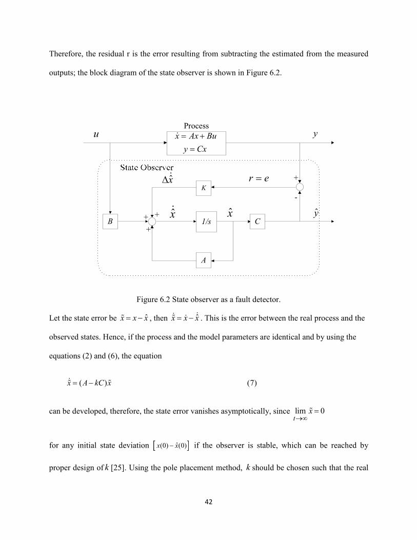
Therefore, the residual r is the error resulting from subtracting the estimated from the measured
outputs; the block diagram of the state observer is shown in Figure 6.2.
x Ax Bu
y Cx
= +
=
&
B
K
1/s C
A
y
y
u
+ x& x
r e=x∆&
+
+
-
+
Process
Figure 6.2 State observer as a fault detector.
Let the state error be ˆx x x= −% , then ˆx x x= − &&% & . This is the error between the real process and the
observed states. Hence, if the process and the model parameters are identical and by using the
equations (2) and (6), the equation
( ) (7)x A kC x= −&% %
can be developed, therefore, the state error vanishes asymptotically, since lim 0t
x→∞
=%
for any initial state deviation [ ]ˆ(0) (0)−x x if the observer is stable, which can be reached by
proper design of k [25]. Using the pole placement method, k should be chosen such that the real

43
part of [ ]( )−λ A kC be a negative, whereλ stands for eigenvalus. In our case the dimension of the
matrix A is one by one, therefore,
( )A kCR
kL
− =−
−
( ) 0I A kCλ − − =
( )A kCλ = −
Thus, we design k using the desired eigenvalue that meets the criteria. This criterion is to
make the observer more stable and fast to damp than the process can do. This would be achieved
if the eigenvalue is moved to the left of the s-plane.
Faults Lf act on the output error e according to the observer dynamics [ ]( )1
SI A kC− −−
. The
static deviation for a step-change 0Lf becomes,
[ ]( ) ( 0) ( )1
0lim ( ) (8)e t e s C A kC Lt
Lf s= = = − −−
→∞
and according to (8), it is clear that the gain k has an effect on the error’s value.
In this work, we have relied on the observer gain k to produce a residual. Because the residual
is a function of the observer gain, the residual value will be suppressed for high gain or
magnified for low gain. In such cases, the residuals do not provide accurate indication of fault
values. Reference [25] presents a way to avoid the effect of gain on residual by pre-multiplying
the residual with a factor 1( )I CA k−− . Then the final value of the residual will be,

44
( 0)1
0( ) (9)r e s CA LLf s= = = − −
In the next section we show how the proposed protection scheme responds to different fault
types
6.4. Application to Microgrid Protection
6.4.1. Observer-Based fault detector behavior with different kinds of faults
When three phase fault occurs in a protected zone, the three observers of those three phases
will have values in their residuals even if the microgrid is islanded and this is also applied for the
phase to phase faults. This value depends on the position of the fault in the protected zone. Since
the network impedances change in case of ground faults as shown in Figure 6.3, a separate
observer is designed based on the zero sequence impedance, voltages, and currents of the
protected zone and this observer is called Earth Fault Observer. Therefore, the design of earth
fault observer should consider the zero sequence impedance to find A and B.
Figure 6.3 Equivalent network of single line to ground fault.
To decouple the zero sequence currents and voltages, measurements should be taken from the
neutral point of the current transformers (only one end CT’s) and the open delta of the voltage

45
transformers (summation of the three phase voltages gives the same result) in both ends as
shown in Figure 6.4. The phase observers can detect the earth fault, but the earth fault observer
cannot detect the phase faults. The change in the network impedances makes the phase observers
to detect ground fault even if they are in the neighbor zones, but only the earth fault observer for
zone in fault detects that fault.
(a)
to P
has
e
obse
rver
s
(b)
Figure 6.4 Phase and earth fault observers connections of (a) Current transformers, (b) Voltage
transformers.
Therefore, the zone in fault could be recognized easily once its phase and earth fault observers
detected the ground fault in their residuals. By setting a margin time between phase and earth

46
fault observers, the ground fault can be detected and isolated before the phase observers can do.
This margin can be the same value for all zones and no grading time is necessary between zones.
For example, for earth fault observer of all zones, trip time can be adjusted to instantaneous
value and any larger values for phase observers.
Because the technique of the observer-based protection system relies on the error value,
residual of the earth fault observer can detect ground faults even if they are through high
impedance.
6.4.2. Minimum Measurements Placement
Finding the minimum number of measurement sensors that give enough fault information is a
challenge in this work. This guides to obtaining the observability of such a complex operation.
Although observability varies with the changes of the microgrid configuration, the minimum
measurement placement is still possible. Sources outages do not affect on the observability, but
feeders outages do. Therefore, taking feeders outages in consideration helps in placing current
and voltage measurements.
There will be an observer per phase of the protected zone and that helps for identifying the
fault type (phase to ground, phase to phase, and three phases fault). As a result, for each zone
there will be four observers, three for phase and one for earth fault. Therefore, all these observers
need input and output measurements.
Reference [26] describes a method of analyzing the observability and placing the phasor
measurement units (PMU) of a network. PMU’s are synchronized by global positioning system
(GPS), in addition, PMU’s provide voltage and current information. Each PMU can measure the
bus voltage and all currents of the connected lines to that bus. For the proposed protection
system it does not necessary to use PMU, any other mean of current and voltage measurements

47
are valid and no need to use GPS in the proposed system. In this work to reduce the system cost,
the ordinary (CT’s and VT’s) measurements of current and voltage can be used instead of
PMU’s which are more expensive.
For n-bus network, the placement is achieved as follows [26]:
min n
i ii
w x⋅∑
ˆ( ) 1f x ≥
1 , if a PMU is installed at bus =
0 , Otherwisei
ix
Where: wi is the cost of the PMU which installed at bus i and f(x) is a vector function, which
has non-zero entries if the related bus voltage can be solved using the given measurement set and
zero if cannot be solved.1 is a vector which all its entries are ones.
The next step is to estimate unmeasured quantities. Once the sensors are placed, the
unmeasured quantities can be estimated using Kirchhoff’s laws (KVL and KCL). Normally in
control design it is mandatory to find estimates of state variables that are not accessible by direct
measurement. For a linear system, state vector can be approximately estimated by constructing
an observer which can be built from outputs and inputs of the original system. The system that
has state vector of an nth order system with m independent outputs can be estimated using an
observer of order n-m [24]. In this paper there will be multi observer system which some of its
inputs (voltages) are not measured. Then, unmeasured voltage of any zone can be estimated as
follows:

48
1 1 2LV I Z V= +
Where,
LZ : is the line impedance,
1V : is the unmeasured voltage,
2V : is the measured voltage,
1I : is the line current.
In some cases not all currents can be measured and then will be estimated using KVL and
KCL.
6.4.3. Protecting Transformers Using Observer
Power transformers can be protected against internal faults using an observer technique. By
dealing with the transformer impedance and measuring primary or secondary current, and
primary and secondary voltages, any internal fault can be detected through the residual Figure
6.5.
Figure 6.5 One phase of a power transformer with zero shift angle.

49
To design the observer, voltage, current and impedance should be transformed to one side and
dealing with these quantities as in equation (1). Three phase transformers are designed in
different connections (vector group) and that produce phase shifts between primary and
secondary windings. This phase shift should be taken in consideration when transforming
voltage from side to another. If the transformer is fed or feeding through line, the line impedance
can be considered so that the observer could protect the line and the transformer together.
6.4.4. Multi-Zone Protection
For centralized protection system, multi input and multi output (mimo) state space
representation for the electrical system which represents branches of the microgrid system should
be constructed.
Figure 6.6 Multi observer system (Bank of observers).
It needs to find the differential equations that express the dynamic behavior of the electrical
power system; therefore, these equations are considered the infrastructure of mimo observer-
based protection system Figure 6.1. In this work the line currents are the states, hence in order to

50
reduce the number of current transformers in the microgrid, unmeasured states could be
estimated. For system inputs, end measured or estimated voltages can be implemented.
Multi-zone protection is constructed from number of single observers, describe all phases and
earth fault observers of protected zones, as found in section 6.3. Only the faulted phase and zone
would have value in its residual Figure 6.6.
6.5. Case Study
The observer-based protection system is tested using the IEEE 34 nod test feeder Figure 6.7.
There are distributed generators spread on the test feeder with voltage level of 24.9 kV, 60 Hz
and loads are distributed as well. All neutrals of generators are solidly grounded. The test feeder
is divided into zones as shown in Figure 6.7. Positive and zero sequence impedances used in this
test feeder are calculated using the formula:
s mZ Z Z+ = −
0 2s mZ Z Z= +
In this research the method of PMU placement which is explained using 7-bus in [26], can be
implemented on IEEE 34 bus distribution system to minimize the number of measurement
devices. This system can be divided into 17 zones, Figure 6.7; hence the required measurements
(current and voltage) should be positioned on 18 nodes which are the zones boundary nodes. A
connectivity matrix is constructed as follows:
1 if
= 1 if and are connected
0 otherwise,
k m
k mk mA=
The construction of A will be as the bus admittance matrix, but with binary entries. The matrix
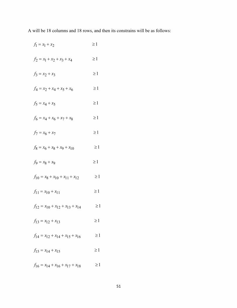
51
A will be 18 columns and 18 rows, and then its constrains will be as follows:
1 1 2 1f x x= + ≥
2 1 2 3 4 1f x x x x= + + + ≥
3 2 3 1f x x= + ≥
4 2 4 5 6 1f x x x x= + + + ≥
5 4 5 1f x x= + ≥
6 4 6 7 8 1f x x x x= + + + ≥
7 6 7 1f x x= + ≥
8 6 8 9 10 1f x x x x= + + + ≥
9 8 9 1f x x= + ≥
10 8 10 11 12 1f x x x x= + + + ≥
11 10 11 1f x x= + ≥
12 10 12 13 14 1f x x x x= + + + ≥
13 12 13 1f x x= + ≥
14 12 14 15 16 1f x x x x= + + + ≥
15 14 15 1f x x= + ≥
16 14 16 17 18 1f x x x x= + + + ≥

52
Figure 6.7 IEEE 34 node test feeder with protection zones.

53
17 16 17 1f x x= + ≥
18 16 18 1f x x= + ≥
Where, the operator “+” used as the logical “OR” and 1≥ means that at least one of the
variables appearing in the sum will be non-zero. To make bus 800 observable, for 1f at least one
PMU can be installed on bus 800 or 808 for minimum placement. For the minimum observability
of bus 808 ( 2f ), PMU can be installed on 800, 808, 810, or 816. It is clear from constrains that
common nodes are: 808, 816, 824, 854, 832, 858, 834, and 836, therefore, only eight PMU’s can
be placed on the IEEE 34 Bus system and will satisfy the observability condition.
A complete protection system is designed for all zones of the test feeder; each zone is
protected by three phase observers and one earth fault observer. All zones are examined for all
kind of faults and their stability and selectivity are checked too.
The definition of the contribution currents is explained in figure 6.8a which shows currents
that pass from the neighbor zones (H and M) toward faulted zone (K). To avoid the effect of
observer gain k, the equation (9) has been implemented on the observers’ residuals. Therefore,
the residuals values are more accurate and approximately equal to the short circuit current values
once a short circuit is applied Figure 6.8b.
For explanations, results that shown in this research are from the area starts from the node 800
to the node 824 which are marked with the zones: H (node 816 to 824), I (node 816 to 822), K
(node 808 to 816), L (node 808 to 810), and M (node 800 to 808). Faults are applied in the zone
K and the behavior of the other zones observers is checked.
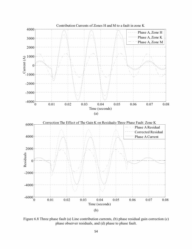
54
(a)
(b)
Figure 6.8 Three phase fault (a) Line contribution currents, (b) phase residual gain correction (c)
phase observer residuals, and (d) phase to phase fault.
0 0.01 0.02 0.03 0.04 0.05 0.06 0.07 0.08-4000
-3000
-2000
-1000
0
1000
2000
3000
4000
Time (seconds)
Curr
ent (A
)Contribution Currents of Zones H and M to a fault in zone K
Phase A, Zone H
Phase A, Zone K
Phase A, Zone M
0 0.01 0.02 0.03 0.04 0.05 0.06 0.07 0.08-6000
-4000
-2000
0
2000
4000
6000
Time (seconds)
Resi
duals
Correction The Effect of The Gain K on Residuals-Three Phase Fault: Zone K
Phase A Residual
Corrected Residual
Phase A Current

55
Figure 6.8 (Cont’d)
(c)
(d)
0 0.01 0.02 0.03 0.04 0.05 0.06 0.07 0.08-6000
-4000
-2000
0
2000
4000
6000
Time (seconds)
Resi
duals
Three Phase Fault in Zone K: Phase A Residuals
Zone H
Zone I
Zone K
Zone L
Zone M
0 0.01 0.02 0.03 0.04 0.05 0.06 0.07 0.08-5000
0
5000
Time (Seconds)
Resi
duals
Phase to Phase Fault in Zone K: Residuals
Phase A Zone K
Phase B Zone K

56
A three phase fault is applied in the zone K which is fed from the neighbor zones and only the
three phase observers belong to zone K can detect the fault Figure 6.8c. To examine the
protection system behavior with all kinds of fault a phase to phase fault is applied to the zone K
and only two faulted phase observers (phase a and b) of zone K detected the fault Figure 6.8d.
Simulation results have shown the observer's performance in loading case and fault case. The
simulated observers are only single phase observers. In loading case, the observers in all zones
cannot detect the load currents except if this load is located inside the zone.
(a)
Figure 6.9 Single line to ground fault in zone K, (a) currents in zones K and H, (b) Phase
residuals of zones K and H, (c) Earth fault residuals of zones K and H.
0 0.01 0.02 0.03 0.04 0.05 0.06 0.07 0.08-4000
-3000
-2000
-1000
0
1000
2000
3000
4000
Time (Seconds)
Curr
ent (A
)
Earth Fault Currents: Positive and Zero sequence Currents
+ Seq. in Zone K
+ Seq. in Zone H
0 Seq. in Zone K
0 Seq. in Zone H

57
Figure 6.9 (Cont’d)
0 0.01 0.02 0.03 0.04 0.05 0.06 0.07 0.08-5000
0
5000
Time (seconds)
Resi
duals
Phase A Residuals of Zone H and K in Case of Phase to Ground Fault in Zone K
Zone H
Zone K
(b)
(c)
0 0.01 0.02 0.03 0.04 0.05 0.06 0.07 0.08-6000
-4000
-2000
0
2000
4000
6000
Time (seconds)
Resi
duals
Earth fault Residuals of Zones H and K in Case of Phase to Ground Fault
Zone H
Zone K

58
Ground fault are more complicated than phase faults since the zero sequence impedance is
involved in the short circuit paths. Thus, phase observers can detect earth fault even if they are in
different zones Figure 6.9b, but only the earth fault observer of the zone K can detect the ground
fault in zone K. Earth fault is instantaneous and much faster than phase fault observers, so it will
trip before phase fault observers can do, Figure 6.9c.
Moreover, a double phase to ground is applied and the earth fault observer detected the fault
Figure 6.10.
Figure 6.10 Phase and earth fault residuals of zone K in case of double phase to ground fault in
zone K.
To check the behavior of the protection system during high impedance faults, a single line to
ground fault is applied through 10 ohm resistance. Figure 6.11 shows that the earth fault observer
can detect the fault even if it is through high impedance.
0 0.01 0.02 0.03 0.04 0.05 0.06 0.07 0.08-6000
-4000
-2000
0
2000
4000
6000
Time (seconds)
Resi
duals
Double Phase to Ground Fault in Zone K: Residuals
E/F Zone K
Ph A Zone K
Ph B Zone K

59
Observer-based protection system is applied on a power transformer which has the data in
table 6.1, which are taken from IEEE 34 node test feeder. The protection system is tested in
steady state and in single line to ground fault.
Figure 6.11 High resistance single line to ground fault in zone K.
In steady state, the observer shows stability and its residual has no value Figure 6.12a, while in
case of fault this residual has value Figure 6.12b.
Table 6.1 IEEE 34 node, transformer data
MVA Kv-high Kv-low R-% X-%
0.5 24.9 4.16 1.9 4.08
0 0.01 0.02 0.03 0.04 0.05 0.06 0.07 0.08-2000
-1000
0
1000
2000
Time (seconds)
Resi
duals
High Resistance Phase to Ground Fault in Zone K: Residuals
Zone K
Zone K

60
(a)
(b)
Figure 6.12 Observer’s behavior in case of: (a) steady state, (b) single line to ground fault at %50
of the primary winding of power transformer.
0 0.02 0.04 0.06 0.08 0.1-3000
-2000
-1000
0
1000
2000
3000
Time (seconds)
Curr
ents
(A
) and R
esi
dual
Power transformer Currents and Phase Residual in Steady State (No Fault)
Primary
Residual
Secondary
0 0.01 0.02 0.03 0.04 0.05 0.06 0.07 0.08-5000
0
5000
Time (seconds)
Curr
ent (A
) and R
esi
dual
Single Phase to Ground Fault in %50 of the Primary Winding
Primary
Residual
Secondary

61
The observer is also tested for out of zone (zone of protection) faults and shows stability in
case of phase faults but in case of out of zone earth faults, an earth fault observer is needed as
discussed in section 6.4.1. The zero sequence currents make effect in some transformers
connections (YY-grounded neutrals), but in delta connections the zero sequence currents are
filtered.
62
7. Discussion and Conclusion
Designing a protection system for microgrids is a trade between the cost and performance.
Microgrids are low voltage level and cannot use digital relays which are expensive to protect
them. Differential relay needs two ends current measurements and communication channels
between the two ends of the protected line; hence the use of differential protection is expensive
too. The configuration of microgrid is not constant and then big differences in short circuit
current values are following these changes. Directional overcurrent relays cannot be used since
there are large changes in short circuit levels when switching between grid-connected and
islanded mode. Grid-connected mode results in high short circuit levels while low short circuit
levels are experienced in islanded mode. The short circuit level in islanded mode may not pick
up the overcurrent relay. Therefore, microgrid needs an adaptive protection system which can
detect and isolate faults in either mode of microgrid operations. In addition, this system should
be cost effective.
A novel protection system for microgrids, which can be centralized or decentralized, is
developed using the state observer as a fault detector. The proposed protection system is easy to
construct mathematically. The state space representation is simple, it consists of one state which
is itself the output and then the residual can be found from the measured and estimated states. To
construct bank of observers, a communication system used for controlling microgrids can be
used to transfer voltage and current information. The use of minimum measurement placement
technique in the proposed protection system makes it cost effective. Measurement devices can be
reduced to the minimum number, and the cost could be reduced as well.

63
The system is simulated using ATP and good result was obtained. The system can detect the
phase and earth faults. Phase observers can detect phase and earth faults, but earth fault observer
detects only ground faults. Then, by adjusting the trip time of earth fault observer to a value less
than that of phase observer, the faulted zone can be identified and isolated. Earth faults are more
occurrence than phase faults, where statistics shown that earth faults are %90 of faults.
If the zone has loads inside it, this happens when some load nodes are skipped to reduce the
number of measurements, limitations (thresholds) must be considered in the phase observer's
residual so that the protection system would trip for values larger than the load. This situation
can be noticed only in phase observers.
In low voltage level of distribution systems it is not common to set up a backup protection
since it increases the system’s cost. For backup protection, if necessary, a backup observer can
be designed. This observer is covering two zones together and in fault case it detects and
confirms the faulted zone and phase.
Zone C
Load
Zone BZone A
Figure 7.1 A representation of backup zone (zone C).
64
Earth faults can be detected by phase observers of adjacent zones which can be considered as
backup protection for the faulted zone. Phase faults on the other hand cannot be detected by
observers of adjacent zones, and therefore a backup observer is needed. To design a backup
observer, two zones can be merged together as shown in Figure 7.1. Following the steps in
section 6.3, a backup zone is found. Loads that located in backup zone, their values can be
adjusted as limits (thresholds) in phase residuals of backup zone. A grading time must be set for
the backup zone so that it trips if one of main zones fails to detect or trip for a phase fault.
Backup observers can be connected to the same measurement devices of the main observers or
different if available.

65
REFERENCES

66
REFERENCES
[1] W. E. Feero, P. A. Reedsvill, D. C. Dawson, and J. Stevens, “Consortium for electric
reliability technology solutions white paper on protection issues of the microgrid concept.”
Transmission Reliability Program Office of Power Technologies, Assistant Secretary for
Energy Efficiency and Renewable Energy, U.S. Department of Energy, March 2002.
[2] E. Sortomme, G. J. Mapes, B. A. Foster, and S. S. Venkata, “Fault analysis and protection of
a microgrid,” in Proc. North Amer. Power Symp., Sep. 2008.
[3] J. L. Blackburn, “Protective relaying principles and applications.” Marcel Dekker Inc., New
York, 1987.
[4] J. M. Gers and E. J. Holmes, “Protection of electricity distribution networks,” IEE, London,
2004.
[5] AREVA, Network protection and automation guide. AREVA http://www.areva-td.com
[6] W. A. Elmore, “Protective relaying theory and applications,” Marcel Dekker Inc., New York,
1994.
[7] P. M. Anderson, “Analysis of faulted power systems,” The Iowa State University Press,
1981.
[8] A. F. Sleva, “ Protective relay principles,” CRC Press, New York, 2009.
[9] P. Barker, and R. W. De Mello, "Determining the Impact of Distributed Generation on Power
Systems: Part 1 Radial Power Systems," Presented at IEEE PES summer power meeting,
Seattle, WA, July, 2000.
[10] L. Xuan and S. Bin, "Microgrids - an integration of renewable ener gy technologies," in
Electricity Distribution, 2008. CICED. China International Conference on, pp. 1-7.

67
[11] J. A. P. Lopes, “Advanced microgrids as a component for active management of
distribution networks.” in Proc. 2009 IEEE Power Engineering Society International
Conference.
[12] J. Zhu, “Web services provide the power to integrate,” IEEE Power Energy Mag., vol. 1,
no. 6, pp. 40–49, Nov./Dec. 2003.
[13] R. H. Lasseter and P. Paigi, “ Microgrids: a conceptual solution” in proc. 2004 IEEE
Power Electronics Specialists Conference.
[14] E. Sortomme, S. S. Venkata, and J. Mitra. “Microgrid protection using communication-
assisted digital relays.” IEEE Trans. Power Delivery, vol.25, pp. 2789 - 2796, Oct. 2010.
[15] H. Al-Nasseri, M. A. Redfern, and R. O’Gorman.”Protecting micro-grid systems
containing solid-state converter generation.” in Proc. 2005 IEEE Future Power Systems
Conf.
[16] B. Li, Y. Li, and Z. Bo, A Klimek. “Design of protection and control scheme for
microgrid systems." in Proc. 2009 IEEE Universities Power Engineering Conf.
[17] F. Z. Peng, Y. W. Li and L. M. Tolbert.”Control and protection of power electronics
interfaced distributed generation systems in a customer-driven microgrid.” in proc. 2009
IEEE Power Engineering Society General Meeting.
[18] H. Nikkhajoei and R. H. Lasseter, “Microgrid protection,” in Proc. 2007 IEEE Power
Engineering Society General Meeting.
[19] L. T. G. Lima, N. Martins, and S. C. Jr.”Augmented state-space formulation for the study
of electric networks including distributed- parameter transmission line models.” IPST’99.
June 20-24, 1999, Budapest-Hungary.
68
[20] Y. Xu and J. Jiang, “Implementation of an observer-based fault detection scheme on a
lab-scale power system,” in Proc.1998 IEEE Electrical and Computer Engineering, pp. 573-
576 vol.2.
[21] M. Aldeen and F. Crusca. ”Observer-based fault detection and identification scheme for
power systems.” IEE Proc.-Gener. Transm. Distrib., Vol. 153, No. 1, January 2006.
[22] R. Isermann, “Fault-diagnosis systems: An introduction from fault detection to fault
tolerance.” Springer, Heidelberg, 2006.pp. 232-245.
[23] P. Frank, “Fault diagnosis in dynamic systems using analytical and knowledge-based
redundancy.” Automatica, 26(3):459-474, 1990.
[24] D. Luenberger. "An introduction to observers." IEEE Trans. Auto. Cont., vol. AC-16, p.
596, 1971.
[25] F. N. Chowdhury and W. Chen, “A modified approach to observer-based fault detection.”
22nd IEEE International Symposium on Intelligent Control Part of IEEE Multi-conference
on Systems and Control Singapore, October 2007.
[26] B. Xu and A. Abur. “Observability analysis and measurement placement for systems with
PMU’s.” Power Systems Conference and Exposition, 2004. IEEE PES, pages 943–946 vol.2,
Oct. 2004.
[27] M. Esreraig and J. Mitra.”An observer-based protection system for microgrids.” in
Proc.2011 IEEE Power Engineering Society General Meeting.