developing income proxy models for use by the usaid
TRANSCRIPT

DEVELOPING INCOME PROXY MODELS FOR USEBY THE USAID MISSION IN KENYA:
A TECHNICAL REPORT
David Tschirley and Mary Mathenge
Tegemeo Working Paper 7
November 2003
Tegemeo Institute of Agricultural Policy and DevelopmentP.O. Box 20498
00200 City SquareNAIROBI, KENYA
tel: 254-2-2717818fax: 254-2-2717819
email: egerton@tegemeo-org
�������������� �
Tegemeo Institute Of Agricultural Policy And Development

i
Table of Contents
I. Introduction . . . . . . . . . . . . . . . . . . . . . . . . . . . . . . . . . . . . . . . . . . . . . . . . . . . . . . . . . 1
II. Income Proxy Models: What Are They and How Can They Be Useful? . . . . . . . . . . 2A. Background . . . . . . . . . . . . . . . . . . . . . . . . . . . . . . . . . . . . . . . . . . . . . . . . . . . 2B. Monitoring or Impact Evaluation? . . . . . . . . . . . . . . . . . . . . . . . . . . . . . . . . . 3C. What Steps Are Needed to Develop an Income Proxy Model? . . . . . . . . . . . . 4D. Anticipated Time and Cost Savings from the Proxy Approach . . . . . . . . . . . . 6
III. The Tampa Data Set . . . . . . . . . . . . . . . . . . . . . . . . . . . . . . . . . . . . . . . . . . . . . . . . . . 7
IV. The Model Development Process . . . . . . . . . . . . . . . . . . . . . . . . . . . . . . . . . . . . . . . . 7A. Definition of Zones and Income Components . . . . . . . . . . . . . . . . . . . . . . . . . 7B. Types of Proxy Variables used in the Models . . . . . . . . . . . . . . . . . . . . . . . . . 8C. Improving the Zonal Models . . . . . . . . . . . . . . . . . . . . . . . . . . . . . . . . . . . . . 10
V. Model Performance . . . . . . . . . . . . . . . . . . . . . . . . . . . . . . . . . . . . . . . . . . . . . . . . . . 10A. Internal Performance Evaluatio . . . . . . . . . . . . . . . . . . . . . . . . . . . . . . . . . . . 10
How well do the models predict total income levels over space? . . . . . . . . . 11How well do the models predict income sources nationally? . . . . . . . . . . . . 13How well do the models predict rates and depth of poverty? . . . . . . . . . . . . 13How well do the model results perform in bivariate (tabular) analyses? . . . 14How well do the model results perform in multivariate analyses? . . . . . . . . 16
B. External Performance Evaluation . . . . . . . . . . . . . . . . . . . . . . . . . . . . . . . . . 16C. Conclusions from Model Evaluation . . . . . . . . . . . . . . . . . . . . . . . . . . . . . . . 17
VI. Using the Models . . . . . . . . . . . . . . . . . . . . . . . . . . . . . . . . . . . . . . . . . . . . . . . . . . . . 18
ANNEXES
ANNEX PAGE
A. Cost Comparison, Proxy Vs. Full Income Survey . . . . . . . . . . . . . . . . . . . . . . . . . . 20
B. Income Proxy Questionnaire for Tampa Models . . . . . . . . . . . . . . . . . . . . . . . . . . . . 22
C. Enumerator Manual for Proxy Survey . . . . . . . . . . . . . . . . . . . . . . . . . . . . . . . . . . . . 33
D. Full Model Results . . . . . . . . . . . . . . . . . . . . . . . . . . . . . . . . . . . . . . . . . . . . . . . . . . . 40
E. Procedures for Generating Income and Income Component Estimates UsingSpss/windows Syntax File . . . . . . . . . . . . . . . . . . . . . . . . . . . . . . . . . . . . . . . . . . . . 113

ii
List of Tables
TABLE PAGE
1. Indicative Time and Cost Savings of Proxy Approach Compared to Full IncomegSurvey, Each Covering 1,500 Households . . . . . . . . . . . . . . . . . . . . . . . . . . . . . . . . . 6
2. Explanatory Power (R2) on Total Income, by Zone . . . . . . . . . . . . . . . . . . . . . . . . . 11
3. Mean of Actual and Predicted Incomes, and Income Ranking, by Model, by Zone andDistrict . . . . . . . . . . . . . . . . . . . . . . . . . . . . . . . . . . . . . . . . . . . . . . . . . . . . . . . . . . . . 12
4. Explanatory Power (Pseudo-R2) on Income Components, National . . . . . . . . . . . . . 13
5. Income Levels and Poverty Measures by Zone, Actual and Predicted Data . . . . . . . 14
6. Income Levels and Shares by Source, and Wealth Indicators by per capita IncomeQuintile, by Calculated and Predicted Income . . . . . . . . . . . . . . . . . . . . . . . . . . . . . 15
7. Determinants of Household per capita Income, Actual Values Compared to Model-Generated Values (Linear regression results after controlling for village level effects) . . . . . . . . . . . . . . . . . . . . . . . . . . . . . . . . . . . . . . . . . . . . . . . . . . . . . . . . 16
8. Comparison of Relationship Between Headcount Poverty Index and HouseholdDemographic Variables in Welfare Monitoring Survey (WMS) and Tegemeo/MSUData, Using WMS Definition of Adult Equivalent and Based on Income/AE . . . . . 18
Figures
1. Overview of Process to Develop and Apply Income Prediction Models . . . . . . . . . . 4

1 See, for example, Daniels 1999; Glewwe 1990; Glewwe and Kanaan 1989; Grosh and Baker 1995;Hentschel et al. 1998; Jalan and Ravallion 1999; Little 1997; Minot 2000; Morris et al. 1999; Ravallion andLokshin 1999; Riely et al 1999; Rose 2000; Rose and Tschirley 2000; Sahn and Stifel 2000a; Sahn and Stifel2000b; Swindale and Ohri-Vachaspati 1999; Takasaki and Barham 2000l; Wolfe and Frongillo 2000; WorldBank 2001;
1
Developing Income Proxy Models for use by the USAID Mission in Kenya:A Technical Report
By
David Tschirley and Mary Mathenge
I. Introduction
Governments, donors, and NGOs in developing countries spend billions of dollars every yearon efforts to improve the well-being of rural households. Most of these interventions havethe ultimate goal of reducing poverty, and many include specific objectives of increasinghousehold incomes from specific activities such as microenterprise, cash cropping, foodcropping, or livestock. Since an accurate assessment of these outcomes is costly and time-consuming, much research has attempted to identify simple indicators which are correlatedwith the variables of interest.1 The income proxy models developed in Kenya are one methodin this large and expanding toolbox of low cost approaches to monitoring otherwise complexindicators of household welfare.
The work in Kenya builds on and improves methods developed earlier in Mozambique(Tschirley, et al. 1999) and applied by NGOs there. The purpose of the models as currentlydeveloped in Kenya is to provide donors, government agencies, and other interestedorganizations with a low cost method to generate estimates of total household income, brokendown by eight different income sources. In addition to generating estimates of mean incomeson a geographically disaggregated basis for monitoring purposes, the model results will beuseful for a series of basic descriptive analyses to be described below.
This paper details the specific procedures utilized to develop the income proxy method forthe USIAD/Kenya mission, reports on the performance of the method, and brings together inone place each part of the package needed to implement the method. The next sectionprovides general background on income proxy methods; section III reports briefly on theTegemeo/MSU Tampa full income survey that formed the basis for development of the proxymethod; section IV provides details on model development, including definition of incomecomponents, the types of proxy variables tested, and the performance of the models; sectionV assesses model performance, and section VI touches on how the models can be used. Acompanion document (Developing Income Proxy Models for Use by Title II-funded NGOs inKenya: A Technical Report for NGOs and USAID/Kenya) provides similar documentationfor the modeling effort undertaken with NGOs.

2 If desired, the models could be developed to return per capita household income, as opposed to totalhousehold income.
2
�Yi�ai�bi1Xi1�bi2Xi2�...�binXin�ei
�Y��C
i�1
�Yi
II. Income Proxy Models: What Are They and How Can They Be Useful?
A. Background
An income proxy model is one part of a package of procedures that NGOs, donors,governments, or research institutions can use to monitor rural household income and incomecomponents using easy-to-collect proxy variables. The model is a set of algebraic equationsthat relate these proxy variables to components of income:
where,
is estimated income from component i, �i
ai is a constant (or intercept) term for income component i, bi1 ... bin are the coefficients (fixed numbers) that quantify the relationship of each
proxy variable to income component i, Xi1 ... Xin are the selected proxy variables for income component i, andei is a random error term.
Taken together, the various components in the model sum to total household income:2
where,
is estimated total income,�is estimated income from component i, and�
iC is the number of income components.
These algebraic relationships are developed using standard "ordinary least squares"econometric techniques applied to a household data set which contains detailed data onhousehold incomes and the proxy variables. Once this detailed data set is collected and themodel is estimated, one needs only to collect the proxy variables to obtain estimates ofincome components and total household income. These simple proxy surveys will typicallybe conducted once a year, or however often the institution wishes to track household income. The much more detailed and time consuming income survey needs to be done once at thebeginning of the project cycle and preferably again at the end of the cycle for validation

3 For a good introduction to this topic, see Ravallion, Martin (1999). "The Mystery of the VanishingBenefits: Ms. Speedy Analyst’s Introduction to Evaluation". Policy Research Working Paper ..., Washington,D.C., World Bank.. This can be downloaded from the web by going to www.worldbank.org/research/,choosing "poverty", then searching for "Ravallion" under "Policy Research Working Papers".
3
purposes. The complete package which defines the income proxy methodology includes 1)sampling guidelines for the periodic proxy surveys, 2) a model questionnaire for thesesurveys, 3) the set of econometric models relating the proxy variables to household incomeand income components, 4) SPSS/Windows syntax files based on these models that use theproxy data to generate the quantitative income estimates, and 5) a manual for operating thepackage.
The usefulness of an income proxy methodology derives from the importance of householdincome as an objective of development activities: an important overall development goal innearly every developing country is the reduction of poverty and improvement in the incomesand well-being of rural households. Thus, measurement of household income is one logicalchoice for monitoring the effects of policies and programs oriented towards accomplishingthis goal.
B. Monitoring or Impact Evaluation?
The econometric models in the income proxy methodology are designed to capture theassociation between income and the proxy variables, and to return as accurate a prediction aspossible. As such, they can be used directly to monitor the types of economic activities thathouseholds engage in, and the incomes they derive from these activities. The modelsthemselves are not designed to allow conclusions regarding cause and effect; to use thesemodels for impact evaluation (for example, to measure the impact of an NGO’s agriculturalproduction and marketing assistance on agricultural and overall household income), theyneed to be integrated into an overall approach which includes the following elements:
� A sampling design that distinguishes between participants (the target population for theintervention being evaluated) and non-participants (the non-target population),
� A baseline survey conducted prior to the beginning of the intervention, distinguishingbetween likely participants and likely non-participants,
� The collection of complementary data regarding the physical, economic, and socialenvironment of the participating and non-participating households.
It is beyond the scope of this paper to go into detail on impact evaluation;3 suffice it to saythat, within such an integrated approach, use of income proxy models can allow morefrequent monitoring (because it will be less costly and less time consuming), provide a richerset of monitoring results covering the range of the households’ economic activities, andreduce the cost of the impact evaluation.

4
Phase II — Develop prediction model
Figure 1. Overview of Process to Develop and Apply Income Prediction Models
C. What Steps Are Needed to Develop an Income Proxy Model?
Figure 1 provides an overview of the process for developing and utilizing an income proxymodel. Once the original, detailed data are collected and the prediction model is developed(Phases I and II), one need apply only Phases III & IV for the remaining years of theprogram before collecting a new full data set to re-estimate the prediction model and performa full evaluation of the program.
To develop the model, the analyst must work closely with users to:
1. Understand the design and operation of the interventions that are being monitored,and the economic environment where they are being implemented. The analystsdeveloping the model need this type of information to define a set of econometricmodels that are meaningful for the user and that can be estimated with acceptableaccuracy with proxy variables.
2. Define a relevant and feasible breakdown of income components to be modeled. The preferred definition will depend primarily on the types of economic activities which

5
are most important in the area where the intervention is taking place. For example, in apastoral area with little crop production, the latter may be grouped into a singlecomponent, while livestock activities might be broken into several components. In anarea of heavy cropping activities where livestock is less important, the reverse mighthold.
3. As much as possible, anticipate the proxy variables that will be used to model eachcomponent. While not every proxy variable can be defined prior to the data analysis,many can be, and identifying a comprehensive list of probable and possible proxiesahead of time will improve the modeling results. As in the definition of incomecomponents, there will be substantial similarities in the definition of these variablesacross users, but if the income components are not identical, neither will the proxyvariables be.
4. Design and conduct a detailed income survey that will provide the data to estimate themodels. In the case of the models developed for USAID/Kenya, this survey wasconducted by Tegemeo/MSU in 2000, and included design elements that anticipated thedevelopment of these models.
5. Estimate the models. The data must be entered, cleaned, organized, and then analyzedto develop the prediction models.
6. Develop a model questionnaire for the proxy surveys. Defining the models involvesdefining the most efficient set of proxy variables for each income component. Once thisis done, a questionnaire is designed to collect just these proxy variables in future years. These questionnaires consist almost entirely of yes/no questions, with quantification of alimited number of variables. Thus, these questionnaires are much shorter, the interviewsare shorter and easier to conduct, and the data are much easier to enter and clean than afull income survey. See Annex B for the proxy questionnaire designed for the USAIDMission models.
7. Develop a data processing routine to convert the proxy variables into estimates ofincome components and total income. Tegemeo/MSU have developed a SPSS/Windowssyntax file that performs this function. It is available in electronic version upon request.
D. Anticipated Time and Cost Savings from the Proxy Approach
Table 1 shows estimated time and cost savings of using a proxy approach as opposed to a fullincome survey. The numbers in the table are derived from Annex Table A1, which is basedon Tegemeo’s experience with the full income survey in 2000 and the proxy survey in 2002,and on NGOs’ experience with the proxy method in 2003. The time and cost savings of theproxy approach come in all phases of the work. Questionnaire design for Phase III is limitedto reviewing the model proxy questionnaire and making any small changes required for thespecific circumstances (without, of course, changing the actual data to be gathered nor itsstructure). Tegemeo experience in 2002 and NGO experience in 2003 suggests that aninterview for the simple proxy survey takes one-quarter or less time than an interview for thefull income survey; total time savings in data collection will be less than this due to the fixed

4 Though initial results for the proxy method are produced instantaneously by running the syntax filealready created, results have to be reviewed for consistency and checked for outliers. This process took oneweek at about 50% time for a Senior Analyst on the NGO survey of 1,200 households.
6
Item Estimated Cost (US$) Estimated Elapsed Time(weeks)
Full Survey Proxy Method Full Survey Proxy Method
Questionnaire design 2,302 307 3.0 0.40
Data collection 43,362 23,412 7.0 7.00
Post-coding and data entry 4,721 1,180 3.0 0.75
Data cleaning 10,468 2,617 6.0 1.50
Data analysis 27,000 1,709 13.0 1.00
Total 87,853 29,225 32.0 10.65
... of which Analysts 33,416 6,231
Table 1. Indicative Time and Cost Savings of Proxy Approach Compared to FullIncome Survey, Each Covering 1,500 Households
costs of reaching villages and finding households within them, which is the same for eachsurvey. The largest time savings come after data collection: due to lower data volume andsimpler variables, post-coding and cleaning of the proxy data take about one-quarter or lesstime than the full survey, while data analysis takes about one week, compared to an estimated3 months on a full income survey.4
On this basis, we conservatively estimate that the proxy survey reduce monetary costscompared to a full income survey by approximately 2/3, and elapsed time (from thebeginning of the exercise to having needed results from the data) by a similar amount, fromover 30 weeks to about ten weeks. Analyst time is especially scarce in most organizations,and these overall figures mask the greater savings of their time; we estimate these savings tobe over 80% (Table 1, based on Annex Table A1).
The proxy surveys of Phase III need be conducted only once a year, or however often theinstitution wishes to track household income and income sources. For validation purposes,the full income survey of Phase I survey should be conducted again at a later time and, ifneeded, the prediction models should be recalibrated.
It should be noted that these time and cost savings are achieved due to the up-frontinvestment in developing the proxy models, the proxy questionnaire, and the processingroutine to convert proxy variables into income estimates. These activities are all additionalto what would normally be done with an income survey. Based on experience to date inKenya, this process takes about one and one-half months of full-time work for an Analyst

5 See Argwings-Kodhek et al (1999), "How Can Micro-level Household Information Make aDifference for Agricultural Policy Making? Selected Examples from the KAMPAP Survey of SmallholderAgriculture and Non-Farm Activities for Selected Districts in Kenya," for more background on the methodsused in the Tampa Survey.
7
and Senior Analyst. Thus, to be cost effective, and considering that a full income surveyprovides a richer data set for policy analysis, we suggest that the method be adopted only if itwill meet critical M&E needs during at least two years, and preferably more.
III. The Tampa Data Set
The Tegemeo Institute "Tampa" survey, a joint undertaking by Tegemeo Institute/EgertonUniversity and Michigan State University, contains about 1,500 households and is designedto be representative of 24 purposively chosen agricultural districts of the country. Thesedistricts were chosen to be representative of all but the non-marginal, largely pastoral, areasof the country.5 For the development of the income proxy models, data from Turkana andGarissa districts were eliminated, as were several cases considered to be outliers. In all,1,392 cases were used in this analysis.
Because the Tampa sample was not fully randomized, and because the sample size wasrelatively small when compared to national surveys such as the Welfare Monitoring Survey,geographical breakdowns in this report are presented at a fairly aggregated level - four zones,each comprising more than one province. Breakdowns below this level, for example in Table3 at the district level, are legitimate for internal evaluation of the income proxy models, butshould not be compared to results from WMS surveys at that level.
IV. The Model Development Process
A. Definition of Zones and Income Components
To develop the income prediction models using the Tampa data set, we first divided thecountry into four zones, each of which would have its own models. These zones were basedloosely on agro-ecological conditions, and on the need to have sufficient sample size in eachzone to ensure adequate degrees of freedom for the analysis. The zones and Tampa samplesizes are
� Coastal & Eastern, 240 households� Western Lowlands & Transitional, 343 households� High potential maize zone, 399 households� Western & Central highlands, 410 households
These zones are meant to be representative of the non-marginal agricultural areas of thecountry; they exclude the northern arid zone and the Marginal Rain Shadow, which togetherhad only 120 households in the Tampa sample.
After defining the four zones for modeling purposes, it was necessary to divide householdincome into a workable number of meaningful components. Conceptually, income can be

8
broken into a very large number of components; the specific components chosen should be afunction of their relevance for understanding rural households and the rural economy, and theaccuracy with which they can be predicted. For a given level of desired accuracy in theestimate of total income, estimating more income components will require the collection ofmore proxy variables. At some point, the number of variables collected becomes excessivegiven the fundamental objective of the proxy approach, which is to reduce the cost ofobtaining defensible estimates of household income. The analyst’s challenge is to define aset of components which strikes a balance between accuracy, richness of information, and theamount of data collection and processing required.
After considering these issues, and based on a desire for the models to generate insights onthe importance of farm vs. off-farm incomes and, within farm income, to highlightdifferences in incomes from marketing and in-kind incomes from home consumption, wechose eight income components:
1. retained cereals & tubers2. sold cereals & tubers3. retained fruit & vegetables4. sold fruit & vegetables5. "industrial" crops (all crops other than cereals & tubers and fruits &
vegetables)6. all livestock and livestock products7. informal off-farm incomes (informal wage labor and microenterprise
activities, including jua kali)8. formal wage labor (salaried labor) & remittances
Summing the values of the eight components gives total household income. Across the fourzones, these eight components required 32 models, which we call the zonal models.
B. Types of Proxy Variables used in the Models
In attempting to estimate each of these components, emphasis was placed on identifyingproxy variables that would be straightforward to collect and process, and which had stronglogical and empirical links to the level of income from the component. Seven general typesof variables were used in the models:
� Measures of the intensity of involvement in the activity. Measures of intensity varied bycomponent, but for the agricultural components typically included the number of itemswithin the category that the household produced (for example, the number of food cropsthat the household cultivated), and the number of items that it sold (or whether it soldany, or not). For off-farm components, this set of variables generally included thenumber of people involved in the activity (informal off-farm or salaried labor &remittances), and the number of months in the year in which someone was involved. This set of variables also included indicators of the specific nature of involvement in theactivity (e.g., what general type of wage labor, or what type of informal businessactivity)

6 This proxy variable is generated from a regression using simple yes/no responses to the ownership ofa set of 15 assets. Thus, it is not necessary to collect number owned and value of a large set of assets to obtainthis variable.
9
� Production function variables. These were the same for all cropping activities: totalacres owned (rather than the more difficult to collect acres in specific crops), use offertilizers (yes/no), and hiring of labor (yes/no).
� Selected quantitative variables. Quantitative variables are more complex to collect andprocess than typical proxy variables, but are needed because production levels canfluctuate substantially from year-to-year based on rainfall and other factors. Byquantifying the production of the most important food crop and cash crop, thesequantities can themselves proxy for yield levels of other crops within their category. This should substantially improve the performance of the method over time. We usedfive quantitative variables in the models: the quantity produced of the "most important"food crop for home consumption, the quantity produced of the food crop that gave mostsales income, the quantity produced of the industrial crop that gave most sales income,the quantity produced of the "most important" fruit or vegetable for home consumption,and the quantity produced of the fruit or vegetable that gave most sales income. Byallowing the households to specify their "most important" crop in these variouscategories and quantifying that, the models should do a good job capturing the effect ofchanging cropping patterns in rural areas o the country.
� Farmer assessment of the crop harvest. This set of variables includes adverse eventvariables for the crop production components, such as damage from several sources(yes/no), the number of crops that were completely lost due to any problem, and thefarmer’s overall assessment of the quality of the year’s harvest. These variables willhelp the models capture year-to-year changes in weather and pest problems.
� Household characteristics, such as schooling of the head of household, whether thehousehold is female-headed, and the estimated value of non-land assets held by thehousehold.6
� Household ranking of the relative importance of the income source compared to othersources.
� Interaction terms. We made very liberal use of interaction terms to get maximum valueout of the variables used. For example, by interacting the number of months that anyonein the household earned income from any informal off-farm activity (a simple yes/noquestion) with yes/no indicators of the type of activities that the household was involvedin (also yes/no questions), we obtained a proxy for the number of months worked in thatspecific activity; this variable, and others like it, was quite useful in several of themodels.

10
C. Improving the Zonal Models
Evaluation of the performance of the 32 zonal models revealed that, while they performedquite well predicting income levels from the eight sources in each zone, they substantiallyunderestimated the importance of off-farm incomes for the lowest income households. Thesemodels estimated the off-farm income share (the sum of components 7 and 8) of the poorest20% of households at only 9%, while the actual income data showed the share to be 33%. Given the importance for policy purposes of knowing the relative importance of farm andoff-farm incomes for rural households, especially the poorest, we considered thisunderestimate to be a serious problem. To correct this shortcoming, we chose to useinformation about expected income levels (from the zonal models) to estimate twoconditional models:
1. Re-estimate each of the eight component models by quintile of predictedincome from that component (predicted from the zonal models). For example,income from retained cereals and tubers was estimated for each of the fivequintiles of predicted income from that source. This procedure generated 40models (5 quintiles for each of 8 components), and are called the componentincome quintile models..
2. Re-estimate each of the eight component models by quintile of estimated totalper capita income from the zonal models. In this approach, each of the eightcomponents was estimated for each of the five quintiles of predicted totalhousehold per capita income. This procedure also gave a total of 40 models,which we refer to as the per capita income quintile models.
We expected these two conditional approaches to help resolve the problem we had identifiedbecause they estimate models for groups of households that are relatively homogeneous interms of incomes (the five quintile groupings based on predicted income levels from thezonal models). If the zonal models predict incomes with substantial accuracy (which theydo), then the conditional models are very likely to provide better estimates than the zonalmodels, as will be seen in the next section.
V. Model Performance
A. Internal Performance Evaluation
Our evaluation of the models’ performance will focus primarily on checks internal to theTampa data set - how well the models predict income and income shares as calculated in thatdata set, and examined from a number of perspectives. Specifically, we will look at fourdimensions of performance:
• How well the models predict income levels over space, • How well they predict income sources nationally, • How well they predict poverty rates and depth over space, • How well they perform in tabular analysis by income quintile, and• How well they perform in multivariate analysis.

7 Full model results can be found in Annex D.
11
Zone
R-Squared (proportion of total variation in hh income
explained by model)
Zonal Models ComponentIncome Quintile
Models
Per capitaIncome Quintile
Models
Coastal & Eastern 0.858 0.860 0.860
Western Lowlands & Transitional 0.890 0.874 0.885
High potential maize zone 0.814 0.843 0.848
Western & Central highlands 0.867 0.876 0.875
National 0.850 0.863 0.866
Table 2. Explanatory Power (R2) on Total Income, by Zone
In all these internal analyses, the benchmark for comparison will be data as calculateddirectly from the Tampa data set.
How well do the models predict total income levels over space?7
Table 2 shows that each of the models explain about 85% of the variation around the meannationally and in each of the four zones. The two conditional models perform slightly betterin this regard, with most of the improvement coming in the High Potential Maize Zone.
Table 3 compares predicted to actual values of mean income for each of the four zones andthe 21 districts in the analysis, calculates the errors for each model, and shows the ranking ofzones and districts that each model gives. As expected, the zonal models provide moreaccurate estimates of incomes at the zone level, though errors are small in all three models. All models correctly rank the zones. When examining the results at district level, the secondconditional model, based on quintiles of expected per capita income, performs substantiallybetter than the other two, ranking 12 of the 21 districts correctly, and 18 either correctly orwithin one place. The other two models rank only 7 districts correctly, and have more largeerrors in both ranking and mean income than the second conditional model.

12
Zone/District
Calculated percapita Income
Estimated per capita Income
Level(Ksh)
Rank Zonal Models Component IncomeQuintile Models
Per capita IncomeQuintile Models
Level(Ksh)
%Error
Rank
Level(Ksh)
%Error
Rank Level(Ksh)
%Error
Rank
Coastal & Eastern 15,874 3 15,781 -0.6% 3 16,068 1.2% 3 15,475 -2.5% 3
W. Lowlands & Trans. 12,703 4 12,766 0.5% 4 12,633 -0.5% 4 12,801 0.8% 4
High potential mz zone 20,647 2 20,568 -0.4% 2 20,540 -0.5% 2 20,568 -0.4% 2
W. & C. Highlands 23,292 1 23,490 0.9% 1 23,727 1.9% 1 23,569 1.2% 1
National 18,645 18,681 0.2% 18,760 0.6% 18,660 0.1%
Siaya 7,412 21 8,094 9.2% 21 7,943 7.2% 21 7,620 2.8% 21
Kisumu 7,887 20 7,672 -2.7% 20 7,673 -2.7% 20 7,813 -0.9% 20
Taita Taveta 8,748 19 10,491 19.9% 19 11,071 26.6% 19 9,644 10.2% 19
Kilifi 10,228 18 9,277 -9.3% 15 9,918 -3.0% 16 10,247 0.2% 16
Vihiga 11,575 17 13,642 17.9% 17 13,681 18.2% 12 12,902 11.5% 18
Mwingi 12,748 16 11,632 -8.8% 16 12,193 -4.4% 15 12,199 -4.3% 13
Kisii 12,951 15 13,356 3.1% 13 14,082 8.7% 14 14,126 9.1% 15
Kitui 15,318 14 13,247 -13.5% 18 13,979 -8.7% 18 14,910 -2.7% 17
Kakamega 16,864 13 17,026 1.0% 12 16,667 -1.2% 13 17,010 0.9% 14
Trans Nzoia 17,325 12 16,419 -5.2% 14 17,478 0.9% 17 17,918 3.4% 12
Muranga 17,630 11 18,402 4.4% 11 18,452 4.7% 11 17,362 -1.5% 10
Machakos 17,973 10 19,787 10.1% 9 20,861 16.1% 10 17,967 0.0% 11
Makueni 18,434 9 18,458 0.1% 10 19,548 6.0% 9 19,442 5.5% 9
Bungoma 19,682 8 21,612 9.8% 6 21,461 9.0% 7 21,105 7.2% 8
Kwale 20,472 7 19,247 -6.0% 7 19,923 -2.7% 8 19,602 -4.3% 7
Nakuru 20,924 6 20,519 -1.9% 5 20,149 -3.7% 5 19,298 -7.8% 5
Uasin Gishu 21,050 5 21,493 2.1% 8 19,317 -8.2% 6 21,211 0.8% 6
Narok 22,456 4 20,463 -8.9% 3 20,599 -8.3% 3 21,088 -6.1% 4
Bomet 30,029 3 27,645 -7.9% 4 26,845 -10.6% 4 27,773 -7.5% 3
Nyeri 31,994 2 31,167 -2.6% 1 31,081 -2.9% 1 31,104 -2.8% 2
Meru 36,418 1 39,487 8.4% 2 38,665 6.2% 2 37,450 2.8% 1
Table 3. Mean of Actual and Predicted Incomes, and Income Ranking, by Model, by Zone and District

8 This current analysis is an internal evaluation of the income proxy method’s results, and is not meantto compare these results to those from the Ministry of Planning and Finance (2000a and 2000b). See later in thereport for a brief comparison of the two data sets.
13
Table 4. Explanatory Power (Pseudo-R2) on Income Components, NationalIncome Component Zonal Models Component
Income QuintileModels
Per capitaIncomeQuintileModels
Retained cereals and tubers .859 .848 .857
Sold cereals and tubers .928 .926 .938
Industrial crops .976 .978 .976
Retained fruits and vegetables .631 .651 .722
Sold fruits and vegetables .850 .818 .858
Livestock .730 .748 .786
Informal off-farm .592 .624 .653
Salaries & remittance .749 .767 .781
How well do the models predict income sources nationally?
From Table 4, we see that the models are most effective predicting income components fromsold agricultural production (sold cereals and tubers, industrial crops - nearly all of whoseproduction is sold - and sold fruits and vegetables). The models are least effective with thetwo off-farm income components, but still predict over 70% of the variation across the two. Conditional model 2 (with component regressions conditional on expected total per capitaincome) outperforms the other two models in 7 of the 8 components.
How well do the models predict rates and depth of poverty?
For this analysis, we used a relative poverty line equal to the 30th percentile in the incomedistribution, i.e., the bottom 30% of the sample was defined as poor.8 We calculate theheadcount index to measure the rate of poverty, and the Thorbecke-Greere poverty gap with� = 1 to measure the depth of poverty. Both are standard indicators used in poverty analysis. All four models rank the zones correctly in terms of headcount index and poverty gap, andaccurately reflect the relative differences between zones in these measures (Table 5). Thereis little to distinguish the models’ performance on the headcount index, while the secondconditional model performs best in poverty gap analysis, with an error less than or equal tothe other two models in every zone.

14
ZoneHeadcount Index Poverty Gap (alpha=1)
Calcul-ated
ZonalModels
ComponentIncomeQuintileModels
PerCapitaIncomeQuintileModels
Calcu-lated
ZonalModels
ComponentIncomeQuintileModels
PerCapitaIncomeQuintileModels
W. Lowlands& Transitional
0.46 0.43 0.44 0.41 0.23 0.20 0.20 0.22
Coastal &Eastern
0.32 0.32 0.28 0.33 0.12 0.14 0.09 0.11
High potentialmaize zone
0.24 0.19 0.19 0.20 0.10 0.08 0.08 0.08
W. & C.highlands
0.21 0.21 0.16 0.19 0.09 0.11 0.07 0.07
Table 5. Income Levels and Poverty Measures by Zone, Actual and Predicted Data
How well do the model results perform in bivariate (tabular) analyses?
To date, there is little to distinguish the models in terms of their performance, with all fourpredicting very large shares of the variation in household incomes and income components,and performing well also in the headcount index and poverty gap analyses at the zonal level. The differences in performance in the models emerge much more clearly when we use theirpredicted values to conduct tabular and multivariate analyses. In Table 6 we presentexamples of tabular analysis that could be done with the original, calculated income levels,and with the predicted income levels from the three models we have specified. For eachmodel, we rank households into quintile of per capita income, then examine income shares,the value of non-land assets, and the amount of cultivated land for each quintile. Note that,in the results for the three models, the value of non-land assets is itself a proxy variable basedon a regression of simple yes/no responses to the ownership of a set of 15 assets against thecalculated total value of over 40 assets. This variable will be generated directly from thesimple proxy data collected in the Phase III survey.
The table shows that all three models perform relatively well estimating income shares in allbut the lowest per capita income quintile. In this lowest quintile, the zonal models badlyunderestimate the share of income from off-farm, estimating this share at 9% compared tothe 33% share indicated by the actual data. Both conditional models perform much better inthis regard, estimating the off-farm share at 34% and 31%. Given the importance from apolicy perspective of knowing with some accuracy the importance of farm vs. off-farmincomes for rural households, we consider the superior performance of the conditionalmodels in this regard to be a key point in their favor.

15
Table 6. Income Levels and Shares by Source, and Wealth Indicators by per capita Income Quintile, by Calculated and Predicted Income
Per CapitaIncomeQuintile
Data Total percapita
Income (Ksh)
Crop Agriculture Livestock Off-farm Non-landAssets4
(Ksh)
Cultivated Land
(ha)Level(Ksh)
Share Level(Ksh)
Share Level(Ksh)
Share
1 Actual 2,962 1,614 0.54 371 0.13 977 0.33 53,894 3.2
From model 11 2,696 1,681 0.62 785 0.29 230 0.09 51,982 3.2
From model 22 3,491 1,682 0.48 625 0.18 1,184 0.34 62,182 3.0
From model 33 3,403 1,761 0.52 602 0.18 1,040 0.31 55,295 3.3
2 Actual 7,503 3,626 0.48 1,216 0.16 2,661 0.35 103,786 4.6
From model 1 8,004 3,449 0.43 1,772 0.22 2,782 0.35 109,660 4.4
From model 2 8,217 3,467 0.42 1,547 0.19 3,203 0.39 104,654 4.6
From model 3 8,069 3,626 0.45 1,627 0.20 2,816 0.35 105,135 5.0
3 Actual 13,016 5,767 0.44 2,414 0.19 4,835 0.37 105,261 4.5
From model 1 14,091 6,256 0.44 2,613 0.19 5,222 0.37 118,297 4.9
From model 2 13,688 6,118 0.45 2,570 0.19 5,000 0.37 109,768 4.8
From model 3 13,429 5,750 0.43 2,440 0.18 5,238 0.39 115,413 4.2
4 Actual 20,828 9,545 0.46 3,506 0.17 7,776 0.37 152,723 5.5
Model 1 21,669 9,529 0.44 3,420 0.16 8,720 0.40 147,117 5.1
Model 2 21,306 9,587 0.45 3,616 0.17 8,102 0.38 140,759 5.2
Model 3 21,204 9,834 0.46 3,891 0.18 7,478 0.35 146,960 4.9
5 Actual 48,951 22,307 0.46 8,505 0.17 18,140 0.37 291,992 9.5
Model 1 46,972 22,049 0.47 7,484 0.16 17,439 0.37 265,167 9.8
Model 2 47,124 22,036 0.47 7,767 0.16 17,322 0.37 274,937 9.7
Model 3 47,224 21,943 0.46 7,741 0.16 17,540 0.37 269,448 9.9 1 Zonal model; 2 Income component quintile model; 3 per capita income quintile model; 4 from a regression of yes/no responses to the ownership of a set of 15 assets.

16
Variable Actual Data1Proxy Data2
Zonal Models ComponentIncome Quintile
Models
Per CapitaIncome Quintile
Models
Coef. Sig. Coef. Sig. Coef. Sig. Coef. Sig.
Constant 8.173 0.000 8.470 0.000 8.667 0.000 8.540 0.000
Log cultivated acres 0.390 0.000 0.370 0.000 0.391 0.000 0.357 0.000
Log years of education, hh head 0.016 0.010 0.024 0.000 0.015 0.007 0.015 0.007
Log hh size -0.761 0.000 -0.819 0.000 -0.795 0.000 -0.747 0.000
Log ag wage rate (per hour) 0.230 0.035 0.246 0.030 0.231 0.023 0.227 0.027
Log value of non-land assets3 0.187 0.000 0.174 0.000 0.145 0.000 0.157 0.000
Female headed hh -0.194 0.007 -0.058 0.442 -0.173 0.010 -0.154 0.024
R2 0.460 0.438 0.463 0.4471 Dependent variable = natural log per capita income2 Dependent variable = natural log predicted per capita income3 Variable in proxy data models is log predicted value of non-land assets. All other variables are the same inthe two models.
Table 7. Determinants of Household per capita Income, Actual Values Compared toModel-Generated Values (Linear regression results after controlling forvillage level effects)
How well do the model results perform in multivariate analyses?
The superior performance of the conditional models continues in multivariate analyses. Table 7 shows the results of a regression of household per capita income against independentvariables which could be considered determinants of those income levels. The regressionswith actual data and data from both conditional models show all right hand side variables tobe significant and of expected sign; the regression using data from the zonal models showsfemale-headedness of a household to be insignificant. On most variables, the regression withzonal model data also gives less accurate coefficient estimates. For example, the actualcoefficient on log years of education is 0.016; the conditional models each give an estimateof 0.015, while the zonal models give an estimate of 0.024, a difference of more than 50%. The same pattern is seen on household size, wage rates in the household’s area, and female-headedness. Overall, the two conditional models clearly perform better in this multivariateanalysis than do the zonal models.
B. External Performance Evaluation
Table 8 shows a comparison of poverty results from the Tegemeo/MSU data set with those inthe 2000 report of the Ministry of Finance and Planning on poverty in Kenya (based on theWelfare Monitoring Surveys - WMS). These results should be interpreted with care for atleast two reasons. First, WMS data are household expenditure, while Tegemeo/MSU data arehousehold income. It is generally accepted within the literature that income surveys result in

17
some degree of underreporting of true income; expenditure is generally thought to be a lesssensitive topic and result in more complete reporting. Second, the WMS sample was fullyrandomized and nationally representative, while Tegemeo/MSU was based on a purposiveselection of 24 districts representative of the non-marginal areas of the country.
To create the table, we took the WMS definition of poverty - 1,239 Ksh/month/adultequivalent in 1997 shillings - and adjusted it to 2000 terms based on accumulated inflation of14% between the two surveys. We then calculated adult equivalents using the WMSdefinition, and calculated income per adult equivalent from the Tegemeo/MSU data set. These numbers were then used to classify households as lying above or below the povertyline.
The absolute numbers in the table should be treated with caution for the reasons enumeratedabove. Nevertheless, the data show that the estimates of poverty from the two data sets areextremely close: the WMS 1997 estimate of the headcount ratio is 52.9%, while theTegemeo/MSU 2000 estimate, using WMS definitions, is 53.0%. These results suggest that,unless poverty has dramatically increased since 1997, the Tegemeo/MSU income approachresulted in very little underreporting of income.
Aside from any possible undercounting, which here appears to be minor, the patterns in thetable - the relationship between income or expenditure and demographic variables - should beless sensitive to the choice of variable. The patterns observed in the two data sets are similarwith respect to education of the head of household and age group of the head of household. Patterns diverge, however, with respect to female headedness and size of the household. Tegemeo/MSU data show female headed households having lower incomes than male headedhouseholds. This is the common pattern in most African data sets, and contrasts with WMS,which found no significant difference. Tegemeo/MSU data show no consistent relationshipbetween household size and incomes, in contrast to the negative relationship found in theWMS data. In this case, the WMS pattern is most common in other African data sets. Theseand other relationships between the Tegemeo/MSU and WMS data deserve further analyticalattention.
C. Conclusions from Model Evaluation
The internal evaluation of model results suggests clearly that the two conditional models aresuperior to the zonal model, both for overall accuracy and especially for their performance intabular and multivariate analyses which may be done with the data. Among the twoconditional models, the second model - conditional on expected total per capita income ofthe households as predicted from the zonal models - generally outperformed the firstconditional model in the analyses presented here, and is therefore the preferred model forfuture use. There is no significant difference between the models in terms of number ofproxy variables and implied data collection burden.

18
Demographicvariable
WelfareMonitoringSurvey Data
Tegemeo/MSU Data
Calculatedincome/ae
Predictedincome/ae
------------------------ % poor ------------------------
Overall 52.9 54.6 53.0
Sex of hh head
Male 52.5 52.9 51.4
Female 54.1 64.6 62.6
Education of hh head
None 64.0 71.6 68.8
Primary 53.6 59.1 58.5
Secondary 33.4 37.4 34.7
Post-secondary 6.8 16.7 14.1
HH size
1-3 persons 35.5 52.9 50.0
4-6 49.6 45.0 43.1
>6 61.7 57.8 56.4
Age group of hh head
15-29 37.9 44.8 41.4
30-44 49.1 45.5 42.1
45-55 58.1 55.2 53.9
>55 57.7 60.7 60.1
Table 8. Comparison of Relationship Between Headcount Poverty Index andHousehold Demographic Variables in Welfare Monitoring Survey (WMS) andTegemeo/MSU Data, Using WMS Definition of Adult Equivalent and Basedon Income/AE
VI. Using the Models
Using the models developed in this work to generate estimates of income and our eightincome components involves first collecting the simplified proxy data, entering it into aspecific data structure, and then running the SPSS/Windows syntax file which converts theproxy data into estimates of household incomes and income components. In practice, the

19
results generated by the syntax file then need to be critically reviewed to be sure they arereasonable, and underlying proxy variables need to be examined for implausible cases.
Annex B contains the model questionnaire that can be used to collect the needed proxy data. During actual proxy data collection in 2002, additional sections were added to thisquestionnaire at the request of Tegemeo and MSU. This can be done -- modules or sectionscan be added -- as long as a) nothing is removed from the model questionnaire and b) thebasic structure of the model questionnaire is not altered. If any sections are removed, it willnot be possible to run all the prediction models accurately. If the structure of thequestionnaire is altered, the syntax file which generates results will have to be modified torun properly, and these modifications can become complex if substantial changes are made inthe questionnaire.
Annex E provides ste-by-step instructions for entering the proxy data, structuring and savingthe files, and running the SPSS syntax file to generate results. It is imperative that theseprocedures be followed closely to avoid substantially increasing the complexity ofgenerating these income proxy results.

20
Annex A
Cost Comparison, Proxy Vs. Full Income Survey
Table A1. Indicative Dollar and Time Budget for Full Income Survey of 1,500Households Compared to Income Proxy Survey of Same Size
Task Cost ElapsedTime (weeks)
Assumptions/Comments
Full Proxy Full Proxy
QuestionnaireDesign
2,302 307 3 0.40 3 weeks elapsed time for full survey; 2 days for proxysurvey (model questionnaire needs only to be reviewedand possibly modified in small ways.
Senior analyst 837 112 1 senior analyst 25% time @ $4,800/month.
Analyst 907 121 1 Analyst 50% time @ $2,600/month.
Research Assistants 558 74 2 Research Assistants 50% @ $800/month.
Data collection 43,362 23,412 7 7.00 45 days in the field for full income survey, Same forproxy, but only half as many enumerators. Thisreduction is based on proxy interview taking only 1/4as much time, but equal fixed costs of reachingvillages and finding households in each village.
Enumerator time
Per diem 21,600 10,800 16 enumerators full survey, 8 proxy, @ $30/day perdiem
Salaries 7,200 3,600 16 enumerators, 8 proxy, @ $300/month salary
Field supervisor time
Per diem 5,400 2,700 4 field supervisors full survey, 2 proxy @ $30/day perdiem
Salaries 4,800 2,400 4 field supervisors full survey, 2 proxy @ $800/monthsalary
Overall supervisortime (Analyst)
Per diem 675 675 1 overall supervisor 50% time @ $30/day per diemboth surveys
Salaries 1,887 1,887 1 overall supervisor 50% time @ $2,600/month salaryboth surveys
Gasoline 1,800 1,350 4 vehicles, 45 days, 100 km/day, 8 km/liter, $0.80/literfor full survey; 3 vehicles for proxy survey
Post-coding & dataentry
4,721 1,180 3 0.75 1 week post-coding, 2 weeks data entry for full survey. 75% less than this for the proxy survey. This figurebased on data being approximately 1/4 as much in theproxy survey and no need for post-coding in it.
Field supervisor time 1,488 372 All 4 supervisors for post-coding, only 2 for data entrysupervision.
Overall supervisortime (Analyst)
907 227 Overall supervisor works half-time on each activity.
Data entry personnel 2,326 581 10 DE personnel @ $500/month for 2 weeks on fullsurvey

Task Cost ElapsedTime (weeks)
Assumptions/Comments
Full Proxy Full Proxy
21
Data cleaning 10,468 2,617 6 1.50 4 field supervisors and 1 overall supervisor for sixweeks on full survey. 1 Senior Analyst for 2 weeks. 75% less time for proxy survey
Field supervisor time 4,465 1,116
Overall supervisortime (Analyst)
3,603 901
Senior Analyst 2,400 600 Salary $4,800/month
Data Analysis 27,000 1,709 13 1.00 3 months full survey, 1 week proxy survey
Research Assistants 4,800 2 full time RA’s for full. None on proxy
Analyst 7,800 600 1 full time Analyst for full and proxy
Senior Analyst 14,400 1,109 1 full-time Senior Analyst for full and proxy
Total 87,853 29,225 32 10.65 Total cost of proxy survey approximately 1/3 fullsurvey. Total elapsed time approximately 20% of fullsurvey.
Analyst costs 33,416 6,231

22
Annex B: Income Proxy Questionnaire for Tampa Models

23
Egerton University - Tegemeo Institute/MSURural Household Indicators Survey
May, 2002
Identifying Variables:
NAME (Please write) CODE
Province (Write name, then enter code at far right) PROV
District (Write name, then enter code at far right) DIST
Division (Write name, then enter code at far right) DIV
Location Sublocation (Write name, then enter code at far right) SUBLOC
Village (Write name, then enter code at far right) VILL
Household Number HHID
HH Name
Respondent Name
Date
Enumerator (Write name, then enter code at far right) ENUM
Is this a Replacement Household (1=yes,2=no) REPLACE __________
“We are part of a team from Egerton University, who are doing Research that will be used to make recommendations to the Government of Kenya regarding investments and policies that would best support foodproduction, food marketing, and income growth in Kenya’s rural areas. Your help in answering these questions is very much appreciated. The survey should take less than an hour. Your participation is completelyvoluntary. Your responses will be COMPLETELY CONFIDENTIAL and will be added to those of 1,400 other households in Kenya and analyzed together. If you have any questions or concerns about this study,you may contact the Director, Tegemeo Institute, Egerton University P.0 Box 20498, 00200. Nairobi”
“You indicate your voluntary agreement to participate by beginning this interview. Do you have any questions?”

HHID
24
AGRICULTURAL ACTIVITIESQ1. How many TOTAL ACRES did you cultivate (include perennial and annual crops) during the most recent SHORT SEASON?(Eastern Kenya refers to July-Sept 2001 harvest; Western Kenya
Nov-Jan 2002 harvest)TACRE1
Q2. How many TOTAL ACRES did you cultivate (include perennial and annual crops) during the most recent MAIN SEASON?(Eastern Kenya refers to Jan-march 2002 harvest;Western Kenya July/October 2001; R.Valley Nov/Dec 2001)
TACRE2
Q3. CEREALS, TUBERS, AND PULSES
CropDid you plant this crop duringeither main or short harvest?
1=yes2=no
Did you apply any fertilizer tothis crop during either harvest?
1=yes2=no
Did this crop sustain any damagefrom pests, or weather, or disease, or
any other problem?1=yes2=no
Did you completely lose this crop from any fieldduring either harvest?
1=yes2=no
Did you sell any of this crop over the past12 months?
1=yes2=no
CROP PROD FERT DAMAGE LOSE SELLMaize 1
Green maize 2Beans 7
Sorghum 8
Millet 9
Wheat 13
Cowpeas 21
Irish potatoes 27
Cassava 28
Rice 31
Groundnuts 33
Greengrams 34
Sweet potato 43
Arrowroots 44
Barley 60
Yams 81
Pigeon peas 141
Caster oil 146
Njahi 147
Soyabeans 160
Bulrush millet 169
Q4. Considering both the short and main harvests, which of these crops gave you the greatest amount of food for home consumption? (WRITE the crop ____________) FOODCTP
Q5. Again considering both the short and main harvests, what quantity of this crop (the one listed in the previous question) did you produce over the past year? Quantity QNTCTPF ____1=90 kg bag 11=50 kg bag 2=kgs 4=crates 5=numbers 12=debe Unit9=gorogoro 10=tonnes
UNITCTPF
Q6. Considering both the short and main harvests, which of these crops gave you the greatest cash income (from sales)? (WRITE the crop or 0 if none_________) CASHCTP

HHID
25
Q7. Again considering both the short and main harvests, what quantity of this crop (the one listed in the previous question) did you produce over the past year?
Quantity QNTCTPC1=90 kg bag 11=50 kg bag 2=kgs 4=crates 5=numbers Unit9=gorogoro 10=tonnes 12=debe
UNITCTPC
Q8. FRUITS AND VEGETABLES
CropDid you plant
this crop duringeither main orshort harvest?
1=yes2=no
Did you applyany fertilizerto this crop
during eitherharvest?1=yes2=no
Did this crop sustainany damage from
pests, or weather, ordisease, or any other
problem?1=yes2=no
Did youcompletely lose
this crop from anyfield during either
harvest?1=yes2=no
Did you sellany of this
crop over thepast 12
months?1=yes2=no
CropDid you
produce thiscrop duringeither main
or shortharvest?1=yes2=no
Did you applyany fertilizer tothis crop duringeither harvest?
1=yes2=no
Did this crop sustainany damage from
pests, or weather, ordisease, or any other
problem?1=yes2=no
Did youcompletely losethis crop from
any field duringeither harvest?
1=yes2=no
Did you sellany of this cropover the past 12
months?1=yes2=no
CROP PROD FERT DAMAGE LOSE SELL CROP PROD FERT DAMAGE LOSE SELLcabbage 93 Watermelon 69carrot 94 Avocado 97capsicum 67 Banana 10indig. vegs 140 Guava 72onions 96 Lemons 74pumpkin 76 Mango 73snow peas 90 Orange 75spinach 66 Passion fruit 137sukuma wiki 64 Pawpaw 70tomatoes 63 Pineapples 133brinjals 129 White suppoise 163cucumber 125 Apples 119French beans 25 Cashew nuts 24garlic onion 138 Coconuts 23gourds 62 Lugard 118green peas 167 Macadamia 135pepper 65 Matomoko 120squash 124 Miraa 148turnips 161 Peaches 166Sugarcane(chewing)
170 Pears 134
Nathi 165 Plums 121Mero 95 tree tomato 162
wild berries 149
Q9. Considering both the short and main harvests, which of these crops gave you the greatest amount of food for home consumption? (WRITE the crop ________) FOODFV
Q10. Again considering both the short and main harvests, what quantity of this crop (the one listed in the previous question) did you produce over the past year?

HHID
26
Quantity QNTCTPF
1=90 kg bag 11=50 kg bag 2=kgs 4=crates 5=numbers6=bunches (Bananas) Unit9=gorogoro 10=tonnes 12=debe
UNITFVF
Q11. Considering both the short and main harvests, which of these crops gave you the greatest cash income (from sales)? (WRITE the crop or 0 if none_________) CASHFV
Q12. Again considering both the short and main harvests, what quantity of this crop (the one listed in the previous question) did you produce over the past year?
Quantity QNTFVC
1=90 kg bag 11=50 kg bag 2=kgs 4=crates 5=numbers6=bunches (Bananas) Unit9=gorogoro 10=tonnes 12=debe
UNITFVC
Q13. INDUSTRIAL CROPS
CropDid you plant/produce this crop
during either main or short harvest?1=yes2=no
Did you apply any fertilizer tothis crop during either harvest?
1=yes2=no
Did this crop sustain any damagefrom pests, or weather, or disease,
or any other problem?1=yes2=no
Did you completely lose this crop from anyfield during either harvest?
1=yes2=no
Did you sell any of this crop overthe past 12 months?
1=yes2=no
CROP PROD FERT DAMAGE LOSE SELLCotton 14Fodder 22Pyrethrum 17Sisal 16Sunflower 30Tobacco 29Coffee 11Tea 12Sugarcane(industrial)
15
Q14. Considering both the short and main harvests, which of these crops gave you the greatest cash income (from sales)? (WRITE the crop or 0 if none_________) CASHIND
Q15. Again considering both the short and main harvests, what quantity of this crop (the one listed in the previous question) did you produce over the past year?
Quantity QNTINDC
1=90 kg bag 11=50 kg bag 2=kgs 4=crates 5=numbers Unit9=gorogoro 10=tonnes 12=debe
UNITINDC
Q16. What is your view about the production year?( the most recent short and main harvests)? 1=Good 2=Normal 3=Poor
PRODYR
Q17. Considering both the short and main harvests, did you hire any LABOUR (casual or permanent) for any cropping activities? (1=yes, 2=no) HIRELBR
Q18. What is the daily wage rate for general farm labor in this area? (Ksh per day) WAGE

HHID
27
Q19. LIVESTOCK (Reference period is over the past 12 months)
Animal How many of these animals do you currentlyown?
Did you sell any of this type of animal over the past 12months? (1=yes, 2=no)
ANIMAL NANIM SELLANIM
Grade cow 1
Cross cow 2
Local cow 3
Grade bull 4
Cross bull 5
Local bull 6
Grade calf 7
Cross calf 8
Local calf 9
Goat 11
Sheep 10
Chicken 12
Duck 13
Rabbit 16
Q20. LIVESTOCK PRODUCTS
Livestock Product Did you produce any of this product over thepast 12 months? (1=yes, 2=no)
Did you sell any of this product over the past 12 months? (1=yes, 2=no)
ANIMPROD NPROD SELLPROD
Milk 1
Eggs 2
Honey 3
Hides& skin 5
Other livestock products 6

HHID
28
1. Household Members: We’d like to talk to you about all the members you told us about in the last survey in June 2000. (Example) HHID: ___X___
Key variables: PROV, DIST, DIV, LOC, HH, MEM Reference Period: The Last 12 Months
ID Name(Start withhead ofhousehold)
Was thispersonconsid-eredas a memberof the house-hold in the2000 survey?
1=Yes2=No
Agein the year2000
Agenow
Sex
1=M2=F
Rela-tion tohead in 2000
Rela-tionto headin 2000
Seecodebelow
Marital Status
1=single2=mono-gamously married3=poly-gamously married4=divorced5=widowed6=separated7=other
How amnymonths in thepast 12months hasthis personlived at home
Is thisperson inschool?
1=Yes2=No
Years of schooling
0=none
1..12 for years completed
20=some University
21=completed University22=post-graduate
Is this personstill a memberof this house-hold?
1=Yes go to D13
2=Nogo to D10
.Did this person engage inany business or informallabor activities during thepast 12 months? (incl juakali , farm kibaruas, farmother districts)
1=yes 2=no
Did this person haveany salariedemployment duringany of the past 12months?
1=yes 2=no
MEM Name D01 D02 D03 D04 D05 D06 D07 D08 D09 D18 D19
Relationship to head (D04) Reasons for absent (D10)1=head 4=step son/daughter 7=nephew/niece 10=other relative 1=left to find a job 4=deceased 7=others (specify)2=spouse 5=parent 8=son/daughter-in-law 11=unrelated 2=left to attend school 5=divorced/separated3=own son/daughter 6=brother/sister 9=grandchild 3=married away 6=living with relatives

HHID
29
Q22. NEW HOUSEHOLD MEMBERS: IF YOU HAVE NEW MEMBERS SINCE THE LAST SURVEY IN JUNE 2000, PLEASE TELL US ABOUT THOSE NEW MEMBERS.
Key variables: PROV, DIST, DIV, LOC, HH, MEM Reference Period: The Last 12 Months
ID Name(Start with head ofhousehold)
Was this personlisted as amember of thehousehold in the2000 survey?
1=Yes2=No
Age Sex
1=M2=F
Relationto head
See codebelow
Marital Status
1=single2=mono-gamously married3=poly-gamously married4=divorced5=widowed6=separated7=other
Number ofmonthsliving athome in thelast 12months
Is thisperson inschool?
1=Yes2=No
Years of schooling
0=none
1..12 for years completed
20=some University/college
21=completed University22=post-graduate
Is this personstill a member ofthis household?
1=Yes go to D13
2=Nogo to D10
Did this person engage inany business or informallabor activities during thepast 12 months? (incl juakali , farm kibaruas, farmother districts)
1=yes 2=no
Did this person haveany salariedemployment duringany of the past 12months?
1=yes 2=no
MEM Name D01 D02 D03 D04 D05 D06 D07 D08 D09 D18 D19
51 2
52 2
53 2
54 2
55 2
56 2
57 2
58 2
59 2
60 2
61 2
Relationship to head (D04) Reasons for absent (D10)1=head 4=step son/daughter 7=nephew/niece 10=other relative 1=left to find a job 4=deceased 7=others (specify)2=spouse 5=parent 8=son/daughter-in-law 11=unrelated 2=left to attend school 5=divorced/separated3=own son/daughter 6=brother/sister 9=grandchild 3=married away 6=living with relatives

HHID
30
Q23. OFF-FARM ACTIVITIES
Q.24. Participation in off-farm activities over the past 12 months
Month
Change starting and ending months as appropriatefor timing of survey. Last month in list should belast month prior to survey.
Did anyone in this household earn income from any kind of business orinformal labour activities during the indicated months? (incl jua kali , farmkibaruas, farm other districts)
(1=yes, 2=no)
Did anyone in this household earn income from any kind of salariedemployment or remittance during any of the indicated months?
(1=yes, 2=no)
MONTH INFMTH SALMTH
May 2001 105
June 106
July 107
Aug 108
Sep 109
Oct 110
Nov 111
Dec 112
Jan 2002 201
Feb 202
March 203
April 204

HHID
31
Q25. Business and informal off-farm activities, and salaried wage labour
Business and Informal Off-farm Activities Salaried Wage Labour
Activity Over the past 12 months, did anyone in yourhousehold engage at any time in any of the
following business/informal off-farm activities? (1=yes, 2=no)
Activity Over the past 12 months, did anyone in yourhousehold engage at any time in any of the
following salaried wage labour activities? (1=yes, 2=no)
ACTINF INFORMAL ACTSAL SALARIED
Informal/Business Activities Salaried Employment/Remittance
Farm kibarua 7 Receive remittances 12
Tout 36 Teacher 15
Bicycle repair business 2 Driver 4
Transport business (goods) 38 Manager 19
Timber trading business 35 Receive pension income 10
Mining business 24 Police 11
Jaggery 18 Shopkeeper/attendant 24
Hawking 17 Watchman 17
Traditional doctor 37 Clerk 3
Carpentry business 6 Sales person 13
Rental properties 29 General farm worker 6
Driver 12 Banker/receptionist 18
Local brewing business 20 Lecturer/tutor 21
Retail shop/kiosk 30 Civil leader 20
Fish trading business 15 Chief/Assistant chief 2
Clothes business 9 Industrial worker 8
Posho mill 28

HHID
32
Q26. HOUSEHOLD ASSETS
AT PRESENT, how much/many of the following does this household own?
Agricultural asset Quantity Agricultural asset Quantity Agricultural asset Quantity
ITEM QTY ITEM QTY ITEM QTY
15=cart 28=radio 40=solar panel
18=car 29=zero-grazing units 45=water pump
19=truck 33=bore hole 46=telephone
21=irrigation equipment 34=motor cycle 50=donkey
22=water tank 51=water trough
25=wheel barrow
Q27. IMPORTANCE OF INCOME SOURCES
Economic ActivityPlease indicate the order of importance of each of these activities in the household’s total income during the past 12 months-9=activity could not be ranked0=did not give any income though produced1=this activity gave the highest income of any activity,2=this activity gave the second highest income ......-1=the household did not engage in this activityEnumerator: First place a -1 for all activities that the household did not engage in. Then determine which of the remaining activities was themost important, second, etc.
ECONACT ORDER
Crop production and sales (all crops) 1
Livestock production and sales 2
Farm kibarua 3
Non-farm kibarua 4
Salaried labor 5
Business activities 6
Remittance 7

33
Annex C: Enumerator Manual for Proxy Survey

34
Enumerator Manual – Income Proxy SectionKenya Rural Household Indicators Survey
May, 2002
Identifying Variables A household number is to be assigned by the supervisor.
Date refers to the date the interview is carried out and should be recorded in this format;ddmmyy
Replacement
Replacement means that the household is totally new and was never interviewed in 1997 or 1998or 2000. However efforts should be made to locate the original household and replacementshould only be done when one reaches a dead end.
Note that a replacement will have a different household identification number.
Replacement will be done only when more than 10 % of the original households in the cluster(village) cannot be interviewed else only the original household should participate. Replacementshould be based on the rule of thumb. The agreed approach is to get out of the originalhousehold, go to the right without crossing the road, count three households - the forth onebecomes a replacement of the original household. If unsuccessful in the fourth household thenext household will be interviewed.
A qualified respondent is an adult member of the household preferably over 18 years old whois knowledgeable about household activities including crops and livestock. A respondent may consult any other member of the household on different items of thequestionnaire.
Definition of main and short seasons
Seasons Eastern Western R/ valleyMain Jan-Mar00, plant Oct July-Aug99, plant Apr Nov-Dec99, plant
AprShort July-Sep99, plant Apr Dec-Jan00, plant Oct Vegetables, plant Oct
Paces converted into acres (X*Y)/4800.
Other conversions" 8 gogogoros of maize = 1 Debe" 40 Gorogoro of maize = 1 90-kg bag

35
AGRICULTURAL ACTIVITIES
Q1/Q2.The focus is on land used. Be sure to include the area under both annual and perennialcrops in the estimate of total area. Also include land the household rented in or usedunder sharecropping arrangements. Do NOT include land that the household owns butdid not use due to renting or loaning out
Q3. These questions all require simple yes/no answers. The table applies only tocereals, pulses, and tubers.
• PROD: Answer “yes” if the crop was planted, even if no production wasrealized. If a crop was not planted during either season, skip down to thenext crop in the list.
• FERT: Answer “yes” if any amount of fertilizer was applied to the cropduring either short or long seasons.
Q4. This question refers to the crops listed in the Table Q3. First determine which ofthese crops gave the greatest quantity of food for home consumption. Write thename of the crop in the space provided, then use the codes from Q3 to enter thecode on the far-right side.
Q5. Determine the quantity of the crop that was identified in question Q4. Indicatethe number of units in QNTCTPF and the type of unit in UNITCTPF. Forexample, six 50 kg bags would be coded QNTCTPR=6, and UNITCTPF=11.
Q6. This question also refers to the crops listed in Table Q3, but now focuses onwhich of these gave the greatest quantity for sale, not for home consumption. Fillout Q6 and Q7 with the same procedure used in Q4 and Q5.
Q8. The structure of this table is identical to Table Q3, but it applies to fruits andvegetables. Vegetables are on the left, and fruits on the right.
• PROD: Since fruits are perennials, the question for these crops changesslightly. We want to know if they actually produced the fruit, not if theyplanted it. So, if they have, for example, an apple tree but produced nofruit from it, answer “no” to PROD for that fruit.
Q9-Q12. These questions are structured in an identical fashion to questions Q4-Q7, butthey apply to fruits and vegetables, not to cereals, pulses and tubers.
Q13. This table is identical to Q3, but applies to “industrial” crops rather than tocereals, pulses and tubers.
• PROD: For perennial crops in this list, such as coffee and tea, reply“yes” only if the household produced the crop. If they had trees but didnot produce, answer “no”. For annual crops such as cotton, answer “yes”as long as they planted, even if they achieved no harvest.

36
Q14/Q15. These questions focus only on cash income, since these crops are almost entirelysold. They are structured identically to the equivalent questions forcereals/pulses/ tubers (Q6/Q7) and fruits/vegetables (Q11/Q12).
Q16. Ask the respondent to make an overall assessment of the production year,considering both short and main harvests.
Q17. Casual or permanent labor: Be sure to answer “yes” even if only small amountsof labor were hired.
LIVESTOCK
Q19. Livestock: We want the number of animals they currently own of each type.
Q20. Livestock products: be sure to record an answer of “yes” for NPROD even if onlysmall amounts were produced and even if they were all used for homeconsumption.
DEMOGRAPHICS
Q21. This table asks about individual information of individuals who are listed in the2000 survey, while Table Q22 asks about new household members.*
In Q21, the ID number, name, Age, Sex, and Relationship to head of all membersfrom 2000 will be already printed in the table. Please use this information toidentify individuals. Please ask questions about all listed individuals even ifsome of them do not live with the respondents anymore.
NAME: Please ask if the printed name of this person is correct. If not, pleasecorrect the names on the questionnaire. Ask the name of this person if heor she is a new member.
D01: This will have the value 1 already printed, sine all members in this tableare from the 2000 survey.
D02: This column asks for current age. It is preceded by a column with novariable name which has printed the age recorded in 2000. Please use theprinted age for crosschecking, then update the current age.
D03: Please ask if the printed gender of this person is correct. If not, pleasecross out the printed gender information, and put the correct informationon the questionnaire. Please ask the gender of this person if he or she isa new member.
D04: This question asks the person’s relationship with the household head. Itis preceded by a column with no variable name which lists therelationship recorded in 2000. Use this printed information for

37
crosschecking. Note that the codes in this survey are more detailed.Codes are printed at the bottom of the table.
D05: Ask marital status of this individual. There are seven codes, and thecodes are in the table. Unmarried children, such as babies, are singles.A wife whose husband has more than one wives is defined aspolygamously married even though she has only one husband.
D06: Ask how many months out of the past 12 months this person spent withthe household.
D07: Ask if this person is currently in school.
D08: Ask the highest grade completed by this person. Put zero for noschooling. Put 1 for the first grade, 2 for the second grade, and so on.Put 20 if this person has any university education but has not finished.Put 21 if this person has completed a university degree. Put 22 for anypost university education.
If this person is currently in school, put the highest completed degree.For instance, if he or she is currently in the third grade, put 2 (the secondgrade) in D08.
D09: Ask if this person is still a member of this household. If he/she is still amember, skip to D13. If not, go to the next question (D10).
D10: If this person is no longer a member of this household (D09=2), ask forthe reason. There are seven codes, printed at the bottom of the table.
If the answer is (4) deceased, go to the next question (D11). If the answeris not (4), skip to D18.
D11: If this person has passed away (D10=4), ask the cause of his or her death.There are four codes in the table. If it is (4) other, be sure to specify thecause in the questionnaire.
D12: If this person has passed away (D10=4), ask in which year the personpassed away. Please put the year in four digits, such as 2000. Please donot put two digits, such as 99. Skip the next question and go to D14.
D13: You will ask this person only if the person is still a member of thishousehold (D09=1). Ask if he/she has been ill for at least the past month(continuously). (We are interested in finding individuals who have beenchronically ill, which will be determined by the next four questions.)
D14-17: If this person has passed away (D10=4) or has been ill (D13=1), pleaseask the following four questions about the death or illness. Put either 1or 2, do not leave these question blank. These questions should only be

38
left blank if this person passed way but not due to disease D10=4 but D11is not equal to 1), or if the person has not been sick (D13=2).
D18: Indicate if the person was involved in any business or informal labouractivities during the preceding 12 months. Be sure to record “yes” evenif the involvement was short term (e.g., during only 1 or 2 months).
D19: Ask if the person was involved in any salaried employment during any ofthe past 12 months.
Q22. New Members. The structure of this table is identical to Q21, except it has nodata from 2000 because it is meant ONLY for NEW MEMBERS. Note that D01is already filled with a value of 2, to indicate new member.
A new household member is a person who joined the household after the 2000survey. A new member may have (a) married one of the household members, (b)moved away prior to the 2000 survey but came back, (c) been adoptedpermanently or being fostered temporarily, or (d) been simply missed in the 2000survey.
Note: A new member who joined the household since the 2000 survey (June2000) but has passed away or moved away prior to your visit SHOULD STILLBE INCLUDED in this table.
OFF-FARM ACTIVITIES
Q24. Questions D18 and D19 from the two demography tables provide a partial guidefor Q24: if anyone replied “yes” to D18 or D19 in either of the Demographytables, then Q24 should be completed. Q18 corresponds to INFMTH, and Q19corresponds to SALMTH.
We wish to get a sense of the seasonality of the off-farm activities and howcontinuous they are. Be sure to record “yes” if ANYONE in the householdearned ANY MONEY OR IN-KIND INCOME from these activities during theindicated month.
Q25. Indicate “yes” for the indicated activity if anyone was involved in that activityat any point during the past 12 months. Note that the list of activities in Q25 isnot exhaustive. Thus, it is possible that a household had off-farm income, thuspositive answers to Q18 or Q19 in the demography tables, and some positiveanswers to INFMTH or SALMTH in Q24, and they could still have all answersof “no” in Q25.
Q26 Household Assets: This table is also not exhaustive. Just indicate the quantity ofeach listed asset that the household has.
Q27. Please rank the importance of the listed income sources to the household’s totalCASH income.

39
• First indicate with a -1 those activities that the household did not engagein.
• Then indicate with a 0 (zero) those activities that the household engagedin but which gave no cash income.
• Then rank the remaining activities with 1 (most important), 2 (secondmost important), etc.
• If, for some reason, an activity cannot be ranked, use -9. Be sure NOTto use -9 when -1 or 0 are appropriate.

40
Annex D: Full Model Results

41
ZONAL MODELS
A. Retained Cereals and Tubers, Zonal Models
Zone 1
ModelR R Square Adjusted R
SquareStd. Error ofthe Estimate
1
.974(a) .948 .943 9157.07137a Predictors: (Constant), PPEARET, NCTP number of ctp produced, PVASST02 Unstandardized Predicted Value, QKEYRBE qkeyret interactedwith beans, QKEYRCOW qkeyret interacted with cowpeas, QKEYRGRM qkeyret interacted with green maize, QKEYRCA qkeyret interacted withcassava, QKEYRIP qkeyret interacted with irishpotatoes, QKEYRET quant of prodn of key retained crop based on quantity retained approach,STPOTRET, NSOLD number of ctp sold, QKEYRPIP qkeyret interacted with pigeon peas, TACRES total acres cultivated, COWPRET, BNSRET,LBRAREA hlbryes interacted w/ tacres, NDAMAGE number of ctp damaged, DMGQRET ndamage interacted w/ qkeyret, NSLDQRET nsoldinteracted w/ qkeyret, LBRQRET hlbryes interacted w/ qkeyret, NCTPQRET nctp interacted w/ qkeyretb Dependent Variable: VRETNET
Coefficients(a) B Std. Error Beta t sig
(Constant) -3379.206 2089.807 -1.617 .107NCTP number of ctp produced 1832.629 276.175 .219 6.636 .000NCTPQRET nctp interacted w/ qkeyret -1.972 .328 -.979 -6.020 .000NSLDQRET nsold interacted w/ qkeyret -1.737 .390 -.306 -4.449 .000NSOLD number of ctp sold 1304.028 464.302 .072 2.809 .005PVASST02 Unstandardized PredictedValue
-.018 .003 -.101 -5.534 .000
TACRES total acres cultivated 678.995 114.868 .164 5.911 .000DMGQRET ndamage interacted w/qkeyret
1.563 .271 .500 5.757 .000
NDAMAGE number of ctp damaged -1304.166 245.489 -.166 -5.313 .000LBRQRET hlbryes interacted w/ qkeyret 3.888 1.732 .205 2.245 .026LBRAREA hlbryes interacted w/ tacres -629.611 168.696 -.122 -3.732 .000QKEYRET quant of prodn of keyretained crop based on quantity retainedapproach
26.798 2.195 1.401 12.206 .000
QKEYRGRM qkeyret interacted withgreen maize
-9.793 3.696 -.044 -2.649 .009
QKEYRBE qkeyret interacted withbeans
-18.705 3.906 -.107 -4.789 .000
BNSRET 6280.172 3404.531 .039 1.845 .067QKEYRCOW qkeyret interacted withcowpeas
6.715 1.835 .084 3.658 .000
COWPRET -9024.582 3202.283 -.057 -2.818 .005QKEYRIP qkeyret interacted withirishpotatoes
-9.795 6.730 -.024 -1.455 .147
QKEYRCA qkeyret interacted withcassava
-8.273 1.881 -.078 -4.398 .000
STPOTRET -5258.812 1867.295 -.050 -2.816 .005QKEYRPIP qkeyret interacted withpigeon peas
10.021 1.087 .215 9.217 .000
PPEARET -9703.459 3092.518 -.057 -3.138 .002a Dependent Variable: VRETNET

42
Retained Cereals and Tubers, Zonal Models
Zone 2
R R Square AdjustedR Square
Std. Error of theEstimate
1
.846(a) .715 .701 6010.46414a Predictors: (Constant), STPOTRET, FEMHEAD female headed hh, LBRAREA hlbryes interacted w/ tacres, COWPRET, PRODYEAR Farmer’sview about production year 1999/2000, NCTP number of ctp produced, PVASST02 Unstandardized Predicted Value, ORDCOMP order interactedwith ecompare, DMGQRET ndamage interacted w/ qkeyret, FERTQRET fertyes interacted w/ qkeyret, QKEYRSTP qkeyret interacted withsweetpotatoes, NSLDQRET nsold interacted w/ qkeyret, FERTAREA fertyes interacted w/ tacres, LBRQRET hlbryes interacted w/ qkeyret,NCTPQRET nctp interacted w/ qkeyret, QKEYRET quant of prodn of key retained crop based on quantity retained approachb Dependent Variable: VRETNET
B Std. Error Beta t sig
(Constant) -189.632 1591.805 -.119 .905NCTP number of ctp produced 165.851 138.819 .049 1.195 .233NCTPQRET nctp interacted w/ qkeyret 1.472 .180 .889 8.157 .000NSLDQRET nsold interacted w/ qkeyret -.746 .153 -.317 -4.872 .000ORDCOMP order interacted with ecompare 126.530 95.087 .045 1.331 .184PVASST02 Unstandardized Predicted Value -.006 .004 -.049 -1.457 .146FEMHEAD female headed hh -3555.994 847.162 -.128 -4.198 .000DMGQRET ndamage interacted w/ qkeyret -.833 .137 -.303 -6.063 .000PRODYEAR Farmer’s view about productionyear 1999/2000
1164.760 396.988 .091 2.934 .004
FERTQRET fertyes interacted w/ qkeyret -5.729 1.094 -.480 -5.237 .000FERTAREA fertyes interacted w/ tacres 716.102 179.316 .271 3.994 .000LBRQRET hlbryes interacted w/ qkeyret -2.467 .882 -.194 -2.796 .005LBRAREA hlbryes interacted w/ tacres -438.402 166.928 -.169 -2.626 .009QKEYRET quant of prodn of key retained cropbased on quantity retained approach
9.146 1.501 .755 6.093 .000
COWPRET 2530.763 2225.443 .035 1.137 .256QKEYRSTP qkeyret interacted withsweetpotatoes
2.821 1.322 .090 2.133 .034
STPOTRET -3121.425 1162.950 -.113 -2.684 .008a Dependent Variable: VRETNET

43
Retained Cereals and Tubers, Zonal Models
Zone 3
R R Square AdjustedR Square
Std. Error of theEstimate
1
.788(a) .622 .607 9910.41311a Predictors: (Constant), STPOTRET, PRODYEAR Farmer’s view about production year 1999/2000, SCH_HEAD years of schooling for hh head,DMGQRET ndamage interacted w/ qkeyret, NCTP number of ctp produced, HHSIZE hh size, ORDCOMP order interacted with ecompare,NDAMAGE number of ctp damaged, LBRQRET hlbryes interacted w/ qkeyret, NSOLD number of ctp sold, QKEYRSTP qkeyret interacted withsweetpotatoes, NSLDQRET nsold interacted w/ qkeyret, QKEYRET quant of prodn of key retained crop based on quantity retained approach,NCTPQRET nctp interacted w/ qkeyretb Dependent Variable: VRETNET
Coefficients(a)
B Std. Error Beta t sig
(Constant) -1481.256 2528.826 -.586 .558NCTP number of ctp produced 873.584 385.274 .110 2.267 .024NCTPQRET nctp interacted w/ qkeyret .170 .089 .285 1.920 .056NSLDQRET nsold interacted w/ qkeyret -.304 .103 -.339 -2.949 .003NSOLD number of ctp sold 1274.803 418.358 .147 3.047 .002ORDCOMP order interacted with ecompare 465.629 133.971 .127 3.476 .001HHSIZE hh size 442.571 163.602 .090 2.705 .007SCH_HEAD years of schooling for hh head -284.154 112.238 -.084 -2.532 .012DMGQRET ndamage interacted w/ qkeyret .176 .056 .150 3.136 .002NDAMAGE number of ctp damaged -1529.121 312.577 -.198 -4.892 .000PRODYEAR Farmer’s view about productionyear 1999/2000
3.554 1.550 .075 2.293 .022
LBRQRET hlbryes interacted w/ qkeyret -2.488 .288 -.681 -8.631 .000QKEYRET quant of prodn of key retained cropbased on quantity retained approach
3.899 .491 1.084 7.943 .000
QKEYRSTP qkeyret interacted withsweetpotatoes
9.643 3.232 .130 2.983 .003
STPOTRET -7731.352 3061.825 -.111 -2.525 .012a Dependent Variable: VRETNET

44
Retained Cereals and Tubers, Zonal Models
Zone 4
R R Square AdjustedR Square
Std. Errorof the
Estimate
1
.903(a) .816 .809 8317.23176
a Predictors: (Constant), QKEYRSTP qkeyret interacted with sweetpotatoes, NCTP number of ctp produced, SCH_HEAD years of schooling forhh head, IRPOTRET, ORDCOMP order interacted with ecompare, FEMHEAD female headed hh, NDAMAGE number of ctp damaged, DMGQRETndamage interacted w/ qkeyret, QKEYRIP qkeyret interacted with irishpotatoes, ZEROQRET nzerohrv interacted w/ qkeyret, NSLDQRET nsoldinteracted w/ qkeyret, NCTPQRET nctp interacted w/ qkeyret, QKEYRET quant of prodn of key retained crop based on quantity retained approachb Dependent Variable: VRETNET
Coefficients(a)
B Std. Error Beta t sig
(Constant) -1265.125 1877.693 -.674 .501NCTP number of ctp produced 926.082 169.384 .144 5.467 .000NCTPQRET nctp interacted w/ qkeyret .262 .102 .341 2.572 .010NSLDQRET nsold interacted w/ qkeyret -.888 .138 -.607 -6.417 .000ORDCOMP order interacted with ecompare 205.426 109.241 .042 1.880 .061SCH_HEAD years of schooling for hh head -47.960 102.868 -.011 -.466 .641FEMHEAD female headed hh -2610.379 1208.330 -.049 -2.160 .031DMGQRET ndamage interacted w/ qkeyret .787 .112 .396 7.003 .000NDAMAGE number of ctp damaged -550.916 194.506 -.077 -2.832 .005ZEROQRET nzerohrv interacted w/ qkeyret -1.325 .193 -.347 -6.853 .000QKEYRET quant of prodn of key retained cropbased on quantity retained approach
9.707 .978 1.413 9.923 .000
QKEYRIP qkeyret interacted with irishpotatoes -9.178 .721 -.741 -12.728 .000IRPOTRET 3637.686 1157.375 .088 3.143 .002QKEYRSTP qkeyret interacted withsweetpotatoes
-.798 .613 -.096 -1.301 .194
a Dependent Variable: VRETNET

45
B. Sold Cereals and Tubers, Zonal Models
Zone 1
R R Square AdjustedR Square
Std. Error of theEstimate
1
.980(a) .961 .955 5171.44035a Predictors: (Constant), ARROWSLD, LBRAREA hlbryes interacted w/ tacres, NCTP number of ctp produced, CASSSLD, FERTAREA fertyes interacted w/tacres, NSOLD number of ctp sold, QKEYSCA qkeysold interacted with cassava, QKEYSOLD quant of prodn of key sales crop based on value sold approach,NDAMAGE number of ctp damaged, QKEYSARR qkeysold interacted with arrow roots, DMGQSLD, NSLDQSLD, NCTPQSLD
b Dependent Variable: VSOLDNET
Coefficients(a)
B Std. Error Beta t sig
(Constant) 2204.811 2047.101 1.077 .284NCTP number of ctp produced 423.088 232.614 .071 1.819 .072NCTPQSLD -1.382 .262 -1.225 -5.277 .000NSLDQSLD 2.036 .237 .905 8.581 .000NSOLD number of ctp sold 1224.059 340.552 .117 3.594 .001DMGQSLD 1.229 .283 .671 4.345 .000NDAMAGE number of ctp damaged -849.570 194.028 -.165 -4.379 .000FERTAREA fertyes interacted w/ tacres 363.418 131.988 .064 2.753 .007LBRAREA hlbryes interacted w/ tacres 439.595 106.115 .127 4.143 .000QKEYSOLD quant of prodn of key sales cropbased on value sold approach
1.621 1.086 .151 1.492 .139
QKEYSCA qkeysold interacted with cassava 6.375 1.570 .321 4.062 .000CASSSLD -7119.331 1920.778 -.106 -3.706 .000QKEYSARR qkeysold interacted with arrowroots
9.316 5.065 .064 1.839 .069
ARROWSLD -6379.386 3609.917 -.061 -1.767 0.08a Dependent Variable: VSOLDNET

46
Sold Cereals and Tubers, Zonal Models
Zone 2
Model Summary(b)
ModelR R Square Adjusted
R SquareStd. Error of the
Estimate1
.907(a) .822 .811 4922.73999a Predictors: (Constant), QKEYSSOY qkeysold interacted with soybeans, QKEYSMI qkeysold interacted withmillet, QKEYSBE qkeysold interacted with beans, QKEYSCA qkeysold interacted with cassava, QKEYSGNTqkeysold interacted with groundnuts, QKEYSRI qkeysold interacted with rice, PRODYEAR Farmer’s view aboutproduction year 1999/2000, NSLDQSLD, FEMHEAD female headed hh, ZEROQSLD, NSOLD number of ctpsold, LBRQSLD, NCTPQSLDb Dependent Variable: VSOLDNET
Coefficients(a)
B Std. Error Beta t sig
(Constant) -1571.008 955.457 -1.644 .102NCTPQSLD .223 .080 .164 2.787 .006NSLDQSLD 1.016 .145 .465 7.014 .000NSOLD number of ctp sold 541.481 194.432 .098 2.785 .006FEMHEAD female headed hh -1575.953 903.286 -.054 -1.745 .083ZEROQSLD -.531 .155 -.108 -3.420 .001PRODYEAR Farmer’s view about productionyear 1999/2000
738.015 402.520 .055 1.833 .068
LBRQSLD 1.450 .523 .129 2.773 .006QKEYSBE qkeysold interacted with beans 13.900 1.849 .225 7.516 .000QKEYSMI qkeysold interacted with millet 17.101 2.337 .217 7.317 .000QKEYSCA qkeysold interacted with cassava -3.818 1.131 -.117 -3.374 .001QKEYSRI qkeysold interacted with rice 8.150 .782 .377 10.416 .000QKEYSGNT qkeysold interacted withgroundnuts
18.574 4.612 .118 4.027 .000
QKEYSSOY qkeysold interacted with soybeans 40.540 15.638 .076 2.592 .010a Dependent Variable: VSOLDNET

47
Sold Cereals and Tubers, Zonal Models
Zone 3
Model Summary(b)
ModelR R Square Adjusted
R SquareStd. Error of the
Estimate1
.955(a) .911 .908 20105.35349a Predictors: (Constant), BARSLD, QKEYSWH qkeysold interacted with wheat, ORDCOMP order interacted with ecompare, NDAMAGE numberof ctp damaged, NCTPQSLD, DMGQSLD, QKEYSBAR qkeysold interacted with barley, FERTQSLD, NSLDQSLD, QKEYSOLD quant of prodn ofkey sales crop based on value sold approach
b Dependent Variable: VSOLDNET
Coefficients(a)
B Std. Error Beta t sig
(Constant) -7564.314 3970.065 -1.905 .058NCTPQSLD -.479 .140 -.223 -3.434 .001NSLDQSLD 2.232 .169 .703 13.222 .000ORDCOMP order interacted with ecompare 477.085 307.919 .030 1.549 .122DMGQSLD -.260 .135 -.063 -1.928 .055NDAMAGE number of ctp damaged 960.086 716.152 .030 1.341 .181FERTQSLD -2.567 1.101 -.205 -2.332 .020QKEYSOLD quant of prodn of key salescrop based on value sold approach
7.258 1.314 .575 5.523 .000
QKEYSWH qkeysold interacted with wheat 6.362 .623 .265 10.208 .000QKEYSBAR qkeysold interacted with barley -9.451 3.760 -.110 -2.514 .012BARSLD 70527.558 28633.438 .107 2.463 .014
a Dependent Variable: VSOLDNET

48
Sold Cereals and Tubers, Zonal Models
Zone 4
ModelR R Square Adjusted
R SquareStd. Error of the
Estimate1
.960(a) .921 .915 7049.62596a Predictors: (Constant), QKEYSSTP qkeysold interacted with sweetpotatoes, NCTPQSLD, QKEYSGNT qkeysold interacted with groundnuts,FERTYES Used fertilizer, NZEROHRV # of crops w/ failed harvest, NADULT # of adults in hh, BNSSLD, QKEYSGRM qkeysold interacted withgreen maize, PRODYEAR Farmer’s view about production year 1999/2000, TACRES total acres cultivated, NSOLD number of ctp sold, IRPOTSLD,ZEROQSLD, LBRQSLD, NSLDQSLD, QKEYSOLD quant of prodn of key sales crop based on value sold approach, FERTAREA fertyes interactedw/ tacresb Dependent Variable: VSOLDNET
Coefficients(a)
B Std. Error Beta t sig
(Constant) 4872.503 4987.387 .977 .330NCTPQSLD -.211 .076 -.219 -2.774 .006NSLDQSLD .359 .115 .206 3.123 .002NSOLD number of ctp sold 1442.697 287.768 .119 5.013 .000NADULT # of adults in hh -115.505 174.816 -.014 -.661 .510TACRES total acres cultivated -2484.852 1444.192 -.469 -1.721 .087PRODYEAR Farmer’s view about productionyear 1999/2000
1318.536 752.125 .036 1.753 .081
ZEROQSLD -.661 .228 -.079 -2.897 .004NZEROHRV # of crops w/ failed harvest 500.609 296.141 .044 1.690 .092FERTAREA fertyes interacted w/ tacres 2804.655 1447.441 .535 1.938 .054FERTYES Used fertilizer -12198.726 4669.168 -.093 -2.613 .010LBRQSLD -1.233 .387 -.114 -3.184 .002QKEYSOLD quant of prodn of key salescrop based on value sold approach
9.920 .808 1.022 12.270 .000
QKEYSGRM qkeysold interacted with greenmaize
5.459 1.037 .111 5.267 .000
BNSSLD 3806.091 1485.285 .052 2.563 .011IRPOTSLD -3722.789 1255.410 -.070 -2.965 .003QKEYSGNT qkeysold interacted withgroundnuts
52.678 7.828 .136 6.729 .000
QKEYSSTP qkeysold interacted withsweetpotatoes
-4.398 1.596 -.058 -2.756 .006
a Dependent Variable: VSOLDNET

49
C. Retained Fruit & Vegetable, Zonal Models
Zone 1
Model Summary(b)
R R Square AdjustedR Square
Std. Error of theEstimate
1
.796(a) .634 .611 11351.67700a Predictors: (Constant), QKEYRCP qkeyret interacted w/ cowplvs, QKEYRTO qkeyret interacted w/ tomato, QKEYRGV qkeyret interacted w/guava, QKEYRCB qkeyret interacted w/ cabbage, QKEYROR qkeyret interacted w/ orange, QKEYRSC qkeyret interacted w/ chewcane,NZEROHRV, QKEYRET quant of prodn of key retained crop based on quantity retained approach, ORDCOMP order interacted with ecompare, NFVnumber of f&v produced, LBRAREA, LBRQRET hlbryes interacted w/ qkeyret, CBBGRET, NSLDQRET nsold interacted w/ qkeyretb Dependent Variable: VRETNET
Coefficients(a)
B Std. Error Beta t sig
(Constant) -9275.619 2631.670 -3.525 .001NFV number of f&v produced 1389.510 192.928 .348 7.202 .000NSLDQRET nsold interacted w/ qkeyret .053 .033 .154 1.640 .102ORDCOMP order interacted with ecompare 300.560 206.179 .064 1.458 .146NZEROHRV 212.514 149.495 .060 1.422 .157LBRQRET hlbryes interacted w/ qkeyret -1.638 .326 -.289 -5.028 .000LBRAREA 925.403 379.214 .134 2.440 .015QKEYRET quant of prodn of key retained cropbased on quantity retained approach
1.346 .336 .407 4.002 .000
QKEYRTO qkeyret interacted w/ tomato 2.605 .803 .150 3.243 .001QKEYRSC qkeyret interacted w/ chewcane 1.952 1.425 .057 1.370 .172QKEYRCB qkeyret interacted w/ cabbage 6.763 3.619 .122 1.869 .063CBBGRET -13530.929 7524.846 -.119 -1.798 .074QKEYRGV qkeyret interacted w/ guava 6.945 1.870 .154 3.713 .000QKEYROR qkeyret interacted w/ orange 6.298 1.623 .168 3.881 .000QKEYRCP qkeyret interacted w/ cowplvs 12.356 6.725 .076 1.837 .068
a Dependent Variable: VRETNET

50
Retained Fruit & Vegetable, Zonal Models
Zone 2
Model Summary(b)
R R Square AdjustedR Square
Std. Error of theEstimate
1
.781(a) .610 .586 5928.82479a Predictors: (Constant), QKEYRIV qkeyret interacted w/ indigveg, NSOLD number of f&v sold, QKEYROR qkeyret interacted w/ orange,QKEYRGV qkeyret interacted w/ guava, QKEYRPP qkeyret interacted w/ pawpaw, QKEYRMG qkeyret interacted w/ mango, PUMPRET, QKEYRONqkeyret interacted w/ onions, QKEYRSU qkeyret interacted w/ sukuma, QKEYRCP qkeyret interacted w/ cowplvs, NDAMAGE number of f&vdamaged, QKEYRTO qkeyret interacted w/ tomato, ORDCOMP order interacted with ecompare, QKEYRAV qkeyret interacted w/ avocado,QKEYRCB qkeyret interacted w/ cabbage, NFV number of f&v produced, FERTQRET fertyes interacted w/ qkeyret, QKEYRET quant of prodn ofkey retained crop based on quantity retained approachb Dependent Variable: VRETNET
Coefficients(a)
B Std. Error Beta t sig
(Constant) -1522.903 1224.147 -1.244 .214NFV number of f&v produced 1166.014 193.124 .331 6.038 .000NSOLD number of f&v sold -867.899 219.675 -.214 -3.951 .000ORDCOMP order interacted with ecompare 115.536 91.478 .048 1.263 .208NDAMAGE number of f&v damaged -438.655 175.459 -.097 -2.500 .013FERTQRET fertyes interacted w/ qkeyret -3.973 1.390 -.273 -2.858 .005QKEYRET quant of prodn of key retained cropbased on quantity retained approach
20.303 1.492 3.199 13.610 .000
QKEYRTO qkeyret interacted w/ tomato -13.588 1.225 -.583 -11.089 .000QKEYRSU qkeyret interacted w/ sukuma -14.588 1.581 -.398 -9.225 .000PUMPRET -2571.515 1713.786 -.056 -1.500 .135QKEYRMG qkeyret interacted w/ mango -19.540 1.494 -2.890 -13.078 .000QKEYRAV qkeyret interacted w/ avocado -11.660 2.406 -.195 -4.847 .000QKEYRCB qkeyret interacted w/ cabbage -10.510 2.116 -.202 -4.966 .000QKEYRPP qkeyret interacted w/ pawpaw -15.312 2.198 -.318 -6.967 .000QKEYRGV qkeyret interacted w/ guava -16.849 2.330 -.292 -7.230 .000QKEYROR qkeyret interacted w/ orange -16.790 2.369 -.309 -7.087 .000QKEYRCP qkeyret interacted w/ cowplvs -22.657 7.586 -.112 -2.987 .003QKEYRON qkeyret interacted w/ onions -16.189 2.198 -.295 -7.366 .000QKEYRIV qkeyret interacted w/ indigveg -17.776 4.085 -.171 -4.352 .000
a Dependent Variable: VRETNET

51
Retained Fruit & Vegetable, Zonal Models
Zone 3
Model Summary(b)
R R Square AdjustedR Square
Std. Error ofthe Estimate
1
.826(a) .683 .664 5043.12342a Predictors: (Constant), QKEYRIV qkeyret interacted w/ indigveg, QKEYRET quant of prodn of key retained crop based on quantity retainedapproach, QKEYRPP qkeyret interacted w/ pawpaw, QKEYRCP qkeyret interacted w/ cowplvs, QKEYRGV qkeyret interacted w/ guava, QKEYRAVqkeyret interacted w/ avocado, FEMHEAD female headed hh, QKEYROR qkeyret interacted w/ orange, NZEROHRV, QKEYRPU qkeyret interactedw/ pumpkin, QKEYRSU qkeyret interacted w/ sukuma, HLBRYES used hired labour, QKEYRCB qkeyret interacted w/ cabbage, NFV number off&v produced, NDAMAGE number of f&v damaged, LBRAREA, ZEROQRET nzerohrv interacted w/ qkeyret, LBRQRET hlbryes interacted w/qkeyret, DMGQRET ndamage interacted w/ qkeyret, FERTQRET fertyes interacted w/ qkeyret, QKEYRTO qkeyret interacted w/ tomatob Dependent Variable: VRETNET
Coefficients(a)
Model B Std. Error Beta t sig
(Constant) -1106.142 598.398 -1.849 .065NFV number of f&v produced 363.153 92.173 .136 3.940 .000FEMHEAD female headed hh 1674.734 829.146 .062 2.020 .044DMGQRET ndamage interacted w/ qkeyret .663 .103 .442 6.461 .000NDAMAGE number of f&v damaged -333.174 133.877 -.102 -2.489 .013ZEROQRET nzerohrv interacted w/ qkeyret -1.148 .171 -.307 -6.724 .000NZEROHRV 489.666 119.958 .178 4.082 .000FERTQRET fertyes interacted w/ qkeyret -3.829 .526 -.693 -7.287 .000LBRQRET hlbryes interacted w/ qkeyret -6.557 1.005 -.503 -6.524 .000LBRAREA -230.979 106.527 -.096 -2.168 .031HLBRYES used hired labour 10203.744 1945.584 .280 5.245 .000QKEYRET quant of prodn of key retained cropbased on quantity retained approach
17.950 1.044 3.347 17.201 .000
QKEYRTO qkeyret interacted w/ tomato -14.629 1.025 -2.288 -14.275 .000QKEYRSU qkeyret interacted w/ sukuma -12.954 1.099 -.718 -11.786 .000QKEYRPU qkeyret interacted w/ pumpkin -2.545 1.058 -.120 -2.405 .017QKEYRAV qkeyret interacted w/ avocado -9.042 2.025 -.150 -4.464 .000QKEYRCB qkeyret interacted w/ cabbage -13.267 .983 -.979 -13.496 .000QKEYRPP qkeyret interacted w/ pawpaw -14.227 6.176 -.070 -2.304 .022QKEYRGV qkeyret interacted w/ guava -7.058 2.544 -.089 -2.774 .006QKEYROR qkeyret interacted w/ orange -8.671 1.579 -.179 -5.490 .000QKEYRCP qkeyret interacted w/ cowplvs -16.417 6.195 -.080 -2.650 .008QKEYRIV qkeyret interacted w/ indigveg -13.639 3.860 -.109 -3.534 .000
a Dependent Variable: VRETNET

52
Retained Fruit & Vegetable, Zonal Models
Zone 4
Model Summary(b)
R R Square AdjustedR Square
Std. Error of theEstimate
1
.682(a) .466 .438 7923.85201a Predictors: (Constant), QKEYRSC qkeyret interacted w/ chewcane, QKEYRIV qkeyret interacted w/ indigveg, QKEYRON qkeyret interacted w/onions, QKEYRPU qkeyret interacted w/ pumpkin, QKEYRPP qkeyret interacted w/ pawpaw, ZEROQRET nzerohrv interacted w/ qkeyret,QKEYRSU qkeyret interacted w/ sukuma, NADULT # of adults in hh, QKEYRMG qkeyret interacted w/ mango, CBBGRET, QKEYRAV qkeyretinteracted w/ avocado, PRODYEAR Farmer’s view about production year 1999/2000, NFV number of f&v produced, AVOCRET, NSLDQRET nsoldinteracted w/ qkeyret, SUKRET, PUMPRET, NSOLD number of f&v sold, ONIONRET, NFVQRET nfv interacted w/ qkeyretb Dependent Variable: VRETNET
Coefficients(a)
B Std. Error Beta t sig
(Constant) 898.958 1762.505 .510 .610NFV number of f&v produced 266.592 157.581 .095 1.692 .092NFVQRET nfv interacted w/ qkeyret .564 .109 .855 5.182 .000NSLDQRET nsold interacted w/ qkeyret -.598 .153 -.601 -3.896 .000NSOLD number of f&v sold 514.161 222.139 .143 2.315 .021NADULT # of adults in hh 321.860 149.673 .083 2.150 .032ZEROQRET nzerohrv interacted w/ qkeyret -.304 .083 -.148 -3.666 .000PRODYEAR Farmer’s view about productionyear 1999/2000
227.760 638.804 .014 .357 .722
QKEYRSU qkeyret interacted w/ sukuma 3.521 1.450 .120 2.428 .016SUKRET -3192.605 1544.352 -.104 -2.067 .039QKEYRPU qkeyret interacted w/ pumpkin 13.412 7.724 .089 1.737 .083PUMPRET -4479.244 3067.402 -.075 -1.460 .145QKEYRMG qkeyret interacted w/ mango 6.129 2.273 .104 2.697 .007QKEYRAV qkeyret interacted w/ avocado 1.502 .415 .197 3.622 .000AVOCRET -2471.642 1039.874 -.105 -2.377 .018CBBGRET -5176.036 1683.479 -.129 -3.075 .002QKEYRPP qkeyret interacted w/ pawpaw 4.051 3.235 .048 1.252 .211QKEYRON qkeyret interacted w/ onions 40.497 23.387 .176 1.732 .084ONIONRET -13116.827 9687.040 -.137 -1.354 .177QKEYRIV qkeyret interacted w/ indigveg 12.679 1.969 .246 6.439 .000QKEYRSC qkeyret interacted w/ chewcane 2.281 1.216 .075 1.876 .061
a Dependent Variable: VRETNET

53
D. Sold Fruit & Vegetable, Zonal Models
Zone 1
ModelR R Square Adjusted
R SquareStd. Error
of theEstimate
1
.946(a) .894 .883 13291.04123
a Predictors: (Constant), QKEYSSC qkeysold interacted w/ chewcane, LBRAREA, QKEYSCB qkeysold interacted w/ cabbage, QKEYSAV qkeysoldinteracted w/ avocado, QKEYSPP qkeysold interacted w/ pawpaw, QKEYSOR qkeysold interacted w/ orange, QKEYSPU qkeysold interacted w/pumpkin, QKEYSMG qkeysold interacted w/ mango, QKEYSCC qkeysold interacted w/ coconut, QKEYSSU qkeysold interacted w/ sukuma,ORDCOMP order interacted with ecompare, NZEROHRV, QKEYSTO qkeysold interacted w/ tomato, NSOLD number of f&v sold, ZEROQSLDnzerohrv interacted w/ qkeysold, LBRQSLD hlbryes interacted w/ qkeysold, QKEYSOLD quant of prodn of key sales crop based on value soldapproachb Dependent Variable: VSOLDNET
Coefficients(a)
B Std. Error Beta t sig
(Constant) -11263.415 3183.708 -3.538 .001NSOLD number of f&v sold 2435.122 388.773 .194 6.264 .000ORDCOMP order interacted with ecompare 502.445 282.964 .049 1.776 .078ZEROQSLD nzerohrv interacted w/ qkeysold -1.741 .136 -.869 -12.826 .000NZEROHRV 845.830 296.992 .098 2.848 .005LBRQSLD hlbryes interacted w/ qkeysold 8.056 .786 .745 10.249 .000LBRAREA -1713.733 511.685 -.129 -3.349 .001QKEYSOLD quant of prodn of key sales cropbased on value sold approach
25.085 1.079 3.683 23.252 .000
QKEYSTO qkeysold interacted w/ tomato -17.387 1.510 -.371 -11.514 .000QKEYSSU qkeysold interacted w/ sukuma -20.355 3.193 -.171 -6.374 .000QKEYSPU qkeysold interacted w/ pumpkin -15.742 4.434 -.095 -3.550 .001QKEYSMG qkeysold interacted w/ mango -22.230 1.246 -.861 -17.846 .000QKEYSAV qkeysold interacted w/ avocado -20.452 1.110 -1.801 -18.428 .000QKEYSCB qkeysold interacted w/ cabbage -10.916 2.872 -.105 -3.801 .000QKEYSPP qkeysold interacted w/ pawpaw -21.809 3.792 -.154 -5.751 .000QKEYSCC qkeysold interacted w/ coconut -22.034 1.072 -2.478 -20.561 .000QKEYSOR qkeysold interacted w/ orange -13.603 1.958 -.217 -6.947 .000QKEYSSC qkeysold interacted w/ chewcane -22.013 2.179 -.291 -10.103 .000
a Dependent Variable: VSOLDNET

54
Sold Fruit & Vegetable, Zonal Models
Zone 2
Model Summary(b)
ModelR R Square Adjusted
R SquareStd. Error ofthe Estimate
1
.845(a) .714 .684 6040.79365a Predictors: (Constant), CHEWSLD, NADULT # of adults in hh, QKEYSMG qkeysold interacted w/ mango, QKEYSCP qkeysold interacted w/cowplvs, QKEYSOR qkeysold interacted w/ orange, QKEYSAV qkeysold interacted w/ avocado, QKEYSSU qkeysold interacted w/ sukuma,QKEYSTO qkeysold interacted w/ tomato, QKEYSPP qkeysold interacted w/ pawpaw, QKEYSCB qkeysold interacted w/ cabbage, SCH_HEADyears of schooling for hh head, ZEROQSLD nzerohrv interacted w/ qkeysold, NSOLD number of f&v sold, FERTAREA, TOMSLD, SUKSLD,QKEYSIV qkeysold interacted w/ indigveg, FERTYES Used fertilizer, 1 yes, 0 no, FERTQSLD fertyes interacted w/ qkeysold, DMGQSLD ndamageinteracted w/ qkeysold, NSLDQSLD nsold interacted w/ qkeysold, QKEYSOLD quant of prodn of key sales crop based on value sold approachb Dependent Variable: VSOLDNET
Coefficients(a)
B Std. Error Beta t sig
(Constant) -141.797 1166.969 -.122 .903NSLDQSLD nsold interacted w/ qkeysold .299 .229 .171 1.303 .194NSOLD number of f&v sold 794.167 234.790 .161 3.382 .001NADULT # of adults in hh -297.584 141.923 -.082 -2.097 .037SCH_HEAD years of schooling for hh head 129.729 100.649 .052 1.289 .199DMGQSLD ndamage interacted w/ qkeysold -.437 .334 -.160 -1.309 .192ZEROQSLD nzerohrv interacted w/ qkeysold .861 .336 .169 2.562 .011FERTQSLD fertyes interacted w/ qkeysold -14.466 2.082 -.974 -6.947 .000FERTAREA 1017.603 151.126 .413 6.733 .000FERTYES Used fertilizer, 1 yes, 0 no -2524.489 1413.251 -.112 -1.786 .075QKEYSOLD quant of prodn of key sales cropbased on value sold approach
23.338 1.987 2.508 11.747 .000
QKEYSTO qkeysold interacted w/ tomato -4.139 1.547 -.173 -2.675 .008TOMSLD -3366.664 1582.733 -.097 -2.127 .035QKEYSSU qkeysold interacted w/ sukuma -6.962 1.819 -.206 -3.827 .000SUKSLD -3201.589 1630.905 -.098 -1.963 .051QKEYSMG qkeysold interacted w/ mango -21.296 2.217 -1.346 -9.607 .000QKEYSAV qkeysold interacted w/ avocado -17.238 4.395 -.148 -3.922 .000QKEYSCB qkeysold interacted w/ cabbage -11.024 3.176 -.135 -3.471 .001QKEYSPP qkeysold interacted w/ pawpaw -20.326 2.797 -.360 -7.268 .000QKEYSOR qkeysold interacted w/ orange -19.803 2.641 -.370 -7.499 .000QKEYSCP qkeysold interacted w/ cowplvs -19.846 2.997 -.294 -6.622 .000QKEYSIV qkeysold interacted w/ indigveg -11.632 2.628 -.281 -4.427 .000CHEWSLD -183763.403 19867.763 -1.112 -9.249 .000
a Dependent Variable: VSOLDNET

55
Sold Fruit & Vegetable, Zonal Models
Zone 3
Model Summary(b)
R R Square AdjustedR Square
Std. Error ofthe Estimate
1
.940(a) .883 .870 6898.12254a Predictors: (Constant), QKEYSSC qkeysold interacted w/ chewcane, NFVQSLD nfv interacted w/ qkeysold, QKEYSPP qkeysold interacted w/pawpaw, QKEYSGV qkeysold interacted w/ guava, QKEYSIV qkeysold interacted w/ indigveg, QKEYSAV qkeysold interacted w/ avocado,QKEYSOR qkeysold interacted w/ orange, QKEYSON qkeysold interacted w/ onions, QKEYSSU qkeysold interacted w/ sukuma, QKEYSMGqkeysold interacted w/ mango, TACRES total cropped acres, QKEYSPU qkeysold interacted w/ pumpkin, CBBGSLD, SCH_HEAD years ofschooling for hh head, NSOLD number of f&v sold, TOMSLD, NDAMAGE number of f&v damaged, HLBRYES used hired labour, SUKSLD,ZEROQSLD nzerohrv interacted w/ qkeysold, QKEYSCB qkeysold interacted w/ cabbage, LBRQSLD hlbryes interacted w/ qkeysold, FERTAREA,DMGQSLD ndamage interacted w/ qkeysold, FERTQSLD fertyes interacted w/ qkeysold, QKEYSTO qkeysold interacted w/ tomato, NSLDQSLDnsold interacted w/ qkeysold, QKEYSOLD quant of prodn of key sales crop based on value sold approachb Dependent Variable: VSOLDNET
Coefficients(a) B Std. Error Beta t sig
(Constant) -439.160 1159.333 -.379 .705NFVQSLD nfv interacted w/ qkeysold -.368 .131 -.470 -2.815 .005NSLDQSLD nsold interacted w/ qkeysold .704 .286 .412 2.459 .015NSOLD number of f&v sold 1027.771 243.071 .136 4.228 .000SCH_HEAD years of schooling for hh head 156.184 97.988 .037 1.594 .112TACRES total cropped acres -204.767 66.474 -.158 -3.080 .002DMGQSLD ndamage interacted w/ qkeysold 2.554 .202 .775 12.657 .000NDAMAGE number of f&v damaged -548.361 203.889 -.082 -2.690 .008ZEROQSLD nzerohrv interacted w/ qkeysold -.729 .163 -.137 -4.466 .000FERTQSLD fertyes interacted w/ qkeysold -8.632 1.013 -.847 -8.524 .000FERTAREA 186.435 70.375 .135 2.649 .009LBRQSLD hlbryes interacted w/ qkeysold -5.714 1.515 -.242 -3.773 .000HLBRYES used hired labour 10726.141 2450.790 .156 4.377 .000QKEYSOLD quant of prodn of key sales cropbased on value sold approach
18.935 1.971 1.909 9.608 .000
QKEYSTO qkeysold interacted w/ tomato -7.122 1.685 -.602 -4.226 .000TOMSLD -4107.286 1743.366 -.067 -2.356 .019QKEYSSU qkeysold interacted w/ sukuma -8.358 1.882 -.177 -4.440 .000SUKSLD -3348.592 1358.184 -.068 -2.465 .014QKEYSPU qkeysold interacted w/ pumpkin -7.829 1.407 -.175 -5.565 .000QKEYSMG qkeysold interacted w/ mango -34.266 2.973 -.436 -11.526 .000QKEYSAV qkeysold interacted w/ avocado -16.752 3.481 -.113 -4.812 .000QKEYSCB qkeysold interacted w/ cabbage -9.915 1.684 -.420 -5.889 .000CBBGSLD -4644.844 2050.350 -.074 -2.265 .024QKEYSPP qkeysold interacted w/ pawpaw -24.529 8.954 -.061 -2.739 .007QKEYSGV qkeysold interacted w/ guava -17.833 4.801 -.085 -3.714 .000QKEYSOR qkeysold interacted w/ orange -6.659 1.291 -.166 -5.160 .000QKEYSON qkeysold interacted w/ onions -16.045 2.873 -.147 -5.585 .000QKEYSIV qkeysold interacted w/ indigveg -17.851 5.627 -.072 -3.172 .002QKEYSSC qkeysold interacted w/ chewcane -18.700 4.568 -.095 -4.093 .000
a Dependent Variable: VSOLDNET
Sold Fruit & Vegetable, Zonal Models

56
Zone 4
Model Summary(b)
R R Square AdjustedR Square
Std. Error of theEstimate
1
.881(a) .777 .761 15086.20795a Predictors: (Constant), INDIGSLD, QKEYSPU qkeysold interacted w/ pumpkin, DMGQSLD ndamage interacted w/ qkeysold, ONIONSLD,NZEROHRV, ORDCOMP order interacted with ecompare, TOMSLD, FEMHEAD female headed hh, QKEYSSU qkeysold interacted w/ sukuma,AVOCSLD, PRODYEAR Farmer’s view about production year 1999/2000, QKEYSAV qkeysold interacted w/ avocado, CBBGSLD, NDAMAGEnumber of f&v damaged, NSOLD number of f&v sold, SUKSLD, QKEYSON qkeysold interacted w/ onions, PUMPSLD, QKEYSIV qkeysoldinteracted w/ indigveg, QKEYSCB qkeysold interacted w/ cabbage, QKEYSOLD quant of prodn of key sales crop based on value sold approach,NSLDQSLD nsold interacted w/ qkeysold, NFVQSLD nfv interacted w/ qkeysoldb Dependent Variable: VSOLDNET
Coefficients(a)
B Std. Error Beta t sig
(Constant) -3062.019 3270.285 -.936 .350NFVQSLD nfv interacted w/ qkeysold -1.268 .216 -1.049 -5.873 .000NSLDQSLD nsold interacted w/ qkeysold .667 .249 .374 2.676 .008NSOLD number of f&v sold 2778.324 466.669 .258 5.954 .000ORDCOMP order interacted with ecompare 296.532 226.682 .036 1.308 .192FEMHEAD female headed hh -3774.059 2359.328 -.043 -1.600 .111DMGQSLD ndamage interacted w/ qkeysold .839 .226 .218 3.716 .000NDAMAGE number of f&v damaged -564.477 394.119 -.051 -1.432 .153NZEROHRV -675.464 252.386 -.074 -2.676 .008PRODYEAR Farmer’s view about productionyear 1999/2000
3.203 2.107 .045 1.520 .129
QKEYSOLD quant of prodn of key sales cropbased on value sold approach
15.110 1.970 1.139 7.669 .000
TOMSLD -6423.106 3983.973 -.045 -1.612 .108QKEYSSU qkeysold interacted w/ sukuma -6.570 2.624 -.090 -2.504 .013SUKSLD -4055.054 3709.315 -.038 -1.093 .275QKEYSPU qkeysold interacted w/ pumpkin 49.303 7.020 .261 7.023 .000PUMPSLD -31407.027 12438.845 -.095 -2.525 .012QKEYSAV qkeysold interacted w/ avocado -5.165 1.164 -.199 -4.437 .000AVOCSLD -6374.722 2953.898 -.067 -2.158 .032QKEYSCB qkeysold interacted w/ cabbage 2.135 1.182 .129 1.807 .072CBBGSLD -11265.588 3444.395 -.127 -3.271 .001QKEYSON qkeysold interacted w/ onions 10.008 5.310 .069 1.885 .060ONIONSLD -10007.723 5236.789 -.068 -1.911 .057QKEYSIV qkeysold interacted w/ indigveg 35.694 5.015 .295 7.118 .000INDIGSLD -31784.770 9642.952 -.135 -3.296 .001
a Dependent Variable: VSOLDNET

57
E. Industrial Crops, Zonal Models
Zone 1
Model Summary(b)
R R Square AdjustedR Square
Std. Error of theEstimate
1
1.000(a)
.999 .998 170.44537
a Predictors: (Constant), NDAMAGE Number of industrial crops damaged, FERTYES Used fertilizer, 1 yes, 0 no, SCH_HEAD years of schoolingfor hh head, PVASST02 Unstandardized Predicted Value, QKEYVOT, PRODYEAR Farmer’s view about production year 1999/2000, QKEYV quantof key crop based on value approach, NZEROHRV, QKEYVCF, DMGQKEY ndamage interacted w/ qkeyv, FEMHEAD female headed hh, OTHER,FERTQKEY fertyes interacted w/ qkeyv, ZEROQKEY nzerohrv interacted w/ qkeyvb Dependent Variable: VSOLDNET
Coefficients(a)
B Std. Error Beta t sig
(Constant) 14.540 123.839 .117 .908FEMHEAD female headed hh 1137.515 238.213 .079 4.775 .000PVASST02 Unstandardized Predicted Value -.002 .000 -.086 -4.825 .000SCH_HEAD years of schooling for hh head 31.898 14.355 .034 2.222 .046QKEYV quant of key crop based on valueapproach
.637 .030 .263 21.238 .000
QKEYVCF 25.997 .398 1.132 65.241 .000QKEYVOT 4.385 2.921 .020 1.501 .159FERTQKEY fertyes interacted w/ qkeyv -9.470 1.285 -.217 -7.372 .000DMGQKEY ndamage interacted w/ qkeyv .881 .135 .092 6.511 .000ZEROQKEY nzerohrv interacted w/ qkeyv 2.691 1.021 .080 2.636 .022OTHER 1686.691 200.181 .140 8.426 .000PRODYEAR Farmer’s view about productionyear 1999/2000
-116.167 57.811 -.027 -2.009 .068
FERTYES Used fertilizer, 1 yes, 0 no 838.266 215.146 .101 3.896 .002NZEROHRV -281.295 149.955 -.045 -1.876 .085NDAMAGE Number of industrial cropsdamaged
-161.893 98.005 -.026 -1.652 .124
a Dependent Variable: VSOLDNET

58
Industrial Crops, Zonal Models
Zone 2
Model Summary(b)
R R Square AdjustedR Square
Std. Error of theEstimate
1
.999(a) .998 .998 4166.29716a Predictors: (Constant), TACRES total cropped acres, DMGQKEY ndamage interacted w/ qkeyv, FERTQKEY fertyes interacted w/ qkeyv,PRODYEAR Farmer’s view about production year 1999/2000, LBRQKEY hlbryes interacted w/ qkeyv, FERTAREA fertyes interacted with acres,LBRAREA hlbryes interacted with acres, NSLDQKEY nsold interacted w/ qkeyv, QKEYVSG, QKEYV quant of key crop based on value approachb Dependent Variable: VSOLDNET
Coefficients(a)
B Std. Error Beta t sig
(Constant) -2022.334 942.866 -2.145 .034QKEYV quant of key crop based on valueapproach
1.044 .320 .643 3.268 .001
QKEYVSG .557 .315 .344 1.766 .080DMGQKEY ndamage interacted w/ qkeyv -.036 .015 -.016 -2.453 .015LBRQKEY hlbryes interacted w/ qkeyv -.041 .016 -.020 -2.569 .011NSLDQKEY nsold interacted w/ qkeyv .035 .030 .023 1.160 .248FERTQKEY fertyes interacted w/ qkeyv .030 .020 .017 1.508 .134LBRAREA hlbryes interacted with acres -439.002 158.960 -.027 -2.762 .007PRODYEAR Farmer’s view about productionyear 1999/2000
1112.522 432.277 .011 2.574 .011
FERTAREA fertyes interacted with acres -432.516 137.268 -.024 -3.151 .002TACRES total cropped acres 286.100 171.136 .015 1.672 .097
a Dependent Variable: VSOLDNET

59
Industrial Crops, Zonal Models
Zone 3
Model Summary(b)
R R Square AdjustedR Square
Std. Error of theEstimate
1
.999(a) .997 .997 6813.71050a Predictors: (Constant), COFFEE, NADULT # of adults in hh, ZEROQKEY nzerohrv interacted w/ qkeyv, PVASST02 Unstandardized PredictedValue, NSOLD Number of industrial crops sold, QKEYVPY, QKEYVTE, HLBRYES used hired labour, DMGQKEY ndamage interacted w/ qkeyv,FERTAREA fertyes interacted with acres, FERTQKEY fertyes interacted w/ qkeyvb Dependent Variable: VSOLDNET
Coefficients(a)
B Std. Error Beta t sig
(Constant) -819.207 7270.496 -.113 .911NADULT # of adults in hh -778.929 313.967 -.017 -2.481 .015PVASST02 Unstandardized Predicted Value -.013 .004 -.021 -3.217 .002NSOLD Number of industrial crops sold 9173.277 7073.782 .008 1.297 .199QKEYVPY 69.348 8.349 .055 8.306 .000QKEYVTE 5.322 3.914 .339 1.360 .178DMGQKEY ndamage interacted w/ qkeyv -1.637 .252 -.050 -6.505 .000ZEROQKEY nzerohrv interacted w/ qkeyv 3.251 1.055 .020 3.080 .003FERTQKEY fertyes interacted w/ qkeyv 11.616 3.950 .739 2.941 .004FERTAREA fertyes interacted with acres -1213.995 286.672 -.049 -4.235 .000HLBRYES used hired labour -5460.470 1810.019 -.022 -3.017 .004COFFEE 6145.804 3109.470 .013 1.976 .052
a Dependent Variable: VSOLDNET
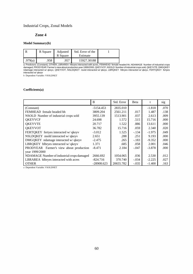
60
Industrial Crops, Zonal Models
Zone 4
Model Summary(b)
R R Square AdjustedR Square
Std. Error of theEstimate
1
.979(a) .958 .957 15927.30188a Predictors: (Constant), OTHER, LBRAREA hlbryes interacted with acres, FEMHEAD female headed hh, NDAMAGE Number of industrial cropsdamaged, PRODYEAR Farmer’s view about production year 1999/2000, QKEYVCF, NSOLD Number of industrial crops sold, QKEYVTE, DMGQKEYndamage interacted w/ qkeyv, QKEYVOT, NSLDQKEY nsold interacted w/ qkeyv, LBRQKEY hlbryes interacted w/ qkeyv, FERTQKEY fertyesinteracted w/ qkeyvb Dependent Variable: VSOLDNET
Coefficients(a)
B Std. Error Beta t sig
(Constant) -5154.453 2835.010 -1.818 .070FEMHEAD female headed hh 3809.204 2561.211 .017 1.487 .138NSOLD Number of industrial crops sold 3955.139 1513.901 .037 2.613 .009QKEYVCF 24.698 1.572 .515 15.716 .000QKEYVTE 20.717 1.522 .886 13.611 .000QKEYVOT 36.782 15.716 .059 2.340 .020FERTQKEY fertyes interacted w/ qkeyv -3.012 1.525 -.134 -1.975 .049NSLDQKEY nsold interacted w/ qkeyv 2.651 .288 .251 9.193 .000DMGQKEY ndamage interacted w/ qkeyv -2.475 .265 -.183 -9.352 .000LBRQKEY hlbryes interacted w/ qkeyv 1.371 .685 .058 2.001 .046PRODYEAR Farmer’s view about productionyear 1999/2000
-8.471 2.184 -.047 -3.878 .000
NDAMAGE Number of industrial crops damaged 2666.692 1054.065 .036 2.530 .012LBRAREA hlbryes interacted with acres -824.716 370.740 -.034 -2.225 .027OTHER -28908.623 20655.782 -.035 -1.400 .163
a Dependent Variable: VSOLDNET

61
F. Livestock, Zonal Models
Zone 1
Model Summary(b)
R R Square AdjustedR Square
Std. Error ofthe Estimate
1
.820(a) .673 .652 15807.06224a Predictors: (Constant), INT_GCOW, NCHICK, SOLDCBUL, SOLDHNY, SOLDMK, SOLDHIDE, NCCALF, NSOLD_LV, NLBULL, NSHEEP,NGCALF, NPROD_LP, NGOATb Dependent Variable: VNET_LV Net value livestock income
Coefficients(a)
B Std. Error Beta t sig
(Constant) -8408.781 3065.337 -2.743 .007NPROD_LP 7810.978 2176.520 .231 3.589 .000NLBULL -2504.211 910.495 -.160 -2.750 .006NGCALF 39384.281 8062.408 .300 4.885 .000NCCALF 5514.014 2460.414 .104 2.241 .026NSHEEP 620.888 457.080 .099 1.358 .176NGOAT 244.475 99.120 .220 2.466 .014NCHICK 302.438 90.919 .207 3.326 .001NSOLD_LV 5922.187 1751.136 .164 3.382 .001SOLDCBUL 26444.517 10280.936 .116 2.572 .011SOLDMK 10043.205 2918.763 .174 3.441 .001SOLDHNY -8364.227 5241.071 -.072 -1.596 .112SOLDHIDE -8659.147 4172.113 -.111 -2.075 .039INT_GCOW 12751.882 5182.232 .158 2.461 .015
a Dependent Variable: VNET_LV Net value livestock income

62
Livestock, Zonal Models
Zone 2
Model Summary(b)
R R Square AdjustedR Square
Std. Error of theEstimate
1
.730(a) .533 .508 14840.50375a Predictors: (Constant), INT_GCOW, SOLDCBUL, NCHICK, NLCALF, NDUCK, FEMHEAD female headed hh, NSOLD_LV, SOLDGBUL,SCH_HEAD years of schooling for hh head, SOLDGCOW, NLCOW, NGBULL, NGCOWb Dependent Variable: VNET_LV Net value livestock income
Coefficients(a)
B Std. Error Beta t sig
(Constant) 4208.773 2154.558 1.953 .052SCH_HEAD years of schooling for hh head -567.905 237.306 -.118 -2.393 .017FEMHEAD female headed hh -4416.253 2645.914 -.080 -1.669 .096NGCOW -12693.225 6792.222 -.203 -1.869 .063NLCOW 1288.536 544.300 .127 2.367 .019NGBULL -136651.321 24739.047 -.571 -5.524 .000NLCALF 3118.284 819.701 .197 3.804 .000NCHICK 191.131 99.822 .087 1.915 .057NDUCK 1856.674 865.183 .097 2.146 .033NSOLD_LV 9492.291 1293.257 .344 7.340 .000SOLDGCOW 117095.668 15126.095 .489 7.741 .000SOLDGBUL 75219.940 26238.753 .223 2.867 .005SOLDCBUL 66724.976 15294.133 .198 4.363 .000INT_GCOW 38677.162 8087.913 .566 4.782 .000
a Dependent Variable: VNET_LV Net value livestock income
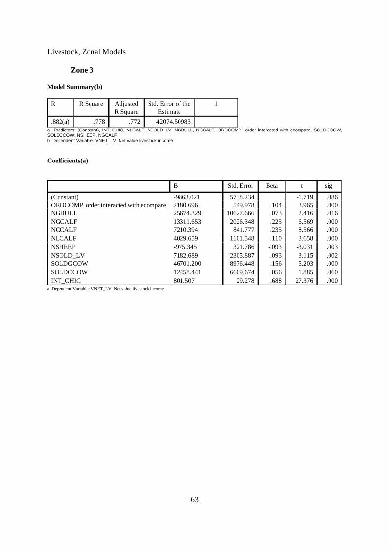
63
Livestock, Zonal Models
Zone 3
Model Summary(b)
R R Square AdjustedR Square
Std. Error of theEstimate
1
.882(a) .778 .772 42074.50983a Predictors: (Constant), INT_CHIC, NLCALF, NSOLD_LV, NGBULL, NCCALF, ORDCOMP order interacted with ecompare, SOLDGCOW,SOLDCCOW, NSHEEP, NGCALFb Dependent Variable: VNET_LV Net value livestock income
Coefficients(a)
B Std. Error Beta t sig
(Constant) -9863.021 5738.234 -1.719 .086ORDCOMP order interacted with ecompare 2180.696 549.978 .104 3.965 .000NGBULL 25674.329 10627.666 .073 2.416 .016NGCALF 13311.653 2026.348 .225 6.569 .000NCCALF 7210.394 841.777 .235 8.566 .000NLCALF 4029.659 1101.548 .110 3.658 .000NSHEEP -975.345 321.786 -.093 -3.031 .003NSOLD_LV 7182.689 2305.887 .093 3.115 .002SOLDGCOW 46701.200 8976.448 .156 5.203 .000SOLDCCOW 12458.441 6609.674 .056 1.885 .060INT_CHIC 801.507 29.278 .688 27.376 .000
a Dependent Variable: VNET_LV Net value livestock income

64
Livestock, Zonal Models
Zone 4
Model Summary(b)
R R Square AdjustedR Square
Std. Error of theEstimate
1
.561(a) .314 .293 31824.57607a Predictors: (Constant), INT_GCOW, SOLDHNY, NDUCK, NSOLD_LV, SCH_HEAD years of schooling for hh head, NADULT # of adults in hh,NSHEEP, ORDCOMP order interacted with ecompare, NPROD_LP, NCCOWb Dependent Variable: VNET_LV Net value livestock income
Coefficients(a)
B Std. Error Beta t sig
(Constant) -18886.147 8351.036 -2.262 .024NADULT # of adults in hh 1472.576 669.990 .107 2.198 .029ORDCOMP order interacted with ecompare 437.315 471.359 .045 .928 .354SCH_HEAD years of schooling for hh head 662.908 425.818 .074 1.557 .121NPROD_LP 7249.375 3639.473 .102 1.992 .047NCCOW 6429.993 2541.349 .135 2.530 .012NSHEEP -2261.054 1762.017 -.061 -1.283 .200NDUCK -7232.689 4137.208 -.083 -1.748 .081NSOLD_LV 7301.838 2125.522 .167 3.435 .001SOLDHNY 27778.957 19399.561 .070 1.432 .153INT_GCOW 17475.269 2099.111 .467 8.325 .000
a Dependent Variable: VNET_LV Net value livestock income

65
G. Informal Off-Farm, Zonal Models
Zone 1
Model Summary(b)
R R Square AdjustedR Square
Std. Error of theEstimate
1
.741(a) .550 .526 44815.07640a Predictors: (Constant), MTHBIKE, MTHTIMB, MINE mining business, DRIVER driver, MTHFSH, PVASST02 Unstandardized Predicted Value,NADULT # of adults in hh, NMTHS # of months hh had income from informal activities, TRANS transport business, ORDCOMP order interactedwith cash incomeb Dependent Variable: VINFORM earnings from all informal off-farm activities
Coefficients(a)
B Std. Error Beta t sig
(Constant) -31251.101 12372.036 -2.526 .012PVASST02 Unstandardized Predicted Value .049 .014 .171 3.397 .001ORDCOMP order interacted with cash income 1600.059 1088.766 .077 1.470 .143NMTHS # of months hh had income frominformal activities
3111.325 862.127 .186 3.609 .000
MTHTIMB 32025.551 3780.894 .420 8.470 .000DRIVER driver 138859.886 23353.210 .301 5.946 .000MINE mining business 166730.120 32437.709 .257 5.140 .000MTHFSH 4313.994 1202.770 .187 3.587 .000NADULT # of adults in hh 2611.437 1162.089 .116 2.247 .026TRANS transport business -42714.775 21314.524 -.103 -2.004 .047MTHBIKE 5332.797 2707.408 .097 1.970 .050
a Dependent Variable: VINFORM earnings from all informal off-farm activities

66
Informal Off-Farm, Zonal Models
Zone 2
Model Summary(b)
R R Square AdjustedR Square
Std. Error of theEstimate
1
.803(a) .645 .624 33754.08641a Predictors: (Constant), MTHTIMB, MTHTRANS, HAWK hawking, MTHCARP, SCH_HEAD years of schooling for hh head, RENT rental business,NADULT # of adults in hh, WAGERATE Daily wagerate, NPEOPLE # of people earning informal income, PVASST02 Unstandardized PredictedValue, MTHJAGGb Dependent Variable: VINFORM earnings from all informal off-farm activities
Coefficients(a)
B Std. Error Beta t sig
(Constant) -6967.077 12491.965 -.558 .578SCH_HEAD years of schooling for hh head 824.366 571.518 .066 1.442 .151PVASST02 Unstandardized Predicted Value .154 .033 .235 4.594 .000NADULT # of adults in hh 1818.775 919.691 .096 1.978 .049WAGERATE Daily wagerate -281.071 162.421 -.080 -1.731 .085NPEOPLE # of people earning informalincome
12749.328 5304.512 .113 2.403 .017
MTHJAGG 9809.908 2066.884 .261 4.746 .000MTHTRANS 25402.716 3580.051 .393 7.096 .000HAWK hawking 64008.656 16306.853 .183 3.925 .000RENT rental business 40678.896 11114.726 .169 3.660 .000MTHCARP 1959.687 1076.295 .082 1.821 .070MTHTIMB 2533.120 1661.087 .067 1.525 .129
a Dependent Variable: VINFORM earnings from all informal off-farm activities

67
Informal Off-Farm, Zonal Models
Zone 3
Model Summary(b)
R R Square AdjustedR Square
Std. Error of theEstimate
1
.507(a) .257 .228 91678.54995a Predictors: (Constant), MTHBREW, NPEOPLE # of people earning informal income, RENT rental business, NMTHS # of months hh had incomefrom informal activities, PVASST02 Unstandardized Predicted Value, ORDCOMP order interacted with cash income, FKIB farm kibarua, NPPLSQb Dependent Variable: VINFORM earnings from all informal off-farm activities
Coefficients(a)
B Std. Error Beta t sig
(Constant) -123839.918 34049.985 -3.637 .000ORDCOMP order interacted with cash income 7780.774 2112.632 .249 3.683 .000PVASST02 Unstandardized Predicted Value .110 .032 .223 3.388 .001FKIB farm kibarua -43053.826 17759.421 -.182 -2.424 .016NMTHS # of months hh had income frominformal activities
4797.670 1864.602 .161 2.573 .011
RENT rental business -25560.470 17710.623 -.089 -1.443 .150NPEOPLE # of people earning informalincome
74421.658 33175.035 .554 2.243 .026
NPPLSQ -10432.572 6789.869 -.366 -1.536 .126MTHBREW -5329.107 3499.001 -.092 -1.523 .129
a Dependent Variable: VINFORM earnings from all informal off-farm activities

68
Informal Off-Farm, Zonal Models
Zone 4
Model Summary(b)
R R Square AdjustedR Square
Std. Error of theEstimate
1
.704(a) .496 .464 80871.92539a Predictors: (Constant), MTHFKIB, MTHTIMB, MTHRENT, WAGERATE Daily wagerate, MTHAGTRD, SCH_HEAD years of schooling for hh head,ORDCOMP order interacted with cash income, NMTHS # of months hh had income from informal activities, NPEOPLE # of people earning informalincome, PVASST02 Unstandardized Predicted Value, RENT rental businessb Dependent Variable: VINFORM earnings from all informal off-farm activities
Coefficients(a)
B Std. Error Beta t sig
(Constant) -109004.904 28468.493 -3.829 .000SCH_HEAD years of schooling for hh head -1944.457 1532.916 -.073 -1.268 .206PVASST02 Unstandardized Predicted Value .175 .035 .314 4.995 .000ORDCOMP order interacted with cash income 7455.339 1966.758 .235 3.791 .000NMTHS # of months hh had income frominformal activities
3183.883 1656.226 .115 1.922 .056
NPEOPLE # of people earning informal income 13809.235 11423.637 .073 1.209 .228WAGERATE Daily wagerate 506.540 230.467 .123 2.198 .029MTHTIMB 26297.069 3802.570 .397 6.916 .000MTHAGTRD 3577.827 1606.443 .124 2.227 .027RENT rental business -636606.227 400687.33
2-1.160 -1.589 .114
MTHRENT 51922.461 35032.231 1.079 1.482 .140MTHFKIB -1071.322 1469.015 -.046 -.729 .467
a Dependent Variable: VINFORM earnings from all informal off-farm activities

69
H. Salaries and Remittances, Zonal Models
Zone 1
Model Summary(b)
R R Square AdjustedR Square
Std. Error of theEstimate
1
.798(a) .637 .606 41036.11433a Predictors: (Constant), MTHWATCH, SCH_HEAD years of schooling for hh head, MTHSHOP, MTHPOL, MTHCLERK, MTHDRIVE, MTHMGR,MTHREMIT, MTHSALES, MTHTEACH, MTHPENS, ORDCOMP order interacted with ecompare, NPEOPLE # of people earning sal or remit, NMTHS# of months hh had income from sal or remitb Dependent Variable: VSALREM earnings from all salary and remittance
Coefficients(a)
B Std. Error Beta t sig
(Constant) -69688.232 12345.862 -5.645 .000NPEOPLE # of people earning sal or remit 6481.401 5342.638 .071 1.213 .227NMTHS # of months hh had income from salor remit
2910.438 1094.872 .167 2.658 .009
SCH_HEAD years of schooling for hh head 2664.169 756.453 .181 3.522 .001ORDCOMP order interacted with ecompare 5255.166 902.478 .320 5.823 .000MTHREMIT -677.167 826.791 -.056 -.819 .414MTHTEACH 5141.314 994.561 .286 5.169 .000MTHDRIVE 4489.422 1257.727 .182 3.569 .000MTHMGR 10769.605 2078.873 .256 5.181 .000MTHPENS -1340.316 1305.395 -.054 -1.027 .306MTHCLERK 3630.966 1902.485 .096 1.909 .058MTHSALES 4357.810 1979.906 .108 2.201 .029MTHPOL 2271.659 2026.528 .054 1.121 .264MTHSHOP 2928.393 1967.799 .080 1.488 .139MTHWATCH -1778.914 1729.866 -.052 -1.028 .305
a Dependent Variable: VSALREM earnings from all salary and remittance

70
Salaries and Remittances, Zonal Models
Zone 2
Model Summary(b)
R R Square AdjustedR Square
Std. Error of theEstimate
1
.704(a) .496 .468 43692.46523a Predictors: (Constant), MTHCLERK, NPEOPLE # of people earning sal or remit, MTHTEACH, MTHMGR, MTHPENS, PVASST02 UnstandardizedPredicted Value, NMTHS # of months hh had income from sal or remit, SCH_HEAD years of schooling for hh head, ORDCOMP order interactedwith ecompareb Dependent Variable: VSALREM earnings from all salary and remittance
Coefficients(a)
B Std. Error Beta t sig
(Constant) -58186.314 12038.151 -4.833 .000NPEOPLE # of people earning sal or remit 33522.178 5391.670 .360 6.217 .000NMTHS # of months hh had income from salor remit
1667.729 938.769 .113 1.777 .078
PVASST02 Unstandardized Predicted Value .040 .037 .066 1.086 .279SCH_HEAD years of schooling for hh head 2065.134 859.876 .156 2.402 .017ORDCOMP order interacted with ecompare 1366.761 963.926 .093 1.418 .158MTHTEACH 3095.462 948.965 .207 3.262 .001MTHMGR 3616.480 2186.160 .095 1.654 .100MTHPENS 2329.378 1318.657 .104 1.766 .079MTHCLERK 3667.307 1330.336 .163 2.757 .007
a Dependent Variable: VSALREM earnings from all salary and remittance

71
Salaries and Remittances, Zonal Models
Zone 3\Model Summary(b)
R R Square AdjustedR Square
Std. Error of theEstimate
1
.829(a) .687 .665 49809.98011a Predictors: (Constant), MTHLEC, MTHMGR, MTHBANK, MTHPOL, MTHFARM, FEMHEAD female headed hh, MTHPENS, MTHREMIT,NPEOPLE # of people earning sal or remit, WAGERATE Daily wagerate, NMTHS # of months hh had income from sal or remit, SCH_HEAD yearsof schooling for hh head, ORDCINC order interacted with cash incomeb Dependent Variable: VSALREM earnings from all salary and remittance
Coefficients(a)
B Std. Error Beta t sig
(Constant) -123480.233 18879.941 -6.540 .000NPEOPLE # of people earning sal or remit 67491.693 7904.948 .453 8.538 .000NMTHS # of months hh had income from salor remit
4851.124 1063.831 .208 4.560 .000
WAGERATE Daily wagerate 238.792 196.004 .053 1.218 .225SCH_HEAD years of schooling for hh head 4142.078 877.734 .241 4.719 .000FEMHEAD female headed hh 18409.472 11461.247 .070 1.606 .110ORDCINC order interacted with cash income .018 .007 .138 2.476 .014MTHREMIT -2782.777 856.121 -.154 -3.250 .001MTHMGR 15439.852 2450.477 .263 6.301 .000MTHPENS -3736.420 1452.916 -.109 -2.572 .011MTHPOL 2773.551 2169.673 .054 1.278 .203MTHFARM -5072.211 1707.774 -.125 -2.970 .003MTHBANK 9461.554 2231.993 .186 4.239 .000MTHLEC 16238.312 3045.265 .226 5.332 .000
a Dependent Variable: VSALREM earnings from all salary and remittance

72
Salaries and Remittances, Zonal Models
Zone 4
Model Summary(b)
R R Square AdjustedR Square
Std. Error ofthe Estimate
1
.877(a) .768 .748 32494.49230a Predictors: (Constant), MTHCHIEF, PVASST02 Unstandardized Predicted Value, MTHPOL, MTHSALES, MTHLEC, MTHDRIVE, MTHCLERK,MTHIND, FEMHEAD female headed hh, MTHCIVIL, MTHWATCH, NPEOPLE # of people earning sal or remit, NMTHS # of months hh had incomefrom sal or remit, NADULT # of adults in hh, MTHTEACH, MTHREMIT, SCH_HEAD years of schooling for hh head, ORDCINC order interactedwith cash incomeb Dependent Variable: VSALREM earnings from all salary and remittance
Coefficients(a)
B Std. Error Beta t sig
(Constant) -60008.131 10422.249 -5.758 .000NPEOPLE # of people earning sal or remit 44281.602 5198.729 .338 8.518 .000NMTHS # of months hh had income from sal orremit
1781.927 756.740 .090 2.355 .019
PVASST02 Unstandardized Predicted Value .045 .015 .130 3.073 .002NADULT # of adults in hh -1153.658 843.397 -.050 -1.368 .173SCH_HEAD years of schooling for hh head 2156.102 644.955 .145 3.343 .001FEMHEAD female headed hh 27491.738 6337.751 .154 4.338 .000ORDCINC order interacted with cash income .005 .006 .047 .926 .355MTHREMIT -1337.522 495.348 -.116 -2.700 .008MTHTEACH 4198.708 681.652 .275 6.160 .000MTHDRIVE 6945.916 853.261 .300 8.140 .000MTHIND 3540.477 1012.836 .122 3.496 .001MTHCLERK 4350.047 822.591 .195 5.288 .000MTHSALES 5806.857 2445.994 .082 2.374 .019MTHPOL 7548.091 1969.559 .131 3.832 .000MTHWATCH 1645.652 928.100 .063 1.773 .078MTHCIVIL 5656.192 1631.649 .120 3.467 .001MTHLEC 17056.082 2793.007 .210 6.107 .000MTHCHIEF 8700.752 1281.186 .238 6.791 .000
a Dependent Variable: VSALREM earnings from all salary and remittance

73
CONDITIONAL MODELS
A. Retained Cereals and Tubers, Conditional Models
Per Capita Income Quintile 1
Model Summary
R R Square AdjustedR Square
Std. Error of theEstimate
1
.847(a) .718 .697 3870.36598a Predictors: (Constant), PRODYR3, ZEROQRET nzerohrv interacted w/ qkeyret, STPOTRET, ARROWRET, SCH_HEAD years of schooling for hh head,QKEYRGRM qkeyret interacted with green maize, QKEYRSO qkeyret interacted with sorghum, HHSIZE hh size, PVASSET3, QKEYRRI qkeyret interactedwith rice, QKEYRGRG qkeyret interacted with greengrams, ORDCOMP order interacted with ecompare, NDAMAGE number of ctp damaged, FEMHEAD2,HLBRYES2, NCTPQRET nctp interacted w/ qkeyret, PRODYR2, TACRES3, TACRES2
Coefficients(a)
B Std. Error Beta t sig
(Constant) 1107.181 939.679 1.178 .240NCTPQRET nctp interacted w/ qkeyret 1.853 .104 .803 17.778 .000QKEYRRI qkeyret interacted with rice -5.523 1.723 -.119 -3.204 .002QKEYRGRM qkeyret interacted with greenmaize
4.193 2.491 .061 1.683 .094
QKEYRGRG qkeyret interacted withgreengrams
9.572 3.286 .103 2.913 .004
QKEYRSO qkeyret interacted with sorghum 5.920 3.289 .064 1.800 .073STPOTRET -1433.536 608.864 -.083 -2.354 .019ARROWRET -13267.030 4046.180 -.115 -3.279 .001ZEROQRET nzerohrv interacted w/ qkeyret -.344 .088 -.159 -3.905 .000NDAMAGE number of ctp damaged -247.766 80.148 -.118 -3.091 .002HHSIZE hh size 333.393 70.542 .176 4.726 .000FEMHEAD2 -1544.608 785.798 -.079 -1.966 .050ORDCOMP order interacted with ecompare 150.702 72.840 .078 2.069 .040PVASSET3 -.011 .004 -.120 -2.737 .007SCH_HEAD years of schooling for hh head -123.793 66.962 -.065 -1.849 .066HLBRYES2 -3359.027 751.163 -.184 -4.472 .000TACRES2 -450.735 185.704 -.120 -2.427 .016TACRES3 -648.578 228.837 -.137 -2.834 .005PRODYR2 879.316 319.692 .131 2.751 .006PRODYR3 2.206 1.491 .053 1.480 .140
a Dependent Variable: VRETCTP

74
Retained Cereals and Tubers, Conditional Models
Per Capita Income Quintile 2
Model Summary
R R Square AdjustedR Square
Std. Error of theEstimate
1
.737(a) .544 .515 6422.47658a Predictors: (Constant), FERTAREA fertyes interacted w/ tacres, QKEYRRI qkeyret interacted with rice, QKEYRARR qkeyret interacted with arrowroots,IRPOTRET, FEMHEAD1, NSOLD2, NSOLD1, QKEYRET quant of prodn of key retained crop based on quantity retained approach, FERTYES1, NZEROHRV# of crops w/ failed harvest, FEMHEAD female headed hh, NDAMAGE number of ctp damaged, TACRES3, NCTP number of ctp produced, LBRQRET hlbryesinteracted w/ qkeyret, FERTQRET fertyes interacted w/ qkeyret
Coefficients(a)
B Std. Error Beta t sig
(Constant) 2165.438 1080.254 2.005 .046QKEYRET quant of prodn of key retained cropbased on quantity retained approach
11.742 1.011 1.388 11.620 .000
QKEYRARR qkeyret interacted with arrowroots 9.846 3.206 .131 3.071 .002QKEYRRI qkeyret interacted with rice -5.022 1.993 -.112 -2.520 .012NCTP number of ctp produced 978.717 150.730 .436 6.493 .000NDAMAGE number of ctp damaged -718.582 145.895 -.332 -4.925 .000NZEROHRV # of crops w/ failed harvest -213.251 153.815 -.068 -1.386 .167LBRQRET hlbryes interacted w/ qkeyret -2.651 .707 -.311 -3.751 .000FERTQRET fertyes interacted w/ qkeyret -5.432 .989 -.663 -5.492 .000FEMHEAD female headed hh -2113.191 1346.505 -.079 -1.569 .118FEMHEAD1 4096.988 2561.587 .084 1.599 .111TACRES3 -234.330 153.602 -.098 -1.526 .128NSOLD1 1497.717 446.862 .163 3.352 .001NSOLD2 -830.170 340.769 -.111 -2.436 .016FERTYES1 -7792.997 2269.495 -.159 -3.434 .001IRPOTRET -3161.820 1865.741 -.073 -1.695 .091FERTAREA fertyes interacted w/ tacres 259.330 122.329 .134 2.120 .035
a Dependent Variable: VRETCTP

75
Retained Cereals and Tubers, Conditional Models
Per Capita Income Quintile 3
Model Summary
R R Square AdjustedR Square
Std. Error of theEstimate
1
.794(a) .631 .606 7254.91856a Predictors: (Constant), STPOTRET, NCTPQRET nctp interacted w/ qkeyret, FEMHEAD3, NDAMAGE2, NZEROHRV # of crops w/ failed harvest,NDAMAGE3, FEMHEAD2, TACRES1, QKEYRIP qkeyret interacted with irishpotatoes, NCTP number of ctp produced, TACRES2, QKEYRSTP qkeyretinteracted with sweetpotatoes, NDAMAGE1, LBRQRET hlbryes interacted w/ qkeyret, NSLDQRET nsold interacted w/ qkeyret, FERTQRET fertyes interactedw/ qkeyret, QKEYRET quant of prodn of key retained crop based on quantity retained approach
Coefficients(a)
B Std. Error Beta t sig
(Constant) -203.055 1467.991 -.138 .890NCTPQRET nctp interacted w/ qkeyret .357 .148 .311 2.419 .016NCTP number of ctp produced 924.006 172.438 .327 5.358 .000QKEYRET quant of prodn of key retained cropbased on quantity retained approach
10.284 1.372 1.379 7.496 .000
QKEYRIP qkeyret interacted with irishpotatoes -3.070 .584 -.236 -5.255 .000QKEYRSTP qkeyret interacted withsweetpotatoes
5.840 1.661 .191 3.517 .001
NDAMAGE1 -471.003 230.031 -.136 -2.048 .042NDAMAGE2 -1479.663 309.362 -.242 -4.783 .000NDAMAGE3 -433.646 279.976 -.065 -1.549 .123NZEROHRV # of crops w/ failed harvest -319.884 127.768 -.104 -2.504 .013NSLDQRET nsold interacted w/ qkeyret -.722 .173 -.359 -4.174 .000FERTQRET fertyes interacted w/ qkeyret -3.660 .892 -.496 -4.105 .000LBRQRET hlbryes interacted w/ qkeyret -2.369 .721 -.325 -3.285 .001TACRES2 1132.241 195.933 .313 5.779 .000FEMHEAD2 -5837.639 3124.497 -.080 -1.868 .063FEMHEAD3 6978.404 2863.666 .096 2.437 .016TACRES1 463.801 220.088 .134 2.107 .036STPOTRET -3436.711 2118.583 -.086 -1.622 .106
a Dependent Variable: VRETCTP

76
Retained Cereals and Tubers, Conditional Models
Per Capita Income Quintile 4
Model Summary
R R Square AdjustedR Square
Std. Error of theEstimate
1
.938(a) .881 .871 11926.94056a Predictors: (Constant), YAMSRET, LBRQRET hlbryes interacted w/ qkeyret, NZERO1, QKEYRSTP qkeyret interacted with sweetpotatoes, QKEYRWHqkeyret interacted with wheat, PVASSET2, ORDCOMP order interacted with ecompare, FERTYES Used fertilizer, NCTP number of ctp produced, NSOLD3,HLBRYES used hired labour, HLBRYES1, QKEYRYA qkeyret interacted with yams, NDAMAGE3, TACRES2, SCHHEAD3, FERTQRET fertyes interactedw/ qkeyret, TACRES1, NCTPQRET nctp interacted w/ qkeyret, NSLDQRET nsold interacted w/ qkeyret, QKEYRET quant of prodn of key retained crop basedon quantity retained approach
Coefficients(a)
B Std. Error Beta t sig
(Constant) -12531.813 4004.458 -3.129 .002NCTPQRET nctp interacted w/ qkeyret .464 .134 .263 3.466 .001NCTP number of ctp produced 759.393 269.015 .087 2.823 .005QKEYRET quant of prodn of key retained cropbased on quantity retained approach
21.120 1.408 1.683 15.001 .000
QKEYRYA qkeyret interacted with yams 14.414 2.375 .192 6.069 .000QKEYRWH qkeyret interacted with wheat 4.125 1.900 .050 2.171 .031QKEYRSTP qkeyret interacted withsweetpotatoes
-4.154 1.620 -.066 -2.564 .011
NDAMAGE3 -1158.530 597.862 -.060 -1.938 .054NZERO1 -412.516 223.380 -.044 -1.847 .066FERTQRET fertyes interacted w/ qkeyret -12.765 .781 -.879 -16.336 .000LBRQRET hlbryes interacted w/ qkeyret -5.285 .823 -.414 -6.423 .000NSLDQRET nsold interacted w/ qkeyret -1.276 .237 -.314 -5.381 .000ORDCOMP order interacted with ecompare 303.977 203.630 .035 1.493 .137SCHHEAD3 -588.410 245.135 -.078 -2.400 .017TACRES2 659.739 414.126 .048 1.593 .112PVASSET2 -.019 .014 -.040 -1.373 .171TACRES1 1397.266 302.214 .192 4.623 .000FERTYES Used fertilizer 10858.974 2085.146 .141 5.208 .000HLBRYES1 -14043.108 4373.504 -.111 -3.211 .001NSOLD3 3073.141 746.734 .134 4.115 .000HLBRYES used hired labour 3824.161 2006.895 .058 1.906 .058YAMSRET -17159.120 5921.688 -.082 -2.898 .004
a Dependent Variable: VRETCTP

77
Retained Cereals and Tubers, Conditional Models
Per Capita Income Quintile 5
Model Summary
R R Square AdjustedR Square
Std. Error of theEstimate
1
.900(a) .810 .795 13009.44416a Predictors: (Constant), FERTYES3, QKEYRPIP qkeyret interacted with pigeon peas, QKEYRCOW qkeyret interacted with cowpeas, QKEYRSTP qkeyretinteracted with sweetpotatoes, NSOLD number of ctp sold, PRODYR3, ORDCOMP order interacted with ecompare, QKEYRIP qkeyret interacted withirishpotatoes, FERTYES Used fertilizer, TACRES1, DMGQRET ndamage interacted w/ qkeyret, LBRQRET hlbryes interacted w/ qkeyret, NSOLD1,NDAMAGE3, NSOLD3, ZEROQRET nzerohrv interacted w/ qkeyret, NSLDQRET nsold interacted w/ qkeyret, QKEYRET quant of prodn of key retained cropbased on quantity retained approach, NCTPQRET nctp interacted w/ qkeyret
Coefficients(a)
B Std. Error Beta t sig
(Constant) 2222.803 3584.807 .620 .536NCTPQRET nctp interacted w/ qkeyret .378 .102 .532 3.719 .000QKEYRET quant of prodn of key retained cropbased on quantity retained approach
3.224 .653 .634 4.938 .000
QKEYRPIP qkeyret interacted with pigeon peas 13.376 1.178 .349 11.357 .000QKEYRCOW qkeyret interacted with cowpeas 27.514 3.855 .395 7.137 .000QKEYRSTP qkeyret interacted with sweetpotatoes 4.682 .532 .454 8.796 .000QKEYRIP qkeyret interacted with irishpotatoes -2.721 .645 -.171 -4.217 .000ZEROQRET nzerohrv interacted w/ qkeyret -.872 .310 -.238 -2.810 .005PRODYR3 8.122 4.081 .062 1.990 .048NDAMAGE3 -1845.813 740.278 -.109 -2.493 .013LBRQRET hlbryes interacted w/ qkeyret -1.780 .387 -.338 -4.594 .000NSLDQRET nsold interacted w/ qkeyret -.545 .143 -.469 -3.812 .000DMGQRET ndamage interacted w/ qkeyret .223 .074 .145 3.007 .003ORDCOMP order interacted with ecompare 387.871 235.220 .050 1.649 .100TACRES1 352.758 179.058 .082 1.970 .050NSOLD number of ctp sold 1250.989 535.145 .103 2.338 .020NSOLD1 -2151.921 884.972 -.108 -2.432 .016NSOLD3 1498.252 820.180 .096 1.827 .069FERTYES Used fertilizer 4495.063 2780.637 .054 1.617 .107FERTYES3 -6598.913 3301.621 -.108 -1.999 .047
a Dependent Variable: VRETCTP
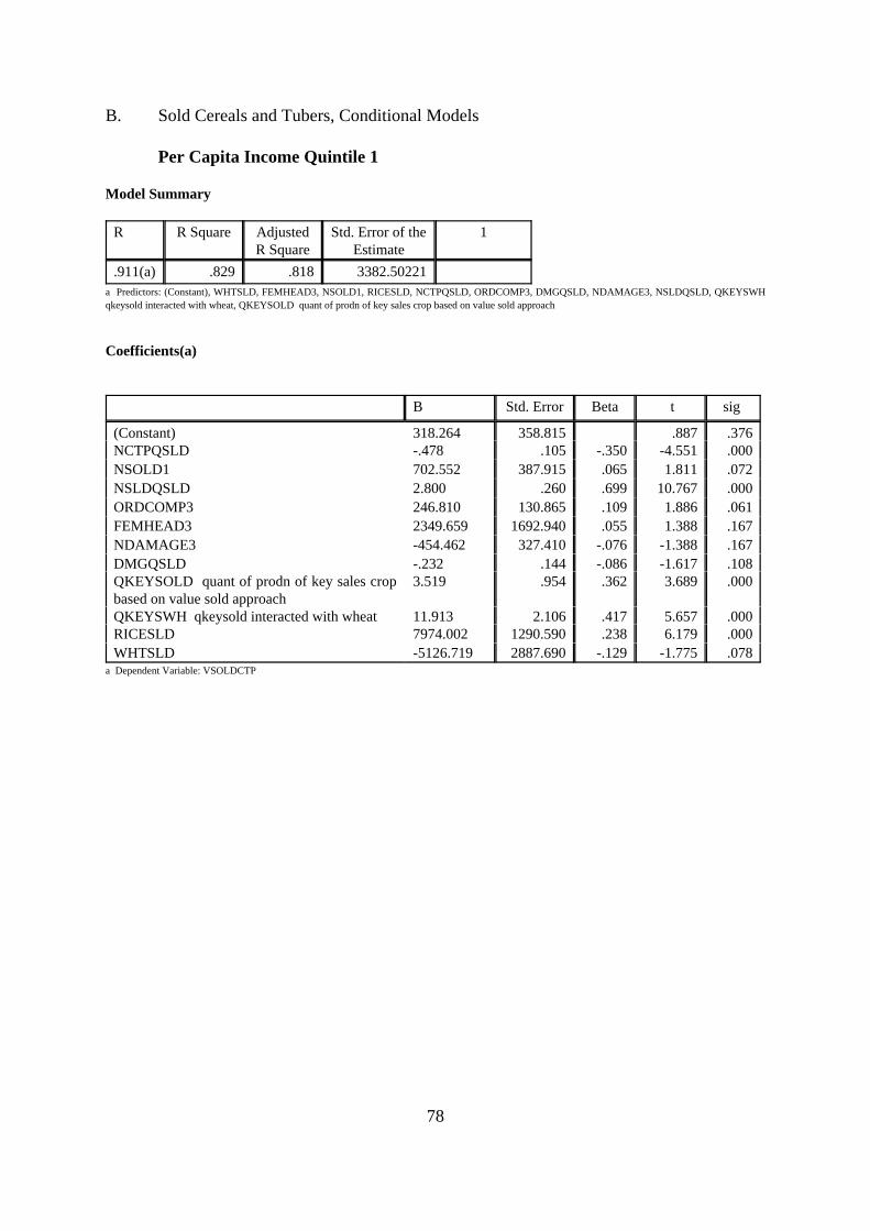
78
B. Sold Cereals and Tubers, Conditional Models
Per Capita Income Quintile 1
Model Summary
R R Square AdjustedR Square
Std. Error of theEstimate
1
.911(a) .829 .818 3382.50221a Predictors: (Constant), WHTSLD, FEMHEAD3, NSOLD1, RICESLD, NCTPQSLD, ORDCOMP3, DMGQSLD, NDAMAGE3, NSLDQSLD, QKEYSWHqkeysold interacted with wheat, QKEYSOLD quant of prodn of key sales crop based on value sold approach
Coefficients(a)
B Std. Error Beta t sig
(Constant) 318.264 358.815 .887 .376NCTPQSLD -.478 .105 -.350 -4.551 .000NSOLD1 702.552 387.915 .065 1.811 .072NSLDQSLD 2.800 .260 .699 10.767 .000ORDCOMP3 246.810 130.865 .109 1.886 .061FEMHEAD3 2349.659 1692.940 .055 1.388 .167NDAMAGE3 -454.462 327.410 -.076 -1.388 .167DMGQSLD -.232 .144 -.086 -1.617 .108QKEYSOLD quant of prodn of key sales cropbased on value sold approach
3.519 .954 .362 3.689 .000
QKEYSWH qkeysold interacted with wheat 11.913 2.106 .417 5.657 .000RICESLD 7974.002 1290.590 .238 6.179 .000WHTSLD -5126.719 2887.690 -.129 -1.775 .078
a Dependent Variable: VSOLDCTP

79
Sold Cereals and Tubers, Conditional Models
Per Capita Income Quintile 2
Model Summary
R R Square AdjustedR Square
Std. Error of theEstimate
1
.912(a) .832 .824 5503.70591a Predictors: (Constant), QKEYSRI qkeysold interacted with rice, QKEYSWH qkeysold interacted with wheat, PRODYEAR Farmer’s view about productionyear 1999/2000, NSOLD number of ctp sold, NCTPQSLD, LBRQSLD, NSLDQSLD, QKEYSOLD quant of prodn of key sales crop based on value sold approach
Coefficients(a)
B Std. Error Beta t sig
(Constant) -1709.209 1065.173 -1.605 .111NCTPQSLD -.155 .077 -.114 -2.003 .047NSOLD number of ctp sold 585.981 333.982 .087 1.755 .081NSLDQSLD 1.238 .226 .414 5.487 .000PRODYEAR Farmer’s view about production year1999/2000
2.304 1.429 .052 1.612 .109
LBRQSLD -1.340 .639 -.155 -2.098 .037QKEYSOLD quant of prodn of key sales cropbased on value sold approach
5.477 .908 .596 6.030 .000
QKEYSWH qkeysold interacted with wheat 5.337 .760 .242 7.026 .000QKEYSRI qkeysold interacted with rice 8.022 1.013 .275 7.920 .000
a Dependent Variable: VSOLDCTP

80
Sold Cereals and Tubers, Conditional Models
Per Capita Income Quintile 3
Model Summary
R R Square AdjustedR Square
Std. Error of theEstimate
1
.954(a) .910 .905 6874.22468a Predictors: (Constant), QKEYSSTP qkeysold interacted with sweetpotatoes, NCTPQSLD, QKEYSMI qkeysold interacted with millet, QKEYSCA qkeysoldinteracted with cassava, QKEYSWH qkeysold interacted with wheat, DMGQSLD, QKEYSOLD quant of prodn of key sales crop based on value sold approach,NSLDQSLD
Coefficients(a)
B Std. Error Beta t sig
(Constant) 325.463 708.620 .459 .647NCTPQSLD -.296 .120 -.182 -2.464 .015NSLDQSLD .998 .166 .300 6.023 .000DMGQSLD .213 .109 .074 1.954 .052QKEYSOLD quant of prodn of key sales cropbased on value sold approach
6.419 .446 .693 14.407 .000
QKEYSWH qkeysold interacted with wheat 4.847 .530 .255 9.141 .000QKEYSMI qkeysold interacted with millet 14.106 3.078 .109 4.583 .000QKEYSCA qkeysold interacted with cassava -4.790 1.458 -.088 -3.286 .001QKEYSSTP qkeysold interacted withsweetpotatoes
-3.790 1.120 -.080 -3.384 .001
a Dependent Variable: VSOLDCTP

81
Sold Cereals and Tubers, Conditional Models
Per Capita Income Quintile 4
Model Summary
R R Square AdjustedR Square
Std. Error of theEstimate
1
.886(a) .786 .774 13237.31784a Predictors: (Constant), QKEYSGNT qkeysold interacted with groundnuts, QKEYSWH qkeysold interacted with wheat, LBRQSLD, FERTYES Used fertilizer,NSOLD number of ctp sold, ORDCOMP3, TACRES total acres cultivated, FERTQSLD, QKEYSOLD quant of prodn of key sales crop based on value soldapproach
Coefficients(a)
B Std. Error Beta t sig
(Constant) -889.414 3097.167 -.287 .774NSOLD number of ctp sold 2666.759 612.548 .173 4.354 .000ORDCOMP3 384.549 185.127 .090 2.077 .039TACRES total acres cultivated 377.436 168.906 .096 2.235 .027FERTYES Used fertilizer -9584.873 3141.288 -.132 -3.051 .003FERTQSLD 7.456 .847 .710 8.803 .000LBRQSLD 2.540 .880 .269 2.888 .004QKEYSOLD quant of prodn of key sales cropbased on value sold approach
-1.922 1.134 -.199 -1.695 .092
QKEYSWH qkeysold interacted with wheat 5.476 1.345 .158 4.071 .000QKEYSGNT qkeysold interacted withgroundnuts
50.184 14.829 .129 3.384 .001
a Dependent Variable: VSOLDCTP

82
Sold Cereals and Tubers, Conditional Models
Per Capita Income Quintile 5
Model Summary
R R Square AdjustedR Square
Std. Error ofthe Estimate
1
.957(a) .916 .911 25278.51185a Predictors: (Constant), BNSSLD, SCH_HEAD years of schooling for hh head, QKEYSWH qkeysold interacted with wheat, QKEYSIP qkeysold interactedwith irish potatoes, ORDCOMP order interacted with ecompare, PVASST02 Unstandardized Predicted Value, FERTQSLD, NSLDQSLD, NCTPQSLD,QKEYSOLD quant of prodn of key sales crop based on value sold approach
Coefficients(a)
B Std. Error Beta t sig
(Constant) -8554.964 8158.553 -1.049 .296NCTPQSLD -.301 .163 -.159 -1.850 .066NSLDQSLD 1.908 .214 .660 8.923 .000ORDCOMP order interacted with ecompare 1084.746 577.025 .046 1.880 .062SCH_HEAD years of schooling for hh head -876.680 421.371 -.051 -2.081 .039PVASST02 Unstandardized Predicted Value .010 .007 .036 1.340 .182FERTQSLD -2.875 1.250 -.226 -2.301 .023QKEYSOLD quant of prodn of key sales cropbased on value sold approach
7.194 1.626 .565 4.423 .000
QKEYSWH qkeysold interacted with wheat 5.736 .701 .227 8.187 .000QKEYSIP qkeysold interacted with irishpotatoes
-2.637 .949 -.084 -2.779 .006
BNSSLD 11343.470 7490.660 .036 1.514 .132a Dependent Variable: VSOLDCTP

83
C. Retained f&v, Conditional Models
Per Capita Income Quintile 1
Model Summary
R R Square AdjustedR Square
Std. Error ofthe Estimate
1
.704(a) .496 .450 4070.45399a Predictors: (Constant), CPLVSRET, QKEYRTO qkeyret interacted w/ tomato, QKEYROR qkeyret interacted w/ orange, QKEYRCC qkeyret interacted w/coconut, ZEROQRET nzerohrv interacted w/ qkeyret, QKEYRMG qkeyret interacted w/ mango, SUKRET, NFV3, AVOCRET, NADULT # of adults in hh,PRODYEAR Farmer’s view about production year 1999/2000, NDAMAGE1, FERTYES3, ORNGRET, NADULT2, NZERO1, COCORET, NSLDQRET nsoldinteracted w/ qkeyret, NFV1, NADULT3, NFVQRET nfv interacted w/ qkeyret, QKEYRET quant of prodn of key retained crop based on quantity retainedapproach
Coefficients(a)
B Std. Error Beta t sig
(Constant) 595.810 691.944 .861 .390NFV1 404.104 166.192 .248 2.432 .016NFV3 724.563 208.082 .275 3.482 .001NFVQRET nfv interacted w/ qkeyret .462 .162 .554 2.847 .005NSLDQRET nsold interacted w/ qkeyret -.464 .136 -.343 -3.405 .001NADULT # of adults in hh 726.454 131.278 .383 5.534 .000NADULT2 -524.020 139.852 -.294 -3.747 .000NADULT3 -807.254 186.439 -.452 -4.330 .000NDAMAGE1 -970.161 239.074 -.334 -4.058 .000NZERO1 285.508 126.676 .154 2.254 .025ZEROQRET nzerohrv interacted w/ qkeyret -.368 .069 -.552 -5.370 .000PRODYEAR Farmer’s view about productionyear 1999/2000
1.363 .995 .088 1.370 .172
FERTYES3 -2384.583 1030.795 -.144 -2.313 .022QKEYRET quant of prodn of key retained cropbased on quantity retained approach
4.359 1.307 .659 3.335 .001
QKEYROR qkeyret interacted w/ orange 5.951 2.724 .141 2.184 .030QKEYRTO qkeyret interacted w/ tomato -3.713 2.010 -.095 -1.847 .066QKEYRMG qkeyret interacted w/ mango -3.987 .893 -.505 -4.465 .000QKEYRCC qkeyret interacted w/ coconut -5.724 1.569 -.292 -3.648 .000AVOCRET -1325.081 967.230 -.068 -1.370 .172COCORET -2996.455 2197.490 -.099 -1.364 .174SUKRET -1858.316 959.961 -.092 -1.936 .054ORNGRET -2804.159 1788.799 -.098 -1.568 .118CPLVSRET -1879.470 976.321 -.093 -1.925 .055
a Dependent Variable: VRETFV

84
Retained f&v, Conditional Models
Per Capita Income Quintile 2
Model Summary
R R Square AdjustedR Square
Std. Error ofthe Estimate
1
.623(a) .388 .346 5099.85909a Predictors: (Constant), GUAVARET, HLBRYES used hired labour, FEMHEAD3, QKEYRMG qkeyret interacted w/ mango, QKEYROR qkeyret interactedw/ orange, QKEYRCB qkeyret interacted w/ cabbage, PVASSET2, TACRES total cropped acres, NSOLD number of f&v sold, NDAMAGE number of f&vdamaged, FERTYES3, TACRES1, NFV number of f&v produced, HLBRYES3, TACRES3, QKEYRGV qkeyret interacted w/ guava, QKEYRET quant of prodnof key retained crop based on quantity retained approach
Coefficients(a)
B Std. Error Beta t sig
(Constant) 43.653 845.317 .052 .959NFV number of f&v produced 821.222 123.125 .422 6.670 .000NSOLD number of f&v sold -358.080 199.329 -.108 -1.796 .074PVASSET2 -.008 .006 -.070 -1.290 .198FEMHEAD3 3380.616 1526.996 .116 2.214 .028TACRES total cropped acres 163.347 87.889 .141 1.859 .064TACRES1 -337.760 127.113 -.174 -2.657 .008TACRES3 -240.567 121.826 -.157 -1.975 .049NDAMAGE number of f&v damaged -227.978 145.000 -.089 -1.572 .117FERTYES3 -1682.920 921.728 -.109 -1.826 .069HLBRYES used hired labour -4011.191 1734.334 -.147 -2.313 .022HLBRYES3 10079.743 3139.546 .218 3.211 .002QKEYRET quant of prodn of key retained cropbased on quantity retained approach
3.553 .625 .599 5.689 .000
QKEYRGV qkeyret interacted w/ guava 5.912 5.302 .097 1.115 .266QKEYRMG qkeyret interacted w/ mango -1.877 .673 -.287 -2.790 .006QKEYROR qkeyret interacted w/ orange -2.751 1.615 -.090 -1.704 .090QKEYRCB qkeyret interacted w/ cabbage -3.891 2.395 -.088 -1.624 .106GUAVARET -3386.567 2436.592 -.120 -1.390 .166
a Dependent Variable: VRETFV

85
Retained f&v, Conditional Models
Per Capita Income Quintile 3
Model Summary
R R Square AdjustedR Square
Std. Error ofthe Estimate
1
.692(a) .479 .440 7106.16639a Predictors: (Constant), COCORET, NZERO1, QKEYRTO qkeyret interacted w/ tomato, QKEYRMG qkeyret interacted w/ mango, QKEYRCB qkeyretinteracted w/ cabbage, PAPARET, NDAMAGE2, AVOCRET, FERTYES3, SUKRET, NFV number of f&v produced, LBRQRET hlbryes interacted w/ qkeyret,NDAMAGE1, PRODYR2, NZEROHRV, QKEYRET quant of prodn of key retained crop based on quantity retained approach, TACRES2, NFV2
Coefficients(a)
B Std. Error Beta t sig
(Constant) 1488.035 1241.817 1.198 .232NFV number of f&v produced 729.113 135.335 .308 5.387 .000NFV2 940.804 382.681 .265 2.458 .015TACRES2 515.502 245.997 .175 2.096 .037NDAMAGE1 -297.175 215.024 -.084 -1.382 .168NDAMAGE2 -1333.984 452.786 -.193 -2.946 .004NZEROHRV -268.949 159.151 -.102 -1.690 .092NZERO1 370.653 251.449 .094 1.474 .142PRODYR2 -2661.496 983.947 -.252 -2.705 .007FERTYES3 -2918.801 1220.145 -.120 -2.392 .018LBRQRET hlbryes interacted w/ qkeyret 1.924 1.217 .087 1.582 .115QKEYRET quant of prodn of key retained cropbased on quantity retained approach
4.257 .455 .721 9.356 .000
QKEYRMG qkeyret interacted w/ mango -3.545 .565 -.476 -6.278 .000QKEYRCB qkeyret interacted w/ cabbage -7.162 1.459 -.260 -4.908 .000QKEYRTO qkeyret interacted w/ tomato -5.478 3.387 -.080 -1.617 .107AVOCRET -2239.439 1326.861 -.087 -1.688 .093PAPARET -4553.089 2283.584 -.096 -1.994 .047SUKRET -3201.077 1323.157 -.121 -2.419 .016COCORET -6958.581 3122.404 -.118 -2.229 .027
a Dependent Variable: VRETFV

86
Retained f&v, Conditional Models
Per Capita Income Quintile 4
Model Summary
R R Square AdjustedR Square
Std. Error ofthe Estimate
1
.780(a) .609 .575 9525.45208
a Predictors: (Constant), INDIGRET, FEMHEAD female headed hh, NSLDQRET nsold interacted w/ qkeyret,NZERO3, QKEYRTO qkeyret interacted w/ tomato, QKEYRSU qkeyret interacted w/ sukuma, QKEYRCBqkeyret interacted w/ cabbage, QKEYRMG qkeyret interacted w/ mango, NSOLD2, HLBRYES1, NDAMAGE1,PVASSET2, NSOLD3, QKEYRIV qkeyret interacted w/ indigveg, ZEROQRET nzerohrv interacted w/ qkeyret,NSOLD number of f&v sold, ORDCOMP1, NADULT2, NSOLD1, QKEYRAV qkeyret interacted w/ avocado,QKEYRET quant of prodn of key retained crop based on quantity retained approach
Coefficients(a)
B Std. Error Beta t sig
(Constant) 540.867 1029.681 .525 .600NSOLD number of f&v sold 1533.186 281.207 .348 5.452 .000NSOLD1 2368.357 600.629 .334 3.943 .000NSOLD2 -1456.871 507.690 -.163 -2.870 .004NSOLD3 -1037.708 367.781 -.149 -2.822 .005NSLDQRET nsold interacted w/ qkeyret -.353 .078 -.564 -4.529 .000NADULT2 880.556 337.865 .165 2.606 .010PVASSET2 -.018 .011 -.084 -1.571 .117ORDCOMP1 -374.309 226.134 -.111 -1.655 .099FEMHEAD female headed hh 5450.096 1833.029 .122 2.973 .003NDAMAGE1 594.896 402.631 .088 1.478 .141NZERO3 509.234 297.429 .076 1.712 .088ZEROQRET nzerohrv interacted w/ qkeyret -.337 .163 -.109 -2.065 .040HLBRYES1 -11993.027 4771.943 -.132 -2.513 .013QKEYRET quant of prodn of key retained cropbased on quantity retained approach
10.316 .879 2.255 11.729 .000
QKEYRMG qkeyret interacted w/ mango -6.806 1.640 -.184 -4.149 .000QKEYRAV qkeyret interacted w/ avocado -7.341 .739 -1.553 -9.936 .000QKEYRCB qkeyret interacted w/ cabbage -7.656 1.476 -.240 -5.186 .000QKEYRTO qkeyret interacted w/ tomato -7.560 2.015 -.164 -3.752 .000QKEYRSU qkeyret interacted w/ sukuma -7.432 1.614 -.205 -4.604 .000QKEYRIV qkeyret interacted w/ indigveg 6.976 3.018 .118 2.312 .022INDIGRET -6090.858 4371.731 -.071 -1.393 .165
a Dependent Variable: VRETFV

87
Retained f&v, Conditional Models
Per Capita Income Quintile 5
Model Summary
R R Square AdjustedR Square
Std. Error ofthe Estimate
1
.849(a) .721 .699 9591.50849a Predictors: (Constant), COCORET, FEMHEAD2, FEMHEAD1, QKEYRPU qkeyret interacted w/ pumpkin, QKEYRCB qkeyret interacted w/ cabbage,FERTYES3, SCH_HEAD years of schooling for hh head, FERTQRET fertyes interacted w/ qkeyret, HLBRYES used hired labour, FERTYES1, NFV numberof f&v produced, PVASSET1, HLBRYES3, QKEYRCC qkeyret interacted w/ coconut, NDAMAGE1, NFVQRET nfv interacted w/ qkeyret, PRODYR1,ORDCOMP1, QKEYRET quant of prodn of key retained crop based on quantity retained approach
Coefficients(a)
B Std. Error Beta t sig
(Constant) -1916.317 1743.486 -1.099 .273NFV number of f&v produced 1186.232 176.170 .288 6.733 .000NFVQRET nfv interacted w/ qkeyret -.272 .058 -1.218 -4.712 .000ORDCOMP1 1659.112 392.149 .394 4.231 .000SCH_HEAD years of schooling for hh head -202.865 128.153 -.056 -1.583 .115PVASSET1 -.021 .007 -.162 -3.076 .002FEMHEAD1 -9431.980 5638.286 -.066 -1.673 .096FEMHEAD2 64929.207 9637.891 .228 6.737 .000NDAMAGE1 793.620 413.210 .106 1.921 .056PRODYR1 -10669.497 2092.989 -.454 -5.098 .000FERTYES1 10327.453 4185.811 .137 2.467 .014FERTYES3 -3316.955 1525.688 -.082 -2.174 .031FERTQRET fertyes interacted w/ qkeyret -2.449 .502 -.430 -4.876 .000HLBRYES used hired labour -2945.468 2039.397 -.062 -1.444 .150HLBRYES3 9710.898 4143.428 .101 2.344 .020QKEYRET quant of prodn of key retained cropbased on quantity retained approach
7.789 1.077 2.120 7.229 .000
QKEYRCC qkeyret interacted w/ coconut -3.082 .383 -.488 -8.046 .000QKEYRCB qkeyret interacted w/ cabbage -2.420 .584 -.160 -4.144 .000QKEYRPU qkeyret interacted w/ pumpkin 3.941 1.326 .107 2.971 .003COCORET 50715.778 9212.771 .307 5.505 .000
a Dependent Variable: VRETFV

88
D. Sold f&v, Conditional Models
Per Capita Income Quintile 1
Model Summary
R R Square AdjustedR Square
Std. Error ofthe Estimate
1
.621(a) .386 .351 4980.53571a Predictors: (Constant), QKEYSOLD quant of prodn of key sales crop based on value sold approach, NDAMAGE3, FERTYES Used fertilizer, 1 yes, 0 no,ORDCOMP order interacted with ecompare, SCH_HEAD years of schooling for hh head, NSOLD number of f&v sold, TACRES2, PVASST02 UnstandardizedPredicted Value, TACRES3, NSOLD2, NFVQSLD nfv interacted w/ qkeysold
Coefficients(a)
B Std. Error Beta t sig
(Constant) -2838.255 1052.179 -2.698 .008NSOLD number of f&v sold 2003.361 316.634 .516 6.327 .000NSOLD2 -1271.768 366.303 -.347 -3.472 .001NFVQSLD nfv interacted w/ qkeysold -.215 .120 -.253 -1.793 .075ORDCOMP order interacted with ecompare 188.717 109.392 .108 1.725 .086SCH_HEAD years of schooling for hh head -190.739 103.447 -.111 -1.844 .067PVASST02 Unstandardized Predicted Value -.013 .005 -.185 -2.786 .006TACRES2 867.497 272.474 .253 3.184 .002TACRES3 -836.717 318.339 -.198 -2.628 .009NDAMAGE3 1609.482 352.917 .340 4.561 .000FERTYES Used fertilizer, 1 yes, 0 no 1820.711 852.420 .144 2.136 .034QKEYSOLD quant of prodn of key sales cropbased on value sold approach
3.481 .948 .516 3.674 .000
a Dependent Variable: VSOLDFV

89
Sold f&v, Conditional Models
Per Capita Income Quintile 2
Model Summary
R R Square AdjustedR Square
Std. Error ofthe Estimate
1
.781(a) .609 .589 3684.05747a Predictors: (Constant), QKEYSSU qkeysold interacted w/ sukuma, PVASSET3, QKEYSAV qkeysold interacted w/ avocado, NSOLD number of f&v sold,QKEYSOLD quant of prodn of key sales crop based on value sold approach, NSOLD2, FERTYES Used fertilizer, 1 yes, 0 no, LBRQSLD hlbryes interacted w/qkeysold, NFV1, FERTQSLD fertyes interacted w/ qkeysold
Coefficients(a)
B Std. Error Beta t sig
(Constant) 973.929 591.888 1.645 .101NFV1 -212.437 80.291 -.159 -2.646 .009NSOLD number of f&v sold 1111.502 161.853 .370 6.867 .000NSOLD2 -565.841 228.207 -.139 -2.480 .014PVASSET3 -.017 .005 -.188 -3.789 .000FERTYES Used fertilizer, 1 yes, 0 no -926.470 678.582 -.081 -1.365 .174FERTQSLD fertyes interacted w/ qkeysold 6.028 .845 .716 7.131 .000LBRQSLD hlbryes interacted w/ qkeysold -2.441 .814 -.227 -2.998 .003QKEYSOLD quant of prodn of key sales cropbased on value sold approach
1.366 .278 .277 4.916 .000
QKEYSAV qkeysold interacted w/ avocado -6.026 1.009 -.347 -5.974 .000QKEYSSU qkeysold interacted w/ sukuma -3.615 1.004 -.173 -3.599 .000
a Dependent Variable: VSOLDFV

90
Sold f&v, Conditional Models
Per Capita Income Quintile 3
Model Summary
R R Square AdjustedR Square
Std. Error ofthe Estimate
1
.663(a) .440 .403 14200.10964a Predictors: (Constant), TOMSLD, NSOLD number of f&v sold, PVASST02 Unstandardized Predicted Value, SCH_HEAD years of schooling for hh head,FERTYES2, QKEYSOLD quant of prodn of key sales crop based on value sold approach, HLBRYES1, CBBGSLD, NSOLD3, DMGQSLD ndamage interactedw/ qkeysold, QKEYSCB qkeysold interacted w/ cabbage, NSLDQSLD nsold interacted w/ qkeysold, NFVQSLD nfv interacted w/ qkeysold
Coefficients(a)
B Std. Error Beta t sig
(Constant) -3232.389 2788.216 -1.159 .248NFVQSLD nfv interacted w/ qkeysold -.984 .318 -.535 -3.092 .002NSOLD number of f&v sold 2211.433 548.861 .298 4.029 .000NSOLD3 -1284.405 588.876 -.130 -2.181 .030NSLDQSLD nsold interacted w/ qkeysold 2.373 .525 .663 4.519 .000SCH_HEAD years of schooling for hh head 346.596 264.490 .075 1.310 .192PVASST02 Unstandardized Predicted Value .010 .007 .085 1.537 .126DMGQSLD ndamage interacted w/ qkeysold -.699 .318 -.187 -2.196 .029FERTYES2 -4856.936 3475.598 -.080 -1.397 .164HLBRYES1 -9080.265 5678.220 -.101 -1.599 .111QKEYSOLD quant of prodn of key sales cropbased on value sold approach
7.930 3.017 .411 2.628 .009
QKEYSCB qkeysold interacted w/ cabbage 6.037 3.866 .162 1.562 .120CBBGSLD -11988.708 6181.429 -.188 -1.939 .054TOMSLD -5571.376 3584.022 -.085 -1.555 .122
a Dependent Variable: VSOLDFV

91
Sold f&v, Conditional Models
Per Capita Income Quintile 4
Model Summary
R R Square AdjustedR Square
Std. Error ofthe Estimate
1
.725(a) .525 .501 21228.13497a Predictors: (Constant), QKEYSSU qkeysold interacted w/ sukuma, QKEYSOLD quant of prodn of key sales crop based on value sold approach, PRODYR3,ORDCOMP1, NSOLD number of f&v sold, PRODYEAR Farmer’s view about production year 1999/2000, DMGQSLD ndamage interacted w/ qkeysold,QKEYSAV qkeysold interacted w/ avocado, NFVQSLD nfv interacted w/ qkeysold, NSLDQSLD nsold interacted w/ qkeysold
Coefficients(a)
B Std. Error Beta t sig
(Constant) -1607.839 3019.027 -.533 .595NFVQSLD nfv interacted w/ qkeysold -.338 .159 -.665 -2.124 .035NSOLD number of f&v sold 2218.318 621.387 .243 3.570 .000NSLDQSLD nsold interacted w/ qkeysold 1.168 .376 .996 3.109 .002ORDCOMP1 774.348 367.767 .110 2.106 .037DMGQSLD ndamage interacted w/ qkeysold -.830 .241 -.269 -3.448 .001PRODYEAR Farmer’s view about productionyear 1999/2000
7.486 5.132 .085 1.459 .146
PRODYR3 -12.881 8.639 -.085 -1.491 .138QKEYSOLD quant of prodn of key sales cropbased on value sold approach
6.498 1.861 .758 3.491 .001
QKEYSAV qkeysold interacted w/ avocado -5.214 1.485 -.552 -3.511 .001QKEYSSU qkeysold interacted w/ sukuma -7.904 4.539 -.087 -1.741 .083
a Dependent Variable: VSOLDFV

92
Sold f&v, Conditional Models
Per Capita Income Quintile 5
Model Summary
R R Square AdjustedR Square
Std. Error ofthe Estimate
1
.925(a) .855 .838 18170.76855a Predictors: (Constant), CBBGSLD, SCHHEAD2, DMGQSLD ndamage interacted w/ qkeysold, QKEYSAV qkeysold interacted w/ avocado, PVASSET1,FEMHEAD2, NDAMAGE3, LBRAREA, SCHHEAD3, NSOLD number of f&v sold, NDAMAGE2, FERTQSLD fertyes interacted w/ qkeysold, NDAMAGE1,HLBRYES2, ORDCOMP1, QKEYSOLD quant of prodn of key sales crop based on value sold approach, NADULT1, LBRQSLD hlbryes interacted w/ qkeysold,PRODYR1, ZEROQSLD nzerohrv interacted w/ qkeysold, NFV1, NSLDQSLD nsold interacted w/ qkeysold
Coefficients(a)
B Std. Error Beta t sig
(Constant) 1264.442 2894.416 .437 .663NFV1 2347.013 1136.292 .229 2.066 .040NSOLD number of f&v sold 997.080 559.883 .070 1.781 .077NSLDQSLD nsold interacted w/ qkeysold 1.062 .171 .798 6.216 .000ORDCOMP1 1985.928 808.075 .201 2.458 .015NADULT1 -2796.764 1608.472 -.122 -1.739 .084PVASSET1 .017 .012 .055 1.339 .182FEMHEAD2 52242.271 18743.638 .080 2.787 .006NDAMAGE3 1934.764 652.374 .093 2.966 .003DMGQSLD ndamage interacted w/ qkeysold -.290 .112 -.273 -2.593 .010ZEROQSLD nzerohrv interacted w/ qkeysold -1.134 .201 -.415 -5.656 .000SCHHEAD3 -639.995 297.949 -.068 -2.148 .033FERTQSLD fertyes interacted w/ qkeysold -1.944 .766 -.145 -2.538 .012PRODYR1 -15587.381 4183.231 -.280 -3.726 .000LBRQSLD hlbryes interacted w/ qkeysold 1.859 .870 .167 2.138 .034HLBRYES2 -53734.692 13526.444 -.143 -3.973 .000LBRAREA 2802.888 436.248 .252 6.425 .000SCHHEAD2 1627.225 662.874 .090 2.455 .015NDAMAGE1 -1413.061 1097.114 -.078 -1.288 .199NDAMAGE2 -5155.265 3316.986 -.050 -1.554 .122QKEYSAV qkeysold interacted w/ avocado -2.822 .978 -.093 -2.885 .004QKEYSOLD quant of prodn of key sales cropbased on value sold approach
2.687 .611 .313 4.398 .000
CBBGSLD -5364.265 3671.720 -.047 -1.461 .146a Dependent Variable: VSOLDFV

93
E. Industrial Crops,, Conditional Models
Per Capita Income Quintile 1
Model Summary
R R Square AdjustedR Square
Std. Error ofthe Estimate
1
.961(a) .924 .916 3772.24570a Predictors: (Constant), QKEYVPY, SCH_HEAD years of schooling for hh head, HLBRYES3, QKEYV quant of key crop based on value approach, QKEYVCF,NSOLD Number of industrial crops sold, HLBRYES2, QKEYVTE, SCHHEAD3, SCHHEAD2, NADULT3
Coefficients(a)
B Std. Error Beta t sig
(Constant) -5056.415 1216.645 -4.156 .000NSOLD Number of industrial crops sold 4514.413 810.192 .175 5.572 .000NADULT3 -487.925 302.750 -.087 -1.612 .110SCH_HEAD years of schooling for hh head -433.973 129.898 -.110 -3.341 .001SCHHEAD2 611.629 191.031 .127 3.202 .002SCHHEAD3 844.811 335.461 .131 2.518 .013HLBRYES2 -3365.162 1431.605 -.083 -2.351 .021HLBRYES3 -7896.461 2676.462 -.109 -2.950 .004QKEYV quant of key crop based on valueapproach
1.642 .064 .963 25.761 .000
QKEYVTE 17.226 1.126 .569 15.301 .000QKEYVCF 18.827 1.594 .366 11.808 .000QKEYVPY 99.643 26.477 .124 3.763 .000
a Dependent Variable: VSOLDIND

94
Industrial Crops,, Conditional Models
Per Capita Income Quintile 2
Model Summary
R R Square AdjustedR Square
Std. Error of theEstimate
1
.975(a) .952 .947 6469.74731a Predictors: (Constant), QKEYVPY, HLBRYES3, TACRES2, QKEYVTE, NSOLD Number of industrial crops sold, PRODYEAR Farmer’s view aboutproduction year 1999/2000, QKEYVCF, HLBRYES used hired labour, QKEYV quant of key crop based on value approach, LBRAREA hlbryes interacted withacres
Coefficients(a)
B Std. Error Beta t sig
(Constant) -2831.793 1876.953 -1.509 .134NSOLD Number of industrial crops sold 2818.078 1120.569 .059 2.515 .013TACRES2 891.629 387.936 .091 2.298 .023PRODYEAR Farmer’s view about productionyear 1999/2000
-3.518 1.679 -.050 -2.095 .038
HLBRYES used hired labour 5175.913 1581.608 .091 3.273 .001HLBRYES3 -10259.467 3593.692 -.073 -2.855 .005LBRAREA hlbryes interacted with acres -1337.385 270.209 -.176 -4.949 .000QKEYV quant of key crop based on valueapproach
1.509 .062 .753 24.145 .000
QKEYVTE 17.364 .531 .747 32.696 .000QKEYVCF 16.715 1.194 .341 14.004 .000QKEYVPY 88.803 27.804 .070 3.194 .002
a Dependent Variable: VSOLDIND

95
Industrial Crops,, Conditional Models
Per Capita Income Quintile 3
Model Summary
R R Square AdjustedR Square
Std. Error ofthe Estimate
1
.981(a) .962 .959 8332.12558a Predictors: (Constant), COFFEE, FEMHEAD female headed hh, QKEYVPY, FERTYES3, LBRAREA hlbryes interacted with acres, NSOLD Number ofindustrial crops sold, SCH_HEAD years of schooling for hh head, QKEYV quant of key crop based on value approach, QKEYVCF, QKEYVTE, FEMHEAD2
Coefficients(a)
B Std. Error Beta t sig
(Constant) -1316.022 3088.520 -.426 .671NSOLD Number of industrial crops sold 4770.199 1349.857 .077 3.534 .001SCH_HEAD years of schooling for hh head -372.527 198.115 -.038 -1.880 .063FEMHEAD female headed hh -9990.785 3329.311 -.081 -3.001 .003FEMHEAD2 11160.806 4811.028 .064 2.320 .022FERTYES3 -6450.220 3619.936 -.042 -1.782 .078LBRAREA hlbryes interacted with acres -522.916 221.104 -.048 -2.365 .020QKEYV quant of key crop based on valueapproach
1.634 .041 1.024 40.315 .000
QKEYVTE 14.884 .732 .517 20.322 .000QKEYVCF 27.908 1.609 .421 17.349 .000QKEYVPY 59.430 20.720 .056 2.868 .005COFFEE -5002.215 2449.220 -.057 -2.042 .044
a Dependent Variable: VSOLDIND

96
Industrial Crops,, Conditional Models
Per Capita Income Quintile 4
Model Summary
R R Square AdjustedR Square
Std. Error ofthe Estimate
1
.987(a) .974 .971 10825.31958a Predictors: (Constant), COFFEE, PVASST02 Unstandardized Predicted Value, QKEYVPY, PRODYR3, NDAMAGE Number of industrial crops damaged,HLBRYES used hired labour, NSOLD Number of industrial crops sold, QKEYVSG, PRODYEAR Farmer’s view about production year 1999/2000, NADULT3,QKEYVCF, QKEYVTE, TACRES3
Coefficients(a)
B Std. Error Beta t sig
(Constant) 6719.682 3727.294 1.803 .074NSOLD Number of industrial crops sold 5856.676 1878.921 .061 3.117 .002NADULT3 -6677.084 1251.593 -.219 -5.335 .000PVASST02 Unstandardized Predicted Value -.047 .009 -.100 -5.442 .000TACRES3 2794.251 997.860 .113 2.800 .006NDAMAGE Number of industrial cropsdamaged
2653.490 1273.979 .038 2.083 .040
PRODYEAR Farmer’s view about productionyear 1999/2000
-7.441 3.476 -.040 -2.141 .035
PRODYR3 -11.061 7.849 -.028 -1.409 .162HLBRYES used hired labour -7251.995 2436.541 -.057 -2.976 .004QKEYVTE 18.880 .560 .859 33.731 .000QKEYVCF 41.265 1.586 .578 26.018 .000QKEYVPY 93.140 22.759 .078 4.092 .000QKEYVSG 1.579 .038 .831 41.556 .000COFFEE -17237.243 3270.494 -.132 -5.271 .000
a Dependent Variable: VSOLDIND
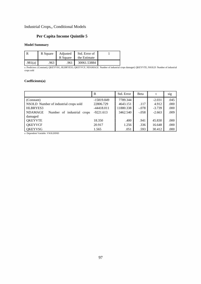
97
Industrial Crops,, Conditional Models
Per Capita Income Quintile 5
Model Summary
R R Square AdjustedR Square
Std. Error ofthe Estimate
1
.981(a) .963 .961 30061.53884a Predictors: (Constant), QKEYVSG, HLBRYES3, QKEYVCF, NDAMAGE Number of industrial crops damaged, QKEYVTE, NSOLD Number of industrialcrops sold
Coefficients(a)
B Std. Error Beta t sig
(Constant) -15819.849 7789.344 -2.031 .045NSOLD Number of industrial crops sold 22806.729 4643.151 .117 4.912 .000HLBRYES3 -44418.011 11880.338 -.078 -3.739 .000NDAMAGE Number of industrial cropsdamaged
-9221.613 3462.540 -.058 -2.663 .009
QKEYVTE 18.350 .400 .941 45.830 .000QKEYVCF 20.917 1.256 .336 16.648 .000QKEYVSG 1.565 .051 .593 30.412 .000
a Dependent Variable: VSOLDIND

98
F. Livestock, Conditional Models
Per Capita Income Quintile 1
Model Summary
R R Square AdjustedR Square
Std. Error ofthe Estimate
1
.752(a) .566 .538 10752.97770a Predictors: (Constant), INT_LCOW, NCBULL, FEMHEAD female headed hh, PVASST02 Unstandardized Predicted Value, NSOLD_LV, SCHHEAD2,SOLDEGG, SOLDCBUL, NCCOW, NLCOW, INT_CHIC, NADULT2, NSOLD_LP, INT_CCOW
Coefficients(a)
B Std. Error Beta t sig
(Constant) 2536.948 1285.551 1.973 .050NADULT2 369.362 311.439 .071 1.186 .237SCHHEAD2 -732.158 289.997 -.141 -2.525 .012PVASST02 Unstandardized Predicted Value .017 .008 .091 1.985 .048FEMHEAD female headed hh -3103.275 1834.782 -.081 -1.691 .092NSOLD_LP 7481.220 1780.279 .310 4.202 .000NSOLD_LV 6812.023 1186.609 .281 5.741 .000NCBULL -10497.346 2751.192 -.202 -3.816 .000NLCOW 1823.542 337.652 .284 5.401 .000NCCOW 1654.251 919.257 .146 1.800 .073SOLDCBUL 10788.129 4932.818 .108 2.187 .030SOLDEGG -12728.094 3229.263 -.300 -3.941 .000INT_CCOW 4035.854 1154.473 .307 3.496 .001INT_CHIC 860.707 205.981 .245 4.179 .000INT_LCOW -1027.973 674.158 -.088 -1.525 .129
a Dependent Variable: VNET_LV Net value livestock income

99
Livestock, Conditional Models
Per Capita Income Quintile 2
Model Summary
R R Square AdjustedR Square
Std. Error of theEstimate
1
.711(a) .506 .484 23923.76314a Predictors: (Constant), INT_CHIC, NSOLD_LV, INT_GCOW, ORDCOMP order interacted with ecompare, NPROD_LP, INT_CCOW, SOLDMK, SCCOW3,NGCALF, NSOLD_LP
Coefficients(a)
B Std. Error Beta t sig
(Constant) -6952.250 5286.945 -1.315 .190ORDCOMP order interacted with ecompare 874.219 364.354 .119 2.399 .017NPROD_LP 4965.036 3032.608 .090 1.637 .103NSOLD_LP -4785.752 4017.785 -.102 -1.191 .235NSOLD_LV 5008.167 1980.080 .137 2.529 .012NGCALF 10976.187 3875.738 .205 2.832 .005SCCOW3 32525.657 7168.606 .267 4.537 .000SOLDMK 10326.907 5162.643 .155 2.000 .047INT_GCOW 5661.144 2457.878 .169 2.303 .022INT_CCOW 4803.523 1266.784 .227 3.792 .000INT_CHIC 799.611 277.171 .162 2.885 .004
a Dependent Variable: VNET_LV Net value livestock income

100
Livestock, Conditional Models
Per Capita Income Quintile 3
Model Summary
R R Square AdjustedR Square
Std. Error ofthe Estimate
1
.688(a) .473 .439 23765.04312a Predictors: (Constant), INT_GCOW, NCBULL, NSOLD_LV, SCCOW1, NLCALF, NGBULL, ORDCOMP2, NPROD_LP, SOLDCBUL, SCCOW3, INT_CCOW,NPRODLP3, NGCALF, NGCOW
Coefficients(a)
B Std. Error Beta t sig
(Constant) -991.746 4642.764 -.214 .831ORDCOMP2 -778.958 450.218 -.092 -1.730 .085NPROD_LP 6778.670 2591.269 .141 2.616 .010NPRODLP3 -7177.495 2403.670 -.199 -2.986 .003NSOLD_LV 3850.780 2051.914 .112 1.877 .062SOLDCBUL 33705.204 13381.824 .138 2.519 .012NGCALF 30538.982 4604.005 .467 6.633 .000NLCALF 5267.392 947.816 .294 5.557 .000NGBULL 45425.669 12799.888 .186 3.549 .000NCBULL 6402.490 2721.498 .135 2.353 .020NGCOW -10223.280 7166.297 -.373 -1.427 .155SCCOW3 28596.216 8335.255 .206 3.431 .001SCCOW1 25424.114 14066.845 .090 1.807 .072INT_CCOW 3657.230 1440.444 .160 2.539 .012INT_GCOW 10563.705 7229.230 .382 1.461 .145
a Dependent Variable: VNET_LV Net value livestock income

101
Livestock, Conditional Models
Per Capita Income Quintile 4
Model Summary
R R Square AdjustedR Square
Std. Error of theEstimate
1
.684(a) .468 .436 31279.17231a Predictors: (Constant), INT_GCOW, SCBUL2, SGCOW2, INT_CHIC, NLCALF, NSOLD_LV, SCH_HEAD years of schooling for hh head, NCCALF, NADULT# of adults in hh, SCHHEAD2, NSHEEP, SOLDEGG, NGCALF
Coefficients(a)
B Std. Error Beta t sig
(Constant) -4446.887 6375.741 -.697 .486NADULT # of adults in hh 1684.730 810.115 .110 2.080 .039SCH_HEAD years of schooling for hh head 1200.354 488.666 .128 2.456 .015SCHHEAD2 -2010.631 698.741 -.156 -2.878 .004NGCALF 13543.950 4131.466 .252 3.278 .001NCCALF 8031.713 1772.908 .247 4.530 .000NLCALF 3393.334 1087.780 .180 3.120 .002NSHEEP -1172.572 482.072 -.142 -2.432 .016NSOLD_LV 5560.323 2109.877 .139 2.635 .009SGCOW2 117690.005 32338.110 .184 3.639 .000SCBUL2 73594.305 32829.109 .115 2.242 .026SOLDEGG -12312.502 7156.791 -.120 -1.720 .087INT_CHIC 1598.172 327.237 .341 4.884 .000INT_GCOW 8828.408 2641.618 .251 3.342 .001
a Dependent Variable: VNET_LV Net value livestock income

102
Livestock, Conditional Models
Per Capita Income Quintile 5
Model Summary
R R Square AdjustedR Square
Std. Error of theEstimate
1
.917(a) .841 .831 43653.41115a Predictors: (Constant), INT_CCOW, NCHICK, FEMHEAD female headed hh, NLCALF, SGBUL3, NSOLD_LV, SCHHEAD3, INT_GCOW, NSHEEP,NCCALF, SGCOW3, ORDCOMP3, SOLDMK3, NPRODLP3
Coefficients(a)
B Std. Error Beta t sig
(Constant) -6687.529 4959.748 -1.348 .179ORDCOMP3 3268.896 975.706 .195 3.350 .001SCHHEAD3 -3456.407 913.436 -.161 -3.784 .000FEMHEAD female headed hh 15997.283 9515.445 .047 1.681 .094NPRODLP3 -18574.029 7716.602 -.179 -2.407 .017NCHICK 751.004 31.666 .679 23.716 .000NCCALF 6326.159 1240.151 .192 5.101 .000NSHEEP -1652.254 674.187 -.081 -2.451 .015NLCALF 6221.551 2317.906 .080 2.684 .008NSOLD_LV 16181.244 2892.993 .171 5.593 .000SGCOW3 44778.080 16150.054 .115 2.773 .006SGBUL3 64367.651 25077.813 .088 2.567 .011SOLDMK3 24627.688 14193.132 .106 1.735 .084INT_GCOW 16923.498 1920.047 .312 8.814 .000INT_CCOW 4010.643 1640.543 .099 2.445 .015
a Dependent Variable: VNET_LV Net value livestock income

103
G. Informal Off-Farm, Conditional Models
Per Capita Income Quintile 1
Model Summary
R R Square AdjustedR Square
Std. Error of theEstimate
1
.707(a) .500 .448 15323.68940a Predictors: (Constant), MTHCARP, MINE mining business, MTHTOUT, MTHCLOTH, MTHBIKE, MTHBREW, PVASST02 Unstandardized Predicted Value,ORDCOMP2, NMTHS # of months hh had income from informal activities, NPEOPLE3, NADULT1, NPEOPLE2, PVASSET2, TOUT Tout, CLOTHES clothesbusiness
Coefficients(a)
B Std. Error Beta t sig
(Constant) -11885.108 4217.677 -2.818 .006NMTHS # of months hh had income frominformal activities
1447.401 363.355 .255 3.983 .000
NPEOPLE2 9090.627 3522.396 .275 2.581 .011NPEOPLE3 9585.545 1933.357 .341 4.958 .000NADULT1 2416.567 525.250 .336 4.601 .000PVASST02 Unstandardized Predicted Value .056 .034 .122 1.643 .103PVASSET2 .118 .063 .202 1.863 .064ORDCOMP2 -1384.592 609.577 -.286 -2.271 .025MINE mining business 26462.786 11085.274 .143 2.387 .018TOUT Tout -167767.462 68326.659 -1.270 -2.455 .015CLOTHES clothes business 217584.409 71449.188 1.647 3.045 .003MTHCLOTH -18625.641 6492.618 -1.561 -2.869 .005MTHBREW 759.550 433.977 .111 1.750 .082MTHTOUT 17823.662 6015.718 1.528 2.963 .004MTHBIKE 823.697 636.063 .079 1.295 .197MTHCARP 1193.821 638.875 .115 1.869 .064
a Dependent Variable: VINFORM earnings from all informal off-farm activities

104
Informal Off-Farm, Conditional Models
Per Capita Income Quintile 2
Model Summary
R R Square AdjustedR Square
Std. Error of theEstimate
1
.535(a) .286 .249 37420.23227a Predictors: (Constant), MANDAS mandasi cakes, MTHHAWK, POSHO posho mill, ORDCOMP3, NMTHS # of months hh had income from informal activities,NADULT # of adults in hh, MTHTRANS, MTHMAND
Coefficients(a)
B Std. Error Beta t sig
(Constant) -11520.243 10935.552 -1.053 .294NMTHS # of months hh had income frominformal activities
2687.649 852.214 0.221 3.154 .002
NADULT # of adults in hh 2263.765 1105.671 .148 2.047 .042ORDCOMP3 1941.445 1021.036 .132 1.901 .059MTHTRANS 7023.604 3508.347 .153 2.002 .047MTHMAND -184175.958 41846.967 -9.568 -4.401 .000MTHHAWK -3339.258 2148.704 -.109 -1.554 .122POSHO posho mill 36418.724 22304.141 .114 1.633 .105MANDAS mandasi cakes 2221781.518 494069.29
19.749 4.497 .000
a Dependent Variable: VINFORM earnings from all informal off-farm activities

105
Informal Off-Farm, Conditional Models
Per Capita Income Quintile 3
Model Summary
R R Square AdjustedR Square
Std. Error of theEstimate
1
.636(a) .404 .365 36696.46931a Predictors: (Constant), JAGG jaggery, MTHHAWK, MTHMASON, NMTHS3, NMTHS # of months hh had income from informal activities, SCHHEAD1,NADULT # of adults in hh, PVASSET2, NPEOPLE1, WAGE2
Coefficients(a)
B Std. Error Beta t sig
(Constant) -21661.619 11089.290 -1.953 .053NADULT # of adults in hh 3649.858 1151.224 .220 3.170 .002SCHHEAD1 -3692.826 1129.675 -.259 -3.269 .001PVASSET2 .255 .082 .300 3.120 .002NMTHS # of months hh had income frominformal activities
2347.523 949.380 .179 2.473 .015
NMTHS3 1196.619 836.728 .114 1.430 .155NPEOPLE1 16519.782 4089.928 .349 4.039 .000WAGE2 -434.131 192.126 -.248 -2.260 .025MTHHAWK 8294.315 1862.991 .297 4.452 .000MTHMASON 2170.847 1008.057 .145 2.153 .033JAGG jaggery 94031.918 38759.530 .160 2.426 .016
a Dependent Variable: VINFORM earnings from all informal off-farm activities

106
Informal Off-Farm, Conditional Models
Per Capita Income Quintile 4
Model Summary
R R Square AdjustedR Square
Std. Error ofthe Estimate
1
.613(a) .376 .343 62766.88319a Predictors: (Constant), MTHTIMB, MINE mining business, FEMHEAD3, SCHHEAD1, NPEOPLE # of people earning informal income, ORDCOMP orderinteracted with cash income, NMTHS3, PVASSET1
Coefficients(a)
B Std. Error Beta t sig
(Constant) -27138.668 18002.063 -1.508 .134SCHHEAD1 -2572.830 1631.123 -.121 -1.577 .117PVASSET1 .166 .043 .300 3.891 .000ORDCOMP order interacted with cash income 3251.951 1696.004 .133 1.917 .057NPEOPLE # of people earning informal income 23386.390 7475.486 .203 3.128 .002NMTHS3 5075.361 1062.070 .341 4.779 .000FEMHEAD3 -82493.146 32982.719 -.166 -2.501 .013MINE mining business 248303.584 66204.167 .252 3.751 .000MTHTIMB 9504.631 3798.038 .163 2.503 .013
a Dependent Variable: VINFORM earnings from all informal off-farm activities

107
Informal Off-Farm, Conditional Models
Per Capita Income Quintile 5
Model Summary
R R Square AdjustedR Square
Std. Error of theEstimate
1
.701(a) .491 .446 115820.35833a Predictors: (Constant), CARP carpentry, PVASST02 Unstandardized Predicted Value, MTHJAGG, MTHDRIVE, MASON masonry business, FEMHEAD3,MTHRET, CLOTHES clothes business, MTHAGTRD, SCHHEAD3, MTHTIMB, ORDCOMP order interacted with cash income, PVASSET1
Coefficients(a)
B Std. Error Beta t sig
(Constant) -134631.380 28478.984 -4.727 .000ORDCOMP order interacted with cash income 15689.930 2865.957 .355 5.475 .000PVASST02 Unstandardized Predicted Value .150 .036 .286 4.217 .000PVASSET1 -.103 .060 -.113 -1.705 .090FEMHEAD3 -113641.348 55290.589 -.127 -2.055 .042SCHHEAD3 3751.256 2123.489 .112 1.767 .079MTHTIMB 24383.343 4872.939 .317 5.004 .000MTHDRIVE 10197.891 4417.743 .137 2.308 .022MTHJAGG 18327.899 7016.766 .157 2.612 .010MTHAGTRD 5142.097 2192.727 .142 2.345 .020MTHRET 3716.705 1930.822 .120 1.925 .056CLOTHES clothes business 67797.242 43328.296 .095 1.565 .120MASON masonry business 87661.476 59618.272 .088 1.470 .144CARP carpentry 241495.089 88435.082 .172 2.731 .007
a Dependent Variable: VINFORM earnings from all informal off-farm activities

108
H. Salaries and Remittances, Conditional Models
Per Capita Income Quintile 1
Model Summary
R R Square AdjustedR Square
Std. Error of theEstimate
1
.812(a) .659 .628 13100.15478a Predictors: (Constant), MTHIND, MTHSHOP, MTHCLERK, MTHBANK, ORDCOMP order interacted with ecompare, SCH_HEAD years of schooling forhh head, WAGERATE Daily wagerate, NMTHS # of months hh had income from sal or remit, MTHFARM, MTHPENS, NMTHS1, MTHREMIT, NPEOPLE1
Coefficients(a)
B Std. Error Beta t sig
(Constant) -13728.216 4546.908 -3.019 .003ORDCOMP order interacted with ecompare 1257.135 333.895 .199 3.765 .000NMTHS # of months hh had income from salor remit
2549.558 337.135 .530 7.562 .000
NMTHS1 1788.611 525.751 .312 3.402 .001NPEOPLE1 -9827.144 3831.283 -.288 -2.565 .011WAGERATE Daily wagerate 98.252 47.840 .137 2.054 .042SCH_HEAD years of schooling for hh head 879.848 311.647 .150 2.823 .005MTHREMIT -2269.127 301.423 -.523 -7.528 .000MTHCLERK 5022.872 1037.656 .270 4.841 .000MTHSHOP 7689.606 1385.334 .345 5.551 .000MTHFARM -1593.424 513.020 -.174 -3.106 .002MTHPENS -973.811 628.458 -.087 -1.550 .123MTHBANK 1553.722 680.036 .120 2.285 .024MTHIND 1112.257 510.108 .120 2.180 .031
a Dependent Variable: VSALREM earnings from all salary and remittance

109
Salaries and Remittances, Conditional Models
Per Capita Income Quintile 2
Model Summary
R R Square AdjustedR Square
Std. Error of theEstimate
1
.693(a) .481 .448 26605.22460a Predictors: (Constant), MTHCIVIL, MTHPOL, MTHCLERK, MTHIND, MTHTEACH, NPEOPLE # of people earning sal or remit, NMTHS # of months hhhad income from sal or remit, ORDCOMP order interacted with ecompare, MTHREMIT
Coefficients(a)
B Std. Error Beta t sig
(Constant) -33979.180 8957.251 -3.793 .000ORDCOMP order interacted with ecompare 2990.226 644.458 .306 4.640 .000NPEOPLE # of people earning sal or remit 10337.267 4185.500 .161 2.470 .015NMTHS # of months hh had income from salor remit
2182.949 656.738 .232 3.324 .001
MTHREMIT -1025.926 475.840 -.159 -2.156 .033MTHPOL 4237.538 1213.430 .226 3.492 .001MTHTEACH 2172.809 686.436 .202 3.165 .002MTHCLERK 2231.012 890.693 .158 2.505 .013MTHIND 1890.490 835.276 .149 2.263 .025MTHCIVIL 4845.734 2252.690 .130 2.151 .033
a Dependent Variable: VSALREM earnings from all salary and remittance

110
Salaries and Remittances, Conditional Models
Per Capita Income Quintile 3
Model Summary
R R Square AdjustedR Square
Std. Error of theEstimate
1
.815(a) .664 .620 33493.96355a Predictors: (Constant), MTHPOL, ORDCOMP order interacted with ecompare, MTHCLERK, NPEOPLE3, NMTHS # of months hh had income from sal orremit, MTHDRIVE, MTHLEC, PVASST02 Unstandardized Predicted Value, MTHIND, NPEOPLE2, MTHREMIT, FEMHEAD3, MTHTEACH, SCHHEAD2,SCHHEAD3, ZONE2, ORDCOMP3, ZONE3
Coefficients(a)
B Std. Error Beta t sig
(Constant) -61769.281 13705.392 -4.507 .000ORDCOMP order interacted with ecompare 4922.440 949.658 .335 5.183 .000ORDCOMP3 -2714.116 1821.310 -.234 -1.490 .138PVASST02 Unstandardized Predicted Value .031 .015 .107 2.032 .044FEMHEAD3 60587.645 18365.337 .197 3.299 .001SCHHEAD2 2866.092 1446.366 .182 1.982 .050SCHHEAD3 6977.398 1577.497 .514 4.423 .000NPEOPLE2 44316.014 8848.375 .504 5.008 .000NPEOPLE3 46453.242 13825.631 .459 3.360 .001NMTHS # of months hh had income from sal orremit
4757.672 953.254 .285 4.991 .000
MTHDRIVE 4630.999 969.349 .258 4.777 .000MTHTEACH 2457.868 783.567 .182 3.137 .002ZONE2 -72614.390 16040.725 -.548 -4.527 .000ZONE3 -87033.955 26730.287 -.677 -3.256 .001MTHIND 2512.816 1060.242 .130 2.370 .019MTHCLERK 2183.492 1190.509 .103 1.834 .069MTHLEC -6593.321 2927.426 -.117 -2.252 .026MTHREMIT -1100.093 583.739 -.112 -1.885 .062MTHPOL 4290.148 2822.368 .076 1.520 .131
a Dependent Variable: VSALREM earnings from all salary and remittance

111
Salaries and Remittances, Conditional Models
Per Capita Income Quintile 4
Model Summary
R R Square AdjustedR Square
Std. Error of theEstimate
1
.698(a) .487 .452 51115.01480a Predictors: (Constant), MTHTEACH, SCHHEAD1, MTHSALES, NPEOPLE # of people earning sal or remit, MTHFARM, NMTHS # of months hh had incomefrom sal or remit, ORDCOMP order interacted with ecompare, MTHREMIT, SCH_HEAD years of schooling for hh head, ZONE1
Coefficients(a)
B Std. Error Beta t sig
(Constant) -80635.725 17886.578 -4.508 .000ORDCOMP order interacted with ecompare 2983.035 1047.050 .189 2.849 .005SCH_HEAD years of schooling for hh head 1779.469 1176.256 .118 1.513 .133SCHHEAD1 5976.984 2616.988 .317 2.284 .024ZONE1 -40307.939 23826.004 -.222 -1.692 .093NPEOPLE # of people earning sal or remit 40497.952 7555.627 .350 5.360 .000NMTHS # of months hh had income from salor remit
4816.867 1470.320 .226 3.276 .001
MTHREMIT -2474.435 934.888 -.183 -2.647 .009MTHFARM -5438.789 2050.378 -.168 -2.653 .009MTHSALES 3347.529 1843.482 .113 1.816 .071MTHTEACH 2055.285 985.437 .143 2.086 .039
a Dependent Variable: VSALREM earnings from all salary and remittance

112
Salaries and Remittances, Conditional Models
Per Capita Income Quintile 5
Model Summary
R R Square AdjustedR Square
Std. Error of theEstimate
1
.840(a) .706 .677 62009.49880a Predictors: (Constant), ZONE2, NMTHS # of months hh had income from sal or remit, MTHMGR, MTHLEC, MTHBANK, MTHPOL, MTHPENS,MTHREMIT, NPEOPLE1, PVASST02 Unstandardized Predicted Value, NPEOPLE # of people earning sal or remit, SCH_HEAD years of schooling for hh head,ORDCOMP1, NPEOPLE2
Coefficients(a)
B Std. Error Beta t sig
(Constant) -138463.686 23560.279 -5.877 .000ORDCOMP1 6101.218 2397.505 .297 2.545 .012PVASST02 Unstandardized Predicted Value .033 .019 .092 1.727 .086NPEOPLE # of people earning sal or remit 87405.544 7689.324 .647 11.367 .000NPEOPLE1 -56402.568 18483.930 -.362 -3.051 .003NPEOPLE2 -79117.668 19562.942 -.480 -4.044 .000SCH_HEAD years of schooling for hh head 4336.894 1286.250 .193 3.372 .001NMTHS # of months hh had income from sal orremit
6604.217 1904.267 .169 3.468 .001
MTHMGR 11107.376 2148.505 .255 5.170 .000MTHLEC 10286.180 2804.355 .180 3.668 .000MTHBANK 6468.358 2078.183 .148 3.113 .002MTHREMIT -3288.065 1093.811 -.172 -3.006 .003MTHPENS -4116.847 1520.631 -.130 -2.707 .008MTHPOL 9021.798 4522.343 .112 1.995 .048ZONE2 83747.872 36380.611 .247 2.302 .023
a Dependent Variable: VSALREM earnings from all salary and remittance
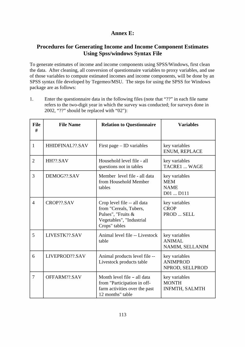
113
Annex E:
Procedures for Generating Income and Income Component EstimatesUsing Spss/windows Syntax File
To generate estimates of income and income components using SPSS/Windows, first cleanthe data. After cleaning, all conversion of questionnaire variables to proxy variables, and useof those variables to compute estimated incomes and income components, will be done by anSPSS syntax file developed by Tegemeo/MSU. The steps for using the SPSS for Windowspackage are as follows:
1. Enter the questionnaire data in the following files (note that “??” in each file namerefers to the two-digit year in which the survey was conducted; for surveys done in2002, “??” should be replaced with “02"):
File#
File Name Relation to Questionnaire Variables
1 HHIDFINAL??.SAV First page – ID variables key variablesENUM, REPLACE
2 HH??.SAV Household level file - allquestions not in tables
key variablesTACRE1 ... WAGE
3 DEMOG??.SAV Member level file - all datafrom Household Membertables
key variablesMEMNAMED01 ... D111
4 CROP??.SAV Crop level file -- all datafrom "Cereals, Tubers,Pulses", "Fruits &Vegetables", "IndustrialCrops" tables
key variablesCROPPROD ... SELL
5 LIVESTK??.SAV Animal level file -- Livestocktable
key variablesANIMALNAMIM, SELLANIM
6 LIVEPROD??.SAV Animal products level file --Livestock products table
key variablesANIMPRODNPROD, SELLPROD
7 OFFARM??.SAV Month level file � all datafrom "Participation in off-farm activities over the past12 months" table
key variablesMONTHINFMTH, SALMTH

File#
File Name Relation to Questionnaire Variables
114
8 BUSLAB??.SAV Activity level file � data fromleft hand portion of "Businessand informal off-farmactivities, and salaried wagelabour" table
key variablesACTINFINFORMAL
9 SALWAGE??.SAV Activity level file � data fromright hand portion of"Business and informal off-farm activities, and salariedwage labour" table
key variablesACTSALSALARIED
10 ASSET??.SAV All data from assets table key variablesITEMQTY
12 ECACT??.SAV All data from "Importance ofIncome Sources" Table
key variablesECONACTORDER
2. Save these uncleaned files in a folder of your choice. This will be your copy of theoriginal, uncleaned data, which should not be changed.
3. Create the folder c:\proxy??\incprox\data and copy all 12 uncleaned files to it. As inthe file naming conventions in the table above, replace "??" with the two digit year ofthe survey, e.g., "02" if the survey was conducted in 2002.
4. Clean the files in c:\proxy??\incprox\data using procedures your institution hasdeveloped with other surveys, and save the files to the same names. You will nowhave uncleaned, original data in a folder of your choice, and cleaned data inc:\proxy??\incprox\data.
5. Create the folder c:\proxy??\incprox\syntax and copy the fileIncproxEstimateKenya.sps to it. Tegemeo/MSU will provide you with a copy of thisfile upon request.
6 Run IncproxEstimateKenya.sps. This file will create all required proxy variables andgenerate income results, saving them to the file IncomeKenya.sav. It will also delivermean and median values for household income and income components in the SPSSOutput Navigator.