developing an application test bed for hydrological

Developing an Application Test Bed for Hydrological Modelling of Climate Change Impacts: Cox Creek

Catchment, Mount Lofty Ranges

Werner AD, Jakovovic D, Ordens CM, Green G, Woods J, Fleming N, Alcoe D

Goyder Institute for Water Research Technical Report Series No. 14/28

www.goyderinstitute.org

Goyder Institute for Water Research Technical Report Series ISSN: 1839-2725 The Goyder Institute for Water Research is a partnership between the South Australian Government through the Department of Environment, Water and Natural Resources, CSIRO, Flinders University, the University of Adelaide and the University of South Australia. The Institute will enhance the South Australian Government’s capacity to develop and deliver science-based policy solutions in water management. It brings together the best scientists and researchers across Australia to provide expert and independent scientific advice to inform good government water policy and identify future threats and opportunities to water security.

The following Associate organisations contributed to this report:

Enquires should be addressed to: Goyder Institute for Water Research

Level 1, Torrens Building 220 Victoria Square, Adelaide, SA, 5000 tel: 08-8303 8952 e-mail: [email protected]

Citation: Werner AD, Jakovovic D, Ordens CM, Green G, Woods J, Fleming N, Alcoe D, 2014, Developing an application test bed for hydrological modelling of climate change impacts: Cox Creek Catchment, Mount Lofty Ranges, Goyder Institute for Water Research Technical Report Series No. 14/28, Adelaide, South Australia. Copyright: © 2014 [Flinders University] To the extent permitted by law, all rights are reserved and no part of this publication covered by copyright may be reproduced or copied in any form or by any means except with the written permission of Flinders University.

Disclaimer: The Participants advise that the information contained in this publication comprises general statements based on scientific research and does not warrant or represent the completeness of any information or material in this publication. Acknowledgments: The authors appreciate the review comments of Nikki Harrington and Matt Gibbs that assisted in improving this report. John Hutson provided extensive assistance with LEACHM modelling, and Matt Knowling offered useful guidance on the MODFLOW calibration methodology.

Executive Summary

The Goyder Institute for Water Research (GIWR) project ‘An agreed set of climate change projections for South Australia’ was established to produce a benchmark set of downscaled climate projections for the eight natural resource management regions in South Australia. The fourth task in the GIWR project requires the development of a suite of hydrological models to serve as a test bed for the downscaled climate change projections. The Onkaparinga River catchment was identified as the primary case study area for hydrological modelling. This report outlines the construction of three hydrological models of the northern 15.6 km2 of the Cox Creek sub-catchment, including: (1) a MODFLOW groundwater model, (2) a LEACHM recharge model, and (3) a SOURCE (GR4J) catchment runoff model. The models were develop through a collaborative effort involving Flinders University, the Department of Environment, Water and Natural Resources (DEWNR), and the South Australian Research and Development Institute (SARDI), who each led the construction of the groundwater, recharge and runoff models, respectively. The Cox Creek catchment has steep topography and experiences a Mediterranean-type climate. The higher rainfall of autumn and winter leads to increasing stream flow from April to August, declining stream flow from September to December, and base flow conditions between December and March. Land use within the study area is diverse, and includes a significant reliance on groundwater for irrigation and other water demands. Groundwater resources are contained within fractured rock sediments, which vary widely in permeability, storage capacity and water quality. Groundwater flow patterns are highly dependent on surface water-groundwater interaction, whereby recharge from elevated areas flows towards generally gaining streams. The GR4J model of SOURCE was used to simulate stream flow in response to daily rainfall and potential evapotranspiration. The study area was subdivided into 36 sub-catchments, and model calibration was based on the prediction of stream flow (1975-2004) at three stream gauging stations. A reasonable match was obtained using parameters that are generally consistent with previous GR4J studies. The LEACHM model also uses rainfall and potential evapotranspiration, in addition to soil, vegetation, topography and land use characteristics to simulate surface runoff and recharge through 1D soil profiles, and crop demands for irrigation. The LEACHM results were compared to field-based estimates of groundwater recharge and independent appraisals of irrigation rates. Groundwater flow was simulated using MODFLOW, which adopted recharge and pumping predictions from LEACHM, and hydrogeological knowledge of the study area to simulate groundwater changes during 1975-2004. MODFLOW calibration involved both steady-state and transient models, which were compared to observed groundwater heads. Inter-model comparison, involving evaluation of internal fluxes within each of the models, was an important aspect of the current study. For example, LEACHM and GR4J were compared in terms of groundwater recharge and surface runoff, and groundwater-surface water interactions in MODFLOW and GR4J were compared, amongst other inter-dependencies between the three models. The suite of hydrological models was used to test four future climate scenarios, which were based on the projections of

two of the 15 available climate models, as developed during earlier phases of the GIWR project. The results of catchment runoff modelling using GR4J indicate that, on average, 1092 mm/year of rainfall in the Cox Creek catchment led to 368 mm/year of stream flow, with the remainder lost to evapotranspiration and aquifer discharge. Groundwater recharge within GR4J was 143 mm/year. LEACHM produced an average recharge of 115 mm/year and groundwater pumping for irrigation of 76 mm/year. LEACHM’s surface runoff was 310 mm/year. Given the difference in conceptual models that underpin LEACHM and GR4J, the closeness of the respective recharge and surface runoff estimates was encouraging. The MODFLOW model results highlight the significant effects of groundwater pumping, which accounts for over half of the rainfall recharge to the system. The model predicted that inflows from neighbouring aquifers and losses of groundwater due to shallow watertables are probably important components of the catchment water balance. The four climate change scenarios involved lower future rainfall compared to historical values (i.e., projected rainfall averages for the four scenarios ranged from 956 to 1031 mm/year, whereas the average historical rainfall was 1033 mm/year). Under projected rainfall and potential evapotranspiration, LEACHM predicted that recharge is significantly more impacted by climate change than runoff. That is, recharge declined by between 35 and 44%, whereas surface runoff changed between +1% and -7%. LEACHM-predicted irrigation demand increased significantly, i.e., by 57-70% relative to historical values. As expected, the MODFLOW-simulated response of the groundwater system to higher pumping and reduced recharge (as predicted by LEACHM) under the four climate scenarios involved significant reductions (up to 10 m) in groundwater levels within the Cox Creek aquifer. The project offered important insights into the development of multiple hydrological models to simulate catchment flow processes and their response to predicted climate change. These include: (1) regular re-development and re-calibration of the hydrological models was necessary to produce consistent water fluxes across the three models, (2) achieving flow consistency within the modelling suite was a significant challenge, requiring close cooperation, frequent iteration, and regular communication between the three collaboration partners, (3) projected climate change is likely to produce significantly lower recharge and falling groundwater levels, but largely unchanged surface runoff in the Cox Creek catchment, and (4) the variables produced by the GIWR project for future climate projections were provided in a suitable format for input into the three hydrological models used in this study, albeit careful selection of climate scenarios was needed to limit modelling simulations to a manageable number.

Table of contents

1. Introduction ............................................................................................................... 1

2. Site description ........................................................................................................ 3

2.1 Location and Topography .............................................................................. 3

2.2 Surface Hydrology ........................................................................................... 5 2.3 Land Use .......................................................................................................... 5 2.4 Regional Hydrogeology .................................................................................. 6

2.5 Groundwater Levels ........................................................................................ 8 2.6 Irrigation and Groundwater Pumping ......................................................... 10

3. Methods .................................................................................................................. 12 3.1 SOURCE Model Development .................................................................... 12

3.1.1 GR4J Model Structure .......................................................................... 12 3.1.2 Implementation of GR4J ...................................................................... 14

3.2 LEACHM Model Development .................................................................... 18

3.2.1 Modelling Assumptions ........................................................................ 19 3.2.2 Validation of Groundwater Recharge Models ................................... 20

3.2.3 LEACHM-GIS Modelling Framework ................................................. 21

3.2.4 Soil Type ................................................................................................. 23

3.2.5 Land Use, Irrigation and Vegetation ................................................... 24

3.2.6 Climate Parameters .............................................................................. 26 3.2.7 Land Slope ............................................................................................. 26

3.2.8 Aggregation of Spatial Variables in the LEACHMG Model ............. 27 3.3 MODFLOW Model Development ................................................................ 28

3.3.1 Code Selection ...................................................................................... 28 3.3.2 Model Architecture and Numerical Options ...................................... 28

3.3.3 Aquifer Hydraulic Parameters ............................................................. 30 3.3.4 Model Boundaries and Stresses ......................................................... 31

3.3.5 Calibration .............................................................................................. 32

3.4 Inter-Model Comparisons ............................................................................. 33

3.5 Predictions of Climate Change (DEWNR) ................................................. 36

4. Results .................................................................................................................... 38 4.1 SOURCE ........................................................................................................ 38

4.3 MODFLOW ..................................................................................................... 42 4.3.1 Steady-state Model Calibration ........................................................... 42 4.3.2 Transient Model Calibration ................................................................. 45

4.4 Inter-Model Comparisons ............................................................................. 47 4.5 Predictions ...................................................................................................... 51

4.5.1 LEACHMG .............................................................................................. 52 4.5.2 MODFLOW ............................................................................................. 54

5. Discussion and Conclusions................................................................................ 57

References ..................................................................................................................... 60

List of figures

Figure 1. Cox Creek Catchment and model area (sourced from Alcoe et al., 2013). .. 4

Figure 2. Long term (47-year) average monthly rainfall and evaporation from Lenswood and long-term (40-year) average monthly stream flow at Uraidla (Cox Creek gauging station A5030526). ............................................................................... 5

Figure 3. Hydrogeological zones, monitored observation wells and extraction wells within the study area of the Cox Creek catchment. ................................................... 6

Figure 4. Spatial distribution of the single-measurement head observations grouped by the year of measurement. ......................................................................................... 9

Figure 5. Interpolated water level contours, based on both the average water level from routinely monitored wells and one-off measurements from a large number of sites. ............................................................................................................................ 10

Figure 6. Structure of the rainfall-runoff model GR4J. See Perrin et al. (2003) for explanation of variables (diagram taken from Perrin et al. (2003)). ...................... 13

Figure 7. GR4J model of Cox Creek catchment with the study area outlined in red, showing the location of flow gauges (contributing areas outlined in green) and the study catchment outlet ........................................................................................... 15

Figure 8. Time periods and Nash-Sutcliffe efficiency values of gauging station data 16

Figure 9. Simulated and observed total flow volumes for gauge A5030526 using two alternative parameter sets, obtained from calibration over the two time periods: 1976 to 1989, and 1994 to 2004. ................................................................................ 17

Figure 10. Schematic of the LEACHM model applied to recharge estimation, where T is transpiration, E is evaporation from bare soil, P is precipitation, I is irrigation, Q is direct runoff, R is recharge and dR is the vegetation rooting depth. ............. 18

Figure 11. Distribution of major soil types. ........................................................................ 22

Figure 12. Distributions of (a) land use and (b) land slope used in recharge modelling. ....................................................................................................................... 23

Figure 13. Model domain, grid and boundary conditions. ............................................... 29 Figure 14. Irrigation areas used to determine pumping from extraction wells. ........... 32

Figure 15. (a) Traditional methodology to catchment simulation using multiple hydrological models, (b) Methodology of the current project. ................................ 36

Figure 16. GR4J schematic and annual water budget for simulations of the Cox Creek study area, based on the model diagram of Kelley and O’Brien (2012). All values are average fluxes (mm/year) for the 30-year period. ................................ 38

Figure 17. Monthly simulated and gauged stream flow, and recharge from 1975 to 2004 at Cox Creek gauging station A5030526. ....................................................... 39

Figure 18. Spatial distribution of modelled recharge rates from LEACHMG. .............. 41

Figure 19. Modelled annual recharge and runoff rates for the study area. The annual rainfall rates are from the Uraidla weather station. .................................................. 42

Figure 20. Steady-state calibration scatter plot. Blue diamonds represent the average heads from monitoring wells and red diamonds represent the single-measurement head observations. The black line represents 1:1 match. ............. 43

Figure 21. Comparison of “observed” (i.e. estimated by SOURCE) and simulated groundwater-stream interaction fluxes from the steady-state model, following calibration in which base flow estimates are not considered. Positive values represent losing stream conditions. ........................................................................... 43

Figure 22. Groundwater contours for the calibrated steady-state model. .................... 45

Figure 23. Hydrograph comparison between modelled and observed water levels. . 46

Figure 24. Transient calibration scatter plot. The black line represents the 1:1 match........................................................................................................................................... 47

Figure 25. Steady-state calibration scatter plots: (a) groundwater heads and (b) stream flux. “Observed flux” values were estimated by SOURCE. The black line represents the 1:1 match. Positive values represent losing stream conditions. . 48

Figure 26. Groundwater contours from the Stage 2 calibrated steady-state model. .. 50

Figure 27. Comparison of: (a) surface runoff and (b) recharge between SOURCE and LEACHM. ................................................................................................................ 51

Figure 28. Comparison of historical and future recharge, runoff and irrigation from LEACHM model. ............................................................................................................ 53

Figure 29. Groundwater level hydrographs at observation wells for the four different scenarios. The “Min” and “Max” lines represent minimum and maximum water levels from the calibrated historical hydrographs. .................................................... 55

List of tables

Table 1. Estimated extraction from wells within the study area (Green and Stewart, 2010). .............................................................................................................................. 10

Table 2. Surface flow gauges in the Cox Creek catchment. .......................................... 15

Table 3. Calibrated GR4J parameters for each data set. ............................................... 16

Table 4. Parameters used in the GR4J rainfall-runoff Source model of Cox Creek, with typical parameter values shown for reference. ................................................ 18

Table 4. Soil types encoded into the Cox Creek catchment LEACHMG model (DWLBC, 2007). ............................................................................................................ 24

Table 5. Land-use classifications encoded into the Cox Creek catchment LEACHMG model............................................................................................................................... 25

Table 6. Classification of land slopes in the Cox Creek catchment LEACHMG model........................................................................................................................................... 27

Table 7. Combinations of parameters in the Cox Creek catchment LEACHMG model........................................................................................................................................... 27

Table 8. Parameters tested in the model. ......................................................................... 30

Table 9. Complementary components within the SOURCE, LEACHM and MODFLOW models used to simulate the Cox Creek catchment hydrology. ....... 35

Table 10. Calibrated hydraulic conductivities. .................................................................. 44

Table 11. Calibrated GHB and RIV conductances. ......................................................... 44

Table 12. Water budget for the Stage 1 calibrated steady-state model. ...................... 44

Table 13. Water balance from the transient calibration. ................................................. 47

Table 14. Calibrated storage parameters. ......................................................................... 47

Table 15. Hydraulic conductivities from the Stage 2 steady-state calibration. ............ 49

Table 16. GHB and RIV conductances from the Stage 2 calibration. ........................... 49

Table 17. The water budget for the calibrated steady-state model when taking into account SOURCE estimates of groundwater-stream flux. ..................................... 49

Table 18. Climate change predictions applied in this project. ........................................ 52

Table 19. Historical and future recharge, runoff and irrigation simulated by LEACHM........................................................................................................................................... 54

Table 20. Water balance from Scenario 1. ....................................................................... 56 Table 21. Water balance from Scenario 2. ....................................................................... 56

Table 22. Water balance from Scenario 3. ....................................................................... 56

Table 23. Water balance from Scenario 4. ....................................................................... 56

1

1. Introduction The Goyder Institute for Water Research (GIWR) project ‘An agreed set of climate change projections for South Australia’ was established to develop a benchmark set of downscaled climate projections for the eight natural resource management regions in South Australia to support proactive responses to climate change in water resource planning and management. Time series of environmental variables, including rainfall, temperature and potential evapotranspiration, have been developed by downscaling projections of a suite of selected global-scale climate models. These data sets have been generated for 193 Bureau of Meteorology (BoM) weather stations distributed throughout South Australia. The climate projections account for observed climate variability and the influence of known climate drivers, and use the most up-to-date climate models from the CMIP5 multi-model ensemble of climate models (Taylor et al., 2012), associated with the IPCC Fifth Assessment Report (AR5) (IPCC, 2013) and Australian climate initiatives. The GIWR project involved four major tasks:

(1) Understanding the key drivers of climate change in South Australia (2) Selection of CMIP5 climate models for regional downscaling and projection (3) Downscaling of climate change projections for locations throughout South

Australia (4) Development of a modelling applications test bed

The emphasis of the work conducted for the applications test bed (task 4) was to provide feedback to the developers of the climate change projections and downscaling (task 3), in addition to developing examples of practical modelling applications. The Onkaparinga River catchment was identified by the Goyder Institute as the primary case study location for this project. Where required for this task, new models were developed that represent the case study catchment or its sub-catchments, such as the Cox Creek catchment. The modelling applications test bed was developed to ensure that the research project outputs comply with the specific needs of end users by ensuring an active technical engagement was established between the research team and key state government agencies, including the Department of Environment, Water and Natural Resources (DEWNR), South Australian Research and Development Institute (SARDI) and SA Water. This activity helped to build capacity in end user agencies and is an important step towards the overall goal of developing an agreed set of climate projections for South Australia, ensuring the downscaled climate projection data sets are suitable for use in resource management modelling applications. The involvement of natural resource management scientists in SA government agencies also aimed to foster a working knowledge of the data sets, including the conditions and qualifiers that are required when applying and interpreting the datasets. The application test bed involved the application of the downscaled climate projection data in a range of hydrological test cases, developed collaboratively between the research partners and state government agencies. These applications included:

2

1. Surface water runoff models of the Onkaparinga River catchment, using the eWater ‘SOURCE’ and ‘GR4J’ catchment runoff models

2. Reservoir water quality models of the Happy Valley Reservoir, applying coupled hydrodynamic and chemical/biological water quality models

3. Daily time-step crop growth models, providing a balance of rainfall, soil water content change, irrigation, transpiration, soil surface evaporation, runoff and drainage for a range of climate and landscape scenarios

4. Surface water and groundwater models representative of the linked surface water runoff, groundwater recharge and groundwater flow processes occurring in the Cox Creek sub-catchment of the primary case study: the Onkaparinga River catchment

The fourth of these test bed applications, including a comparison of the outputs and reconciliation of surface and groundwater models of the Cox Creek sub-catchment under varying climate scenarios is the subject of this report. The remainder of this report is divided into four main sections: Site Description, Methods, Results, and Discussion and Conclusions. The Site Description section defines the Cox Creek study area, and provides a general characterisation of its hydrology. The Methods section outlines approaches for developing hydrological models of the Cox Creek catchment, including its surface domain, aquifer system and soil zone. In this section, strategies for comparing and combining the different models are described. The approach to simulating climate change impacts is also given in the Methods section. The Results section contains simulation outputs and comparisons between models. Important features of the model results and comparative analyses are further explored in the Discussion and Conclusions section, which also offers the key findings of the investigation.

3

2. Site description 2.1 Location and Topography The project area is approximately 20 km east of Adelaide, South Australia, and encompasses the northern 15.6 km2 of the 29.8 km2 Cox Creek catchment in the Western Mount Lofty Ranges (Figure 1). Cox Creek is a tributary of the Onkaparinga River, which has a catchment area of some 554 km2, extending from Mount Torrens in the north to the Gulf St Vincent in the south-west. The southern part of the catchment is not included because there are little data available and the groundwater extraction is small relative to that of the study area. The Cox Creek catchment has a steep topography, particularly along the western boundary, varying in elevation from 700 m AHD (Australian Height Datum) near the Mount Lofty Summit to 320 m AHD at the southern boundary of the catchment. The lowest elevation of the study area is approximately 420 m AHD at the southern boundary, near Woodhouse (Figure 1).

4

Figure 1. Cox Creek Catchment and model area (sourced from Alcoe et al., 2013).

5

2.2 Surface Hydrology The Cox Creek study area has a Mediterranean-type climate with cool, wet winters (June to August) and dry, hot summers (December to February). Average monthly pan evaporation exceeds average monthly rainfall from October to April, as shown in Figure 2. From spring through summer this causes extensive drying of the soil profile.

Figure 2. Long term (47-year) average monthly rainfall and evaporation from Lenswood and long-term (40-year) average monthly stream flow at Uraidla (Cox Creek gauging station A5030526). The onset of autumn rains, combined with reduced evaporation through lower temperatures, causes wetting of the soil profile in autumn and early winter. Continued rainfall after wetting of the soil profile increases stream flow, typically from early winter until late spring. Stream flow is least during late spring and summer, as shown in Figure 2.

2.3 Land Use A range of land uses occupy the area of the upper Cox Creek catchment. In the central and northern part of the upper catchment, where the topography is more subdued than at the edges of the catchment, the land use is dominated by large areas of commercial horticultural production. These include areas of seasonal vegetable production and perennial horticulture such as fruit trees and some vineyards. At the western side of the upper catchment, the topography is very steep and land uses include nature conservation areas (primarily eucalypt forest) and rural residential properties. The eastern edge of the catchment contains a mix of areas of grazing land, large rural residential properties and nature conservation areas. The

6

southern third of the study area is predominantly covered by three main land uses: the suburban residential area of Crafers, the Mount Lofty Botanic Gardens and the Mount Lofty Golf Course.

2.4 Regional Hydrogeology The catchment lies within the Adelaide Geosyncline, which stretches from the Flinders Ranges to Kangaroo Island, and encompasses the Mount Lofty Ranges (Preiss, 1993). The stratigraphic sequences of the Cox Creek catchment are typical of those associated with the Adelaide Geosyncline (Banks, 2010). That is, the geology of the study area is dominated by the Neoproterozoic Burra Group, including the Emeroo Subgroup (Aldgate Sandstone) in the east corner of the catchment, and the Bungarider Subgroup (Woolshed Flat Shale and Stonyfell Quartzite) and Mundollio Subgroup (Basket Range Sandstone) in the north and west parts of the catchment (Banks, 2010). The Mundolllio and Bungarider Subgroups are separated from the Emeroo Subgroup by the Archean Barossa Complex, which covers the centre of the catchment (Figure 3).

Figure 3. Hydrogeological zones, monitored observation wells and extraction wells within the study area of the Cox Creek catchment. Deposits of undifferentiated Quaternary rocks and sediments of Pleistocene and Holocene age are present throughout the catchment along the valleys and

7

depressions (Banks, 2010). Major fault lines occur along the margins of the different geological units. For example, a fault along the margin of the Barossa Complex, traversing in a NE-SW orientation, separates the Basket Range Sandstone, Woolshed Flat Shale and Stonyfell Quartzite from the Barossa Complex (Stewart and Green, 2010). Groundwater in the Cox Creek catchment predominantly flows through fractured rock aquifers, subdivided into the Stonyfell Quartzite, the Woolshed Flat Shale, the Basket Range Sandstone, the Barossa Complex, and the Aldgate Sandstone (Figure 3). Aquifer test data are available only for the Woolshed Flat Shale and Aldgate Sandstone formations. The Stonyfell Quartzite formation is gently south-dipping, comprising feldspathic quartzite, with medium-to-coarse sandstone interbeds (Stewart and Green, 2010). At the western side of the catchment, beneath the Mount Lofty Summit, the Stonyfell Quartzite contains a perched aquifer on top of the Woolshed Flat Shale (Stewart and Green, 2010). Around the southern margin of the catchment, domestic supplies are obtained from this unit. The Woolshed Flat Shale formation consists of shale, sandy shale and grey laminated siltstone (Stewart and Green, 2010). The storage capacity of this unit is mainly a function of fractures and joint development. The presence of pyrite may elevate iron levels and lead to some deterioration in the quality of the water (Stewart and Green, 2010). Aquifer tests at Forreston, approximately 20 km north of the Cox Creek catchment, give a range for the bulk hydraulic conductivity (i.e., the combined hydraulic conductivity of the fractures and porous rock matrix) of 2.1 to 15.9 m/d (Green et al., 2007) for this formation. The Basket Range Sandstone formation consists of coarse-grained, feldspathic, thick-bedded sandstone. Near the top of the unit, a dolomitic siltstone interbed is present (Stewart and Green, 2010). The Basket Range Sandstone aquifer has primary and secondary porosities, which enhance its storage and conductive capabilities. Fractures in this aquifer tend to be widely spaced with large apertures (Banks, 2010). High yields of good quality water are obtainable and the aquifer is used extensively for irrigation purposes (Stewart and Green, 2010). The Barossa Complex is characterised by metamorphic rocks with retrograde metamorphism and minor intrusive granitic dykes. This unit is generally considered to be a poor aquifer with yields not suitable for irrigation purposes (Stewart and Green, 2010). Decomposition of the granitic rocks to clay reduces permeability in the weathered zone and may lead to an increase in the salinity of the groundwater (Stewart and Green, 2010). Compared to the other aquifers in the catchment, the permeability in the Barossa Complex is greatly reduced and there are fewer conductive fractures (Banks, 2010). The Aldgate Sandstone consists of micaceous sandstone and quartzite. This unit is considered to have similar aquifer properties to the Basket Range Sandstone (Stewart and Green, 2010). The bulk hydraulic conductivity of the Aldgate Sandstone was found to be 0.002 to 0.02 m/d from aquifer tests at Mylor, which is approximately 2 km south of the Cox Creek catchment (Green et al., 2007).

8

The regional groundwater flow direction within the Cox Creek catchment is from the elevated areas at the edges of the catchment towards Cox Creek at the topographically lower, central area (Banks, 2010). The orientation of the higher permeability fracture zones relative to the hydraulic gradient is expected to play a major role in the direction of groundwater flow (Cook, 2003). However, there are not sufficient data to assign orientations to hydraulic conductivity in accordance with any anisotropy. Banks (2010) conducted a study of the groundwater-surface water interaction in the area and indicated that groundwater is highly connected to surface water. He concluded that the groundwater contribution to Cox Creek is mainly from the geological units of the Burra Group, whereas the Barossa Complex unit contributes minimally to stream flow.

2.5 Groundwater Levels Eleven observation wells are currently monitored within the study area (Figure 3), as part of the OBSWELL network (www.waterconnect.sa.gov.au) for the Onkaparinga catchment. The majority of the wells (i.e., 8 out of 11) monitor the Basket Range Sandstone aquifer. The Woolshed Flat Shale contains three observation wells, and there are no current monitoring wells in the Stonyfell Quartzite, Barossa Complex and Aldgate Sandstone units. Cox Creek hydrographs are provided in the model calibration section of the report (Section 4.3.2). A regular water level fluctuation of varying magnitude is observed in the wells, presumably arising from the strong seasonality of the rainfall and groundwater extraction. Otherwise, the wells show generally stable long-term trends. Groundwater levels have been recorded on an ad-hoc basis in wells that are not part of the OBSWELL network. For example, single-measurement head observations, obtained soon after well construction, are available for many of the domestic and irrigation wells in the area. Figure 4 shows the spatial distribution of the single-measurement head observations plotted according to the time at which each observation was taken. These were included in the calibration of the model because of the limited coverage of wells that are routinely measured. That is, wells with only sporadic measurements, which are therefore considered to be rather uncertain, provided useful information regarding groundwater level spatial trends in areas where no other information was otherwise available. Wells with only a single measurement were assigned reduced calibration weightings to reflect their higher uncertainty regarding their accuracy and representativeness of the regional conditions, relative to routinely-monitored wells; see Section 3.3.5.

http://www.waterconnect.sa.gov.au/

9

Figure 4. Spatial distribution of the single-measurement head observations grouped by the year of measurement. Figure 5 shows the potentiometric surface obtained from interpolating both single-measurements and time-averaged values from regularly-monitored groundwater wells. Given that the time-frame for head measurements used to develop Figure 5 spans some 35 years, the associated head contours should be considered as approximate only. It can be inferred from Figure 5 that the groundwater flow is from the elevated edges of the catchment towards the main branch of Cox Creek, as expected in a system of steep topography where there are strong steam-groundwater connections. The areas where the contours are parallel to the boundary are considered to indicate that there is significant flow across the boundary, most likely due to exchanges of groundwater with neighbouring systems. Where the contours are perpendicular to the boundary, the boundary is assumed to represent a no-flow limit to the groundwater system. The groundwater flow directions in the proximity of streams, as discernible from the Figure 5 contours, highlight that the major streams in the catchment are predominantly gaining.

10

Figure 5. Interpolated water level contours, based on both the average water level from routinely monitored wells and one-off measurements from a large number of sites.

2.6 Irrigation and Groundwater Pumping Within the study area, horticultural producers, botanic gardens and the golf course all use substantial amounts of irrigation water, particularly during the summer months. Irrigation water for these purposes is drawn from the underlying fractured rock aquifers. Green and Stewart (2010) produced estimates of theoretical crop water use and assumed that irrigation needs were met from groundwater pumping. Based on the distribution of irrigation wells and irrigated land within the study area, they calculated that three of the fractured rock aquifer types (Basket Range Sandstone, Woolshed Flat Shale and Barossa Complex) supplied more than 96% of the regions’ irrigation requirements. The Basket Range Sandstone FRA is by far the largest source of irrigation water (Table 1). Table 1. Estimated extraction from wells within the study area (Green and Stewart, 2010).

Geology type Number of wells Extraction (m3/year)

Stonyfell Quartzite 1 2,736

Woolshed Flat Shale 11 124,256

Basket Range Sandstone 24 490,698

Aldgate Sandstone 2 20,660

Barossa Complex 11 83,967

Total 49 722,317

11

Aside from irrigation, groundwater extraction in the Cox Creek catchment occurs for local domestic and industrial uses. There are 48 known extraction wells in the study area (see Figure 3). The majority of these are located in the Basket Range Sandstone and Woolshed Flat Shale aquifers. There are little data available on extraction volumes, and hence, pumping was estimated by considering the area of irrigation and irrigation practices within the catchment, for the purposes of groundwater modelling (see Section 3.3.4). Within the irrigated areas, the irrigation is expected to enhance contemporary groundwater recharge. This effect is incorporated within the groundwater recharge modelling described in Section 3.2.

12

3. Methods Three models were developed, initially independently, to evaluate the hydrology of the study area: a LEACHM (Hutson et al., 1997) model of groundwater recharge, a SOURCE (Delgado et al., 2012) model of catchment runoff, and a MODFLOW (Harbaugh et al., 2000) groundwater flow model. Conceptually, each model focuses predominantly on a different part of the Cox Creek catchment water cycle. However, there are water balance components that overlap across the different models. Evaluating catchment fluxes that were duplicated within two or three of the models was an important component of this study. The initial construction of each of the models followed a similar general process, involving the usual phases of: (1) amalgamating the relevant data sets, (2) model conceptualisation, (3) prototype model construction, and (4) sensitivity testing, comparison to field measurements, and model calibration. Subsequent to the development of prototype models, several of these activities were repeated during inter-model comparisons, whereby flux components generated as model outputs and/or as internal computations within each model were compared, leading to model redevelopment and adjustment.

3.1 SOURCE Model Development 3.1.1 GR4J Model Structure The purpose of the SOURCE model was to estimate recharge by calibrating surface runoff to recorded flow using one of rainfall-runoff models available within SOURCE. The Cox Creek catchment has proven difficult to calibrate with widely used catchment models such as SIMHYD or AWBM (Fleming et al., 2012). This may be due to the known extensive interaction between surface water and groundwater in the study area. The GR4J model (Perrin et al., 2003) was chosen for this project because it can more effectively simulate stream flow in the study area, and can allocate flow to groundwater exchange through an explicit parameter (x2), which determines water transfer between surface flow and groundwater. GR4J requires relatively simple inputs of rainfall and potential evapotranspiration (PET), and contains only four variables; which simplifies calibration. The model runs on a daily time step. The structure of the model is illustrated in Figure 6.

13

1

2

3

4

5

6

7

8

9

10

11

12

13

14

15

16

17

18

Figure 6. Structure of the rainfall-runoff 19

model GR4J. See Perrin et al. (2003) for 20

explanation of variables (diagram taken 21

from Perrin et al. (2003)). 22

A brief description of processes within the GR4J model follows. Firstly, daily evaporation is subtracted from precipitation to determine either net precipitation or net evaporation. Net precipitation or evaporation adds to or subtracts from the production store (S), which acts as a soil moisture accounting store. The amount of water stored in S affects how much water can enter as net precipitation or leave as net evaporation. Precipitation which is surplus to that entering S (Pn-Ps) goes to a routing function. This is combined with percolation (Perc) from S, the quantity of which is dependent on the amount of water in S. This combined routing precipitation (Pr) is divided into two components according to a fixed split: 90% of Pr is routed by a unit hydrograph UH1, and it then enters a non-linear routing store. The remaining 10% of Pr is routed by a single unit hydrograph UH2. The UH1 hydrograph operates over a shorter time frame than UH2, and simulates quickflow, or direct flow (Qd). The UH2 hydrograph and the routing store produce slow flow, or routed flow (Qr). Qd and Qr are then combined to give stream flow (Q). For a more detailed explanation, see Perrin et al. (2003). In the context of a large catchment (e.g. hundreds of square kilometres), GR4J simulates flow at the catchment outlet. The production store (S) is analogous to the catchment contributing area, in that precipitation entering the soil system is Ps. Surface runoff is the remainder of net precipitation (Pn-Ps). Percolation is added to Pn-Ps to give total runoff entering the river (Pr). This is then apportioned into flow which moves directly through the river channel (Q1) and that which moves through a matrix associated with the channel (Q9). Both of these flows interact with groundwater from other catchments via F(x2) to become routed flow (Qr) and direct flow (Qd) at the catchment outlet. Total stream flow at the outlet is the sum of Qr and Qd. Considerable shaping of the hydrograph is caused by direct and indirect flow processes within the river channel and associated matrix of large catchments. In this study, however, the scale is much smaller. The 15.6 km2 study area is divided into

14

36 sub-catchments, giving an average sub-catchment area of 0.434 km2, or 43.4 ha. These very small sub-catchments have minimal in-channel routing, so we are defining the routing store (R) as the base flow store instead of channel routing. Hence, Qd is direct or surface flow to the stream, Qr is routed or base flow to the stream, and F(x2) is exchange with groundwater (recharge or extraction). 3.1.2 Implementation of GR4J Daily rainfall and potential evapotranspiration is required by GR4J. Given the relatively small study area, one rainfall station (Bureau of Meteorology station 223750 Uraidla) was used as a rainfall base for all sub-catchments. Irrigation timing and amounts were identified for each sub-catchment from LEACHM and added to natural rainfall to generate representative rainfall and irrigation inputs for each sub-catchment. One source of PET data was used for all catchments (Bureau of Meteorology station 023090 Kent Town). The GR4J model was constructed for the entire Cox Creek catchment (29.8 km2) as this was convenient for constructing the hydrological network, although results were only used for the 15.6 km2 study area. Figure 7 shows the 55 sub-catchments of the Cox Creek catchment. The study area of 36 sub-catchments is outlined in red. The three flow gauges are labelled and their catchments outlined in green. Some details of the three surface flow gauges with observed data within the study period are shown in Table 2.

15

Figure 7. GR4J model of Cox Creek catchment with the study area outlined in red, showing the location of flow gauges (contributing areas outlined in green) and the study catchment outlet Table 2. Surface flow gauges in the Cox Creek catchment.

Gauge Comment

Name Number Area (km2)

Vince Creek at Piccadilly Valley

A5030524 0.65 Small catchment area

Sutton Creek at Piccadilly Valley

A5030525 0.4 Small catchment area. Longest continuous data record

Cox Creek at Uraidla

A5030526 3.8 Next most complete data record

The model was calibrated using the calibration tool in SOURCE. While there was no stream flow gauge with a continuous data records covering the study period (1975 to 2004), partial data sequences were available for the three gauges represented in Figure 7, as illustrated in Figure 8. Each data segment was calibrated within SOURCE using the “Shuffled Complex Evolution then Rosenbrock” option (Kelley

16

and O’Brien, 2012). The objective function was “Daily NSE (Nash-Sutcliffe Efficiency) and Flow Duration”. NSE values for each calibration are also shown in Figure 8.

Figure 8. Time periods and Nash-Sutcliffe efficiency values of gauging station data The GR4J calibration parameters for each data section are shown in Table 3. The x4 parameter was held constant during calibration, as this determines the time lag between rainfall and runoff. Given the small size of the subcatchments, a large value of x4 was not suitable. The value of 1.0 was fitted by eye to hydrographs and chosen as the fixed value. Table 3. Calibrated GR4J parameters for each data set. Gauge Time period k C x1 x2 x3 x4*

A5030524 1982 – 1987 0.38 0.35 151 -6.2 55.3 1.0

A5030525 1982 – 1988 0.38 0.63 241 0.53 34.7 1.0

A5030526 1976 – 1989 0.02 0.98 179 -1.5 42.1 1.0

A5030526 1994 – 2004 1.0 1.0 271 -0.79 31.6 1.0

*x4 parameter held at 1.0 Differences in parameters between gauges were expected, given the five- to ten-fold differences in sub-catchment size. The optimisation process is also non-unique, in that various combinations of optimised factors may give the same result. The factors k and C are SOURCE model parameters external to GR4J, and relate to the separation of quick flow and slow flow. These would likely be different at different scales. x1 is related to soil thickness, and was broadly comparable between calibrations. x2 is related to groundwater exchange and varied in both sign and magnitude. Without more gauging sites, there was no means to predict the direction and magnitude of groundwater exchange. x3 is related to the size of the routing store, which was interpreted as a base flow store, and was relatively consistent between sub-catchments.

0.92

0.72

0.92

0.93

17

Gauge A5030526 was chosen as the most representative gauge for the study area. This was for three reasons. Firstly, given the difficulty in predicting the magnitude and direction of groundwater exchange at the other gauges, which were both small headwater sub-catchments, the larger area of A5030526 (3.8 km2) was expected to give a better representation of the transient behaviour of stream flow at the catchment outlet. Secondly, the calibration for A5030526 had a higher Nash-Sutcliffe efficiency than A5030525. Thirdly, although the data record of A5030525 appears to be a longer continuous block than that of A5030526, in reality there were many small data gaps in the record which required filling. Overall, gauge A5030526 was a better data source. In order to select which parameter set of gauge A5030526 to use (i.e. see Table 3), the ability of each calibration to predict total flow for each data block was compared. That is, a full simulation was run with each set of parameters: the parameter sets from 1976 to 1989 (set 1) and from 1994 to 2004 (set 2). Simulated and observed total flow of each time period was compared for each parameter set, and is shown in Figure 9.

Figure 9. Simulated and observed total flow volumes for gauge A5030526 using two alternative parameter sets, obtained from calibration over the two time periods: 1976 to 1989, and 1994 to 2004. Both parameter sets simulated total flow within 10% of observed flow. Set 1 was chosen due to the slightly better fit with total volumes (Figure 9) and NSE (Figure 8). The calibrated parameters used for GR4J are shown in Table 4, along with typical parameter ranges from Kelley and O’Brien (2012). The parameter values used in this study are generally within the typical ranges found by Kelley and O’Brien (2012).

-7% -10%

-3% -5%

18

Table 4. Parameters used in the GR4J rainfall-runoff Source model of Cox Creek, with typical parameter values shown for reference.

Parameter (units)

Value used in this model

Kelley and O’Brien (2012) median value 80% confidence interval

x1 (mm) 179 350 100 - 1200 x2 (mm) -1.5 0 -5 - 3 x3 (mm) 42.1 90 20 - 300 x4 (days) 1.0* 1 1.1 – 2.9

*x4 parameter held at 1.0

3.2 LEACHM Model Development The objective of the LEACHM model (Hutson, 2005) was to estimate the temporal and spatial variability of recharge to the unconfined aquifers of the Cox Creek catchment under varying climate and physiographical conditions. Recharge modelling invariably involves non-uniqueness and limited field data, leading to a considerable degree of uncertainty in the model predictions. Nonetheless, numerical modelling offers a methodology by which temporal and spatial variability is simulated, whereas alternative field-based methods are usually limited to time-averaged estimates or point measurements (Ordens et al., 2014). A general schematic of the recharge processes simulated by LEACHM are illustrated in Figure 10.

Figure 10. Schematic of the LEACHM model applied to recharge estimation, where T is transpiration, E is evaporation from bare soil, P is precipitation, I is irrigation, Q is direct runoff, R is recharge and dR is the vegetation rooting depth.

The application of LEACHM in this project involved the use of historical climate data, current knowledge of soil and vegetation properties, and land-use information. The model provided important inputs to the catchment water balance that were critical knowledge gaps for assessing the hydrological functioning of the system, including: (i) spatially and temporally variable recharge rates; (ii) predictions of the crop demand for irrigation, allowing for an estimate of groundwater pumping rates; and (iii) surface runoff. Each of these outputs had commensurate field-based values with

19

which the LEACHM model was compared, including: (i) time-averaged recharge rates obtained from the saturated chloride mass balance (CMB) approach; (ii) previous estimates of groundwater pumping rates based on the irrigation of crops in the study area; and (iii) stream discharge from Cox Creek gauging stations. 3.2.1 Modelling Assumptions A number of assumptions were necessary to develop a model that can be used to run simulations of groundwater recharge for both historic and future climates. The principal assumptions were:

groundwater recharge occurs as diffuse recharge via the unsaturated zone (i.e. localised and preferential flow pathways were neglected)

land use in historic and future climate scenarios is unchanged, and consistent with the historic baseline period of 1975 to 2004

irrigation practices are unchanged in both historic and future climate scenarios, and follow the same strategies and policies as adopted in the baseline period

for the purposes of recharge estimation, watertable depths are the same under future climate scenarios as the time-invariant values adopted for the historic baseline period

Land-use patterns in the Cox Creek catchment are likely to change with significant changes in climate. However the nature of these changes is dependent on a large number of contributing factors, including the possible introduction of new water sources. It was beyond the scope of this project to make predictions of these changes, and hence the LEACHM simulations adopt a stationary land use. Irrigation practices in LEACHM are simulated by the addition of irrigation water to the soil surface once a pre-specified soil dryness occurs (adopted as a soil moisture content of -70 kPa in the current study), usually during extended periods of limited rainfall. Irrigation policies adopted in LEACHM govern the addition of irrigation water to maintain vegetation health during times of limited rainfall, when transpiration exceeds precipitation. It is assumed that in future climate scenarios, irrigation policies remained unchanged despite climate shifts in both rainfall and potential evapotranspiration. The unsaturated zone simulated by LEACHM was taken as a 3 m soil profile, with a constant node-spacing of 0.1 m, below which free drainage (i.e., a unit head gradient) occurs. This application of LEACHM determines the rate of infiltration through the region of the unsaturated zone in which evapotranspiration actively removes soil water. The selection of a free drainage lower boundary condition assumes that the watertable is relatively deep and doesn’t influence recharge via capillary rise effects. It is inherent in this assumption that the watertable doesn’t periodically rise to the land surface and impact recharge processes. This assumption is valid over most of the Cox Creek catchment, of which 87% has watertable depths that are 3 m or greater below the land surface, based on the piezometric surface of Figure 5. Where the watertable is considerably deeper than 3 m, there will be a time-lag between LEACHM-based recharge (predicted at 3 m below the land surface) and the recharge that reaches a much deeper watertable, due to the time for the

20

pressure wave to travel through extensive unsaturated zone thicknesses. Given the monthly time steps of the groundwater flow model and the inherent uncertainties of recharge estimation, this time lag inconsistency was neglected. It should be noted that evapotranspiration of groundwater was simulated in the MODFLOW model, whereby water levels encroaching on the land surface induce a loss from the aquifer (see Section 3.3.4). Hence, while LEACHM over-predicts recharge in areas where the watertable is close to the land surface due to the free drainage lower boundary condition, there are mechanisms in MODFLOW for these over-estimates of recharge to be accounted for, i.e., via groundwater evapotranspiration. 3.2.2 Validation of Groundwater Recharge Models The long-term spatially and temporally averaged recharge rates from LEACHM were compared with CMB estimates, based on available field measurements of groundwater and precipitation chloride, and mean rainfall. The CMB method has been widely used to estimate groundwater recharge in similar climates to the study area (e.g., Wood and Sanford, 1995; Scanlon et al., 2002). The method exploits the fact that Cl in precipitation becomes concentrated by evapotranspiration, such that the Cl concentration in groundwater, relative to rainwater, is then a measure of the proportion of rainfall that has evaporated. Implementation of the CMB method commonly assumes that: (i) the only source of groundwater Cl is atmospheric deposition (i.e., dry deposition and rainfall Cl combined), (ii) there is no surface runoff from the recharge area, and (iii) the atmospheric Cl deposition is in steady state. The mean annual recharge flux, q

R [LT-1], is calculated by (e.g., Wood and

Sanford, 1995):

GW

DP

RC

PCq (1)

where P [LT-1] is the long-term average rainfall, CP+D

[ML-3] is the representative

mean Cl concentration in rainwater including contributions from dry deposition, and C

GW [ML-3] is the Cl concentration of groundwater in the recharge area, preferably

obtained from the upper part of the saturated zone. The assumptions required in the application of the CMB method are considered to be satisfied in the Cox Creek catchment, with the exception of surface runoff. That is, it is assumed that there are no sinks or sources of Cl in the rock matrix, and the atmospheric deposition is the only source of Cl to the system. However, rainfall is partitioned into infiltration, evapotranspiration and surface runoff at the basin scale. As such, the standard CMB method was altered to account for runoff, whereby runoff was subtracted from P in equation 1. The mean annual rainfall during 1975-2004 was 1054 mm/year (Rainfall station 23750 Uraidla). The average surface runoff from the study area was approximated by a simple, manual base flow separation as 162 mm/year (given as a specific discharge from the 15.64 km2 catchment area). Subsequently, P was set to 892 mm/year in applying the CMB method. Groundwater chloride concentrations were available for 14 wells during the modelling period of 1975 to 2004 (i.e. well unit numbers 6440, 6551, 6583, 6677, 6709, 6750, 6759, 6776, 6822, 6823, 6863, 8924,

21

13256, 14178; with the “6628-“ prefix; www.waterconnect.sa.gov.au). CGW ranged from 46.8 to 122.3 mg/L, averaging 70.0 mg/L. The atmospheric chloride deposition (wet and dry fall) was obtained from Hutton’s (1976) equation that relates atmospheric chloride deposition to distance from the coast. CP+D was assigned a value of 8.4 mg/L. Application of equation 1 produces an average CMB-based recharge for the study area of 107 mm/year. 3.2.3 LEACHM-GIS Modelling Framework LEACHM uses a finite-difference approach to solve the 1D form of Richards’ equation:

Sz

HK

zt

)(

(2)

where θ is soil moisture content [L3L-3], K is hydraulic conductivity [LT-1], H is hydraulic head [L], t is time [T], z is depth [L] (positive downwards), and S is a

source/sink term [T-1]. The two-part modification of Campbell’s (1974) K--h functions (where h [L] is pressure potential, and H = h + z) was used to describe hydraulic relationships of the unsaturated zone (Hutson and Cass, 1987). LEACHM was incorporated into a spatially distributed framework based on a geographic information system (GIS). Termed LEACHMG (Hutson., 2005), this model framework applies one-dimensional LEACHM models to a large number of discrete parameter combinations, which include soil type, land use, climate zone and land slope. For irrigated agricultural land uses, an irrigation policy is also defined for the crop type, and is linked to the land-use attribute. Thematic maps of the distribution of spatial attributes that affect the soil water balance within the study area, such as the soil profile and land-use types, are generated using a GIS. In the method used here, GIS layers for each of the variables were converted to raster images within the GIS, prior to conversion to ASCII text-based raster files. The raster files each define the spatial distribution of a single attribute over a geographical area that is common to all raster files. LEACHMG reads the raster files and performs an operation to effectively overlay the raster images and encode each raster cell with the unique combination of the spatial variables identified in that cell location. Attributes combined by the LEACHMG process were: soil type, land use and topographical slope (Figures 11 and 12). These were classified as described in the sections that follow.

22

Figure 11. Distribution of major soil types.

23

Figure 12. Distributions of (a) land use and (b) land slope used in recharge modelling.

3.2.4 Soil Type Soil types were defined using the SA Land and Soil Spatial Database for Southern South Australia (State Soil and Land Mapping Program; DWLBC, 2007). Four major soil profile types were identified in the model, out of a total of five soil types existing within the catchment (Table 5). The remaining soil type was substituted with the most analogous major soil type (i.e., soil type code K1 was substituted in place of soil K5).

24

For simplicity and in the absence of more comprehensive information, we have used hydraulic properties that define uniform unsaturated zone profiles that reflect the available water holding capacity as described in DWLBC (2007). Table 5. Soil types encoded into the Cox Creek catchment LEACHMG model (DWLBC, 2007).

Soil type code

Area (ha)

Soil description Substituted

by

F1 209.2 Soil over brown or dark clay Not substituted

K1 281.4 Acidic gradational loam on rock Not substituted

K4 809.9 Acidic sandy loam over brown or grey clay

on rock Not substituted

K5 190.6 Acidic gradational sandy loam on rock K1

L1 147.1 Shallow soil on rock Not substituted

3.2.5 Land Use, Irrigation and Vegetation Land-use classes were defined by the 2007 Adelaide and Mount Lofty Ranges land-use coverage (DWLBC, 2007) (Figure 12a). A total of 24 land-use categories were identified within the study area. Only the major land-use classes were encoded into input files for the LEACHMG model. Land-use classes with small areal extents were identified and these were each substituted with one of the major land-use types (Table 6) to reduce the number of LEACHM simulations requires to account for spatial variability classes. Given the uncertainty regarding the influence of land use on recharge, substitution of land-use classes was not expected to have a marked effect on the model results.

25

Table 6. Land-use classifications encoded into the Cox Creek catchment LEACHMG model.

Land-use classification (n = 24)

Area (ha)

Substituted by (n = 13)

Area (ha)

Urban residential 215.7

Residential 274.2

Rural living 55.8

Manufacturing and industrial 2.2

Electricity generation/transmission

0.5

Irrigated land in transition 0.0

Irrigated perennial vine fruits 218.3

Irrigated perennial horticulture 250.9 Irrigated perennial tree fruits 31.4

Irrigated perennial shrub nuts fruits and berries

1.3

Grazing modified pastures 204.7 Not substituted 204.7

Irrigated vegetables and herbs 180.7 Irrigated seasonal horticulture 180.7

Recreation and culture 120.9

Services 173.9 Public services 51.6

Commercial services 1.4

Residual native cover 168.7 Other minimal uses 168.7

Rural residential 193.2 Hobby Farm 193.2

Roads 112.3 Transport and communication 114.4

Navigation and communication 2.1

Natural feature protection 44.2 Nature conservation 63.6

Other conserved area 19.4

Irrigated other forest production 4.6 Irrigated plantation forestry 4.6

Water storage - intensive use/farm dams

4.4

Reservoir/dam 4.4

Glasshouses 2.7 Intensive horticulture 3.7

Intensive horticulture 1.0

Other forest production 1.1 Plantation forestry 1.1

The land-use description files for LEACHMG describe the crop or vegetation growth periods, vegetation cover percentages and evapotranspiration factors for each land-use class included in the model. The LEACHMG input file for each land-use class describes the mix of vegetation coverage and exposed soil, and the variation of these through each year according to the growth of the vegetation. For annual crop types, dates of crop emergence, maturity and harvest are defined, together with crop cover fractions at both maturity and harvest. For perennial non-deciduous vegetation, a fixed-cover percentage is adopted. Seasonal or deciduous perennial vegetation, such as vines or fruit trees, are simulated as annual crops such that the development and decline of leaf cover can be described in the same way as the

26

emergence, growth and harvest of an annual crop. For all vegetation types, a root depth, root distribution and ET scaling factor are defined. The actual transpiration flux for each time step in the model is calculated from a function of the PET, the percentage crop cover and the available soil water. The depth of soil from which water is transpired is determined by the root-depth distribution and is limited by the amount of water available in the soil in each depth layer, as determined by the vertical flow model. The difference between the crop cover percentage and 100% is assumed to be the percentage of exposed soil from which water can evaporate. The direct evaporation flux in each time step is a function of the PET and the percentage of exposed soil, and is limited by the amount of water available to evaporate in the top soil layer. A ‘mulch factor’ is also applied that limits the amount of water that can be evaporated from the proportion of soil that has been defined as exposed. Up to 100% of the modelled evaporation from the exposed soil can be restricted by this factor. This allows an approximation of the evaporation conditions for non-vegetated land-use types such as roads, for which a high mulch factor may be applied to restrict the evaporation from the land surface to less than that for exposed soil. For the “Transport and communication” land-use class in the model, a mulch factor was selected that assumed that some water would evaporate from the land surface while the remainder would run off and create strong infiltration conditions at the side of roads. Thus the land-use description for this class tends to simulate relatively high infiltration rates. The “Transport and communication” land-use class represents 7.0% of the study area. The LEACHMG model accesses an irrigation schedule file for irrigated land-use classes. Irrigation scheduling is automated within the model by setting the upper 200 mm of the soil profile to its saturation water content when the simulated soil moisture potential drops below a threshold, which is set at a soil depth of 300 mm, wherever crops are present. This simulates an automated irrigation system in which irrigation is triggered by soil moisture sensors. The trigger value set within the irrigation files for the irrigated land-use types was -70 kPa. 3.2.6 Climate Parameters The weather data used for the model input were obtained from the Uraidla weather station. These included reference evapotranspiration (PET) values calculated using the FAO56 Penman-Monteith equation (Allen et al., 1998). Future climate data sets, representing climates for 2006 to 2100, were obtained from projections of future precipitation and potential evapotranspiration downscaled from Global Climate Model (GCM) calculations using a Nonhomogeneous Hidden Markov Model (NHMM) (Kirshner, 2005) (see Section 3.5). 3.2.7 Land Slope A raster image of land slope was generated from the 1-second digital elevation model of South Australia. This was then reclassified into a raster image with six slope classes (Figure 12b). When read by the LEACHMG model, the six slope

27

classes were converted to individual slope values (Table 7) which were then applied in the model according to the spatial distribution of the slope values defined in the raster file.

Table 7. Classification of land slopes in the Cox Creek catchment LEACHMG model.

Raster code Slope class Slope value

(model input)

1 0–2 degrees 0 degrees






The amount of surface runoff is determined by LEACHMG according to a runoff curve function that is governed by the land slope (Hutson et al., 2005), whereby the rainfall reaching the land surface is divided into surface runoff and infiltration. Additional runoff is generated under conditions of: (i) saturation excess, whereby the available storage in the soil is exceeded, and (ii) infiltration excess, whereby rainfall exceeds the infiltration capacity of the soil. 3.2.8 Aggregation of Spatial Variables in the LEACHMG Model The LEACHMG model overlays all three raster images (soil, land use and slope) and determines all combinations of values (see Table 8 for the number of classes per parameter) of these variables that exist in the study area. The number of cells occupied by each combination is counted and multiplied by the individual cell area to determine the area (in hectares) occupied by each combination. This allows for basin-scale water budget components to be easily obtained. For all raster images in this simulation, a cell size of 50 m x 50 m was used (i.e., 0.25 ha).

Table 8. Combinations of parameters in the Cox Creek catchment LEACHMG model.

Parameter Number of classes

Soil type 4

Land use 13

Slope 6

Climate zone 1

Combining the different attribute rasters resulted in 193 unique realisations of soil type, land use and slope. LEACHMG creates a 1-dimensional LEACHM model for each combination. After running the models for all combinations, LEACHMG outputs a summary file for each combination and for the whole study area. These contain the

28

totals of all water balance components for the entire simulation period. This file also contains the areas associated with each simulation combination. The LEACHMG model was run for the baseline period 1975–2004 using historic rainfall and PET data from the Uraidla weather station. The same model was then run a further four times for the four different future climate scenarios (see Section 4.5).

3.3 MODFLOW Model Development The groundwater flow model of the study area is a revision of a model developed previously by Stewart and Green (2010). The changes to the model include: modifying layer thicknesses and boundary conditions, updating hydraulic parameters, extending the field observation data set for the calibration process, and applying updated recharge and pumping rates. The development of the revised model is outlined in the sub-sections that follow. 3.3.1 Code Selection MODFLOW is a three-dimensional finite-difference code developed by the U.S. Geological Survey (McDonald and Harbaugh, 1988; Harbaugh et al., 2000), and is used widely within the groundwater industry to investigate regional-scale applications where water density variations and the unsaturated zone can be essentially neglected in groundwater flow calculations. The version of MODFLOW used in this study was MODFLOW-2000 (Harbaugh et al., 2000). MODFLOW input files were generated using the graphical user interface Groundwater Vistas Version 6.4 (GV; Environmental Simulation Systems, Inc., 2010), which served as both the pre- and post-processing platform. GV was used to: generate the model grid, enter aquifer parameters and their respective sub-groupings based on geology, assign well pumping, stream-groundwater interaction and recharge stresses, characterise boundary conditions, set MODFLOW numerical options, run the various MODFLOW models, and extract results from the binary output files. GV was also used to generate the input files for the calibration software PEST (Doherty, 2005) (see Section 3.3.5). 3.3.2 Model Architecture and Numerical Options The model domain covers an area of 15.64 km2; 3.4 km north-south by 4.6 km east-west. The study area spans the Cox Creek catchment from Summertown at the northern end of the catchment to about 500 m south of Woodhouse. The bounding coordinates of the model domain are (Easting, Northing; MGA Zone 54): 290,680 m, 6,124,570 m in the south-west and 295,780 m, 6,129,870 m in the north-east. The rectangular model grid is orientated north-south. The domain is divided into 102 columns, 106 rows and two layers, which, accounting for inactive cells that are outside of the study area, incorporates 13,124 active finite-difference cells. All of the cells have a uniform dimension of 50 x 50 m in the horizontal plane. The model grid is shown in Figure 13.

29

Figure 13. Model domain, grid and boundary conditions.

The model consists of two layers. The top surface of the model is based on ground elevation data (noting that the upper surface of the top layer doesn’t influence MODFLOW cell-to-cell flow calculations for unconfined aquifer types). The top layer represents the unconfined fractured-rock zone, and the bottom layer represents a zone of reduced fracture pervasiveness. In the previous model developed by Stewart and Green (2010), the different geological units were assigned different thicknesses, and the bottom layer was extended arbitrarily to 0 m AHD. In the current model both layers are 200 m thick, which is based on well yield data from various wells in different geological units. Both steady-state and transient conditions were simulated. Steady-state models provide the initial conditions for the transient simulations. The transient model adopts monthly stress periods because there are significant seasonal variations in the potentiometric head. The transient model was used to simulate a period from January 1965 to December 2004, represented by 480 monthly stress periods. The first 10 years (i.e., from 1965 to 1974 inclusive) of the transient period were assigned the 30-year average monthly recharge and pumping (i.e., each month was assigned the average for the period 1975-2004), to allow for a warm-up period during which the model conforms to the steady-state condition. The last 30 years (1975 to 2004 inclusive) of the simulation adopt monthly recharge and groundwater extraction as

RIV 1

RIV 2 RIV 3

RIV 4 RIV 5

RIV 6

RIV 7

GHB 1

GHB 5

GHB 4GHB 3

GHB 2

River cells

General Head Boundary

Inactive/no-flow cells

Active cells0 0.5 1 km±

GHB 11

GHB 10

GHB 9

GHB 8

GHB 7GHB 6

GHB 13

GHB 12

30

calculated by LEACHM, and are the basis of the transient calibration. Climate change scenarios adopted a longer time period, i.e., January 2006 to December 2100. Each monthly stress period of the transient model has time steps that successively increase in length by 20%, and there are 10 time steps per stress period. MODFLOW’s PCG2 solver was used for both steady-state and transient simulations. The convergence criteria were set to 0.001 m for the maximum absolute change in head (HCLOSE) and to 0.01 m3/d for the water budget residual (RCLOSE). 3.3.3 Aquifer Hydraulic Parameters The model adopts an equivalent porous medium approach in representing the fractured rock aquifers. This simplification of the complex fractured networks of the catchment is considered a reasonable approximation, given the lack of fracture characterization, the large scale of the model, and the modelling objectives, which focus on the regional water balance. Aquifer hydraulic properties within layer 1 are subdivided into five zones based on the distribution of geology (Figure 3; Stewart and Green, 2010). That is, hydraulic conductivity zones align with the geological boundaries. Layer 2 is treated as a single unit of lower hydraulic conductivity. The results of aquifer testing to estimate hydraulic conductivity are available for only two geological areas (Woolshed Flat Shale and Aldgate Sandstone). No field estimates of storage parameters exist for the study area. Where no field estimates of aquifer hydraulic properties were available, initial parameter values (prior to adjustment through model calibration) were based on typical values from the literature. Due to a lack of data on the orientation of aquifer fractures, the hydraulic properties of the groundwater model are treated as isotropic. Table 9 lists the hydraulic parameter ranges that were tested in the model.

Table 9. Parameters tested in the model. Aquifer Parameter Units Observations Tested values

Woolshed Flat Shale Kh m/d 2.1-15.9 0.05-20

Kv m/d NA 0.05-20

Sy - NA 10-4-10-1

Aldgate Sandstone Kh m/d 0.002-0.02 0.002-0.2

Kv m/d NA 0.002-0.2

Sy - NA 10-4-10-1

Stonyfell Quartzite Kh m/d NA 0.008-100

Kv m/d NA 0.008-100

Sy - NA 10-4-10-1

Basket Range Sandstone Kh m/d NA 0.002-2

Kv m/d NA 0.002-2

Sy - NA 10-4-10-1

Barossa Complex Kh m/d NA 0.01-2

Kv m/d NA 0.01-2

Sy - NA 10-4-10-1

Layer 2 Kh m/d NA 10-6-10-1

Kv m/d NA 10-6-10-1

Ss m-1 NA 10-6-10-4

31

3.3.4 Model Boundaries and Stresses Figure 13 shows the model boundary conditions. Segments of the model boundary were designated as general-head boundaries (GHB) wherever the hydraulic head distribution (Figure 5) indicated flow across the boundary. Flow across the boundary was assumed to occur where groundwater contours near the boundary were somewhat parallel to the model boundary, and if heads outside of the model domain were significantly different to those inside the domain. The GHB package of MODFLOW is a head-dependent flow representation of the model perimeter that allows for inflows and outflows across the boundary according to a pre-defined boundary head value, a resistance-to-flow parameter (hydraulic conductance, C, L2/T), and the model-calculated head at the boundary. This way, the GHB package is used to represent flows between the active model region and adjoining aquifers, including those in the southern (downstream) half of the Cox Creek catchment. The GHB boundaries were divided into 13 different GHB reaches (Figure 13), in which the GHB conductance and specified-head values were uniform. GHB specific-head values were based on head measurements from outside the active model area. Estimates of C were obtained initially from the aquifer parameters (hydraulic conductivity, cross-sectional area of a cell, and distance to head value in the adjoining aquifer), and then adjusted through model calibration. No-flow boundaries were used where groundwater flow is thought to be parallel to the model edge, based on the estimated potentiometric head contours. The influence of Cox Creek on the aquifer was simulated using MODFLOW’s river package (RIV). This allows for the estimation of both stream losses and gains due to stream-groundwater interactions, although the stream water level needs to be defined a priori. The streambed depth was assumed to be 2 m below the ground surface, based on visual inspection of streambeds in the study area and in the absence of detailed stream longitudinal survey data. The Cox Creek stage was taken as 0.5 m (i.e., above the streambed) based on site visits and the previous study by Banks (2010), who reported stream depths of less than 0.75 m. The stream network was subdivided into seven reaches (Figure 13), which correspond to the surface water model of the area (see Section 3.1), apart from reach 7 (“RIV 7” in Figure 13), which corresponds to the ungauged part of the stream network. Groundwater pumping is represented in MODFLOW using the WEL package. Transient pumping data were based on the irrigation demand calculations from the LEACHM recharge model. Estimates of irrigation were summed over areas of cropping and the resulting pumping rates were assigned to the nearest well. As almost all of the extraction within the catchment is for irrigation, it is assumed that the volume extracted in a given month is equal to the irrigation requirements of the Cox Creek catchment. All pumping wells are situated in the top layer, and located as illustrated previously in Figure 3. Figure 14 shows the wells and irrigation areas. In the previous model by Stewart and Green (2010), the groundwater extraction was calculated as a function of theoretical crop usage requirements, and a total pumping rate of 1.1 GL/year was obtained. In the current model, the time-averaged groundwater extraction rate from the study area is 1.2 GL/year in total, which compares well with the previous estimate.

32

Figure 14. Irrigation areas used to determine pumping from extraction wells. The evapotranspiration of groundwater is simulated in MODFLOW using the EVT package, which requires an extinction depth (i.e., the depth below groundwater level at which evapotranspiration reduces to zero) and the potential evapotranspiration rate (i.e., the evapotranspiration rates for water levels at or above the land surface). The reference evapotranspiration for the area is 1104 mm/year (Alcoe et al., 2013) and the extinction depth was set to 2 m, consistent with previous studies (Stewart and Green, 2010). Monthly recharge rates for each cell, obtained from LEACHMG, were imported into the input file for MODFLOW’s RCH package. For the period 1965-1974, each month was assigned the average for the period 1975-2004 (e.g., January recharge was the average of all January recharge values during 1975-2004, and the same for February, etc.). From 1975 onwards, spatially variable, monthly averaged recharge rates were obtained from the LEACHMG model based on climate sequences corresponding to 1975-2004. It should be noted that groundwater evapotranspiration in MODFLOW partly accounts for the over-prediction of recharge in areas where the watertable is close to the land surface (due to the free drainage lower boundary condition in LEACHM). 3.3.5 Calibration Following the development of prototype steady-state and transient MODFLOW models, and a series of model testing and manual adjustments to evaluate general model behaviour, an automated model calibration procedure was undertaken using the PEST calibration code (Doherty, 2005) and the many associated utilities. PEST

33

automatically runs the model repeatedly and modifies parameters to improve the match between model predictions and field observations. Calibration was undertaken using a combination of steady-state and transient models. Steady-state calibration was used to modify the aquifer hydraulic conductivity and the hydraulic conductance values of both flow-through boundaries (i.e., GHB package) and streams (i.e., RIV package). Transient calibration was used to modify aquifer storage parameters. The steady-state calibration using PEST was undertaken in two stages. Firstly, calibration was performed using the match between observed and simulated groundwater levels, using a statistical measure of the goodness-of-fit (the sum of squared residuals; Doherty, 2005) and the plausibility of the PEST-derived aquifer parameters. The first stage of model calibration follows the majority of historical approaches, in which surface water-groundwater exchange fluxes are not incorporated into the calibration process. In the second stage of calibration, predictions of groundwater discharge to the stream from the SOURCE model were included to enhance the consistency between the two codes. It isn’t clear whether SOURCE or MODFLOW is the more reliable predictor of surface water-groundwater interaction. We chose to modify MODFLOW to match SOURCE (rather than vice versa) merely because re-calibrating the MODFLOW model was more convenient. In both stages of calibration (i.e. without and with the SOURCE groundwater discharge to stream estimates), the spatial partitioning of aquifer parameters was achieved using zones, i.e., the catchment was divided into different regions of parameter homogeneity that aligned with the different geological zones (as per Figure 3). The results of the first stage calibration are presented in Section 4.3.1, whereas the second stage of calibration is reported in Section 4.4. The quality and reliability of groundwater head observations across the catchment is highly variable, as discussed in Section 2.5. The objective function (i.e., representing the overall model-to-measurement mismatch) for steady-state calibration incorporated both single-measurement heads and the average of monitoring well hydrographs. Observation weightings were used to focus the calibration effort on the measurements of highest confidence, i.e., the monitoring well values. That is, an observation weighting of 0.1 was applied to single-measurement observations, whereas the average heads from monitoring well hydrographs were weighted by 1.0, commensurate with the general sense of confidence in water level accuracies.

3.4 Inter-Model Comparisons In this section, the background to comparisons between the three modelling approaches: SOURCE, MODFLOW and LEACHM is discussed. Hydrological fluxes that are computed by two or more of the models were identified, and fluxes that are produced by one model, and were then used as input to another model, were also recognised. To achieve this, a careful review of the internal model computations was required, because on first inspection, it was not entirely clear whether certain processes and fluxes, as calculated in one model, have corresponding processes and fluxes in another model. Evaluation of the three codes identified a host of inter-dependencies and opportunities for inter-model comparisons. Only a selection of

34

these was evaluated due to time constraints, difficulties in extracting fluxes that are traditionally only internal model computations, and challenges with coordinating between the three model-development groups. Table 10 lists the outcome of our investigation of SOURCE, MODFLOW and LEACHM to identify complementary hydrological components. In Table 10, coloured circles and connecting arrows represent the form of inter-model comparison/inter-dependency.

Only a selection of the fluxes that can be compared between models (i.e., the rows with double-headed arrows between coloured circles in Table 10) was examined. For example, LEACHM and SOURCE are compared in terms of groundwater recharge and surface runoff, but evapotranspiration proved to be difficult to extract from SOURCE. Thickness of the unsaturated zone and net groundwater discharge from the basin were also challenging components of the water balance to compare between codes. Groundwater discharge to/from the stream was evaluated for SOURCE and MODFLOW, and this led to a revised calibration of the MODFLOW model. Groundwater pumping, based on irrigation demand, plus groundwater recharge, were outputs from LEACHM into the MODFLOW model. The results of inter-model comparisons, and the passage of input and output between models, are discussed in more detail in the Results section.

35

Table 10. Complementary components within the SOURCE, LEACHM and MODFLOW models used to simulate the Cox Creek catchment hydrology.

Hydrological component

Implementation

SOURCE LEACHM MODFLOW

Groundwater recharge

F(x2) from routing store R (see Figure 6) is recharge.

Model output - drainage through the lower boundary condition.

Model input, via the RCH package.

Surface runoff (overland flow)

Model output referred to as Qd.

Model output - occurs when the capacity of the soil zone is exceeded, or from application of the Curve Number, which segregates incidental rainfall into runoff and infiltration.

Not considered.

Evapotranspiration Internal model calculation, i.e., soil evapotranspiration E is calculated both through the use of net precipitation (P-E), and as function of the soil store. The model does not consider groundwater evapotranspiration.

Reportable output from the model, which considers interception losses (water lost through rainfall capture by vegetation canopy) and soil evapotranspiration. Groundwater evapotranspiration is calculated if a watertable lower boundary condition is adopted.

Only groundwater evapotranspiration is calculated (using the EVT package), and is a reportable model output.

Stream-aquifer interaction

Groundwater discharge to the stream is F(x2) from Q1 (see Figure 6).

Not considered. Both gaining and losing stream conditions are represented using the RIV package, and fluxes are a reportable model output.

Thickness of unsaturated zone (depth to the watertable)

The thickness of the unsaturated zone may be conceptually linked to x1 (Fig. 6), although x1 has limited physical meaning.

Not calculated, but can be used as a LEACHM model input to modify the thickness of the model.

Model output – albeit there is no unsaturated zone calculation per se.

Net groundwater discharge to/from the basin

The sum of F(x2) from the routing store R and F(x2) from Q1 (see Figure 6).

Not considered. Model output calculated from the GHB package.

Groundwater pumping

Not considered in the SOURCE modelling of the current study..

The demand for irrigation can be calculated and reported on, and this can be converted to pumping rates if the link between irrigated land and supply well is known.

Model input, via the WEL package.

*The colours of circles in column 1 represent SOURCE (red), LEACHM (green) and MODFLOW (blue). Two-headed arrows represent an opportunity for inter-model comparison, and one-way arrows represent the transfer of output from one model to input of another model.

Figure 15 illustrates the inter-model comparisons undertaken through this project. Figure 15a represents the traditional use of multiple models to achieve catchment hydrological simulation, whereby there is limited inter-model checking. In the current approach, as depicted in Figure 15b, there is a stronger effort to undertake inter-model flux comparisons and the exchange of model results (i.e., the input of one model being based on the output of another).

36

Figure 15. (a) Traditional methodology to catchment simulation using multiple hydrological models, (b) Methodology of the current project.

3.5 Predictions of Climate Change (DEWNR) The Intergovernmental Panel on Climate Change (IPCC) Fifth Assessment Report (IPCC, 2013) included new climate projections from updated and revised climate models. These new climate projections have been utilised through the Goyder Institute for Water Research (GIWR) project, “An Agreed Set of Climate Change Projections for South Australia”, providing a comprehensive suite of downscaled climate data for locations throughout South Australian (DEWNR, 2014). The GIWR project used a non-homogeneous hidden Markov model (NHMM) to produce projections of rainfall and other hydrometeorological variables, such as temperature, solar radiation, pressure and humidity, which have been post-processed to give projections of potential evapotranspiration (PET). The NHMM has been developed over more than a decade (Bates et al., 1998; Charles et al., 1999a; Charles et al., 1999b; Hughes et al., 1999), and has been found to perform well in benchmark studies based on a range of average and extreme rainfall statistics (Frost et al., 2011). The model relates daily multi-site precipitation occurrences and amounts to a small discrete set of “states” that, whilst they are constructs of the model, represent the dominant spatial patterns in rainfall across a network of stations (Charles et al., 2012). The daily transition between states follows a first-order Markov process that is conditional on a small set of atmospheric predictors, hence the prefix “nonhomogeneous“. The NHMM simulations were used to generate downscaled projections of future climate for 193 BoM weather monitoring stations distributed throughout South Australia. The BoM Uraidla weather station (BoM Station No. 023750) was selected for this study, as it is the closest of all stations for which the NHMM simulations are available for the Cox Creek case study catchment. The GIWR climate change projections project identified 15 climate models as being preferable for use in producing climate change simulations for South Australia, based on the performances of these models in representing key climate drivers that affect rainfall in South Australia. Of these 15 climate models, two were selected for application in this study, and these represent two contrasting projections of future rainfall and temperature change for the case study area. These were the NOAA Geophysical Fluid Dynamics Laboratory’s GFDL ESM2M climate model and the Centre National de Recherches Meteorologiques CNRM.CM5 climate model.

(a)

(b)

37

The GIWR project provided downscaled climate projections from these two climate models for two future greenhouse gas concentrations scenarios, termed representative concentration pathways (RCPs). The RCP 4.5 greenhouse gas concentration pathway is the lower concentration scenario, representing a future scenario of coordinated mitigation of greenhouse gas emissions. The RCP 8.5 greenhouse gas concentration pathway is the higher concentration scenario, representing a ‘business as usual’ growth in greenhouse gas emissions without effective coordinated global emission mitigation efforts. For the RCP 4.5 scenario the GFDL ESM2M climate model predicts about the same reduction in mean annual rainfall (approximately -7.5% for the mid-century climate), but a smaller increase in mean annual temperature (approximately 0.7oC compared to 1.1oC for mid-century), than the CNRM.CM5 climate model, relative to the 1986–2005 historic baseline period. For the RCP 8.5 scenario, the GFDL ESM2M climate model predicts a considerably greater reduction (approximately -13%) in mean annual rainfall compared to the CNRM.CM5 model (approximately -3.5%) for mid-century climate relative to the 1986–2005 historic baseline period. However, the CNRM.CM5 model predicts a greater increase in mean annual temperature for mid-century in this scenario (approximately 1.5oC increase compared to the GFDL ESM2M model’s prediction of approximately a 1oC increase). The reader is directed to the report by DEWNR (2014) for more detail on climate scenarios. The downscaled climate projection datasets include the climate variables of daily rainfall, minimum and maximum temperature, mean solar radiation, vapour pressure deficit and potential evaporation; the latter derived from each day’s temperature, solar radiation and VPD data using Morton’s APET formula (Morton, 1983; McMahon et al., 2013). For each combination of climate model and greenhouse gas concentration pathway, the GIWR projections project provides 100 realisations of daily rainfall from 2006 to 2100 for the selected weather station. Within each of these groups of 100, each realisation is based on the respective climate model’s projection of climate for that location. Hence, each dataset within each group has similar decadal-scale trends in each climate variable. However, as each realisation is a stochastic realisation of the future variation in each variable, incorporating the statistical variation in the historic data record of the Uraidla weather station, within each group of 100 there is a broad spread decadal-scale variation in each of the climate variables projected.

38

4. Results 4.1 SOURCE The rainfall runoff model involved a 30-year GR4J simulation representing the period from 1975 to 2004. Annual results are summarised in Figure 16.

Figure 16. GR4J schematic and annual water budget for simulations of the Cox Creek study area, based on the model diagram of Kelley and O’Brien (2012). All values are average fluxes (mm/year) for the 30-year period. Rainfall over the study period ranged from 801 mm/year in 1982 to 1514 mm/year in 1992. Annual total and net evaporation was slightly higher than annual total and net precipitation. Groundwater exchange was negative (-247 mm/year) for routing flow (Qr), which we are considering to be base flow. Groundwater exchange was positive for direct flow (Qd) which we are considering to be surface runoff. A simple

39

interpretation of this is that 247 mm/year of water was lost from base flow as recharge to groundwater. It would follow then that 104 mm/year of groundwater was discharged from groundwater to surface flow, leaving a net recharge of 143 mm/year. Given the relatively simple structure of the GR4J model relative to the complexities of surface water-groundwater interactions, the reliability of these internal flux values as approximations of catchment flow rates remains debatable. Monthly stream flow and recharge are shown in Figure 17.

Figure 17. Monthly simulated and gauged stream flow, and recharge from 1975 to 2004 at Cox Creek gauging station A5030526. Stream flow and recharge show commensurate trends to rainfall, as expected. Monthly simulated recharge was generally less than 1 mm/month between January to and April, and reached a maximum of around 20 mm/month between June and August.

4.2 LEACHM

Limited field data are available to validate the recharge modelling results from the historical simulations. The modelling results were compared against: (i) the CMB spatially and temporally averaged recharge estimates, (ii) an independent estimate of groundwater pumping during 2008, and (iii) measured stream flow at gauging stations. Modification of LEACHMG parameters (e.g. curve number, unsaturated zone parameters, vegetation parameters, irrigation thresholds) within reasonable bounds allowed for model adjustment such that the spatially and temporally averaged recharge rates for the study area were generally consistent with the results of the CMB analysis. That is, LEACHMG produced an average recharge of 115 mm/year, which is largely consistent with the CMB result of 107 mm/year. The spatially and

0

50

100

150

200

250

1975 1980 1985 1990 1995 2000

mm

/mo

nth

sim. streamflow gauged streamflow recharge

40

temporally averaged irrigation rate was 76 mm/year, which is similar to the area-averaged pumping rate for 2008 of 67 mm/year (equivalent to 1.1 GL/year) (Stewart and Green, 2010). The catchment surface runoff predicted by LEACHMG was 310 mm/year. Surface runoff predicted by LEACHMG and measured stream flows are not comparable because of several factors. For example, the runoff predicted by LEACHMG is not subject to further evapotranspiration or infiltration once it has been generated at the soil surface, whereas the measured stream flow is the result of runoff that has been subjected to evapotranspiration and infiltration during its pathway to the stream and whilst in the stream. Also, the stream flow includes base flow, which is not considered in LEACHMG. Furthermore, there are several in-stream processes that influence stream flow, such as pumping from creeks, the storage effects of small dams and weirs, stream water evaporation, etc. Figure 18 shows the temporally averaged, spatial distribution of recharge for the study area, ranging from 12 to 600 mm/year. Low-recharge areas are associated with vegetation types with higher transpiration demands, an absence of irrigation, and steeper topography, whereas high-recharge areas are associated with vegetation types with lower transpiration demands, regions of irrigation, and flatter topography. It can be seen that in a small part of the study area (≈2%) very high recharge rates (i.e., 550 to 600 mm/year) are predicted by the model. These coincide with areas of flat topography and irrigated areas of vegetation with a lower foliage projection cover, which is the percentage of ground area occupied by the vertical projection of foliage.

41

Figure 18. Spatial distribution of modelled recharge rates from LEACHMG.

Figure 19 shows the spatially averaged, time series of modelled recharge and runoff, as produced by LEACHMG for the study area, and the annual rainfall from the Uraidla weather station. It can be seen that the temporal variation of recharge and runoff are driven by variations in annual rainfall, as expected. The runoff produced by LEACHMG shows a more immediate response to rainfall than recharge, which is a reflection of the use of the curve number approach in LEACHMG that partitions rainfall into runoff and potential infiltration at the land surface. This approach neglects the processes that lead to time lags in field situations due to storage effects and tortuous pathways to the stream within the catchment. Additionally, recharge is necessarily a slower process than runoff because of the attenuated nature of water flow in the unsaturated zone.

42

Figure 19. Modelled annual recharge and runoff rates for the study area. The annual rainfall rates are from the Uraidla weather station.

4.3 MODFLOW 4.3.1 Steady-state Model Calibration

Figure 20 shows the steady-state model comparison between observed and modelled groundwater heads for the Stage 1 calibration, in which only groundwater levels are considered in the modification of aquifer parameters. The calibration goodness-of-fit statistics for heads include a root-mean-square weighted error (RMSE) of 2.7 m and a scaled root-mean-square weighted error (SRMSE) of 1.6%. The stream-groundwater exchange fluxes from MODFLOW, following the Stage 1 calibration are compared to those from SOURCE in Figure 21. Note that the SOURCE values given in Figure 21 were those that were available at the time of the MODFLOW calibration, and were obtained from preliminary SOURCE modelling.

1975 1980 1985 1990 1995 2000 20050

100

200

300

400

500

600 Recharge

Runoff

Recharg

e &

Runoff

(m

m/y

ear)

Year

800

1000

1200

1400

1600

Rainfall

Rain

fall

(mm

/year)

43

Figure 20. Steady-state calibration scatter plot. Blue diamonds represent the average heads from monitoring wells and red diamonds represent the single-measurement head observations. The black line represents 1:1 match.

Figure 21. Comparison of “observed” (i.e. estimated by SOURCE) and simulated groundwater-stream interaction fluxes from the steady-state model, following calibration in which base flow estimates are not considered. Positive values represent losing stream conditions. Tables 11, 12 and 13 show the calibrated hydraulic conductivites, GHB/RIV conductances, and the water budget, respectively, from the Stage 1 steady-state calibration. Figure 22 shows the associated groundwater contours.

400

450

500

550

600

650

400 450 500 550 600 650

Mo

de

lled

he

ad (

mA

HD

)

Observed head (mAHD)

-2000

-1500

-1000

-500

0

500

-2000 -1500 -1000 -500 0 500

Mo

de

lled

flu

x (m

3/d

)

Observed flux (m3/d)

44

Table 11. Calibrated hydraulic conductivities. Aquifer Calibrated K (m/d)

Woolshed Flat Shale 0.059

Aldgate Sandstone 0.038

Stonyfell Quartzite 0.063

Basket Range Sandstone 0.043

Barossa Complex 0.030

Layer 2 0.007

Table 12. Calibrated GHB and RIV conductances.

Reach descriptor

Calibrated conductance C (m2/d)

GHB1 1.1

GHB2 2

GHB3 2

GHB4 2

GHB5 0.4

GHB6 1.1

GHB7 1.3

GHB8 1.6

GHB9 2

GHB10 1.5

GHB11 0.2

GHB12 1.4

GHB13 1.8

RIV1 100

RIV2 8.2

RIV3 100

RIV4 8.7

RIV5 32

RIV6 35

RIV7 90

Table 13. Water budget for the Stage 1 calibrated steady-state model.

Flow source Inflow (GL/year)

Outflow (GL/year)

Net (+ve is net inflow) (GL/year)

Recharge 1.9 0.0 1.9

GHB 1.1 0.4 0.7

RIV 0.7 1.0 -0.3

Pumping 0.0 1.2 -1.2

Groundwater Evapotranspiration

0.0 1.1 -1.1

45

Figure 22. Groundwater contours for the calibrated steady-state model.

4.3.2 Transient Model Calibration The transient calibration was used to modify storage parameters, using parameter ranges listed in Table 9. Figure 23 shows the hydrograph comparison between time-series of observed and modelled water levels. Figure 24 shows the transient calibration scatter plot. The RMSE and SRMSE from the transient calibration are 8.57 m and 9.56%, respectively. These values are higher than the error statistics for the steady-state calibration, highlighting the challenge of representing accurately the transient processes of this system. It is likely that the fractured nature of the aquifers produce localised flow behaviour that is not represented in the equivalent porous medium approximation that is applied by MODFLOW. Nonetheless, visual inspection of the hydrographs of Figure 23 shows that the observed water level behaviour is matched by the model to a reasonable degree. It is likely that a far more complex parameter distribution, using pilot points to capture a finer resolution of spatial heterogeneity and a great number of parameters, would improve significantly the model-measurement misfit.

Head (m AHD)

0 0.5 1 km±

46

1

Figure 23. Hydrograph comparison between modelled and observed water levels.

420

440

460

480

500

520

540

He

ad (

mA

HD

)

Time (days)

ONK4

Modelled

Observed

420

440

460

480

500

520

540

He

ad (

mA

HD

)

Time (days)

ONK6

Modelled

Observed

420

440

460

480

500

520

540

He

ad (

mA

HD

)

Time (days)

ONK7

Modelled

Observed

420

440

460

480

500

520

540

He

ad (

mA

HD

)

Time (days)

ONK8

Modelled

Observed

420

440

460

480

500

520

540

He

ad (

mA

HD

)

Time (days)

ONK9

Modelled

Observed

420

440

460

480

500

520

540

He

ad (

mA

HD

)

Time (days)

ONK10

Modelled

Observed

420

440

460

480

500

520

540

He

ad (

mA

HD

)

Time (days)

ONK11

Modelled

Observed

420

440

460

480

500

520

540

He

ad (

mA

HD

)

Time (days)

ONK12

Modelled

Observed

420

440

460

480

500

520

540

He

ad (

mA

HD

)

Time (days)

ONK13

Modelled

Observed

420

440

460

480

500

520

540

He

ad (

mA

HD

)

Time (days)

ONK14

Modelled

Observed

420

440

460

480

500

520

540

He

ad (

mA

HD

)

Time (days)

ONK15

Modelled

Observed

47

Figure 24. Transient calibration scatter plot. The black line represents the 1:1 match. A cumulative water balance (i.e., the sum of fluxes across 40 years) from the transient model is given in Table 14. Here, the net volume is the sum of inflows minus outflows (i.e., negative numbers indicate a net outflow), and time-averaged fluxes are the total volume divided by 40 years. Calibrated storage parameters are listed in Table 15.

Table 14. Water balance from the transient calibration. Flow source Total Net Volume Time-Averaged Flux

(GL/year)

Recharge 75 GL 1.9

GHB 28 GL 0.7

RIV -22 GL -0.6

Pumping -42 GL -1.1

Evapotranspiration -39 GL -1.0

Storage change -1.2 GL -0.03

Table 15. Calibrated storage parameters.

Aquifer Calibrated Sy (-) Calibrated Ss (m-1)

Woolshed Flat Shale 4 x 10-3 -

Aldgate Sandstone 1 x 10-1 -

Stonyfell Quartzite 1 x 10-1 -

Basket Range Sandstone 2 x 10-2 -

Barossa Complex 2 x 10-2 -

Layer 2 - 4 x 10-5

4.4 Inter-Model Comparisons The Stage 1 steady-state calibration of MODFLOW was revised in Stage 2 with the addition of SOURCE estimates of groundwater-stream flux to the observation data set that was used in assessing the model-measurement misfit. Figure 25 shows the Stage 2 steady-state calibration scatter plots: (a) groundwater heads, and (b) groundwater-stream fluxes. The RMSE and SRMSE for the heads calibration plot

440

460

480

500

520

540

440 460 480 500 520 540

Mo

de

lled

he

ad (

mA

HD

)


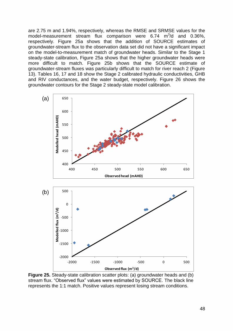
48

are 2.75 m and 1.94%, respectively, whereas the RMSE and SRMSE values for the model-measurement stream flux comparison were 6.74 m3/d and 0.36%, respectively. Figure 25a shows that the addition of SOURCE estimates of groundwater-stream flux to the observation data set did not have a significant impact on the model-to-measurement match of groundwater heads. Similar to the Stage 1 steady-state calibration, Figure 25a shows that the higher groundwater heads were more difficult to match. Figure 25b shows that the SOURCE estimate of groundwater-stream fluxes was particularly difficult to match for river reach 2 (Figure 13). Tables 16, 17 and 18 show the Stage 2 calibrated hydraulic conductivities, GHB and RIV conductances, and the water budget, respectively. Figure 26 shows the groundwater contours for the Stage 2 steady-state model calibration.

Figure 25. Steady-state calibration scatter plots: (a) groundwater heads and (b) stream flux. “Observed flux” values were estimated by SOURCE. The black line represents the 1:1 match. Positive values represent losing stream conditions.

400

450

500

550

600

650

400 450 500 550 600 650

Mo

de

lled

he

ad (

mA

HD

)


-2000

-1500

-1000

-500

0

500

-2000 -1500 -1000 -500 0 500

Mo

de

lled

flu

x (m

3/d

)

Observed flux (m3/d)

(a)

(b)

49

Table 16. Hydraulic conductivities from the Stage 2 steady-state calibration. Aquifer Calibrated K (md-1)

Woolshed Flat Shale 0.182

Aldgate Sandstone 0.200

Stonyfell Quartzite 0.359

Basket Range Sandstone 0.049

Barossa Complex 0.102

Layer 2 1x10-4

Table 17. GHB and RIV conductances from the Stage 2 calibration.

Reach descriptor Calibrated conductance C (m2d -1)

GHB1 0.004

GHB2 2

GHB3 2

GHB4 2

GHB5 2

GHB6 0.005

GHB7 0.002

GHB8 2

GHB9 2

GHB10 2

GHB11 0.001

GHB12 0.002

GHB13 1.7

RIV1 100

RIV2 10

RIV3 100

RIV4 15

RIV5 3

RIV6 4

RIV7 100

Table 18. The water budget for the calibrated steady-state model when taking into account SOURCE estimates of groundwater-stream flux.

Flow source Inflow (GL/year)

Outflow (GL/year)

Net (+ve is inflow) (GL/year)

Recharge 1.9 0.0 1.9

GHB 2.2 0.3 1.9

RIV 0.9 2.1 -1.2

Pumping 0.0 1.2 -1.2

Evapotranspiration 0.0 1.3 -1.3

50

Figure 26. Groundwater contours from the Stage 2 calibrated steady-state model. In addition to the comparison between MODFLOW and SOURCE base flow estimates, other inter-model flux comparisons were undertaken to explore differences between the codes. For example, Figure 27 shows the comparison of surface runoff and recharge between SOURCE and LEACHMG. The comparison between the codes indicates a reasonable match for both runoff and recharge. The annual average recharge from LEACHMG was 115 mm/year, whereas SOURCE produced 143 mm/year. The annual average runoff was 310 mm/year from LEACHMG, and was 368 mm/year for SOURCE.

Head (m AHD)

0 0.5 1 km±

51

Figure 27. Comparison of: (a) surface runoff and (b) recharge between SOURCE and LEACHM.

4.5 Predictions

Four scenarios of future precipitation and potential evapotranspiration have been tested. These were generated from the downscaled climate predictions for the Uraidla weather station, based on the projections of the CNRM CM5 and GFDL ESM2M climate models with the RCP4.5 and RCP8.5 greenhouse gas representative concentration pathways (refer to Section 3.5).

0

100

200

300

400

500

600

700

800

1975 1980 1985 1990 1995 2000 2005

Ru

no

ff (m

m/y

ear

)

Year

LEACHMG

SOURCE

0

50

100

150

200

250

300

1975 1980 1985 1990 1995 2000 2005

Re

char

ge (m

m/y

ear

)

Year

LEACHMG

SOURCE

(a)

(b)

52

For each combination of climate model and RCP, the GIWR project provides 100 realisations of climate variables from 2006 to 2100 for the selected weather station. For each of the four sets of 100 realisations representing a climate model/RCP combination, the total precipitation from 2006 to 2100 in each realisation was summed and the realisation with total rainfall closest to the 50th percentile from the 100 realisations was chosen for testing in the three models (i.e., LEACHM, SOURCE and MODFLOW). Table 19 identifies the realisation number that was selected through this process. The four climate scenarios are referred to as Scenarios 1 to 4 in the following discussion.

Table 19. Climate change predictions applied in this project.

Climate model RCP Realisation Number Scenario

CNRM CM5 4.5 76 1

CNRM CM5 8.5 85 2

GFDL ESM2M 4.5 73 3

GFDL ESM2M 8.5 82 4

It is noteworthy that all four of the selected projection realisations predict lower future precipitation compared to historical observations. For example, the mean annual rainfall in the historical simulations is 1033 mm/year, from the 30 year simulation period, whereas Scenarios 1, 2, 3 and 4 predict mean rainfall values of 1031 mm/year, 1012 mm/year, 1020 mm/year and 956 mm/year, respectively, for the 95-year projection period. Across the four scenarios, predicted rainfall decreased by 0.2–7.5% and reference evapotranspiration increased by 17–20%, relative to historical averages.

4.5.1 LEACHMG Figure 28 shows the average fluxes of recharge, irrigation and runoff from LEACHMG for historical and future climate scenarios. Figure 28 and Table 20 show a decrease in average recharge from 115 mm/year for historical conditions to 64-75 mm/year under predicted future climate scenarios. This represents a decrease of 35–44% in annual recharge. There was a slight increase in runoff, from 310 to 312 mm/year for Scenario 1, and a decrease to 288–306 mm/year for Scenarios 2 to 4. This corresponds to changes in runoff between +1% to -7%. Clearly, LEACHM predicts that recharge is significantly more sensitive than runoff to future climate change impacts.

53

Figure 28. Comparison of historical and future recharge, runoff and irrigation from LEACHM model. Figure 28 indicates that irrigation would increase under future climate conditions, relative to historical usage, from 76 mm/year to 119–129 mm/year for the four scenarios, representing increases of 57-70%. This is a consequence of predicted higher evapotranspiration rates and lower rainfall, leading to more frequent triggering of irrigation to meet vegetation water requirements. The combined influence of enhanced irrigation demand, most likely leading to increased groundwater extraction, and the reduction in recharge rates, may have significant negative impacts on the groundwater resources. A number of assumptions and simplifications need to be highlighted as important factors in interpreting the results offered above. For example: (i) the land use and vegetation types were considered unchanged in future scenarios relative to historical conditions; (ii) the irrigation policies were considered constant in the historical and future scenarios; (iii) vegetation water requirements are met through irrigation, regardless of the state of the groundwater system.

Historical Scenario 1 Scenario 2 Scenario 3 Scenario 40

50

100

150

200

250

300

350R

ech

arg

e,

run

off

an

d irr

iga

tio

n(m

m/y

ea

r)

Recharge scenarios

Recharge

Runoff

Irrigation

54

Table 20. Historical and future recharge, runoff and irrigation simulated by LEACHM.

Scenarios Recharge (mm/year) Runoff (mm/year) Irrigation (mm/year)

Historical 115 310 76

Scenario 1 73 312 119

Scenario 2 70 305 122

Scenario 3 75 306 122

Scenario 4 64 288 129

4.5.2 MODFLOW The calibrated transient model was used for the future projection simulations. The simulation period was extended to account for the 95-year future projections period, otherwise the parameters and settings were kept the same as in the calibrated transient model. This way, the model firstly completes the historical simulation before running one of the four climate scenarios. Each scenario involved different recharge, pumping and potential groundwater evapotranspiration rates. Comparison of water level trends for the four different scenarios is shown in Figure 29. Water balances for the four different scenarios are shown in Tables 21, 22, 23 and 24.

55

Figure 29. Groundwater level hydrographs at observation wells for the four different scenarios. The “Min” and “Max” lines represent minimum and maximum water levels from the calibrated historical hydrographs.

458

460

462

464

466

468

470

472H

ea

d (

mA

HD

)

488

490

492

494

496

498

500

ONK10ONK9

ONK8ONK7

ONK4 ONK6

456

458

460

462

Hea

d (

mA

HD

)

492

494

496

494

496

498

Hea

d (

mA

HD

)

470

472

474

476

478

470

475

480

485

490

Hea

d (

mA

HD

)

Scenario 1

Scenario 2

Scenario 3

Scenario 4

Min

Max

448

450

452

454

456

520

525

530

Hea

d (

mA

HD

)

ONK11 ONK12

ONK14ONK13

ONK15

2010 2020 2030 2040 2050 2060 2070 2080 2090 2100483

484

485

486

Year

2010 2020 2030 2040 2050 2060 2070 2080 2090 2100484

486

488

490

492

Hea

d (

mA

HD

)

Year

56

Table 21. Water balance from Scenario 1. Flow source Total Net Volume Time-Averaged Flux

Recharge 113 GL 1.2 GL/year

GHB 88 GL 926 ML/year

RIV 2 GL 21 ML/year

Pumping -149 GL -1.6 GL/year

Evapotranspiration -55 GL -581 ML/year

Storage change 641 ML 6.7 ML/year

Table 22. Water balance from Scenario 2.

Flow source Total Net Volume Time-Averaged Flux



RIV 6 GL 63 ML/year



Storage change 1 GL 11 ML/year





RIV 1.8 GL 19 ML/year


Evapotranspiration -55 GL 580 ML/year

Storage change 194 ML 2 ML/year





RIV 14 GL 146 ML/year



Storage change 942 ML 9.9 ML/year

57

5. Discussion and Conclusions Individual models of surface water runoff, groundwater recharge and groundwater flow have been developed to assess climate change impacts for the Cox Creek catchment in the Mount Lofty Ranges of South Australia. Key components of the catchment water balance are used to link the three models and provide insights into the combined application of the modelling suite. The results highlight that inconsistencies between the different models can be expected if careful interrogation is not undertaken. For example, internal flux calculations need to be extracted from the models and compared to corresponding processes in complementary models if consistency in the internal fluxes is required across the modelling suite. Some of the key outcomes arising from comparing the three models (LEACHMG, MODFLOW, SOURCE) were:

1. There were mixed outcomes of attempts to extract internal fluxes from the three different hydrological codes. In the case of evapotranspiration rates in SOURCE simulations, these remain largely unknown. Also, subsurface fluxes into and out of the catchment, simulated as boundary inflows/outflows in MODFLOW, are perhaps simulated in SOURCE as otherwise undifferentiated losses, but the modelling team was not able to extract these from SOURCE for comparison to MODFLOW.

2. LEACHMG and SOURCE produce largely consistent predictions of runoff, despite considerable differences in the conceptual structure between the codes.

3. SOURCE and LEACHMG also predicted similar recharge estimates. These are also reasonably consistent with chloride mass balance estimates of recharge.

4. It was possible to reproduce the SOURCE base flow (groundwater discharge to stream) fluxes in the Stage 2 MODFLOW calibration, whereas in the Stage 1 calibration (considering heads only), MODFLOW produced dissimilar base flow fluxes compared to the SOURCE results.

5. It is presently unclear as to the reliability of the SOURCE base flow estimates. The Stage 1 MODFLOW calibration produced groundwater discharge to streams that were significantly smaller than those of SOURCE. Hence, SOURCE estimates of base flow should be validated (e.g., through alternative methods of base flow estimation, such as base flow filters or environmental tracers methods) to determine whether there were inadequate inflows to the aquifer in the Stage 1 calibrated MODFLOW model. The most likely cause of the shortfall in groundwater inflow (i.e. commensurate with the shortfall in the base flow in the Stage 1 calibration model) would be an under-estimation of recharge. However, it is not clear whether MODFLOW or SOURCE is more accurate in their prediction of groundwater discharge to streams, and hence, without further analysis it is not possible to draw conclusive findings regarding this component of the model comparative analysis.

6. The Stage 2 MODFLOW calibration (incorporating SOURCE groundwater discharge to stream fluxes) produced significantly enhanced flows through the model’s boundaries. This was a calibration response to the “shortfall” (relative to SOURCE’s estimates of base flow) in groundwater discharge to streams that was obtained in the Stage 1 calibration, in combination with the fixed (uncalibrated) recharge fluxes that were imposed in the Stage 2 calibration of the MODFLOW model.

58

7. It is somewhat reassuring that the recharge and runoff estimates produced by SOURCE and LEACHM (Figure 27) are largely consistent.

In general terms, all three models were able to reproduce adequate matches to the field observations. Firstly, the MODFLOW model provided a reasonable reproduction of groundwater levels, in terms of both the spatial and temporal water level trends. The lower calibration weighting of single-measurement heads is the reason that these are not as closely matched to the averages from monitoring wells. Secondly, the LEACHM model adequately reproduced both an approximate value for total pumping, and an estimate of recharge obtained from the CMB approach. Thirdly, SOURCE was able to match observed stream flows and gave similar results to LEACHMG. The application of the models to four scenarios of future climate indicates reduced groundwater recharge, enhanced evapotranspiration, largely similar surface runoff, a higher agricultural water demand, and falling groundwater levels. Given that the four climate change scenarios represent lower future precipitation and higher potential evapotranspiration relative to historical conditions, this is somewhat unsurprising. However, the magnitude of future climate change impacts was marked, and considerably larger than the rainfall decline, at least in terms of the recharge reduction. It was surprising that runoff predicted by LEACHMG was largely unchanged under future climate scenarios. In addition to the insights offered above, a number of general lessons learnt regarding the methodology of the current study are apparent in concluding the project. These include:

1. The re-calibration of hydrological models, where several are used in the manner presented in this study, is a necessary element of any study that aims to produce a framework of catchment hydrology simulators with consistent fluxes. Re-calibration requires careful dissection of the various models, and a number of iterations whereby model outputs and internal calculations are compared between codes.

2. For the purposes of producing an optimal model of the Cox Creek aquifers, it is recommended that additional water level measurements are taken from the single-measurement wells that were included in the MODFLOW calibration, to enhance the current understanding of regional groundwater flow in the study area, and to augment the reliability of these measurements.

3. The climate change inputs from GIWR project were of a format that proved to be suitable for input into the various hydrological models of the study area, albeit there needed to be careful selection from the many climate scenarios to allow for a reasonable number of model simulations.

4. The application of three separate models, developed by different organisations brought with it significant challenges in inter-model comparisons and in coordinating the timing of the respective model development activities. The development of a fully integrated catchment hydrology model, capturing the surface systems, soil and groundwater domains would circumvent the considerable effort associated with inter-organisational/inter-model coordination. It may be possible to develop such a model using the WATLAC code developed by the Nanjing Institute of Geography and Limnology (see Zhang and Werner, 2009; Li et al., 2014).

59

There are several areas in which the current work can be extended to produce improved simulation of climate change impacts on the Cox Creek catchment. The key areas of future work include:

1. An improved estimate of base flow is needed, using various hydrologic (e.g. base flow separation filters) and hydrochemical methods (e.g. environmental tracer approaches). This will allow application of the modelling suite to better constrain groundwater recharge.

2. Further investigation of recharge is warranted including closer scrutiny of the chloride mass balance estimates of recharge and their integration into the modelling methodology. For example:

a. The Stage 2 calibration produces rather high values of inflow through the model boundaries, and additional analysis is needed to ascertain whether higher recharge or lower base flow values are required, relative to those produced by LEACHM and SOURCE, respectively.

b. The comparison of LEACHM recharge with CMB recharge neglected the concentration of chloride in groundwater due to direct groundwater evapotranspiration. MODFLOW predicted that groundwater evapotranspiration was significant in the study area, and hence, future revisions to this work should compare the CMB recharge to LEACHM recharge minus the groundwater evapotranspiration predicted by MODFLOW. This would lead to higher recharge estimates using LEACHM than has been used in the current study.

c. The combination of LEACHM’s predictions of soil evapotranspiration, and the evapotranspiration of groundwater in MODFLOW should be compared to available MODIS (Moderate-resolution Imaging Spectroradiometer) estimates of total evapotranspiration, to allow for an independent assessment of catchment evapotranspiration.

d. The CMB approach to estimating recharge needs to account for irrigation and the accompanying chloride loads to the soil and aquifer.

e. An improved application of the CMB method would also be accomplished by a more accurate segregation of stream flow into surface runoff and groundwater discharge, to better account for surface runoffs (in reducing P in the CMB equation), which presently adopt the total stream flow rather than the surface runoff component of stream flow, in modifying the CMB equation to account for surface runoff.

3. An improved characterisation of the geology of the western portion of the study area is warranted to ascertain the extent of the perched aquifer within the Stonyfell Quartzite region, as reported by Stewart and Green (2010). In particular, the high groundwater levels in this area were difficult to match within the MODFLOW calibration, and hence some adaptation of the model to account for aquifer perching in this area may be required

4. Additional effort is required to match aquifer properties to anecdotal evidence regarding the transmissivity of particular geological units. For example, there are some inconsistencies between the calibrated hydraulic conductivities in MODFLOW, as given in Table 16, and the general aquifer yields reported by Banks (2010) and Stewart and Green (2010).

5. Further interrogation of the modelling outputs is needed to determine the respective contributions to base flow in the Cox Creek surface water domain from the different geological provinces of the study area, and whether these

60

are consistent with the respective contributions to stream flow reported by Banks (2010).

6. Finally, as discussed above, the development of a fully integrated surface-subsurface flow model of the study area would be a worthwhile project, and useful comparison to the current undertaking, to offer guidance of the practical application of such models to systems and water management questions considered in the current investigation.

References Alcoe D., Green G., Yan W., 2013. Impacts of Climate Change on Water Resources (ICCWR): Adelaide and Mount Lofty Ranges Natural Resources Management Board Region. DEWNR Technical Report 2013/22, Government of South Australia, through Department of Environment, Water and Natural Resources, Adelaide. Allen R.G., Pereira L.S., Raes D., Smith M., 1998. Crop evapotranspiration: Guidelines for computing crop water requirements. FAO Irrigation and Drainage Paper no. 56. FAO: Rome; 328. Banks E., 2010. Groundwater-surface water interaction in the Cox, Lenswood and Kresbrook Creek Catchments, Western Mount Lofty Ranges, South Australia. DWLBC report 2010/19, Government of South Australia, through Department for Water, Adelaide. Barnett B., Townley L.R., Post V., Evans R.E., Hunt R.J., Peeters L., Richardson S., Werner A.D., Knapton A., Boronkay A., 2012. Australian groundwater modelling guidelines, Waterlines report no. 82, National Water Commission, Canberra, Australia, 203 pp., ISBN: 978-1-921853-91-3, http://archive.nwc.gov.au/library/waterlines/82. Bates B.C., Charles S.P., Hughes J.P., 1998. Stochastic downscaling of numerical climate model simulations. Environmental Modelling & Software, 13 (3-4): 325-331. Carr R., Podger G., 2012. eWater Source — Australia's Next Generation IWRM Modelling Platform, 34th Hydrology and Water Resources Symposium (December 2012), ISBN 978-1-922107-62-6. Charles S.P., Bates B.C., Hughes J.P., 1999a. A spatio-temporal model for downscaling precipitation occurrence and amounts. Journal of Geophysical Research 104 (D24): 31657-31669. Charles S.P., Bates B.C., Whetton P.H., Hughes J.P., 1999b. Validation of downscaling models for changed climate conditions: case study of southwestern Australia. Climate Research 12: 1-14. Charles S.P., Bates B.C., Hughes J.P., 2012. A spatiotemporal model for downscaling precipitation occurrences and amounts. Journal of Geophysical Research Atmospheres 104: 31657–31669.

http://archive.nwc.gov.au/library/waterlines/82

61

Cook P.G., 2003. A guide to regional groundwater flow in fractured rock aquifers. CSIRO Land and Water, 108 pp. Delgado P., Kelley P., Murray N., Satheesh A., 2012. SOURCE User Guide, eWater Cooperative Research Centre, Canberra, Australia. DEWNR, 2014. Dataset of Agreed Climate Change Projections for South Australia. Government of South Australia, though Department of Environment, Water and Natural Resources, Adelaide. DWLBC, 2007. Land and soil spatial data – GIS format. CD-ROM, Government of South Australia, through Department of Water, Land and Biodiversity Conservation, Adelaide. Doherty J., 2005. PEST: Model Independent Parameter Estimation. Edition 5 of user manual. Watermark Numerical computing. Environmental Simulations, Inc., 2010. Guide to using Groundwater Vistas, Version 6. Fleming N.K., Cox J.W., He Y., Thomas S., 2012. Source Catchment hydrological calibration in the Mount Lofty Ranges using PEST parameter optimisation tool. eWater CRC. ISBN: 978-1-921543-63-0. Frost A.J., Charles S.P., Timbal B., Chiew F.H.S., Mehrotra R., Nguyen K.C., Chandler R.E., McGregor J.L., Fu G., Kirono D.G.C., 2011. A comparison of multi-site daily rainfall downscaling techniques under Australian conditions. Journal of Hydrology 408: 1-18. Green G., Banks E., Wilson T., Love A., 2007. Groundwater recharge and flow investigations in the Western Mount Lofty Ranges, South Australia. DWLBC Report 2007/29, Government of South Australia, through Department of Water, Land and Biodiversity Conservation, Adelaide. Harbaugh A.W., Banta E.R., Hill M.C., McDonald M.G., 2000. MODFLOW-2000, the U.S. Geological Survey modular groundwater model user guide to modularisation concepts and groundwater flow process. Denver, CO, Reston, VA: U.S. Geological Survey. Hughes J.P., Guttorp P. Charles S.P., 1999. A non-homogeneous hidden Markov model for precipitation occurrence. Applied Statistics 48 (1): 15-30. Hutson J.L., 2005. Leaching Estimation and Chemistry Model: A process-based model of water and solute movement, transformations, plant uptake and chemical reactions in the unsaturated zone – Model description and user’s guide. New York State College of Agriculture and Life Sciences, Cornell University, Ithaca, New York. Hutson J.L., Cass A., 1987. A retentivity function for use in soil-water simulation models. Journal of Soil Science 38: 105–113.

62

Hutson J.L., Waganet R.J., Niederhofer M.E., 1997. LEACHM, Leaching Estimation and Chemistry Model. A process-based model of water and solute movement, transformations, plant uptake and chemical reactions in the unsaturated zone. Versions LEACHF and LEACHG. Research Series No. R97-1, January 1997. Department of Soil, Crop and Atmospheric Sciences, Cornell University, Ithaca, New York. Hutton J.T., 1976. Chloride in rainwater in relation to distance from the ocean. Search 7:207–208. IPCC, 2013. Climate Change 2013: The physical science basis. Contribution of Working Group I to the Fifth Assessment Report of the Intergovernmental Panel on Climate Change [Stocker T.F., Qin D., Plattner G.K., Tignor M., Allen S.K., Boschung J., Nauels A., Xia Y., Bex V., Midgley P.M., (eds)]. Cambridge University Press, Cambridge, United Kingdom and New York, NY, USA. Kelley P., O’Brien A., 2012. SOURCE Scientific Reference Guide, eWater Cooperative Research Centre, Canberra, Australia. Kirshner S., 2005. Modeling of multivariate time series using hidden Markov models. PhD Thesis, University of California, Irvine, 202 pp. Li Y., Zhang Q., Yao J., Werner A.D., Li X., 2014. Hydrodynamic and hydrological modeling of Poyang Lake-catchment system in China. Journal of Hydrologic Engineering 19(3): 607-616. McDonald M., Harbaugh A., 1988. A modular three-dimensional finite difference groundwater flow model. U.S. Geological Survey,Techniques of Water Resources Investigations, book 6, chapter A1, 586 pp. McMahon T.A., Peel M.C., Lowe L., Srikanthan R., McVicar T.R., 2013. Estimating actual, potential, reference crop and pan evaporation using standard meteorological data: a pragmatic synthesis, Hydrological Earth Systems Science 17: 1331-1363. Morton F.I., 1983. Operational estimates of areal evapotranspiration and their significance to the science and practice of hydrology. Journal of Hydrology 66: 1-76. Moss R., Babiker M., Brinkman S., Calvo E., Carter T., Edmonds J., Elgizouli I., Emori S., Erda L., Hibbard K., Jones R., Kainuma M., Kelleher J., Lamarque JF., Manning M., Matthews B., Meehl J., Zurek M., 2008. Towards New Scenarios for Analysis of Emissions, Climate Change, Impacts, and Response Strategies. Intergovernmental Panel on Climate Change, Geneva. Ordens C.M., Post V.E.A., Werner A.D., Hutson J.L., 2014. Influence of model conceptualisation on one-dimensional recharge quantification: Uley South, South Australia, Hydrogeology Journal 22(4): 795-805. Perrin C., Michel C., Andréassian A., 2003. Improvement of a parsimonious model for streamflow simulation, Journal of Hydrology, 279: 275-289.

63

Preiss W.V., 1993. Neoproterozoic, in Drexel J.F., Preiss W.V., Parker A.J., The geology of South Australia, Vol 1, The Precambrian. South Australia Geological Survey Bulletin, 54, 171-203. Scanlon B.R., Healy R.W., Cook P.G., 2002. Choosing appropriate techniques for quantifying groundwater recharge. Hydrogeology Journal 10: 18–39. Stewart S., Green G., 2010. Groundwater flow model of Cox Creek Catchment, Mount Lofty Ranges, South Australia. DWLBC report 2010/14, Government of South Australia, through Department for Water, Adelaide. Taylor K.E., Stouffer R.J., Meehl G.A., 2012. An Overview of CMIP5 and the Experiment Design. Bulletin of American Meteorological Society, 93: 485–498.

Wood W.W., Sanford W.E., 1995. Chemical and isotopic methods for quantifying groundwater recharge in a regional, semiarid environment. Ground Water 33: 458-468. Zhang Q., Werner A.D.. 2009. Integrated surface-subsurface modeling of Fuxianhu Lake catchment, Southwest China. Water Resources Management 23(11): 2189-2204.

The Goyder Institute for Water Research is a partnership between the South Australian Government through the

Department of Environment, Water and Natural Resources, CSIRO, Flinders University, the University of Adelaide and the University of South Australia.

developing an application test bed for hydrological

Documents