developing a real-time agricultural -...

DEVELOPING A REAL-TIME AGRICULTURAL

DROUGHT MONITORING SYSTEM

FOR DELAWARE

by

Steven M. Quiring

A dissertation submitted to the Faculty of the University of Delaware in partial fulfillment of the requirements for the degree of Doctor of Philosophy in Climatology

Summer 2005

©2005 Steven M. Quiring All Rights Reserved

UMI Number: 3181867

31818672005

UMI MicroformCopyright

All rights reserved. This microform edition is protected against unauthorized copying under Title 17, United States Code.

ProQuest Information and Learning Company 300 North Zeeb Road

P.O. Box 1346 Ann Arbor, MI 48106-1346

by ProQuest Information and Learning Company.

DEVELOPING A REAL-TIME AGRICULTURAL

DROUGHT MONITORING SYSTEM

FOR DELAWARE

by

Steven M. Quiring

Approved: __________________________________________________________ Daniel J. Leathers, Ph.D. Chair of the Department of Geography Approved: __________________________________________________________ Thomas M. Apple, Ph.D. Dean of the College of Arts and Sciences Approved: __________________________________________________________ Conrado M. Gempesaw II, Ph.D. Vice Provost for Academic and International Programs

I certify that I have read this dissertation and that in my opinion it meets the academic and professional standard required by the University as a dissertation for the degree of Doctor of Philosophy.

Signed: __________________________________________________________ David R. Legates, Ph.D. Professor in charge of dissertation I certify that I have read this dissertation and that in my opinion it meets

the academic and professional standard required by the University as a dissertation for the degree of Doctor of Philosophy.

Signed: __________________________________________________________ Tracy L. DeLiberty, Ph.D. Member of dissertation committee I certify that I have read this dissertation and that in my opinion it meets


Signed: __________________________________________________________ Richard T. Field, Ph.D. Member of dissertation committee I certify that I have read this dissertation and that in my opinion it meets


Signed: __________________________________________________________ Daniel J. Leathers, Ph.D. Member of dissertation committee

ACKNOWLEDGMENTS

I feel extremely blessed because during my four years at the University of

Delaware I have worked with many wonderful people. First and foremost, I would

like to acknowledge the friendship (and contributions) of my fellow graduate students.

In particular, I would like to acknowledge two fine officemates, Jonathon Little and

Micah Sklut. I thank them for their friendship and words of wisdom. I would also

like to recognize the members of the ‘hydroclimate research group’ (Kevin Brinson,

Kathy Freeman, and Tianna Bogart). Together we tackled the mysteries of

hydroclimatology and attempted to understand the Enigma (DRL). I would also like

to thank the faculty in the Department of Geography for many stimulating

interactions. The high quality of this program can be directly attributed to the high

quality of the faculty. The contributions of my committee members are also

graciously acknowledged.

I am indebted to Dan Leathers and the Department of Geography for

providing my wife and I with the documentation and support that was required for us

‘foreigners’ to receive the appropriate visas. Without this support, we never would

have had the chance to come to Delaware. Dan also graciously provided me with

constructive feedback on early drafts of several journal articles that I published while

in residence at UD. I would also like to thank Dan for writing numerous letters of

reference.

I have learned a lot from working with David Legates over the last four

years… unfortunately most of it was about NASCAR and the ‘exciting’ world of

iv

politics within the climate change community. Seriously though, David is the main

reason that I chose to pursue my doctoral studies at the University of Delaware.

David has provided me with support and criticism when I needed it and he has given

me time and space to pursue my research interests. I have appreciated the opportunity

to work with David and I am especially grateful for the assistance that he provided

during the job search process. I look forward to continuing to collaborate with him

after I leave Delaware.

Finally and most importantly, I would not be here if it was not for Shona’s

love and support. She willing left her family and friends and moved to another

country so that I could pursue my education. She has taken care of me both

emotionally and financially during my doctoral studies and she is truly deserving of

her PhT (which of course stands for “Putting Hubby Through”).

v

TABLE OF CONTENTS

LIST OF TABLES ........................................................................................................ ix LIST OF FIGURES..................................................................................................... xiv ABSTRACT ...............................................................................................................xvii Chapter 1 INTRODUCTION.............................................................................................. 1 2 DROUGHT AND AGRICULTURAL FORECASTING .................................. 4

2.1 Defining Drought....................................................................................... 4 2.2 Agriculture in Delaware ............................................................................ 4 2.3 The Climate of Delaware........................................................................... 8 2.4 Recent Growing-Season Moisture Variability ........................................ 10 2.5 Factors That Affect Crop Yield............................................................... 14 2.6 Crops and Water Use............................................................................... 18

2.6.1 Corn……..................................................................................... 21 2.7 Climate Monitoring and Climate/Crop Forecasting................................ 24

2.7.1 Importance of Climate Monitoring for Agriculture .................... 24 2.7.2 Existing Climate/Crop Yield Forecasting Products .................... 25 2.7.3 Addressing the Need for Better Monitoring and

Forecasting Tools in Agriculture................................................. 26 3 MODELS OF CROP YIELD ........................................................................... 28

3.1 Crop Yield Modeling............................................................................... 28 3.2 Statistical (Thompson-Type) Crop Models ............................................. 29 3.3 Crop Simulation Models.......................................................................... 32

3.3.1 Description of the DSSAT Crop Models .................................... 36 3.3.2 Description of CERES-Maize ..................................................... 39

3.4 Limitations of Crop Simulation Models.................................................. 40 4 METEOROLOGICAL AND SOIL INPUTS FOR THE CERES-MAIZE

MODEL............................................................................................................ 42 4.1 Meteorological Data ................................................................................ 42 4.2 Solar Radiation Data................................................................................ 48 4.3 Calibrated Radar Precipitation Estimates................................................ 58 4.4 Soils Data................................................................................................. 61

4.4.1 Calculation of the DSSAT Soil Parameters ................................ 63

vi

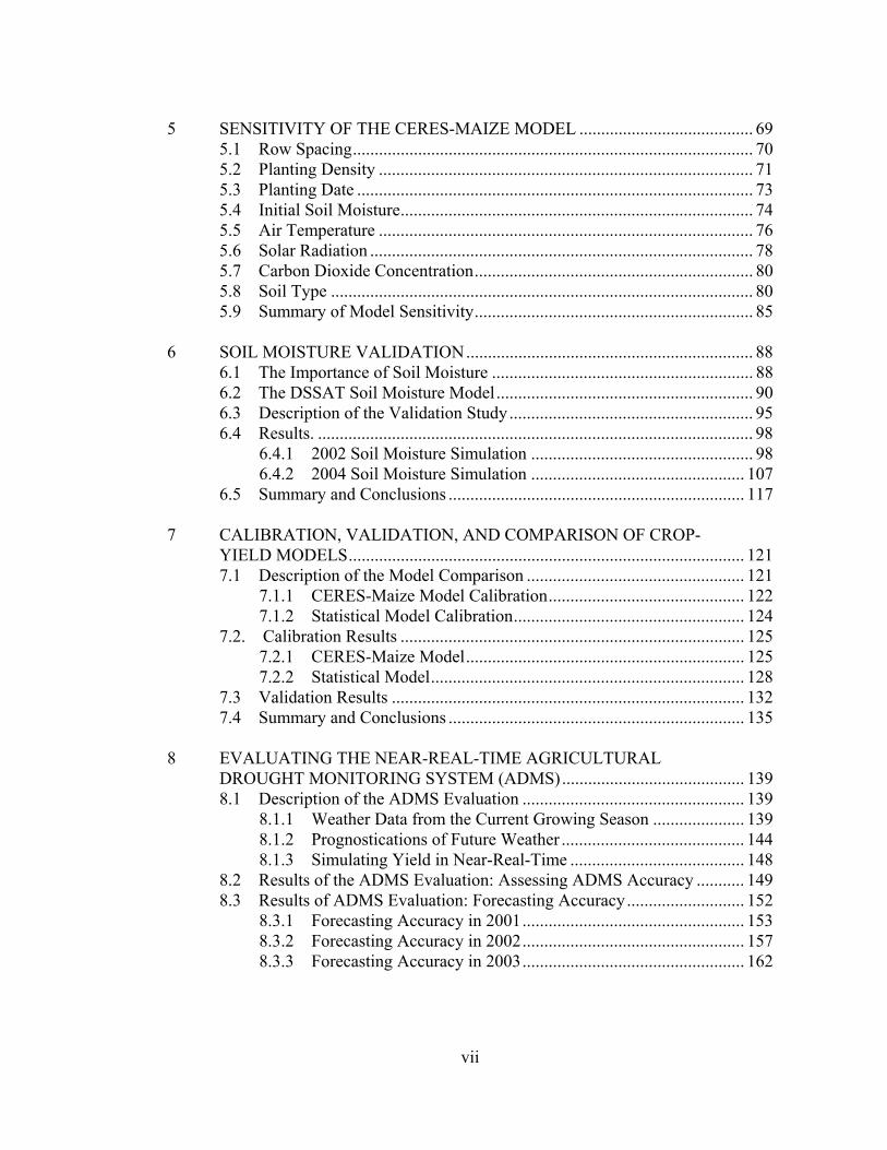
5 SENSITIVITY OF THE CERES-MAIZE MODEL ........................................ 69 5.1 Row Spacing............................................................................................ 70 5.2 Planting Density ...................................................................................... 71 5.3 Planting Date ........................................................................................... 73 5.4 Initial Soil Moisture................................................................................. 74 5.5 Air Temperature ...................................................................................... 76 5.6 Solar Radiation ........................................................................................ 78 5.7 Carbon Dioxide Concentration................................................................ 80 5.8 Soil Type ................................................................................................. 80 5.9 Summary of Model Sensitivity................................................................ 85

6 SOIL MOISTURE VALIDATION.................................................................. 88

6.1 The Importance of Soil Moisture ............................................................ 88 6.2 The DSSAT Soil Moisture Model........................................................... 90 6.3 Description of the Validation Study........................................................ 95 6.4 Results. .................................................................................................... 98

6.4.1 2002 Soil Moisture Simulation ................................................... 98 6.4.2 2004 Soil Moisture Simulation ................................................. 107

6.5 Summary and Conclusions .................................................................... 117 7 CALIBRATION, VALIDATION, AND COMPARISON OF CROP-

YIELD MODELS........................................................................................... 121 7.1 Description of the Model Comparison .................................................. 121

7.1.1 CERES-Maize Model Calibration............................................. 122 7.1.2 Statistical Model Calibration..................................................... 124

7.2. Calibration Results ............................................................................... 125 7.2.1 CERES-Maize Model................................................................ 125 7.2.2 Statistical Model........................................................................ 128

7.3 Validation Results ................................................................................. 132 7.4 Summary and Conclusions .................................................................... 135

8 EVALUATING THE NEAR-REAL-TIME AGRICULTURAL

DROUGHT MONITORING SYSTEM (ADMS).......................................... 139 8.1 Description of the ADMS Evaluation ................................................... 139

8.1.1 Weather Data from the Current Growing Season ..................... 139 8.1.2 Prognostications of Future Weather .......................................... 144 8.1.3 Simulating Yield in Near-Real-Time ........................................ 148

8.2 Results of the ADMS Evaluation: Assessing ADMS Accuracy ........... 149 8.3 Results of ADMS Evaluation: Forecasting Accuracy........................... 152

8.3.1 Forecasting Accuracy in 2001................................................... 153 8.3.2 Forecasting Accuracy in 2002................................................... 157 8.3.3 Forecasting Accuracy in 2003................................................... 162

vii

8.4 Summary and Conclusions .................................................................... 166 9 SUMMARY AND CONCLUSIONS............................................................. 170

9.1 Summary of Results .............................................................................. 170 9.2 Conclusions ........................................................................................... 176 9.3 Future Research ..................................................................................... 177

REFERENCES ........................................................................................................... 180

viii

LIST OF TABLES

Table 2.1: Corn for grain in Delaware (1990–2003) .................................................. 6

Table 2.2: Soybean in Delaware (1990–2003) ........................................................... 6

Table 2.3: Corn for silage in Delaware (1990–2002) ................................................. 7

Table 2.4: Winter wheat in Delaware (1990–2003) ................................................... 7

Table 2.5: Barley in Delaware (1990–2003) .............................................................. 8

Table 2.6: Monthly precipitation (mm) for northern (Climate Division 1) Delaware (1895–2002) .............................................................................. 9

Table 2.7: Monthly precipitation (mm) for southern (Climate Division 2) Delaware (1895–2002) .............................................................................. 9

Table 2.8: Monthly mean air temperature (°C) for northern Delaware – Climate Division 1 (1895–2002) ............................................................. 10

Table 2.9: Monthly mean air temperature (°C) for southern Delaware – Climate Division 2 (1895–2002) ............................................................. 10

Table 2.10 Record and average yields (kg ha-1) and yield losses due to biotic (diseases, insect, and weeds) and physicochemical factors..................... 15

Table 2.11: Growth stages of corn.............................................................................. 22

Table 2.12: Mean dates for corn growth stages based on Georgetown, DE (1984–2003). ........................................................................................... 23

Table 2.13: Decisions farmers make based on climate and weather information ...... 25

Table 3.1: Applications of the DSSAT family of models at different scales ........... 38

Table 4.1: Station history for the COOP station at Georgetown .............................. 43

Table 4.2: Number of days with missing maximum and minimum air temperature and precipitation data at Georgetown.................................. 44

ix

Table 4.3: Station history for the COOP station at Dover........................................ 46

Table 4.4: Number of days with missing maximum and minimum air temperature and precipitation data at Dover ........................................... 46

Table 4.5: Number of days with missing solar radiation data at Georgetown ......... 49

Table 4.6: Calibrated coefficients for the Bristow-Campbell and modified Bristow-Campbell solar radiation models (Goodin et al. 1999) ............. 52

Table 4.7: Comparison of model performance for three solar radiation models: Range of performance statistics across nine evaluation sites in the Northern Great Plains (Mahmood and Hubbard, 2002) ........ 53

Table 4.8: Descriptive statistics of observed and modeled daily solar radiation at Georgetown .......................................................................... 55

Table 4.9: Comparison of model performance for three solar radiation models at Georgetown in 2003.. .......................................................................... 55

Table 4.10: Description of STATSGO soil polygons (MUID) in Delaware.............. 62

Table 4.11: Summary of the main soils used for agriculture in Delaware (STATSGO) ............................................................................................ 63

Table 4.12: Soil color and the associated DSSAT soil albedo ................................... 66

Table 4.13: NRCS drainage classes and the associated DSSAT drainage coefficient ................................................................................................ 66

Table 4.14: SCS runoff curve numbers for cropland.................................................. 67

Table 4.15: Suggested depth of each soil layer in DSSAT soil profile ...................... 67

Table 5.1: Impact of row spacing on yield at Georgetown....................................... 70

Table 5.2: Impact of planting density on yield at Georgetown. ............................... 72

Table 5.3: Impact of planting date on yield at Georgetown. .................................... 75

Table 5.4: Impact of air temperature on yield at Georgetown.................................. 77

Table 5.5: Impact of solar radiation (MJ m-2 day-1) on yield at Georgetown........... 79

Table 5.6: Impact of CO2 concentration (ppm) on yield at Georgetown.................. 81

x

Table 5.7: Characteristics of the ten soils used in the model sensitivity analysis. ................................................................................................... 82

Table 5.8: Impact of soil type on yield at Georgetown ............................................ 84

Table 6.1: Measured versus calculated (estimated) field capacity, wilting point, and available water holding capacity (AWC) at Powder Mill, MD.................................................................................................. 97

Table 6.2: Model performance statistics for the DSSAT soil moisture model at Powder Mill, MD in 2002.................................................................... 99

Table 6.3: Model performance statistics for the first part of the year (January 1 to May 30) at Powder Mill, MD in 2002............................................ 107

Table 6.4: Model performance statistics for the second part of the year (May 31 to December 31) at Powder Mill, MD in 2002................................. 107

Table 6.5: Model performance statistics for the DSSAT soil moisture model at Powder Mill, MD in 2004.................................................................. 108

Table 6.6: Summary of water balance variables at Powder Mill, MD in 2002 and 2004. ............................................................................................... 109

Table 6.7: Model performance statistics for the first part of the year (January 1 to May 29) at Powder Mill, MD in 2004............................................ 112

Table 6.8: Model performance statistics for the second part of the year (May 30 to December 31) at Powder Mill, MD in 2004................................. 112

Table 7.1: Field trial data used for model calibration and model validation.......... 122

Table 7.2: Genetic coefficients for CERES-Maize................................................. 123

Table 7.3: Optimum genetic coefficients for simulating yield at the field trial site in Kent County, Delaware using CERES-Maize. ........................... 125

Table 7.4: Model performance statistics for CERES-Maize during the calibration period................................................................................... 126

Table 7.5: Descriptive statistics for observed yield and CERES-Maize yield predictions (kg ha-1)............................................................................... 126

Table 7.6: Variables in the statistical yield model and their Beta coefficients. ..... 130

xi

Table 7.7: Model performance statistics for the statistical model during the calibration period................................................................................... 131

Table 7.8: Descriptive statistics for observed and statistical model-predicted yield (kg ha-1). ....................................................................................... 131

Table 7.9: Model performance statistics for both yield models (CERES-Maize and statistical) during the validation period. .............................. 134

Table 8.1: Gage-measured and radar-estimated precipitation at Dover (April 1 to October 31, 2001–2003)................................................................. 141

Table 8.2: Gage-measured and radar-estimated precipitation at Wilmington (April 1 to October 31, 2001–2003). ..................................................... 141

Table 8.3: Gage-measured and radar-estimated precipitation at Greenwood (April 1 to October 31, 2002–2003). ..................................................... 141

Table 8.4: Precipitation totals were verified for all days with greater than 76.2 mm (3 in.) of rain (in at least one cell) between April 1 and October 31 (2001–2003)........................................................................ 143

Table 8.5: Number of days with missing maximum and minimum air temperature and precipitation data at Wilmington (1971–2003) .......... 146

Table 8.6: Number of days with missing maximum and minimum air temperature and precipitation data at Dover (1971–1983).................... 147

Table 8.7: Number of days with missing maximum and minimum air temperature and precipitation data at Georgetown (1971–1983).......... 147

Table 8.8: CERES-Maize model parameters used for the ADMS simulations...... 148

Table 8.9: Mean corn production in Delaware by county (2001–2003) ................ 150

Table 8.10: Observed and model-predicted mean corn yield in Delaware (2001–2003) .......................................................................................... 150

Table 8.11: April to October (2001–2003) Standardized Precipitation Index (SPI) values in northern Delaware (Climate Division 1) ...................... 152

Table 8.12: April to October (2001–2003) Standardized Precipitation Index (SPI) values in southern Delaware (Climate Division 2) ...................... 152

xii

Table 8.13: Observed and model-predicted yield for the four forecasting periods in 2001 ...................................................................................... 154

Table 8.14: Observed and model-predicted yield for the four forecasting periods in 2002.. .................................................................................... 159

Table 8.15: Observed and model-predicted yield for the four forecasting periods in 2003.. .................................................................................... 163

xiii

LIST OF FIGURES

Figure 2.1: Monthly precipitation anomalies (January 1997–October 2003) in northern Delaware (Climate Division 1) depicted using monthly and cumulative Standardized Precipitation Index (SPI) values. ............ 11

Figure 2.2: Monthly precipitation anomalies (January 1997–October 2003) in southern Delaware (Climate Division 2) depicted using monthly and cumulative Standardized Precipitation Index (SPI) values. ............ 12

Figure 2.3: Corn (for grain) yield and production in Delaware (1900–2003) .......... 16

Figure 2.4: Soybean yield and production in Delaware (1924–2003)...................... 16

Figure 2.5: Selected corn growth stages. .................................................................. 22

Figure 4.1: Location of meteorological stations used to create weather data set for Georgetown (1984 to 2003). ....................................................... 45

Figure 4.2: Location of meteorological stations used to create weather data set for Little Creek (1984 to 2003)......................................................... 47

Figure 4.3: Scatter plot of measured and modeled (Bristow-Campbell) solar radiation (MJ m-2 day-1) at Georgetown in 2003.................................... 56

Figure 4.4: Measured and modeled daily solar radiation (MJ m-2 day-1) at Georgetown in 2003. .............................................................................. 57

Figure 4.5: Scatter plot of measured and modeled (Mahmood-Hubbard bias adjusted) daily solar radiation (MJ m-2 day-1) at Georgetown in 2003….................................................................................................... 58

Figure 5.1: Seeding density (plants m-2) versus yield (kg ha-1) at Georgetown ....... 72

Figure 5.2: Planting date (month/day) versus yield (kg ha-1) at Georgetown .......... 75

Figure 5.3: Temperature change (°C) versus yield (kg ha-1) at Georgetown............ 78

Figure 6.1: Location of the NRCS SCAN site at Powder Mill, MD ........................ 95

xiv

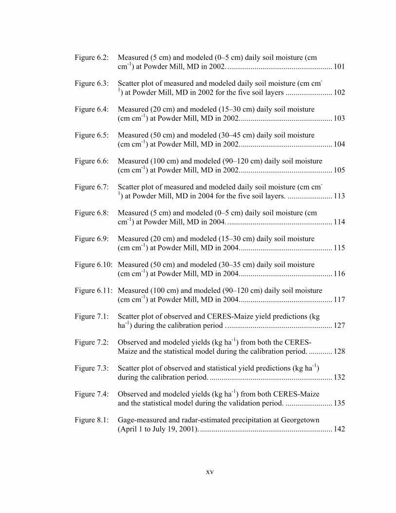
Figure 6.2: Measured (5 cm) and modeled (0–5 cm) daily soil moisture (cm cm-1) at Powder Mill, MD in 2002. ...................................................... 101

Figure 6.3: Scatter plot of measured and modeled daily soil moisture (cm cm-

1) at Powder Mill, MD in 2002 for the five soil layers ........................ 102

Figure 6.4: Measured (20 cm) and modeled (15–30 cm) daily soil moisture (cm cm-1) at Powder Mill, MD in 2002................................................ 103



Figure 6.7: Scatter plot of measured and modeled daily soil moisture (cm cm-

1) at Powder Mill, MD in 2004 for the five soil layers. ....................... 113

Figure 6.8: Measured (5 cm) and modeled (0–5 cm) daily soil moisture (cm cm-1) at Powder Mill, MD in 2004. ...................................................... 114




Figure 7.1: Scatter plot of observed and CERES-Maize yield predictions (kg ha-1) during the calibration period ....................................................... 127

Figure 7.2: Observed and modeled yields (kg ha-1) from both the CERES-Maize and the statistical model during the calibration period. ............ 128

Figure 7.3: Scatter plot of observed and statistical yield predictions (kg ha-1) during the calibration period. ............................................................... 132

Figure 7.4: Observed and modeled yields (kg ha-1) from both CERES-Maize and the statistical model during the validation period. ........................ 135

Figure 8.1: Gage-measured and radar-estimated precipitation at Georgetown (April 1 to July 19, 2001). .................................................................... 142

xv

Figure 8.2: Gage-measured versus bias-adjusted radar-estimated precipitation (mm) .. .................................................................................................. 144

Figure 8.3: Box plots summarizing the yield predictions (kg ha-1) for all 224 grid cells in Delaware for each of the four forecasts: June 1, July 1, August 1, and September and for the observed yield in 2001.......... 156

Figure 8.4: Model-predicted exceedance probabilities (%) for State corn yield based on the June 1, July 1, August 1, and September 1 forecasts in 2001.................................................................................................. 157

Figure 8.5: Box plots summarizing the forecast yield (kg ha-1) for all 224 grid cells for each of the four forecasts (June 1, July 1, August 1, and September 1) and for the observed yield (October 1) in 2002. ............ 160


Figure 8.7: Box plots summarizing the forecast yield (kg ha-1) for all 224 grid cells for each of the four forecasts (June 1, July 1, August 1, and September 1) and for the observed yield (October 1) in 2003. ............ 165


xvi

ABSTRACT

The drought monitoring products currently available are too coarse, both

spatially and temporally, for most agricultural applications. These shortcomings were

addressed by developing a near-real-time Agricultural Drought Monitoring System

(ADMS) for Delaware.

A statistical yield model and a physiological (CERES-Maize) yield model

were calibrated and compared using field trial data from Kent County, DE to

determine which is the most appropriate for predicting corn yield. Although the

statistical yield model was highly correlated with the observed yields during the

calibration period, it did not perform well during the validation period. The results

indicated that statistical models are not appropriate for simulating yield at the field-

level because they are not able to simulate yield during years with extreme weather

conditions and they are location specific.

The sensitivity of the CERES-Maize model was quantified for variations

in row spacing, planting density, planting date, initial soil moisture, carbon dioxide

concentration, air temperature, solar radiation, and soil type. The results indicate that

as row spacing increases and planting density decreases, yields generally decrease.

Increasing the carbon dioxide concentration and solar radiation both resulted in

greater yields. Initial soil moisture (on January 1) does not have a significant impact

on yield. Both air temperature and planting date have a non-linear impact on yield

since they only affect yield during years when precipitation is unequally distributed

xvii

throughout the growing season. Yield is most sensitive to variations in soil type. In

some years, variations in soil type produced yield variations of nearly 300%. The

amount of precipitation and the timing of precipitation in relation to the crop growth

stages determined the magnitude of the soil-type influence. Soil type did not affect

yield when precipitation was abundant and evenly distributed over the growing

season. However, soil type had a major impact on yield during dry years or when

precipitation was distributed such that it was lacking during the moisture sensitive

growth stages.

The soil moisture component of the CERES-Maize model was validated

with observed soil moisture data. The model provides a reasonable approximation of

soil moisture in the upper layers of the soil after May 1. However, there were

significant differences in model performance between 2002 (a drier year) and 2004 (a

wetter year) and the model has difficulties simulating soil moisture in the lowest layer

of the soil and during the first few months of the year. Despite the problems during

the first few months of the year, by the time crops are normally planted (end of April

to beginning of May) the model provides a reasonable simulation of soil moisture in

the upper layers of the soil.

The ability of the ADMS model to accurately simulate State corn yields

using observed weather data was evaluated using three years of data (2001–2003).

After a bias adjustment was applied to the model-predicted State yields, the difference

between the model-predicted and observed state yields varied from 2 to 62 kg ha-1, an

error of less than 1%. It is particularly noteworthy that the model was able to

correctly predict Delaware corn yields during 2001, 2002, and 2003 because growing-

season weather conditions were quite varied.

xviii

The ability of the ADMS to forecast corn yields, from one to four months

prior to harvest, was subsequently assessed by making four forecasts during each

growing season (June 1, July 1, August 1, and September 1) and validating these

forecasts using the results from the full season model simulations. Accurate yield

predictions are difficult to make early in the growing season. In two of the three

years, reasonably accurate yield predictions could be made starting August 1. In all

years, it was possible for the ADMS to accurately predict yields by September 1.

Although this is of little value as a forecasting tool, it does demonstrate that the

ADMS can be used to monitor yields across the state.

Overall, the results suggest that the ADMS provides a useful high-

resolution tool for monitoring soil moisture conditions and predicting crop yield based

on observed weather conditions.

xix

Chapter 1

INTRODUCTION

Agricultural producers, marketing agencies, and the government all

require timely, location-specific soil moisture information -- usually focusing on the

monitoring of drought -- to assist in making operational decisions. The most

advanced (‘state-of-the-art’) drought monitoring product currently available to

decision makers is the United States Drought Monitor (hereafter Drought Monitor),

which was introduced in 1999 (Svoboba et al., 2002). The Drought Monitor was

jointly developed by the National Weather Service (NWS), the National Drought

Mitigation Center (NDMC), and the United States Department of Agriculture’s

(USDA) Joint Agricultural Weather Center. Using a blend of art and science, it

assesses moisture conditions across the United States and provides weekly drought

reports. The Drought Monitor relies on input from a number of different drought and

moisture indices, as well as reports of local conditions. This information is then

synthesized by an ‘expert’ and a preliminary version of the Drought Monitor is

circulated to a panel of federal, state, and academic scientists who can propose

revisions. The Drought Monitor provides a subjective measure of drought conditions

since it is based on a consensus of opinions and a blend of different drought and soil

moisture indices. It is also a highly generalized product, spatially (based on climate

division data), temporally (updated on a weekly basis), and in its focus (accounts for

all types of drought -- meteorological, agricultural, and hydrological).

1

Besides the Drought Monitor, other drought monitoring products are also

produced by the Climate Prediction Center (CPC), the National Climatic Data Center

(NCDC), and the NDMC. These drought monitoring products include national maps

of the Standardized Precipitation Index (SPI), Palmer Drought Severity Index (PDSI),

and modeled soil moisture that are updated on a weekly or monthly basis.

Unfortunately, they have limited utility for agricultural producers and decision makers

because they are difficult to interpret. For example, the method used to calculate these

indices and their meaning is often unclear to non-scientists. They also do not provide

location-specific drought information.

Soil moisture exhibits a great degree of spatial variability because both

soil charactersitics and precipitation are highly variable (Entin et al., 2000). During

the growing season, precipitation inputs can vary greatly over short distances because

much of the precipitation occurs as a result of convective activity. Soil characterstics

(e.g., porosity, water holding capacity, organic content, and texture) also are not

constant, even within a single field. Therefore, the drought monitoring products

currently available are too coarse, both spatially and temporally, for most agricultural

applications. The intention of this dissertation is to address these shortcomings by

developing and validating a methodology (proof-of-concept) for creating a near-real-

time Agricultural Drought Monitoring System (ADMS) for Delaware. Specifically,

the main objectives of this research are to (1) compare (model calibration and

validation) a physiological crop model (CERES-Maize, part of the Decision Support

Systems for Agro-technology Transfer (DSSAT) family of crop-growth models) and a

statistical crop model to determine which is the most appropriate for predicting corn

yield, (2) perform a sensitivity analysis on the crop simulation model (CERES-Maize)

2

to determine how sensitive the model is to uncertainty in the input data, (3) validate

the soil moisture component of the CERES-Maize model, and (4) develop and test the

near-real-time ADMS.

Once it is operational, the ADMS will model soil moisture and provide

crop yield estimates in near-real-time (updated every 24 hours) at a spatial resolution

of 1 arc-minute (approximately 2 km2). The ADMS will provide maps of both crop

yield predictions and current soil moisture conditions. Thus, the introduction of the

ADMS would offer significant improvements over the current suite of available

products by providing high resolution soil moisture and crop yield data to decision

makers. Numerous potential users exist such as agricultural producers, state and

federal agencies, crop insurance companies, agricultural marketing

agencies/commodity boards. It is hoped that this system will provide an effective

means to monitor moisture conditions (agricultural drought) and to make mitigation

and assistance decisions during extreme hydrologic events (floods and droughts).

3

Chapter 2

DROUGHT AND AGRICULTURAL FORECASTING

The purpose of the Agricultural Drought Monitoring System (ADMS) is

to model soil moisture conditions and crop yield across the study region in near-real-

time. Although such systems have been called ‘drought monitoring’ systems, they are

more appropriately termed ‘moisture monitoring’ systems since they are utilized for

all moisture conditions. Although low yields are commonly associated with drought

events, yield is adversely affected by both too much and too little moisture.

2.1 Defining Drought

Drought is a complex phenomenon that is difficult to accurately describe

because its definition is both spatially variant and context dependent. Drought can be

classified into meteorological, agricultural, and hydrological drought (Dracup et al.,

1980). Here, the focus is on agricultural drought, which has been defined as an

interval of time when soil moisture consistently falls below the climatically

appropriate soil moisture such that crop production or range productivity is adversely

affected (adapted from Palmer (1965) and Rosenberg (1978)).

2.2 Agriculture in Delaware

It is estimated that agriculture contributes approximately $1 billion every

year to Delaware’s economy and, although much of this contribution comes from the

4

poultry industry (approximately $619 million), crop production is also important

(Tadesse, 2003). Currently, about 2400 farms in Delaware occupy 560,000 acres

(roughly 45% of the state), of which 480,000 acres are cropland (USDA, 2003). The

two main crops grown in Delaware are corn (Zea mays L.) and soybean (Glycine max

(L.) Merr.). Since 1990, an average of 168,000 acres of corn (Table 2.1) and 216,000

acres of soybeans (Table 2.2) have been planted every year (USDA, 2003) and their

average combined production value is $84 million dollars. It should be noted that

Delaware’s soybean yields includes both production from full season plantings and

production from plantings following the harvest of early season vegetables, barley, or

winter wheat. Those acres that are double-cropped typically account for 40–50% of

the total soybean acreage (Delaware Agricultural Statistics Service, 2003). Other

grain crops grown in Delaware, such as corn for silage (Table 2.3), winter wheat

(Table 2.4), and barley (Table 2.5), are less significant than corn and soybeans

because they occupy fewer acres and have smaller production values. Vegetables are

another important commodity grown in Delaware and, although they occupy a much

smaller amount of farmland than corn and soybeans (only 58,000 acres), they generate

nearly the same amount of revenue since they are a much more valuable crop. Many

different vegetable crops are grown in Delaware and most are extensively irrigated,

making it difficult to model their growth based on meteorological factors alone.

5

Table 2.1: Corn for grain in Delaware (1990–2003)

Year Acres Planted (1000s)

Acres Harvested

(1000s)

Yield (bu/ac)

Production (1000s bu)

Price per Unit ($/bu)

Value of production (1000s of $)

1990 180 172 115.0 19780 2.43 48065 1991 175 169 106.0 17914 2.70 48368 1992 170 161 119.0 19159 2.20 42150 1993 165 160 85.0 13600 2.95 40120 1994 155 150 125.0 18750 2.40 45000 1995 150 144 105.0 15120 3.75 56700 1996 160 154 143.0 22022 3.10 68268 1997 170 160 105.0 16800 2.95 49560 1998 169 155 100.0 15500 2.37 36735 1999 169 154 89.0 13706 2.34 32072 2000 165 155 162.0 25110 2.01 50471 2001 170 162 146.0 23652 2.15 50852 2002 180 167 84.0 13861 2.85 39504 2003 170 160 123.0 20960 --- ---

MEAN 168 159 114.8 18281 2.63 46759

Table 2.2: Soybean in Delaware (1990–2003)


Acres Harvested

(1000s)

Yield (bu/ac)




1990 200 199 34 6766 5.61 37957 1991 255 250 35 8750 5.50 48125 1992 220 215 32 6880 5.50 37840 1993 220 215 23 4945 6.50 32143 1994 225 220 37 8030 5.40 43362 1995 235 233 20 4660 6.95 32387 1996 220 217 35 7595 7.20 54684 1997 230 225 29 6525 7.00 45675 1998 220 216 33 7128 5.31 37850 1999 205 201 27 5427 4.69 25453 2000 215 213 43 9159 4.50 41216 2001 205 201 39 7839 4.25 33316 2002 190 185 25 4625 5.70 26363 2003 180 175 38 6650 --- ---

MEAN 216 212 32 6784 5.70 38182

6

Table 2.3: Corn for silage in Delaware (1990–2002)

Year Acres Harvested

(1000s) Yield (tons) Production

(1000s tons)

1990 7 16 112 1991 5 18 90 1992 8 19 152 1993 4 9 36 1994 4 19 76 1995 5 19 95 1996 5 17 85 1997 9 13 117 1998 10 14 140 1999 10 14 140 2000 9 22 198 2001 7 18 126 2002 10 14 140

MEAN 7 16 116

Table 2.4: Winter wheat in Delaware (1990–2003)


Acres Harvested

(1000s)

Yield (bu/ac)




1990 65 60 51 3060 2.87 8782 1991 70 67 53 3551 2.65 9410 1992 75 70 58 4060 3.10 12586 1993 65 63 57 3591 2.80 10055 1994 75 70 54 3780 3.05 11529 1995 70 68 64 4352 4.10 17843 1996 80 78 53 4134 4.33 17900 1997 75 73 73 5329 3.07 16360 1998 75 73 51 3723 2.35 8749 1999 75 70 57 3990 2.20 8778 2000 65 63 66 4158 2.10 8732 2001 60 57 61 3477 2.45 8519 2002 60 58 70 4060 3.15 12789 2003 50 47 41 1927 --- ---

MEAN 69 66 58 3799 2.94 11695

7

Table 2.5: Barley in Delaware (1990–2003)


Acres Harvested

(1000s)

Yield (bu/ac)




1990 30 27 70 1890 1.89 3572 1991 40 37 68 2516 1.55 3900 1992 40 35 74 2590 1.80 4662 1993 40 35 65 2275 1.60 3640 1994 35 30 63 1890 1.70 3213 1995 40 37 80 2960 1.70 5032 1996 25 23 68 1564 2.98 4661 1997 40 35 89 3115 1.95 6074 1998 34 30 60 1800 1.27 2286 1999 30 26 84 2184 1.35 2948 2000 30 28 81 2268 1.30 2948 2001 29 26 77 2002 1.25 2503 2002 25 23 84 1932 1.40 2705 2003 25 21 59 1239 --- ---

MEAN 33 30 73 2159 1.67 3703

A substantial increase in average crop yields has occurred since the 1950s,

which has been attributed to innovations in farming practices and the introduction of

better yielding varieties (Babb et al., 1997; Michaels, 1983). A portion of this trend

also may be attributed to increasing concentrations of atmospheric CO2 (Idso and Idso,

1994). However, Allen et al. (2003) demonstrated that the small reduction in

evapotranspiration (ET) due to the stomatal closure caused by increasing

concentrations of atmospheric CO2 is more than offset by increases in ET caused by

higher temperatures. Despite the significant enhancement of mean yield over the last

50 years, substantial inter-annual variability remains, most of which can be attributed

to inter-annual variability in growing-season weather conditions.

2.3 The Climate of Delaware

Average annual precipitation ranges from 1070 mm in northern Delaware

(Table 2.6) to 1120 mm in southern Delaware (Table 2.7) and is fairly evenly

8

distributed throughout the year. The wettest months are normally July and August

while February and October/November are usually the driest. Due to the potential

influence of tropical systems, July, August, and September exhibit the most variable

precipitation regimes.

Table 2.6: Monthly precipitation (mm) for northern (Climate Division 1) Delaware (1895–2002)

JAN FEB MAR APR MAY JUN JUL AUG SEP OCT NOV DEC

Mean 83.85 73.68 95.09 88.53 92.31 94.22 107.21 107.15 89.54 77.91 76.80 83.42Median 75.00 69.75 92.62 83.00 90.38 95.62 106.25 89.88 75.12 72.12 68.62 77.12SD 36.50 32.36 39.63 36.13 42.73 39.04 52.89 58.33 50.48 42.24 42.95 40.89Low 15.00 11.50 15.25 17.00 8.50 13.75 10.75 20.50 10.25 5.25 8.25 4.75 High 203.25 164.75 197.00 178.00 198.25 208.75 342.25 305.00 322.75 205.75 189.75 215.75

Table 2.7: Monthly precipitation (mm) for southern (Climate Division 2) Delaware (1895–2002)


Mean 91.72 80.21 102.95 86.22 91.07 90.03 114.16 123.63 95.24 80.72 77.65 86.94Median 83.62 75.75 96.00 85.00 88.12 84.62 100.25 107.75 87.50 71.38 71.50 78.12SD 38.16 34.09 40.90 32.19 45.68 36.64 59.19 71.27 53.11 43.96 40.54 40.00Low 13.00 18.75 34.50 12.75 8.50 23.25 19.75 24.50 1.75 3.00 13.50 13.75High 221.75 166.50 209.75 181.75 296.00 190.75 297.25 367.25 324.75 209.75 187.00 208.00

Mean monthly growing-season air temperatures vary from 17°C in May to

25°C in July (see Tables 2.8 and 2.9). Mean monthly air temperatures always exceed

0°C, although the frost-free period in Wilmington averages 199 days (based on data

from 1894–1998) and the frost-free period in Dover averages 205 days (based on data

from 1948–1999). The last frost normally occurs around the end of April and the first

frost normally occurs at the end of October or the beginning of November (based on

9

the 90% probability). Crop growth in Delaware is affected by the occurrence of

severe weather events such as precipitation extremes, excessive heat, frost, hail, and

severe windstorms; all of which significantly decrease yields.

Table 2.8: Monthly mean air temperature (°C) for northern Delaware – Climate Division 1 (1895–2002)


Mean –0.01 0.48 5.39 10.93 16.79 21.60 24.19 23.28 19.56 13.42 7.36 1.79 Median –0.14 0.72 5.28 10.83 16.67 21.67 24.17 23.28 19.50 13.56 7.28 1.94 SD 2.52 2.49 2.02 1.36 1.34 1.12 0.93 1.08 1.23 1.51 1.45 2.15 Low –6.17 –7.00 0.22 7.72 13.17 18.44 22.06 20.17 16.50 10.28 4.06 –4.11High 6.61 5.11 10.83 14.22 20.44 24.28 26.89 25.61 22.50 16.67 10.83 5.89

Table 2.9: Monthly mean air temperature (°C) for southern Delaware – Climate Division 2 (1895–2002)


Mean 1.56 1.85 6.44 11.43 17.02 21.86 24.47 23.57 20.06 14.05 8.21 3.03 Median 1.44 2.11 6.44 11.17 16.92 21.94 24.39 23.53 19.94 14.22 8.08 3.06 SD 2.58 2.45 2.08 1.37 1.28 1.16 0.93 0.98 1.20 1.48 1.57 2.25 Low –5.00 –4.89 0.28 8.11 13.50 18.33 22.39 20.83 17.28 10.94 4.44 –3.11High 8.22 6.44 12.67 14.44 20.44 25.17 26.72 25.78 23.11 17.33 12.39 7.44

2.4 Recent Growing-Season Moisture Variability

Growing-season moisture variability is one of the main causes of inter-

annual variability in crop yields (Andresen et al., 2001; Purcell et al., 2003). Monthly

precipitation for northern (Figure 2.1) and southern Delaware (Figure 2.2) from

January 1997 to October 2003 has been normalized using the Standardized

Precipitation Index (SPI). In these plots, the greater the precipitation anomaly, the

10

farther the SPI value is from zero. Months that receive greater than (less than) mean

precipitation are assigned a positive (negative) SPI value. The cumulative SPI value

(also shown in Figures 2.1 and 2.2) is a measure of the cumulative severity of a

moisture anomaly and is also used to depict trends in the monthly data.

Figure 2.1: Monthly precipitation anomalies (January 1997–October 2003) in northern Delaware (Climate Division 1) depicted using monthly (bars) and cumulative (line) Standardized Precipitation Index (SPI) values.

11

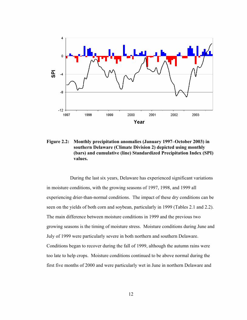
Figure 2.2: Monthly precipitation anomalies (January 1997–October 2003) in southern Delaware (Climate Division 2) depicted using monthly (bars) and cumulative (line) Standardized Precipitation Index (SPI) values.

During the last six years, Delaware has experienced significant variations

in moisture conditions, with the growing seasons of 1997, 1998, and 1999 all

experiencing drier-than-normal conditions. The impact of these dry conditions can be

seen on the yields of both corn and soybean, particularly in 1999 (Tables 2.1 and 2.2).

The main difference between moisture conditions in 1999 and the previous two

growing seasons is the timing of moisture stress. Moisture conditions during June and

July of 1999 were particularly severe in both northern and southern Delaware.

Conditions began to recover during the fall of 1999, although the autumn rains were

too late to help crops. Moisture conditions continued to be above normal during the

first five months of 2000 and were particularly wet in June in northern Delaware and

12

in July in southern Delaware. These moist conditions during the growing season,

combined with a near normal fall, produced record yields for both corn and soybeans

in 2000. Conditions in 2001 were not quite as favorable as 2000 but still resulted in

above average yields.

The extremely dry conditions in October of 2001 signaled the beginning

of a second drought event that persisted into the spring of 2002. Moisture conditions

were near normal in May and June of 2002, but the drier conditions in July ensured

that yields in 2002 would be even less than those during the 1999 drought. Drought

conditions finally abated during the fall and winter as a result of the ample rains that

fell. These wetter-than-normal conditions then continued through much of 2003 and

many places in the Mid-Atlantic received too much rain. Despite the soggy

conditions, corn and soybean yields in 2003 were still above average.

These recent moisture anomalies can be placed in perspective by

examining an 800-year record of growing-season moisture conditions for the southern

Mid-Atlantic that has been reconstructed using tree rings (Stahle et al., 1998). Their

tree-ring chronology is directly correlated with precipitation and inversely correlated

with air temperature, since in the Mid-Atlantic, summer air temperature is not a

limiting factor of growth (Stahle et al., 1998). Careful examination of these

paleoclimatic data reveals that the growing-season moisture anomalies that occurred

during 2002 and 2003 can only be considered rare events if they are evaluated with

respect to the relatively short instrumental record (1895–2003). When these events

are compared to the 800-year reconstructed record, neither is particularly unusual

(Quiring, 2004). The tree-ring data also indicate that growing-season moisture

conditions during the 20th century appear to be well within the range of natural climate

13

variability when compared to the 800-year record (Quiring, 2004). Significant inter-

and intra-annual precipitation variability clearly are normal features of the climate in

Delaware.

2.5 Factors That Affect Crop Yield

Biotic and physicochemical (abiotic) factors affect the quality and

quantity of crop yields (Bushuk, 1982; Kramer and Boyer, 1995; Riha et al., 1996).

Biotic factors include plant diseases, insects, and weeds while the physicochemical

factors include water and nutrient availability, air temperature, daylight, soil pH,

aeration, and the salinity of the soil. Most of the loss in crop yield due to

physicochemical factors can be attributed to soil characteristics. Approximately 45%

of the soils within the United States are classified as permanently dehydrated soils or

shallow soils that are subject to frequent dehydration (Kramer and Boyer, 1995). In

addition, 17% of soils within the United States limit growth because they are too cold,

another 16% of soils are too wet, and 7% of soils have problems with alkalinity or

salinity (Kramer and Boyer, 1995). Only about 12% of soils in the United States are

free of physicochemical problems.

According to Kramer and Boyer (1995), physicochemical factors account

for about a 70% reduction of the maximum potential crop yield and the biotic factors

account for an additional 12% reduction (Table 2.10). Agriculture has addressed this

problem by raising the genetic potential (through the use of hybrids) and by

attempting to change the environment (e.g., fertilizer, irrigation, pesticides). To a

lesser extent, plants also have adapted to the existing environment (Kramer and Boyer,

1995).

14

Table 2.10 Record and average yields (kg ha-1) and yield losses due to biotic (diseases, insect, and weeds) and physicochemical factors. Record yield was measured under conditions that virtually eliminated the pests and competing weeds, and nutrients and water were supplied in ample amounts (it represents potential yield). Average yield was obtained under average conditions (it represents the degree of suppression provided by the environment). Record and average yields are as of 1975.

Crop Record Yield Average Yield Avg. Losses: Diseases

Avg. Losses: Insects

Avg. Losses: Weeds

Avg. Losses: Physico-chemical

Maize 19300 4600 836 836 697 12300 Wheat 14500 1880 387 166 332 11700

Soybean 7390 1610 342 73 415 4950 Sorghum 20100 2830 369 369 533 16000

Oat 10600 1720 623 119 504 7630 Barley 11400 2050 416 149 356 8430 Potato 94100 28200 8370 6170 1322 50000

Sugar beet 121000 42600 10650 7990 5330 54400 Mean % of

record yield

100% 21.5% 5.1% 3.0% 3.5% 66.9%

From: Kramer and Boyer (1995)

Thus, the abiotic factors, especially moisture variability, are the dominant

factors that control yield – up to 80% of the variation in agricultural production can be

attributed to weather variability (Hoogenboom, 2000). This is certainly the case in

Delaware, where recent growing-season droughts during 1999 and 2002 resulted in

significantly reduced yields for corn (Figure 2.3) and soybeans (Figure 2.4). During

these two years, production of corn and soybeans fell to about half of the 2000

production levels. This resulted in nearly $60 million in lost income during these two

years from just corn and soybeans. Absolute correspondence between moisture

conditions and yield is not expected because of other factors that affect yields, such as

damage from pests, disease, weeds, and extreme weather events (Akinremi et al.,

1996a). However, insect infestations and the outbreak of disease are often associated

15

Figure 2.3: Corn (for grain) yield and production in Delaware (1900–2003)

Figure 2.4: Soybean yield and production in Delaware (1924–2003)

16

with drought conditions, which leads to further reductions in yield (Wilhite et al.,

1987).

Temperature is also an important control of crop growth and yield since

the rate of many growth and development processes are controlled by soil or air

temperature (Wheeler et al., 2000). As many development processes (e.g., the rates of

flowering and grain filling) are linear functions of air temperature, when the air

temperature is between some base temperature and an optimum temperature, the

effects of an increase in mean growing-season air temperature can be easily quantified

(Wheeler et al., 2000). Crop simulation studies have shown that increases in mean

seasonal air temperature can result in significant decreases in crop yield, even under

well-watered conditions (Semenov and Porter, 1995). This reduction in yield is due to

shorter crop durations; that is, the crop develops more rapidly at warmer temperatures.

The effects of above normal air temperatures during particularly sensitive

periods of crop growth are of more importance than an increase in the mean growing-

season air temperature. The number of grains in a wheat ear can be substantially

reduced by hot temperatures and low humidity during anthesis (Wheeler et al., 2000).

Increases in air temperature during the late flowering/early pod filling stage of

soybean resulted in a 29% decrease in seed yield (Wheeler et al., 2000). Variability in

air temperature can also affect both yield quality (e.g., wheat protein content)

(Wheeler et al., 2000) and quantity (Semenov and Porter, 1995).

Quality of the soil is another factor that influences yield quality and

quantity. Crops remove nitrogen, potassium, calcium, phosphorus, and micronutrients

from the soil as they grow (Bushuk, 1982). Crops grown on more fertile, well-drained

soils will produce higher yields than those crops grown on less fertile, poorly-drained

17

soils. Soil characteristics not only vary across the State, but even within a single farm

field.

Despite advances in biological engineering, and insecticide and fungicide

treatments, crops continue to be adversely affected by insects and disease (Bushuk,

1982). Probably the most problematic insect in Delaware is the soybean cyst

nematode (CSN), a microscopic parasitic worm (Taylor, 1998). A large percentage of

the acreage in southern Delaware is infected with this pest and these organisms can

cause substantial yield losses. Crop rotation or by planting CSN-resistant varieties of

soybean is the only way these pests can be managed. Weeds also reduce yield

quantity and quality because they rob crops of moisture and nutrients. Therefore,

weed control also is an essential feature of water conservation.

2.6 Crops and Water Use

Water supply is the most significant factor in determining the spatial

distribution of plant species over the earth (Bouten, 1995). Plants need an enormous

amount of water – up to one thousand times as much as their biomass production

(Bouten, 1995). A typical grassland/crop requires about 500 kg of water for

transpiration to produce 1 kg of dry matter (Volkmar and Woodbury, 1995) and a

single corn plant uses more than 200 liters of water (about 100 times its fresh weight)

during its lifetime (Srivastava and Kumar, 1995).

Water-use efficiency (WUE) can be defined as the total dry matter

production (crop yield) per unit of water used in evapotranspiration (Eastin and

Sullivan, 1984). A direct linear relationship exists between water use

(evapotranspiration) and dry matter production (plant growth). WUE varies by plant

species, location, on both an inter- and intra-annual basis (Kramer and Boyer, 1995;

18

Purcell et al., 2003). These differences occur because WUE is primarily driven by the

evaporative demand (vapor pressure gradient). Although agronomic practices can

influence transpiration, they have little impact on WUE. This was demonstrated by

Specht et al. (2001) where despite the application of various agronomic treatments

(e.g., planting dates, soil treatments) at a given site, all of the data points fell along a

single yield-to-water regression line, thus indicating a common WUE.

Plants can be divided into three categories based on how efficiently they

use water during photosynthesis. The majority of plants grown in temperate climates

utilize C3 photosynthesis. C3 plants ‘fix’ CO2 using the Calvin cycle, the process

whereby energy from light reactions (photosynthesis) is used to convert (‘fix’)

gaseous CO2 into sugars. The byproducts of photosynthesis, water vapor and oxygen,

are released through the stomates. When it is hot and dry, C3 plants keep their

stomata closed to prevent water loss, but this also reduces the intake of CO2, carbon

fixation, and plant growth. C3 plants such as barley, wheat, and alfalfa have a WUE

of 2 to 3 g kg-1 (Kramer and Boyer, 1995).

On the other hand, C4 photosynthesis avoids the reductions caused by

photorespiration by separating the initial fixation of CO2 (outer cells) from the Calvin

cycle (inner cells). Since the C4 pathway requires the expenditure of additional

energy, it is only more efficient than C3 photosynthesis when conditions are hot and

dry. C4 plants such as corn, sorghum, and millet have a higher rate of photosynthesis

per unit of water than C3 plants (WUE of between 3 to 5 g kg-1). CAM (Crassulacean

Acid Metabolism) is another type of C4 photoshythesis where the initial carbon

fixation and the Calvin cycle are separated in time. In CAM plants, CO2 enters the

leaf and initial carbon fixation occurs only at night, thus limiting water loss. During

19

the day, light is used to drive photosynthesis and the Calvin cycle (C3

photosynthesis). CAM photosynthesis conserves water better than even C4

photosynthesis, but plants fix relatively little carbon and therefore grow slowly. CAM

plants, such as pineapple, have a WUE of about 20 g kg-1 and are primarily grown in

arid regions (Chaves et al., 2003).

The difference between the amount of water a crop can potentially use

(the crop water demand) and the amount it actually receives during the growing

season is the crop moisture stress. The amount of water available to a crop in any

given year is determined by the amount and distribution of rainfall, the horizontal

transport of moisture, the rate of evaporation, the water holding capacity of the soil,

and the amount of soil moisture at planting (Bouten, 1995). Crop moisture stress

reduces crop yields by three main mechanisms. First, moisture stress may cause a

reduction in the amount of photosynthetically active radiation (PAR) that is absorbed

by the canopy (Earl and Davis, 2003). This occurs as a result of leaf wilting or

rolling, reduced leaf area expansion, and early leaf senescence (Earl and Davis, 2003).

Secondly, moisture stress can reduce the efficiency by which absorbed PAR is used by

the plant (e.g., a reduction in radiation use efficiency (RUE)). Third, moisture stress

may limit the grain yield, especially if it occurs during a critical stage of development

(Earl and Davis, 2003).

The changing water demands of the plant during each growth stage also

are important to accurately predict yield (Wilhite et al., 1987). If a crop yield model is

employed without regard to developmental sensitivity, its ability to predict yield will

be severely limited. For example, if drought occurs when the crop’s water demand is

20

relatively small, there may be little negative impact on the crop. Therefore, the timing

of precipitation is just as important as the total amount of precipitation that occurs.

However, too much precipitation can be just as detrimental to crops as too

little. Waterlogging is a problem, especially in heavy soils, because of the importance

of soil aeration. If excess precipitation falls just prior to planting, seedlings may not

establish deep root systems, making them more susceptible to moisture stress later in

the growing season. If soybean becomes waterlogged for as little as two days, yield

can be reduced, depending on the growth stage, from 18% to 26% (Sullivan et al.,

2001). If flooded conditions persist for longer than two days, yield losses will

increase. Excessive precipitation during harvest is also detrimental because it can

reduce the quality and quantity of yield.

2.6.1 Corn

Table 2.11 and Figure 2.5 outline the growth stages of corn. In Delaware,

corn is typically planted toward the end of April and harvested near the middle to the

end of September (Table 2.12).

Corn is most susceptible to water deficit during tasseling (VT) and silking

(R1), when the aerial transfer of pollen from tassels to silks occurs (Kramer and

Boyer, 1995). The harvest index, the ratio of the economic yield (i.e., the mass of that

part of the plant with economic value) to the biological yield (i.e., the total dry matter

production), is significantly reduced by drought during the filling stage (R2–R5)

(Araus et al., 2002; Roygard et al., 2002). The early stages of reproduction are more

susceptible to water stress than any other stage of development because the corn plant

requires the most water and without pollination, no grain is produced.

21

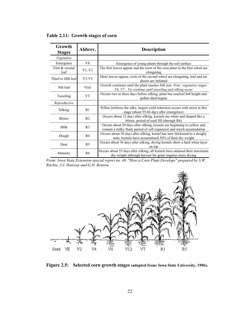
Table 2.11: Growth stages of corn

Growth Stages Abbrev. Description

Vegetative Emergence VE Emergence of young plants through the soil surface

First & second leaf V1, V2 The first leaves appear and the roots of the corn plant in the first whorl are

elongating

Third to fifth leaf V3-V5 More leaves appear, roots of the second whorl are elongating, leaf and ear shoots are initiated

Nth leaf V(n) Growth continues until the plant reaches full size. Note: vegetative stages V6, V7... Vn continue until tasseling and silking occur

Tasseling VT Occurs two or three days before silking, plant has reached full height and pollen shed begins

Reproductive

Silking R1 Pollen fertilizes the silks, largest yield reduction occurs with stress at this stage (about 55-66 days after emergence)

Blister R2 Occurs about 12 days after silking, kernels are white and shaped like a blister, period of seed fill (through R6)

Milk R3 Occurs about 20 days after silking, kernels are beginning to yellow and contain a milky fluid, period of cell expansion and starch accumulation

Dough R4 Occurs about 26 days after silking, kernel has now thickened to a doughy state, kernels have accumulated 50% of their dry weight

Dent R5 Occurs about 36 days after silking, drying kernels show a hard white layer on top

Maturity R6 Occurs about 55 days after silking, all kernels have attained their maximum dry weight although harvest for grain requires more drying

From: Iowa State Extension special report no. 48, "How a Corn Plant Develops" prepared by S.W. Ritchie, J.J. Hanway and G.O. Benson.

Figure 2.5: Selected corn growth stages (adapted from: Iowa State University, 1996).

22

Table 2.12: Mean dates for corn growth stages based on Georgetown, DE (1984–2003). Planting and harvest dates are based on field-trial results from the Research and Education Center (REC) in Georgetown and the dates for the other growth stages were determined from model simulations (CERES-Maize).

Growth Stage Mean Date

Planting April 23 Emergence May 5

End of juvenile May 24 Floral initiation May 29

75% silking July 2 Start of grain fill July 13 End of grain fill August 18

Maturity August 20 Harvest September 18

Sensitivity of a corn plant to drought during pollination is caused by the

physical separation of male and female flowers on the plant. The male flowers are

borne on the tassel and its sole purpose is to produce adequate amounts of pollen.

Pollen shed usually occurs for five to eight days, with peak production occurring on

the third day. A typical tassel will produce two to five million pollen grains, so pollen

shortage is normally not a problem, except for conditions of extreme heat or a nutrient

deficiency, when silk emergence coincides with pollen shed (Vasilas and Tayor,

1998). The silks, the pollen receptor sites, normally start to emerge one to two days

after pollen shed begins. Under optimum conditions, all of the silks will emerge

within three days, providing enough time for all silks to be pollinated before pollen

shed stops. Although a number of pollen grains may attach to each silk, only one

pollen grain will fertilize each ovule (potential kernel) on the ear (arrangement of

female flowers each ending in a silk).

Drought stress can disrupt pollination in a number of ways. High

temperatures can kill the tassel so that no viable pollen is shed, or they can kill the

23

pollen after it is shed (Vasilas and Tayor, 1998). Drought stress can also dry out the

silks. Each pollen grain draws moisture from the silk and the pollen will not

germinate if the silks are too dry (Vasilas and Tayor, 1998). The most frequent way

that drought reduces pollination is by disrupting the synchronization of the pollen shed

and silk emergence. Tassel and pollen formation take priority over silk and ear

formation, therefore drought stress prior to tasseling will delay silk emergence and by

the time the silks emerge pollen shed may have ended (Vasilas and Tayor, 1998).

Even relatively short periods of water stress (6 to 8 days) during tasseling and

pollination can reduce yields by 50% (Roygard et al., 2002).

Water is the main limiting factor to rainfed corn in the Mid-Atlantic

coastal plain (Roygard et al., 2002). Rainfed corn lacks the drought tolerance required

to produce reliable yields year after year. The sandy soils of southern Delaware will

not support a crop rotation of corn and soybean unless additional water is supplied by

irrigation (Taylor, 1998). Soils with a high water-holding capacity help minimize

water stress during the critical growth phases (Roygard et al., 2002). In addition, corn

plants stressed from excessive populations, inadequate fertility, or disease infection

also use water less efficiently and produce lower yields.

2.7 Climate Monitoring and Climate/Crop Forecasting

2.7.1 Importance of Climate Monitoring for Agriculture

Climate has both direct and indirect effects on agriculture through, for

example, soil and vegetation, nutrient loss, water availability, pests and diseases, land

use practices, marketing, and transportation (Ogallo et al., 2000). Interannual climate

variability and, in particular, extreme events can have a devastating impact on

24

agriculture (Ogallo et al., 2000). In agri-business, weather risk is viewed as the

uncertainty created in earnings due to weather variability (Wilhelmi et al., 2002).

Thus, many of the decisions made by agricultural producers are determined by current

agrometeorological conditions. For example, knowledge of current soil moisture

conditions is used to assess the length of the rainfed cropping season and to make

decisions regarding many agricultural activities (Table 2.13) such as accessibility of

the fields, land preparation, sowing, germination, weeding, thinning, supplemental

irrigation (irrigation scheduling), harvesting and post-harvesting operations like

drying and storage (Rijks and Baradas, 2000). Information on current moisture

conditions can also be used as input for disease and pest models and to increase water

use efficiency.

Table 2.13: Decisions farmers make based on climate and weather information

Climate Weather

Choice of farming system Timing, land preparation, land layout

Choice of crops Date of planting

Choice of optimal variety Choice of alternative variety

Choice of farm equipment Actual daily use of farm equipment

Choice of row width Within-row distance of plants

Choice of irrigation Timing and amount of water applied

Choice of pest control system Timing and extent of controls

Adapted from: Rijks and Baradas (2000)

2.7.2 Existing Climate/Crop Yield Forecasting Products

Agricultural forecast models and predictions are often based on global

teleconnection patterns such as ENSO (Everingham et al., 2003; Meinke and Hammer,

1997; Meinke et al., 1996; Stone and Auliciems, 1992; Stone et al., 1996a; Stone et

25

al., 1996b). These forecasts rely upon known associations between the phase of

ENSO and climatic conditions in various regions around the world and have proven to

be particularly accurate during strong ENSO events. Most seasonal forecasting skill

lies in the tropics and subtropics while forecasts are less skillful at higher latitudes in

the Northern Hemisphere. Nonetheless, operational seasonal forecasts are produced

by a number of centers, including the Hadley Center, the CPC, the European Center

for Medium-Range Weather Forecasts (ECMWF), and the International Research

Institute for Climate Prediction (IRI). However, many of their products are still

considered experimental because their forecasts lack certainty, particularly in terms of

forecasting growing-season precipitation in the mid-latitudes. While these seasonal-

forecast models are continually improved, much work remains before they can be

considered useful to agricultural producers (Quiring and Papakyriakou, 2005). These

advances offer the opportunity to reduce the risk associated with climate variability.

2.7.3 Addressing the Need for Better Monitoring and Forecasting Tools in Agriculture

Climate monitoring information and crop forecasts must be both timely

and appropriate to be helpful in making operational and planning decisions in

agriculture (Weiss et al., 2000). User-specific weather information for planning,

adaptation of systems, and daily operations involving the dosage and timing of inputs

can have a major effect on production (Rijks and Baradas, 2000). While agricultural

operations require real-time or near-real-time agrometeorological information, this

information is difficult to provide because land-use activities and soil characteristics

can vary greatly, even over short distances. In addition, most observation networks

are not of sufficient spatial density (resolution) to provide accurate information. One

26

important advance is the incorporation of remotely-sensed data to provide near-real-

time agrometeorological information. Although this technology can provide complete

spatial coverage, the resolution is often too coarse to provide farm-level data.

Remote-sensing techniques, hold the key to future applications and advances in

providing real-time data for operational and planning decisions (Ogallo et al., 2000).

Considerable potential exists for adjusting crop management if climate

monitoring and forecasting systems can be improved, but the complexities of

agricultural systems and the uncertainties of climate forecasts suggest that more

research is required before this becomes a reality (Jones et al., 2000). Improving

agrometeorological monitoring and forecasting will require better observation

networks (increased station density, real-time observations, and more reliable data),

the development of agriculture-specific monitoring and forecasting products, and the

development of an integrated agrometeorological information system to facilitate

timely decision making (Ogallo et al., 2000). Commodity forecasts are becoming

increasingly utilized in agricultural industries to improve risk management and

decision-making at the regional scale (Potgieter et al., 2003). A regional commodity

forecasting system incorporates crop-specific modeling with actual climate up to the

forecast data and projects crop conditions given likely future climate scenarios.

27

Chapter 3

MODELS OF CROP YIELD

3.1 Crop Yield Modeling

The Agricultural Drought Monitoring System (ADMS) will provide near-

real-time predictions of crop yield based on the observed growing-season air

temperature and precipitation. Although numerous models have been developed to

predict crop yield, most can be described as deterministic because, given a particular

set of conditions, they calculate a single yield prediction (Hoogenboom, 2000).

Ritchie (1994) identified three types of deterministic models – namely, statistical

models, mechanistic models, and functional models. Statistical models are used to

make yield predictions (typically over a large area) based on weather variables. The

purpose of mechanistic models is to replicate all of the plant growth and development

processes for a single plant using mathematical equations. Since mechanistic models

are not appropriate for regional-scale predictions of yield, they will not be discussed

here. Functional models use simplified mathematical and/or empirical equations to

represent the relationships between environmental conditions and plant growth and

development processes. Functional crop models can also be described as simulation

or physiologically-based models because they use one or more sets of differential

equations to calculate rate and state variables over time (normally from planting until

harvest) and to express the relationships between plant growth and environmental

28

conditions. This is in contrast to statistical models, which are based simply on

correlations between crop yield and some surrogate variable, usually weather related.

3.2 Statistical (Thompson-Type) Crop Models

One of the simplest methods for predicting crop yield is to use regression

techniques to relate weather variables to crop yield (Duchon, 1986). This approach

attempts to create a model that simulates yield given the current and past weather

conditions during the growing season. These statistical crop-yield models are often

called Thompson-type models, after the work of Thompson (1969; 1970; 1975).

Thompson elaborated on the pioneering work carried out by Wallace (1920) to

develop statistical models for grain yield based on environmental variables such as

monthly air temperature and precipitation.

More recently, Michaels used Thompson-type yield models to examine

the climatic sensitivity of high yielding varieties of wheat (Michaels, 1982) and to

study the economic and climatic factors associated with acreage abandonment

(Michaels, 1983; Michaels, 1985). The statistical model used by Michaels (1983) to

explain acreage abandonment of winter wheat in the United States Great Plains, which

included price and weather variables, accounted for 77% of the variance in

abandonment. Subsequently, Michaels (1985) performed a similar analysis of acreage

abandonment for spring wheat in a series of crop reporting districts in North and

South Dakota and Minnesota. That statistical model was able to explain 60% of the

variance in acreage abandonment, the majority of which was related to weather

variability (53%). Price variables (e.g., Chicago Board of Trade future price quotes)

were statistically significant, but of minor importance, in comparison to weather

variability.

29

Michaels (1985) employed two tests to verify model reliability. In the

first test, successive three-year blocks of data were withheld from the model and then

predicted using the new regression parameters. The model was able to explain about

45% of the variance in acreage abandonment for those withheld years in this test. In

the second test, the first 10 years of model input were withheld, and abandonment

during those years was predicted from the remaining data. Only 11% of the variation

was explained using this test, however. The poor performance of the second test is not

surprising given the unprecedented acreage abandonment during this 10-year block

(1932–1941). Therefore, Michaels (1985) concluded that the true model accuracy

likely falls somewhere between 11–45%. Michaels’ findings highlight one of the

main weakness of the Thompson-type yield models –– their inability to successfully

model extreme or unusual climatic events (Michaels, 1983).

Predominantly, Thompson-type models use air temperature, precipitation,

and evapotranspiration (Babb et al., 1997; McGregor, 1993; Quiring and Blair, 2000)

to model yield. Such models tend to be most accurate in regions where moisture is a

major limiting factor of crop growth. Because of the importance of ET in determining

crop yield (Arora et al., 1987), subsequent researchers have turned to Palmer’s Z-

index (Palmer, 1965), instead of air temperature and precipitation data, to predict yield

deviations of corn (Sakamoto, 1978) and spring wheat (Quiring and Papakyriakou,

2003). In addition to weather conditions, the impact of improvements in agricultural

technology is also an important variable included in most statistical yield models

(McGregor, 1993). Overall, Thompson-Type models are the simplest models to

employ because of their limited data requirements. However, they are not easily

30

transferable to different locations because the regression coefficients are location- and

time-period specific.

Thompson-type crop yield models are usually calculated using climatic

data from a large number of subregions (e.g., crop reporting districts from a number of

states). Data from all regions are pooled and constant and trend values are

simultaneously calculated for each subregion (e.g., individual crop reporting districts).

This increases the number of degrees of freedom in the model by taking advantage of

the spatial differences in observed weather and crop yields. The general form of the

model for a regional estimate is given by

Ŷ = Yb + Yt + Yc + ε I (3.1)

where Ŷ is the yield estimate, Yb is a constant generated for each crop district, related

to the mean yields at the beginning of the time series (e.g., soil conditions), Yt is a

variable related to the increase in yields due to technological trends, Yc is a variable

related to the effect of climatic variability on yield, and εi is the unexplained residual,

distributed as NID(0, σ2). The constant for each crop district, Yb, is computed from

Yb = Σ BjKj (3.2)

where Yb is the product of a dummy variable, Kj, and a least-squares regression

coefficient, Bj. Here, Kj is unity for the jth crop district and is zero for all other crop

districts. The constant, Yb, represents an objectively derived indicator of yield at the

beginning of each time series while the other variables are held constant (e.g., average

climate conditions and no time-related increases in yield). It also measures the

spatially varying component of base yields and is controlled by factors other than

technology and climate that have a spatial component, such as soil type, and elevation.

The technological trend variable, Yt, is

31

Yt = Σ CjTj (3.3)

where Yt is the product of a dummy variable, Tj, and a least-squares regression

coefficient, Cj. By convention, Tj is zero for all crop districts prior to 1945 and then

increases by one for each subsequent year. This variable accounts for the observed

increase in yield over time that can be attributed to technological innovations.

The effect of climatic variability on yield, Yc, for an individual crop

district is

( ) ( ) ( ) ( )

( ) ( )∑=

−−+

−′+−′+−+−=

n

iiii

iiiiiiiic

PPTT

PPTTPPTTY

11010

21010

21010

loglog

loglogloglog

λ

βαβα (3.4)

where Yc is a function of the observed monthly mean air temperature (Ti), precipitation

(Pi), and interaction between air temperature and precipitation. Air temperatures are

expressed as departures from the grand mean, T (averaged over all crop districts and

months). Precipitation is also expressed as a departure from the large area mean, P .

The log transformation of precipitation allows for the growth response from a small

increase in precipitation under drought conditions to be greater than the growth

response under a similar increase in precipitation when there is abundant moisture

(non-linear response of yield to moisture supply). This also limits the impact of large

amounts of precipitation from convective events. Both air temperature and

precipitation are also expressed as squared terms to allow for the determination of

optimal yield response.

3.3 Crop Simulation Models

Like Thompson-Type models, crop simulation models are useful tools for

determining the impact of growing-season moisture variations on plant growth and

yield (Ewert et al., 2002). Most crop simulation (or physiologically-based) models

32

examine temporal variations in crop growth using site-specific data and, therefore, the

outputs from such models are also site-specific. Crop simulation models have been

used extensively to model crop yields based on weather conditions at a variety of

scales from the field level to the national level (Hoogenboom, 2000).

Management applications serve as one of the main uses of crop simulation

models and these can be strategic, tactical, or forecasting. Strategic applications of

crop simulation models are employed prior to the growing season to evaluate

alternative management strategies (e.g., to evaluate ‘what-if’ scenarios regarding crop

rotation, cultivar, plant density, and row spacing) (Anapalli et al., 2005). This can

help farmers reduce inputs and increase returns (increase productivity). Tactical

applications are employed both before and during the growing season to allow the

farmer to make management decisions based on the growing season weather to date

(e.g., timing and amount of fertilizer and irrigation applications). Forecasting

applications can be conducted either prior to planting or during the growing season

and are used to make marketing decisions or by the government to make policy

decisions (Bannayan et al., 2003; Chipanshi et al., 1997; Guérif and Duke, 2000;

Hoogenboom, 2000; Jagtap and Jones, 2002). Crop simulation models can be

effectively used for crop prediction applications if accurate weather information is

available both with respect to observed and forecast conditions (Hoogenboom, 2000).

Stochastic modeling can also be used with forecasting applications to determine the

probability distribution of yields and therefore the risks associated with certain

management decisions.

Crop simulation models also have been used in a variety of research

applications such as analyzing the impact of climate change and climate variability on

33

agriculture (Andresen et al., 2001; Attri and Rathore, 2003; Carbone et al., 2003;

Easterling et al., 1993; Ewert et al., 2002; Keating and Meinke, 1998; Mearns, 1983;

Semenov and Porter, 1995; Southworth et al., 2002; Tubiello et al., 2002; Xie et al.,

2001). Crop models have even been used to identify opportunities for genetic

improvement (Boote et al., 2003). All of these applications can provide information

to facilitate decision making by the farmer, policy maker, or other agricultural

decision maker.

As a large number of crop simulation models have been developed, it is

useful to divide them into logical groups. Penning de Vries et al. (1989) classified

crop simulation models based on the level of detail that they use to characterize the

relationships between environmental conditions and crop growth. Level 1 models use

only air temperature and solar radiation to simulate crop growth and development.

These models determine yield just by simulating the plant carbon balance. Level 2

models require precipitation and irrigation data in addition to the data required for

level 1 models. Level 2 models simulate the soil and plant water balances in addition

to the carbon balance. Level 3 models are more complex than level 2 models because

they require soil nitrogen input data and they calculate the soil and plant nitrogen

balance. Level 4 models require data on other soil minerals as well as data on pests,

diseases, and weeds. These models simulate the complete soil-plant-atmosphere

system. Very few crop models have reached level 4. Most of the commonly used

crop simulation models such as the Erosion Productivity Impact Calculator (EPIC)

(Easterling et al., 1993), the Root Zone Water Quality Model (RZWQM) (Nielsen et

al., 2002), Agricultural Land Management Alternatives with Numerical Assessment

(ALMANAC) (Xie et al., 2001), Sorghum Kansas A&M (SORKAM) (Xie et al.,

34

2001), AFRCWHEAT2 (Ewert et al., 2002), SUCROS (Guérif and Duke, 2000), the

Agricultural Production Systems Simulator (APSIM) (Keating and Meinke, 1998),

LINTULCC2 (Ewert et al., 2002), Sirius (Ewert et al., 2002), the Crop-Environment

Resource System (CERES) (Tsuji et al., 1994), and CROPGRO (Tsuji et al., 1994) are

level 3 models. These models simulate crop growth and development and the carbon,

soil/plant water, and nitrogen balances. The last two models, CERES and CROPGRO,

are both part of the Decision Support System for Agrotechnology Transfer (DSSAT)

family of crop models.

Some of these level 3 models are generic crop models, while others are

crop or application specific. For example, the EPIC model was primarily designed to

focus on the effects of soil erosion on crop production (Williams et al., 1983;

Williams et al., 1984). In addition to soil erosion, the EPIC model also has

components that simulate the water balance, nutrient balance, economics, impact of

weather, plant growth dynamics, and crop management. The EPIC model is a public

domain model that has been used in more than 60 countries. While EPIC is

application specific, RZWQM, on the other hand, is a generic crop production model

that was developed by USDA scientists at the Great Plains Systems Research Unit

(Ahuja et al., 1999). RZWQM simulates plant biomass, crop yield, LAI, and plant

height. It can be parameterized to simulate different crops without a detailed

knowledge of crop growth.

A few of the level 3 models listed can simulate some level 4 processes.

For example, the DSSAT models include the option of simulating the impact of pests

and disease. However, pest and disease simulations require additional weather input

variables such as wind speed and relative humidity. This highlights one of the main

35

limitations of crop simulation models. Although crop modelers would ideally like to

simulate the complete soil-plant-atmosphere continuum, they are limited by the lack of

input data to simulate all of the relevant processes. During the past decade, most

research has focused on applying crop simulation models to a wide range of

environmental applications (e.g., erosion, fertilizer and runoff, climate variability and

climate change). Advances in the development of crop simulation models are

continuing, but at a slower pace. This is partly due to the fact that model complexity

is constrained by available data. Although modelers are able to produce crop

simulation models that more accurately reflect the soil-plant-atmosphere continuum,

such models have limited application because they require detailed climate, soils, and

plant data, which often are unavailable or unreliable.

3.3.1 Description of the DSSAT Crop Models

Since they are one of the oldest, most advanced, and most widely used

crop simulation models, version 4 of the Decision Support System for Agrotechnology

Transfer (DSSAT) Cropping System Model (CSM), in particular the CERES-Maize

model, will be used to simulate corn yield in Delaware. The DSSAT CSM provides a

shell that allows the user to organize and manipulate data, run crop models, and

analyze the output. It can simulate 27 different crops and, since they all share

common input and output data formats, the same climate and soil datasets can be used

to simulate all crops. DSSAT was developed through collaboration between scientists

at the Universities of Florida, Georgia, Guelph, Hawaii, and Iowa State, as well as the

International Center for Soil Fertility and Agricultural Development and other

scientists associated with the International Consortium for Agricultural Systems

Applications (ICASA). Researchers have used these models extensively for the past

36

15 years in over 100 countries. The DSSAT models have been employed at a variety

of scales (from field to regional/national) in an assortment of research applications

such as simulating the impact of climate change on agriculture (Attri and Rathore,

2003; Carbone et al., 2003; Southworth et al., 2002; Tubiello et al., 2002), quantifying

the impact of climate variability on agricultural production (Andresen et al., 2001;

Riha et al., 1996; Xie et al., 2001), and forecasting yield prior to or during the

growing season (Bannayan et al., 2003; Chipanshi et al., 1997; Duchon, 1986; Jagtap

and Jones, 2002). A partial list of studies that have been carried out with DSSAT crop

models is given (Table 3.1). These models have undergone rigorous evaluation in a

wide range of different climate and soil conditions and for many different crop

hybrids.

DSSAT models integrate the effects of weather, soil type, genotype,

nitrogen, and management options on crop growth and crop yield. DSSAT models are

dynamic simulation models that rely on an understanding of the basic physiological

processes. CERES-Maize utilizes a daily time step to calculate crop growth and to

simulate the water and nitrogen balances. Soil water movement is based on a one-

dimensional soil profile and uses a cascading (or ‘tipping bucket’) approach (a more

detailed description of the DSSAT water balance model is given in Section 6.2).

37

Table 3.1: Applications of the DSSAT family of models at different scales

Driving Factor Application Scale Reference

Soil Crop management minimizing

nitrogen leaching in barley in the Netherlands

Farm, field Booltink and Verhagen (1997)

Soil Spatial variability of dry bean yield in Puerto Rico Farm, field Calixte et al. (1992)

Soil Spatial variability of dry bean yield in Guatemala Farm, field Hoogenboom and

Thornton (1990)

Soil Spatial variability of various crops at Georgia Experimental Station Farm, field Hoogenboom et al.

(1993) Soil Regional productivity analysis Regional Carbone et al. (1996)

Soil Regional productivity analysis in Puerto Rico Regional Lal et al. (1993)

Soil Regional productivity analysis Regional Papajorgji et al. (1993)

Soil Regional productivity analysis of sorghum for semiarid India Regional Singh et al. (1993)

Soil Regional productivity analysis of maize in Malawi Regional Thornton et al. (1995)

Climate Impact of climate change and variability on crop production Farm, field Wei at al. (1994)

Climate Climate change effect on

watershed irrigation demand in Columbia

Watershed Beinroth et al. (1998)

Climate Climate change effect on soybeans

in Georgia and tomato in Puerto Rico

Regional Beinroth et al. (1998)

Climate Impact of climate change and

climate variability in southeastern USA

Regional Papajorgji et al. (1994)

Climate Crop response to the impact of

climate change and variability in southern Great Plains

Regional Rosenzweig (1990)

Climate/soil Regional productivity analysis Regional Georgiev et al. (1998)

From: Hartkamp et al. (1999)

38

3.3.2 Description of CERES-Maize

The CERES-Maize model simulates corn growth, water, and soil nitrogen

dynamics at the field scale (see Jones and Kiniry (1986) for a complete description of

the CERES-Maize model). The model simulates the development of roots and shoots,

growth and senescence of leaves and stems, biomass accumulation and partitioning

between roots and shoots, leaf area index, root, stem, leaf, and grain growth. Six

phenological stages are simulated and the length of each stage is controlled by plant

genetics, weather, and other environmental factors. Air temperatures (or more

specifically growing degree-days) are the primary control of plant development. The

rate of development is proportional to air temperature when it is between 8°C and

36°C. Some development phases are determined by air temperature alone (e.g.,

germination to emergence, emergence to the end of the juvenile phase) while others

are also controlled by photoperiod (e.g., end of juvenile to tassel initiation). Genetic

coefficients are used to set the genotype-specific aspects of maize development.

Potential dry matter production is calculated as a function of radiation, leaf area index

(LAI) and reduction factors for temperature and moisture stress. Available

photosynthate is initially partitioned to leaves and stems, then it is used for ear and

grain growth, any remaining photosynthate is allocated to root growth. However, if

the dry matter available for root growth is below a minimum threshold, grain, leaves

and stem allocations are reduced and the minimum level of root growth occurs. Final

grain yield is calculated as the product of plant population, kernels per plant, and

weight per kernel.

39

3.4 Limitations of Crop Simulation Models

Crop simulation models (such as the DSSAT family of crop models) often

are limited in that they have been developed for site-specific simulations and may not

be appropriate for regional-scale yield prediction and assessment (Jagtap and Jones,

2002). However, when these models are calibrated and validated with site-specific

data, they have proven to be quite accurate. The main difficulty in using field-scale

models to perform a regional assessment is that the detailed data required by the

models is usually not available. Errors are introduced whenever a model is used at a

scale that is different from the one for which it was developed. At the regional scale,

the three main problems associated with using these models are (1) the derivation of

inputs needed to run the model at a smaller scale (e.g., spatial variability in production

systems, inputs, and the skill of farmers), (2) the difficulty in mimicking decisions

made by farmers who are attempting to reduce risk by varying cultivars, crops, and

planting dates, for example, and (3) the difficulty in accounting for crop stresses such

as pests and disease (that is, variables that are not included in the model).

Although crop simulation models are able to represent and predict the

response of major field crops to the effects of climate, soil, genotype, and

management, such models will never predict all of the important factors because crop

response to the environment is highly complex and non-linear (Jones et al., 2000).

For example, while crop models are capable of predicting the time of flowering quite

accurately, their skill will not always be sufficient to determine whether the time of

flowering coincides with a temperature extreme that occurs for just 2 to 3 days

(Wheeler et al., 2000). Such short episodes of hot temperatures can substantially

affect yield by reducing the number of reproductive structures (e.g., flowers and

seeds). Therefore, the magnitude and duration of hot spells and their occurrence in

40

relation to the developmental stage of the crop are extremely important (Wheeler et

al., 2000). Such models also do not account for extreme soil conditions (e.g., salinity,

acidity, compaction), nor do they account for extreme weather events (e.g., wind

damage, flooding), and they also are unable to account for the effect of diseases, pests,

and weeds (Southworth et al., 2002).

41

Chapter 4

METEOROLOGICAL AND SOIL INPUTS FOR THE CERES-MAIZE MODEL

Meteorological data are the most important input data for crop simulation

models (Hoogenboom, 2000). CERES-Maize requires daily maximum and minimum

air temperature, precipitation, and solar radiation. CERES-Maize also requires soils

data and management information (such as planting date, row spacing, and seeding

density) to simulate yield.

4.1 Meteorological Data

Meteorological data from a variety of stations located near the field trial

sites at Georgetown and Little Creek were used. Air temperature and precipitation

data at Georgetown was compiled from a number of sources since no single station

covered the entire study period. The primary source of air temperature and

precipitation data for 1984 to 1996 is the station located 5 miles southwest of

Georgetown (Georgetown 5SW, 38°38' N, 75°27' W), which is part of the National

Weather Service Cooperative Observer Program (COOP). Unfortunately, the station

closed on January 6, 1997 (Table 4.1). Air temperature and precipitation data from

1997 through 2003 were taken from the automated station installed by the Delaware

Cooperative Extension Service at the Research and Education Center (REC) at the

same location (Georgetown REC).

42

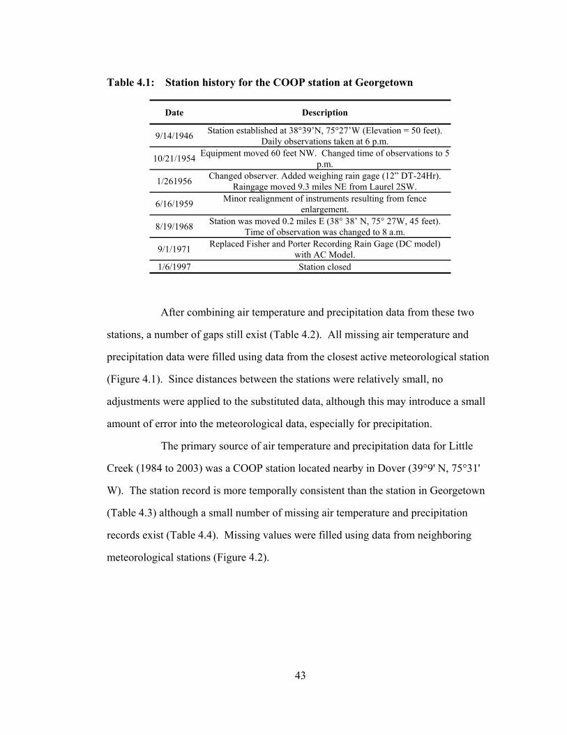
Table 4.1: Station history for the COOP station at Georgetown

Date Description

9/14/1946 Station established at 38°39’N, 75°27’W (Elevation = 50 feet). Daily observations taken at 6 p.m.

10/21/1954 Equipment moved 60 feet NW. Changed time of observations to 5 p.m.

1/261956 Changed observer. Added weighing rain gage (12” DT-24Hr). Raingage moved 9.3 miles NE from Laurel 2SW.

6/16/1959 Minor realignment of instruments resulting from fence enlargement.

8/19/1968 Station was moved 0.2 miles E (38° 38’ N, 75° 27W, 45 feet). Time of observation was changed to 8 a.m.

9/1/1971 Replaced Fisher and Porter Recording Rain Gage (DC model) with AC Model.

1/6/1997 Station closed

After combining air temperature and precipitation data from these two

stations, a number of gaps still exist (Table 4.2). All missing air temperature and

precipitation data were filled using data from the closest active meteorological station

(Figure 4.1). Since distances between the stations were relatively small, no

adjustments were applied to the substituted data, although this may introduce a small

amount of error into the meteorological data, especially for precipitation.

The primary source of air temperature and precipitation data for Little

Creek (1984 to 2003) was a COOP station located nearby in Dover (39°9' N, 75°31'

W). The station record is more temporally consistent than the station in Georgetown

(Table 4.3) although a small number of missing air temperature and precipitation

records exist (Table 4.4). Missing values were filled using data from neighboring

meteorological stations (Figure 4.2).

43

Table 4.2: Number of days with missing maximum and minimum air temperature and precipitation data at Georgetown

Year Maximum Temp.

Minimum Temp. Precip. Station(s) Used to Replace Missing Data

[number of days] 2003 0 0 0 2002 1 1 0 Greenwood 2NE [1] 2001 0 0 0 2000 0 0 0 1999 4 1 0 Greenwood 2NE [4] 1998 61 61 61 Greenwood 2NE [61] 1997 51 51 55 Greenwood 2NE [54], Jones Crossroads [1] 1996 172 172 172 Georgetown 5SW [172] 1995 30 30 30 Georgetown 5SW [30] 1994 0 0 0 1993 0 0 0 1992 0 0 3 Greenwood 2NE [3] 1991 0 0 0 1990 0 0 0 1989 0 0 2 Greenwood 2NE [2] 1988 3 3 0 Greenwood 2NE [3] 1987 0 0 0 1986 0 0 4 Milford 2SE [4] 1985 0 0 2 Milford 2SE [2] 1984 0 0 3 Milford 2SE [2], Bridgeville 1NW [1]

44

Figure 4.1: Location of meteorological stations used to create weather data set for Georgetown (1984 to 2003). National Weather Service COOP Stations are indicated by black triangles, Delaware Solid Waste Authority (DWSA) stations are indicated by red triangles, and the location of the Georgetown field trial and the Research and Education Center station is indicated by a blue triangle.

45

Table 4.3: Station history for the COOP station at Dover

Date Description

7/1/1870 Station established at 39°10’N, 75°32’W (Elevation = 34 feet). Observation time = 6 p.m.

9/26/1935 Changed time of observations to 5 p.m. 4/5/1951 Equipment moved 200 feet SE (Elevation = 30 feet)

5/8/1968 Station was moved 1.0 mile SE (39°9' N, 75°31' W, Elevation = 30 feet).

Table 4.4: Number of days with missing maximum and minimum air temperature and precipitation data at Dover

Year Maximum Temp.

Minimum Temp. Precip. Station(s) Used to Replace Missing Data

[number of days] 2003 0 0 0 2002 0 0 0 2001 0 0 0 2000 0 1 0 Milford 2SE [2] 1999 0 0 0 1998 0 0 0 1997 0 0 0 1996 0 0 0 1995 0 1 0 Georgetown 5SW [1] 1994 0 1 0 Georgetown 5SW [1] 1993 0 0 0 1992 0 0 0 1991 0 0 0 1990 0 0 0 1989 2 0 0 Milford 2SE [2] 1988 0 0 0 1987 1 1 1 Milford 2SE [1] 1986 0 0 0 1985 0 0 0 1984 0 0 0

46

Figure 4.2: Location of meteorological stations used to create weather data set for Little Creek (1984 to 2003). National Weather Service COOP Stations are indicated by black triangles and the location of the Little Creek field trial is indicated by a blue triangle.

47

4.2 Solar Radiation Data

Only a few stations in Delaware measured solar radiation data between

1984 and 2003. Therefore, the solar radiation dataset for Georgetown was constructed

using a combination of observed (daily solar radiation was recorded at the REC in

Georgetown between 1996 and 2003) and modeled data. In Georgetown, all of the

solar radiation data for 1984 to 1996 and all of the missing data between 1996 and

2003 were calculated using a solar radiation model (Table 4.5). All of the solar

radiation data for Little Creek was also calculated using a solar radiation model.

Several different solar radiation models have been developed to calculate

the amount of solar radiation incident on the earth’s surface using readily available

meteorological data (e.g., air temperature, precipitation, and cloud cover). A number

of the most commonly used solar radiation models were evaluated to determine the

most appropriate model for estimating daily solar radiation in Delaware. Pohlert

(2004) evaluated the impact of using modeled solar radiation on the yield predictions

of a maize growth simulation model. He tested three commonly used solar radiation

models developed by Ångström (1924), Bristow and Campbell (1984), and Allen

(1997). All three of these models were evaluated, in addition to a model developed by

Mahmood and Hubbard (2002).

48

Table 4.5: Number of days with missing solar radiation data at Georgetown

Year

Number of Days

Missing Solar

Radiation

Observed Data Source Missing Data Source

2003 29 Georgetown REC MH solar radiation model 2002 4 Georgetown REC MH solar radiation model 2001 0 Georgetown REC 2000 52 Georgetown REC MH solar radiation model 1999 40 Georgetown REC MH solar radiation model 1998 60 Georgetown REC MH solar radiation model 1997 81 Georgetown REC MH solar radiation model 1996 202 Georgetown REC MH solar radiation model 1995 All None MH solar radiation model 1994 All None MH solar radiation model 1993 All None MH solar radiation model 1992 All None MH solar radiation model 1991 All None MH solar radiation model 1990 All None MH solar radiation model 1989 All None MH solar radiation model 1988 All None MH solar radiation model 1987 All None MH solar radiation model 1986 All None MH solar radiation model 1985 All None MH solar radiation model 1984 All None MH solar radiation model

The Ångström model (1924) is a linear model that characterizes the

relationship between the ratio of the extraterrestrial solar radiation at the top of the

atmosphere (Ra) to solar radiation incident on the earth’s surface (Rg) and the ratio of

actual (n) to potential day length (N). Specifically,

Rg/Ra = a + b (n/N) (4.1)

49

where a and b are empirical regression coefficients. Ångström (1924) suggested

values of a = 0.2 and b = 0.5, however model calibration at different locations has

shown that these parameters vary significantly (Meza and Varas, 2000).

By contrast, the solar radiation model developed by Bristow and Campbell

(1984) is based on the relationship between diurnal temperature range and solar

radiation,

Rg/Ra = A (1 – exp [–B(dT)c]) (4.2)

where dT represents the diurnal temperature range – maximum daily air temperature

(°C) minus the minimum daily air temperature (°C) – and A, B, and C are empirical

regression coefficients. The Bristow and Campbell (Bristow and Campbell, 1984),

Allen model (Allen, 1997), and Mahmood and Hubbard (Mahmood and Hubbard,

2002) solar radiation models are all based on the relationship between diurnal

temperature range and solar radiation. Days with large diurnal temperature variations

are usually cloud-free and therefore will also received large amounts of solar

radiation. The coefficient A is the theoretical maximum radiation, while B and C

control the rate at which A is approached as the temperature difference increases. The

typical values of A, B, and C are 0.7, 0.004 to 0.010, and 2.4, respectively. However,

the values of these coefficients have been shown to vary geographically (Goodin et

al., 1999; Meza and Varas, 2000).

A modified version of the Bristow-Campbell model (hereafter modified B-

C) was developed by Goodin et al. (1999) and it is given by

Rg/Ra = A (1 – exp [–B(dTc/Ra)]) (4.3)

50

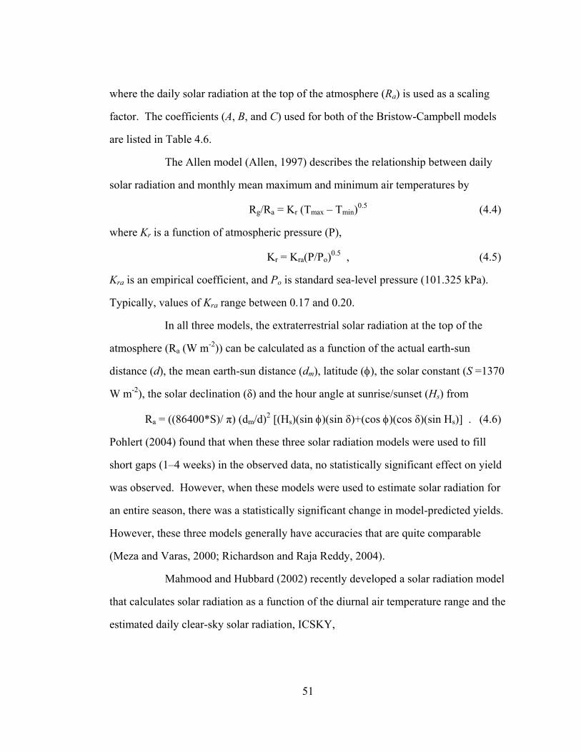
where the daily solar radiation at the top of the atmosphere (Ra) is used as a scaling

factor. The coefficients (A, B, and C) used for both of the Bristow-Campbell models

are listed in Table 4.6.

The Allen model (Allen, 1997) describes the relationship between daily

solar radiation and monthly mean maximum and minimum air temperatures by

Rg/Ra = Kr (Tmax – Tmin)0.5 (4.4)

where Kr is a function of atmospheric pressure (P),

Kr = Kra(P/Po)0.5 , (4.5)

Kra is an empirical coefficient, and Po is standard sea-level pressure (101.325 kPa).

Typically, values of Kra range between 0.17 and 0.20.

In all three models, the extraterrestrial solar radiation at the top of the

atmosphere (Ra (W m-2)) can be calculated as a function of the actual earth-sun

distance (d), the mean earth-sun distance (dm), latitude (φ), the solar constant (S =1370

W m-2), the solar declination (δ) and the hour angle at sunrise/sunset (Hs) from

Ra = ((86400*S)/ π) (dm/d)2 [(Hs)(sin φ)(sin δ)+(cos φ)(cos δ)(sin Hs)] . (4.6)

Pohlert (2004) found that when these three solar radiation models were used to fill

short gaps (1–4 weeks) in the observed data, no statistically significant effect on yield

was observed. However, when these models were used to estimate solar radiation for

an entire season, there was a statistically significant change in model-predicted yields.

However, these three models generally have accuracies that are quite comparable

(Meza and Varas, 2000; Richardson and Raja Reddy, 2004).

Mahmood and Hubbard (2002) recently developed a solar radiation model

that calculates solar radiation as a function of the diurnal air temperature range and the

estimated daily clear-sky solar radiation, ICSKY,

51

ICSKY = Is t (4.7)

which is the product of the clear-sky solar radiation, Is, and an empirical transmissivity

correction function, t. Clear-sky solar radiation, Is, can be calculated as a function of

latitude and Julian day (day of the year) from

Is = 0.04188 (A + B sin[2π (d + 10.5)/365 – (π/2)]) (4.8)

where Is is the clear-sky solar radiation (MJ m-2 day-1), d is the Julian day, and A and B

are location-dependent constants that can be estimated from

A = (sinφ (46.355 LD – 574.3885) + 816.41 cosφ sin[(π LD)/24]) (0.29 cosφ + 0.52) (4.9)

B = (sinφ (574.3885 – 1.509 LD) – 26.50 cosφ sin[(π LD)/24]) (0.29 cosφ + 0.52) (4.10)

where φ is the latitude and LD is the longest day of the year (in hours),

LD = 0.267 sin-1[0.5 + (0.007895/cosφ) + (0.2168875 tanφ)]0.5 . (4.11)

The empirical transmissivity correction function (t) is calculated from

t = 0.8 + 0.12 C1.5 (4.12)

where the transmissivity correction coefficient (C) is

C = |182 – d|/183 (4.13)

and again, d is the Julian day.

Table 4.6: Calibrated coefficients for the Bristow-Campbell and modified Bristow-Campbell solar radiation models (Goodin et al. 1999)

Coefficients Bristow-Campbell Modified B-C

A 0.68 0.75 B –0.03 –2.61 C 2.02 0.76

52

Mahmood and Hubbard (2002) evaluated their model two different

versions of the Bristow-Campbell model, the original version (Equation 4.2) and a

modified version proposed by Goodin et al. (1999) (Equation 4.3) at nine locations in

the Northern Great Plains (North Dakota, South Dakota, Nebraska, and Kansas).

Their model performed slightly better than the original Bristow-Campbell model and

much better than the modified B-C model (Table 4.7). The RMSE for the MH model

ranged from 3.53 to 4.78 MJ m-2 day-1 across the nine sites and the RMSE for the

Bristow-Campbell model ranged from 3.90 to 4.78 MJ m-2 day-1. This is comparable

to the results of Goodin et al. (1999) when they evaluated the Bristow-Campbell

model using 30 years of data for Manhattan, KS. In the Goodin et al. (1999) study,

the RMSE ranged from 2.0 to 6.2 MJ m-2 day-1 (26 to 47% error) across their ten sites.

Table 4.7: Comparison of model performance for three solar radiation models: Range of performance statistics across nine evaluation sites in the Northern Great Plains (Mahmood and Hubbard, 2002)

Model Performance Statistic MH Bristow-Campbell Modified B-C

RMSE (MJ m-2 day-1) 3.53 to 4.78 3.90 to 4.78 7.06 to 9.16 D index 0.94 to 0.91 0.94 to 0.90 0.67 to 0.56

Relative Error (%) 20 to 36% 22 to 37% 45 to 62%

Since the MH and Bristow-Campbell models have been shown to simulate

solar radiation adequately at other mid-latitude locations in the United States, both

models were evaluated against observed solar radiation data for Georgetown in 2003.

Results indicate the MH model simulated daily solar radiation much more accurately

than the Bristow-Campbell model (Tables 4.8 and 4.9). The simulated mean for the

MH model was closer to the observed data than the Bristow-Campbell model. The

53

MH model also had a lower RMSE, a higher index of agreement (D index) (Willmott,

1982; Willmott, 1984), and a higher coefficient of efficiency (E) (Legates and

McCabe, 1999). The Bristow-Campbell model overestimated both the magnitude of

daily solar radiation in Delaware and the variability (Figure 4.3). This suggests that

the MH model is the better model for simulating solar radiation in Delaware.

Further examination revealed that the original formulation of the MH

model tended to systematically underestimate the actual solar radiation (Figure 4.4).

This bias was removed by calculating the linear regression between the observed solar

radiation data and the MH model. The equation generated by the regression fit was

used to remove the systematic bias from the MH model (MH-Bias Adjusted). The

MH-Bias Adjusted model has a lower RMSE and relative error, and a higher D index

and coefficient of efficiency than the original MH model. Generally, the MH-Bias

Adjusted model provides a reasonable simulation of daily solar radiation for

Georgetown (Figure 4.5). The remaining error in the MH-Bias Adjusted model (as

measured by RMSE and relative error) is similar to that in other published model

evaluations (e.g., Mahmood and Hubbard (2002), Goodin et al. (1999)). Mahmood

and Hubbard (2002) hypothesize that much of the remaining error can be attributed to

variables that their model does not consider such as atmospheric pollution, dust

storms, elevation, and seasonal burning.

54

Table 4.8: Descriptive statistics of observed and modeled daily solar radiation (MJ m-2 day-1) at Georgetown

Descriptive Statistic

Observed Solar Radiation MH MH-Bias Adjusted Bristow-Campbell

Mean 12.11 11.07 12.11 16.58 Median 10.80 10.85 11.85 16.90

Variance 45.72 23.18 27.76 52.21

Table 4.9: Comparison of model performance for three solar radiation models at Georgetown in 2003. The D index is a measure of agreement between the observed and modeled data. A D index of 1.0 indicates perfect agreement with lower D index values indicating less agreement. Relative error [(RMSE/mean)*100] is expressed as a percentage. The coefficient of efficiency is another measure of model agreement where a value of 1.0 indicates perfect agreement.

Model Performance Statistic MH MH-Bias Adjusted Bristow-Campbell

RMSE (MJ m-2 day-1) 4.54 4.25 6.87 MAE (MJ m-2 day-1) 3.60 3.36 4.89

D index 0.84 0.87 0.78 Relative Error 42.5% 35.0% 41.4% Coefficient of Efficiency (E) 0.58 0.61 –0.03

55

Figure 4.3: Scatter plot of measured and modeled (Bristow-Campbell) solar radiation (MJ m-2 day-1) at Georgetown, DE in 2003. The red line corresponds to the perfect prediction line.

56

Figure 4.4: Measured (yellow line) and modeled (MH model = dark blue line; MH bias adjusted model = light blue line) daily solar radiation (MJ m-2 day-1) at Georgetown, DE in 2003.

57

Figure 4.5: Scatter plot of measured and modeled (Mahmood-Hubbard bias adjusted) daily solar radiation (MJ m-2 day-1) at Georgetown, DE in 2003. The red line corresponds to the perfect prediction line.

4.3 Calibrated Radar Precipitation Estimates

Agricultural modeling, like most hydroclimatological applications,

requires accurate estimates of precipitation at a high spatial resolution and often in

real-time. Traditionally, raingages have been used to provide in situ measurements of

precipitation at a single point. Although raingages can provide accurate point

estimates of precipitation, most precipitation networks are not dense enough to

provide the high spatial resolution required to resolve convective storms. Indeed,

most hydroclimatological applications and modeling activities require precipitation

58

data at a much higher spatial resolution than the existing gage network can supply.

Other sources of precipitation data exist. Since the 1970s, satellites have been

increasingly used to provide precipitation estimates as well as the development of the

National Weather Service’s (NWS) network of WSR-88D (Weather Surveillance and

Radar – 1988 Doppler) weather radars (Legates, 2000).

To capture the spatial variability in precipitation across Delaware,

raingage-calibrated radar precipitation estimates are used. These raingage-calibrated

estimates were chosen as the best source of precipitation data for this study since they

are available in real-time at a resolution of 4 km by 4 km (i.e., the Hydrological

Resources Analysis Project (HRAP) grid). The Delaware Environmental Observing

System (DEOS) resamples these estimates to a 1 arc-minute resolution (~2 km2)

during the calibration process (developed by Legates, 2000).

The WSR-88D is an active S-band microwave system that sends out a

beam of energy at a wavelength of approximately 10 cm and measures the backscatter

(reflected energy). Each WSR-88D radar makes a 360° azimuthal sweep at a variety

of elevation angles (ranging from 0.5–20°). During precipitation events the lowest

four angles (0.5°, 1.5°, 2.5°, and 3.5°) are merged into a single volume scan to

produce a composite of radar reflectivity (Z). In ‘precipitation modes’, the radar

produces a volume scan every six minutes (and every 15 minutes during ‘clear air

modes’). In addition to the standard precipitation mode, the radar also has two clear

air modes (where the radar scans at five different angles from 0.5–4.5°) and a severe

weather mode (where the radar scans at 14 different angles from 0.5–19.5°) (Fulton et

al., 1998).

59

The WSR-88D measures three basic quantities –– reflectivity, spectral

width, and mean radial velocity. From these three quantities, the NWS is able to

generate a suite of 39 meteorological products (Fulton et al., 1998; Klazura and Imy,

1993), although only reflectivity is used in precipitation estimation. Klazura and Imy

(1993) provide a complete discussion of the WSR-88D system and network while

Fulton et al. (1998) provide a detailed description of the rainfall estimation

algorithms.

The relationship between rainfall rate and reflectivity (Z; mm m ) is not

exact because rainfall rate is proportional to the volume of the raindrops while

reflectivity is proportional to the surface area of the drops. Therefore, the drop size

distribution is extremely important factor in determining the relationship between

rainfall rate and reflectivity. Generally, this drop size distribution is assumed and an

equation of the form

6 -3

Z = a Rb (4.14)

is used to estimate rainfall rates. In the above equation, a and b are coefficients, with

a generally ranging from 30 to 500 and b ranging from 1.2 to 2.0 (Legates, 2000).

Two main forms of the equation are commonly used for convective precipitation;

Z = 300 R1.4 (4.15)

is appropriate for estimating non-tropical convective rainfall, while

Z = 250 R1.2 (4.16)

is used for estimating rainfall from tropical convective systems. During non-

convective (stratiform) events three additional equations have been developed. For

warm-season stratiform events,

Z = 200 R1.6 (4.17)

60

is the equation used, while

Z = 130 R2.0 (4.18)

is used for cool season stratiform precipitation east of the continental divide and

Z = 75 R2.0 (4.19)

is used for cool season stratiform precipitation west of the continental divide. Raw

reflectivity values are processed by the WSR-88D system to produce the Digital

Precipitation Array (DPA). The DPA is a cartesian grid of approximately 4 km by 4

km that contain the reflectivity values for a one hour period. It is necessary to

calibrate the radar data supplied by the network of WSR-88D weather radars because

uncalibrated radar estimates have historically resulted in considerable underestimation

of heavy precipitation and overestimation of light precipitation (Legates, 2000).

4.4 Soils Data

The only soil dataset for Delaware that is available in a digital form is the

State Soil Geographic (STATSGO) database created by the Natural Resource

Conservation Service (NRCS). The STATSGO database was designed for broad

planning and management uses that cover state, regional, and multi-state areas. It was

produced by generalizing the detailed soil survey data to a mapping scale of 1:250,000

using the United States Geological Survey (USGS) 1:250,000 topographic

quadrangles as the base map. The number of soil polygons per quadrangle map ranges

from 100 to 400 and the minimum area mapped is roughly 625 hectares (1,544 acres).

The NRCS produces a higher resolution soil data (e.g., NRCS Soil Survey Geographic

Database (SSURGO)) that would be more appropriate for this study, but the Delaware

data has still not been released in a digital form.

61

Each of the soil polygons (or STATSGO map units (MUID)) depicts the

dominant soil type in the area and may consist of up to 21 component soils. Each of

the component soils has up to six layers and for each soil layer, data on 28 physical

and chemical properties are provided. This information is stored in a series of linked

tables (relational database). There are a total of 14 STATSGO map units within

Delaware (Table 4.10 and Figure 4.6).

Table 4.10: Description of STATSGO soil polygons (MUID) in Delaware. The dominant soil type is the most extensive soil component in each MUID. The percentage corresponds to the number of grid cells that fall within each MUID compared to the total number of grid cells in Delaware that are on agricultural land (e.g., 224).

STATSGO Map Unit (MUID) Dominant Soil Type Number of Grid Cells

Percentage of Agricultural Area in

Delaware DE001 Evesboro Loamy Sand 72 32.14% DE002 Pocomoke Sandy Loam 3 1.34% DE003 Sassafras Sandy Loam 29 12.95% DE004 Keyport Silt Loam 8 3.57% DE005 Matapeake Silt Loam 18 8.04% DE006 Woodstown Sandy Loam 1 0.45% DE007 Sassafras Sandy Loam 8 3.57% DE008 Fallsington Sandy Loam 2 0.89% DE009 Pocomoke Sandy Loam 19 8.48% DE010 Woodstown Sandy Loam 2 0.89% DE011 Fallsington Sandy Loam 42 18.75% DE012 Evesboro Loamy Sand 5 2.23% DE013 Matapeake Silt Loam 9 4.02% DE014 Pocomoke Sandy Loam 1 0.45% DE016 Matapeake Silt Loam 1 0.45% DE017 Chester Silt Loam 4 1.79%

A total of 310 HRAP grid cells lie within Delaware. The 2002 Land-

use/Land-cover (LULC) data were used to extract only those HRAP cells that were

62

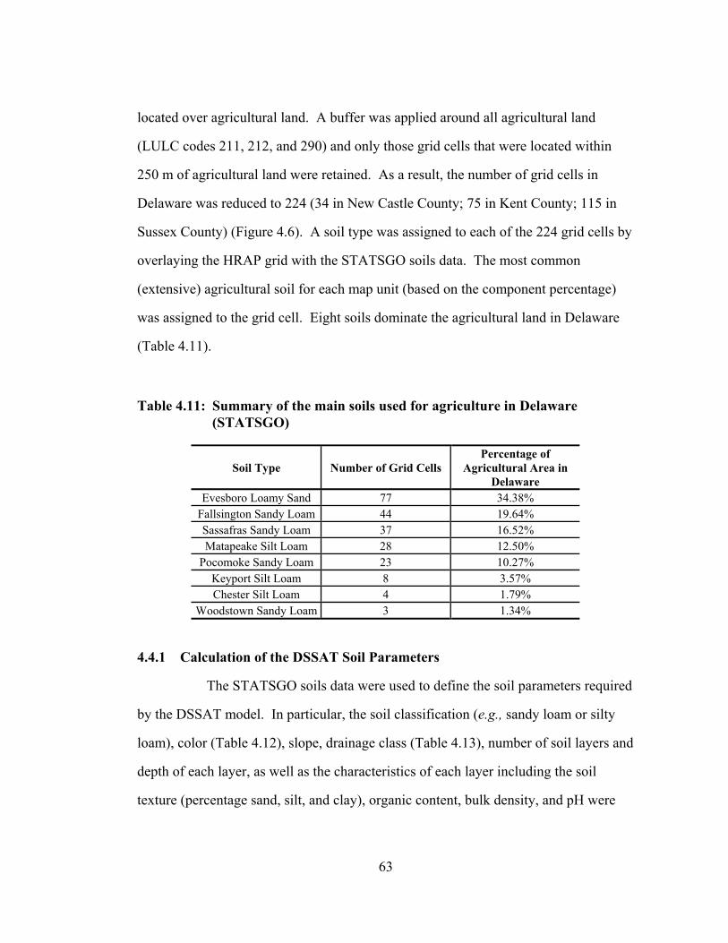
located over agricultural land. A buffer was applied around all agricultural land

(LULC codes 211, 212, and 290) and only those grid cells that were located within

250 m of agricultural land were retained. As a result, the number of grid cells in

Delaware was reduced to 224 (34 in New Castle County; 75 in Kent County; 115 in

Sussex County) (Figure 4.6). A soil type was assigned to each of the 224 grid cells by

overlaying the HRAP grid with the STATSGO soils data. The most common

(extensive) agricultural soil for each map unit (based on the component percentage)

was assigned to the grid cell. Eight soils dominate the agricultural land in Delaware

(Table 4.11).

Table 4.11: Summary of the main soils used for agriculture in Delaware (STATSGO)

Soil Type Number of Grid Cells Percentage of

Agricultural Area in Delaware

Evesboro Loamy Sand 77 34.38% Fallsington Sandy Loam 44 19.64% Sassafras Sandy Loam 37 16.52% Matapeake Silt Loam 28 12.50%

Pocomoke Sandy Loam 23 10.27% Keyport Silt Loam 8 3.57% Chester Silt Loam 4 1.79%

Woodstown Sandy Loam 3 1.34%

4.4.1 Calculation of the DSSAT Soil Parameters

The STATSGO soils data were used to define the soil parameters required

by the DSSAT model. In particular, the soil classification (e.g., sandy loam or silty

loam), color (Table 4.12), slope, drainage class (Table 4.13), number of soil layers and

depth of each layer, as well as the characteristics of each layer including the soil

texture (percentage sand, silt, and clay), organic content, bulk density, and pH were

63

extracted from the NRCS STATSGO database for each of Delaware’s eight main

agricultural soils. Once the slope, drainage class, and runoff potential were

determined from the

64

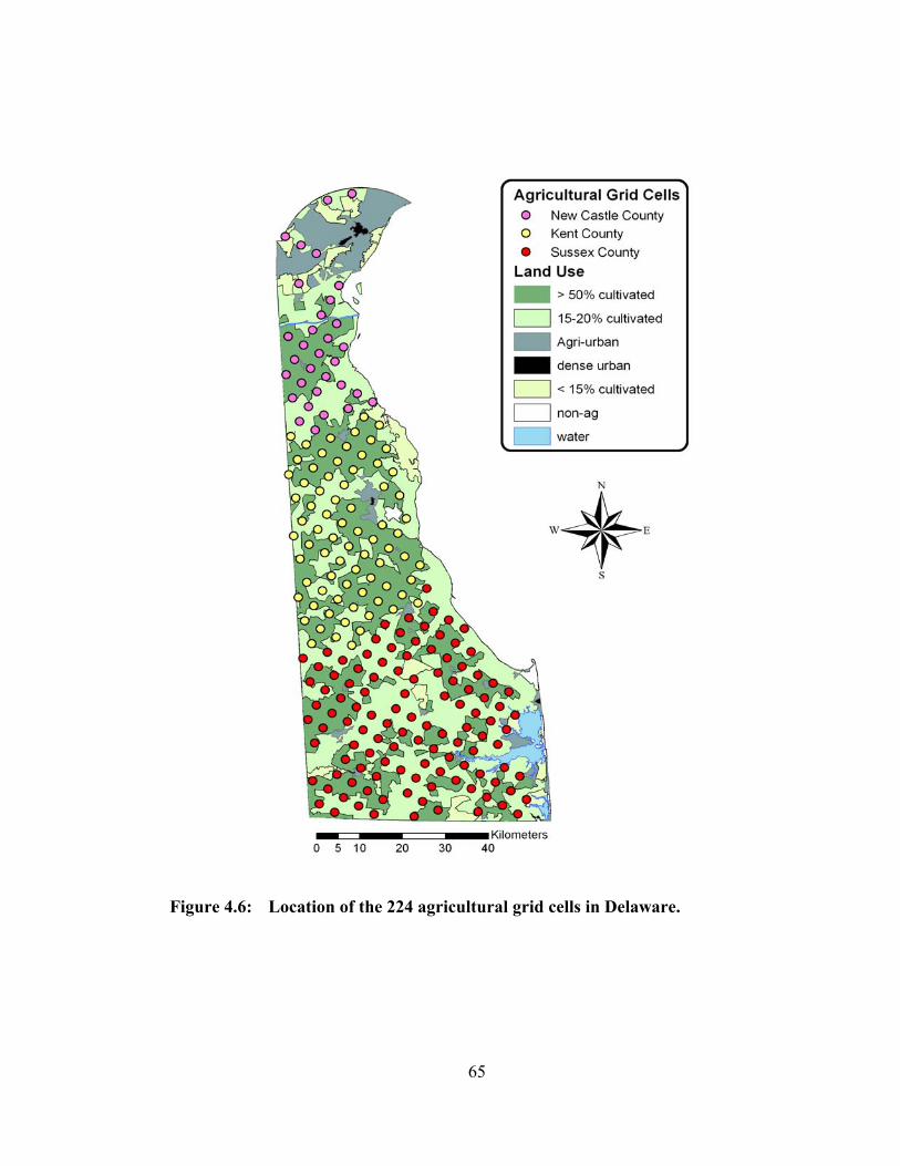
Figure 4.6: Location of the 224 agricultural grid cells in Delaware.

65

STATSGO database, DSSAT used these parameters to automatically calculate the

runoff curve number (Table 4.14).

It is recommended that the total number of soil layers in the DSSAT

model should be between 7 and 10 and that each layer of the soil should not exceed 30

cm in the lower part of the soil profile and 15 cm in the upper part of the soil profile

(Ritchie, 1998). The NRCS soil survey data only allow for a maximum of six layers

and each layer is usually much thicker than the DSSAT specifications (Table 4.15).

To conform to the DSSAT specifications, each of the actual soil layers was divided

into at least two additional layers having the same characteristics.

Table 4.12: Soil color and the associated DSSAT soil albedo

Soil Color Soil Albedo

Brown 0.13 Red 0.14

Black 0.09 Gray 0.13

Yellow 0.17

Table 4.13: NRCS drainage classes and the associated DSSAT drainage coefficient

Drainage Drainage Coefficient

Excessive 0.85 Somewhat Excessive 0.75

Well 0.60 Moderately Well 0.40 Somewhat Poor 0.25

Poorly 0.05 Very Poorly 0.01

66

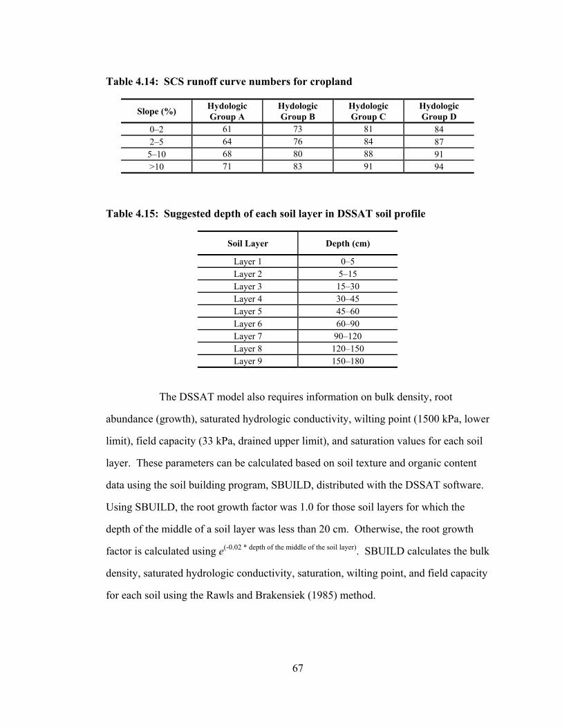
Table 4.14: SCS runoff curve numbers for cropland

Slope (%) Hydologic Group A

Hydologic Group B

Hydologic Group C

Hydologic Group D

0–2 61 73 81 84 2–5 64 76 84 87

5–10 68 80 88 91 >10 71 83 91 94

Table 4.15: Suggested depth of each soil layer in DSSAT soil profile

Soil Layer Depth (cm)

Layer 1 0–5 Layer 2 5–15 Layer 3 15–30 Layer 4 30–45 Layer 5 45–60 Layer 6 60–90 Layer 7 90–120 Layer 8 120–150 Layer 9 150–180

The DSSAT model also requires information on bulk density, root

abundance (growth), saturated hydrologic conductivity, wilting point (1500 kPa, lower

limit), field capacity (33 kPa, drained upper limit), and saturation values for each soil

layer. These parameters can be calculated based on soil texture and organic content

data using the soil building program, SBUILD, distributed with the DSSAT software.

Using SBUILD, the root growth factor was 1.0 for those soil layers for which the

depth of the middle of a soil layer was less than 20 cm. Otherwise, the root growth

factor is calculated using e(-0.02 * depth of the middle of the soil layer). SBUILD calculates the bulk

density, saturated hydrologic conductivity, saturation, wilting point, and field capacity

for each soil using the Rawls and Brakensiek (1985) method.

67

Gijsman et al. (2002) evaluated eight different methods for calculating

soil water parameters, including the Rawls and Brakensiek (1985) method, and

concluded that accurate soil water parameters can only be generated if the texture (and

organic matter) of each layer of the soil is precisely known. Using only soil type to

calculate soil water parameters may, depending on the textural class, result in large

errors in the input data. Their results also showed that estimates of the soil water

parameters vary greatly depending on the method used and the soil texture. For

example, the average error associated with estimating available water capacity using

only soil type was 0.05 cm3 cm-3. Unfortunately, small variations (e.g., 0.03 cm3 cm-3)

in available water holding capacity can be the difference between a good yield and a

poor yield. All eight of the methods that Gijsman et al. (2002) evaluated, had

difficulty accurately estimating soil water parameters for very coarse textured soils

(greater than 70% sand). This is of particular importance for this study since

Delaware soils are very sandy.

Gijsman et al. (2002) demonstrated that DSSAT yield predictions are

sensitive to the soil water parameters and in their experiments yield variations, even

within a single soil type (e.g., sandy loam), were as great as 3000 kg ha-1. Therefore,

the lack of high-resolution digital soils data for Delaware and the uncertainties

associated with estimating soil water parameters, particularly for sandy soils, are both

cause for concern. Clearly, the DSSAT crop yield models require accurate soil texture

data.

68

Chapter 5

SENSITIVITY OF THE CERES-MAIZE MODEL

Quantifying the sensitivity of the CERES-Maize model to uncertainties in

the input data is particularly important since yield will be simulated for all of

Delaware even though information on agronomic practices (e.g., row spacing, planting

density, planting date) are only readily available at the field-trial sites. Other input

data, such as air temperature and solar radiation, may also contain errors because the

air temperature data is based on a small number of point-specific in situ measurements

and the solar radiation data is based on model estimates. The impact that these

uncertainties have on the CERES-Maize model will be quantified for eight of the input

variables. Variables considered include row spacing, planting density, planting date,

initial soil moisture, carbon dioxide concentration, air temperature, solar radiation, and

soil type. Model sensitivity will be assessed for each these variables by measuring

how changing these variables affects yield. It should be noted that modifying the

input variables will not only affect yield, but also many other model-predicted

variables such as those related to crop growth (e.g., number of leaves, date of

maturity, plant height), nutrient uptake, and the water balance (e.g., available soil

moisture, evapotranspiration, and potential evapotranspiration). This model

sensitivity will focus explicitly on the impacts on crop yield because it is the only

variable for which we have detailed observational data. The sensitivity analysis is

69

based on 20 years of yield data (1984 to 2003) collected at the Georgetown field trial

site.

5.1 Row Spacing

Actual row spacing at the field-trial site in Georgetown is 75 cm. Model

sensitivity to variations in row spacing was tested using seven different possibilities

that ranged from 40 cm to 100 cm. Results show that as row spacing decreased, the

model-predicted yield increased, as expected (Table 5.1). When row spacing was 100

cm, yields decreased by an average of 2.7%, whereas yields increased by an average

of 3.9% when the row spacing was only 40 cm as compared to model-predicted yields

using the actual row spacing (75 cm). The results were consistent across all 20 years,

which indicates that the relationship between row spacing and yield is not affected by

weather conditions. Relatively large changes in row spacing have a relatively small

impact on yield (e.g., changing row spacing from 60 to 90 cm only changes mean

yields by 3%).

Table 5.1: Impact of row spacing on yield at Georgetown. The mean change in yield is calculated by comparing the mean yield (n = 20) using the actual row spacing (75 cm) to the mean yield resulting from each of the seven prescribed row-spacings.

Row Spacing 40 cm 50 cm 60 cm 70 cm 80 cm 90 cm 100 cm

Mean Change in Yield (kg

ha-1)

291.1 197.4 117.3 40.3 –38.8 –116.9 –200.9

Mean Change in Yield (%)

3.85 2.61 1.55 0.53 –0.51 –1.55 –2.66

70

5.2 Planting Density

Actual planting density at the field-trial site in Georgetown is 6.92 plants

m-2 (28,000 plants per acre). The sensitivity of the CERES-Maize model to variations

in planting density was tested using seven different densities that ranged from 2.47

plants m-2 to 9.88 plants m-2 (10,000 to 40,000 plants per acre). As planting density

decreased, the model-predicted yield also decreased (Table 5.2), as expected. A

planting density of 2.47 plants m-2 decreased yields by an average of 32.4% as

compared to model-predicted yields using actual planting density, while a planting

density of 9.88 plants m-2 increased yields by an average of 2.8%. However, the

results from individual years were significantly different than the mean because of the

interaction between weather conditions (especially those that affected the availability

of soil moisture) and planting density.

The model showed two main types of responses to changes in planting

density (Figure 5.1). In years that received ample precipitation, the model-predicted

yield increased as the planting density increased (e.g., 1984), while for years that

received limited precipitation, yield increased as planting density increased until it

eventually peaked and began to decline as planting density continued to increase.

Thus, the relationship between planting density and yield is strongly controlled by the

availability of soil moisture. During wet years, enough soil moisture exists to support

more plants and therefore increasing the planting density increases the observed yield

(the soil has a greater carrying capacity). Soil moisture availability is limited during

dry years. Therefore, increasing planting density beyond the carrying capacity results

in a decreased yield due to the competition for soil moisture. However, model

sensitivity results show that variations in planting density across Delaware (planting

71

density normally varies between 6.18 and 8.65 plants m-2) will have a relatively small

impact on yield (change mean yields by ~2%).

Table 5.2: Impact of planting density on yield at Georgetown. The mean change in yield is calculated by comparing the mean yield (n = 20) using the actual planting density (6.92 plants m-2) to the mean yield calculated using each of the seven prescribed planting densities.

Planting Density

2.47 plants m-2

3.71 plants m-2

4.94 plants m-2

6.18 plants m-2

7.41 plants m-2

8.65 plants m-2

9.88 plants m-2

Mean Change in Yield (kg

ha-1)

–2448.8 –825.4 –225.1 –61.8 18.1 75.4 209.2


–32.37 –10.91 –2.98 –0.82 0.24 1.00 2.77

Figure 5.1: Seeding density (plants m-2) versus yield (kg ha-1) for Georgetown

72

5.3 Planting Date

Planting at the field-trial site in Georgetown normally occurs on April 23

(1984 to 2003). The impact of planting date on yield was simulated using nine

different planting dates ranging from April 1 to May 27. In general, earlier planting

dates resulted in lower yields and later planting dates resulted in higher yields (Table

5.3). When the crop was planted on April 1 (roughly three weeks earlier than normal),

mean yield decreased by just over 1%. By contrast, when the crop was planted on

May 27 (roughly four weeks later than normal), mean yield increased by about 10%.

However, the results from individual years varied significantly due to the interaction

between weather conditions (especially those that affected the availability of soil

moisture) and planting date (Figure 5.2).

Changing the planting date modified the timing of phenological

development. In 1992, for example, the actual planting date was April 16. Using this

planting date, the model simulated that silking occurred on July 7 and grain fill

occurred between July 16 and August 25. The simulated yield was 7079 kg ha-1. But

when a planting date of May 26, 1992 (more than a month after the actual planting

date) was used, the model simulated that silking occurred on July 25 and grain fill

occurred between August 6 and September 17. The simulated yield for this planting

date was 12,779 kg ha-1, an increase of 5700 kg ha-1 over the earlier planting date.

The large in model-predicted yields is a result of the unequal distribution of

precipitation during the 1992 growing-season. Since corn is most susceptible to

moisture stress during the reproductive phases (flowering and silking), the timing of

these two growth phases in relation to the occurrence of precipitation is an important

factor that affects yield. In 1992, planting the crop a month later reduced the water

stress on the plant during the critical growth phases. Since the distribution of

73

precipitation within each growing season is different, it is difficult to generalize how

planting date will affect yield. In Delaware, however, the growing season is long

enough that the occurrence of frost is normally not a factor limiting crop growth and

ample heat and solar radiation are normally available. Therefore, the main cause of

variations in crop yield due to planting date occurs because of the interaction between

soil moisture availability (which is primarily driven by precipitation) and the growth

stage of the crop.

5.4 Initial Soil Moisture

Since no soil moisture information is available for any of the field trial

sites in Delaware, initial soil moisture conditions must be estimated. The sensitivity

of CERES-Maize to variations in initial soil moisture condition was tested by varying

the initial soil moisture conditions on January 1st from 10–100% of field capacity (not

shown). Initial soil moisture conditions had no impact on yield. Since the model

simulations for each year are started on January 1st, the impact of the initial soil

moisture conditions has abated by the time planting occurs in April. This is important

since DSSAT treats each year as a distinct event with no carryover to the next year.

Climatologically, however, this approximation is reasonable since winter precipitation

in Delaware is usually sufficient to bring the soil to field capacity by April 1.

74

Table 5.3: Impact of planting date on yield at Georgetown. The mean change in yield is calculated by comparing the mean yield (n = 20) using the actual planting date (6.92 plants m-2) to the mean yield using each of the nine prescribed planting dates.

Planting Date 1-Apr 8-Apr 15-Apr 22-Apr 29-Apr 6-May 13-May 20-May 27-May

Mean Change in Yield (kg ha-1)

–102.0 34.8 51.5 –18.3 264.7 426.7 473.5 740.7 941.0

Mean Change in Yield

(%)

–1.35 0.46 0.68 –0.24 3.50 5.64 6.26 9.79 12.44

Figure 5.2: Planting date (month/day) versus yield (kg ha-1) at Georgetown

75

5.5 Air Temperature

The sensitivity of CERES-Maize to variations in air temperature was

tested by varying observed air temperatures (both maximum and minimum air

temperatures) from +5°C to –5°C by 1°C. The temperature changes were applied so

that a +1°C temperature would result in all of the maximum and minimum daily

temperatures being increased by 1°C. The sensitivity of the DSSAT model to air

temperature is particularly important since site-specific meteorological observations

are not usually available. In general, the model-predicted yield is inversely related to

air temperature (Table 5.4), except for air temperature decreases of 4°C and 5°C. For

example, an air temperature decrease of 3°C increases yields by an average of 33.6%

(compared to model-predicted yields using actual air temperatures), while an air

temperature increase of 5°C decreases yields by an average of approximately 25.8%.

Although a significant amount of inter-annual variability in the response

to air temperature modifications exists, model results generally exhibit a curvilinear

response to air temperature changes (Figure 5.3). Modeled yields generally reach a

maximum at air temperatures that are a few degrees lower than the observed air

temperatures and yields decline as air temperatures vary around this maximum. Thus,

air temperature has a direct impact on the growth of the crop and the moisture stress

experienced by the crop.

As air temperatures are increased, the amount of moisture stress

experienced by the crop also increases, thus resulting in lower yields. As air

temperatures decrease, the growth and development of the crop is hindered (and the

possibility of frost damage at the beginning of the growing season increases) thus

resulting in lower yields. The optimum air temperature minimizes the amount of

moisture stress experienced by the crop and maximizes the amount of energy available

76

for growth and development. The most sensitive years to changes in air temperature

(e.g., 1990, 1991, and 1992) are those that experienced the greatest water stress during

the sensitive growth stages of the crop. Decreasing the air temperatures causes the

crop to develop more slowly and can result in higher yields since the timing of the

moisture sensitive growth stages is shifted later into the growing season. Reducing air

temperature has the same impact on the timing of crop development as delaying

planting (Section 5.3). Therefore, years most affected by changes in planting date are

also those affected most by changes in growing season air temperature (e.g., 1990,

1991, and 1992). Shifting the timing of crop development minimizes the impact that

these periods of moisture stress have on crop yield. During most years, however,

modifying the air temperature had a much less significant impact on yield since

precipitation was more evenly distributed throughout the growing season.

Table 5.4: Impact of air temperature on yield at Georgetown. The mean change in yield is calculated by comparing the mean yield (n = 20) using the actual air temperatures to the mean yield using each of the ten prescribed air temperature perturbations.

Temp. Change

–5 –4 –3 –2 –1 +1 +2 +3 +4 +5

Mean Change in Yield (kg ha-

1)

99.1 2078.5 2544.1 1430.0 737.4 –336.2 –866.5 –1124.2 –1660.0 –1948.4


(%)

1.31 27.48 33.63 18.90 9.75 –4.44 –11.45 –14.86 –21.94 –25.76

77

Figure 5.3: Temperature change (°C) versus yield (kg ha-1) at Georgetown

5.6 Solar Radiation

As discussed previously, measured solar radiation is only available for a

limited number of years therefore most of the solar radiation data is based on model

estimates. The impact of solar radiation on yield was simulated by changing solar

radiation +0.5 to +5.0 MJ m-2 day-1. The solar radiation changes were applied so that

a +1.0 MJ m-2 day-1 change would result in all of the daily solar radiation values being

increased by +1.0 MJ m-2 day-1. As expected, as solar radiation was increased, the

model-predicted yield also increased (Table 5.5). Increasing daily solar radiation

inputs by 5.0 MJ m-2 day-1 increased yields by an average of 3.49% (compared to

78

model predicted yields using actual solar radiation). Increases in yield were relatively

consistent for most years, although some variability (e.g., for some years, yield

decreased as solar radiation increased) was caused by the impact of increases in solar

radiation on plant moisture stress. Increasing solar radiation increases the rate of

photosynthesis, which increases plant transpiration. During years when soil moisture

was sufficient, increases in solar radiation resulted in increased plant growth (and

resulted in higher yields). However, during years when soil moisture was limited,

increases in solar radiation resulted in increased water stress, thereby reducing yield.

In most years, relatively large changes in solar radiation had a relatively small impact

on yield (e.g., increasing solar radiation by 5.0 MJ m-2 day-1 increased mean yields by

3.49%). It is also important to note that solar radiation does not affect the timing of

phenological development since the model calculates phenological development based

solely on growing degree-days (air temperature).

Table 5.5: Impact of solar radiation (MJ m-2 day-1) on yield at Georgetown. The mean change in yield is calculated by comparing the mean yield (n = 20) using the actual solar radiation to the mean yield using each of the ten prescribed increases in solar radiation.

Solar Change (MJ m-2 day-1)

+0.5 +1.0 +1.5 +2.0 +2.5 +3.0 +3.5 +4.0 +4.5 +5.0


1)

72.3 107.6 113.3 129.5 205.9 226.5 247.8 264.3 238.4 263.8


(%)

0.96 1.42 1.50 1.71 2.72 2.99 3.28 3.49 3.15 3.49

79

5.7 Carbon Dioxide Concentration

The sensitivity of CERES-Maize to variations in carbon dioxide was

tested by increasing carbon dioxide concentrations 10 to 100 ppm (above the default

value of 330 ppm). As expected, model-predicted yields increased as carbon dioxide

concentrations increased (Table 5.6). Increasing the carbon dioxide concentration by

100 ppm (to 430 ppm) increased yields by an average of 8.4%. The observed

increases in yield were very consistent for all years because the growth response of the

CERES-Maize model to changes in the concentration of CO2 is explicitly defined

using species-specific coefficients. For maize, the growth response is linear for CO2

concentrations between 330 and 990 ppm. Using a constant carbon dioxide

concentration of 330 ppm for all years may cause a small systematic bias in yield

predictions. Between 1984 and 2003, mean annual concentrations of atmospheric

carbon dioxide increased from 344.4 ppm to 375.6 ppm according to observations

from in situ air samples collected at Mauna Loa Observatory, Hawaii. Thus, the 30

ppm increase in atmospheric carbon dioxide concentration during the last 20 years

would roughly produce a 2.5% increase in yields. For purposes of model validation

(Chapter 7), observed concentrations of atmospheric carbon dioxide will be used.

5.8 Soil Type

The sensitivity of CERES-Maize to variations in soil type was evaluated

using ten different soils. Nine of the soils are generic soils distributed with DSSAT

while the tenth soil type, representative of the soils found in southern Delaware, was

derived using the Natural Resources Conservation Service’s (NRCS) State Soil

Geographic (STATSGO) database. The nine DSSAT soils represent three common

80

Table 5.6: Impact of CO2 concentration (ppm) on yield at Georgetown. The mean change in yield is calculated by comparing the mean yield (n = 20) using a concentration of 330 ppm to the mean yield using each of the ten prescribed increases in CO2 concentration.

CO2 Change

(ppm) +10 +20 +30 +40 +50 +60 +70 +80 +90 +100


1)

59.5 115.1 173.0 246.7 314.4 379.3 434.3 505.5 569.2 635.5


(%)

0.79 1.52 2.29 3.26 4.16 5.01 5.74 6.68 7.52 8.40

texture classes, each at three different depths and the tenth soil, a Woodstown sandy

clay loam, is the actual soil found at the field trial site in Georgetown.

Soil depths for the ten soils used in the sensitivity analysis varied from 60

to 210 cm (Table 5.7). Soil texture varied from sandy loam (coarse textured) to silty

clay (fine textured). The depth, texture, and amount of organic material determine the

available water holding capacity (AWC) of the soil (or the amount of plant extractable

water). DSSAT defines the AWC of the soil as the difference between field capacity

and the permanent wilting point. The AWC is the maximum amount of plant available

water that the soil can hold against the influence of gravity. The AWC of the ten soils

evaluated varied from 6.0 to 28.4 cm. Generally, fine textured soils (soils dominated

by clay and silt) can hold more water than coarse textured soils (soils dominated by

sand); however, much of this soil water is not usable by plants because it is tightly

bound to soil particles. Therefore, while the upper and lower limits were much higher

for the fine textured soils, the AWC was not.

81

Saturation is the total amount of water that the soil could hold if all of the

available pore space in the soil was completely filled with water. Although the pore

spaces are smaller in fine textured soils, there are more of them, so they are able to

hold a greater amount of water. Saturation varied from 21.6 to 97.1 cm, with the

highest values found in the fine-textured clay soils. Coarse textured soils tend to drain

more quickly than fine textured soils because they have more macropores (while fine

textured soils have more micropores). The drainage rate varied from 0.1 to 0.6

(unitless coefficient, higher values indicate that infiltration occurs more quickly), with

the highest rates found in the coarse-textured sandy soils.

Table 5.7: Characteristics of the ten soils used in the model sensitivity analysis.

Soil Type Depth of the Soil

(cm)

Lower Limit (cm)

Upper Limit (cm)

Saturat. (cm)

Extract. Water (cm)

Albedo SCS

Curve Number

Drainage Rate

Woodstown Sandy Clay

Loam 175 11.7 28.0 48.8 16.3 0.13 76 0.4

Deep silty clay 210 52.9 80.6 97.1 27.7 0.11 85 0.3

Medium silty clay 150 37.4 58.6 69.2 21.2 0.11 87 0.2

Shallow silty clay 60 14.3 23.7 27.7 9.4 0.11 89 0.1

Deep silty loam 210 17.1 38.1 94.7 20.1 0.12 77 0.4

Medium silty loam 150 13.8 27.7 67.6 13.9 0.12 79 0.3

Shallow silty loam 60 6.2 12.2 27.1 6.0 0.12 81 0.2

Deep sandy loam 195 13.7 42.0 61.2 28.4 0.21 60 0.6

Medium sandy loam 150 16.0 32.6 54.0 16.6 0.13 70 0.5

Shallow sandy loam 60 3.8 11.0 21.6 7.3 0.13 74 0.4

82

Deep soils generally resulted in higher yields for all texture classes and

the deep sandy loam soil had the highest average yields of all ten soils evaluated

(Table 5.8). It was the only soil that performed better than the Woodstown sandy clay

loam (actual soil at Georgetown). The deep sandy loam had a larger AWC (284 mm

versus 163 mm) and a higher infiltration rate (lower SCS curve number and higher

drainage rate) than the Woodstown sandy clay loam. The shallow silty clay, shallow

silty loam, and shallow sandy loam soils produced the lowest yields (–39.8%, –38.4%,

and –33.2% less than the yields with the Woodstown sandy clay loam, respectively).

Thus, soil depth has a major influence on crop yield since deeper soils have higher

AWC and soils with higher AWC are more drought resistant. That is, the larger the

reservoir of soil moisture, the longer that a crop can withstand water stress. The

amount of water stress that a crop experiences is directly correlated with yield. Silty

clay and silty loam soils had average yields at each soil depth that were similar while

sandy loams had higher yields than both the silty clay and silt loam soils. Differences

were particularly pronounced for the medium and deep soils.

During 1989, 1996, 1997, 2000, and 2003, very little difference in final

yield was simulated among the ten different soil types. These years were all relatively

wet growing seasons where no crop moisture stress occurred during the moisture

sensitive growth stages. The consistent supply of moisture throughout the growing

season reduced the impact of the AWC on yield. For example, in 1989, the difference

between the largest yield and smallest yield was only 47 kg ha-1 (a difference of

0.5%). The largest differences in yield occurred during years with little precipitation

or when precipitation did not occur during the moisture sensitive stages of growth

83

(e.g., 1992, 1994, 1998, 1999). In 1994, the yield for the shallow silty clay soil was

4340 kg ha-1

Table 5.8: Impact of soil type on yield at Georgetown. The mean change in yield is calculated by comparing the mean yield (n = 20) using the actual soil (Woodstown Sandy Clay Loam) to the mean yield using each of the nine soil types.

Soil Type Mean Change in Yield (kg ha-1)


Deep silty clay –1245.9 –16.5 Medium silty clay –1675.7 –22.2 Shallow silty clay –3010.5 –39.8 Deep silty loam –1392.3 –18.4

Medium silty loam –1364.5 –18.0 Shallow silty loam –2907.5 –38.4 Deep sandy loam 1180.4 15.6

Medium sandy loam –553.0 –7.3 Shallow sandy loam –2513.8 –33.2

and the yield for the deep sandy loam soil was 12,320 kg ha-1. The difference between

the largest and smallest yield was 7980 kg ha-1 (a difference of 284%). When extreme

yield variability was related to soil type, total precipitation during the growing season

was less important than the temporal distribution of precipitation within the growing

season. If conditions were dry during silking and grain fill, yields were adversely

affected, especially in the shallow soils, since they respond rapidly to weather

conditions. Shallow soils reach field capacity after small amounts of precipitation and

can dry out in short time periods with insufficient precipitation.

84

5.9 Summary of Model Sensitivity

Model sensitivity was quantified for row spacing, planting density,

planting date, initial soil moisture, carbon dioxide concentration, air temperature, solar

radiation, and soil type. As row spacing increases and planting density decreases,

yields generally decrease, as expected. However, CERES-Maize is not overly

sensitive to row spacing or planting density, at least over the range of values normally

encountered in Delaware. Therefore, the seeding density and row spacing used at the

field-trial sites will be used for the model evaluation (Chapter 7). Planting date also

had a small impact on yield during most years. However, planting date can have a

large impact on yield when precipitation is unequally distributed throughout the

growing season because of the importance of the timing of dry spells in relation to the

growth stage of the crop.

The impact of air temperature on yield was similar to that of planting date

because both variables affect the timing of crop growth. Crop yield was particularly

sensitive to changes in temperature during years when precipitation was unevenly

distributed throughout the growing season. Although crop yield was quite sensitive to

large changes in temperature (e.g., +/–5°C), there should only be a small amount of

error in air temperature measurements (<1°C) since air temperature fields are

relatively homogenous during the summer and Delaware has minimal topographic

variability. Therefore, errors in the measurement of air temperature will only have a

minor impact on yield.

The sensitivity evaluation also established that initial soil moisture

conditions have no impact on yield. Therefore, for the purposes of crop yield

prediction (Chapter 8), starting the model on January 1 (more than 4 months prior to

planting) is appropriate for initializing soil moisture. However, since soil moisture

85

conditions are also monitored, it may be better to carry over the actual soil moisture

values from the previous year to more accurately represent soil moisture conditions

during the first few months of the year. Solar radiation also tends to have a relatively

small impact on yield, although the impact was greater during dry years. Higher

amounts of solar radiation generally resulted in higher yields. If the errors in the

modeled-predicted solar radiation values are randomly distributed, then solar radiation

should only have a minor impact on yield.

Also as expected, yield increased as carbon dioxide concentrations

increased. Since mean annual concentrations of atmospheric carbon dioxide increased

from 344.4 ppm to 375.6 ppm between 1984 and 2003 (as measured in Hawaii), a

small systematic bias may be introduced into the yield predictions. According to

CERES-Maize, a 30 ppm increase in carbon dioxide concentration results in a 2.5%

increase in yield. Therefore observed concentrations of atmospheric carbon dioxide

are used for the model validation (Chapter 7).

CERES-Maize is extremely sensitive to soil type. Shallow soils had

yields that were, on average, 40% lower than the yields calculated using the actual soil

at the field trial site. The amount of precipitation and the timing of precipitation in

relation to the crop growth determined how much soil type influenced yield. Soil type

did not affect yield when precipitation was abundant and evenly distributed over the

growing season. However, soil type had a major impact on yield during dry years

when precipitation was unevenly distributed over the growing season (especially if it

was lacking during the moisture sensitive growth stages). During one year, variations

in soil type caused yield differences of nearly 300%. Yield is more sensitive to soil

type than it is to row spacing, seeding density, date of planting, initial soil moisture,

86

air temperature, solar radiation, or carbon dioxide concentration. Unfortunately, soil

type is known with the least certainty since high-resolution digital soil data (e.g.,

SSURGO data) are currently unavailable for Delaware. The STATSGO data is also

too coarse to adequately capture the true distribution of soils in Delaware and it only

provides a range of values for each of the soil parameters. The inability to accurately

characterize soil type may introduce significant errors into the modeling process.

87

Chapter 6

SOIL MOISTURE VALIDATION

In addition to simulating crop yield, the Agricultural Drought Monitoring

System (ADMS) provides near-real-time estimates of soil moisture across Delaware.

With multi-component models such as CERES-Maize, each component must be

evaluated separately (Akinremi and McGinn, 1996c). In this chapter, the soil moisture

component of DSSAT (CERES-Maize) will be evaluated to determine how well the

model simulates observed soil moisture conditions.

6.1 The Importance of Soil Moisture

Soil moisture controls the exchange of mass and energy between the

atmosphere and the land surface (Basara and Crawford, 2002). When an ample supply

of soil moisture exists, water evaporates as the ground is heated (by solar radiation)

and plants use water for photosynthesis, which is released through the plant stomates

during respiration. Thus, the surface remains cooler (i.e., due to an increase in the

latent heat flux). If the soil is dry, all of the incoming solar radiation is used to warm

the soil making it hotter and drier (i.e., due to an increase in the sensible heat flux).

Therefore, the soil water content in the root zone is directly correlated with the

magnitude of the sensible and latent heat fluxes (Basara and Crawford, 2002). In

addition, the albedo and thermal diffusivity of a soil are also regulated by soil

moisture. A moist soil has a lower albedo than dry soil while the thermal diffusivity

88

of the soil (the rate of heat flow into the soil) will initially increase as the soil begins

to dry out, but then decreases when the soil becomes very dry.

Soil moisture directly leads to increased evaporation and transpiration

(Mo and Juang, 2003). Due to changes in albedo and moisture availability, soil

moisture anomalies, especially if they are strong and persistent, can play a role in both

creating and prolonging growing season droughts (Herring, 2000). Modeling studies

have demonstrated the importance of antecedent soil moisture conditions in initiating

and maintaining growing season droughts (Koster et al., 2003; Ogelsby and Erickson,

1989; Trenberth and Guillemot, 1996). However, the strength of the relationship

between precipitation and soil moisture varies by season and location (Mo and Juang,

2003).

Entin et al. (2000) identified two main scales of soil moisture variation.

Small-scale variations in soil moisture are primarily determined by soil type,

topography, vegetation, and root structure, while large-scale variations are mainly

dictated by atmospheric forcing. The atmosphere controls the supply of moisture to

the soil through precipitation and the demand from the soil through evapotranspiration

(which is determined by solar radiation, air temperature, wind speed, and relative

humidity).

Soil moisture is of agronomic importance because it regulates seedling

emergence, evapotranspiration, runoff, leaching, and crop yield (Akinremi and

McGinn, 1996c). Soil moisture also influences the occurrence of plant diseases. For

example, it is strongly correlated to outbreaks of the fungal infection Sclerotina in

canola (Wilson, 2002), and pest outbreaks (e.g., grasshoppers and mosquitoes). The

89

hydrologic cycle is also partly controlled by soil moisture since it influences the

amount of infiltration, runoff, and evapotranspiration (De Jong and Bootsma, 1996).

6.2 The DSSAT Soil Moisture Model

The DSSAT soil water model, originally developed by Ritchie and Otter

(1985) and subsequently modified (Jones, 1993; Jones and Ritchie, 1991; Ritchie,

1998), computes, on a daily basis, all of the processes that directly affect water content

in the soil profile. This one-dimensional model computes the daily changes in water

content ( ) in a soil profile with up to 20 soil layers using S∆

DRETIPS −−−−+=∆ (6.1)

where soil water is added to the soil profile by precipitation (P) and irrigation (I) and

is removed by plant transpiration (T), soil evaporation (E), root absorption (R), and

drainage (D) (also known as percolation). The soil water content of an individual soil

layer also increases/decreases through flow (either unsaturated flow or vertical

drainage) from/to an adjacent layer.

The model requires parameters that describe the surface conditions of the

soil and the characteristics of the soil layers. In particular, the DSSAT soil water

model requires information on the soil texture classification (e.g., silt loam, sandy

loam, loamy sand), color, slope, drainage class, the number of layers and the depth of

each layer. For each soil layer, the model requires the texture (percentage sand, silt,

and clay), organic content, bulk density, pH, relative root abundance/growth, saturated

hydrologic conductivity, lower limit of water availability (wilting point (1500 kPa)),

drained upper limit (field capacity (33 kPa)), and saturation.

Daily soil water infiltration is computed by subtracting surface runoff

from daily rainfall (and irrigation). The Soil Conservation Service (SCS) curve

90

method is used to partition rainfall into runoff and infiltration based on a curve

number that accounts for texture, slope, and tillage. A modified version of this

method, developed by Williams et al. (1984), is used in the DSSAT soil water model

to account for layered soils and soil water content at the time when rainfall occurs.

When a layer’s soil water content is greater than the drained upper limit, the model

uses a cascading approach for computing vertical soil water drainage. Drainage

through the profile is first computed based on an overall soil drainage parameter that

is constant with depth. The amount of water passing through each layer is then

constrained by the saturated hydrologic conductivity of that layer. Therefore, if the

computed drainage into a layer is greater than the saturated hydrologic conductivity,

water accumulates above that layer. This allows the model to simulate poorly drained

soils and perched water tables. Upward unsaturated flow is simulated in the model

using a conservative estimate of the soil water diffusivity and it is calculated based on

differences in the volumetric soil water content of adjacent layers (Ritchie, 1998).

Evaporation from the soil surface, root water uptake, and plant

transpiration are based on methods developed by Ritchie (1972). Four options for

calculating potential evapotranspiration (PE) are included in the DSSAT soil water

model. The Priestley-Taylor method (Priestley and Taylor, 1972) is a simplified form

of the Penman method (Penman, 1948) and the least data intensive of the four PE

methods, as it requires only daily values of net solar radiation and daytime air

temperature. The Priestley-Taylor method (1972) is

γ

ρ+∆∆

= nswvt

RPELc

26.1 (6.2)

where PEs is the surface-dependent potential evaporation (mm d-1), ct is a conversion

constant (0.01157 W m d MJ-1 mm-1), Lv is the latent heat of vaporization (2448.0 MJ

91

Mg-1), Rn is the net radiation (W m-2), γ is the psychrometer constant (0.067 kPa K-1),

ρw is the density of water (1 Mg m-3), and ∆ is the slope of the saturation vapor

pressure versus air temperature curve (kPa K-1). Daytime air temperature is

approximated from daily maximum and minimum air temperatures and daily net solar

radiation is computed by adjusting total solar radiation to account for the combined

albedo of the soil and plant canopy. The model determines soil albedo using the

specified soil color. Plant canopy albedo is a function of the leaf area index (LAI) of

the crop (a parameter calculated by the model). The slope of the saturation vapor

pressure versus air temperature curve, ∆, is calculated using

( )23.237

3.23727.17exp6108.04098

+

+⋅

⋅

TT

T

=∆ . (6.3)

More details on how the Priestley-Taylor method was implemented in the DSSAT soil

moisture model can be found in Ritchie (1972) and Jones and Ritchie (1991).

Two of the other methods for calculating PE are based on the traditional

Penman (1948) approach. The original Penman method (also referred to as FAO–24)

uses a combination of an energy-budget and an aerodynamic approach to estimate PE

γγρ

ρ+∆

++∆= aawtn

rwvtDUcR

PELc)54.0.1(6.2

(6.4)

where PEr is the reference-surface potential evaporation (mm d-1), Ua is the wind

speed at reference height (m s-1), Da is the vapor pressure deficit (kPa), and all other

variables are as defined above. By contrast, the Penman-Montieth equation

(Monteith, 1973) is a modified version of the Penman method that also accounts for

plant physiology, in addition to air temperature, wind speed, humidity, and solar

radiation influences, in estimating PE

92

)/(

/

ac

aapnswvt rr

rDcRPELc

γγρ

ρ++∆

+∆= (6.5)

where PEs is the surface-dependent potential evaporation (mm d-1), ρ is the density of

air (1.234 kg m-3), ra is the aerodynamic resistance (s m-1), rc is the canopy resistance

(s m-1), and all other variables are as defined above. It was adopted as the standard

method for measuring PE (or reference ET) by the Food and Agricultural Organization

of the United Nations (FAO) in 1990 (Allen et al., 1998). The FAO–56 application of

the Penman-Monteith equation is widely used because it is a physically based

approach that can be applied globally without additional parameter estimations. This

method has been extensively evaluated using lysimeter data and it has been

implemented in a wide range of applications (Droogers and Allen, 2002; Federer et

al., 1996). Although the Penman-Montieth equation may be the most accurate method

for estimating PE, it requires accurate meteorological data that is not readily available.

The fourth method for determining PE is the energy balance method

R SLEHn ++= (6.6)

where Rn is the net radiation, S is the soil heat flux, H is the sensible heat flux, and LE

is the latent heat flux. The amount of evaporation is estimated by measuring each

component of the energy balance and then calculating how much water could be

evaporated by the latent heat flux. This method requires flux data that is not readily

available. Given the data constraints, the Priestly-Taylor method for estimating PE

will be employed since it only requires daily air temperature and solar radiation data.

Once PE has been calculated, it is partitioned into potential soil

evaporation and potential plant transpiration based on the LAI (Jones et al., 2003).

After the soil surface is wetted from rainfall or irrigation, actual soil evaporation is the

minimum of the potential and soil-water-limiting calculations. If the soil surface is

93

dry, the difference between the actual and potential amount of soil evaporation is

added to the amount of potential plant transpiration to account for the increased heat

load on the canopy (Ritchie, 1972).

To determine whether the soil or atmosphere limits plant transpiration,

potential root water uptake is computed by calculating a maximum water flow to roots

in each layer and summing these values (Jones and Ritchie, 1991; Ritchie, 1998;

Ritchie and Otter, 1985). Potential root water uptake accounts for differences in root

density and soil water content in each layer and it also considers the impact of soil

texture on hydrologic conductivity. Actual plant transpiration, then, is the minimum

of potential plant transpiration and potential root water uptake. Therefore, the

atmosphere can limit transpiration when air temperatures or solar radiation are

inadequate, while the canopy can limit transpiration when the crop is not well

developed (low LAI), and the soil can limit transpiration when the soil is dry or root

density is low. Computing actual evapotranspiration (ET) using this method provides

a means of simulating water stress in the plant without explicitly modeling the water

content and water movement within the plant. If the ratio of ET/PE is less than 1.0,

the crop would have reduced stomatal conductance to prevent desiccation. The rate of

photosynthesis varies proportionately with the ratio of ET/PE, which simulates the

impact that plant water stress has on crop growth. The model also uses a ratio of

potential root water uptake and potential transpiration to regulate plant turgor and

expansive growth of crops. As soil water becomes more limiting, turgor pressure in

the leaves decreases and leaf expansion is affected.

94

6.3 Description of the Validation Study

In Delaware, little soil moisture data exists that is appropriate for model

validation. To validate the DSSAT soil moisture model, data were acquired from the

Natural Resources Conservation Service’s (NRCS) Soil and Climate Analysis

Network (SCAN) site located in Powder Mill, MD (39°1' N, 76°51' W) (Figure 6.1).

This site is useful because it is proximate to Delaware (i.e., a similar climate) and

shares similar soils. Hourly weather and soil moisture data for the SCAN site at

Powder Mill are available since 2002 at five depths – 2 inches (5 cm), 4 inches (10

cm), 8 inches (20 cm), 20 inches (50 cm), and 40 inches (100 cm).

Figure 6.1: Location of the NRCS SCAN site at Powder Mill, MD (indicated by red triangle).

95

Daily maximum and minimum air temperatures were derived from the

hourly data collected at the SCAN site in Powder Mill. Daily precipitation data were

taken from a COOP station located in Beltsville, MD (39°2' N, 75°56' W), and solar

radiation was calculated using the MH model.

Detailed soils data are also available for this site. The soil survey data

was used to define the input soil data required to run the DSSAT model. In particular,

the soil classification, color, slope, drainage class, number of layers and depth of each

layer, as well as the characteristics of each soil layer, such as the texture (percentage

sand, silt, and clay), organic content, bulk density, and pH were extracted from the

NRCS soil survey. The DSSAT model also requires information on root abundance

(growth), saturated hydrologic conductivity, wilting point (lower limit), field capacity

(drained upper limit), and saturation. Although this information is available from the

NRCS soil survey, for consistency, soil texture and organic content data were used to

calculate the saturated hydrologic conductivity, wilting point (lower limit), field

capacity (drained upper limit), saturation, and relative root abundance for each layer

of the soil using the methods described in Section 4.5. This was done to insure that

the methods used for the soil moisture validation are identical to the methods that will

be used to simulate soil moisture in real-time. Differences between the calculated and

laboratory-measured values of the soil parameters (e.g., field capacity, wilting point,

saturation, and available water holding capacity of the soil) will have a direct impact

on the performance of the DSSAT soil moisture model since they affect the amount of

water the soil can hold in each layer, the total available water holding capacity of the

soil, and the amount of water that is available to plants (Table 6.1). For example,

according to the NRCS soil survey, the sandy loam soil at the SCAN site has an

96

available water holding capacity of 120 mm while the calculated available water

holding capacity (based on the methods described in Section 4.5) is 100 mm. Part of

this difference is due to the difficulties involved in estimating AWC in course-textured

soils (e.g., sandy soils) (Gijsman et al., 2002). The NRCS also uses a different

threshold for field capacity and permanent wilting than DSSAT to determine AWC.

The NRCS thresholds for field capacity and permanent wilting point are 10 kPa and

1500 kPa, while the DSSAT thresholds are 33 kPa and 1500 kPa.

Table 6.1: Measured versus calculated (estimated) field capacity, wilting point, and available water holding capacity (AWC) at Powder Mill, MD.

Soil Layer

Measured Field

Capacity (%)

Calculated Field

Capacity (%)

Measured Wilting

Point (%)

Calculated Wilting

Point (%)

Measured AWC (%)

Calculated AWC (%)

0–14 cm 13.4 18.5 3.5 8.0 9.9 10.5 14–29 cm 9.8 15.9 2.7 6.5 7.1 9.4 29–46 cm 10.6 16.0 2.5 6.0 8.1 10.0 46–83 cm 7.9 13.9 3.6 6.9 4.3 7.0

83–129 cm 6.8 11.2 3.0 6.3 3.8 4.9

As the majority of soil moisture data from 2003 were missing, the

evaluation is based on 2002 and 2004. Initial soil water content was set to 100% of

field capacity in each layer on January 1st of each year. Since the vegetation at the

SCAN site in Powder Mill is mixed grasses, the grass model (CROPGRO-Bahia) was

used rather than the corn model (CERES-Maize) – the DSSAT family uses the same

soil water balance model regardless of which of the 27 crop models is selected. Since

the study site is covered with perennial grasses, the soil moisture evaluation was

accomplished by transplanting a dense grass cover (a row spacing of 2 cm and a plant

density of 999 plants m-2).

97

6.4 Results

6.4.1 2002 Soil Moisture Simulation

The DSSAT soil moisture model provides a reasonable simulation of soil

moisture conditions in 2002 (Table 6.2), but it performs best in the upper layers of the

soil (all model performance statistics are highest in the first layer). This agrees with

other studies that have demonstrated that the DSSAT soil moisture model is most

accurate in the upper layers of the soils (Ma et al., 2002; Popova and Kercheva, 2005).

Unfortunately, the model is not able to simulate actual soil moisture conditions

perfectly. In the top-most layer, the model starts out too wet (due to the fact that all

layers of the soil were initialized at field capacity), and it takes about 10 days before

there is good agreement between the observed and modeled soil moisture data (Figure

6.2). In addition, the wilting point parameter for the first layer may be too high

because later in the growing season (between June 29 and October 7), the model is

prevented from drying out as much as the actual soil. Changing the wilting point for

the first layer of the soil allows the model to more closely replicate actual soil

moisture conditions. The cluster of points around the perfect prediction line suggests

that the model is able to simulate the wetting and drying that takes place within the

soil (Figure 6.3). However, the model tends to slightly overestimate the amount of

soil moisture (wet bias) on the wettest days.

98

Table 6.2: Model performance statistics for the DSSAT soil moisture model at Powder Mill, MD in 2002 [n=365].

Model Performance

Statistic

Layer 1 (0–5 cm)

Layer 2 (5–15 cm)

Layer 3 (15–30 cm)

Layer 4 (30–45 cm)

Layer 5 (90–120 cm)

RMSE (cm cm-1) 0.04 0.04 0.03 0.04 0.12

MAE (cm cm-1) 0.03 0.03 0.02 0.03 0.11 Correlation (r) 0.81 0.79 0.78 0.58 0.28

D index 0.90 0.86 0.88 0.74 0.40 Coefficient of Efficiency (E) 0.63 0.56 0.54 –0.09 –2.43

The second and third layers of the soil are also well simulated by the

model. The model performance statistics are only slightly lower than the first layer

(Table 6.2). The cluster of points around the perfect prediction line suggests that the

model is able to accurately simulate the wetting and drying that takes place within the

second and third soil layers (Figure 6.3). However, the model is slightly biased

towards overestimating the amount of soil moisture in soil layer 2. Similar to layer 1,

the soil in the second (not shown) and third (Figure 6.4) layers is also too wet at the

start of the simulation and it takes about 50 days before the soil moisture pattern in

layer 3 matches the observed pattern of wetting and drying. Although the model-

simulated soil moisture is too dry between February 19 and July 19, by the latter part

of the year (September 7 to December 31), a remarkably close agreement exists

between the modeled and observed values.

The DSSAT soil moisture model does not simulate soil moisture for the

fourth layer (30 to 45 cm) nearly as well as the first three layers (Table 6.2). The soil

tends to be too wet and it takes the soil in layer 4 about 120 days before it begins to

99

show the same pattern as the observed soil moisture (Figure 6.5). The correlation

coefficient for the fourth layer is only 0.58 and the coefficient of efficiency is –0.09.

The negative value of the coefficient of efficiency indicates that using a constant value

(e.g., the observed mean) would provide closer agreement with the observed soil

moisture measurements than using the DSSAT model. Between January 1 and April

30, the soil in this layer slowly dries out. Then, the response is similar to the actual

soil, and during the later part of the year the best agreement with the observed values

is seen. However, the model is not able to capture the full magnitude of the two wet

days that occur on November 18 and December 14. This indicates that the infiltration

scheme used by the model may not be allowing enough moisture to enter the soil.

These two extremely wet days produce the two largest outliers around the perfect

prediction line (Figure 6.3).

The fifth layer (lowest layer) is poorly simulated by the model (Table 6.2).

The modeled soil moisture is much less than the observed soil moisture content,

although this may be due, in part, to the fact that the deeper layers of the soil are

thicker (and so it is more difficult to compare a point measurement to a layer that is 30

cm thick). The majority of the difference is due to the values of the specified soil

parameters. It takes about 180 days for the soil in layer 5 to resemble the observed

soil moisture (although the modeled soil water content remains much lower than the

observed throughout the year) (Figure 6.6). The scatter plot demonstrates that the soil

moisture model systematically and grossly underestimates the actual amount of soil

moisture (Figure 6.3) – the fifth layer of the soil is unresponsive in the DSSAT soil

moisture model. The modeled soil water content stays fairly constant over the course

of the year while the actual soil moisture conditions at this depth show some variation.

100

Figure 6.2: Measured (5 cm) and modeled (layer 1; 0–5 cm) daily soil moisture (cm cm-1) at Powder Mill, MD in 2002.

101

Figure 6.3: Scatter plot of measured and modeled daily soil moisture (cm cm-1) at Powder Mill, MD in 2002 for the five soil layers. The black line corresponds to the perfect prediction line.

102


103


104


Since the initial conditions affect the accuracy of the simulation during the

first part of the year, the model performance statistics for 2002 were recalculated to

quantify this difference by dividing the year into two parts. The model performance

statistics for the first part of the year (January 1 to May 30) are presented in Table 6.3

and results for the second part of the year (May 31 to December 31) are shown in

Table 6.4. The model performs significantly better in the second half of the year for

all soil layers. All of the correlation coefficients are higher, the average errors (e.g.,

RMSE and MAE) are lower, and the coefficient of efficiency changes from negative

to positive for 4 of the 5 layers. The largest improvements in model performance are

105

found in the lower layers of the soil. In layer 3 the correlation coefficient is 0.26 for

the first 150 days of the year and it is 0.93 for the last 215 days and in layer 4 the

correlation coefficient changes from –0.28 to 0.74. The fifth layer of the soil is also

more accurately simulated during the second half of the year, but the modeled soil

water content remain much lower than the observed.

A number of reasons can be presented as to why the DSSAT soil moisture

model is able to more accurately simulate soil moisture during the later part of the

year. The primary reason is likely due to the initial conditions and the longer

‘memory’ of the lower soil layers. All model simulations were begun on January 1

with the soil at field capacity and the model was not provided with any information on

antecedent moisture conditions. Results show that it takes from 10 days (in the first

layer of the soil) to 180 days (in the fifth layer of the soil) for the model to exhibit the

same pattern of wetting and drying as the observed soil moisture. This is related to

model ‘spin up’ and could be rectified by either specifying a lower initial soil moisture

content or running the model for a full year prior to the soil moisture evaluation.

DSSAT was designed for agricultural applications and therefore it has primarily been

developed and tested using growing season data. This may account for its poor

performance during the early part of the year and for the inability of its snow budget

to accurately account for moisture storage and melting of the snow pack. In addition,

the model may not accurately parameterize root growth and development during the

early part of the growing season. Therefore, it is not surprising that the model seems to

perform best during spring, summer, and fall.

106

Table 6.3: Model performance statistics for the first part of the year (January 1 to May 30) at Powder Mill, MD in 2002 [n=150].

Model Performance

Statistic

Layer 1 (0–5 cm)

Layer 2 (5–15 cm)

Layer 3 (15–30 cm)

Layer 4 (30–45 cm)

Layer 5 (90–120 cm)

RMSE (cm cm-1) 0.05 0.04 0.04 0.05 0.07

MAE (cm cm-1) 0.04 0.03 0.03 0.04 0.06 Correlation (r) 0.71 0.54 0.26 –0.28 0.34

D index 0.77 0.73 0.53 0.28 0.35 Coefficient of Efficiency (E) –0.17 –0.07 –1.93 –6.75 –9.82

Table 6.4: Model performance statistics for the second part of the year (May 31 to December 31) at Powder Mill, MD in 2002 [n=215].

Model Performance

Statistic

Layer 1 (0–5 cm)

Layer 2 (5–15 cm)

Layer 3 (15–30 cm)

Layer 4 (30–45 cm)

Layer 5 (90–120 cm)

RMSE (cm cm-1) 0.04 0.04 0.02 0.03 0.15


D index 0.94 0.89 0.96 0.85 0.45 Coefficient of Efficiency (E) 0.77 0.65 0.85 0.46 –2.82

6.4.2 2004 Soil Moisture Simulation

The DSSAT soil moisture model did not perform as well in 2004 as it did

in 2002 (Table 6.5). In 2004, the RMSE was higher and the coefficient of efficiency

and D index were lower for four of the five layers (all except layer 5). The plot for

2004 shows much more scatter around the perfect prediction line than in 2002 (Figure

107

6.7). It also reveals that the model is significantly under-predicting the soil water

content, particularly in layers 3, 4, and 5.

Table 6.5: Model performance statistics for the DSSAT soil moisture model at Powder Mill, MD in 2004 [n=366].

Model Performance

Statistic

Layer 1 (0–5 cm)

Layer 2 (5–15 cm)

Layer 3 (15–30 cm)

Layer 4 (30–45 cm)

Layer 5 (90–120 cm)

RMSE (cm cm-1) 0.08 0.06 0.06 0.08 0.07


D index 0.60 0.67 0.58 0.39 0.42 Coefficient of Efficiency (E) –0.12 0.0 –1.49 –11.46 –1.12

Unlike in 2002, the model did not perform particularly well in the upper

layer of the soil. Layer 1 starts out too dry and it takes about 180 days before there is

agreement between the observed and modeled soil moisture data (Figure 6.8). Part of

the problem may be due to antecedent moisture conditions. There was 1582.5 mm of

precipitation in 2003, making it one of the wettest years on record (Table 6.6).

Another cause of the poor model performance may be due to how the model

determines runoff and infiltration. In 2002, only 897.40 mm of precipitation and

33.47 mm of runoff occurred while in 2004, there was 1387.50 mm of precipitation

and 261.89 mm of runoff. Since validation data is not available, it is difficult to

determine if this nearly ten-fold increase in modeled runoff is justified given the 490

mm increase in precipitation.

Nevertheless, the soil at the SCAN site is a very well drained sandy soil

with minimal slope, so the lack of model performance may result from the simplistic

108

method used for portioning precipitation into runoff and infiltration (e.g., use of the

SCS curve number method). The cluster of points for the top layer is spread all

around the perfect prediction line which suggests that the model was not

systematically biased (i.e., not too wet or too dry), but large errors exist in the

predicted soil water content (Figure 6.7). The correlation coefficient in the first layer

was only 0.37 (compared to 0.81 in 2002), the RMSE was 0.08 (compared to 0.03 in

2002), and the coefficient of efficiency was –0.12 (compared to 0.63 in 2002).

Table 6.6: Summary of water balance variables at Powder Mill, MD in 2002 and 2004.

Year Precipitation (mm)

Drainage (mm) Runoff (mm)

Soil Evaporation

(mm)

Transpirat. (mm)

Potential ET (mm)

2002 897.40 170.69 33.47 71.76 622.22 1119.39 2004 1387.50 230.32 261.89 64.02 832.63 983.46

The second layer and third layers of the soil are also not well simulated by

the model. The model performance statistics are only slightly better than in the first

layer (Table 6.5). The cluster of points around the perfect prediction line suggests that

the model is systematically under-predicting the soil water content of layers 2 and 3

(Figure 6.7). It takes about 150 days before the soil moisture in layer 3 matches the

observed pattern of wetting and drying (Figure 6.9).

In 2004, the DSSAT soil moisture model simulates the fourth layer better

than the first three layers (Table 6.5). The soil in layer 4 exhibits the same general

pattern of wetting and drying as the observed soil moisture (Figure 6.10), but the

modeled soil is much too dry. This is why the correlation coefficient is relatively high

for layer 4, but the coefficient of efficiency is negative (–11.46). This can also be seen

109

in the scatter plot, where almost all of the points for layer 4 are found below the

perfect prediction line (Figure 6.7). This is the opposite situation that occurred in

2002, when the soil in layer 4 was consistently too wet. Adjusting the soil parameters

(e.g., wilting point and field capacity) may result in better correspondence between the

observed and model simulated soil water content.

The model simulates the fifth soil layer rather poorly for 2004 (Table 6.5)

as the modeled soil moisture is much less than the observed soil moisture content. It

takes about 180 days for the soil in layer 5 to resemble the observed soil moisture

pattern, although the modeled soil water content remains much lower than the

observed throughout the year (Figure 6.11). However, the response of the DSSAT

model is muted in comparison to the actual pattern of soil water content. The modeled

soil water content stays fairly constant over the course of the year while the actual soil

moisture conditions exhibit large variations. There may be difficulties with the soil

moisture measurements taken at 100 cm because they exhibit large spikes in moisture

content that do not occur in the overlying soil layers. This suggests that moisture may

be draining directly into this layer from the surface through a crack in the soil or an

instrument casing. Soil moisture in layer 5 should vary much more slowly than soil

moisture in the layers above since it takes time for precipitation to infiltrate to this

depth and since the majority of the plant rooting system would be found in the soil

layers closer to the surface. It is difficult to determine whether the inability of the

model to accurately simulate soil moisture in this layer is due to the potential

problems with the observed data, or whether it is due to problems with the soil

moisture model or the soil parameterizations.

110

Model performance was again examined by dividing the year into two

parts. The model performance statistics for the first part of the year (January 1 to May

29) are presented in Table 6.7 and statistics for the second part of the year (May 30 to

December 31) are shown in Table 6.8. The model performs significantly better in the

second half of the year for all soil layers. All of the correlation coefficients are higher,

the average errors (e.g., RMSE and MAE) are lower, and the coefficient of efficiency

changes from negative to positive for 4 of the 5 layers. The largest improvements in

model performance are found in the upper layers of the soil. In the top layer, the

correlation coefficient is –0.02 for the first part of the year and it is 0.74 for the second

and in layer 2, the correlation coefficient increases from 0.23 to 0.81. During the first

part of the year the coefficient of efficiency is negative for all five of the soil layers.

During the second part of the year it is only negative for two of the soil layers. The

fifth layer of the soil is the only layer in which model performance does not greatly

improve after May 29. As previously discussed, the primary reason for the

improvement in model performance is likely due to the improper specification of

initial conditions. The presence of snow on the ground in January and February may

also partly account for why the model does not perform well, particularly in the upper

layers of the soil, during the early part of the year. In addition, the model may not

accurately parameterize root growth and development during the early part of the

growing season.

111

Table 6.7: Model performance statistics for the first part of the year (January 1 to May 29) at Powder Mill, MD in 2004 [n=150].

Model Performance

Statistic

Layer 1 (0–5 cm)

Layer 2 (5–15 cm)

Layer 3 (15–30 cm)

Layer 4 (30–45 cm)

Layer 5 (90–120 cm)

RMSE (cm cm-1) 0.11 0.09 0.08 0.09 0.07

MAE (cm cm-1) 0.10 0.08 0.08 0.08 0.06 Correlation (r) –0.02 0.23 0.44 0.49 0.31

D index 0.33 0.44 0.31 0.14 0.38 Coefficient of Efficiency (E) –0.81 –0.91 –13.99 –97.97 –1.90

Table 6.8: Model performance statistics for the second part of the year (May 30 to December 31) at Powder Mill, MD in 2004 [n=216].

Model Performance

Statistic

Layer 1 (0–5 cm)

Layer 2 (5–15 cm)

Layer 3 (15–30 cm)

Layer 4 (30–45 cm)

Layer 5 (90–120 cm)

RMSE (cm cm-1) 0.05 0.04 0.04 0.08 0.08


D index 0.85 0.87 0.81 0.47 0.43 Coefficient of Efficiency (E) 0.52 0.63 0.24 –7.07 –0.85

112

Figure 6.7: Scatter plot of measured and modeled daily soil moisture (cm cm-1) at Powder Mill, MD in 2004 for the five soil layers. The black line corresponds to the perfect prediction line.

113


114


115


116


6.5 Summary and Conclusions

Results of the model evaluation demonstrate that the DSSAT soil moisture

model is able to provide a reasonable approximation of soil moisture in the upper

layers of the soil after May 1. The average error in the soil moisture estimates for the

upper three layers of the soil during the growing season is similar to that found by

other researchers who have evaluated the DSSAT soil water balance model (Ma et al.,

2002; Popova and Kercheva, 2005). The significant differences in model performance

between 2002 (a drier year) and 2004 (a wetter year) are a concern because the cause

of the variation is not evident. The model has difficulties simulating soil moisture in

117

the lowest layer of the soil and during the first few months of the year. The poor

model performance in the early part of the year is likely related to specification of

initial soil water conditions on January 1, the limited accuracy of the snow budget

(and the poor treatment of frozen soil during the winter), and the fact that the model

was tested and designed to simulate soil moisture during crop growth (and it seems to

perform best during spring, summer, and fall). The model may also have problems

properly simulating root growth and development during the early part of the year.

However, despite the problems during the first few months of the year, by the time

crops are normally planted (end of April to beginning of May) the model provides a

reasonable simulation of soil moisture – which is the primary goal of the ADMS. This

conclusion is also supported by the model sensitivity analysis (Chapter 5) where it was

demonstrated that crop yields were not sensitive to initial soil moisture conditions.

The soil moisture evaluation does suggest that the model should be started well before

planting in order to approximate the actual soil moisture conditions because the model

needs sufficient time to overcome the impact of the initial soil moisture conditions

(reach equilibrium).

An accurate representation of soil moisture is important in crop models,

but the accuracy of the DSSAT soil moisture model is limited by a number of factors,

including model simplicity, a lack of detailed soils data, differing spatial and temporal

scales of comparison, uncertainties in precipitation data, and specifying vegetation

cover and initial conditions. First, the DSSAT soil moisture model divides the soil

into a finite number of layers and water is transported from one layer to the next using

a cascading approach. Most of the processes that affect soil water content, such as

how the DSSAT soil moisture model represents unsaturated flow, and infiltration and

118

runoff, are gross simplifications. In addition, the DSSAT model also utilizes a daily

time step. This coarse temporal resolution means that the model does not account for

varying rainfall rates during the day when determining infiltration and runoff. Since

the model is one-dimensional, lateral flow and crack flow (soil structure) are also not

considered.

All soil parameters – saturation, bulk density, drained upper limit (field

capacity), lower limit (permanent wilting point), and available water holding capacity

– are estimated using texture and organic information derived from soil survey data.

While it appears that reasonable soil parameters can be calculated using only organic

content and texture data, further testing and model evaluation indicates that model

performance could be improved through tuning the soil parameters, although this is

not practical.

It is difficult to compare hourly field measurements of soil water content

(made at a particular depth) with model-estimated daily soil water content that is

calculated over the layer depth and integrated over space and time (Akinremi and

McGinn, 1996c). The point observations do not necessarily reflect the vertically- and

temporally-averaged model estimates, which makes a direct comparison somewhat

tenuous.

Accurate precipitation data are one of the most important factors that

affect model accuracy (Ritchie, 1998). The precipitation data that were used to drive

the model were from the closest COOP station, located approximately 8 km (5 mi)

away. It is quite likely that the magnitude of precipitation events at the SCAN site

may have differed from the COOP station, particularly during convective precipitation

119

events. The daily resolution of the precipitation data also makes it impossible to

accurately determine actual rainfall intensities.

Moreover, the true vegetation at the study site was not known beyond

what could be ascertained from photographs of the site. It was assumed that the

vegetation cover was a mixture of native grasses, which is why a grass model was

used for the soil moisture simulations. A more accurate representation of the existing

vegetation cover may have improved the soil moisture simulations.

120

Chapter 7

CALIBRATION, VALIDATION, AND COMPARISON OF CROP-YIELD MODELS

The Agricultural Drought Monitoring System (ADMS) was designed to

provide near-real-time estimates of crop yield across Delaware. A statistical and a

physiological (e.g., CERES-Maize) crop-yield model are now compared to determine

which can most accurately simulate corn yields in Delaware and which model is most

appropriate for use in a real-time agricultural monitoring system.

7.1 Description of the Model Comparison

The statistical and physiological yield models were calibrated and

validated using field trial data collected by the Delaware Cooperative Extension

Service. The data from the dryland corn variety trials in Kent County (Round Maple

Farm (Smyrna, DE [1991-2003]) and Phillip Cartanza Farm (Little Creek, DE [1984-

1990])) were used to calibrate and validate the yield models. The field-trial reports

provide crop and management information (e.g., date of planting and harvest, seeding

density, soil type, row spacing) that is used by both models.

Only 18 of the 20 available years of Kent County field trial data (1984–

2003) were suitable for the model calibration and model validation due to problems

collecting the yield data in 1995 and 1997. The 18 years were randomly divided into

121

two groups, with 14 years of data used for model calibration and 4 years of data used

for model validation (Table 7.1).

Table 7.1: Field trial data used for model calibration and model validation

Years Used for Model Calibration (n = 14) Years Used for Model Validation (n = 4)

1984, 1985, 1986, 1987, 1988, 1991, 1992, 1993, 1994, 1998, 1999, 2001, 2002, 2003 1989, 1990, 1996, 2000

7.1.1 CERES-Maize Model Calibration

CERES-Maize calculates variety-specific maize yields using six genetic

coefficients that differ by variety (Table 7.2). Accurate simulation of yield for a

particular maize variety requires the correct genetic coefficients. Unfortunately,

information about the genetic coefficients for most varieties is not readily available.

The lack of variety-specific genetic coefficients is particularly problematic when

dealing with field trial data since new varieties are tested every year and 10 to 40

different varieties are grown for each maturity group (e.g., early, early-medium,

medium, medium-late, and late). Since most of the varieties are only grown for a

couple of years before new varieties are introduced, no single maize variety was

grown in the Kent County field trials during the entire study period (1984–2003).

Therefore, rather than simulating a single variety, the mean of all the varieties in the

early-medium maturity group (N ranged from 21 to 35 varieties/year) was used to

represent actual yield for each year.

122

The appropriate genetic coefficients for CERES-Maize were determined

using the so-called ‘grid search approach’ developed by Mavromatis et al. (2001,

2002). This method determines the optimum combination of genetic coefficients by

systematically varying each of the coefficients over a range of plausible values (as

determined by the literature). Five of the genetic coefficients (P1, P2, P5, G2, G3)

were varied over a range of six possible values (Table 7.2). The value of the sixth

genetic coefficient (PHINT) was not altered because the literature suggested that this

coefficient remains relatively constant. Testing only five of the six genetic

coefficients also helped to keep the number of crop varieties that were tested to a

manageable size. A crop variety was created for each unique combination of the five

coefficients (P1, P2, P5, G2, G3). This resulted in 7776 different crop varieties that

were simulated for all 14 calibration-years (7776 varieties multiplied by 14 years

equals a total of 108,864 simulations).

Table 7.2: Genetic coefficients for CERES-Maize.

Coeff. Description of Genetic Coefficient Possible Values

P1 Degree days (base 8 °C) from emergence to end of juvenile phase 175, 200, 225, 250, 275, 300

P2 Photoperiod sensitivity coefficient (0 to 1) 0.3, 0.4, 0.5, 0.6, 0.7, 0.8

P5 Degree days (base 8 °C) from silking to physiological maturity 650, 700, 750, 800, 850, 900

G2 Potential kernel number 650, 700, 750, 800, 850, 900

G3 Potential kernel growth rate (mg-1 kernel-1 day-1) 6.5, 7.0, 7.5, 8.0, 8.5, 9.0

PHINT Degree days required for a leaf tip to emerge (phyllochron interval) (°C d) 38.9

123

The field trial reports were used to define all of the required model

parameters (e.g., row spacing, seeding density, seeding depth, date of planting, date of

harvest, soil type). Soil moisture conditions at the beginning of each model run

(January 1) were initialized to 70% of field capacity because the soil moisture

validation demonstrated that it is better to have the soil start off too dry than too wet.

Carbon dioxide concentrations were set to realistic values using the mean annual CO2

concentration as measured at Mauna Loa. The crop management, soils, and

meteorological data were held constant for all 7776 annual simulations. Thus, all of

the variation in model-simulated yields was due to the crop variety (genetic

coefficients).

7.1.2 Statistical Model Calibration

The statistical model was derived using the 14-year calibration period.

The same data that were used for CERES-Maize was also used to derive the statistical

yield model. The candidate independent variables were monthly (January–October)

air temperature, precipitation, and solar radiation, planting date (Julian day), harvest

date (Julian day), carbon dioxide concentration, soil type (binary variable that was set

to 1 or 0 for the two possible soil types), and planting density. A stepwise multiple

linear regression approach was used to identify the set of predictor variables that meet

the selection criteria (probability of F for entry <= 0.05; probability of F for removal

>= 0.10). This approach was used because it is an objective method for selecting the

‘best’ predictive model. Since the model was developed using only 14 observations,

the regression parameters were relatively sensitive to the addition or subtraction of a

single year. Therefore, a bootstrapping procedure (Efron and Tibshirani, 1993) was

run 1000 times and a new set of regression parameters was generated for each of run.

124

The median regression parameters from the 1000 models were used with the

independent variables selected using the stepwise multiple linear regression.

7.2. Calibration Results

7.2.1 CERES-Maize Model

Crop variety 6192 is the optimum crop variety for simulating yield at the

field trial site in Kent County because it minimized the error sum of squares between

the observed yield (the mean of the early-maturity varieties at the Kent County field

trial site) and the model-predicted yield during the 14-year calibration. The genetic

coefficients for crop variety 6192 are shown in Table 7.3.

Table 7.3: Optimum genetic coefficients for simulating yield at the field trial site in Kent County, Delaware using CERES-Maize.

Coeff. Description of Genetic Coefficient Value

P1 Degree days (base 8 °C) from emergence to end of juvenile phase 275 P2 Photoperiod sensitivity coefficient (0 to 1) 0.7 P5 Degree days (base 8 °C) from silking to physiological maturity 800 G2 Potential kernel number 900 G3 Potential kernel growth rate (mg-1 kernel-1 day-1) 9.0

PHINT Degree days required for a leaf tip to emerge (phyllochron interval) (°C d) 38.90

The correlation coefficient, index of agreement, and coefficient of

efficiency all indicate that CERES-Maize, using crop variety 6192, provides a

reasonable simulation of yield at the field trial site in Kent County during the

calibration period (Table 7.4). Although, the observed and predicted mean (median)

are similar, the actual yield has a larger standard deviation (Table 7.4). This suggests

that CERES-Maize underestimates the amount of variability in the yield. The scatter

125

of points around the perfect prediction line shows that CERES-Maize tends to

underestimate yield during high yielding years and overestimate yield during low

yielding years (Figure 7.1). Therefore, even though the model shows the correct

pattern, the RMSE is still quite high (Figure 7.2). The relative error for CERES-

Maize during the calibration period is approximately 19%.

Table 7.4: Model performance statistics for CERES-Maize during the calibration period [n=14].

Model Performance

Statistic CERES-Maize

RMSE (kg ha-1) 1519.44

MAE (kg ha-1) 1384.72 Correlation (r) 0.88

D index 0.91 Coefficient of Efficiency (E) 0.74

Table 7.5: Descriptive statistics for observed yield and CERES-Maize yield predictions (kg ha-1) [n=14].

Descriptive Statistic Observed Yield CERES-Maize

Mean 7908.1 8162.1 Median 8850.5 8537.0

Standard Deviation 3006.7 2219.0

126

Figure 7.1: Scatter plot of observed and CERES-Maize yield predictions (kg ha-

1) during the calibration period. The red line corresponds to the perfect prediction line. The black line corresponds to the line of best fit.

127

Figure 7.2: Observed and modeled yields (kg ha-1) from both CERES-Maize and the statistical model during the calibration period.

7.2.2 Statistical Model

Stepwise multiple linear regression identified five variables that meet the

selection criteria (Table 7.6). The most important variables in the statistical yield

model are precipitation during May and the date of harvest. Precipitation in May is

positively correlated with corn yield, which suggests that soil moisture conditions

during the early part of the growing season are important for establishing the crop and

ultimately result in larger yields. There is also a positive correlation between date of

harvest (Julian day) and yield. The model sensitivity analysis (Chapter 5)

demonstrated that, on average, a later planting date results in a higher yield – up to a

128

point. A later planting date usually means a later harvest and this may account for the

positive correlation between yield and date of harvest. The next most important

variable, October solar radiation, also is positively correlated with yield. The reason

for this correlation is also not readily apparent since corn is usually fully developed by

the middle of August. However, sunny conditions at the end of the growing season

would allow the crop to properly ripen (and dry) and would provide farmers with

optimum conditions for harvesting the crop. Conversely, if there was less solar

radiation and more precipitation in October this could damage the crop (knock it off

the stalk) or cause the crop to lodge (become trampled down by heavy rains), thereby

reducing yield. Precipitation during June is the fourth-most important variable in the

model and it is positively correlated with yield. It is important because corn is

sensitive to drought during the reproductive growth stages (e.g., tasseling and silking)

and these growth stages usually occur in June. The final variable included in the

model is solar radiation in January, although no physical reason exists as to why this

variable should be correlated with corn yield. Further experiments were conducted

(not shown) to investigate the influence that January solar radiation had on the

statistical yield model. It was found that removing this variable from the model

decreased the amount of variance explained by a small amount (~5%) and only

changed the yield estimates by an average of 88 kg ha-1.

129

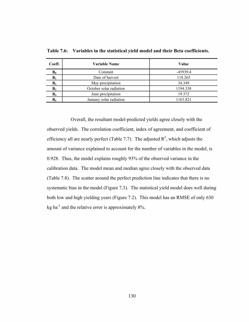
Table 7.6: Variables in the statistical yield model and their Beta coefficients.

Coeff. Variable Name Value

B0 Constant –45939.4 B1 Date of harvest 118.265 B2 May precipitation 34.349 B3 October solar radiation 1194.338 B4 June precipitation 19.372 B5 January solar radiation 1163.821

Overall, the resultant model-predicted yields agree closely with the

observed yields. The correlation coefficient, index of agreement, and coefficient of

efficiency all are nearly perfect (Table 7.7). The adjusted R2, which adjusts the

amount of variance explained to account for the number of variables in the model, is

0.928. Thus, the model explains roughly 93% of the observed variance in the

calibration data. The model mean and median agree closely with the observed data

(Table 7.8). The scatter around the perfect prediction line indicates that there is no

systematic bias in the model (Figure 7.3). The statistical yield model does well during

both low and high yielding years (Figure 7.2). This model has an RMSE of only 630

kg ha-1 and the relative error is approximately 8%.

130

Table 7.7: Model performance statistics for the statistical model during the calibration period [n=14].

Model Performance

Statistic

Statistical Model

RMSE (kg ha-1) 630.83

MAE (kg ha-1) 472.22 Correlation (r) 0.98

D index 0.99 Coefficient of Efficiency (E) 0.96

Table 7.8: Descriptive statistics for observed and statistical model-predicted yield (kg ha-1) [n=14].

Descriptive Statistic Observed Yield Statistical Model

Mean 7908.1 7908.1 Median 8850.5 8850.1

Standard Deviation 3006.7 2939.2

131

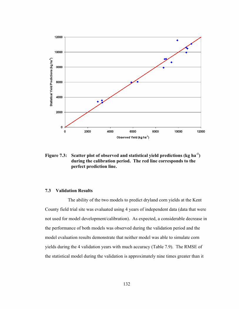
Figure 7.3: Scatter plot of observed and statistical yield predictions (kg ha-1) during the calibration period. The red line corresponds to the perfect prediction line.

7.3 Validation Results

The ability of the two models to predict dryland corn yields at the Kent

County field trial site was evaluated using 4 years of independent data (data that were

not used for model development/calibration). As expected, a considerable decrease in

the performance of both models was observed during the validation period and the

model evaluation results demonstrate that neither model was able to simulate corn

yields during the 4 validation years with much accuracy (Table 7.9). The RMSE of

the statistical model during the validation is approximately nine times greater than it

132

was during the calibration (it increased from 630.83 to 5847.03 kg ha-1). The small

sample size of the calibration data is largely to blame for the inflation of the earlier

model performance statistics. The statistical model predicted corn yields of 17,460 kg

ha-1 in 1989 while actual yields were only 7871 kg ha-1 (Figure 7.4). This extreme

over-prediction of yield (9589 kg ha-1) has a major impact on the model performance

statistics and it accounts for the negative relationship between the observed yields and

those predicted by the statistical model (r = –0.82; D index = 0.11). Even though the

yield deviations during 1990, 1996, and 2000 (2506, 1512, and 1434 kg ha-1

respectively) are much smaller, the coefficient of efficiency indicates that the

statistical model has little predictive power during the validation period.

This large change in model performance between calibration and

validation can be partly attributed to the small number of observations available for

both model calibration and model validation. The model derived from the calibration

data closely fit the observed data because of the large number of parameters in the

model compared to the number of observations (e.g., there were very few degrees of

freedom). Statistical models are also not suited for extrapolating beyond the

conditions under which they were developed. The observed weather conditions in

1989 were significantly different from those in the calibration period and this

produced a large error in the yield predictions. For example, corn is normally planted

at the end of April or the beginning of May but in 1989, it was not planted until May

30. The date of harvest in 1989 was October 26 – the latest harvest to occur between

1984 and 2003. June precipitation was also more than twice the normal amount (228

mm versus 94 mm), greater than any month during the calibration period. May

precipitation and October solar radiation in 1989 were also greater than normal.

133

These positive anomalies in 4 of the 5 independent variables in the yield prediction

model resulted in the extreme over-prediction of yield in 1989.

By contrast, the DSSAT model performed significantly better than the

statistical model during the validation period. The DSSAT model predicted yields

were positively correlated with the observed yields and the RMSE was less than half

of the statistical model (Table 7.9). However, the RMSE increased by approximately

800 kg ha-1 during the validation period and both the index of agreement and

coefficient of efficiency decreased. The DSSAT model was able to closely simulate

corn yields during 1989 (over-predicted by 985 kg ha-1) and 1990 (under-predicted by

482 kg ha-1), but under-predicted yields in 1996 and 2000 (under-predicted by 2936

and 2573 kg ha-1) (Figure 7.4).

Table 7.9: Model performance statistics for both yield models (CERES-Maize and statistical) during the validation period [n=4].

Model Performance

Statistic CERES-Maize Statistical

RMSE (kg ha-1) 2340.98 5847.03

MAE (kg ha-1) 2325.08 5013.45 Correlation (r) 0.62 –0.82

D index 0.63 0.11 Coefficient of Efficiency (E) –0.03 –5.44

134

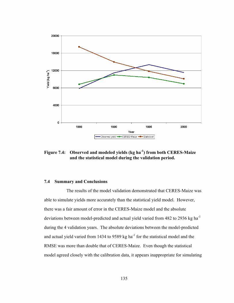
Figure 7.4: Observed and modeled yields (kg ha-1) from both CERES-Maize and the statistical model during the validation period.


The results of the model validation demonstrated that CERES-Maize was

able to simulate yields more accurately than the statistical yield model. However,

there was a fair amount of error in the CERES-Maize model and the absolute

deviations between model-predicted and actual yield varied from 482 to 2936 kg ha-1

during the 4 validation years. The absolute deviations between the model-predicted

and actual yield varied from 1434 to 9589 kg ha-1 for the statistical model and the

RMSE was more than double that of CERES-Maize. Even though the statistical

model agreed closely with the calibration data, it appears inappropriate for simulating

135

yield at the field level. One of the major reasons for the poor performance of the

statistical model during the validation periods is that linear statistical models cannot

be accurately extrapolated beyond the conditions under which they were developed

(e.g., they do a poor job of simulating extreme years). Conditions in 1989 differed

significantly from the years used to calibrate the model, which produced an unrealistic

prediction of yield. Extreme years are of particular interest because for an agricultural

monitoring system to be of value, it must be able to accurately simulate soil moisture

and yield conditions during extreme years. The absolute deviation of the DSSAT

model in 1989 was 985 kg ha-1, roughly one tenth of the statistical model. This

underscores why the DSSAT model is more appropriate to use for field-level

predictions of crop yield. If more calibration data were available the statistical model

might have been able to more accurately model yield, however predictions during

extreme years are always going to be problematic. Another problem with statistical

models is that they are location specific and so the equation developed at the Kent

County field trial site cannot be readily applied in other locations across the state.

Simulation of crop yield is a difficult task because it depends on accurate

simulation of soil water, soil nutrients, diseases, and weeds (Ma et al., 2002). Here,

the models simulated yield based solely on variations in weather conditions, carbon

dioxide concentration, and crop management (e.g., row spacing, seeding density,

seeding depth, date of planting, date of harvest, soil type). The impact of variations in

soil fertility (e.g., fertilizer applications), plant disease, and weeds were not simulated.

Extreme weather events were also not accounted for by CERES-Maize. Discrepancies

between observed and modeled yields may be due to (1) inaccurate soil water and soil

nutrient parameterization, (2) lack of model sensitivity to environmental stress, (3)

136

unrecorded damage from pests, disease, weeds, or extreme weather events, (4)

variability (error) in field measurements, and (5) inability of the model to accurately

simulate crop growth processes.

One of the largest sources of error in the DSSAT model is likely related to

the improper knowledge of soil parameters because detailed soil survey information

was not available for the field trial sites. Therefore, assumptions had to made about

soil type (e.g., the number of the layers, the depth of each layer, and the soil

parameters) based on the information available from the STATSGO soil surveys. As

demonstrated in Chapter 5, yield is sensitive to variations in soil type (and soil

parameters) because yield is highly correlated with soil moisture. Incorrect soil

parameterizations will produce inaccurate yield predictions.

The accuracy of the model results is also negatively impacted by the

accuracy of the weather data. Recent research has demonstrated that relatively small

errors in the measurement of air temperature, precipitation, and solar radiation

(respectively ±0.2°C, ±2%, and ±3%) produce an average error of 5–7% in DSSAT

yield simulations (Fodor and Kovács, 2005). Weather data are not available at the

field trial site, so data from the COOP station in Dover, DE were used instead.

Although the COOP data are relatively accurate, precipitation is highly spatially

heterogeneous, especially during the growing season, and therefore since the gage is

not located at the field trial site, this will likely introduce errors that are greater than

±2%. The errors in solar radiation data are probably larger than those of precipitation

because solar radiation data is being estimated with a model. Overall, the

uncertainties/errors in the weather data are relatively small compared to those in the

137

other input datasets (e.g. soils), but they may still account for a portion of the model

error.

These results are similar to other studies that have validated CERES-

Maize using field trial data. For example, Ma et al. (2002) carried out a 3-year

validation of CERES-Maize in Akron, CO and determined that the RMSE for yield

was 3609 kg ha-1. The RMSE for this validation was 2027 kg ha-1. Anapalli et al.

(2005) also used CERES-Maize to simulate yield and found that the mean error [mean

error = (predicted yield–actual yield)/actual yield] in the yield predictions for the three

different varieties that they tested ranged from 6 to 17%. In this study, the mean error

in the CERES-Maize yield predictions during the 4-year validation was 15%.

The results of the validation study suggest that CERES-Maize can

adequately simulate yield and although there is still a fair amount of error in the yield

predictions (~15%) these results are similar to other validation studies. Much of the

remaining error in the yield predictions can be attributed to errors and uncertainties in

the input data and the inability of CERES-Maize to simulate damage from pests,

disease, weeds, or extreme weather events. In addition, the model-simulated yield for

a single variety was compared to the mean of all the varieties in the early-medium

maturity group (N ranged from 21 to 35 varieties/year) grown at the field trial site.

The collection of additional data at the field trial site (e.g., LAI, ET, silking date,

maturity date, soil moisture data, and detailed soil surveys) would have facilitated a

more detailed model calibration.

138

Chapter 8

EVALUATING THE NEAR-REAL-TIME AGRICULTURAL DROUGHT MONITORING SYSTEM (ADMS)

The ability of the Agricultural Drought Monitoring System (ADMS) to

provide near-real-time predictions of crop yield across Delaware is evaluated using

data from three recent growing seasons (2001, 2002, and 2003). These three years are

particularly useful for evaluating the ADMS because moisture conditions were

extremely varied (as previously discussed in Section 2.4). In this chapter the ADMS

will be evaluated to determine the accuracy of the crop yield predictions and to

establish at what point during the growing season the ADMS yield forecasts attain a

reasonable (useful) amount of accuracy.

8.1 Description of the ADMS Evaluation

The three main elements required to make near-real-time predictions of

crop yield are weather data from the current growing season, predictions of future

weather (e.g., seasonal climate forecasts), and a crop model that is able to simulate the

impact of weather variability on yield.

8.1.1 Weather Data from the Current Growing Season

The ADMS system was evaluated in hindcast mode; that is, the ADMS

was fed weather data from 2001–2003 as if they were real-time data and these data

were used to create the required weather datasets for each of the 224 agricultural grid

139

cells in Delaware. Daily maximum and minimum air temperature data were calculated

by interpolating the observed data from Wilmington, Dover, and Georgetown (2001 to

2003) using an Inverse Distance Weighting (IDW) algorithm (weighting = 1/d2; radius

of influence = 150 km). Daily solar radiation data were calculated with the MH model

based on the daily maximum and minimum air temperatures (as described in Section

4.2). Daily precipitation data were based on radar-derived precipitation estimates

(Section 4.4). The radar data were processed using a gage-radar calibration algorithm

(Legates, 2000). Unfortunately, even after the calibration algorithm was applied the

radar-estimated precipitation was still systematically greater than the observed amount

of precipitation (Tables 8.1, 8.2, and 8.3). The magnitude of this bias ranged from

1.18 (ratio of radar-estimated precipitation to gage precipitation) (Dover, 2002) to

1.48 (Wilmington, 2001). On average, the radar-estimated precipitation was 1.31

times larger than the gage-measured precipitation. An examination of the calibrated

radar precipitation estimates demonstrated that the radar and gage closely agree in

terms of the occurrence of rainfall events, but the radar tends to overestimate the

magnitude of these events (Figure 8.1). The problem may result from the limited

availability of gage observations for calibration (Legates, personal communication,

April 20, 2005). All of the calibrated radar precipitation estimates (2001–2003) were

adjusted for the remaining bias by dividing the precipitation estimates by 1.31 (the

mean radar/gage bias based on the data in Tables 8.1, 8.2, and 8.3). In addition,

between April 29 and May 28, 2002, data from the radar at Sterling, VA (KLWX) was

unavailable. Therefore, calibrated radar precipitation estimates for these 23 days use

only the radar data from Dover AFB, DE (KDOX) and Mt. Holly, NJ (KDIX).

140

Table 8.1: Gage-measured and radar-estimated precipitation at Dover (April 1 to October 31, 2001–2003).

Year Gage-measured

Precipitation (mm)

Radar-estimated Precipitation

(mm)

Radar/Gage Precipitation

2001 597.3 710.5 1.19 2002 819.8 964.8 1.18 2003 968.8 1243.8 1.28

Table 8.2: Gage-measured and radar-estimated precipitation at Wilmington (April 1 to October 31, 2001–2003).

Year Gage-measured

Precipitation (mm)


(mm)


2001 483.8 717.8 1.48 2002 590.8 872.0 1.47 2003 882.0 1149.0 1.30

Table 8.3: Gage-measured and radar-estimated precipitation at Greenwood (April 1 to October 31, 2002–2003) [gage data are missing in August 2001].

Year Gage-measured

Precipitation (mm)


(mm)


2001 - - - 2002 807.5 1041.2 1.29 2003 884.0 1144.8 1.29

141

Figure 8.1: Gage-measured and radar-estimated precipitation at Georgetown

(April 1 to July 19, 2001).

All days that had more than 76.2 mm (3 in.) of radar-estimated

precipitation were individually examined and verified (Table 8.4). A number of errors

were identified and subsequently corrected through this analysis. On July 22, 2002,

the radar-estimated precipitation at Wilmington was 188 mm, however all gages

recorded 0 mm of precipitation. Therefore, it was assumed that the radar was in error

and the precipitation for July 22, 2002 was set to 0 mm. A problem with radar data

was also detected on September 11, 2002. The radar estimated that 80 mm of

precipitation occurred in Wilmington, but none was recorded by the gage. Therefore,

the precipitation for September 11, 2002 was also set to 0 mm.

142

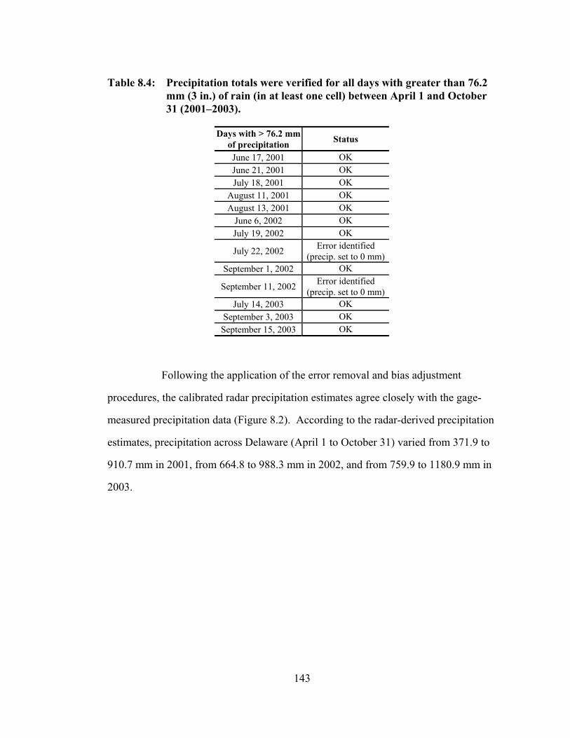
Table 8.4: Precipitation totals were verified for all days with greater than 76.2 mm (3 in.) of rain (in at least one cell) between April 1 and October 31 (2001–2003).

Days with > 76.2 mm of precipitation Status

June 17, 2001 OK June 21, 2001 OK July 18, 2001 OK

August 11, 2001 OK August 13, 2001 OK

June 6, 2002 OK July 19, 2002 OK

July 22, 2002 Error identified (precip. set to 0 mm)

September 1, 2002 OK

September 11, 2002 Error identified (precip. set to 0 mm)

July 14, 2003 OK September 3, 2003 OK

September 15, 2003 OK

Following the application of the error removal and bias adjustment

procedures, the calibrated radar precipitation estimates agree closely with the gage-

measured precipitation data (Figure 8.2). According to the radar-derived precipitation

estimates, precipitation across Delaware (April 1 to October 31) varied from 371.9 to

910.7 mm in 2001, from 664.8 to 988.3 mm in 2002, and from 759.9 to 1180.9 mm in

2003.

143

Figure 8.2: Gage-measured versus bias-adjusted radar-estimated precipitation (mm). The points on the graph correspond to the stations listed in Tables 8.1, 8.2, and 8.3. The red line is the perfect prediction line.

8.1.2 Prognostications of Future Weather

Estimates of future weather conditions can be obtained using a number of

approaches. One approach is to use historical data or climatology (Duchon, 1986).

Climatological (mean) values can be calculated based on the historical data and used

to represent weather conditions during the remainder of the growing season.

However, the use of mean values is less than satisfactory because it eliminates much

of the variability that is normally associated with growing season weather conditions.

An alternative approach is to search the historical record for a similar year (historical

144

analogue). Data from this analogue year can then be used to represent weather

conditions during the remainder of the growing season. An obvious drawback of this

approach is that no two growing seasons are identical, and current weather conditions

do not necessarily dictate future weather conditions. Therefore, the best approach for

using the historical data is to select a number of years of historical data and run the

model for each, thus producing a range of possible outcomes. This range of yield

predictions can be used to determine a mean yield prediction and to estimate the

probability/uncertainty associated with each yield prediction (Chipanshi et al., 1997).

Another approach is to use weather simulators (generators) to create

hypothetical weather data that adheres to the known statistical properties of weather

conditions at a particular location (Bannayan et al., 2003; Jagtap and Jones, 2002).

However, historical data are more appropriate than statistically generated (artificial)

weather data since they represent the appropriate inter-correlations between weather

variables (Chipanshi et al., 1997). Therefore, historical data will be used for making

yield predictions.

Historical data were generated following the same methodology used to

construct the ‘real time’ data, except that precipitation data was derived from gage

data during the historical period (1971–2000). All missing air temperature and

precipitation data were filled, prior to the interpolation, using data from the closest

active meteorological station (Tables 8.5, 8.6, and 8.7). Daily maximum and

minimum air temperature and precipitation data were calculated by interpolating the

observed data from Wilmington, Dover, and Georgetown. Daily solar radiation data

were calculated for each grid cell with the Mahmood-Hubbard model using the daily

maximum and minimum air temperatures (as described in Section 4.2).

145

Table 8.5: Number of days with missing maximum and minimum air temperature and precipitation data at Wilmington (1971–2003)

Year Maximum Temp.

Minimum Temp. Precip. Station Used to Replace Missing Data

2003 0 0 0 -- 2002 0 0 0 -- 2001 0 0 0 -- 2000 0 0 1 Newark 1999 1 0 0 Newark 1998 2 1 0 Newark 1997 0 6 58 Newark 1996 0 11 151 Newark 1995 0 5 61 Newark 1994 0 0 0 -- 1993 0 0 0 -- 1992 0 0 0 -- 1991 0 0 0 -- 1990 0 0 0 -- 1989 0 0 0 -- 1988 0 0 0 -- 1987 0 0 0 -- 1986 0 0 0 -- 1985 0 0 0 -- 1984 0 0 0 -- 1983 0 0 0 -- 1982 0 0 0 -- 1981 0 0 0 -- 1980 0 0 0 -- 1979 0 0 0 -- 1978 0 0 0 -- 1977 0 0 0 -- 1976 0 0 0 -- 1975 0 0 0 -- 1974 0 0 0 -- 1973 0 0 0 -- 1972 0 0 0 -- 1971 0 0 0 --

146

Table 8.6: Number of days with missing maximum and minimum air temperature and precipitation data at Dover (1971–1983) (remainder of the missing data for Dover (1984–2003) is shown in Table 4.4)

Year Maximum Temp.


1983 0 0 0 -- 1982 0 0 1 Milford 2SE 1981 0 0 0 -- 1980 31 32 31 Milford 2SE 1979 31 31 31 Milford 2SE 1978 0 0 0 -- 1977 0 0 0 -- 1976 0 0 0 -- 1975 0 1 0 Milford 2SE 1974 0 2 0 Milford 2SE 1973 31 31 31 Milford 2SE 1972 0 0 0 -- 1971 0 0 0 --

Table 8.7: Number of days with missing maximum and minimum air temperature and precipitation data at Georgetown (1971–1983) (remainder of the missing data for Georgetown (1984–2003) is shown in Table 4.2)

Year Maximum Temp.


1983 0 0 3 Milford 2SE 1982 0 0 16 Milford 2SE 1981 0 0 9 Milford 2SE 1980 0 0 9 Milford 2SE 1979 1 1 4 Milford 2SE 1978 0 0 4 Milford 2SE 1977 0 0 5 Milford 2SE 1976 1 5 8 Milford 2SE 1975 1 4 9 Milford 2SE 1974 0 4 13 Milford 2SE 1973 1 1 12 Milford 2SE 1972 0 0 20 Milford 2SE 1971 0 0 4 Milford 2SE

147

8.1.3 Simulating Yield in Near-Real-Time

Yield forecasts were prepared for four different forecast dates (June 1,

July 1, August 1, and September 1) in each growing season (2001, 2002, and 2003).

For each forecast date, the observed weather data were used up to the day of the

forecast and historical data were used from the time of the forecast until harvest.

Thus, thirty different simulations (one for each year of historical data) were carried

out at each grid point for each forecast date, in total 80,640 separate model runs were

completed (3 years x 4 forecast dates/year x 30 simulations/forecast date x 224 grid

cells = 80,640 simulations).

Field trial reports were used to define all of the required model parameters

(e.g., row spacing, seeding density, seeding depth, date of planting, date of harvest).

Each model run was performed using the identical crop and management conditions

(Table 8.8) and only the weather data and soil type were allowed to vary from one grid

cell to another. Thus, all of the model-simulated interannual variations in yield are

due to the weather conditions and soil type.

Table 8.8: CERES-Maize model parameters used for the ADMS simulations

Model Parameter Value

Row spacing (cm) 75 Seeding Density (plants/cm) 7

Seeding Depth (cm) 5 Cultivar SQ6192 (coefficients are listed in Table 7.3)

CO2 Concentration (ppm) 376 Start of Simulation April 1 (JD 91) End of Simulation October 31 (JD304)

Seeding Date May 1 (JD 121) Harvest Date October 1 (JD 274)

Initial Soil Moisture 70% of field capacity

148

8.2 Results of the ADMS Evaluation: Assessing ADMS Accuracy

The ability of the ADMS to model crop yield in Delaware was assessed by

comparing the model-predicted State yield with the observed State yield during 2001–

2003. The observed (or ‘real-time’) weather data was used to simulate corn yield at

all agricultural grid cells (2001–2003). The mean model-predicted State yield for each

year was determined by first averaging the yield predictions for all grid cells within

each county (New Castle = 34; Kent = 75; Sussex = 115). Then, the mean yield for

Delaware was calculated by multiplying the mean yield for each county by the

percentage that it contributes to the corn harvest (based on the number of acres

harvested in each county during 2001–2003) (Table 8.9). This method was used

rather than basing the calculation on an area-weighted average (e.g., the number of

agricultural grid cells in each county) because there was no way of verifying what

type of agricultural activity (if any) took place at the cells identified as agricultural

from the LULC data. Weighting the counties by area (New Castle = 15.2%; Kent =

33.5%; Sussex = 51.3%) gives a different answer than if the county weights are

determined by production (New Castle = 12.1%; Kent = 24.2%; Sussex = 63.7%). For

example, based on the amount of agricultural area in Kent County (e.g., number of

grid cells designated as agricultural) it should account for 33.5% of the corn

production in Delaware, however in reality corn production in Kent County only

accounts for 24.2% of the total corn production. Therefore, a production-weighted

method was used to avoid giving too much weight to yields in New Castle and Kent

counties.

Model-predicted State yields systematically over-estimate the observed

yields in Delaware (Table 8.10). Similar findings have been observed in other studies

where crop simulation models have been used to determine regional yields (Chipanshi

149

et al., 1999; Jagtap and Jones, 2002). Yield models tend to systematically over-

estimate regional yields because they generally do not account for yield reductions

due to outbreaks of disease, pests, and extreme weather events (e.g., wind damage). In

addition, soil fertility was not accounted for in this simulation. Therefore, a bias

adjustment was applied to all of the state yield estimates (divide by 1.15) following

Jagtap and Jones (2002). This bias adjustment is meant to account for the yield

stresses that are not included in the model. This bias adjustment factor appears to be

fairly stable during 2001–2003, which suggests that reductions in yield caused by

factors such as disease, pests, and soil fertility remain relatively constant from year to

year, at least when considered at the state (regional) level.

Table 8.9: Mean corn production in Delaware by county (2001–2003)

County Production (acres) Percentage of Total Production

New Castle 20,000 12.1% Kent 40,000 24.2%

Sussex 105,000 63.7% Total 165,000 100%

Table 8.10: Observed and model-predicted mean corn yield in Delaware (2001–2003)

Year Observed Yield (kg ha-1)

Model-predicted Yield (kg ha-1)

Ratio of Model-predicted to

Observed Yield

Bias-adjusted Model-predicted

Yield (kg ha-1)

Observed – Bias-adjusted

(kg ha-1) 2001 9164 10,486 1.14 9198 –34 2002 5210 5920 1.14 5148 –62 2003 8223 9523 1.16 8281 2 Mean 7532 8643 1.15 7542 –31

150

After applying the bias adjustment to the model-predicted State yields, the

modeled and observed yields agree extremely well. The difference between the yields

varies from 2 to 62 kg ha-1, an error of less than 1%. It is particularly noteworthy that

the model is able to correctly predict yield during all three years since they had such

varied growing-season weather conditions. In 2001, corn yields in Delaware were

significantly above average (9164 kg ha-1 compared to an average (1990–2003) of

7206 kg ha-1). Although precipitation was below normal during April, September, and

October of 2001 in both northern (Table 8.11) and southern Delaware (Table 8.12),

precipitation was favorable during the growing season months (May through August),

resulting in above average corn yields. In 2002, corn yields were significantly below

average (5210 kg ha-1 compared to an average (1990–2003) of 7206 kg ha-1).

Precipitation was below normal in June, July, and August in southern Delaware (July

and August in northern Delaware). This lack of precipitation during the critical

growth phases resulted in corn yields that were well below average. Conditions at the

end of the 2002 growing season were significantly wetter than normal, but

unfortunately this rain occurred too late to help the corn crops. The 2003 growing

season was much wetter than normal. Large amounts of precipitation fell during June

and September in northern Delaware and conditions were also wetter than normal

from April to October in southern Delaware. These extremely wet conditions resulted

in slightly higher than normal yields (8223 kg ha-1 compared to an average (1990–

2003) of 7206 kg ha-1), however the cool, wet conditions prevented yields from

reaching 2001 levels. Despite the varied moisture conditions, model-predicted yields

were extremely accurate during all three years. Therefore it can be concluded that the

ADMS is a suitable tool for monitoring state corn yields.

151

Table 8.11: April to October (2001–2003) Standardized Precipitation Index (SPI) values in northern Delaware (Climate Division 1)

Month 2001 2002 2003

April –1.38 –0.40 –0.38 May 0.78 0.38 0.29 June 0.44 0.29 2.92 July –0.95 –1.33 –0.81

August 0.20 –1.08 0.95 September –0.17 0.21 2.01

October –1.64 1.80 1.25

Table 8.12: April to October (2001–2003) Standardized Precipitation Index (SPI) values in southern Delaware (Climate Division 2)

Month 2001 2002 2003

April –1.32 0.77 0.24 May –0.05 0.04 0.95 June 1.36 –0.46 1.55 July 0.90 –0.48 0.73

August 0.59 –0.46 0.34 September –0.77 1.72 1.12

October –1.34 2.24 0.42

8.3 Results of ADMS Evaluation: Forecasting Accuracy

Since the ADMS can accurately simulate Delaware corn yields using

observed weather data, the predictive abilities of the model will be examined to

determine when the model attains a reasonable amount of forecast accuracy. The

ability of the ADMS to forecast corn yields will be assessed by validating the model

forecasts using the results from the full season model simulations. This is a

reasonable method for evaluating the forecasting accuracy of the ADMS in light of the

lack of high-resolution yield data and given the ability of the ADMS to accurately

simulate State yields.

152

8.3.1 Forecasting Accuracy in 2001

The first yield forecast is made on June 1 (30 days after planting) and, as

expected, this forecast is the least accurate (Table 8.12). The predicted mean based on

the June 1 forecast significantly underestimates the observed yield. It is important to

note that the mean yields in this section are not the same as the state-level yield

estimates discussed in Section 8.2 because they represent the unweighted averages and

no bias adjustements have been applied. In addition, the error statistics (RMSE,

MAE, and mean percent error (MPE)) are all quite large and the goodness-of-fit

statistics (r2, D, and E) are all quite small. By the second yield forecast on July 1 (61

days after planting), the predicted yield has increased and the amount of error has

decreased. However, even though the MPE is less than 15%, the goodness-of-fit

statistics indicate that the model predictions do not accurately capture the observed

spatial pattern of yield variability. However, by the third forecast on August 1 (92

days after planting) there has been a significant improvement in the model’s accuracy.

The mean predicted yield (10,616 kg ha-1) is very similar to the observed yield

(10,387 kg ha-1) and the error statistics are roughly one third of what they were during

the previous forecast. The MPE is less than 5%, suggesting that a relatively accurate

yield forecast could be made on August 1. Roughly 75% of the variance in the

observed yield is accounted for by the August 1 forecast. The other goodness-of-fit

statistics (D = 0.92 and E = 0.69) also highlight the predictive power of the August 1

forecast. The fourth and final yield forecast is made on September 1 (123 days after

planting) and naturally it is even more accurate than the preceding three. This is

partly because, by September 1, the crop has reached maturity at many of the locations

across Delaware and therefore subsequent weather variations will have little impact on

yield. Thus, it is not surprising to find that the September 1 yield forecast is able to

153

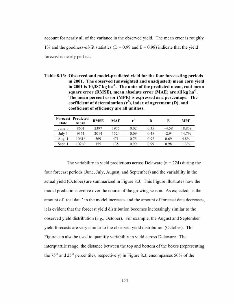
account for nearly all of the variance in the observed yield. The mean error is roughly

1% and the goodness-of-fit statistics (D = 0.99 and E = 0.98) indicate that the yield

forecast is nearly perfect.

Table 8.13: Observed and model-predicted yield for the four forecasting periods in 2001. The observed (unweighted and unadjusted) mean corn yield in 2001 is 10,387 kg ha-1. The units of the predicted mean, root mean square error (RMSE), mean absolute error (MAE) are all kg ha-1. The mean percent error (MPE) is expressed as a percentage. The coefficient of determination (r2), index of agreement (D), and coefficient of efficiency are all unitless.

Forecast Date

Predicted Mean RMSE MAE r2 D E MPE

June 1 8601 2397 1975 0.02 0.35 –4.58 18.8% July 1 9351 2014 1524 0.09 0.48 –2.94 14.7% Aug. 1 10616 569 471 0.75 0.92 0.69 4.8% Sept. 1 10269 155 135 0.99 0.99 0.98 1.3%

The variability in yield predictions across Delaware (n = 224) during the

four forecast periods (June, July, August, and September) and the variability in the

actual yield (October) are summarized in Figure 8.3. This Figure illustrates how the

model predictions evolve over the course of the growing season. As expected, as the

amount of ‘real data’ in the model increases and the amount of forecast data decreases,

it is evident that the forecast yield distribution becomes increasingly similar to the

observed yield distribution (e.g., October). For example, the August and September

yield forecasts are very similar to the observed yield distribution (October). This

Figure can also be used to quantify variability in yield across Delaware. The

interquartile range, the distance between the top and bottom of the boxes (representing

the 75th and 25th percentiles, respectively) in Figure 8.3, encompasses 50% of the

154

predicted yield distribution. Therefore, the length of the box represents the amount of

spatial heterogeneity in yield predictions across Delaware. Both the June and July

yield forecasts show a great deal of spatial heterogeneity in yield predictions across

the state. By August, the interquartile range has significantly decreased, indicating

that there is much less spatial heterogeneity in yield predictions across the state.

However, the long whiskers for the August, September, and October boxes indicate

that very low yields occurred at a few locations in Delaware. It is likely that the areas

of low yield correspond to the areas of low precipitation. For example, precipitation in

Delaware (April 1 to October 31) varied from 371.9 to 910.7 mm in 2001.

Since 30 model simulations are performed for each grid cell at each of the

four forecast dates, it is possible to use the range of yield predictions to calculate the

probability of obtaining a given yield (Figure 8.4). Because the yield forecasts are

most uncertain at the beginning of the growing season, the probability curves are the

steepest for the early forecast dates (e.g., June and July). However, as the growing

season progresses, the probability curves become flatter, indicating that there is less

uncertainty in the yield predictions. For example, based on the June 1 forecast, there

is a 50% chance that the observed yield will be between 7035 and 9864 kg ha-1 and

based on the July 1 forecast, a 50% chance exists that the observed yield will be

between 8189 and 10,283 kg ha-1. By August, there is a 50% chance that the observed

yield will be between 9928 and 11,378 kg ha-1. This narrower range in yields

indicates that the forecast accuracy has improved somewhat. Based on the September

yield forecast, a 50% chance exists that the observed yield will be between 10,060 and

10,475 kg ha-1. The observed state yield in 2001 was 10,387 kg ha-1, which falls

within the August and September 50% forecast thresholds (and it is just outside of the

155

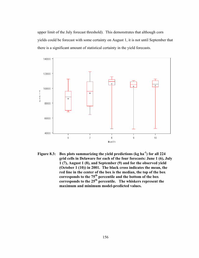
upper limit of the July forecast threshold). This demonstrates that although corn

yields could be forecast with some certainty on August 1, it is not until September that

there is a significant amount of statistical certainty in the yield forecasts.

Figure 8.3: Box plots summarizing the yield predictions (kg ha-1) for all 224 grid cells in Delaware for each of the four forecasts: June 1 (6), July 1 (7), August 1 (8), and September (9) and for the observed yield (October 1 (10)) in 2001. The black cross indicates the mean, the red line in the center of the box is the median, the top of the box corresponds to the 75th percentile and the bottom of the box corresponds to the 25th percentile. The whiskers represent the maximum and minimum model-predicted values.

156

Figure 8.4: Model-predicted exceedance probabilities (%) for State corn yield based on the June 1, July 1, August 1, and September 1 forecasts in 2001


The results from 2002 differ significantly from 2001. The predicted mean

based on the June 1 forecast significantly overestimates the observed yield in 2002

(Table 8.13). The RMSE and MAE are much higher during the June 2002 yield

forecast compared to the June 2001 forecast (RMSE is 766 kg ha-1 larger, MAE is 959

kg ha-1 larger, and the MPE is approximately 43% greater). Despite the inflated error

statistics, the goodness-of-fit statistics (r2, D, and E) all indicate that the June 2002

forecast more closely approximate the observed data than the June 2001 forecast.

157

This suggests that although the model does not correctly predict the magnitude of the

yield, it correctly predicts the spatial pattern (i.e., the model is predicting higher and

lower yields in the correct locations). The second yield forecast on July 1 is similar to

the first. The model-predicted yield significantly overestimates the observed yield and

the error statistics are just as large as they were in the June forecast. The goodness-of-

fit statistics are also relatively similar to the June forecast. Based on these results, it

can be concluded that it is not possible to make accurate yield predictions at this point

in the growing season. By the third forecast on August 1, some improvement in the

model’s accuracy has been observed, although the mean predicted yield (8430 kg ha-1)

is almost 2400 kg ha-1 greater than the observed yield. The error statistics have

decreased in comparison to the second forecast period and the goodness-of-fit

statistics have increased. Based on the coefficient of determination, roughly 87% of

the variance in the observed yield is accounted for by the August 1 yield forecast,

however the MPE is still nearly 47%, which suggests that a relatively accurate yield

forecast is not possible on August 1. The poor performance in June, July, and August

is partially due to the unique weather conditions (i.e., hot dry summer) in 2002. The

fourth yield forecast on September 1 finally shows close correspondence with the

observed yield. The goodness-of-fit statistics indicate that the model is able to

perfectly predict yield at all locations. The main reason for this sudden jump in the

model performance statistics is that by September 1 the crop has reached maturity at

most locations across Delaware. Thus, subsequent weather variations have little

impact on yield.

158

Table 8.14: Observed and model-predicted yield for the four forecasting periods in 2002. The observed (unweighted and unadjusted) mean corn yield in 2002 is 6044 kg ha-1.

Forecast Date


June 1 8950 3163 2934 0.68 0.61 –1.23 62.2% July 1 9323 3468 3308 0.74 0.61 –1.68 65.8% Aug. 1 8430 2514 2407 0.87 0.74 –0.41 46.7% Sept. 1 6030 56 29 1.0 1.0 1.0 0.5%

Since 2002 was a relatively unique event, at least in the last 30 years,

the ADMS was not able to accurately predict yields because the historical record

contains no suitable analogues for this growing season. Therefore, the model-

predicted yields consistently overestimated yield until September (Figure 8.5). In

2002, the spatial heterogeneity in yield predictions were much greater than in 2001.

Unlike 2001, the interquartile range does not decrease as the growing season

progresses. This suggests that conditions were not only drier in 2002, but there was

also significant spatial variability in precipitation across the state.

159

Figure 8.5: Box plots summarizing the forecast yield (kg ha-1) for all 224 grid cells for each of the four forecasts (June 1, July 1, August 1, and September 1) and for the observed yield (October 1) in 2002.

The model-predicted yield probabilities for each of the four forecast dates

in 2002 are shown Figure 8.6. The probability curves for June and July are quite

similar and both are relatively steep. This indicates that there is very little certainty in

the yield data at this point in the growing season. The interquartile range for June and

July are 2407 and 2094 kg ha-1, respectively. Based on the June 1 forecast there is a

50% chance that the observed yield will be between 7673 and 10,080 kg ha-1 and for

the July 1 forecast there is a 50% chance that the observed yield will be between 8214

and 10,380 kg ha-1. These two probability curves are quantitatively very similar to the

June and July probability curves for 2001. This is not surprising given the majority of

160

data used to construct both these curves is based on the historical record, since it is

relatively early in the growing season. In August, the interquartile range is less than

half of what it was in June and July and there is a 50% chance that the observed yield

will be between 8097 and 9087 kg ha-1. Based on the last forecast in September, there

is a 50% change that the observed yield will be between 5998 and 6048 kg ha-1. The

crop yield can be predicted with such certainty by September that the probability line

is nearly flat. The observed mean yield for Delaware in 2002 (6044 kg ha-1) only falls

between the 50% forecast thresholds in September, indicating that corn yield could not

be accurately predicted by the model prior to September 1.


161


The results from 2003 are quite similar to the results from 2001. Both

years produced above average yields and both show similarity in the timing and

magnitude of forecast accuracy. The predicted mean based on the June 1 forecast

closely approximates the observed yield in 2003 (Table 8.13). The RMSE, MAE and

MPE are smaller than in the first forecast for the other two years. For example, the

MPE is only 15.9% for the June 1 forecast in 2003 as compared to 62.2% in 2002 and

18.8% in 2001. However, despite the smaller amount of error in the model

predictions, the goodness-of-fit statistics (r2, D, and E) all indicate that the model does

not correctly predict the spatial pattern (e.g., the model is not predicting higher and

lower yields in the correct locations), which is the exact opposite of what happened in

2002. The July 1 yield forecast is similar to the June 1 forecast, except that the

amount of error in the yield predictions actually increases. In July, the model slightly

overestimated yield.

By the August 1 forecast, some improvement was observed in the

accuracy of the model. Although the mean predicted yield (10,491 kg ha-1) is further

from the observed yield than it was during the June and July forecasts, the amount of

error in the model has decreased. Specifically, the MPE is only 10.4% in August and

the RMSE and MAE have also significantly decreased. However, the goodness-of-fit

statistics still indicate that the model cannot correctly predict the spatial pattern of the

yields. There is a close correspondence between the observed and model-predicted

yield based on the September 1 yield forecast. All of the error statistics decreased in

the September forecast and all of the goodness-of-fit statistics increased. However, it

is interesting to note that despite the fact that the September 1 yield forecast has a

MPE of only 1.2% and an RMSE of 134 kg ha-1, the coefficient of determination is

162

only 0.36 and the coefficient of efficiency is only 0.14. These low values indicate that

even in September, the model cannot correctly resolve the spatial pattern of yield

variation.

Part of the reason for these low values may be because yields were

relatively homogeneous across Delaware. Therefore small differences between the

predicted and observed yields at each grid point could result in low values for the

goodness-of-fit statistics. The State yield in 2003 was accurately predicted by the

June 1 forecast (just 30 days after planting). However, this may be more fortuitous

than an indication of efficacy.

Table 8.15: Observed and model-predicted yield for the four forecasting periods in 2003. The observed mean corn yield (unadjusted) in 2003 is 9505 kg ha-1.

Forecast Date


June 1 9652 1692 1532 0.02 0.08 –135.4 15.9% July 1 9875 1831 1719 0.04 0.07 –158.7 17.9% Aug. 1 10491 1056 995 0.01 0.17 –52.1 10.4% Sept. 1 9437 134 111 0.36 0.69 0.14 1.2%

The spatial heterogeneity in yield predictions during the four forecast

periods and the spatial heterogeneity in the actual yield are summarized in Figure 8.7.

These box plots show a significant amount of spatial heterogeneity in the June and

July yield forecasts. As the amount of ‘real data’ in the model increased, the amount

of heterogeneity in the yield forecasts decreased and the distributions became

increasingly similar to the observed yield. The short whiskers on the August,

September, and October boxes indicate that yields were relatively homogeneous

163

across the state. This is likely due to the ample precipitation that fell across the state

in 2003. According to the radar-derived precipitation estimates, precipitation in

Delaware (April 1 to October 31) varied from 759.9 to 1180.9 mm.

The model-predicted yield probabilities for each of the four forecast dates

in 2003 are shown Figure 8.8. The probability curves for June and July are quite

similar and both are relatively steep. This indicates little certainty in the yield data at

this point in the growing season. The quartile range for June and July are 2338 and

2667 kg ha-1, respectively. Based on the June 1 forecast, a 50% chance exists that the

observed yield will be between 8423 and 10,761 kg ha-1 and for the July 1 forecast,

there is a 50% chance that the observed yield will be between 8296 and 10,963 kg ha-

1. In August, the interquartile range is much smaller than in June and July and there is

a 50% chance that the observed yield will be between 9848 and 11,286 kg ha-1. Based

on the September forecast, a 50% chance that the observed yield will be between 9148

and 9733 kg ha-1. The September probability line in 2003 has a slope that is similar to

the September probability line in 2001. These lines are not as flat as in 2002, which

suggests that crop yield cannot be predicted as accurately. The observed mean yield

for Delaware in 2003 (9505 kg ha-1) falls within the 50% forecast thresholds in June,

July, and September, which suggests that corn yield in 2003 could have been predicted

with limited accuracy as early as June 1.

164

Figure 8.7: Box plots summarizing the forecast yield (kg ha-1) for all 224 grid cells for each of the four forecasts (June 1, July 1, August 1, and September 1) and for the observed yield (October 1) in 2003.

165



Results of the ADMS model evaluation demonstrate that corn yields

across Delaware can be accurately simulated with CERES-Maize using observed

weather data. However, a bias exists that arises from the inability of the crop yield

model to account for yield reductions due to disease outbreaks, pests, and the effect of

extreme weather events (i.e., wind damage). This systematic over-estimation of

regional (state) yields is not unique to the ADMS. Other studies that have performed

crop-model simulations of regional yields report similar findings (Chipanshi et al.,

1999; Jagtap and Jones, 2002). It is encouraging, however, that this bias adjustment

166

appears to be fairly stable during 2001–2003, which suggests that the factors

responsible for reducing yield (e.g., soil fertility) are relatively constant from year to

year, at least when considered at the state (regional) level. After applying the bias

adjustment to the model-predicted state yields, the difference between the model-

predicted and observed state yields varied from 2 to 62 kg ha-1, an error of less than

1%. The ability of the ADMS to correctly predict state yields is especially promising

given the varied growing-season weather conditions in 2001, 2002, and 2003. This

suggests that the ADMS is sensitive enough to variations in observed weather

conditions that it can be used to accurately simulate State yields during all growing

seasons (no matter how extreme).

The ability of the ADMS to forecast corn yields, from one to four months

prior to harvest, was assessed by making four forecasts during each growing season

(June 1, July 1, August 1, and September 1) and validating these forecasts using the

results from the full season model simulations. It is difficult to draw general

conclusions about the forecast accuracy of the ADMS because it varied significantly

from year to year. The results of the forecast evaluation also varied depending on the

statistic used to assess forecast accuracy (e.g., RMSE, MAE, MPE, r2, D, E).

Not surprisingly, forecasts later in the growing season were more accurate

than the forecasts earlier in the growing season because they were based on more

actual data (and less ‘forecast’ data). None of the June 1 yield forecasts were very

accurate. However, the June forecast in 2003 was within 147 kg ha-1 and the MPE

was only 15.9%. Unfortunately, even though the June forecast proved to be relatively

accurate, not much certainty could be placed in it because the confidence bounds

(based on the probability curve) were extremely wide.

167

The July 1 yield forecasts roughly correspond to when the corn crop has

completed the silking stage of development. The RMSE in July ranged from 1831 to

3468 kg ha-1 and the MPE ranged from 14.7% to 65.8%. This indicates that July

forecasts are quite uncertain. Based on the three years of data that were used to assess

the forecast accuracy of the ADMS, it appears that both the June and July forecasts

would be of little value to decision makers because they are too uncertain. However,

it may be possible to improve the early-season yield predictions by utilizing seasonal

climate forecasts to narrow the range of potential weather scenarios that are used to

make the yield predictions.

The August 1 yield forecasts (92 days after planting) roughly correspond

to the middle of the grain fill stage. Yield forecasts in August hold much more

promise than the earlier forecast periods. The RMSE in August ranged from 569 to

2514 kg ha-1 and the MPE ranged from 4.8% to 46.6%. In 2001 the August forecast

was within 229 kg ha-1 of the observed yield, the MPE was only 4.8%, and the

goodness-of-fit statistics also indicate good agreement between the predicted and

observed yield. However, the August 2002 forecast had a large amount of error, even

though it is able to accurately predict the spatial pattern. Since, climatically, 2002 was

a quite unique event, at least in the last 30 years, the model consistently overestimated

yields until the September forecast. The August 2003 forecast was less accurate than

the August 2001 forecast, but more accurate than the August 2002 forecast.

All of the September yield forecasts were extremely accurate. This is not

surprising given that the crop has normally reached maturity by September 1 and

therefore subsequent weather variability has no impact on yield. The RMSE of the

168

September forecasts ranged from 56 to 155 kg ha-1 and the MPE ranged from 0.5% to

1.3%.

Based on these results it can be concluded that it is difficult to make an

accurate yield forecast early in the growing season. In two of the three years,

reasonably accurate yield forecasts could be made starting August 1. In all years it

was possible for the ADMS to accurately simulate yields by September 1. This holds

little value as a forecasting tool because it is too late in the season to make operational

decisions that will have any impact on yield. However, the ADMS may be useful to

state (or federal) agencies that are interested in having accurate yield estimates prior to

harvest. The ADMS can also be used to understand the spatial variability of yield

across the state.

169

Chapter 9

SUMMARY AND CONCLUSIONS

9.1 Summary of Results

The goal of this research was to develop and validate a methodology for

creating a near-real-time Agricultural Drought Monitoring System (ADMS) for

Delaware. Specifically, the primary objectives of this research were (1) to compare a

physiological crop model (CERES-Maize) with a statistical crop model to determine

which is most appropriate for predicting corn yield in Delaware, (2) analyze the

sensitivity of CERES-Maize to determine how uncertainty in the input data affects the

model, (3) validate the soil moisture component of CERES-Maize, and (4) test the

near-real-time ADMS.

The results of the crop model validation demonstrated that CERES-Maize

was able to simulate yields at the field level more accurately than the statistical yield

model. Although the statistical model agreed closely with the calibration data, it is

inappropriate for simulating yield at the field level because linear statistical models

cannot be accurately extrapolated beyond the environmental conditions (e.g., weather,

soil) under which they were developed (e.g., they cannot accurately simulate extreme

years). Agricultural monitoring systems must accurately predict yield during extreme

years since that is when they will be most frequently utilized. Statistical models are

also location specific and so the equations that are developed for one location cannot

be readily applied to other locations.

170

Although the yield predictions made with CERES-Maize during the field

trial validation were more accurate than the statistical model, a fair amount of error in

the yield predictions (~15%) still exists. Absolute deviations between model-

predicted and actual yield varied from 482 to 2936 kg ha-1. These results are similar

to other studies that have validated CERES-Maize using field trial data (Anapalli et

al., 2005; Ma et al., 2002). Discrepancies between observed and modeled yields may

result from inaccurate soil water and nutrient parameterization, lack of model

sensitivity to environmental stress, unrecorded damage from pests, disease, weeds, or

extreme weather events, variability (error) in field measurements, and inability of the

model to accurately simulate crop growth processes. Of these, the largest source of

error is likely related to the improper knowledge of soil parameters. Yield is sensitive

to variations in soil type because soil type determines soil moisture. The collection of

additional data at the field trial site (e.g., LAI, ET, silking date, maturity date, soil

moisture data, and detailed soil surveys) would have facilitated a more detailed model

calibration and potentially more accurate yields predictions.

The sensitivity of CERES-Maize to variations in row spacing, planting

density, planting date, initial soil moisture, carbon dioxide concentration, air

temperature, solar radiation, and soil type was quantified. As row spacing increases

and planting density decreases, yields generally decrease, as expected. However,

CERES-Maize is not overly sensitive to row spacing or planting density, at least not

over the range of values normally encountered in Delaware. Planting date also did not

have a large impact on yield during most years, although it did impact yield during

years when precipitation was unequally distributed throughout the growing season.

This is because the timing of dry spells in relation to the growth stage of the crop is

171

important. Air temperature and planting date both had a similar (non-linear) impact

on yield because both affect the timing of crop growth. Air temperature directly

controls the rate of crop growth and therefore changes in air temperature affect the

duration and timing of the growth stages. Changes in air temperature/planting date

have the largest impact on yield during years when precipitation is unequally

distributed throughout the growing season. Overall, small uncertainties in air

temperature and planting date should not have a major impact on yield predictions.

The sensitivity evaluation also demonstrated that initial soil moisture conditions (on

January 1) have little impact on yield predictions. Solar radiation only has a relatively

small impact on yield predictions, although the impact is exacerbated during dry

years. Higher concentrations of carbon dioxide resulted in higher yields. A 30 ppm

increase in carbon dioxide concentration produced a 2.5% increase in yield, although

this is below the level of uncertainty in the model.

Yield is most sensitive to soil type. In some years, variations in soil type

produced yield differences of nearly 300%. The amount of precipitation and the

timing of precipitation in relation to the crop growth stages determine the magnitude

of the soil-type influence. Soil type does not affect yield when precipitation is

abundant and evenly distributed over the growing season. However, soil type has a

major impact on yield during dry years or when precipitation is unevenly distributed

over the growing season (lacking during the moisture sensitive growth stages). This

underscores the need for detailed county-level soils data to be used, when available.

Results of the model evaluation demonstrated that the DSSAT soil

moisture model is able to provide a reasonable approximation of soil moisture in the

upper layers of the soil after May 1. The average error in the soil moisture estimates

172

for the upper three layers of the soil during the growing season (RMSE ~0.04 cm cm-

1) was similar to that found by other researchers who have evaluated the DSSAT soil

water balance model (Ma et al., 2002; Popova and Kercheva, 2005). However,

significant differences in model performance occurred between 2002 (a drier year) and

2004 (a wetter year). Generally, the model has difficulties simulating soil moisture in

the lowest layer of the soil and during the first few months of the year. The poor

model performance in the early part of the year is likely the result of improper

specification of initial soil water conditions on January 1, the limited accuracy of the

snow budget (and the poor treatment of frozen soil during the winter), and the fact that

the model was tested and designed to simulate soil moisture during the growing

season (and thus seems to perform best during spring, summer, and fall). The model

may also have problems properly simulating root growth and development during the

early part of the year. Despite the problems during the first few months of the year, by

the time crops are normally planted (end of April to beginning of May) the model

provides a reasonable simulation of soil moisture – which is the primary goal of the

ADMS. It is advisable to start the model well before planting because it takes some

time for the model to overcome the influence of initial soil moisture conditions and

reach equilibrium.

The accuracy of the DSSAT soil moisture model is limited by a number of

factors, including model simplicity, lack of detailed soils data, changing spatial and

temporal scales of comparison, uncertainties in the precipitation data, and improper

specification of the vegetation cover and initial conditions. Most of the processes that

affect soil water content, such as how the model simulates infiltration, runoff, and

unsaturated flow, are gross simplifications. In addition, the DSSAT model utilizes a

173

daily time step, which means that the model does not account for rainfall intensity

when determining infiltration and runoff. Since the model is one-dimensional, lateral

flow and crack flow (enhanced vertical flow due to soil structure changes, primarily

with clay soils) are also not considered. All soil parameters are estimated using

texture and organic information derived from soil survey data. Since these parameters

have a major impact on the modeled soil moisture content, more accurate soil survey

data (e.g., higher resolution) may produce more realistic results. It is also problematic

to compare hourly field measurements of soil water content (made at a particular

depth) with model-estimated daily soil water content that is calculated for a layer and

integrated over space and time. The point observations do not necessarily reflect the

vertically- and temporally-averaged model estimates, which makes a direct

comparison somewhat tenuous. Model accuracy is strongly dependent on accurate

precipitation data. Results of the soil moisture simulations are also sensitive to the

assumptions made about initial soil moisture conditions and the presence of a

homogeneous crop cover.

Results of the ADMS model evaluation also demonstrated that Delaware

corn yields can be accurately simulated with CERES-Maize using observed weather

data. However, it is necessary to apply a bias adjustment because crop yield models

tend to systematically over-estimate regional (state) yields (Chipanshi et al., 1999;

Jagtap and Jones, 2002). This bias is generally attributed to the inability of the yield

models to account for yield reductions due to disease outbreaks, pests, and extreme

weather events (e.g., wind damage). It is encouraging that the bias adjustment appears

fairly stable during 2001 to 2003, which suggests that the factors responsible for

reducing yield (e.g., disease, pests, soil fertility) are relatively constant from year to

174

year, at least when considered at the state (regional) level. After applying the bias

adjustment to the model-predicted state yields, the difference between the model-

predicted and observed state yields varied from 2 to 62 kg ha-1, an error of less than

1%. It is particularly noteworthy that the model is able to correctly predict state yields

during 2001, 2002, and 2003 because growing-season weather conditions were quite

variable. This suggests that the ADMS is sensitive enough to variations in observed

weather conditions that it can be used to accurately simulate State yields during

growing seasons that have wet, dry, or normal moisture conditions. It also suggests

that the soils data is appropriate for simulating State yields.

Efficacy of the ADMS to forecast corn yields, from one to four months

prior to harvest, was assessed by making four forecasts during each growing season

(June 1, July 1, August 1, and September 1) and validating these forecasts using the

results from the full season model simulations. Not surprisingly, forecasts later in the

growing season were more accurate than the forecasts earlier in the growing season

because they were based on more actual data (and less ‘forecast’ data). The MPE for

all of the June and July forecasts was greater than 15%, indicating that the ADMS was

not able to accurately forecast yields this early in the growing season.

August yield forecasts were much more promising than the early-season

forecasts. The RMSE in August ranged from 569 to 2514 kg ha-1 and the MPE ranged

from 4.8% to 46.6%. There was significant interannual variability in the accuracy of

the August yield forecasts. In 2001 the August forecast was within 229 kg ha-1 of the

observed yield with a MPE of only 4.8%, and the goodness-of-fit statistics indicating

good agreement between the predicted and observed yield. However, the August 2002

forecast exhibited a large amount of error because 2002 was a climatically unique

175

event. The August 2003 forecast was less accurate than 2001, but significantly more

accurate than 2002. All of the September yield forecasts were extremely accurate.

The RMSE of the September forecasts ranged from 56 to 155 kg ha-1 with MPE

ranging from 0.5% to 1.3%. This is not surprising given that corn has normally

reached maturity by September 1 and therefore subsequent weather variability has no

impact on yield.

In summary, accurate yield predictions are difficult to make early in the

growing season. In two of the three years, reasonably accurate yield predictions could

be made starting August 1. In all years it was possible for the ADMS to accurately

reproduce yields by September 1. This is of little value as a forecasting tool because it

is too late in the season to make operational decisions, but it may be useful for state

agencies that are interested in having yield estimates prior to harvest. The ADMS can

also be used to examine the spatial variability of yield across the state.

9.2 Conclusions

A near-real-time Agricultural Drought Monitoring System (ADMS) for

Delaware was successfully developed and validated. This research demonstrated that

the DSSAT family of crop growth models (e.g., CERES-Maize) can be used to

simulate soil moisture and corn yields in Delaware at a much higher spatial and

temporal resolution than current drought monitoring products. The ADMS accurately

simulated state corn yields and it also simulated soil moisture at the field-level with

reasonable accuracy. Although the ADMS was able to accurately simulate corn yields

using observed weather data, it had difficulty forecasting yields in advance of harvest.

The forecasting evaluation demonstrated that the ADMS has little predictive ability

early in the growing season (e.g., June and July) and it is only during August and

176

September that the model is able to provide reasonable yield predictions. Yield

forecasts made this late in the growing season are of little value for making

operational decisions, but they may be useful for state agencies that are interested in

knowing yield prior to harvest. The ADMS can be used to monitor the spatial

variability of soil moisture and yield across the state in near-real-time.

9.3 Future Research

This study has demonstrated that a near-real-time Agricultural Drought

Monitoring System (ADMS) for Delaware has potential. However, prior to

implementation, a number of key issues must still be addressed with the ADMS,

including data availability, further refinement of yield forecasting methods, inclusion

of continuous soil moisture simulation with a snow budget, and computational issues.

The accuracy of the soil moisture and yield predictions were limited by

the amount and quality of the input data. Specifically, high-resolution soils data

would improve the accuracy of both the soil moisture and yield predictions since the

STATSGO soils data is too coarse to capture the variability of soil characteristics at

the field level. The collection of more detailed field trial data (e.g., LAI, dates of

growth stages, ET, biomass) would also be useful for more accurately calibrating and

validating CERES-Maize. Additional soil moisture data is also needed to further

validate the ability of the ADMS to monitor soil moisture conditions across Delaware.

LULC data with a more refined agricultural classification would improve the accuracy

of the ADMS since the State yield forecasts are based on all of the grid cells in

Delaware that are identified as agricultural without consideration for what crops are

grown at each location.

177

Historical daily data could be improved by using more stations (as is

being developed through the Delaware Environmental Observing System – DEOS) or

by applying a more advanced interpolation algorithm (as being implemented by the

Spatial Meteorological Analysis in Real-Time System – SMARTS – through DEOS).

Historical weather data could also be improved by expanding the length of the record.

A longer record would allow for more potential future weather scenarios to be

included in the model. Another way to improve the yield forecasts is to incorporate

information from seasonal climate forecasts (e.g., such as those provided by the CPC)

to determine which historical years should be used to forecasts yields. For example, if

a seasonal forecast calls for above normal precipitation for the remainder of the

growing season, this information could be used to select only those years from the

historical record that have greater than median precipitation. This method should

produce more accurate yield predictions and reduce the amount of uncertainty in yield

forecasts. Yield predictions could also likely be improved by explicitly incorporating

spatial variations in management conditions (e.g., planting date, seeding density,

fertilized application). One way to accomplish this is to use fuzzy estimates for

parameters that vary across the state. For example, Lagacherie et al. (2000) used a

total of 189 combinations of soil-climate relationships over their study region (1200

km ). These combinations represented the range of spatial variations in climate and

soil since detailed soil information was not available (Lagacherie et al., 2000). In this

way, probabilistic yield estimates can be made with associated confidence intervals

(fuzzy estimates of yield).

2

Predictions of soil moisture during the early part of the year may be

improved by running the soil moisture (and crop yield) models continuously rather

178

then terminating them at the end of the growing season and re-initializing them at the

start of the next year. While the soil water content at the beginning of the growing

season has little effect on the final yield, a continuous simulation that includes a snow

water budget and the possibility of frozen soil would be an improvement. Such a

simulation will soon be available with the SMARTS system through DEOS.

Since the ADMS was developed and tested in hindcast mode, operational

implementation of the ADMS will require further programming and web scripting to

automate gathering the real-time weather data, creating the appropriate input files,

running the CERES-Maize model, and generating output (e.g., maps of soil moisture,

crop yield, precipitation, as well as tables and graphs showing the probabilities

associated with the yield predictions). Once this is completed, the AMDS will be an

effective tool for monitoring soil moisture conditions and crop yield at a much higher

spatial and temporal resolution than the drought monitoring products that are currently

available.

179

REFERENCES

Ahuja, L.R., Rojas, K.W., Hanson, J.D., Shaffer, M.J. and Ma, L. (Editors), 1999. The Root Zone Water Quality Model. Water Resources Publications, Highlands Ranch, CO.

Akinremi, O.O. and McGinn, S.M., 1996c. Usage of soil moisture models in agronomic research. Canadian Journal of Soil Science, 76: 285-295.

Akinremi, O.O., McGinn, S.M. and Barr, A.G., 1996a. Evaluation of the Palmer Drought Index on the Canadian prairies. Journal of Climate, 9: 897-905.

Allen, L.H.J., Pan, D., Boote, K.J., Pickering, N.B. and Jones, J.W., 2003. Carbon dioxide and temperature effects on evapotranspiration and water use efficiency of soybean. Agronomy Journal, 95: 1071-1081.

Allen, R., 1997. Self-calibrating method for estimating solar radiation from air temperature. Journal of Hydrological Engineering, 2: 57-67.

Allen, R.G., Pereira, L.S., Raes, D. and Smith, M., 1998. Crop evapotranspiration - Guidelines for computing crop water requirements. FAO Irrigation and drainage paper 56, FAO - Food and Agriculture Organization of the United Nations, Rome.

Anapalli, S.S., Ma, L., Nielsen, D.C., Vigil, M.F. and Ahuja, L.R., 2005. Simulating planting date effects on crop production using RZWQM and CERES-Maize models. Agronomy Journal, 97: 58-71.

Andresen, J.A., Alagarswamy, G., Rotz, C.A., Ritchie, J.T. and LeBaron, A.W., 2001. Weather impacts on maize, soybean, and alfalfa production in the Great Lakes region, 1895-1996. Agron. J., 93: 1059-1070.

Ångström, A., 1924. Solar and terrestrial radiation. Quarterly Journal of the Royal Meteorological Society, 50: 121-125.

Araus, J.L., Slafer, G.A., Reynolds, M.P. and Royo, C., 2002. Plant breeding and drought in C3 cereals: What should we breed for? Annals of Botany, 89: 925-940.

Arora, V.K., Prihar, S.S. and Gajri, P.R., 1987. Synthesis of a simplified water use simulation model for predicting wheat yields. Water Resources Research, 23(5): 903-910.

Attri, S.D. and Rathore, L.S., 2003. Simulation of impact projected climate change on wheat in India. International Journal of Climatology, 23: 693-705.

Babb, J.C., Khandekar, M.L. and Garnett, E.R., 1997. An analysis of PNA indices for forecasting summer weather over the Canadian prairies with implications for wheat yield and protein, Long-Range Weather and Crop Forecasting Workshop, Dorval, QB.

Bannayan, M., Crout, N.M.J. and Hoogenboom, G., 2003. Application of the CERES-Wheat model for within-season prediction of winter wheat yield in the United Kingdom. Agron. J., 95: 114-125.

180

Basara, J.B. and Crawford, K.C., 2002. Linear relationships between root-zone soil moisture and atmospheric processes in the planetary boundary layer. Journal of Geophysical Research, 107(D15): doi:10.1029/2001JD000633.

Boote, K.J., Jones, J.W., Batchelor, W.D., Nafziger, E.D. and Myers, O., 2003. Genetic coefficients in the CROPGRO-Soybean model: Links to field performance and genomics. Agronomy Journal, 95: 32-51.

Bouten, W., 1995. Plant control on evapotranspiration: Models and measurements. In: H.R. Oliver and S.A. Oliver (Editors), The Role of Water and the Hydrological Cycle in Global Change. Springer, Berlin.

Bristow, K.L. and Campbell, G.S., 1984. On the relationship between incoming solar radiation and daily maximum and minimum temperatures. Agricultural and Forest Meteorology, 31: 159-166.

Bushuk, W., 1982. Environment and grain quality components, Grainds and Oilseeds: handling, marketing, processing, 3rd Ed. Canadian International Grain Institute, Winnipeg, pp. 463-472.

Carbone, G.J., Mearns, L.O., Mavromatis, T., Sadler, E.J. and Stooksbury, D., 2003. Evaluating CROPGRO-Soybean performance for use in climate impact studies. Agronomy Journal, 95: 537-544.

Chaves, M.M., Maroco, J.P. and Pereira, J.S., 2003. Understanding plant responses to drought -- from genes to whole plant. Functional Plant Biology, 30: 239-264.

Chipanshi, A.C., Ripley, E.A. and Lawford, R.G., 1997. Early prediction of spring wheat yields in Saskatchewan from current and historical weather data using the CERES-Wheat model. Agricultural and Forest Meteorology, 84: 223-232.

Chipanshi, A.C., Ripley, E.A. and Lawford, R.G., 1999. Large-scale simulation of wheat yields in a semi-arid environment using a crop-growth model. Agricultural Systems, 59: 57-66.

De Jong, R. and Bootsma, A., 1996. Review of recent developments in soil water simulation models. Canadian Journal of Soil Science, 76: 263-273.

Delaware Agricultural Statistics Service, 2003. Delaware Agricultural Statistics 2002-2003.

Dracup, J.A., Lee, K.S. and Paulson, E.G.J., 1980. On the definition of drought. Water Resources Research, 16(2): 297-302.

Droogers, P. and Allen, R.G., 2002. Estimating reference evapotranspiration under inaccurate data conditions. Irrigation and Drainage, 16: 33-45.

Duchon, C.E., 1986. Corn yield prediction using climatology. Journal of Climate and Applied Meteorology, 25(5): 581-590.

Earl, H.J. and Davis, R.F., 2003. Effect of drought stress on leaf and whole canopy radiation use efficiency and yield of maize. Agronomy Journal, 95: 688-696.

Easterling, W.E., Crosson, P.R., Rosenberg, N.J., McKenny, M.S., Katz, L.A. and Lemon, K.M., 1993. Agricultural impacts of and responses to climate change in the Missouri-Iowa-Nebraska-Kansas (MINK) region. Climatic Change, 24: 23-61.

181

Eastin, J.D. and Sullivan, C.Y., 1984. Environmental stress influences on plant persistence, physiology, and production. In: M.B. Tesar (Editor), Physiological basis of crop growth and development. American Society of Agronomy, Madison, WI, pp. 201-236.

Efron, B. and Tibshirani, R.J., 1993. An Introduction to the Bootstrap. Monographs on Statistics and Applied Probability 57. Chapman & Hall, New York.

Entin, J.K., Robock, A., Vinnikov, K.Y., Hollinger, S.E., Liu, S. and Namkhai, A., 2000. Temporal and spatial scales of observed soil moisture variations in the extratropics. Journal of Geophysical Research, 105(D9): 11865-11877.

Everingham, Y.L., Muchow, R.C., Stone, R.C. and Coomans, D.H., 2003. Using Southern Oscillation Index phases to forecast sugarcane yields: A case study for northeastern Australia. International Journal of Climatology, 23: 1211-1218.

Ewert, F., Rodriguez, D., Jamieson, P., Semenov, M.A., Mitchell, R.A.C., Goudriaan, J., Porter, J.R., Kimball, B.A., Pinter Jr., P.J., Manderscheid, R., Weigel, H.J., Fangmeier, A., Fereres, E. and Villalobos, F., 2002. Effects of elevated CO2 and drought on wheat: testing crop simulation models for different experimental and climatic conditions. Agriculture, Ecosystems and Environment, 93: 249-266.

Federer, C.A., Vorosmarty, C. and Fekete, B., 1996. Intercomparison of methods for calculating evaporation in regional and global water balance models. Water Resources Research, 32: 2315-2321.

Fodor, N. and Kovács, G.J., 2005. Sensitivity of crop models to the inaccuracy of meteorological observations. Physics and Chemistry of the Earth, 30: 53-57.

Fulton, R.A., Breidenbach, J.P., Seo, D.-J. and Miller, D.A., 1998. The WSR-88D rainfall algorithm. Weather and Forecasting, 13: 377-395.

Gijsman, A.J., Jagtap, S.S. and Jones, J.W., 2002. Wading through a swamp of complete confusion: How to choose a method for estimating soil water retention parameters for crop models. European Journal of Agronomy, 18: 75-105.

Goodin, D.G., Hutchinson, J.M.S., Vanderlip, R.L. and Knapp, M.C., 1999. Estimating solar irradiance for crop modeling using daily air temperature data. Agronomy Journal, 91: 845-851.

Guérif, M. and Duke, C.L., 2000. Adjustment procedures of a crop model to the site specific characteristics of soil and crop using remote sensing data assimilation. Agriculture, Ecosystems and Environment, 81: 57-69.

Herring, D., 2000. Dry times in North America. Earth Observatory, NASA. Hoogenboom, G., 2000. Contribution of agrometeorology to the simulation of crop

production and its applications. Agricultural and Forest Meteorology, 103: 137-157.

182

Idso, K.E. and Idso, S.B., 1994. Plant responses to atmospheric CO2 enrichment in the face of environmental constraints: a review of the past 10 years' research. Agricultural and Forest Meteorology, 69: 153-203.

Jagtap, S.S. and Jones, J.W., 2002. Adaptation and evaluation of CROPGRO-soybean model to predict regional yeild and crop production. Agriculture, Ecosystems and Environment, 93: 73-85.

Jones, J.W., 1993. Decision support systems for agricultural development. In: F. Penning de Vries, P. Teng and K. Metselaar (Editors), Systems Approaches for Agricultural Development. Kluwer, Boston, pp. 459-471.

Jones, J.W., Hansen, J.W., Royce, F.S. and Messina, C.D., 2000. Potential benefits of climate forecasting to agriculture. Agriculture, Ecosystems and Environment, 82: 169-184.

Jones, J.W., Hoogenboom, G., Porter, C.H., Boote, K.J., Batchelor, W.D., Hunt, L.A., Wilkens, P.W., Singh, U., Gijsman, A.J. and Ritchie, J.T., 2003. The DSSAT cropping system model. European Journal of Agronomy, 18: 235-265.

Jones, J.W. and Ritchie, J.T., 1991. Crop growth models. In: G.J. Hoffman, T.A. Howell and K.H. Solomon (Editors), Management of Farm Irrigation Systems. American Society for Agricultural Engineering, pp. 63-89.

Keating, B.A. and Meinke, H., 1998. Assessing exceptional drought with a cropping system simulator: A case study of grain production in northeast Australia. Agricultural Systems, 57(3): 315-332.

Klazura, G.E. and Imy, D.A., 1993. A description of the initial set of analysis products available from the NEXRAD WSR-88D system. Bulletin of the American Meteorological Society, 74(7): 1293-1311.

Koster, R.D., Suarez, M.J., Higgins, R.W. and Van den Dool, H.M., 2003. Observational evidence that soil moisture variations affect precipitation. Geophysical Research Letters, 30(5): 1241.

Kramer, P.J. and Boyer, J.S., 1995. Water relations of plants and soils. Academic Press, San Diego, CA, 495 pp.

Lagacherie, P., Cazemier, D.R., Martin-Clouaire, R. and Wassenaar, T., 2000. A spatial approach using imprecise soil data for modelling crop yields over vast areas. Agriculture, Ecosystems and Environment, 81: 5-16.

Legates, D.R., 2000. Real-time calibration of radar precipitation estimates. Professional Geographer, 52(2): 235-246.

Legates, D.R. and McCabe, G.J., 1999. Evaluating the use of "goodness-of-fit" measures in hydrologic and hydroclimatic model validation. Water Resources Research, 35(1): 233-241.

Ma, L., Nielsen, D.C., Ahuja, L.R., Kiniry, J.R., Hanson, J.D. and Hoogenboom, G., 2002. An evaluation of RZWQM, CROPGRO, and CERES-Maize for responses to water stress in the Central Great Plains of the U.S. In: L.R. Ahuja, L. Ma and T.A. Howell (Editors), Agricultural System Models in Field Research and Technology Transfer. Lewis, New York.

183

Mahmood, R. and Hubbard, K.G., 2002. Effect of time of temperature observation and estimation of daily solar radiation for the Northern Great Plains, USA. Agronomy Journal, 94(4): 723-733.

Mavromatis, T., Boote, K.J., Jones, J.W., Irmak, A., Shinde, D. and Hoogenboom, G., 2001. Developing genetic coefficients for crop simulation models with data from crop performance trials. Crop Science, 41: 40-51.

Mavromatis, T., Boote, K.J., Jones, J.W., Wilkerson, G.G. and Hoogenboom, G., 2002. Repeatability of model genetic coefficients derived from soybean performance trials across different states. Crop Science, 42: 76-89.

McGregor, K.M., 1993. Impact of climate change on agricultural production in Kansas: A four-crop analysis. Physical Geography, 14(6): 551-565.

Mearns, L.O., 1983. Simulation of the effect of climatic variability on wheat yields in Australia. Publications in Climatology, 38. C.W. Thornthwaite Associates, Centerton, NJ, 96 pp.

Meinke, H. and Hammer, G.L., 1997. Forecasting regional crop production using SOI phases: An example for the Australian peanut industry. Australian Journal of Agricultural Research, 48: 789-793.

Meinke, H., Stone, R.C. and Hammer, G.L., 1996. SOI phases and climatic risk to peanut production: A case study for northern Australia. International Journal of Climatology, 16: 783-789.

Meza, F. and Varas, E., 2000. Estimation of mean monthly solar global radiation as a function of temperature. Agricultural and Forest Meteorology, 100: 231-241.

Michaels, P.J., 1982. The response of the 'Green Revolution' to climatic variability. Climatic Change, 4: 255-271.

Michaels, P.J., 1983. Price, weather, and "acerage abandonment" in Western Great Plains wheat culture. Journal of Climate and Applied Meteorology, 22: 1296-1303.

Michaels, P.J., 1985. Economic and climatic factors in 'acerage abandonment' over marginal cropland. Climatic Change, 7: 185-202.

Mo, K.C. and Juang, H.-M.H., 2003. Relationships between soil moisture and summer precipitation over the Great Plains and the Southwest. Journal of Geophysical Research, 108(D16): 8610.

Monteith, J.L., 1973. Principles of Environmental Physics. Elsevier, New York, 241 pp.

Nielsen, D.C., Ma, L., Ahuja, L.R. and Hoogenboom, G., 2002. Simulating soybean water stress effect with RZWQM and CROPGRO models. Agron. J., 94: 1234-1243.

Ogallo, L.A., Boulahya, M.S. and Keane, T., 2000. Applications of seasonal to interannual climate prediction in agricultural planning and operations. Agricultural and Forest Meteorology, 103: 159-166.

Ogelsby, R.J. and Erickson, D.J., 1989. Soil moisture and the persistence of North American drought. Journal of Climate, 2(1362-1380).

184

Palmer, W.C., 1965. Meteorological drought. Research Paper No. 45, U.S. Weather Bureau, Washington, D.C.

Penman, H.L., 1948. Natural evaporation from open water, bare soil, and grass. Proceedings of the Royal Society of London A, 193: 120-145.

Penning de Vries, F.W.T., Jansen, D.M., ten Berge, H.F.M. and Bakema, A., 1989. Simulation of ecophsyiological processes of growth of several annual crops. Simulation Monographs. Centre for Agricultural Publishing and Documentation, Wageningen, The Netherlands.

Pohlert, T., 2004. Use of empirical global radiation models for maize growth simulation. Agricultural and Forest Meteorology, 126: 47-58.

Popova, Z. and Kercheva, M., 2005. CERES model application for increasing perparedness to climate variability in agricultural planning–calibration and validation test. Physics and Chemistry of the Earth, 30: 125-133.

Potgieter, A.B., Everingham, Y.L. and Hammer, G.L., 2003. On measuring quality of a probabilistic commodity forecast for a system that incorporates seasonal climate forecasts. International Journal of Climatology, 23: 1195-1210.

Priestley, C.H.B. and Taylor, R.J., 1972. On the assessment of surface heat flux and evaporation on large-scale parameters. Monthly Weather Review, 100: 81-92.

Purcell, L.C., Sinclair, T.R. and McNew, R.W., 2003. Drought avoidance assessment for summer annual crops using long-term weather data. Agronomy Journal, 95: 1566-1576.

Quiring, S.M., 2004. Growing-season moisture variability in the eastern USA during the last 800 years. Climate Research, 27: 9-17.

Quiring, S.M. and Blair, D., 2000. The utility of global teleconnection indices for long-range crop forecasting on the Canadian prairies. In: J.I. Romanowski (Editor), Prairie Perspectives: Geographical Essays. University of Manitoba, Winnipeg, pp. 23-61.

Quiring, S.M. and Papakyriakou, T.N., 2003. An evaluation of agricultural drought indices for the Canadian prairies. Agricultural and Forest Meteorology, 118: 49-62.

Quiring, S.M. and Papakyriakou, T.N., 2005. Characterizing the spatial and temporal variability of June–July moisture conditions in the Canadian prairies. International Journal of Climatology, 25: 117-138.

Rawls, W.J. and Brakensiek, D.L., 1985. Prediction of soil water properties for hydrologic modeling. In: E.B. Jones and T.J. Ward (Editors), Proceedings of a Symposium Watershed Management in the Eighties. American Society of Civil Engineering, Denver, pp. 293-299.

Richardson, A.G. and Raja Reddy, K., 2004. Assessment of solar radiation models and temporal averaging schemes in predicting radiation and cotton production in the southern United States. Climate Research, 27: 85-103.

Riha, S.J., Wilks, D.S. and Simoens, P., 1996. Impact of temperature and precipitation variability on crop model predictions. Climatic Change, 32: 293-311.

185

Rijks, D. and Baradas, M.W., 2000. The clients for agrometeorological information. Agricultural and Forest Meteorology, 103: 27-42.

Ritchie, J.T., 1972. Model for predicting evaporation from a row crop with incomplete cover. Water Resources Research, 8: 1204-1213.

Ritchie, J.T., 1994. Classification of crop simulation models. In: P.F. Uhlir and G.C. Carter (Editors), Crop Modeling and Related Environmental Data. A Focus on Applications for Arid and Semiarid Regions in Developing Countries. CODATA, Paris, pp. 3-25.

Ritchie, J.T., 1998. Soil water balance and plant stress. In: G.Y. Tsuji, G. Hoogenboom and P.K. Thornton (Editors), Understanding Options for Agricultural Production. Kluwer, Dordrecht, The Netherlands, pp. 41-54.

Ritchie, J.T. and Otter, S., 1985. Description and performance of CERES-Wheat: a user-oriented wheat yield model, ARS Wheat Yield Project. National Technical Information Service, Springfield, MO, pp. 159-175.

Rosenberg, N.J. (Editor), 1978. North American Droughts, 15. American Assoc. Adv. Sci., 177 pp.

Roygard, J.K.F., Alley, M.M. and Khosla, R., 2002. No-till corn yeilds and water balance in the Mid-Atlantic coastal plain. Agronomy Journal, 94: 612-623.

Sakamoto, C.M., 1978. The Z-index as a variable for crop yield estimation. Agricultural Meteorology, 19: 305-313.

Semenov, M.A. and Porter, J.R., 1995. Climatic variability and the modelling of crop yields. Agricultural and Forest Meteorology, 73: 265-283.

Southworth, J., Pfeifer, R.A., Habeck, M., Randolph, J.C., Doering, O.C. and Rao, D.G., 2002. Sensitivity of winter wheat yields in the Midwestern United States to future changes in climate, climate variability, and CO2 fertilization. Climate Research, 22(1): 73-86.

Specht, J.E., Chase, K., Macrander, M., Graef, G.L., Chung, J., Markwell, J.P., Germann, M., Orf, J.H. and Lark, K.G., 2001. Soybean response to water: A QTL analysis of drought tolerance. Crop Science, 41: 493-509.

Srivastava, J.P. and Kumar, A., 1995. Current perspectives on water loss from plants and stomatal action. In: M. Pessarakli (Editor), Handbook of Plant and Crop Physiology. Marcel Dekker, pp. 45-59.

Stahle, D.W., Cleaveland, M.K., Blanton, D.B., Therrell, M.D. and Gay, D.A., 1998. The Lost Colony and Jamestown droughts. Science, 280: 564-567.

Stone, R. and Auliciems, A., 1992. SOI phase relationships with rainfall in eastern Australia. International Journal of Climatology, 12: 625-636.

Stone, R., Nicholls, N. and Hammer, G., 1996a. Frost in northeast Australia: Trends and influences of phases of the Southern Oscillation. Journal of Climate, 9(8): 1896-1909.

Stone, R.C., Hammer, G.L. and Marcussen, T., 1996b. Prediction of global rainfall probabilities using phases of the Southern Oscillation Index. Nature, 384: 252-255.

186

Sullivan, M., VanToai, T., Fausey, N., Beuerlein, J., Parkinson, R. and Soboyejo, A., 2001. Evaluating on-farm flooding impacts on soybean. Crop Science, 41: 93-100.

Svoboba, M., LeComte, D., Hayes, M., Heim, R., Gleason, K., Angel, J., Rippey, B., Tinker, R., Palecki, M., Stooksbury, D., Miskus, D. and Stephens, S., 2002. The drought monitor. Bulletin of the American Meteorological Society, 83(8): 1181-1190.

Tadesse, L.B., 2003. Agriculture, The News Journal, Newark, DE, pp. 11. Taylor, R.W., 1998. Grain sorghum's role of DELMARVA. AF-05-9/98, Delaware

Cooperative Extension. Thompson, L.M., 1969. Weather and technology in the production of corn in the U.S.

Corn Belt. Agronomy Journal, 61: 453-456. Thompson, L.M., 1975. Weather variability, climatic change, and grain production.

Science, 188(4188): 535-541. Trenberth, K.E. and Guillemot, C.J., 1996. Physical processes involved in the 1988

drought and 1993 floods in North America. Journal of Climate, 9: 1288-1298. Tsuji, G.Y., Uehara, G. and Balas, S., 1994. DSSAT v. 3 Crop Simulation Software.

University of Hawaii, Honolulu, HI. Tubiello, F.N., Rosenzweig, C., Goldberg, R.A., Jagtap, S. and Jones, J.W., 2002.

Effects of climate change on US crop production: simulation results using two different GCM scenarios. Part I: Wheat, potato, maize, and citrus. Climate Research, 20: 259-270.

USDA, 2003. National Agricultural Statistics Service. Vasilas, B.L. and Tayor, R.W., 1998. Corn pollination & drought stress. AF-01-9/98,

Delaware Cooperative Extension. Volkmar, K.M. and Woodbury, W., 1995. Plant-water relationships. In: M. Pessarakli

(Editor), Handbook of Plant and Crop Physiology. Marcel Dekker, pp. 23-43. Wallace, H.A., 1920. Mathematical inquiry into the effect of weather on corn.

Monthly Weather Review, 48: 439-446. Weiss, A., Van Crowder, L. and Bernardi, M., 2000. Communicating

agrometeorological information to farming communities. Agricultural and Forest Meteorology, 103: 185-196.

Wheeler, T.R., Crauford, P.Q., Ellis, R.H., Porter, J.R. and Vara Prasad, P.V., 2000. Temperature variability and the yield of annual crops. Agriculture, Ecosystems and Environment, 82: 159-167.

Wilhelmi, O.V., Hubbard, K.G. and Wilhite, D.A., 2002. Spatial representation of agroclimatology in a study of agricultural drought. International Journal of Climatology, 22: 1399-1414.

Wilhite, D.A., Easterling, W.E. and Wood, D.A. (Editors), 1987. Planning for drought: Toward a reduction of societal vulnerability. Westview Press, Boulder, CO.

187

Williams, J.R., Dyke, P.T. and Jones, C.A., 1983. EPIC: A model for assessing the effects of erosion on soil productivity. In: W.K. Laurenroth (Editor), State-of-the-Art in Ecological Modeling. Elsevier, Amsterdam, pp. 553-572.

Williams, J.R., Jones, C.A. and Dyke, P.T., 1984. A modeling approach to determining the relationships between erosion and soil productivity. Transactions of the ASAE, 27: 129-144.

Willmott, C.J., 1982. Some comments on evaluating model performance. Bulletin of the American Meteorological Society, 63: 1309-1313.

Willmott, C.J., 1984. On the evaluation of model performance in Physical Geography. In: G.L. Gaile and C.J. Willmott (Editors), Spatial Statitistics and Models. Theory and Decision Library. Reidel, Norwell, Mass., pp. 443-460.

Wilson, J.L., 2002. Estimation of phenological development and fractional leaf area of canola (Brassica Napus L.) from temperature. Master's Thesis Thesis, University of Manitoba, Winnipeg, MB, 152 pp.

Xie, Y., Kiniry, J.R., Nedbalek, V. and Rosenthal, W.D., 2001. Maize and sorghum simulations with CERES-Maize, SORKAM, and ALMANAC under water-limiting conditions. Agronomy Journal, 93: 1148-1155.

188

developing a real-time agricultural -...

Documents