developing a new instrumented soil column … · developing a new instrumented soil column to study...
TRANSCRIPT

DEVELOPING A NEW INSTRUMENTED SOIL COLUMN TO STUDY CLIMATE-INDUCED GROUND MOVEMENT IN
EXPANSIVE SOIL
Katayoon Tehrani B.Sc.
Principal supervisor: Dr Chaminda Gallage
Associate supervisors: Prof. Les Dawes (QUT)
Prof. David. J. Williams (UQ)
Submitted in fulfilment of the requirements for the degree of Master of Engineering (Research)
SCHOOL OF CIVIL ENGINEERING AND BUILT ENVIRONMENT
SCIENCE AND ENGINEERING FACULTY
QUEENSLAND UNIVERSITY OF TECHNOLOGY
2016


Developing a new instrumented soil column to study climate-induced ground movement in expansive soil i
Keywords
Expansive soil, Ground movement, Heave prediction, Soil column, Shrink, Swell,
Unsaturated soil.

ii Developing a new instrumented soil column to study climate-induced ground movement in expansive soil
Abstract
The shrink-swell behaviour of expansive soils poses significant hazards to
structures that are constructed on and in expansive soils. Additionally, model
experimental study and analysis of ground movement problems in expansive soils are
not widely performed because laboratory and field tests for expansive soils have
proven to be costly, time-consuming and difficult to conduct. Therefore, it is
necessary to have a systematic method to measure ground movement experimentally
under controlled conditions to evaluate common prediction methods. An
instrumented large diameter soil column was designed and manufactured to fulfil this
requirement to measure sub-soil displacement and all required parameters to
calculate the ground movement.
In this study, a soil column with 400 mm diameter and 1200 mm height was
developed to monitor the shrink-swell behaviour of the expansive soil under wetting
and drying conditions. The natural expansive soil was collected from the South-East
region in Queensland, Australia and was tested for classification, mineralogy, and
shrink-swell properties. Afterwards, this soil was compacted to 1.2 g/cm3 dry density
of 15% of gravimetric moisture content in the soil column with the aim of simulating
the dry density of the soil in the field.
The soil column set-up was completed in August 2015, and the soil was
subjected to wetting with a maintained constant water flow over a period of 4 months
that allowed the soil to saturate. Once the soil column was fully wetted (December
2015) a drying cycle was commenced by employing a heat lamp until April 2016.
During the wetting and drying cycles: volumetric water content, suction,
temperature, relative humidity and sub-soil deformation were recorded at the same
time throughout the length of the soil column. Monitoring results showed that the
instrumented soil column was able to investigate the performance of expansive soil
under wetting and drying cycles.
The measured data for the sub-soil displacement during the wetting test was
used to validate some of the available heave prediction methods by comparing
predictions with measured displacements. The prediction methods indicated that the

Developing a new instrumented soil column to study climate-induced ground movement in expansive soil iii
Fredlund (1983) method underestimated the heave by 26%, while the Aitchison
(1973) and the Fityus and Smith (1998) methods overestimated the heave by 3.5
times and 33%, respectively, compared to the actual results obtained from the soil
column.
It was concluded that the Fredlund (1983) and the Fityus and Smith (1998)
heave prediction methods provide a better estimation of ground movement than the
Aitchison (1973) method. Further testing on a range of soils and repeated
experiments are needed to fully validate the heave prediction methods.

iv Developing a new instrumented soil column to study climate-induced ground movement in expansive soil
Table of Contents
Keywords ............................................................................................................................. i
Abstract ............................................................................................................................... ii
Table of Contents ................................................................................................................ iv
List of Figures .................................................................................................................... vi
List of Tables ...................................................................................................................... ix
List of Abbreviations ........................................................................................................... x
Statement of Original Authorship ...................................................................................... xiv
Acknowledgements ............................................................................................................ xv
Chapter 1: Introduction ................................................................................... 1
1.1 Background ............................................................................................................... 1
1.2 Research Problem ...................................................................................................... 4
1.3 Research Aim and Objectives ..................................................................................... 4
1.4 Research Methodology ............................................................................................... 5
1.5 Research Significance ................................................................................................ 5
1.6 Thesis Outline ............................................................................................................ 5
Chapter 2: Literature Review .......................................................................... 7
2.1 Introduction ............................................................................................................... 7
2.2 Description of Expansive Soils ................................................................................... 8
2.3 Distribution of Expansive Soils ................................................................................ 13
2.4 Effect of Expansive Soils on Light-weight Structures ............................................... 17
2.5 Testing Related to Expansive Soils ........................................................................... 21 2.5.1 Methods used to estimate/predict characteristic ground movements ................ 21
2.6 Laboratory Methods to Measure Unsaturated Properties of Expansive Soils ............. 22 2.6.1 Soil water characteristic curve ........................................................................ 23 2.6.2 Swelling properties ........................................................................................ 26
2.7 Identified Research Gaps.......................................................................................... 29
Chapter 3: Properties of Test Material .......................................................... 31
3.1 Introduction ............................................................................................................. 31
3.2 Collection of Test Material ....................................................................................... 31
3.3 Physical/Classification Properties of Test Material ................................................... 33
3.4 Sieve and Hydrometer Analyses ............................................................................... 33
3.5 Specific Gravity ....................................................................................................... 34
3.6 Atterberg Limits....................................................................................................... 35
3.7 Linear Shrinkage Test .............................................................................................. 35
3.8 Mineralogical Analysis (XRD) ................................................................................. 36

Developing a new instrumented soil column to study climate-induced ground movement in expansive soil v
3.9 Classification of Test Material .................................................................................. 37
3.10 Mechanical Properties of Test Material..................................................................... 38
3.11 Compaction Properties ............................................................................................. 38
3.12 Soil Water Retention ................................................................................................ 39
3.13 Swelling Properties .................................................................................................. 43 3.13.1 One-dimensional free swelling and swelling pressure ..................................... 44 3.13.2 Coefficient of permeability ............................................................................ 46
3.14 Summary of Physical and Mechanical Properties of Test Material ............................ 48
Chapter 4: Soil Column and its Preparation ................................................. 51
4.1 Introduction ............................................................................................................. 51
4.2 Design and Fabrication of Soil Column .................................................................... 51
4.3 Sensors Used in Soil Column and Calibrations ......................................................... 54 4.3.1 Water content sensors and calibrations............................................................ 54 4.3.2 Displacement sensors and calibrations ............................................................ 56 4.3.3 Suction sensors and calibrations ..................................................................... 57 4.3.4 Thermocouples and calibrations...................................................................... 62 4.3.5 Relative humidity ........................................................................................... 63
4.4 Setting up of Soil Column ........................................................................................ 64
4.5 Drying and Wetting of Soil Column ......................................................................... 70 4.5.1 Wetting cycle ................................................................................................. 70 4.5.2 Drying cycle ................................................................................................... 72
4.6 Summary.................................................................................................................. 73
Chapter 5: Results and Discussion ................................................................. 75
5.1 Introduction ............................................................................................................. 75
5.2 Soil Moisture Content .............................................................................................. 75
5.3 Soil Suction .............................................................................................................. 79
5.4 Sub-soil Displacement .............................................................................................. 81
5.5 Soil Temperature and Surrounding Environmental Conditions .................................. 83
5.6 Summary.................................................................................................................. 84
Chapter 6: Heave Prediction .......................................................................... 87
6.1 Introduction ............................................................................................................. 87
6.2 Prediction Method 1 ................................................................................................. 88
6.3 Prediction Method 2 ................................................................................................. 90
6.4 Prediction Method 3 ................................................................................................. 93
6.5 Summary.................................................................................................................. 95
Chapter 7: Conclusions and Recommendations ............................................ 97
7.1 Conclusions ............................................................................................................. 97
7.2 Recommendations for Further Research ................................................................. 101
References ........................................................................................................... 103

vi Developing a new instrumented soil column to study climate-induced ground movement in expansive soil
List of Figures
Figure 2.1 Schematic diagram of surface flow flux in unsaturated soil (Fredlund, 1996). ........................................................................................ 7
Figure 2.2 Schematic structure of clay minerals (Lory, 2015) ................................... 9
Figure 2.3 Soil characteristics for geotechnical and environmental design purposes.................................................................................................... 10
Figure 2.4 Typical reactive depth profile of soil (Nelson and Miller, 1992) ............. 12
Figure 2.5 Global expansive soil distribution map (Allen et al., 2005) .................... 13
Figure 2.6 (a) Distribution of expansive soil in Australia (Isbell et al., 1997) and (b) expansive soil map of Queensland state (Roads, 2000) .................. 14
Figure 2.7 Typical vertosol profile in Queensland (Isbell et al., 1997) ..................... 15
Figure 2.8 Soil classification map of Australia (Isbell et al., 1997) .......................... 15
Figure 2.9 Dominant soils across Queensland (McKenzie et al., 2004) ................... 16
Figure 2.10 Ipswich area soil map (DERM, 2011) .................................................. 16
Figure 2.11 Schematic diagram of cracking swimming pool (Rogers et al., 1993) ........................................................................................................ 17
Figure 2.12 Schematic diagram of effect of expansive soil on underground structures (Rajeev et al., 2012) .................................................................. 18
Figure 2.13 Pavement failures on expansive soils (Caunce, 2010) ........................... 19
Figure 2.14 Slope creeps on expansive soils (Roger, 2008) ..................................... 20
Figure 2.15 Typical graph of SWCC (Fredlund et al., 1994) ................................... 24
Figure 2.16 Typical free-swell oedometer test results (Fredlund et al., 2012) .......... 27
Figure 2.17 Typical loaded swell oedometer test results (Shuai, 1996) .................... 27
Figure 2.18 Typical constant volume swell test results and correction procedures (Fredlund and Rahardjo, 1993) ................................................ 28
Figure 3.1 Swell potential GIS map of South-East of Queensland ........................... 32
Figure 3.2 Collected soil samples in sealed plastic bags .......................................... 32
Figure 3.3 (a) Wet sieve test, and (b) hydrometer test ............................................. 33
Figure 3.4 Particle size distribution curve for test material ...................................... 34
Figure 3.5 Linear shrinkage test for Black soil, (a) before shrinkage, and (b) after shrinkage .......................................................................................... 35
Figure 3.6 Typical X-ray diffractogram of clay extracted from Black soil sample ...................................................................................................... 37
Figure 3.7 Unified Soil Classification System chart ................................................ 37
Figure 3.8 Moisture content and dry density relationships ....................................... 38

Developing a new instrumented soil column to study climate-induced ground movement in expansive soil vii
Figure 3.9 Procedure for measuring SWCC using suction and water content sensors ...................................................................................................... 40
Figure 3.10 WP4-T dewpoint potentiometer for measuring high range of suction....................................................................................................... 41
Figure 3.11 SWCC results and comparison with Fredlund Xing, 1994 fitting curve. ........................................................................................................ 43
Figure 3.12 Fully-controlled hydraulic apparatus for swelling and consolidation test ............................................................................................................ 44
Figure 3.13 Free swell test results for Black soil ..................................................... 45
Figure 3.14 Swell pressure test results for test material ........................................... 45
Figure 3.15 Soil sample tested in swell test, (a) before oven-dried, and (b) after oven-dried ................................................................................................. 46
Figure 3.16 Consolidation curve for Black soil........................................................ 48
Figure 4.1 Parts of soil column; (a) PVC base, (b) bottom annular ring, (c) tensiometer mounting block, (d) top annular ring, and (e) LVDT mounting plate .......................................................................................... 52
Figure 4.2 (a) Base plate, and (b) bottom annular ring ............................................. 52
Figure 4.3 (a) Top annular ring, (b) LVDT mounting plate, (c) settlement plate, and (d) guiding block ................................................................................ 53
Figure 4.4 Water content sensor EC-5 used in soil column ...................................... 54
Figure 4.5 Calibration of water content sensors; (a and b) sample compaction, and (c) inserting sensors into soil and cover with plastic wrap ................... 55
Figure 4.6 Calibration results for water content sensors ........................................... 55
Figure 4.7 LVDT used for measuring sub-soil displacement in soil column ............ 56
Figure 4.8 Calibration process for LVDT ................................................................ 57
Figure 4.9 Calibration results for LVDTs ................................................................ 57
Figure 4.10 MPS-6 suction sensor ........................................................................... 58
8TUFigure 4.11 Tensiometer which developed at QUTU8T .................................................. 59
8TUFigure 4.12 Schematic diagram of laboratory designed tensiometer U8T ........................ 60
8TUFigure 4.13 A pressure transducer is connected to block to calibrate for negative pressureU8T ....................................................................................... 61
8TUFigure 4.14 Pressure transducers calibration curveU8T .................................................. 61
8TUFigure 4.15 Thermocouples calibration process by submerging in water with different temperaturesU8T................................................................................ 62
8TUFigure 4.16 Thermocouples calibration resultsU8T ........................................................ 63
8TUFigure 4.17 Relative humidity sensor with a calibrated built-in systemU8T .................... 64
8TUFigure 4.18 Soil sample preparation processU8T............................................................ 65
8TUFigure 4.19 Process of filling soil column; (a) placing sand, (b) compaction of sand in column, and (c) placing a geotextile layer U8T ...................................... 66

viii Developing a new instrumented soil column to study climate-induced ground movement in expansive soil
Figure 4.20 Soil column filling process; (a) first layer filling, (b) placing of first series of sensors, (c) placing of second series of sensors, and (d) placing of third series of sensors ............................................................... 67
Figure 4.21 Setting up of LVDTs with settlement plate and rods............................. 68
Figure 4.22 (a) Before sealing holes, and (b) after sealing holes with silicon glue ........................................................................................................... 69
Figure 4.23 Schematic design of final set-up ........................................................... 70
Figure 4.24 Marriot bottle ....................................................................................... 71
Figure 4.25 Wetting cycle by using a constant water flow condition ....................... 72
Figure 4.26 Drying process of soil column .............................................................. 73
Figure 5.1 Soil water content monitoring during wetting-drying cycle .................... 76
Figure 5.2 Soil water content variation during wetting cycle along depth of soil column ...................................................................................................... 77
Figure 5.3 Soil water content profile variation with time during drying cycle .......... 78
Figure 5.4 Soil water content variation with time during wetting-drying cycles...... 79
Figure 5.5 Soil suction profile during wetting cycle ................................................ 80
Figure 5.6 Soil suction profile during drying phase of soil column .......................... 80
Figure 5.7 Soil suction profile during wetting-drying cycle of soil column.............. 81
Figure 5.8 Sub-soil displacement monitoring during wetting- drying cycle ............. 82
Figure 5.9 Sub-soil displacement profile after wetting and drying of soil column ...................................................................................................... 82
Figure 5.10 Temperature variation during wetting-drying over depth of soil column ...................................................................................................... 83
Figure 5.11 Relative humidity variation during wetting-drying cycle ...................... 84
Figure 6.1 Relationship between swelling strain versus water content ..................... 89
Figure 6.2 Relationship between water content versus suction changes ................... 90
Figure 6.3 Relationship between vertical strain versus axial pressure ...................... 92
Figure 6.4 Relationship between gravimetric water content versus vertical strain ......................................................................................................... 94

Developing a new instrumented soil column to study climate-induced ground movement in expansive soil ix
List of Tables
Table 3.1 Soil expansion prediction by linear shrinkage (Altmeyer 1955) ............... 36
Table 3.2 SWCC test results for test material .......................................................... 41
Table 3.3 Fitting parameter for Fredlund & Xing (1994) equation ........................... 42
Table 3.4 Summary of physical and mechanical properties of test material ............. 48
Table 4.1 Water content sensor specification ........................................................... 54
Table 4.2 Specifications of LVDT ........................................................................... 56
Table 4.3 Specifications of MPS-6 sensor ............................................................... 58
Table 4.4 Specifications of relative humidity sensor ................................................ 64
Table 4.5 Sensor types and their location in soil column ......................................... 69
Table 6.1 Heave prediction results of Fredlund (1983) method ................................ 92
Table 6.2 Heave prediction results of Fityus and Smith (1998) method ................... 95
Table 6.3 Soil column and selected prediction methods heave results ...................... 96

x Developing a new instrumented soil column to study climate-induced ground movement in expansive soil
List of Abbreviations
Abbreviations h Hour
mm Millimetre
cm Centimetre
m Metre
min Minute
ms Millisecond
sec Second
V Volts
mV Millivolts
pF Picofarad
kPa Kilopascal
AEV Air entry value
FS Free swell
LS Loaded swell
CVS Constant volume swell
1-D One dimensional
TEM Thermocouple
WC Water content sensor
LVDT linear variable differential transformer
S-Low Low range suction sensor
S-High High range suction sensor
RH Relative humidity sensor
SWCC Soil-water characteristic curve
PVC Poly vinyl chloride
Symbols Δ Change
𝑃 (kPa) Surcharge
Ps (kPa) Swelling pressure

Developing a new instrumented soil column to study climate-induced ground movement in expansive soil xi
𝑃𝑠0 (𝑘𝑃𝑘) Intercept on the Ps axis at zero suction value
𝑃𝑠𝑠 (𝑘𝑃𝑘) Swelling pressure measured from FS test
𝑃𝑃′ (𝑘𝑃𝑘) Corrected swelling pressure measured from CVS test
𝑃𝑠 (𝑘𝑃𝑘) Final stress state
𝑃0(𝑘𝑃𝑘) Overburden pressure
SP Swelling potential
S % Percent swell
𝐼𝐼 Heave index
𝐼𝑝𝑝 Instability Index
𝐶𝑃 Swelling index
𝐶𝑐 Compression index
𝐶𝐼 Coefficient of consolidation
𝑡 (𝑑𝑘𝑑) Time
𝑡 (˚𝐶) Temperature
𝑉 (𝑚3) Volume
𝐿𝐿 (%) Liquid limit
𝑃𝐿 (%) Plastic limit
𝐿𝐿 (%) Linear shrinkage
𝜌𝑑 (𝑘𝑘 / 𝑚3) Dry density of soil
𝜌𝑑, 𝑚𝑘𝑚 (𝑘𝑘 / 𝑚3) The maximum dry density
𝜌𝑤 (𝑘𝑘 / 𝑚3) Density of water
𝑒 Void ratio
𝑒0, 𝑒𝑖 Initial void ratio
𝐺𝑃 Specific gravity
𝑘𝑓, 𝑛𝑓,𝑚𝑓 SWCC fitting parameters
𝑤𝑟 (%) Residual water content
𝑤𝑜𝑜𝑡 (%) The optimum water content
𝑊𝑠 Saturated gravimetric water content
𝑊𝑤 Gravimetric water content
𝑊0𝑖 Initial water content of layer i
𝑊0𝑠 Final water content of layer i
𝜃,𝜃𝑤 (%) Volumetric water content

xii Developing a new instrumented soil column to study climate-induced ground movement in expansive soil
𝜓 (𝑘𝑃𝑘) Soil suction or total suction
𝜓𝑘 𝑜𝑟 𝐴𝐴𝑉 (𝑘𝑃𝑘) Air-entry value
𝜓𝑟 (𝑘𝑃𝑘) Residual suction
ℎ (𝑜𝑝) Soil suction or total suction
𝑢𝑘 (𝑘𝑃𝑘) Pore-air pressure
𝑢𝑤 (𝑘𝑃𝑘) Pore-water pressure
(𝑢𝑘 − 𝑢𝑤)(𝑘𝑃𝑘) Matric suction
(𝜎𝑑 − 𝑢𝑘)(𝑘𝑃𝑘) Net normal stress
𝜋 (𝑘𝑃𝑘) Osmotic suction
𝛥𝑢𝑚𝑚𝑚 (𝑜𝑝) The maximum suction change
𝑢 Soil suction 𝛥𝑢 Suction change 𝐾 Permeability 𝑍0 Ground surface movement 𝑑𝑠 Ground movement 𝐻𝑑𝑑 Half of specimen height during consolidation test 𝐻𝑑 Parameter used to adjust the lower portion of the curve 𝑡50 50% of the consolidation time 𝐻𝑠 Reactive depth
𝛥𝐻 Heave or ground movement
𝐻,𝐻𝑖 Soil layer thickness
𝐿 Initial length Δ𝐿 Change in length 𝛼 Empirical factor accounting for confining stress differences in
lab and field
𝑁 Number of layers 𝑘 Coefficient of permeability
𝑚𝑣 Coefficient of volume change 𝜇𝑑 Water dynamic viscosity 𝑘 Acceleration due to gravity
𝛾𝑤 Unit weight of water

Developing a new instrumented soil column to study climate-induced ground movement in expansive soil xiii
Subscripts 𝑓 Final value
𝑤 Subsequent wetting condition
𝑖 Initial value, or order
𝑚𝑘𝑚 Maximum value
𝑚𝑖𝑛 Minimum value
𝑜𝑜𝑡 Optimum condition

xiv Developing a new instrumented soil column to study climate-induced ground movement in expansive soil
Statement of Original Authorship
The work contained in this thesis has not been previously submitted to meet
requirements for an award at this or any other higher education institution. To the
best of my knowledge and belief, the thesis contains no material previously
published or written by another person except where due reference is made.
Signature: QUT Verified Signature
Date: October 2016

Developing a new instrumented soil column to study climate-induced ground movement in expansive soil xv
Acknowledgements
Foremost, I would like to express my sincere gratitude to my Principal
Supervisor Dr Chaminda Gallage for his continuous support, patience, motivation,
and immense knowledge. His guidance helped me all the time during this study and
writing of this thesis.
I would also like to acknowledge Prof. Les Dawes as my Associate Supervisor
and second reader of this thesis. I am grateful for his very valuable comments on this
thesis.
Words cannot describe how thankful I am to my External Supervisor Prof.
David. J. Williams from the School of Civil Engineering at The University of
Queensland (UQ), who inspired me with his technical advice and also provided me
with an opportunity to carry out the research within UQ, and gave me access to the
laboratory and research facilities at UQ.
My special appreciation is extended to the technical staff in the Science and
Engineering Faculty at QUT; Anthony Morris, Les King. Also, I extended my
appreciation to the technical staff in the School of Civil Engineering at UQ: Fraser
Reid, Ruth Donohoe, Shane Walker, Stewart Matthews, and Jason Van Der Gevel
and my fellow lab mates at UQ; Sebastian Quintero Olaya and Jennifer Speer. In
particular, I am grateful to Dr Alexander Scheuermann for his kindness and support.
Finally, I must express my very profound gratitude to my husband, Morteza
Ghamgosar for providing me with unfailing support and continuous encouragement
throughout the process of researching and writing this thesis. Also, I would like to
thank my parents, my sisters and my best friend Dr Nazife Erarslan for supporting
me spiritually throughout these years and my life.
Katayoon Tehrani


Chapter 1: Introduction 1
Chapter 1: Introduction
1.1 BACKGROUND
An expansive soil is a natural, highly dispersed, and highly plastic soil. These
soils typically contain Smectite clay minerals such as Montmorillonite that attracts
and absorbs water. Expansive soils undergo extra volume change by absorbing water
between the specific microstructural structures and will tend to expand in three
dimensions as they absorb water and will shrink as water is drawn away. The
magnitude of volume change is dependent on the mineralogical composition of the
expansive soil and the variations of soil moisture content. These soils typically are
classified as high swell and shrinkage soil, low to moderate strength and moderate to
high plasticity (Puppala et al., 2006). Expansive soils are shown to exhibit shrink-
swell behaviour with excessive deformation when they are subjected to change in
moisture content. This deformation can be even worse during severe conditions such
as; flood or drought seasons.
Expansive soils are found in arid and semi-arid areas of tropical and temperate
climatic zones, in countries such as; the United States, Canada, Australia, India,
China, Israel, and South Africa (Puppala et al., 2006) where annual
evapotranspiration is more than the precipitation (Jones and Holtz, 1973). It is
determined that twenty percent of the soils in Australia are moderate to highly
expansive soils which are the main reason for any damage from minor to major
cracking in shallow foundation structures (Richards et al., 1983).
The seasonal volumetric changes results in swelling and shrinking of soils, and
will result in uneven damage and ground movement in structures built on them
(Nelson and Miller, 1992). Factors that can cause shrink-swell of the soil are; the
type of clay, the percentage of clay particles, dry density, moisture content, and
surcharge pressure (Day, 1994). The most important causes of the moisture
fluctuation in expansive soils are seasonal rainfall that causes rise and fall in the
ground water table, watering of gardens and leakage from the water resources and
pipes.

2 Chapter 1: Introduction
Swell pressures contribute to lifting and heave movements of structures is in
both vertical and lateral directions and can cause;
• Lifting, heaving and shrinkage cracking of sidewalks, and transport roads,
• Swelling and cracking of foundations and floor slabs in a residential building,
• Jammed doors and windows collapse, and
• Ground movements and damages to underground structures like a ruptured
pipeline.
These damages cost billions of dollars’ worth of maintenance, repair and
replacement of engineering structures, buildings, pipelines, roads, and pavements
(Zumrawi, 2016).
There are several methods to reduce the expansion potential and minimising
damages caused by expansive soil such as;
• Pre-wetting of the expansive soil before placing the foundation,
• Replacing expansive soil with the non-expansive material,
• Increasing the depth of footings to transfer loads of building to more stable
soils,
• Reinforcing of all concrete foundation elements and making thicker slabs,
• Changing the clay mineralogy by adding chemical material such as; lime,
silica fume, fly ash, amorphous silica, enzymes, cation exchange products,
emulsions, acids, and polymers, and
• Drainage control in regions with high water tables by employing a sub-drain
system or French drain (Zumrawi, 2016).
Expansive soils are characterised based on soil index parameters since these
soils include a wide spectrum of particulate materials, making it difficult to
generalise the expansive soil behaviour based on these individual parameters. It is
vital to better understand the swelling behaviour and the factors affecting it. The
large cation exchange capacities and specific surface area of minerals like
Montmorillonite, allow the clay to absorb more moisture content than non-expansive
minerals like Kaolinite (Alonso et al., 1999).

Chapter 1: Introduction 3
Also, soil suction relationship plays a significant role in the volume change
behaviour of clays. Most natural problematic soils are in an unsaturated state, and the
moisture varies with seasonal conditions. Therefore, it is important to determine the
soil-water characteristic curve (SWCC) of soil, which indicates the variation of
suction in the soil medium with moisture content. More recent studies showed that
the mechanical behaviour of these expansive soils can be better understood if the
effect of matric suction is considered (Alonso et al., 1999). Pore distribution is the
next governing parameter responsible for swell behaviour since the hydraulic
conductivity and the soil water absorption characteristics are mainly dependent on
the pore distribution (Mitchell and Soga (2005), Nelson and Miller (1992), Al Rawas
et al. (2005), Puppala et al. (2006)).
There is comprehensive knowledge of the impact of ground movement (heave)
caused by expansive soils on shallow depth foundations (e.g. Adem & Vanapalli
(2015), Chapman et al. (2007), Doris et al. (2008), Fall & Sarr (2006), Fredlund
(1983), Hor et al. (2011), Jahangir et al. (2012), Leao (2014), Lee & Rowe (1991),
Masia et al. (2004), Reed & Kelley (2000), Rees & Thomas (1993), Reins & Volz
(2013), Saber et al. (2003), Sattler & Fredlund (1991), Shannon et al. (2010), Wagle
et al. (2013)). Despite those studies, many questions have remained open on the
estimation/prediction of ground movement of soil that contains clay minerals,
especially in Australia and mainly in the Queensland State. Hence, there are strong
needs to understand the fundamental factors affecting expansive soil movements,
which would lead to sound characterization and better design methodologies.
To improve control over the operation, monitoring and sample collection some
researchers have been used the soil column, but the effect of boundary conditions
should be considered. There are significant variations in the soil columns, which
have been reported in the literature (e.g. Lehmann (1998), Ruan (1999), Fredlund et
al. (2009), Stauffer and Kinzelbach (2001), Sentenac (2001), Siemens et al. (2010),
Baumgarten et al.(2011), Ke et al. (2012), Chen et al. (2013) and Kim et al. (2013)).
Some of the previous soil column experiments are very small in dimension (e.g. 1 cm
diameter and 1.4 cm length (Voegelin et al., 2002)), which doesn’t accurately
represent the field condition. However, other researchers have conducted soil column
experiments with large dimensions (e.g. 200 cm × 200 cm × 500 cm (Mali et al.,
2007)), which is not practical at laboratory scale in terms of time, costs and existing

4 Chapter 1: Introduction
knowledge. In this study, an instrumented soil column was developed with a large
diameter and height to minimise the effect of boundary conditions and is used to
study the effect of wetting and drying of an expansive soil. This soil column can be
used for different soil types and can monitor soil parameters such as; suction,
volumetric water content, temperature and displacement of soil at the same time.
Experimental results of this study can help to evaluate the behaviour of
expansive clayey soils by observing the swelling and shrinking of the soil layers in
various designed depths.
1.2 RESEARCH PROBLEM
The accurate estimation/prediction of expansive response to climatic conditions
is required for designing surface and shallow depth structures in expansive soil.
According to the available literature, the response of expansive soil to climatic
conditions has been studied by conducting laboratory tests and some limited field
tests (Fredlund & Rahardjo, 1993). The results of these tests have been used to
develop and validate the methods to estimate/predict climate-induced ground
responses including deformation. However, the scale effects of laboratory element
tests and variabilities and uncontrolled climate conditions in field tests have caused
some discrepancies when using these methods to predict/estimate climate-induced
ground deformation. So, there is a need to develop an experimental method to
observe and monitor the climate-induced ground response under controlled
conditions with reduced scale effects. The results of this test method can be used to
develop/enhance methods for better estimation/prediction of climate-induced ground
responses.
1.3 RESEARCH AIM AND OBJECTIVES
This research aims to develop an instrumented soil column to monitor the
behaviour of expansive soil subjected to wetting and drying in controlled laboratory
conditions with minimised boundary effects. The aim of the research is achieved
through the following objectives:
• Develop an instrumented soil column to be used in laboratory conditions,
• Investigate the performance of expansive soil layer subjected to wetting
and drying cycles,

Chapter 1: Introduction 5
• Understand limitations and issues of using instrumentation to measure
expansive soil parameters, and
• Validate some prediction methods used to estimate soil heave/characteristic
surface movement.
1.4 RESEARCH METHODOLOGY
The objectives of this research are achieved through a methodology that
consists of the following key activities:
• Comprehensive literature reviews to find a research gap from previous
studies,
• Material selection and measuring physical and mechanical properties,
• Design and manufacturing of an instrumented soil column,
• Selection of instruments, development of data logging system and sensor
calibration,
• Prepare an instrumented soil column with chosen material,
• Wetting and drying of the prepared soil column, and
• Analysis and interpretation of sensors data during wetting and drying.
1.5 RESEARCH SIGNIFICANCE
To enhance the understanding of the behaviour of expansive soil subjected to
different climatic conditions an instrumented soil column was developed. These
results can be used to develop accurate methods to estimate the shrink-swell
properties and ground deformation under different climatic conditions. Also, these
methods will enhance the design of structures such as residential slabs, roads, and
shallow depth pipelines, which are on and in expansive soils by reducing the risk of
failures and making those resilient against climate change. Better understanding and
accurate estimation of the response of expansive soils to climatic conditions may
lead to cost-effective design and construction of structures on and in expansive soils
providing a significant financial benefit to the community.
1.6 THESIS OUTLINE
This thesis is organised into seven chapters. Chapter 1 presents the background
to the research problem, research objectives, research methodology, the significance

6 Chapter 1: Introduction
of the study, and thesis outline. Chapter 2 reviews the available literature on
expansive soils and their distribution, problems associated with expansive soils,
methods to estimate/predict climate-induced ground movement, methods of
measuring properties of expansive soils, and research gaps. The selection and
characteristic properties of the selected test material are presented in Chapter 3.
Chapter 4 describes the design and fabrication of the soil column, sensors and their
calibrations, and the preparation of the instrumented soil column. The responses of
the sensors during wetting and drying of the soil column, interpretation of the
measured data, and discussion on the experimental results are given in Chapter 5.
Chapter 6 attempts to validate a few methods available in the literature to
predict/estimate climate-induced ground surface movements in expansive soil.
Finally, conclusions of the research and recommendations for future research are
presented in Chapter 7.

Chapter 2: Literature Review 7
Chapter 2: Literature Review
2.1 INTRODUCTION
The basic difference in natural and engineering behaviours differentiates
saturated soils and unsaturated soils. The saturated soil has two phases (solid and
liquid), but an unsaturated soil has more complex phases due to the air and negative
pore pressure within the soil body.
As evaporation occurs, the soil becomes unsaturated. Below the ground, the
water table is located at some depth depending on the local climate, the rainfall and
presence a river, sea or a lake. The soil is saturated below the water table, which is
the combination of a solid-liquid medium in the soil. A three-phase medium can exist
above the water table includes water, soil and air. Figure 2.1 shows the schematic
diagram of surface flow flux in unsaturated soil.
Figure 2.1 Schematic diagram of surface flow flux in unsaturated soil (Fredlund, 1996).

8 Chapter 2: Literature Review
The soil just above the water table can hold water and water can rise slightly up
in the soil through the cohesive force of capillary action (a property of surface
tension that draws water upwards) that called the capillary fringe or the capillary
zone. Water pressure is negative above the water table, and it can be determined as
an extension of the linear pressure profile (negative) from the water table.
Two main conditions can be identified when the ground is uncovered or
partially covered;
• During rain, the water will enter into the soil, and the negative water pressure
or soil suction will reduce,
• During other times, the soil moisture will deplete due to soil water
evaporation leading to increases in suction.
Therefore, during seasons, there will be a fluctuation of the soil suction and the
soil moisture content, which will occur over a zone commonly known as the reactive
zone. The depth of reactive zone can be considered as a function of the local climate
and the soil type mainly. Below the reactive zone, it can be considered that the soil
has an equilibrium suction profile that is unaffected by the climatic influence, but
may be governed by the water table, depending on its depth. If the soil is expansive
(change the volume as water content fluctuates), the structures on the soil surface and
within the reactive depth can be subjected to severe pressures.
2.2 DESCRIPTION OF EXPANSIVE SOILS
Soils that undergo significant volume change due to change in soil moisture are
called problematic or expansive soils. Expansive soils contain clay minerals and the
percentage of clay minerals in expansive soils can illustrate the potential of
expansion. Clay minerals are from the silicates family and the principal elements in
these minerals are aluminium, silicon, and oxygen. Clay minerals have a pyramid
structure called a tetrahedron with silicone atom in the centre, with four oxygen
atoms occupying each corner. Also, octahedron sheets are formed with Aluminium
atom in the centre that eight oxygen atoms are occupying each corner. Due to
electron sharing, the silicon tetrahedrons, and the aluminium octahedrons link
together with each other to form a thin tetrahedral and octahedral sheets. One
octahedral sheet is sandwiched between two tetrahedral sheets that are held by intra-
molecular forces to create the Smectites mineral structure, which is a highly

Chapter 2: Literature Review 9
expansive clay. These sheets or clay crystals have an electro-chemical attraction for
water (Figure 2.2).
Figure 2.2 Schematic structure of clay minerals (Lory, 2015)
As shown in Figure 2.2, in fully saturated condition, increasingly water is
accumulated between the clay sheets, which cause swell in expansive soils.
Conversely, when the water is released from the clay sheets soil will shrink, and the
volume of the soil will decrease. This shrinking can make desiccation cracks (Nelson
and Miller, 1992).
As soil characteristics affect the heave potential in expansive soils, therefore, it
is vital that these characteristics be identified. Soil characteristics can be grouped into
four categories; environmental condition, reactive depth, macroscale and microscale
factors (Figure 2.3). Engineering properties of soil can be considered as the macro-
scale factors while mineralogy and physic-chemical properties are related to
microscale features (Nelson and Miller, 1992).

10 Chapter 2: Literature Review
Figure 2.3 Soil characteristics for geotechnical and environmental design purposes
Clay mineralogy is the study of clay minerals in soils, and as expansive soils
typically contain clay minerals, clay mineralogy is a key parameter in the heave
prediction.
Water chemistry is also an important parameter in the estimation of heave in
the soil. Free water in soil generally contains dissolved salts, which are absorbed by
clay minerals to balance negative surface charges. This process causes the hydration
of the absorbed water cations with the clay minerals and initiates the accumulation of
water between clay minerals. The amount of free water present in the soil and the
internal negative force of the clay minerals directly affect the accumulation of water
between clay particles (Nelson and Miller, 1992). This process causes soils to heave,
as the absorption of free water increases the volume of the clay minerals.
Environmental factors such as rain and ground water conditions can also cause
heave in expansive soils. These environmental conditions create moisture content
flocculation in the first few metres of a soil profile. The amount of moisture variation
is dependent on the depth and plasticity of the soil (Gibbs, 1973). Moisture content
flocculation causes the expansive soil to shrink-swell due to the available change in
free water. The depth at which moisture variation affects the uppermost portion of a
soil profile is called the reactive depth.
Soil characteristics
Microscale factors
Clay mineralogy
Water chemistry Environmental
conditions
Reactive depth
Macroscale factors
Plasticity
Density

Chapter 2: Literature Review 11
Environmental conditions such as climatic cycles influence moisture content
within the depth of the soil layer in unsaturated soil medium. Man-made structures
can influence the severity of the moisture content under the soil surfaces and reactive
depth in the unsaturated soil. Man-made structures such as pavements and slabs act
as moisture barriers on the surface of soils. This limits evapotranspiration of water
from the surface and hence alters the moisture content profile in sub-soil layers
(Nelson and Miller, 1992). Other man-made structures such as irrigation structures
and leaky pipes also affect the moisture content variation in soils and hence increase
the likelihood of heave.
According to Nelson and Miller (1992), the reactive depth in expansive soils is
the upper few metres of the soil profile that are significantly influenced by climatic,
environmental conditions and moisture content variation. It is at this depth that heave
in soil eventuates, as the soil below the reactive depth does not endure significant
moisture content variation. The hydrostatic moisture content profile differs when
exposed to evapotranspiration to that of being covered with moisture barriers. If
evapotranspiration or excess water, due to the rain is observed on the surface, the
hydrostatic moisture content will increase and hence heave will occur. In arid and
semi-arid climates, the reactive depth is usually between 3 and 6 metres while in
humid climates the reactive depth is between 1.5 and 3 metres (Nelson and Miller,
1992). In all climates, the moisture content profile below the surface typically
increases with depth until the moisture content becomes constant. The moisture
content profile over several climatic seasons has to be developed, to determine the
reactive depth for any site (AS2870).
From the moisture content profile, the reactive depth can be estimated by
observing the data and finding a depth were seasonal moisture content fluctuation is
small. If a site has differing soils types, the reactive depth can be estimated by
utilising the moisture content divided by the plasticity index of the soil, instead of the
moisture content (Nelson and Miller, 1992). The moisture content profile in the
reactive depth can be seen in the following Figure 2.4.

12 Chapter 2: Literature Review
Figure 2.4 Typical reactive depth profile of soil (Nelson and Miller, 1992)
The plasticity is one of the macro scale parameters, which causes heave. The
plasticity of the expansive soils can be an indicator in estimating heave potential and
determined through standardised soil tests, as these soils typically remain plastic over
an extensive range of moisture contents. This characteristic enables clay minerals to
absorb large amounts of water between crystal lattices while still retaining inter-
particle forces. This relationship is directly related to the same microscale factors that
controls heave potential. Therefore, the plasticity of soils can be used as an indicator
for potential heave (Kariuki, 2004).
The density of a soil and the corresponding heave potential is another
microscale feature that follows the arrangement of the soil minerals and textures. The
soil fabric defines the electrical force fields between soil particles and the inter-
particle spacing. If a soil has a high density, the more interparticle force is present,
and hence, a lesser amount of heave is possible, whereas if a soil has a low density,
the less interparticle force is present and hence a larger amount of heave can
eventuate (Donaldson, 1965).

Chapter 2: Literature Review 13
2.3 DISTRIBUTION OF EXPANSIVE SOILS
Expansive soils are found in dried and semi-dried regions of countries such as
Australia, Canada, the United States, China, Israel, India, and South Africa (Puppala
et al., 2006). Figure 2.5 shows the global distribution of expansive and unsaturated
soil.
Figure 2.5 Global expansive soil distribution map (Allen et al., 2005)
Australia is the largest continent in the southern hemisphere and comprises a
various range of environmental climate conditions varying from the hot and tropical
area in the north locations to the dry regions in the middle and the south.
Temperatures generally range from 50°c to well under zero degrees causing seasonal
fluctuations and an annual rainfall variable greater than any other continent creating
a diverse range of environments. About 80% of the land receives a rainfall less than
600 mm per year, and 50% receives even less than 300 mm making Australia
relatively arid (Allen et al., 2005).
Research studies and determination of the mechanical properties of expansive
and problematic soils in Australia commenced in early 1950’s. An initial
investigation by Aitchison and Holmes (1953) focused on the relationship between
the soil water content and movement of the clay soils. Some researchers; Walsh
(1978), Cameron (2001), and Pitt (1982), evaluated the performance of design
concepts for footing on expansive soils. Leao (2014) investigated the potential risk of
many damages and ground movement due to climate change in Melbourne region.

14 Chapter 2: Literature Review
There is a lack of information for expansive soil properties and damages database in
Queensland, especially in Brisbane area. Brisbane has a high proportion of expansive
soils and noticeable change in climate patterns in most areas. Figure 2.6 shows the
expansive soil distribution in Australia and Queensland State, respectively.
Figure 2.6 (a) Distribution of expansive soil in Australia (Isbell et al., 1997) and (b) expansive soil map of Queensland state (Roads, 2000)
The classification system, which currently used in Australia to describe and
classify soils, is The Australian Soil Classification (Isbell et al., 1997). According to
the Australian Soil Classification, there are fourteen soil orders which are;
Anthroposols, Chromosols, Podosols, Ferrosols, Hydrosols, Tenosols, Kurosols,
Sodosols, Vertosols, Calcarosols, Kandosols, Dermosols, Rudosols, and Organosols.
As a class of soil, terms such as Vertosols, black clays, and cracking clays are soils
with a high proportion of swelling clays, which easily recognised because of their
clayey textures and dark colours. Vertosol is a clayey soil and has a high water-
holding capacity, low water infiltration, and low permeability. Vertosol cracks during
the dry season. These cracks are forming and propagating deep and wide from the
surface downward when they dry out. The cracks in Vertosols are classified into
three groups (Isbell, 2016):
• Vertically oriented cracks, which have prisms or large blocks at the upper
part of the soil. The cracks are wide is about 5-10 mm and can become deeper
as the soil dries out,

Chapter 2: Literature Review 15
• Angular cracks at the surface of the ground. These form at high water
tensions, perhaps close to the wilting point, and
• Deeper form cracks in the soil and is related to the internal pedoturbation
associated with the slickensides. Figure 2.7 shows the typical vertosol profile.
Figure 2.7 Typical vertosol profile in Queensland (Isbell et al., 1997)
Figure 2.8 shows soil classification map in Australia.
Figure 2.8 Soil classification map of Australia (Isbell et al., 1997)

16 Chapter 2: Literature Review
The Queensland Branch of the Australian Society of Soil Science reported that
Vertosol is the general surface soil in Queensland, covering 20% of the Queensland
which can be found in alluvial zones, weathered sedimentary rocks and weathered
basalt rock formations (Radford et al., 1992). Figure 2.9 and 2.10 illustrate Vertosol
across Queensland and Ipswich area, respectively.
Figure 2.9 Dominant soils across Queensland (McKenzie et al., 2004)
Figure 2.10 Ipswich area soil map (DERM, 2011)

Chapter 2: Literature Review 17
2.4 EFFECT OF EXPANSIVE SOILS ON LIGHT-WEIGHT STRUCTURES
In the last decades, population growth has led to residential developments in
the regions covered by expansive soils. In the United States alone, expansive soils-
related damages to the geotechnical structures have been recognised to increase, and
costs were estimated between $2 and $9 billion annually (Jones and Jones, 1987). It
can be determined that the damage from expansive soils annually cause a greater
economic loss compared with the damages caused by other natural disasters such as;
floods, hurricanes, tornadoes, and earthquakes (Jones and Holtz, 1973). The
geotechnical sub-soil issues in the expansive soils are mainly attributed to the shrink-
swell during periods of raining and drying seasons (Bowles (1996), Nelson and
Miller (1992)).
Soil volume change applies additional stresses to engineering structures built
on expansive soils. The most common structures that are affected by heavy
expansive soils are; pavements, low set buildings (residential slabs), shallow depth
buried structures such as pipes, service pits, culverts, embankments, and slopes.
Expansive soils also have considerable effects on lightly loaded exterior constructed
of brick, flagstone, and concrete such as swimming pools, walkways and patios with
the result cracking and displacement of materials. For example, once the cracking
begins in the swimming pools the leaking water can cause a problem to the abutted
structures such as building foundation (Figure 2.11).
Figure 2.11 Schematic diagram of cracking swimming pool (Rogers et al., 1993)

18 Chapter 2: Literature Review
Shrink-swell in expansive soils can affect underground structures through
vertical or lateral movement. Underground structures such as service pipes, service
pits, and culverts are affected by the vertical and lateral movements. As a result of
this shrink-swell, underground structures generally crack, distort or warp (Zhang,
2002). If expansive soils are located near underground structures and are deemed to
have heave potential, treatments will need to be established to minimise the effect of
this shrink-swell (Figure 2.12).
Figure 2.12 Schematic diagram of effect of expansive soil on underground structures (Rajeev et al., 2012)
The shrink-swell properties of expansive soils will often cause different types
of failures in pavements when they are underlay in expansive soil layers. Because of
expansive soils confining pressure, pavements on expansive soils can move laterally
away from the adjoining structure while also lifting up. According to AustRoads
(2004), there are four types of pavement failures due to heave in expansive soils such
as; deformation, kerb rising, longitudinal cracking, and surface cracking.
Ground heave can cause the formation of new humps with different roughness
scales resulting in decreasing the pavement rigidity. In addition, shear and
compression forces applied as non-uniform stress factors can cause substantial
changes in the structures such as desiccation cracks. During the dry seasons,
shrinkage cracks forms and fills up with water during the wetting seasons. This can

Chapter 2: Literature Review 19
cause infiltration of water, which will increase the swelling process and results in
reducing the shear strength. The magnitudes of shrinkage damages to pavement
structures can be unavoidable, so dedicating extra cost for repairing pavements
constructed on expansive soils is necessary (Puppala et al., 2012). Figure 2.13
illustrates the pavement failure caused by expansive soils.
Figure 2.13 Pavement failures on expansive soils (Caunce, 2010)
Slopes with expansive soils also can be affected by confining pressure, which
exerts from expansive soils and will cause lateral movement that is called “slope
creep.” Slope creep or transferring of the soil down to the face of the slope can
happen because of the periodic shrink-swell of expansive soils on a slope, a
horizontal component of expansive soil movement on the sloping ground, and the
forces of gravity. This phenomenon can be responsible for damages to near slope and
on-slope structures such as walls and fences. Consequently, these structures will
rotate in the down-slope direction under the influence of expansive soil (Figure
2.14).

20 Chapter 2: Literature Review
Figure 2.14 Slope creeps on expansive soils (Roger, 2008)
Low set buildings, generally up to two storeys in height, are affected by shrink-
swell in expansive soils. These structures are influenced by vertical and/or lateral
heave. Heave in expansive soil ultimately impacts on the structural adequacy of low
set buildings, as concrete foundations and masonry walls tend to crack (Al-Shamrani,
2003). The construction process of low set buildings needs to incorporate expansive
soil testing procedures so that expansive soils are identified and treated. If expansive
soils are found near low set buildings, effective treatments such as compaction and/or
soil stabilisation must be conducted. This will inevitably reduce the effect that heaves
in expansive soils have on low set buildings.
Each year in Australia, about 80% of all housing insurance claims to account
for house damages, are caused by expansive soils. According to the Housing Industry
Association, approximately 155,000 new dwellings are being constructed each year
in Australia, with a total investment around $425 Billion (Jones and Jefferson, 2012).
Therefore, light construction or shallow foundation such as low-rise residential
buildings is a significant challenge for geotechnical practices in Australia due to
volume change in the expansive soil.

Chapter 2: Literature Review 21
2.5 TESTING RELATED TO EXPANSIVE SOILS
In Australia, AS2870 (Australian standard for residential slabs and footings) is
used for designing of shallow foundation in expansive soils. AS2870 provides
guidelines and performance requirements for the design of footing and slab systems
based on classification of expansive soils and estimation of characteristic ground
surface movement (𝑑𝑠). Characteristic ground surface movement (𝑑𝑠) is calculated
based on seasonal suction profile, reactive depth, and shrink-swell properties of soil.
The magnitude and the direction of soil movement will depend upon the scale and
directions of confining pressure. With larger amount of confining pressure, ground
movement can be kept minimum, while decreasing confining pressure leads to
increasing the ground movement and form wider shrinkage cracks. As a result,
greater expansion resistance can be found at depth because of the mass of top layer
soil.
In expansive soil, the ground movement will be greatest near the surface while
on the slopes, the primary direction of the ground movement may have two
horizontal and lateral components. Increasing overburden load by a mass of
expansive soil creates confining stress and mitigates soil movement. The confining
pressure components can be determined by the load distribution associated with other
expansion-resisting elements in structural design. When the confining pressure can
not eliminate the expansive forces, foundation movement will occur as a form of
heave or upward movements.
2.5.1 Methods used to estimate/predict characteristic ground movements
The estimation/prediction of heave is an essential parameter in the design of
structures that are built on expansive soils. It is important that the accuracy of the
prediction of heave in expansive soils be ensured to allow satisfactory structural
design. There are three methods to estimate characteristic ground surface
movements, which are suction methods, oedometer methods, and empirical methods.
The suction methods have been developed based on the stress state information
(i.e., suction) and used to predict the swelling pressure and one dimension heave in
the expansive soils. Several suction methods have been developed such as; Aitchison
(1973), Lytton (1977), Johnson & Snethen (1978), Snethen (1980), Mitchell &
Avalle (1984), Hamberg & Nelson (1984), Dhowian (1990), McKeen (1992), Fityus

22 Chapter 2: Literature Review
& Smith (1998), and Briaud et al. (2003) to predict heave in expansive soil. In these
methods, the influence of soil suction is considered, and different parameters such as;
instability index, the suction change, suction modulus ratio, and suction index are
used in these equations.
Despite numerous suction methods, most of the current experimental methods
use the swelling pressure that is determined from odeometer test with the ASTM
D4546 suggested methods like, the loaded swell test (LS), the constant volume swell
(CVS), and free swell (FS) based on the overburden pressure. These oedometer
methods are common in the loading procedure and thus, several methods have been
developed such as; Fredlund (1983), Dhowian (1990), Nelson & Miller (1992),
Nelson et al. (2006), and Vanapalli et al. (2010). In the oedometer test to determine
reliable swelling pressure, several factors need to be considered such as surcharge
pressure, sample disturbance, apparatus rigidity, and loading-unloading sequences.
Most of these methods used the same parameters used in Fredlund (1983) equation
based on the estimated index parameters (swelling index and swell pressure) that can
be determined from the swell-consolidation test.
In the past, some other researchers have used soil physical parameters such as
liquid limit and plastic limit to empirically calculate the soil heave such as; Seed et
al. (1962), Ranganathan & Satyanarayana (1965), Vijayvergiva & Ghazzaly (1973),
Schneider & Poor (1974), and Weston (1980) that mostly using Atterberg limits.
Therefore, most of the developed models use the limited investigation to explain the
soil behaviour and can be valid only for the local regions and the same soil types.
It is believed that estimation/prediction models may need supplementary data
to be determined such as; the thickness of expansive clay soil, position of expansive
soil layer in footing, depth of shrinkage crack, and magnitude of soil suction variable
as a function of soil depth. Since the laboratory and field tests on expansive soils
require specific devices and sensors, most of the tests are the expensive and time-
consuming.
2.6 LABORATORY METHODS TO MEASURE UNSATURATED PROPERTIES OF EXPANSIVE SOILS
In the laboratory, soil suction is characterised by soil-water characteristic curve
(SWCC) and the swell properties by swelling test. To enhance the estimation

Chapter 2: Literature Review 23
methods of characteristic ground surface movements, the performance of expansive
soil should be investigated under changing climatic conditions using instruments to
measure physical parameters such as suction, volumetric water content, and sub-
surface soil movements.
2.6.1 Soil water characteristic curve
A soil-water characteristic curve (SWCC) describes the relationship between
the volumetric water content and suction in soil. In unsaturated soil mechanics, this
curve is a basic parameter for the prediction of unsaturated soil property (Fredlund,
1995).
Soil suction (termed as total suction) is the free energy state of soil water,
which is a result of the dependency that soil has for water (Aitchison (1965),
Richards (1965)). The total suction has two components, which are matric suction
and osmotic suction. Matric suction is associated with the capillary phenomenon on
the air-water interface, and osmotic suction is associated with the agent dissolved in
the soil water.
The soil suction can be determined from either direct methods or indirect
methods. Among these methods, axis-translation techniques, filter paper,
tensiometer, thermal conductivity sensor, psychrometer, and pore fluid squeezing
technique are commonly used.
In SWCC, matric suction is used for the lower suction range and total suction
for the higher suction range. Matric suction and total suction variables can be the
same in high suction conditions (e.g. > 3000 kPa) (Fredlund, 1995).
The SWCC measured from wetting and drying process are termed an
adsorption and desorption curve, respectively. Soil exhibits a hysteresis during the
wetting and drying cycles, and typically the drying curve of SWCC is located over
the wetting curve (Figure 2.15).

24 Chapter 2: Literature Review
Figure 2.15 Typical graph of SWCC (Fredlund et al., 1994)
As shown in Figure 2.15 some of the key features of the drying curve of the
SWCC are defined as following:
• The matric suction of the soil where air starts to enter the largest pores in the
soil is an air-entry value(𝜓𝑚) (Fredlund and Xing (1994), McWhorter and
Sunada (1977), and Corey (1994)).
• The water content where a large suction change is required to remove
additional water from the soil is residual water content (𝑤𝑑) (Fredlund and
Xing (1994), McWhorter and Sunada (1977), and Corey (1994)), the suction
value corresponding to the residual water content is referred as residual
suction(𝜓𝑑).
• The zone located within the suction range of 0 to 𝜓𝑚 is boundary effect zone.
In the boundary effect zone, the soil is essentially in a state of saturated
condition (Vanapalli et al., 1996).
• The zone located within the suction range of 𝜓𝑚 to 𝜓𝑑 is transition zone. In
the transition zone, the water content in the soil starts to reduce significantly
with increasing suction, and the amount of water at the soil particle or
aggregate contacts reduces as desaturation continues (Vanapalli et al., 1996).
• The residual zone is initiated at a suction value greater than 𝜓𝑑 and extends
up to 106kPa. In this zone, large increases in suction lead to a relatively small
change in water content (or degree of saturation). The amount of water loss in

Chapter 2: Literature Review 25
the liquid phase at this stage is small, since that the water menisci is small
(Vanapalli et al., 1996).
The major factors that cause the hysteresis behaviour in the SWCC is considered as;
• The non-uniform pore size distribution in the soil results in the different height of
the capillary rise during the wetting and drying processes,
• The contact angle at an advancing interface during the wetting process is
different from that at a drying interface during the drying process, and
• Entrapped air are presented in the soil (Fredlund and Rahardjo, 1993).
Direct suction measurement using experimental techniques can provide a series
of discrete data points for determining soil-water characteristic curves. A continuous
mathematical form is needed to use this data series for a subsequent application, such
as for predicting flow, stress and deformation phenomena. Available data results
from experimental techniques often only provide a small portion of the SWCC over
the wetness range of interest in practical applications (Lu and Likos, 2006).
Therefore, there is a necessity for mathematical fitting equations for the SWCC that
can be used for advanced purposes. Several mathematical equations have been
proposed by researchers (e.g., Fredlund and Xing (1994), Leong and Rahardjo
(1997), Brooks and Corey (1964), van Genuchten (1980), Gardner (1958), and
Mualem (1976)) to fit the results of the SWCC plotted data. Fredlund and Xing
(1994) is the most commonly used equation:
𝑊𝑤 = 𝑊𝑠 �1 −ln�1+𝜓
ℎ𝑟�
ln�1+106
ℎ𝑟��
⎣⎢⎢⎡
1
�ln�𝑒𝑚𝑝(1)+�𝜓𝑎𝑓��𝑛𝑓�
𝑚𝑓
⎦⎥⎥⎤ (2.4)
𝑊𝑠= Saturated gravimetric water content
𝑊𝑤= Gravimetric water content
𝑘𝑠= Fitting parameter closely related to the air-entry value for the soil
𝑛𝑠= Fitting parameter related to the maximum slope of the curve
𝑚𝑠= Fitting parameter related to the curvature of the slope
ℎ𝑑= Parameter used to adjust the lower portion of the curve
𝜓= Soil suction.

26 Chapter 2: Literature Review
2.6.2 Swelling properties
The one-dimensional consolidation apparatus (oedometer) are widely used for
testing swell properties of expansive soils such as; Lambe and Whitman (1959),
Noble (1966), Holtz and Gibbs (1956), Skempton (1961), Jennings and Knight
(1957), Hardy (1965), Gizienski and Lee (1965), Rao et al. (1988), Fredlund (1969),
Matyas (1969), Porter and Nelson (1980), Shankar et al. (1982), Jennings et al.
(1973), Kumar (1984), Justo et al. (1984), and Fredlund (1995).
According to the literature, different testing methods are available for
conducting oedometer swell tests. Among them, the free swell (FS) tests, loaded
swell (LS) tests, and constant volume swell (CVS) tests are typically used for
determining volume change parameters such as; free swell strain, swelling pressure,
and swelling index. These methods are discussed in the following;
• ASTM D4546 (1996, 2003) provides performing procedures of free swell
test starting by immersing the soil specimen with water and placing in
oedometer apparatus to swell freely in the vertical direction under a
surcharge load of at least 1 kPa. The percent of swell can be determined after
the soil specimen stopped from swelling and stabilised. Then to consolidate
the soil specimen to its initial volume (swelling pressure), vertical stress is
increased gradually. After reaching the swelling pressure value, the
consolidation process required being continued until reaching a certain value
of the void ratio. The applied stress is then gradually removed; the measured
data results in a rebound (swelling) curve, from which the slope (i.e.,
swelling index, 𝐶𝑠) can be determined (Figure 2.16).
The major drawback of the FS test is that the loading and wetting sequences
are different forms the actual condition of the field (Brackley (1975), Justo et
al. (1984), and El Sayed and Rabba (1986)).

Chapter 2: Literature Review 27
Figure 2.16 Typical free-swell oedometer test results (Fredlund et al., 2012)
• ASTM D4546 (1996, 2003) summarised the performing procedures of
loaded swell test by preparing four or more identical soil specimens to
assemble in oedometers. Immersing the soil specimen with water under a
different level of stresses, allow the soil to free swell. The minimum vertical
stress required for preventing swell is termed as swelling pressure. The swell
strain corresponding to a near zero stress of 1 kPa is termed as percent swell
(Figure 2.17).
Figure 2.17 Typical loaded swell oedometer test results (Shuai, 1996)

28 Chapter 2: Literature Review
One of the main advantages of this test is that the wetting sequence and
loading is most likely encountered in the field condition. However, it is
difficult to prepare four or more identical compacted soil specimens.
• ASTM D4546 (1996, 2003) describes the methodology of conducting the
constant volume swell test by immersing a soil sample in water and
subjecting to a surcharge load. The volume of the soil specimen is kept
constant by changing the vertical load on the soil specimen. The applied
stress is increased gradually until the soil specimen has no further tendency
for swelling, which is the magnitude of swelling pressure. Then, the
consolidation and rebound curves are used to determine the compression
index and swelling index as shown in Figure 2.18.
Figure 2.18 Typical constant volume swell test results and correction procedures (Fredlund and Rahardjo, 1993)
Since the CVS test does not involve volume change and does not incorporate
hysteresis into the estimation of the swelling pressure, this testing method
has some limitations, such as; the influence of sample disturbance, the
deformation of apparatus, and the difficulty associated with the maintenance
of an absolute constant volume during the test.

Chapter 2: Literature Review 29
2.7 IDENTIFIED RESEARCH GAPS
A multitude of factors in the field scale and the complication of the unsaturated
natural system make it unlikely to determine and observed the certain parameters in
the field. Therefore, laboratory studies are preferred since they have better controls
during the experimental procedure. Among the developed laboratory equipment for
unsaturated soils, soil columns are more common and defined as a block of
compacted soil located in the laboratory and measures soil behaviour. Soil columns
consist of the infiltration system of water through a cylindrical column filled with
soil aimed to simulate the field condition on the laboratory scale. Despite widely
using of soil columns in many researches but there is no standardisation of
experimental methods attributed to design and develop a soil column (Lewis and
Sjostrom, 2010). This will result in difficulty of comparing and summarising
different experimental approaches developed based on the soil column experiments
in order to investigate field-like conditions. Following are the research gaps in soil
column studies which attempt to improve in this study;
• Soil column studies are long-term experiments that can be expensive also it
is hard to take a large amount of soil from field to laboratory, and as a result,
most of the common soil columns are designed in small sizes. The small size
of the soil columns could not be a representative for the soil medium in the
field, and fairly artificial boundary conditions usually can affect the results of
an experiment. Therefore, the purposes of this research are to develop a new
soil column design with a large diameter to eliminate possible errors that can
be expected by the limited boundary conditions. A 400 mm diameter and
1200 mm height acrylic cylinder was selected, designed and fabricated in
this research to achieve field-like conditions in the laboratory scale.
• In the soil column experiments, inappropriate soil compaction can cause a
change in hydraulic conductivity with depth and compression of air. As a
result, this can cause any preferred flow in the side wall of the soil column.
The velocity of the flow next to the wall can reach up to 1.11 and 1.45 times
faster than that of the flow in the centre of the column (Sentenac et al.,
2001). So, soil layers in this column were compacted properly to avoid any
sidewall infiltration and preferably water flow paths that make it very
valuable for reliable results. This attempt was made by compacting soil

30 Chapter 2: Literature Review
column in 20 layers and scarifying the top of each layer to have a better
hydraulic conductivity.
• Commonly in the unsaturated soil columns, volumetric water content sensors
and tensiometers were used but in this column; volumetric water content
sensors, tensiometers, relative humidity sensor, thermocouples, and sub-soil
displacement arrangements were employed to obtain all necessary
parameters for heave prediction in the expansive soil.
• In addition, running a column with sand is easier from a practical point of
view than clay, so most of the previous studies were soil column experiments
with sandy and granular soils. However, in this soil column despite
difficulties of using clayey soils, a natural expansive soil was used.
Furthermore, the result of soil column was used to validate a few heave
prediction methods, which will be described in Chapter 6.

Chapter 3: Properties of Test Material 31
Chapter 3: Properties of Test Material
3.1 INTRODUCTION
This research aims to design, assemble, and evaluate the soil column to
investigate the characteristics of the expansive soil. This chapter describes the
collection, physical properties, and some mechanical properties of the expansive soil,
which used in this research. In this study, determined physical and mechanical
properties of the test material are: grain size distribution, Atterberg limits, linear
shrinkage, specific gravity, mineral composition, moisture-density relationships, soil-
water characteristic curve (SWCC), and swelling properties.
3.2 COLLECTION OF TEST MATERIAL
ArcGIS software was employed to establish a soil database map to compile the
collected data and coordinate information from South-East Queensland. This
database illustrates soil physical and index properties for the soils in South-East
Queensland based on fifteen years of borehole data.This data was provided by three
companies that perform soil classifications for residential buildings, which all are
members of the Foundation and Footing Society of Queensland (FFSQ).
From 𝑑𝑠 data that were mapped for the South-East Queensland on GIS
database, Ipswich region in Brisbane was identified as highly reactive area. Also,
from this database, the dry density of the collected soil sample was obtained 1.2
g/cm3 that was used as the field measured soil dry density values in this study.
Figure 3.1 illustrates the potential swell map of South-East of Queensland. Red
dots indicates high swell potential areas.

32 Chapter 3: Properties of Test Material
Figure 3.1 Swell potential GIS map of South-East of Queensland
The soil sample used in this research was collected from South-East of
Queensland and transported to QUT by Soil Tester Company in the sealed plastic
bags as shown in Figure 3.2, to prevent any contamination during transportation.
Figure 3.2 Collected soil samples in sealed plastic bags

Chapter 3: Properties of Test Material 33
3.3 PHYSICAL/CLASSIFICATION PROPERTIES OF TEST MATERIAL
The following tests and analyses were conducted to classify the test material
(Black soil) used in this study:
Sieve and hydrometer analysis tests Atterberg limits tests Linear shrinkage test Specific gravity test XRD analysis
3.4 SIEVE AND HYDROMETER ANALYSES
In this study, wet sieving was conducted with sieve sizes; 2.36 mm, 1.18 mm,
600 μm, 425 μm, 300 μm, 212 μm, 150 μm, and 75 μm. Particles passing 75 μm
were collected, and sedimentation process was determined by performing a
hydrometer analysis (Figure 3.3). The sieve analysis and hydrometer tests were
conducted according to AS 1289.3.6.1 and AS 1289.3.6.3, respectively.
Figure 3.3 (a) Wet sieve test, and (b) hydrometer test
A grain size distribution results of the Black soil, obtained from both sieve and
hydrometer analyses is shown in Figure 3.4.

34 Chapter 3: Properties of Test Material
Figure 3.4 Particle size distribution curve for test material
The particle size distribution curve revealed that nearly 94% of the Black soil
was finer than the number 200 sieve (0.075 mm), and the clay fraction (< 2 μm) of
the processed soil is 56%.
3.5 SPECIFIC GRAVITY
The specific gravity is defined as the ratio of soil particle density and density of
water (1 g/cm3). The specific gravity test is used to obtain particle density, which is
needed to calculate important physical properties of soil such as; void ratio, porosity,
and density.
In this research, a gas pycnometer device was used for measuring the specific
gravity of the test material. The gas pycnometer works based on gas displacement.
The measurement of the gas pycnometer depends on the pressure drop ratios between
sample chamber and reference chamber, which both volumes are known. Then
device compared this pressure drop ratio to the known volume standard.
Five specific gravity measurements were conducted for the soil samples passed
through the number 4 sieve ( <4.76 mm) to have a precise result for the Black soil,
and the average result was 2.72 in accordance with ASTM D5550.

Chapter 3: Properties of Test Material 35
3.6 ATTERBERG LIMITS
Atterberg test that includes liquid limits (LL), plastic limit (PL), and plasticity
index (PI) are the most useful classification data to evaluate and estimate the shrink-
swell potential of expansive soils.
In this study, Casagrande’s method or percussion cup was conducted to
calculate the liquid limit. The amount of water content that makes the soil flow,
based on the number of drops required to close the groove called liquid limit (LL)
and shown in percent moisture. From the remained soil sample, the plastic limit of
soil was conducted. The Plastic Limit is the moisture content at which the soil starts
crumbling when rolled into a 3 mm diameter cylinders. The plasticity index (PI) can
be obtained as the numerical difference between plastic limit and liquid limit
amounts.
The liquid limit and plastic limit tests were conducted with five replications
according to AS 1289.3.1.1 and AS 1289.3.2.1, accordingly. The average values
were, 90.22%, 52.96%, and 37.57% for LL, PL, and PI, respectively, which used for
the classification and interpretation purposes.
3.7 LINEAR SHRINKAGE TEST
The linear shrinkage test allows the characterisation and classification of
cohesive and expansive soils, which can indicate both shrinkage and swelling
potential.
The linear shrinkage can be expressed as a percentage of the initial length of
the soil sample in the standard mould when the moisture content is reduced from the
liquid limit to an oven-dry condition. Figure 3.5 shows linear shrinkage test for the
Black soil before and after shrinkage.
Figure 3.5 Linear shrinkage test for Black soil, (a) before shrinkage, and (b) after shrinkage

36 Chapter 3: Properties of Test Material
The linear shrinkage of the test material determined 19.95% in accordance with
AS 1289.3.4.1. According to the Table 3.1, the degree of expansion of the Black soil
is classified as “critical”.
Table 3.1 Soil expansion prediction by linear shrinkage (Altmeyer 1955)
Degree of expansion Linear shrinkage as a
percentage
Critical >8
Marginal 5-8
Non-critical 0-5
3.8 MINERALOGICAL ANALYSIS (XRD)
X-ray diffraction (XRD) is one of the most reliable techniques used to identify
the composition of crystalline structures. This was employed in this study for
identification of the soil components. In this technique, the angle of diffracted X-rays
after passing through the crystals are measured based on the X-ray patterns.
In the present study, soil samples were dried at 105 ˚C for two hours before
they were crushed using a mortar and pestle. After sieving the fraction smaller than
150µm was collected and homogenised for XRD tests.
For clay characterisation, about one gram of the soil sample was placed into a
specimen vial and filled with 0.5% Calgon in distilled water. The vial was sonicated
for 2 minutes and allowed to settle for 5 minutes. Pipette transferred the supernatant
liquid into a flat silicon wafer and allowed to dry. To perform XRD analysis, the air-
dried slide was then placed in the sample holder. After first XRD test, the slide was
mixed with ethylene glycol (8% in ethanol) and allowed to dry for second XRD
analysis. Ethylene glycol helps to expand mixed-clay layers if expandable clay
minerals are present in the sample (Figure 3.6).

Chapter 3: Properties of Test Material 37
Figure 3.6 Typical X-ray diffractogram of clay extracted from Black soil sample
To interpret X-ray diffraction data, the computer software HIGH SCORE®
was used and results showed that the clay is predominately Smectite.
3.9 CLASSIFICATION OF TEST MATERIAL
Based on the results of USCS (Unified Soil Classification System) method that
was conducted according to ASTM D2487 (Figure 3.7), more than 50% of the soil
particles passed from the sieve No. 200 and since the LL>50%, and PI plots above
the “A” line; therefore, the Black soil is classified as “CH” or fat clay.
Figure 3.7 Unified Soil Classification System chart
According to result, clay content was determined as the major mineral fraction
in the Black soil and, thus; it was recognised as Smectite. The result obtained from

38 Chapter 3: Properties of Test Material
the XRD diffractogram is consistent with the determined soil class based on the
USCS.
3.10 MECHANICAL PROPERTIES OF TEST MATERIAL
To understand and estimate the performance of the test material under different
climatic conditions (wetting and drying), the following mechanical properties were
determined:
• Compaction properties
• Soil water retention
• Swelling properties
3.11 COMPACTION PROPERTIES
The water content at which the soils are compacted to a maximum dry unit
weight condition is defined as the optimum moisture content of the soil. By
conducting standard proctor compaction test on soils, the compaction moisture
content and dry density relationships was obtained.
In this study, soil samples were oven dried for 24 hours crushed and pulverised
then tested for proctor compaction in accordance with ASTM D698-00a to obtain the
compaction moisture dry density relationships for the Black soil (Figure 3.8).
Figure 3.8 Moisture content and dry density relationships
The standard proctor optimum gravimetric moisture content was determined
about 25.5% with a corresponding maximum dry unit weight of 14.3 kN/m3. The

Chapter 3: Properties of Test Material 39
result of this test was used to determine initial gravimetric water content and
corresponding dry density of soil to fill the soil column.
3.12 SOIL WATER RETENTION
The soil-water characteristic curve (SWCC), which is the relationship between
soil suction (matric) and volumetric water content can be used to predict unsaturated
soil properties such as permeability function, shear strength, stiffness and heave in
the expansive soil.
In this study, to obtain SWCC of the test material, matric suction, and
volumetric water content were first directly measured up to the suction value of 5000
kPa. The dewpoint potentiometer was then used to measure suction greater than 5000
kPa. The dewpoint potentiometer measures the total suction (matric +osmatic).
However, in this study, osmotic suction was neglected, and it was assumed that the
suction measured by the dew point potentiometer was the same as matric suction.
To measure the matric suction of soil directly, tensiometer (T5), which can
measure the matric suction up to about 90 kPa and dielectric water potential sensor
(MPS-6), which is calibrated to measure soil matric suction up to 100MPa indirectly
(more details about MPS-6 are given in Chapter 4), were used. To measure the
volumetric water content of soil, dielectric water content sensors (EC-5) were
calibrated with the test material and used to direct calculation of volumetric water
content using gravimetric water content and dry density of soil.
As shown in Figure 3.9, the soil mixed with some amount of water was lightly
compacted into an acrylic ring of 150 mm height and 400 mm in diameter to achieve
the thickness of 50 mm. After compacting the first layer, three MPS-6 sensors, five
EC-5 sensors and one tensiometer (T5) were placed in the soil. Then they were
covered with the second soil layer, which was lightly compacted to achieve the final
thickness of 100 mm. The light compaction was done to achieve the dry density of
1.2 g/cm3 for given water content.
All the sensors were connected to a data logger. During this logging period, the
soil samples were sealed, using cling wrap to minimise moisture loss (Figure 3.9).
Once the sensors readings were stabilised (no change with time), the average value
of five EC-5 sensors were taken as volumetric water content.

40 Chapter 3: Properties of Test Material
The gravimetric water content of the soil was determined (by oven drying soil)
before and after the test, and the average value was taken as the gravimetric water
content of the sample.
If the suction was greater than 90 kPa, the average value of three MPS-6
sensors was taken as the soil suction. If the suction was less than 90 kPa, the value
measured by the tensiometer (T5) was taken as the soil suction.
Figure 3.9 Procedure for measuring SWCC using suction and water content sensors
The above testing procedure was repeated for five different gravimetric water
content values with the same dry density.
The WP4-T dewpoint potentiometer shown in Figure 3.10 was used to measure
the suction greater than 5 MPa. The WP4-T measures water potential (total suction =
matric suction + Osmatic suction) by chilled mirror dewpoint technique, which is
determining the relative humidity of the air above a soil sample in an isolated closed
space. At equilibrium, measured relative humidity is in direct relationship to the
water potential.

Chapter 3: Properties of Test Material 41
In this study, it was assumed that the total suction was equal to matric suction.
The small portion of soil sample was placed in the container shown in Figure 3.10,
and SWCC test results are provided in Table 3.2.
Figure 3.10 WP4-T dewpoint potentiometer for measuring high range of suction
Table 3.2 SWCC test results for test material Suction (kPa) VWC The method of suction measurement
27460 18.77 psychrometer
4756 31.31 psychrometer
654 45.91 psychrometer
586 49.01 psychrometer
532 49.87 psychrometer
502 50.91 Tensiometer (MPS-6)
492 51.04 Tensiometer (MPS-6)
366 53.59 Tensiometer (MPS-6)
26.8 57.65 Tensiometer (MPS-6 and T5)
8 58.54 Tensiometer (MPS-6 and T5)
1 59.98 Tensiometer (MPS-6 and T5)
0.5 59.99 Tensiometer (MPS-6 and T5)
0.2 60.01 Tensiometer (MPS-6 and T5)
The gravimetric water content of the suction measured sample was calculated
by the oven-dried method. The approximate dry density of the sample was used to
convert the gravimetric water content to the volumetric water content. Figure 3.11
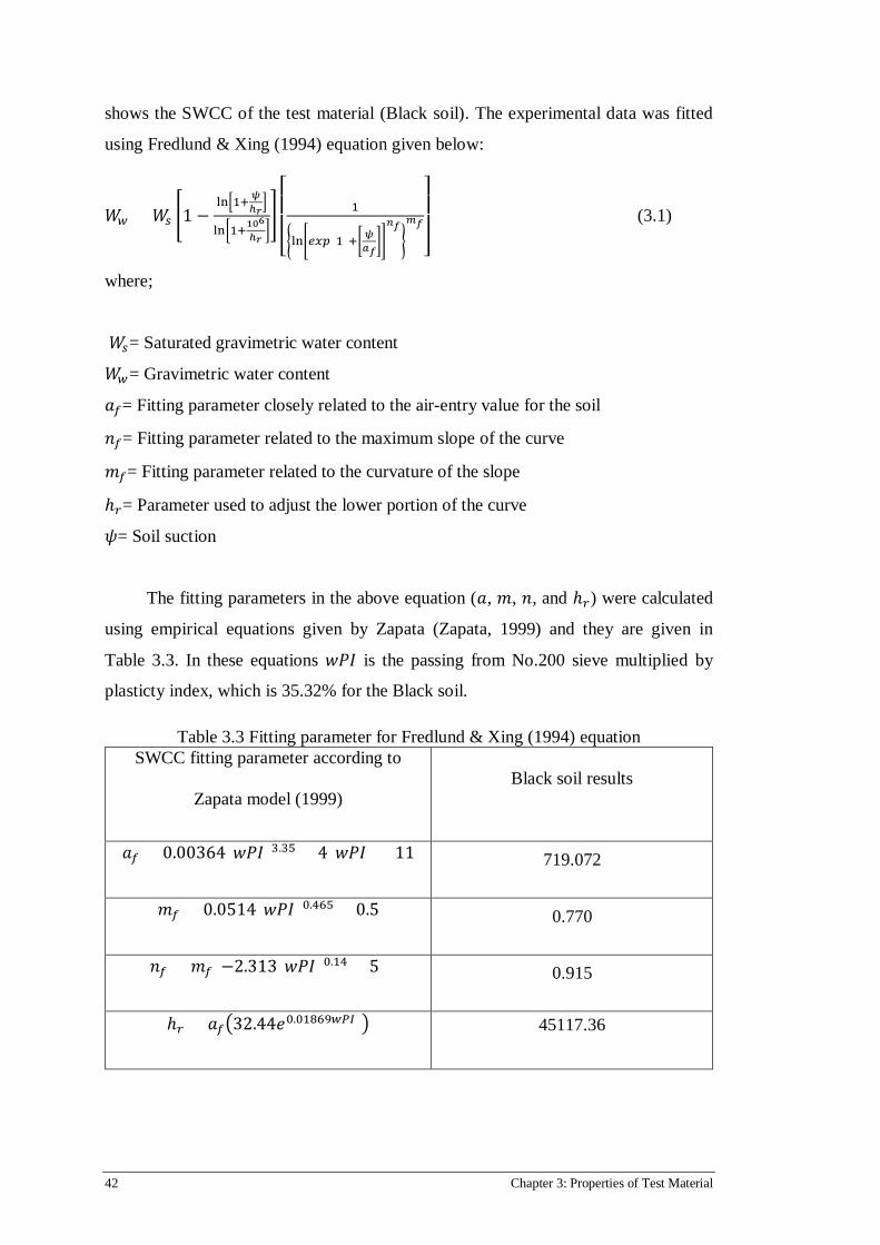
42 Chapter 3: Properties of Test Material
shows the SWCC of the test material (Black soil). The experimental data was fitted
using Fredlund & Xing (1994) equation given below:
𝑊𝑤 = 𝑊𝑠 �1 −ln�1+𝜓
ℎ𝑟�
ln�1+106
ℎ𝑟��
⎣⎢⎢⎡
1
�ln�𝑒𝑚𝑝(1)+�𝜓𝑎𝑓��𝑛𝑓�
𝑚𝑓
⎦⎥⎥⎤ (3.1)
where;
𝑊𝑠= Saturated gravimetric water content
𝑊𝑤= Gravimetric water content
𝑘𝑠= Fitting parameter closely related to the air-entry value for the soil
𝑛𝑠= Fitting parameter related to the maximum slope of the curve
𝑚𝑠= Fitting parameter related to the curvature of the slope
ℎ𝑑= Parameter used to adjust the lower portion of the curve
𝜓= Soil suction
The fitting parameters in the above equation (𝑘, 𝑚, 𝑛, and ℎ𝑑) were calculated
using empirical equations given by Zapata (Zapata, 1999) and they are given in
Table 3.3. In these equations 𝑤𝑃𝐼 is the passing from No.200 sieve multiplied by
plasticty index, which is 35.32% for the Black soil.
Table 3.3 Fitting parameter for Fredlund & Xing (1994) equation SWCC fitting parameter according to
Zapata model (1999) Black soil results
𝑘𝑠 = 0.00364(𝑤𝑃𝐼)3.35 + 4(𝑤𝑃𝐼) + 11 719.072
𝑚𝑠 = 0.0514(𝑤𝑃𝐼)0.465 + 0.5 0.770
𝑛𝑠 = 𝑚𝑠(−2.313(𝑤𝑃𝐼)0.14 + 5) 0.915
ℎ𝑑 = 𝑘𝑠�32.44𝑒0.01869𝑤𝑤𝑤)� 45117.36

Chapter 3: Properties of Test Material 43
By using calculated fitting parameters provided in Table 3.3, SWCC curve was
plotted and shown in Figure 3.11.
Figure 3.11 SWCC results and comparison with Fredlund Xing, 1994 fitting curve.
3.13 SWELLING PROPERTIES
Swelling/consolidation tests were conducted on the test material to determine
swell properties of the Black soil, such as; percentage of swelling, swelling pressure,
and hydraulic conductivity. These properties are needed to predict the heave of the
soil column test, which will be discussed in Chapters 6.
For determination of swell properties, a fully automatic electro-mechanical
oedometer Wille was used in this study. The Wille oedometer test can apply a fully
automatic range of pressure and displacement controlled with the incremental and
constant load. This oedometer apparatus uses an exchangeable load transducer and
additional sensors inputs that enable individual test conducted by defining different
measurement parameters as input control values. The software interface and
electronics control panel enable the monitoring of all the parameters during the
testing performance.
For the saturation condition, we have designed and used a separate water flow
system attached to the oedometer cell, which is not built in the machine and

44 Chapter 3: Properties of Test Material
considered as the limitation for this machine. Figure 3.12 shows the fully-automated
consolidation/swell apparatus used in this study.
Figure 3.12 Fully-controlled hydraulic apparatus for swelling and consolidation test
3.13.1 One-dimensional free swelling and swelling pressure
To conduct a one-dimensional free swell and swell pressure for the Black soil,
a soil sample was obtained from the compaction procedure. The correct amount of
soil was compacted in the compaction mould to achieve desired dry density and
gravimetric water content, which were 1.2 g/cm3 and 15%, respectively. After
extracting the compacted soil from the mould, the consolidometer ring was pushed
into the soil; then the extra parts were trimmed. 24 hours before starting the test, two
porous stones were immersed in water under vacuum to be saturated. Saturated
porous stones were then placed on the both side of the specimen and the ring with
soil sample placed in the consolidometer cell. This test was conducted according to
ASTM D4546.
An initial seating load of 7 kPa was applied to the soil specimen. Then the
consolidometer cell was filled with water. Once seating load was placed, digital

Chapter 3: Properties of Test Material 45
LVDT was started to recording the vertical displacement. After the soil specimen
stops swelling, the magnitude of swell can be measured, which was 4.30 mm for the
Black soil as shown in Figure 3.13.
Figure 3.13 Free swell test results for Black soil
Once the free swelling stabilised, a swell pressure test was performed on the
specimen to determine the swell pressure. The additional vertical loads were applied
in five steps, by applying pressures from 7 kPa to 270 kPa to consolidate the soil
specimen to its initial volume. Figure 3.14 shows the swell pressure test results.
Figure 3.14 Swell pressure test results for test material

46 Chapter 3: Properties of Test Material
According to the Figure 3.14, the swell pressure was estimated at 263 kPa for
the Black soil with 15% initial gravimetric water content, and the curve shows that
by increasing effective stress, the void ratio of soil sample reduces. Figure 3.14
illustrates the loading and unloading curves, which were used to determine swelling
pressure, 𝐶𝑃 and 𝐶𝑐.After the applied stress reaching the swelling pressure (263kPa),
the vertical load was increased to continue the consolidation process. The
compression index (𝐶𝑐), or the slope of the loading part of the curve was
determined, 0.47𝑘𝑃𝑘−1. Then the applied stress was gradually removed and the
swell index (𝐶𝑃), or the slope of rebound curve, was determined, 0.06𝑘𝑃𝑘−1.
The water content and height of the soil specimen were measured before and
after swelling test. Figure 3.15 shows the soil specimen in the consolidation ring
before and after the swell test. A large number of shrinkage cracks were observed on
the sample surface after it was oven-dried.
Figure 3.15 Soil sample tested in swell test, (a) before oven-dried, and (b) after oven-dried
3.13.2 Coefficient of permeability
The coefficient of permeability explained how easily the water can pass
through a porous material. In contrast, permeability refers specifically to the natural
properties of the soil itself rather than the effect of the type of water or fluid. To
determine the coefficient of permeability, the consolidation test was conducted.
Since the coefficient of permeability 𝑘 (𝑚/𝑃), is a function of coefficient of
consolidation 𝐶𝑣 (𝑚2 𝑃⁄ ), coefficient of volume change 𝑚𝑣(𝑚2/𝑘𝑘), and unit weight
of water 𝛾𝑤(𝑘𝑘/𝑚3); therefore, the following equation was used to determine the
coefficient of permeability;

Chapter 3: Properties of Test Material 47
𝑘 = 𝐶𝑣 × 𝑚𝑣 × 𝛾𝑤 (3. 2)
where;
𝑘= Coefficient of permeability
𝐶𝑣= Coefficient of consolidation
𝑚𝑣=Volumetric compressibility
𝛾𝑤=Unit weight of water
To obtain the coefficient of consolidation (𝐶𝐼), the soil sample was
consolidated by using oedometer from 7 kPa to 350 kPa of axial pressures. The
coefficient of consolidation was then determined from the equation below
(Casagrande's logarithm of time fitting method) by using corresponding time of 50%
consolidation (𝑡50) and the half of specimen height (𝐻𝑑𝑑) during the consolidation:
𝐶𝑉 = 0.197 �𝐻𝑑𝑟2
𝑝50� (3.4)
In this test, 𝐶𝑣 for the Black soil was calculated to be 1.87 × 10⁻⁸ 𝑚2/𝑃. To
calculate volumetric compressibility (𝑚𝑣), two different axial loads (7 and 350 kPa)
and corresponding strains, and an average values for the volume change (∆𝑉𝑉0
= 0.59)
are used over the range of total stress change ∆(𝜎𝑦 − 𝑈𝑚) as follow:
𝑚𝑣 = ∆𝑉𝑉0
∆(𝜎𝑦� − 𝑈𝑚) (3.3)
From the axial stress and volumetric strain values for the Black soil, 𝑚𝑣 was
calculated to be 3.79 × 10⁻⁴ 𝑚2/𝑘𝑁. Therefore, by using equation (3.2), the
coefficient of permeability for the test material was estimated to be 7.1 × 10⁻¹¹ 𝑚/
𝑃. Figure 3.16 shows the consolidation curve for the test material (Black soil).
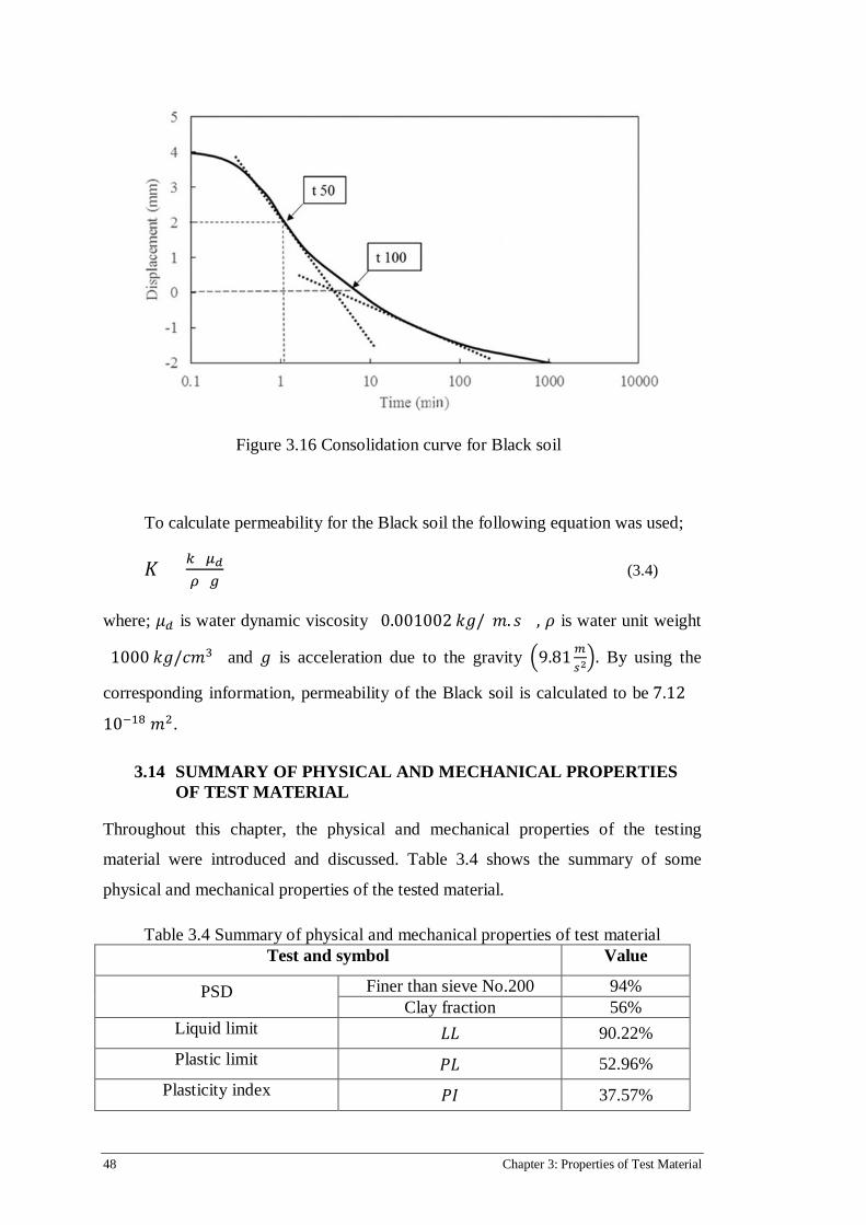
48 Chapter 3: Properties of Test Material
Figure 3.16 Consolidation curve for Black soil
To calculate permeability for the Black soil the following equation was used;
𝐾 = 𝑘×𝜇𝑑𝜌×𝑔
(3.4)
where; 𝜇𝑑 is water dynamic viscosity (0.001002 𝑘𝑘/(𝑚. 𝑃)), 𝜌 is water unit weight
(1000 𝑘𝑘/𝑐𝑚3) and 𝑘 is acceleration due to the gravity �9.81 𝑚𝑠2�. By using the
corresponding information, permeability of the Black soil is calculated to be 7.12 ×
10−18 𝑚2.
3.14 SUMMARY OF PHYSICAL AND MECHANICAL PROPERTIES OF TEST MATERIAL
Throughout this chapter, the physical and mechanical properties of the testing
material were introduced and discussed. Table 3.4 shows the summary of some
physical and mechanical properties of the tested material.
Table 3.4 Summary of physical and mechanical properties of test material Test and symbol Value
PSD Finer than sieve No.200 94% Clay fraction 56%
Liquid limit 𝐿𝐿 90.22% Plastic limit 𝑃𝐿 52.96%
Plasticity index 𝑃𝐼 37.57%
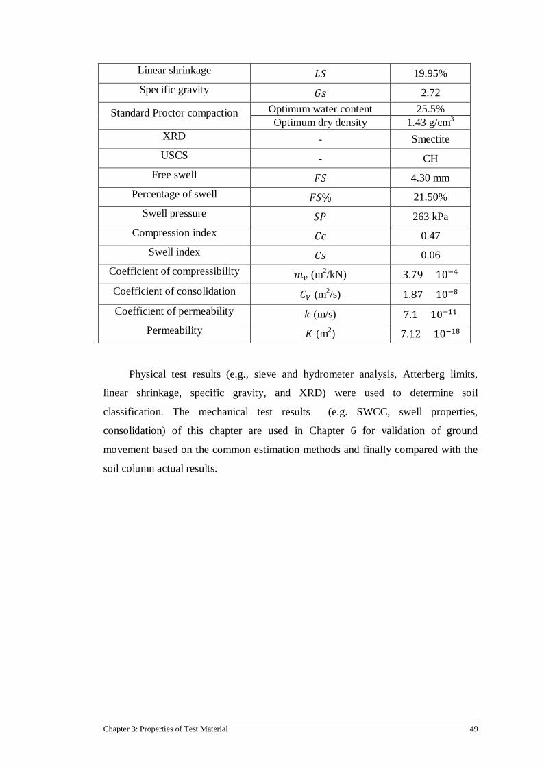
Chapter 3: Properties of Test Material 49
Linear shrinkage 𝐿𝐿 19.95% Specific gravity 𝐺𝑃 2.72
Standard Proctor compaction Optimum water content 25.5% Optimum dry density 1.43 g/cm3
XRD - Smectite USCS - CH
Free swell 𝑝𝐿 4.30 mm Percentage of swell 𝑝𝐿% 21.50%
Swell pressure 𝐿𝑃 263 kPa Compression index 𝐶𝑐 0.47
Swell index 𝐶𝑃 0.06 Coefficient of compressibility 𝑚𝑣 (m2/kN) 3.79 × 10⁻⁴ Coefficient of consolidation 𝐶𝑉 (m2/s) 1.87 × 10⁻⁸ Coefficient of permeability 𝑘 (m/s) 7.1 × 10⁻¹¹
Permeability 𝐾 (m2) 7.12 × 10⁻¹⁸
Physical test results (e.g., sieve and hydrometer analysis, Atterberg limits,
linear shrinkage, specific gravity, and XRD) were used to determine soil
classification. The mechanical test results (e.g. SWCC, swell properties,
consolidation) of this chapter are used in Chapter 6 for validation of ground
movement based on the common estimation methods and finally compared with the
soil column actual results.


Chapter 4: Soil Column and its Preparation 51
Chapter 4: Soil Column and its Preparation
4.1 INTRODUCTION
The literature review was undertaken to provide a framework based on the
available information regarding soil column studies and their limitations. This
research project was carried out by designing, constructing and testing a new
instrumented soil column with a specific configuration. This study allows control and
measurement of soil parameters through a cylindrical column under conditions that
aims to simulate the field conditions.
This experiment was designed by using a transparent acrylic cylinder with 400
mm diameter and 1200 mm height. The cylindrical column was screwed to a PVC
base plate with 480 mm diameter and 20 mm thick. 150 mm diameter porous disc is
embedded into the base plate, which has two ports for wetting and drying the soil
column from the base. The soil in the column can be instrumented to measure soil
moisture, soil suction, soil temperature, sub-soil deformation along the height of the
column.
This chapter describes the parts of soil column, sensor and their calibrations,
and the setting up of the instrumented soil column to investigate the performance of
expansive soil under wetting and drying.
4.2 DESIGN AND FABRICATION OF SOIL COLUMN
The soil column has three main parts, which are; a base, a body, and a top
arrangement. Figure 4.1 shows the parts of the soil column drawn using Solidworks
3D. The 480 mm diameter base was made of 20 mm thick PVC plate, which has a
150 mm diameter recess at the centre to place a porous disc, and two drainage ports
are connected to the recess (Figure 4.2(a)). The body of the soil column is 1200 mm
long acrylic pipe with the outer diameter of 400 mm and the wall thickness of 10
mm. Two annular rings (Figure 4.2(b) and Figure 4.3(a)) were glued to the top and
bottom end of the cylinder. The bottom end of the acrylic pipe was glued to an
annular ring (Figure 4.2(b)), which was then bolted to the base plate. An O-ring was
placed between the annular ring and the base plate to prevent water leakage during
the test.

52 Chapter 4: Soil Column and its Preparation
Figure 4.1 Parts of soil column; (a) PVC base, (b) bottom annular ring, (c) tensiometer mounting block, (d) top annular ring, and (e) LVDT mounting plate
Figure 4.2 (a) Base plate, and (b) bottom annular ring

Chapter 4: Soil Column and its Preparation 53
18 mm diameter holes were drilled through the cylindrical wall to install the
sensors. Holes were made at five different levels along the height of the column. At
each level, four holes were drilled with 90° spacing.
The LVDT mounting plate, shown in Figure 4.3(b), is mounted at the top of the
column by bolting to the top annular ring. The LVDTs are mounted on the plate as
shown in Figure 4.1. The LVDT needle is screwed to the vertical shaft of the
settlement plate (Figure 4.3(c)). The vertical shaft of the settlement plate moves
through the guiding block (Figure 4.3(d)), which is attached to the LVDT mounting
plate below the LVDT. These guiding blocks are made of acrylic.
Figure 4.3 (a) Top annular ring, (b) LVDT mounting plate, (c) settlement plate, and (d) guiding block
The settlement plate as shown in Figure 4.3(c) was designed and fabricated to
measure soil displacement in the different depths in the soil column. The settlement
plate consists of a 100 mm diameter acrylic disc (10 mm thick) and a 10 mm
diameter acrylic rod, which is glued to the disc. The LVDT needle can be screwed to
the top of the rod. The rod moves in a sleeve in soil to minimise soil frictional effect
on the rod movement. Five settlement plates were made with different rod lengths so

54 Chapter 4: Soil Column and its Preparation
that they can be used to measure the sub-soil deformation at different depths in the
column.
4.3 SENSORS USED IN SOIL COLUMN AND CALIBRATIONS
The soil column in this study was designed and instrumented to measure soil
volumetric water content, suction, temperature, and sub-soil deformation at five
different depths. This soil column was instrumented with five volumetric water
content sensors, six thermocouples, six tensiometers, five sub-soil displacement
devices and one relative humidity sensor. This section briefly describes each sensor
type and its calibration.
4.3.1 Water content sensors and calibrations
EC-5 (Figure 4.4) moisture sensor was used to measure the volumetric water
content in the soil column. The voltage output of the sensor is linearly proportional to
the dielectric properties of the soil, which depend on soil moisture content. The
specifications of EC-5 are given in Table 4.1 (Decagon Devices, Inc.).
Figure 4.4 Water content sensor EC-5 used in soil column Table 4.1 Water content sensor specification
Specification Measuring ranges
Accuracy ±1-2% with soil specific calibration
Resolutıon 0.1% (mineral soil)
Range Between 0 and 100%
Dimensıons 8.9 ×1.8 × 0.7 cm
Measurement time 10 ms
Output Voltage
Temperature -40°C to +50°C

Chapter 4: Soil Column and its Preparation 55
All 5 EC-5 moisture sensors were calibrated with the test material (Black Soil)
to achieve the high accuracy in measuring water content in the soil column. To
perform the sensor calibration, oven dried soil was mixed with water to achieve a
gravimetric water content of 15%, 30%, 40%, and 50%. As shown in Figure 4.5(a
and b), each moist soil sample was then compacted into a PVC ring to achieve the
dry density of 1.2 g/cm3 . All five EC-5 sensors were then inserted into the soil and
voltage outputs of sensors were recorded for 2 hours by minimising the moisture
variation in the sample by wrapping in cling wrap as shown in Figure 4.5(c). Once
the sensors outputs were stabilised, the sample’s volumetric water content was
plotted with voltage outputs of the sensors.
Figure 4.5 Calibration of water content sensors; (a and b) sample compaction, and (c) inserting sensors into soil and cover with plastic wrap
As shown in Figure 4.6, a linear relationship between the volumetric water
content and voltage sensor output was developed, and it is given in Equation 4.1.
Figure 4.6 Calibration results for water content sensors

56 Chapter 4: Soil Column and its Preparation
𝑌 = 138.29𝑋 − 93.913 (4.1)
where; 𝑌 is volumetric water content value (%) and X is sensors output in Volts.
4.3.2 Displacement sensors and calibrations
Five LVDTs were used to measure sub-soil displacements. The measurement
range of LVDTs is up to ±110 mm. Figure 4.7 shows an LVDT, which used in this
research. The specifications of LVDT are given in Table 4.2 (Miran technology).
Figure 4.7 LVDT used for measuring sub-soil displacement in soil column
Table 4.2 Specifications of LVDT Specification Measuring ranges
Accuracy ± 0.05%
Range Between 1 and 110 mm
Measurement time 10 ms
Output Voltage
A customised data logger was developed to measure the output of LVDT in
Volts as the needle of the LVDT moves. Each LVDT was then calibrated by
measuring output voltage as its needle was moved for known distances as shown in
Figure 4.8.

Chapter 4: Soil Column and its Preparation 57
Figure 4.8 Calibration process for LVDT
Figure 4.9 Calibration results for LVDTs
Figure 4.9 shows the LVDT needle displacement and its corresponding output
voltage for all five LVDTs. The data was fitted to a straight line, which is given by
the following Equation:
𝑌 = −23.236𝑋 + 120.8 (4.2)
where; 𝑌 is the displacement (mm) and 𝑋 is the output readings of LVDTs in Volts.
4.3.3 Suction sensors and calibrations
To measure the matric suction in the soil column, two types of sensors were
used. They are three MPS-6s (use indirect method) and three tensiometers (direct
method). Figure 4.10 shows an MPS-6 used in this study.

58 Chapter 4: Soil Column and its Preparation
Figure 4.10 MPS-6 suction sensor
The MPS-6 sensor consists of water content sensors surrounded by two porous
ceramic discs. When the sensor with saturated ceramic discs is installed in soil, water
in the ceramic disc equilibrates with the soil moisture achieving the matric suction in
the ceramic disc, which is the same as the soil’s matric suction. At this stage, the
water content in the ceramic disc is measured by the water content sensors, and it is
converted to matric suction by using the soil water characteristic curve (SWCC) of
the ceramic disc. The three MPS-6 sensors used in this study were factory calibrated
with six-point calibration with its dedicated logging system (EM50) to give the soil
matric suction in kPa. The specifications of the MPS-6 sensor is given in Table 4.3
(Decagon Devices, Inc.).
Table 4.3 Specifications of MPS-6 sensor Specification Measuring ranges
Accuracy ±(10% + 2 kPa) from -9 to -100 kPa
Soil Temperature: ± 1°C
Resolution Soil Water Potential: 0.1 kPa
Soil Temperature: 0.1°C
Range soil water potential -9 to -100,000 kPa
Soil temperature -40° to 60°C
Equilibration time 10 min to 1 hr depending on soil water
potential
Sensor dimensions 9.6 cm (l) x 3.5 cm (w) x 1.5 cm (d)

Chapter 4: Soil Column and its Preparation 59
Since MPS-6 has the low accuracy (10% of reading + 2 kPa) for the low
suction range (9 kPa to 100 kPa), three tensiometers designed and manufactured at
QUT were used in the soil column to measure the low suction more accurately.
Figure 4.11 Shows the laboratory designed and manufactured tensiometer. The
tensiometer consists of a pressure transducer, ceramic tip, and an acrylic block. Three
of these tensiometers were used in the soil column study.
Figure 4.11 Tensiometer which developed at QUT
A pressure transducer, which can measure negative pressure up to -100 kPa is
directly connected to the acrylic block. The ceramic cup is connected to the acrylic
block using two thin tubes so that flushing can be done to remove the cavitated air
bubbles. The ceramic tip with 100 kPa air entry value (AEV) was saturated under
vacuum to obtain maximum measured suction. Figure 4.12 shows the schematic
diagram of the tensiometer.

60 Chapter 4: Soil Column and its Preparation
Figure 4.12 Schematic diagram of laboratory designed tensiometer
Figure 4.12 shows during setting up the soil column, an acrylic block of the
tensiometers were bolted on the wall of the soil column, and ceramic tips were
embedded in the soil. Later these two parts were connected by two thin tubes. Then
water was injected through the inlet tube to the ceramic tip. In the ceramic tip water
circulated and flushed out through the outlet tube. This process was repeated a
couple of times to push out air bubbles, which were trapped in the ceramic tip and,
ceramic tip became saturated. Two valves controlled the water flow in and out of the
acrylic block and provided a sealed condition for suction measurement.
When the soils around the ceramic tip were dried out, they sucked the water
from sensor’s water reservoir and applied negative pressure to the pressure
transducer. Conversely, when the soils around ceramic tip become wet, water is
pushed into the water reservoir, and positive pressure is applied to the pressure
transducer.

Chapter 4: Soil Column and its Preparation 61
The pressure transducers were calibrated to measure negative pressure by
connecting the transducer to a connecting block, which was connected to a vacuum
pump to apply controlled negative pressure (Figure 4.13).
Figure 4.13 A pressure transducer is connected to block to calibrate for negative pressure
The pressure transducers were calibrated in the negative pressures range, and
the calibration curve was plotted. Calibration results are shown in Figure 4.14.
Figure 4.14 Pressure transducers calibration curve

62 Chapter 4: Soil Column and its Preparation
Figure 4.14 shows the sensor output voltage values for the applied negative
pressure values. The calibration data of all three transducers were fitted to a linear
trend line, which is represented by Equation 4.3.
𝑌 = 647.17𝑋 + 4.4737 (4.3)
where; 𝑌 is pressure in kPa and 𝑋 is voltage output of transducers Volts.
4.3.4 Thermocouples and calibrations
Six thermocouples were utilised in the soil column for measuring sub-soil’s
temperature. The customised logger was able to record the responses of
thermocouples in Volts. Therefore, it was required to calibrate all six thermocouples.
As shown in Figure 4.15, all six thermocouples were placed in water at
different temperatures. The temperature of the water was measured using a
thermometer, and the thermocouple output voltages were recorded. The actual
temperature of water and the corresponding voltage outputs of thermocouples were
plotted as shown in Figure 4.16.
Figure 4.15 Thermocouples calibration process by submerging in water with different temperatures

Chapter 4: Soil Column and its Preparation 63
Figure 4.16 Thermocouples calibration results
The calibration data are shown in Figure 4.16 were fitted to a linear trendline,
which is represented by Equation 4.4 and can be used to convert the voltage outputs
of thermocouples to degrees Celsius.
𝑌 = 91.72𝑋 + 1.2781 (4.4)
where; 𝑌 is the temperature in degrees of Celsius and 𝑋 is the thermocouple’s output
voltage in Volts.
4.3.5 Relative humidity
Figure 4.17 shows the unit used to measure the relative humidity and
temperature of surrounding air around of the column during wetting and drying. The
unit can be connected to a computer to record the data at the specified time interval.
Table 4.4 shows the specifications of relative humidity sensor used in this study (RS
Components Pte Ltd).

64 Chapter 4: Soil Column and its Preparation
Figure 4.17 Relative humidity sensor with a calibrated built-in system
Table 4.4 Specifications of relative humidity sensor Feature item Practical ranges
Humidity range 20 → 90 %
Temperature range -50 → +70 °C
Humidity accuracy ±5% (25 → 80%) ±10% elsewhere %
Temperature
accuracy ±1°C (0 → 40 °C) ±2 °C
Resolution 0.5°C/RH %
Dimensions 10.8 x 5.8 x 1.5 cm
4.4 SETTING UP OF SOIL COLUMN
Natural Black soil was collected (test pits) from Ipswich, Queensland (Figure
4.18(a)) and crushed to smaller lumps (Figure 4.18(b)). After oven drying, 15% of
water was added and mixed using a mixture as shown in Figure 4.18(c). The soil was
then left overnight in a closed container for moisture homogenisation (Figure
4.18(d)).

Chapter 4: Soil Column and its Preparation 65
Figure 4.18 Soil sample preparation process
As shown in Figure 4.19 (a) and (b), a sand layer was first placed at the bottom
of the soil column and compacted to achieve the thickness of 25 mm. A geotextile
was then placed on the top of the sand layer (Figure 4.19 (c)). It is expected sand,
and geotextile will allow adequate drainage at the base of the soil column and
minimise the contamination of sand with Black soil.

66 Chapter 4: Soil Column and its Preparation
Figure 4.19 Process of filling soil column; (a) placing sand, (b) compaction of sand in column, and (c) placing a geotextile layer
The following steps were followed to fill the soil column and to install the sensors:
1. 8.24 kg of wet soil ( with 15% gravimetric water content) was poured into
the column and compacted to achieve the layer thickness of 50 mm. Since the
inner diameter of the column is 390 mm, the dry density of the layer was 1.2
g/cm3 (Figure 4.20 (a)).
2. Step 1 was repeated four times to achieve the soil height of 200 mm, and then
the first set of sensors (WC1, LVDT 1, TEM1, and LS1) were placed as
shown in Figure 4.20 (b).

Chapter 4: Soil Column and its Preparation 67
3. Step 1 was repeated for another six times to achieve the height of Black soil
height of 500 mm and then the second set of sensorsWC3, LVDT2, TEM3
and HS1 (Figure 4.20(c)) were placed.
4. 1000 mm height of Black soil column was achieved by repeating step 1 for
20 times. The sensors were installed at specified levels as the filling of the
column was progressed.
Figure 4.20 Soil column filling process; (a) first layer filling, (b) placing of first series of sensors, (c) placing of second series of sensors, and (d) placing of third
series of sensors
All tensiometers were kept in the distilled water under a vacuum condition to
be fully saturated 24 hours before setting up in the soil column.
All the LVDTs were screwed to a steel part (Figure 4.21 (a) and (b)), and
LVDT cores were attached to an acrylic bar and a plate (Figure 4.21 (c)) to measure
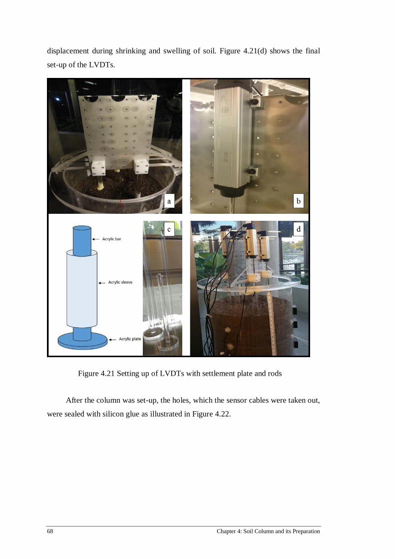
68 Chapter 4: Soil Column and its Preparation
displacement during shrinking and swelling of soil. Figure 4.21(d) shows the final
set-up of the LVDTs.
Figure 4.21 Setting up of LVDTs with settlement plate and rods
After the column was set-up, the holes, which the sensor cables were taken out,
were sealed with silicon glue as illustrated in Figure 4.22.

Chapter 4: Soil Column and its Preparation 69
Figure 4.22 (a) Before sealing holes, and (b) after sealing holes with silicon glue
Table 4.5 summarised the soil column sensors, from the top to the bottom of
the column.
Table 4.5 Sensor types and their location in soil column Depth from
the top surface (mm)
Sensors position
Water content Thermocouple LVDT
MPS-6 (High
suction)
Tensiometers (Low
suction)
Surface - TEM6 - - -
30 - - LVDT5 - -
50 WC5 TEM5 LVDT4 S-High3 -
150 WC4 TEM4 LVDT3 S-High2 S-Low3
300 WC3 TEM3 LVDT2 S-High1 -
500 WC2 TEM2 - - S-Low2
800 WC1 TEM1 LVDT1 - S-Low1

70 Chapter 4: Soil Column and its Preparation
The schematic design of the final set-up of the soil column is presented in
Figure 4.23.
Figure 4.23 Schematic design of final set-up
The whole soil column set-up took more than 12 hours, including all sensors
being connected to the data loggers and a computer.
4.5 DRYING AND WETTING OF SOIL COLUMN
A complete cycle of wetting-drying was performed with the soil column. The
employed methodology is provided in the following sections.
4.5.1 Wetting cycle
The constant head wetting from the top of the column was provided by
employing a Marriot bottle. Figure 4.24 shows the Marriot bottle, which was used in
this study.

Chapter 4: Soil Column and its Preparation 71
Figure 4.24 Marriot bottle
The Mariotte bottle is a device that can provide constant water flow by keeping
the pressure of the air inlet at the same pressure as the outlet of the tank. The
Mariotte bottle was designed as a closed system except an inlet pipe at the top of the
water tank and outlet valve at the bottom. The inserted vertical pipe can control the
exit water pressure. As soon as the water begins flowing out to the soil column from
the outlet valve, the pressure inside the vertical pipe decreased below atmospheric
pressure. This decreasing pressure pushes air to the vertical pipe, keeping the
pressure at the bottom of the pipe at atmospheric pressure. By changing the water
level in the soil column, the pressure at the exit valve will remain constant at an
atmospheric level.
The Marriot bottle was maintained at a constant water head of 4cm during the
wetting process on top of the soil column. The wetting process of the soil column
took nearly four months (Figure 4.25).

72 Chapter 4: Soil Column and its Preparation
Figure 4.25 Wetting cycle by using a constant water flow condition
4.5.2 Drying cycle
Drying cycle was performed by employing a heating lamp with 115 VAC,
50/60 Hz power usage. The heating lamp was mounted on an adjustable stand
support with extension arms helped to adjust the exposing direction to the soil
column. Since the heating lamp can produce excessive temperature against the
acrylic column, a trial test was carried out to determine the optimum lamp distance
from the soil column. The optimum distance was determined 30cm from the soil
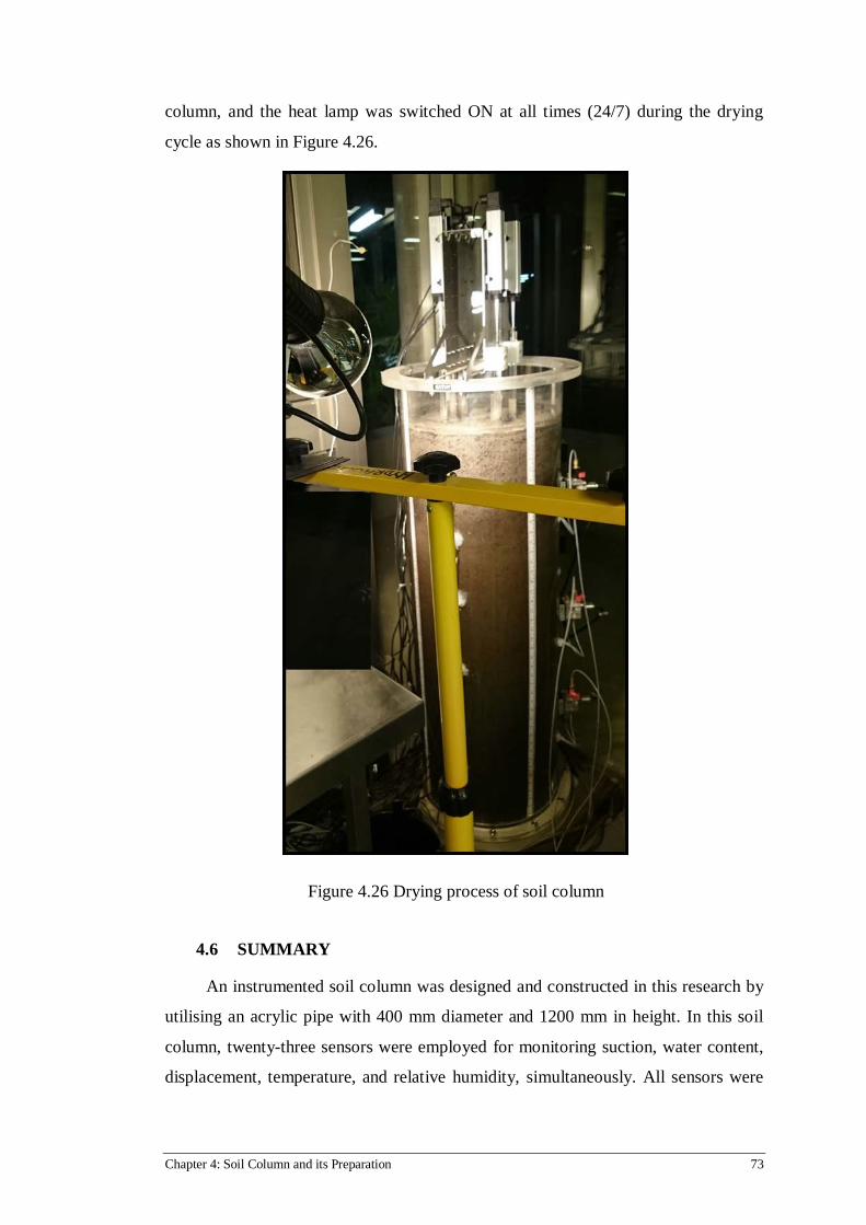
Chapter 4: Soil Column and its Preparation 73
column, and the heat lamp was switched ON at all times (24/7) during the drying
cycle as shown in Figure 4.26.
Figure 4.26 Drying process of soil column
4.6 SUMMARY
An instrumented soil column was designed and constructed in this research by
utilising an acrylic pipe with 400 mm diameter and 1200 mm in height. In this soil
column, twenty-three sensors were employed for monitoring suction, water content,
displacement, temperature, and relative humidity, simultaneously. All sensors were

74 Chapter 4: Soil Column and its Preparation
calibrated and used for continuous measuring of soil response during the wetting and
drying cycles.
According to the literature, previous soil column studies have been conducted
on smaller dimensions soil columns; however, in this research, a new soil column
was designed with the larger dimensions to reduce any boundary condition effects.
The results of this soil column test will be discussed in the next chapter and
validation of some heave prediction methods using the results of the wetting cycle of
the soil column are described in Chapter 6.

Chapter 5: Results and Discussion 75
Chapter 5: Results and Discussion
5.1 INTRODUCTION
As described in Chapter 4, the instrumented soil column was prepared using a
natural expansive soil (Black Soil) collected from Ipswich area in Queensland,
Australia. The soil with initial moisture content (gravimetric) of 15% was compacted
into the column to achieve 1.2 g/cm3 dry density. After connecting all 23 sensors
(including humidity meter) to the data logging system, the soil column was left for
two days to stabilise sensor readings. The soil column was then subjected to wetting
from the top for four months (August – December 2015). The laboratory developed
Marriott bottle was employed to supply water to the top surface of the column. The
Marriott bottle maintained a 40 mm head of ponding water at the surface of the soil
column allowing water to infiltrate into the soil. Once the wetting of soil column was
completed, a heating lamp was employed to simulate drying condition in the soil
column from December 2015 to March 2016.
During the period of soil column test (eight months), the following parameters were
recorded at the depth of soil column:
• Soil moisture content
• Soil suction
• Sub-soil deformation
• Soil temperature
Air temperature and relative humidity above the top surface of the soil column were
also recorded.
This chapter presents and discusses the recorded data during the entire period
of the soil column test.
5.2 SOIL MOISTURE CONTENT
Five soil moisture sensors (WC5, WC4, WC3, WC2, and WC1), which were
calibrated with the test material and corrected for temperature were installed at five
different depths in the soil column (50 mm, 150 mm, 300 mm, 500 mm, and 800
mm). Figure 5.1 shows responses of the water content sensors during wetting
(August – December 2015) and drying (December 2015 – April 2016).

76 Chapter 5: Results and Discussion
Figure 5.1 Soil water content monitoring during wetting-drying cycle
As shown in Figure 5.1, water content for all depths started from 18% as the
initial water content value and increased during the wetting months. WC5 and WC4
that were embedded in the depth of 50 mm and 150 mm were quickly wetted and
experienced a quick jump to about 59% and remained at the same amount until the
end of the wetting cycle. WC3 was wetted during the second month and reached to
57% at the maximum level. Later, in the third and fourth months, WC2 and WC1
became wetted (reached to 57%) at the depths 500 mm and 800 mm, accordingly.
At the second month of the drying cycle, water content quickly decreased at the
depth of 50 mm and 150 mm, respectively. There were few fluctuations monitored
for the deepest water content sensors, and they remained wet after four months.
However, the mid layer of the soil column showed a small reduction in the moisture
content, to 45%. Figure 5.2 shows the water content changes over the depth that was
monitored in the wetting cycle.

Chapter 5: Results and Discussion 77
Figure 5.2 Soil water content variation during wetting cycle along depth of soil
column
As shown in Figure 5.2, after one month (in September 2015), WC5 (at the
depth of 50 mm) and WC4 (at the depth of 150 mm) reached the full saturation
(volumetric water content about 60%) condition, then they stabilised and stayed
constant until the end of November 2015. However, in the depth below 300 mm, it
took a long time to reach the saturated condition and water content gradually
increased with the depth. As a result, soil at the depth of 800 mm in the soil column
(WC1) reached saturation after four months.
The drying of the soil column started in December 2015 by setting up a heat
lamp.As shown in Figure 5.1 and 5.3, the soil water content decreased from the
surface to the bottom of the soil column. There was a significant difference between
the water content of top (15.03%) and bottom (56.60%) layers at the end of March
2016 (end of drying cycle). Figure 5.3 shows the water content along the depth of the
column at the end of November (just after wetting), December, January, February,
and March during the drying process of the soil column. It revealed that four months
of drying has not caused a change in the water content below the 500 mm depth of
the column.

78 Chapter 5: Results and Discussion
Figure 5.3 Soil water content profile variation with time during drying cycle
Figure 5.4 illustrates the water content profile (water content with the depth of
the column) variation with time during the wetting-drying cycle. As expected, after
the wet soil was compacted into the column, the initial volumetric water content was
about 18% along the depth of the column. Once the column was fully wetted,
volumetric water content along the depth was in the range of 59%-57% (November).
It can be assumed the column to be fully saturated at the end of November. However,
the volumetric water content along the depth is not uniform; higher water content at
the top compared to the bottom. The reason for this variation could be the decrease in
density of soil in the top of the soil column compared to the bottom due to soil
swelling. The lower the density, the higher the saturated volumetric water content.
The water content profile in each month (August to November) clearly indicates the
gradual wetting of the soil column from the top.
The water content profiles of the column from November to March clearly
demonstrate the drying of the soil column from the top. In four months, the soil water
content down to 500 mm was affected by the environment. The soil column has
clearly simulated the reactive depth of the column (the soil depth affected by the
environment), which is similar to the in-situ conditions.

Chapter 5: Results and Discussion 79
Figure 5.4 Soil water content variation with time during wetting-drying cycles
5.3 SOIL SUCTION
To measure the soil suction along the depth of the soil column, three MPS-6
sensors (high suction measurement) and three tensiometers (low suction
measurement) were used. MPS-6 sensors were installed at 50 mm, 150 mm, and 300
mm depths. Tensiometers were installed at 150 mm, 500 mm, and 800 mm depths.
The initial suction profile shown in Figure 5.5 is based on the reading of MPS-6
sensors only. Initially, the suction along the column was uniform, and it was around
3000 kPa. As the wetting progresses, the suction decreases following the profiles
shown in Figure 5.5. At the end of the wetting (November), the suction ranged from
6 kPa–10 kPa along the column. The suction profiles are given in Figure 5.5 clearly
demonstrate the wetting process (August to November), and they are consistent with
the measured water content profiles. Once the soil column was fully wetted (end of
November), tensiometers were activated.

80 Chapter 5: Results and Discussion
Figure 5.5 Soil suction profile during wetting cycle
Figure 5.6 illustrates suction change during the drying cycle over the time and
depth in the soil column. Since the soil was in the fully saturated condition in
November 2015 (Figure 5.2), suction was less than 10 kPa along the depth of the
column at the end of the wetting cycle. As the soil dries from the top, there was a
significant change in the suction down to the depth of 500 mm. After four months of
drying, the suction near the surface reached about 3200 kPa. However, no significant
suction change was observed below the depth of 500 mm compared with above the
depth of 500 mm. These suction profiles were obtained during drying are consistent
with the observed water content profiles.
Figure 5.6 Soil suction profile during drying phase of soil column

Chapter 5: Results and Discussion 81
Figure 5.7 depicts the suction variation with the depth and the time during both
the wetting and drying cycles.
Figure 5.7 Soil suction profile during wetting-drying cycle of soil column
As Figure 5.7 shows, measuring the suction is distinguished in three main
zones as:
1. The surface zone that is reaching a depth of about 150 mm in the soil column and
such that the pore water pressure is very sensitive to a water content change, and it is
increasing quickly with the decreasing of water content amount.
2. The shallow zone that is ranged from the depth of about 150-500 mm in the soil
column, where the pore water pressure is very slowly increasing with depth.
3. The deep zone is extended to the depth under 500 mm, where the pore water
pressure practically does not change and remained constant.
5.4 SUB-SOIL DISPLACEMENT
The sub-soil displacements were measured by LVDTs, which were attached to
the custom designed settlement plates and were discussed in Chapter 4. LVDT5.
LVDT4, LVDT3, LVDT2, and LVDT1 were set to measure the sub-soil deformation
at the depth of 30 mm, 50 mm, 150 mm, 300 mm, and 800 mm. Figure 5.8 depicts
the sub-soil displacement over the time during wetting and drying of the soil column.
As shown in Figure 5.8, a 56.7 mm soil heave was observed at the surface of
the soil column (30 mm depth) at the end of wetting. The soil did not heave at the

82 Chapter 5: Results and Discussion
depth of 800 mm, in fact, it consolidated (downward movement) about 2.5 mm. As
shown in Figure 5.8, the soil swelling decreases with the depth of soil column, and it
can be caused by the increase in overburden pressure with the depth.
Figure 5.8 Sub-soil displacement monitoring during wetting- drying cycle
As shown in Figure 5.9, at the end of four months of drying, the surface of the
soil column shrunk by about 10 mm (at 30 mm and 50 mm depths). No soil shrinking
was observed at depth 500 mm and below. This is consistent with the measured
water content, and suction during drying as no significant change in water content or
suction was observed at 300 mm depth and below.
Figure 5.9 Sub-soil displacement profile after wetting and drying of soil column

Chapter 5: Results and Discussion 83
5.5 SOIL TEMPERATURE AND SURROUNDING ENVIRONMENTAL CONDITIONS
Six thermocouples (TEM6, TEM5, TEM4, TEM3, TEM2, and TEM1) were
installed at six different depths in the soil column (surface, 50 mm, 150 mm, 300
mm, 500 mm, and 800 mm). Figure 5.10 shows responses of these thermocouples
during wetting (August – December 2015) and drying (December 2015 – April
2016).
Figure 5.10 Temperature variation during wetting-drying over depth of soil column
As shown in Figure 5.10, the temperature for all depths started from 21-22°C
(August 2015) and reached 24°C at the end of wetting months (December 2015).
There were a few fluctuations were monitored due to the room temperature change
during August – December 2015.
The drying of the soil column started in December 2015 by setting up a heat
lamp. As shown in Figure 5.10, TEM6 and TEM5 that were embedded in the surface
and 50 mm experienced a quick jump to about 35°C and were gradually reached and
stayed constant at 37°C during drying cycle (December 2015–April 2016). The
temperature in the mid layer of the soil column (TEM 3) gradually increased up to
approximately 31°C. However, below the 500 mm depth (TEM1, TEM2, and TEM4)
of the column temperature didn’t change and remained constant (about 25°C).

84 Chapter 5: Results and Discussion
Figure 5.11 Relative humidity variation during wetting-drying cycle
As shown in Figure 5.11, the relative humidity (RH) increases during the
wetting cycles (up to 80%) while it varies between 55% and 65% for drying months.
Since wetting cycle experienced lower temperature than drying cycle, the relative
humidity showed higher values between August and December 2015.
5.6 SUMMARY
Wetting and drying cycles were performed on expansive soil by using the
instrumented soil column. From the installation of the probes in August 2015 to
March 2016, there was no significant issue with sensors, and all the sensors showed a
change in data and measurements were recorded at one-minute intervals by a data
logger.
The moisture content of the soil was recorded during the wetting and drying
cycles by using five water content probes. The wetting cycle was performed, and
results showed that initial water content along the soil column was around 18%. At
the start of the wetting cycle, WC4 (at depth 150 mm) and WC5 (at depth 50 mm)
jumped quickly to almost 59% and remained constant during wetting. After one
month (September 2015), WC3 (at depth 300 mm) gradually increased to about 57%
and stabilised. After two months (October 2015), WC2 (at depth 500 mm) and WC1
(at depth 800 mm) reached 55% and remained constant. Drying cycle was performed
by using a heat lamp on top of the soil column, and the results showed that WC5 (at
depth 50 mm) and WC4 (at depth 150 mm) dropped to 15% and the end of drying

Chapter 5: Results and Discussion 85
(April 2016). WC3 (at depth 300 mm) gradually decreased to about 45%, while WC1
(at depth 800 mm) and WC2 (at depth 500 mm) remained almost constant.
Three MP6 probes (high suction measurement) and three tensiometers (low
suction measurement) were placed at 50 mm, 150 mm, 300 mm, 500 mm, and 800
mm depths in the soil column. The suction measurement initially was uniformed
about 3000 kPa but by starting wetting cycle, suction decreased up to 6-10 kPa along
the column at December 2015. In drying cycle, suction increased by decreasing the
water content in the soil column and reached to 3200kPa at the end of March 2016.
To measure sub-soil displacements during the wetting and drying cycles, five
LVDT were placed at 30 mm, 50 mm, 150 mm, 300 mm, and 800 mm depths in the
soil column. Displacement results indicated that during wetting, the maximum
vertical movement of tested material was recorded 56.7 mm at the surface in fact soil
in the bottom layer consolidated about 2.5 mm as a result of overburden pressure. In
drying cycle, soil surface shrunk 10 mm, but there was no shrinking observed below
300 mm.
Six thermocouples were placed in different depths and measured the soil
temperature during the test. During the wetting, temperature for all depths fluctuated
between 21ºC and 24ºC. However, during drying temperature jumped to 37ºC at the
surface and gradually increased up to 31ºC at 150 mm depth. A small increase was
recorded for the depth below 300 mm, which then fluctuated between 25ºC and 27ºC.
A relative humidity probe was used to monitor the humidity of the surrounded
environment of the soil column during the wetting and drying cycles. Results showed
that humidity level was increased up to 80% in the wetting time, while it was
recorded between 55% and 65% for drying period.
These results will be used for validation of some commonly used heave
prediction methods in Chapter 6.

86 Chapter 5: Results and Discussion

Chapter 6: Heave Prediction 87
Chapter 6: Heave Prediction
6.1 INTRODUCTION
It is important to estimate/predict the free ground movement in soil caused by
climatic variations in designing lightweight structures, such as residential house
footings, pavements, and shallow depth pipes, to be constructed on/in expansive
soils. There are some prediction methods available in the literature. These methods
require swelling properties, index properties, and water content and suction profiles
along the reactive depth. These parameters vary depending on soil type and climatic
zone. Most of these heave/characteristic surface movement estimation/prediction
methods have been validated only for particular soils and the particular climatic
conditions. Further, it is very difficult to validate heave estimation methods for the
natural ground due to the uncontrolled condition of climatic parameters and soil
properties. The first step, for heave prediction/estimation methods should be
validated in laboratory soil column tests, which can be conducted under controlled
conditions. The boundary effects due to small column diameter and lack of soil
column tests on expansive soil in the literature were the issues when validating these
methods. The instrumented soil column in this study has sufficiently addressed these
issues. Therefore, the results of soil column test in this study are used to attempt to
validate three heave estimation methods.
Three ground heave prediction methods that were chosen in this study are:
• Prediction method 1 (Aitchison (1973))
• Prediction method 3 (Fredlund (1983))
• Prediction method 2 (Fityus and Smith (1998))
These methods are widely used by geotechnical engineers to predict the ground
movement. Each method including required parameters will first be described in the
following sections. Then, each method is used to estimate the heave of the surface of
the soil column during wetting using laboratory-measured soil properties and
monitored water content and suction profiles. The estimated values are then
compared with measured surface heave of the soil column (56.7 mm). The evaluation
of these methods will provide insights into the method’s accuracy, reliability, and

88 Chapter 6: Heave Prediction
consistency. If they are proven adequate, they need to be further validated using field
monitoring data before introducing them into engineering practice.
6.2 PREDICTION METHOD 1
In this section, the Aitchison (1973) heave estimation method is briefly
described and then applied to estimate the surface heave in the soil column during
wetting and finally the results are compared with the measured surface heave in the
soil column.
This method is used in the residential slabs and footings design code in
Australia (AS2870) for estimating the ground movement on expansive soils. The
method is represented by equation (6.1):
ΔH = 1100 ∫ IPtΔu ΔhHs
0 (6.1)
where;
𝛥𝐻= The heave of the soil layer under investigation
𝐻𝑃= Reactive depth of the ground (the depth, which is affected by the climatic
conditions)
𝐼𝑤𝑝= The soil instability index
𝛥𝑢= Change in Suction in (pF)
𝛥ℎ= Soil layer thickness
Equation (6.1) is used to calculate the maximum soil heave in the column by
considering the initial state (after filling the soil column) and full saturation of the
column. At the initial state, the matric suction along the depth of the column was
uniform, and it was approximately 3200 kPa. When the column was fully saturated,
the matric suction was approximately 20 kPa. In both initial and saturated conditions,
the suction was uniform along the depth of the soil column and therefore it is not
necessary to divide the soil column into sub-layers. When applying Equation (6.1),
the height of the soil column (100 cm) was considered as one layer and the equation
is used to calculate the soil heave. Therefore:
𝐻𝑃 = 𝛥ℎ = 100 𝑐𝑚
𝛥𝑢 = 𝑙𝑜𝑘10 (3200/9.8 × 100) − 𝑙𝑜𝑘10 (20/9.8 × 100) = 𝑙𝑜𝑘10 (3200/20) = 2.20

Chapter 6: Heave Prediction 89
Instability index, 𝐼𝑤𝑝 is given by the equation (6.2).
𝐼𝑝𝑝 =∆𝐿
𝐿�∆𝑤
∙ ∆𝑤∆𝑈
(6.2)
The ratio (∆𝐿
𝐿�∆𝑤
), can be obtained from free swelling test. In the free swelling
test discussed in Chapter 3, the sample was prepared with initial moisture content of
15% and it was saturated allowing the sample to free swell. After the swelling was
completed, swelling strain (20%) and the final water content (50%) were calculated
and plotted in Figure 6.1. The slope of the graph in Figure 6.1 will give the value for
�∆𝐿
𝐿�∆𝑤
�, which is 0.57.
Figure 6.1 Relationship between swelling strain versus water content
To calculate ∆𝑤∆𝑢
, the SWCC of the soil is used. The slope of SWCC is
calculated by considering suction and corresponding volumetric water content at air-
entry value (150 kPa, 50%) and another point on the steep portion of SWCC (20,000
kPa , 17%). The ratio between change in water content (volumetric) and change in
suction is:
∆𝑤∆𝑢
= 50−17Log10(20000150 )
= 332.12
= 15.53
Then,
𝐼𝑝𝑝 = (∆𝐿 ⁄ 𝐿)/∆𝑤 × ∆𝑤/∆𝑈 = 0.57 × 15.53 = 8.87

90 Chapter 6: Heave Prediction
Figure 6.2 Relationship between water content versus suction changes
The heave in the column is calculated as follows using Equation (6.1):
ΔH =1
100� IPtΔu ΔhHs
0
=1
100 × 8.87 × 2.2 × 100 𝑐𝑚 = 19.5 𝑐𝑚 = 195 𝑚𝑚
The estimated/predicted soil column heave by method-1 (Aitchison, 1973) is
195 mm and the maximum measured heave during the test in 56.7 mm. The results
indicate that the surface heave estimated by method-1 is 3.5 times greater than what
was observed from the soil column. The possible reasons for this overestimation
could be:
• Boundary effects on the soil column
• Discrepancies in the measured soil parameters
• No consideration of overburden pressure in estimating soil heave
6.3 PREDICTION METHOD 2
In this section, Fredlund (1983) heave estimation method is first described and
then applied to estimate the surface heave in the soil column during wetting and
finally the results are compared with the measured surface heave in the soil column.
The method is represented by equation (6.3):

Chapter 6: Heave Prediction 91
∆𝐻 = 𝐶𝑠𝐻
1+𝑒0log �
𝑤𝑓𝑤𝑠� (6.3)
where;
𝐶𝑠= Soil swelling index
𝐻= Thickness of the soil layer
𝑒0= Initial void ratio of soil
𝑃𝑠= The final stress state (overburden pressure)
𝑃𝑠= The initial stress state (swelling pressure)
Equation (6.3) is used to calculate the maximum soil heave in the column by
considering initial state (after filling the soil column) and full saturation of the
column. In both initial and saturated conditions, the water content was not uniform
along the depth of the soil column and therefore it is necessary to divide the soil
column into sub-layers. The soil column was divided into five sub-layers and 𝐻, is
the thickness of each individual layer, which is 20 cm. In this method the swelling
pressure is considered as the initial stress state, which indicates a condition where no
further swelling is expected, and typically the overburden pressure used as the final
stress state.
Swelling index (𝐶𝑠), can be determined from swelling test. The free swelling
test was discussed in Chapter 3. The sample was prepared with an initial moisture
content of 15%, and it was saturated allowing the sample to free swell. After the
swelling was completed, the soil specimen was gradually consolidated to its initial
volume. The magnitude of vertical stress at this point is swelling pressure, which was
determined to be 263.36 kPa as described in Chapter 3. After reaching the swelling
pressure value, the applied stress is then gradually removed; the measured data
results in a rebound (swelling) curve as shown in Figure 6.3. The slope of the graph
in Figure 6.3 will give the value for swelling index 𝐶𝑠, which is 0.06 as described in
Chapter 3.

92 Chapter 6: Heave Prediction
Figure 6.3 Relationship between vertical strain versus axial pressure
At the final state, overburden pressure (𝑃𝑠) was calculated based on the
expansive soil bulk unit weight and the depth at the midpoint of each layer. The
midpoint of each layer was calculated by adding the mid-thickness of each layer plus
the height of soil over that layer. The heave in the column is calculated using
Equation (6.3) were determined and provided in Table 6.1.
Table 6.1 Heave prediction results of Fredlund (1983) method
Layer
No.
Layer
Thickness
(𝒄𝒄)
Mid-
point of
layer (𝒄𝒄)
𝑪𝒔 Initial
void ratio
Bulk
Density
(𝒈/𝒄𝒄𝟑)
𝑷𝒔
(𝒌𝑷𝒌)
𝑷𝒇
(𝒌𝑷𝒌)
∆𝑯
(𝒄𝒄)
1 20 10 0.06 1.26 1.69 263.36 1.66 1.15
2 20 30 0.06 1.26 1.69 263.36 4.96 0.90
3 20 50 0.06 1.26 1.68 263.36 8.24 0.78
4 20 70 0.06 1.26 1.68 263.36 11.51 0.71
5 20 90 0.06 1.26 1.67 263.36 14.72 0.65
Total heave 4.19

Chapter 6: Heave Prediction 93
The estimated/predicted soil column heave by method-2 (Fredlund, 1983) is
41.9 mm and the maximum measured heave during the test in the soil column is 56.7
mm. The results indicate that the surface heave estimated by method-2 is 26% lesser
than what was observed from the soil column. The possible reasons for this
underestimation could be:
• Effects of boundary on the soil column
• Variation in the measurement of the soil parameters
6.4 PREDICTION METHOD 3
In this section, Fityus and Smith (1998) heave estimation method is first
explained and then it is employed to predict the surface heave in the soil column
during wetting and ultimately, the results are compared and discussed with the
measured surface heave in the soil column. The method is represented by equation
(6.4):
𝑍0 = 1𝛼∑ 𝐼𝑣�𝑤𝑜𝑖 − 𝑤𝑜𝑠�∆𝐻𝑖𝑁1 (6.4)
where;
𝑍0= Ground surface movement
𝛼 = Empirical factor accounting for confining stress differences in lab and field
𝑁= Number of the soil layer
𝐼𝑣 = Heave index
𝑤𝑜𝑖= Initial water content of the layer 𝑖
𝑤𝑜𝑠= Final water content of the layer 𝑖
∆𝐻𝑖= Thickness of the soil layer 𝑖
Equation (6.4) is used to calculate the maximum soil heave in the column by
considering initial state (after filling the soil column) and full saturation of the
column. Water content sensors determined the initial and final water content and
discussed in Chapter 5. The water content was not uniform along the depth of the soil
column (in both initial and saturated conditions); and therefore, it is necessary to
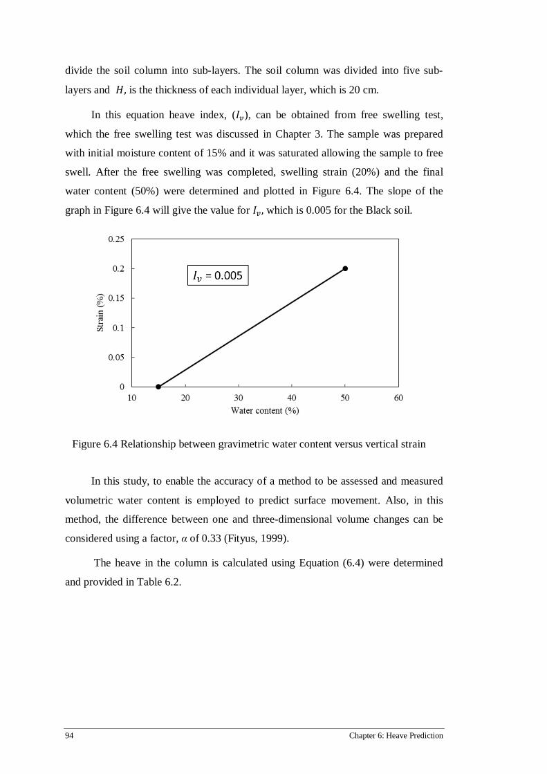
94 Chapter 6: Heave Prediction
divide the soil column into sub-layers. The soil column was divided into five sub-
layers and 𝐻, is the thickness of each individual layer, which is 20 cm.
In this equation heave index, (𝐼𝑣), can be obtained from free swelling test,
which the free swelling test was discussed in Chapter 3. The sample was prepared
with initial moisture content of 15% and it was saturated allowing the sample to free
swell. After the free swelling was completed, swelling strain (20%) and the final
water content (50%) were determined and plotted in Figure 6.4. The slope of the
graph in Figure 6.4 will give the value for 𝐼𝑣 , which is 0.005 for the Black soil.
Figure 6.4 Relationship between gravimetric water content versus vertical strain
In this study, to enable the accuracy of a method to be assessed and measured
volumetric water content is employed to predict surface movement. Also, in this
method, the difference between one and three-dimensional volume changes can be
considered using a factor, α of 0.33 (Fityus, 1999).
The heave in the column is calculated using Equation (6.4) were determined
and provided in Table 6.2.

Chapter 6: Heave Prediction 95
Table 6.2 Heave prediction results of Fityus and Smith (1998) method
Layer No.
Layer
thickness
(𝒄𝒄)
𝑰𝒗 𝜶 ∆𝒘 ∆𝑯
(𝒄𝒄)
1 20 0.005 0.33 40.69 1.53
2 20 0.005 0.33 40.44 1.53
3 20 0.005 0.33 39.99 1.51
4 20 0.005 0.33 39.72 1.50
5 20 0.005 0.33 38.97 1.47
Total heave 7.54
The estimated/predicted soil column heave by method-3 (Fityus and Smith, 1998)
is 75.4 mm and the maximum measured heave during the test in 56.7 mm. The results
indicate that the surface heave estimated by method-3 is 33% greater than what was
observed from the soil column. The possible reasons for this overestimation could
be:
• Boundary effects on the soil column
• Difference in the measured soil parameters
• No consideration of overburden pressure in estimating soil heave
6.5 SUMMARY
A comparison was made between the soil column heave data and selected
estimation methods to validate the accuracy of the prediction methods. All
parameters that were used for heave prediction such as; water content, suction and
swelling properties were determined and described in Chapter 3 and Chapter 5 in
details.
For all the selected methods, the ground movement was determined only for
the wetting cycle, since the equations are used for the worse scenario, normally
attributed to the wetting period (saturation) rather than the drying. The variation

96 Chapter 6: Heave Prediction
between the measured heave value obtained from the soil column and predicted
methods provided insights into the accuracy of estimation methods.
Table 6.3 Soil column and selected prediction methods heave results Heave estimation/prediction comparison
Soil column Aitchison
(1973)
Fredlund
(1983)
Fityus and
Smith (1998)
57.6 mm 195 mm 41.9 mm 75.4 mm
Table 6.3 shows that the Aitchison (1973) method overestimated ground heave
3.5 times greater than soil column heave results, while the Fityus and Smith (1998)
method gives only 33% overestimation. In contrast, the Fredlund (1983) prediction
method anticipated ground movement 26% less than the soil column experimental
result. The differences between heave prediction methods and actual heave data
might be caused as a result of boundary conditions effects, the difference in the
measured soil parameters, and the effect of overburden pressure. Thus, the soil
column results are recommended to be considered for ground movement studies on
the expansive soils.

97
Chapter 7: Conclusions and Recommendations
7.1 CONCLUSIONS
The extensive literature review carried out in this study revealed a need for an
instrumented soil column to investigate the behaviour of expansive soil in the
controlled laboratory environment to validate/develop methods for estimating
climate-induced surface ground movement in expansive soil. To fill this research
gap, four objectives were defined as given in Chapter 1. This section highlights the
achievement of each research objective.
(1) To develop an instrumented soil column to be used in laboratory conditions.
• As discussed in Chapter 4, an apparatus was designed and manufactured at
QUT comprising a soil column with 380 mm diameter and 1000 mm height.
The size of the column was determined to minimise the boundary effects of
the soil column tests. The soil column can be instrumented to measure soil
suction, soil moisture content, soil temperature, and sub-soil deformation at
five different levels along the height of the column. The column can be
wetted from the top or the bottom using water with the controlled head. The
soil in the column can be subjected to drying from the top. The following
devices/sensors were designed/manufactured and chosen to be used in the soil
column to investigate the behaviour of expansive soil subjected to wetting
and drying.
• A special type of settlement plate was designed and manufactured to measure
sub-soil deformation (shrink-swell) at different depths in the soil column. The
plate is attached to a vertical shaft and the top is attached to an LVDT to
measure the soil displacement at the depth of the plate. The shaft allows
movement along a sleeve to minimise the effects of soil friction above the
plate depth. The tops of both the shaft and the sleeve are maintained about
200 mm above the soil surface.
• A new tensiometer was designed and manufactured at QUT to measure low
soil suction (0 – 90 kPa). It consists of a water flushing system to remove
cavitated air bubbles in the ceramic cup while it is being used. The ceramic

98
cup, which is placed in the soil is connected to an acrylic block, which is
placed on the outside wall of the column. The acrylic block is designed to
connect a pressure transducer, with another connection required for flushing
the air bubbles in the ceramic cup. The ceramic cup and the acrylic block are
connected using two thin flexible tubes so that the ceramic cup can move in
the soil as it deforms without any damage to the tensiometer.
• To measure soil temperature and moisture, commercially available burial
thermocouple and moisture sensor (EC-5) were employed.
• To wet the soil by supplying water with constant head, a 20L Mariotte tank
was constructed.
• A custom-made logging system was developed to log all sensors at a
specified time interval.
The developed soil column and associated sensors/logging system fulfiled Objective
1 of this study.
(2) To investigate the performance of expansive soil layer subjected to wetting
and drying cycles.
• as explained in Chapter 4, the column was filled with a natural expansive soil
collected from the Ipswich area in South-East Queensland (Black soil). The
soil was prepared in the laboratory to achieve a uniform gravimetric moisture
content of 15%, and it was compacted into the column to achieve a dry
density of 1.2 g/cm3 and a soil height of 1000 mm. As the column was being
filled with soil, 23 sensors; five volumetric water content sensors, five
LVDTs attached to settlement plates, six thermocouples (one on the surface),
three tensiometers, three MPS-6 high suction sensors, and one relative
humidity sensor (just outside the column) were installed at five different
depths in the soil column. All the sensors/transducers were connected to a
data logger and logged every 1 min. The column was first subjected to
wetting from the top for four months ( August – November 2015) by
maintaining a small constant head using the Marriott bottle. The column was
then subjected to drying for four months ( December 2015 – March 2016) by
placing a heat lamp close to the soil surface. The responses of the sensors
presented in Chapter 5 were able to explain the wetting and drying of the soil

99
along the soil column depth. The results shown in Chapter 5 verified the
applicability the newly developed soil column to investigate the performance
of expansive soil subjected to wetting and drying. The following are some of
the key parameters measured /monitored/recorded by transducers:
• The soil surface heaved 56.7 mm during the four months of wetting. The
amount of heave decreases with depth in the column and at about 800 mm
depth consolidation was observed. Drying occurred only down to 150 mm
from the surface, and the surface shrunk about 10 mm from the final heave
level.
• As the wetting front moved down throughout the soil column, the sensors
responded accordingly. The initial volumetric water content of the soil was
18%, and it increased to 60% as the soil is saturated. The initial suction was
about 3000 kPa along the column, and this decreased almost to zero as the
soil saturated.
• During wetting, the temperature of the soil was about 21- 24°C throughout
the depth of the column. During drying, the temperature of the soil close to
the surface was about 37°C. The temperature gradually decreased with depth
and the temperature at 800 mm depth was about 25°C.
(3) To understand the limitations and issues of using instrumentation to measure
expansive soil parameters. Based on the monitored data during wetting and
drying of the soil column, the following issues were identified:
• The sensors buried in the soil should be allowed to move with the soil as it
moves. Otherwise, the sensor or/and the cable connected could be damaged.
• To measure the soil volumetric water content and soil suction, the
sensors/ceramic cups have to have proper contact with the soil. If these
sensors are not allowed to move with the soil (e.g. if the sensors are fixed to
the column wall), the soil movement due to shrink-swell will break the soil
contact with the sensors leading to misleading responses of the sensors.
• It is challenging to measure low suction (0 – 90 𝑘𝑃𝑘) in the long-term using
tensiometers. The tensiometer is the most accurate device to measure low
suction as it measures the suction directly using a ceramic filter to separate air

100
and water phases in soil. In long-term use, air cavities are formed in the water
in the tensiometer reservoir. Therefore, the tensiometers used in this type of
column tests should have a mechanism to remove cavitated air by flushing.
• It is important to calibrate all the sensors attached to the data logging system,
which is used in the soil column experiment, and it is important to perform
soil-specific calibration for volumetric water content sensors.
• Most volumetric water content sensors are sensitive to temperature and the
salinity of the water. Therefore, their readings should be corrected for
temperature and salinity.
• The method used to measure sub-soil deformation was very successful.
However, it is important to have a very rigid connection between the plate
and the shaft as the connection can be subjected to severe distress as the soil
shrink-swell.
(4) To validate some commonly used methods to estimate soil heave/characteristic
surface movement.
as detailed in Chapter 6, the three heave estimation methods: (i) Aitchison
(1973), (ii) Fredlund (1983), and (iii) Fityus and Smith (1998) were employed to
estimate the soil surface heave in the soil column during wetting. The estimated
surface heave from each method was compared with the measured surface heave
in the column (56.7 mm). The estimated surface heave in the column by
Aitchison (1973), Fredlund (1983), Fityus and Smith (1998) methods are 195 mm
(3.5 times overestimated), 41.9 mm (26% underestimated), and 75.4 mm (33%
overestimated), respectively. An unexpected structural failure will occur if the
underestimated heave predictions are used, while overestimation of heave will
increase construction costs. The instrumented soil column experiment provides
more accurate heave estimation during wetting and drying, which leads to more
cost-effective design and construction of structures on and in expansive soils.
This will provide a significant financial benefit to the community by reducing the
risk of failures and making structures more resilient to climate variations and
change.

101
7.2 RECOMMENDATIONS FOR FURTHER RESEARCH
Based on the outcomes and limitations encountered during the soil column test
conducted in this study, the following are recommended to improve the applicability
of the results of the instrumented soil column tests:
• Observe the performance of the newly developed tensiometer for long-term
measurment, before it is used in the soil column test.
• Perform instrumented soil column tests for number of wetting-drying cycles
for better understanding of the performance of expansive soil.
• Develop a numerical model to simulate the performance of the soil column
test.
• Improve the column test by taking the following into account:
* Place markers in the soil close to the acrylic wall so that they can be tracked
to obtain the sub-soil deformation.
* Use stronger material for the plate and the rod in the sub-soil deformation
measuring device so that it can not be damaged during soil shrink-swell.
* Calibrate the soil moisture sensors to investigate temperature effects.
Develop and apply temperature correction to the volumetric water content
values measured. It is better to use TDR probes to measure soil moisture in
the column as these sensors are not sensitive to temperature.


References 103
References
Adem, H. H., & Vanapalli, S. K. (2015). Review of methods for predicting in situ volume change movement of expansive soil over time. Journal of Rock Mechanics and Geotechnical Engineering, 7(1), 73-86.
Aitchison, G. (1965). Soil properties, shear strength and consolidation. Proceeding 6th nternational Conference Soil Mechanic Foundations Engineering.
Aitchison, G. and J. Holmes (1953). "Aspects of swelling in the soil profile." Aust. J. Appl. Sci 4: 244-259.
Aitchison, G.D. (1973). “The quantitative description of the stress-deformation behavior of expansive soils – preface to set of Papers.” Proceedings of the 3rd International Conference on Expansive Soils, 2, 79 – 82.
Alonso, E. E., Vaunat, J., & Gens, A. (1999). Modelling the mechanical behaviour of expansive clays. Engineering geology, 54(1), 173-183.
Allen, R. G., Pereira, L. S., Smith, M., Raes, D., & Wright, J. L. (2005). FAO-56 dual crop coefficient method for estimating evaporation from soil and application extensions. Journal of irrigation and drainage engineering, 131(1), 2-13.
Al-Rawas, A. A., Hago, A. W., & Al-Sarmi, H. (2005). Effect of lime, cement and Sarooj (artificial pozzolan) on the swelling potential of an expansive soil from Oman. Building and Environment, 40(5), 681-687.
Al-Shamrani, M. A. and A. W. Dhowian (2003). "Experimental study of lateral restraint effects on the potential heave of expansive soils." Engineering geology 69(1): 63-81.
Altmeyer, W.T. 1955. Discussion of engineering properties of expansive clays. Journal of the Soil Mechanics and Foundations Division, American Society of Testing and Materials, 81 (SM2) (1955), pp. 17–19.
AS2870, A. S. (2011). Residential Slabs and Footings. Standards Australia.

104 References
ASTM D5550-14, Standard Test Method for Specific Gravity of Soil Solids by Gas Pycnometer, ASTM International, West Conshohocken, PA, 2014.
ASTM D2487-11, Standard Practice for Classification of Soils for Engineering Purposes (Unified Soil Classification System), ASTM International, West Conshohocken, PA, 2011.
ASTM D4546-14, Standard Test Methods for One-Dimensional Swell or Collapse of Soils, ASTM International, West Conshohocken, PA, 2014,
ASTM D698-00a, Standard Test Methods for Laboratory Compaction Characteristics of Soil Using Standard Effort (12,400 ft-lbf/ft3 (600 kN-m/m3)), ASTM International, West Conshohocken, PA, 2000
Austroads (2004). Austroads research report: Model licence re-assessment procedure for older drivers: Stage 2 research (No. AP-R259 ⁄ 04). Sydney: Austroads.
Baumgarten, B., Jaehrig, J., Reemtsma, T., & Jekel, M. (2011). Long term laboratory column experiments to simulate bank filtration: factors controlling removal of sulfamethoxazole. Water Research, 45(1), 211-220.
Brackley, I. J. U. (1975). Interrelationship of the factors affecting heave of an expansive, unsaturated, clay soil. University of Natal.
Briaud, J.-L., Zhang, X., & Moon, S. (2003). Shrink test-water content method for shrink and swell predictions. Journal of Geotechnical and Geoenvironmental engineering, 129(7), 590-600.
Bowles, J.E. 1996. Foundation analysis and design. 5th ed. McGraw Hill Book Company, New York
Brooks, R. H. and A. T. Corey (1964). "Hydraulic properties of porous media and their relation to drainage design." Transactions of the ASAE 7(1): 26-0028.
Cameron, D. (2001). The extent of soil desiccation near trees in a semi-arid environment, Springer.

References 105
Chapman, D., Ahn, S., & Hunt, D. V. (2007). Investigating ground movements caused by the construction of multiple tunnels in soft ground using laboratory model tests. Canadian Geotechnical Journal, 44(6), 631-643.
Chen, Q., Shi, J., Liu, X., Wu, W., Liu, B., & Zhang, H. (2013). Simulation of estrogen transport and behavior in laboratory soil columns using a cellular automata model. Journal of contaminant hydrology, 146, 51-62.
Corey, A. T. (1994). Mechanics of immiscible fluids in porous media, Water Resources Publication.
Caunce, C. M. (2010). Effective road pavement design for expansive soils in Ipswich (Doctoral dissertation, University of Southern Queensland).
Day, R. W. (1994). Performance of slab-on-grade foundations on expansive soil. Journal of performance of constructed facilities, 8(2), 129-138.
Department of Environment and Resource Management (DERM) 2011. Salinity Management Handbook, Second edition, DNRQ97109 #28823, DERM, Brisbane.
Dhowian, A. W. (1990). "Heave prediction techniques and design consideration on expansive soils." J King Saud Univ Eng Sci 2: 355-377.
Donaldson, G. W. (1965). A study of level observations on buildings as indications of moisture movements in the underlying soil. National Building Research Institute.
Doris, J. J., Rizzo, D. M., & Dewoolkar, M. M. (2008). Forecasting vertical ground surface movement from shrinking/swelling soils with artificial neural networks. International journal for numerical and analytical methods in geomechanics, 32(10), 1229-1245.
El Sayed, S. and S. Rabbaa (1986). "Factors affecting behavior of expansive soils in the laboratory and field—a review." Geotechnical Engineering 17(1): 89-107.

106 References
Fall, M., & Sarr, A. M. (2006). Geotechnical characterization of expansive soils and their implications in ground movements in Dakar. Bulletin of Engineering Geology and the Environment, 66(3), 279-288. doi:10.1007/s10064-006-0070-1
Fityus, S. and D. Smith (1998). A simple model for the prediction of free surface movements in swelling clay profiles. Proceedings, 2nd International Conference on Unsaturated Soils, Beijing, China.
Fityus, S. (1999). A soil moisture based method of estimating ys. Paper presented at the Proceedings 8th Australia New Zealand Conference on Geomechanics: Consolidating Knowledge.
Fredlund, D. (1969). Consolidometer test procedural factors affecting swell properties. Proceedings of the Second International Conference on Expansive Clay Soils, Texas A & M Press, College Station, TX.
Fredlund, D. (1983). Prediction of ground movements in swelling clays. Presentation of the 31st Annual Soil Mechanics and Foundation Engineering Conference, Minneapolis, Minn. American Society of Civil Engineers, New York.
Fredlund, D. G., & Rahardjo, H. (1993). Soil mechanics for unsaturated soils: John Wiley & Sons.
Fredlund, D. G. and A. Xing (1994). "Equations for the soil-water characteristic curve." Canadian Geotechnical Journal 31(4): 521-532.
Fredlund, D. G., Xing, A., & Huang, S. (1994). Predicting the permeability function for unsaturated soils using the soil-water characteristic curve. Canadian Geotechnical Journal, 31(4), 533-546.
Fredlund, D. (1995). The prediction of heave in expansive soils. Proceedings of the Canada–Kenya Symposium on Unsaturated Soil Behavior and Applications.
Fredlund, D.G. (1996). The Emergence of Unsaturated Soil Mechanics. The Fourth
Spencer J. Buchanan Lecture, College Station, Texas, A & M University Press, p. 39.

References 107
Fredlund, D. G., Schanz, T., & Lins, Y. (2009). Modified pressure plate apparatus and column testing device for measuring SWCC of sand.
Fredlund, D. G., Rahardjo, H., & Fredlund, M. D. (2012). Unsaturated soil mechanics in engineering practice: John Wiley & Sons.
Gardner, W. (1958). "Some steady-state solutions of the unsaturated moisture flow equation with application to evaporation from a water table." Soil science 85(4): 228-232.
Gibbs, H. J. (1973). "Use of consolidometer for measuring expansion, potential of soils." Publication of: Wyoming University 1(Workshop Proceedings).
Gizienski, S. and J. Lee (1965). Comparison of laboratory swell tests to small scale field. International Research and Engineering Conference on Expansive Clay Soils.
Hamberg, D. J., & Nelson, J. D. (1984). Prediction of floor slab heave. In Fifth International Conference on Expansive Soils 1984: Preprints of Papers (p. 137). Institution of Engineers, Australia.
Hardy, R. (1965). "Identification and performance of swelling soil types." Canadian Geotechnical Journal 2(2): 141-153.
Holtz, W. G. and H. J. Gibbs (1956). "Engineering properties of expansive clays." Transactions of the American Society of Civil Engineers 121(1): 641-663.
Hor, B., Caudron, M., & Marwan, A. (2011). Experimental analysis of the impact of ground movements on surface structure. Paper presented at the 64. Canadian geotechnical conference-14. Pan-America conference on soil mechanics and geotechnical engineering.
Isbell, R. F., McDonald, W. S., & Ashton, L. J. (1997). Concepts and rationale of the Australian soil classification.
Isbell, R. (2016). The Australian soil classification. CSIRO publishing.

108 References
Jahangir, E., Deck, O., & Masrouri, F. (2012). Estimation of ground settlement beneath foundations due to shrinkage of clayey soils. Canadian Geotechnical Journal, 49(7), 835-852.
Jennings, J., Firth, R., Ralph, T., & Nagar, N. (1973). An improved method for predicting heave using the oedometer test. Paper presented at the Proceedings of the 3rd International Conference on Expansive Soils.
Jennings, J. and K. Knight (1957). "The prediction of total heave from the double oedometer test." Transactions of the South African Institute of Civil Engineering 7: 285-291.
Johnson, L. t. and D. Snethen (1978). "Prediction of potential heave of swelling soils." Geotechnical Testing Journal 1(3): 117-124.
Jones, D.E. and Holtz, W.G., 1973. Expansive soils - the hidden disaster. Civ. Eng., ASCE, 43 (CE8): 49.
Jones, L. D., & Jefferson, I. (2012). Expansive soils (pp. 413-441). ICE Publishing.
Jones, D. E., & Jones, K. A. (1987). Treating expansive soils. Civil Engineering ASCE, 57(8), 62-65.
Justo, J., Delgado, A., & Ruiz, J. (1984). The influence of stress-path in the collapse-swelling of soils at the laboratory. Paper presented at the Fifth International Conference on Expansive Soils 1984: Preprints of Papers.
Kariuki, P. C., & Van Der Meer, F. (2004). A unified swelling potential index for expansive soils. Engineering geology, 72(1), 1-8.
Ke, J., Gin, K. Y. H., Tan, L. H., & Reinhard, M. (2012). Fate of endocrine-disrupting and pharmaceutically active substances in sand columns fed with secondary effluent. Journal of Environmental Engineering.
Kim, D. H., Kim, S. K., & Gratchev, I. (2013). Unsaturated seepage behavior study using soil column test.

References 109
Kumar, N. (1984). Review of common design and construction practices on expansive soils in Colorado. Fifth International Conference on Expansive Soils 1984: Preprints of Papers, Institution of Engineers, Australia.
Lambe, T. W. and R. V. Whitman (1959). The role of effective stress in the behavior of expansive soils, Soil Engineering Division, Massachusetts Institute of Technology.
Leao, S. (2014). "Mapping potential risk for housing damage from ground movement due to climate change." International Journal of Environmental Science and Development 5(4): 387.
Lee, K., & Rowe, R. (1991). An analysis of three-dimensional ground movements: the Thunder Bay tunnel. Canadian Geotechnical Journal, 28(1), 25-41.
Lehmann, P., Stauffer, F., Hinz, C., Dury, O., & Flühler, H. (1998). Effect of hysteresis on water flow in a sand column with a fluctuating capillary fringe. Journal of Contaminant Hydrology, 33(1), 81-100.
Leong, E. C. and H. Rahardjo (1997). "Review of soil-water characteristic curve equations." Journal of Geotechnical and Geoenvironmental engineering 123(12): 1106-1117.
Lewis, J., & Sjöstrom, J. (2010). Optimizing the experimental design of unsaturated soil columns. Paper presented at the Proceedings of the 19 th World Congress of Soil Science “Soil Solutions for a Changing World”. Brisbane (Australia).
Lory, J. (2015). "Structure of clay minerals." from http://www.thedirtdoctors.com/whats-the-crack-the-science-of-clay-related-subsidence/.
Lu, N. and W. J. Likos (2006). "Suction stress characteristic curve for unsaturated soil." Journal of Geotechnical and Geoenvironmental engineering 132(2): 131-142.
Lytton, R. (1977). Foundations in expansive soils, McGraw-Hill.

110 References
Mali, N., Urbanc, J., & Leis, A. (2007). Tracing of water movement through the unsaturated zone of a coarse gravel aquifer by means of dye and deuterated water. Environmental geology, 51(8), 1401-1412.
Masia, M. J., Totoev, Y. Z., & Kleeman, P. W. (2004). Modeling expansive soil movements beneath structures. Journal of Geotechnical and Geoenvironmental engineering, 130(6), 572-579.
Matyas, E. (1969). Some properties of two expansive clays from western Canada. Proceedings of the 2nd International Conference on Expansive Soils. Texas A&M University, College Station, Texas.
McKeen, R. G. (1992). A model for predicting expansive soil behavior. Proc., 7th Int. Conf. on Expansive Soils, ASCE Reston, VA.
McKenzie, N., Jacquier, D., Isbell, R., & Brown, K. (2004). Australian soils and landscapes. An illustrated compendium.,(CSIRO Publishing: Collingwood, Vic.).
McWhorter, D. B. and D. K. Sunada (1977). Ground-water hydrology and hydraulics, Water Resources Publication.
Mitchell, P. and D. Avalle (1984). A technique to predict expansive soil movements. Fifth International Conference on Expansive Soils 1984: Preprints of Papers, Institution of Engineers, Australia.
Mitchell JK, Soga K (2005) Fundamentals of soil behaviour. 3rd edn. Willy. New York.
Mualem, Y. (1976). "A new model for predicting the hydraulic conductivity of unsaturated porous media." Water resources research 12(3): 513-522.
Nelson, J. D., Reichler, D. K., & Cumbers, J. M. (2006). Parameters for heave prediction by oedometer tests. Paper presented at the Unsaturated Soils 2006.
Nelson, J. D., & Miller, D. J.(1992). Expansive Soils: Problems and Practice in Foundation and Pavement Engineering. John Wiley & Sons. New York

References 111
Noble, C. A. (1966). "Swelling measurements and prediction of heave for a lacustrine clay." Canadian Geotechnical Journal 3(1): 32-41.
Pitt, W. G. (1982). Correlation Between the Real Behaviour and the Theoretical Design of Residential Raft Slabs, Swinburne Institute of Technology.
Porter, A. A. and J. D. Nelson (1980). Strain controlled testing of expansive soils. Expansive Soils, ASCE.
Puppala, A. J., Punthutaecha, K., & Vanapalli, S. K. (2006). Soil-water characteristic curves of stabilized expansive soils. Journal of Geotechnical and Geoenvironmental Engineering, 132(6), 736-751.
Puppala, A. J., & Chittoori, B. C. (2012). Transportation infrastructure settlement and heave distress: challenges and solutions. Journal of Zhejiang University SCIENCE A, 13(11), 850-857.
Radford, B., Gibson, G., Nielsen, R., Butler, D., Smith, G., & Orange, D. (1992). Following practices, soil water storage, plant-available soil nitrogen accumulation and wheat performance in South West Queensland. Soil and Tillage Research, 22(1), 73-93.
Rajeev, P., Chan, D., & Kodikara, J. (2012). Ground–atmosphere interaction modelling for long-term prediction of soil moisture and temperature. Canadian Geotechnical Journal, 49(9), 1059-1073.
Ranganatham, B. and B. Satyanarayana (1965). A rational method of predicting swelling potential for compacted expansive clays. Proceedings of the 6th International Conference on Soils Mechanics and Foundation Engineering, Montreal.
Rao, R. R., Rahardjo, H., & Fredlund, D. G. (1988). Closed-form heave solutions for expansive soils. Journal of geotechnical engineering, 114(5), 573-588.
Reed, R. F., & Kelley, M. (2000). Impact of climatic variation on design parameters for slab on ground foundations in expansive soils. Geotechnical Special Publication, 435-455.

112 References
Rees, S. W., & Thomas, H. R. (1993). Simulating seasonal ground movement in unsaturated clay. Journal of geotechnical engineering, 119(7), 1127-1143.
Reins, J. D., & Volz, J. J. (2013). Monitoring and mitigation of movements affecting foundations on expansive soils in Colorado. Journal of Performance of Constructed Facilities, 27(6), 731-736.
Richards, B. (1965). Measurement of free energy of soil moisture by the psychrometric technique, using thermistors.
Richards, B., Peter, P., & Emerson, W. (1983). The effects of vegetation on the swelling and shrinking of soils in Australia. Géotechnique, 33(2), 127-139.
Roads, M. (2000). 4-seeable futures: transport portfolio scenario based planning for the Queensland Department of Transport and the Queensland Department of Main Roads, 2000-2025.
Rogers, J. D., Olshansky, R., & Rogers, R. B. (1993). Damage to foundations from expansive soils. Claims People, 3(4), 1-4.
Roger, D. (2008). "Natural Slope Creep." Missouri University of Science and Technology Courses, from; http://web.mst.edu/~rogersda/umrcourses/ge441/online_lectures/mass_grading/GE441-Lecture1-2.pdf.
Ruan, M. (1999). Continuous simulation of CSO emissions. Urban water, 1(3), 201-205.
Saber, A., Sterling, R., & Nakhawa, S. A. (2003). Simulation for ground movements due to pipe bursting. Journal of infrastructure systems, 9(4), 140-144.
Sattler, P., & Fredlund, D. (1991). Numerical modelling of vertical ground movements in expansive, soils. Canadian Geotechnical Journal, 28(2), 189-199.
Schneider, G. L. and A. R. Poor (1974). The prediction of soil heave and swell pressures developed by an expansive clay, University of Texas.

References 113
Seed, H., Woodward Jr, R., & Lundgren, R. (1962). Prediction of swelling potential for compacted clays. Journal of the soil mechanics and foundations division, 88(3), 53-88.
Sentenac, P., Lynch, R., & Bolton, M. (2001). Measurement of a side-wall boundary effect in soil columns using fibre-optics sensing. International Journal of Physical Modelling in Geotechnics, 1(4), 35-41.
Shanker, N. B., Rao, A. S., & Swamy, A. (1982). Swelling behaviour of undisturbed and remoulded samples of black cotton clay. Indian Geotechnical Journal, 12(2).
Shannon, B., Gallage, C., & Kodikara, J. (2010). Experimental modelling of coupled water flow and associated movements in swelling soils. Paper presented at the Proceedings from the 3rd International Conference on Problematic Soils.
Shuai, F. (1996). "Simulation of swelling pressure measurements on expansive soils."
Siemens, J., Huschek, G., Walshe, G., Siebe, C., Kasteel, R., Wulf, S., & Kaupenjohann, M. (2010). Transport of pharmaceuticals in columns of a wastewater-irrigated Mexican clay soil. Journal of environmental quality, 39(4), 1201-1210.
Skempton, A. W. (1961). Horizontal stresses in an overconsolidated Eocene clay. In Proc. 5th Int. Conf. Soil Mech (Vol. 1, pp. 351-357).
Snethen, D. R. (1980). Characterization of expansive soils using soil suction data. Expansive Soils, ASCE.
Standard, A. 1289.3. 6.1, Methods of testing soils for engineering purposes - Soil classification tests - Determination of the particle size distribution of a soil - Standard method of analysis by sieving.
Standard, A. 1289.3.6.3-2003. Methods of testing soils for engineering purposes - Soil classification tests - Determination of the particle size distribution of a soil - Standard method of fine analysis using a hydrometer.

114 References
Standard, A. 1289.3.1.1-2009. Methods of testing soils for engineering purposes - Soil classification tests - Determination of the liquid limit of a soil - Four point Casagrande method
Standard, A. 1289.3.2.1-2009. Methods of testing soils for engineering purposes - Soil classification tests - Determination of the plastic limit of a soil - Standard method
Standard, A. 1289.3.4.1-2009. Methods of testing soils for engineering purposes - Soil classification tests - Determination of the linear shrinkage of a soil - Standard method
Stauffer, F., & Kinzelbach, W. (2001). Cyclic hysteretic flow in porous medium column: model, experiment, and simulations. Journal of Hydrology, 240(3), 264-275.
Van Genuchten, M. T. (1980). "A closed-form equation for predicting the hydraulic conductivity of unsaturated soils." Soil science society of America journal 44(5): 892-898.
Vanapalli, S., Fredlund, D., Pufahl, D., & Clifton, A. (1996). Model for the prediction of shear strength with respect to soil suction. Canadian Geotechnical Journal, 33(3), 379-392.
Vanapalli, S., Lu, L., & Oh, W. (2010). Estimation of swelling pressure and 1-D heave in expansive soils. Paper presented at the Proceedings of the 5th International Conference on Unsaturated Soils, Barcelona, Spain, September.
Vijayvergiya, V. and O. Ghazzaly (1973). Prediction of swelling potential for natural clays. Proceedings of the Third International Conference on Expansive Clay Soils.
Voegelin, A.C. Scheinost, K. Buhlmann, K. Barmettler, R. Kretzschmar (2002). Slow formation and dissolution of Zn precipitates in soil: a combined column-transport and XAFS study. Environ. Sci. Technol., 36 (2002), pp. 3749-3754.
Wagle, D., Gad, E., Sivanerupan, S., & Wilson, J. L. (2013). Damage potential to residential structures due to ground movement.

References 115
Walsh, P. F. (1978). The analysis of stiffened rafts on expansive clays.
Weston, D. (1980). Expansive roadbed treatment for Southern Africa. Proceedings of the Conference on Expansive Soils ASCE, Denver, Colo., June 16-18, 1980.
Zapata, C. E. (1999). Uncertainty in soil-water-characteristic curve and impacts on unsaturated shear strength predictions. Arizona State University.
Zhang, L. W., & Wang, R. (2002). Research on status quo of anchorage theory of rock and soil. ROCK AND SOIL MECHANICS-WUHAN-, 23(5; ISSU 79), 627-631.
Zumrawi, M. M. (2016). Construction Problems of Light Structures Founded on Expansive Soils in Sudan.