Develop and prototype codegeneration techniques for aclause-based GPU

Johan Ju, Niklas Jonsson

MASTER’S THESIS | LUND UNIVERSITY 2017

Department of Computer ScienceFaculty of Engineering LTH

ISSN 1650-2884 LU-CS-EX 2017-08

Develop and prototype code generationtechniques for a clause-based GPU

Johan Jujohanj93@gmail.com

Niklas Jonssonniklasandersjonsson@gmail.com

June 2, 2017

Master’s thesis work carried out at ARM Sweden AB.

Supervisors: Jonas Skeppstedt, Jonas.Skeppstedt@cs.lth.seDmitri Ivanov, Dmitri.Ivanov@arm.comMarkus Lavin, Markus.Lavin@arm.com

Examiner: Krzysztof Kuchcinski, Krzysztof.Kuchcinski@cs.lth.se

Abstract

Processors grow more and more complex, even more so in the field of GPUs,where the instruction set, in general, is not publicly available. This enablesthem to change more rapidly than CPUs, since backwards compatibility is notan issue. In this thesis multiple approaches are investigated for code generationfor a clause-based GPU. An optional pre-scheduler is implemented, togetherwith two approaches for register allocation and one post-scheduler. It is foundthat a pre-scheduler can lower the register pressure considerably which makesa major impact on register allocation. The differences between the two registerallocators is minimal and they can be considered to be equal.

Keywords: code generation, gpu, register allocation, instruction scheduling

2

Acknowledgements

We would like to thank ARM for giving us the opportunity to do our thesis in coopera-tion with them. Furthermore, we would like to thank our supervisors at ARM, MarkusLavin and Dmitri Ivanov, going out of their way to support us with everything from im-plementation details to thesis writing. We would also like to thank Jonas for his supportand comments, both for this thesis but also the preceding literature study that is the basisfor the theorical parts of this thesis. Lastly, both of the authors would like to thank theirrespective family and friends for their love and support.

3

4

Contents

1 Introduction 71.1 Background . . . . . . . . . . . . . . . . . . . . . . . . . . . . . . . . . 71.2 Bifrost architecture . . . . . . . . . . . . . . . . . . . . . . . . . . . . . 71.3 Problem . . . . . . . . . . . . . . . . . . . . . . . . . . . . . . . . . . . 91.4 Goals and Limitations . . . . . . . . . . . . . . . . . . . . . . . . . . . . 9

2 Theory 112.1 SSA Form . . . . . . . . . . . . . . . . . . . . . . . . . . . . . . . . . . 122.2 Register Allocation . . . . . . . . . . . . . . . . . . . . . . . . . . . . . 12

2.2.1 Linear Scan . . . . . . . . . . . . . . . . . . . . . . . . . . . . . 132.2.2 Linear Scan on SSA form . . . . . . . . . . . . . . . . . . . . . 132.2.3 Chaitin’s algorithm . . . . . . . . . . . . . . . . . . . . . . . . . 132.2.4 Graph coloring on SSA form . . . . . . . . . . . . . . . . . . . . 14

2.3 Instruction Scheduling . . . . . . . . . . . . . . . . . . . . . . . . . . . 142.3.1 List Scheduling . . . . . . . . . . . . . . . . . . . . . . . . . . . 152.3.2 Modulo Scheduling . . . . . . . . . . . . . . . . . . . . . . . . . 15

2.4 Previous work . . . . . . . . . . . . . . . . . . . . . . . . . . . . . . . . 16

3 Approach 193.1 Pre-scheduler . . . . . . . . . . . . . . . . . . . . . . . . . . . . . . . . 20

3.1.1 Model . . . . . . . . . . . . . . . . . . . . . . . . . . . . . . . . 213.1.2 Heuristics (priority function) . . . . . . . . . . . . . . . . . . . . 21

3.2 Live range-based register allocation . . . . . . . . . . . . . . . . . . . . 223.2.1 Shuffle insertion . . . . . . . . . . . . . . . . . . . . . . . . . . 233.2.2 Wide variables as arguments . . . . . . . . . . . . . . . . . . . . 25

3.3 Coupled register allocator . . . . . . . . . . . . . . . . . . . . . . . . . . 253.3.1 Spilling . . . . . . . . . . . . . . . . . . . . . . . . . . . . . . . 253.3.2 Coloring . . . . . . . . . . . . . . . . . . . . . . . . . . . . . . 26

3.4 Post scheduling . . . . . . . . . . . . . . . . . . . . . . . . . . . . . . . 26

5

CONTENTS

4 Results 294.1 Metrics . . . . . . . . . . . . . . . . . . . . . . . . . . . . . . . . . . . 30

5 Discussion 335.1 Coupled register allocator . . . . . . . . . . . . . . . . . . . . . . . . . . 335.2 Unified Scheduling and Register Allocation . . . . . . . . . . . . . . . . 345.3 Live range based register allocator . . . . . . . . . . . . . . . . . . . . . 365.4 Post scheduling . . . . . . . . . . . . . . . . . . . . . . . . . . . . . . . 36

6 Conclusions 396.1 Future work . . . . . . . . . . . . . . . . . . . . . . . . . . . . . . . . . 39

Bibliography 41

Appendix A Test suite listing 1 45

Appendix B Test suite listing 2 49

6

Chapter 1Introduction

1.1 BackgroundThe thesis is carried out at ARM, a company that licences their hardware designs (intel-lectual property) to hardware manufacturers for use in System on Chips (SoCs). The officein Lund, where the thesis project has been carried out, is a part of the Media ProcessingGroup which is responsible for developing the Mali GPU family as well as Video Process-ing Units (VPUs) and Display Processing Units (DPUs), together with their accompanyingdrivers. Like most modern GPUs, Mali features a programmable pipeline where some ofthe stages run shader programs whilst others are fixed in hardware. An application mayeither submit a shader written in a high level shader language which the driver needs tocompile at runtime or a pre-compiled binary that the driver simply runs on the GPU. ARMhas recently released a new hardware architecture called Bifrost and our task is to designa code generator to explore different approaches to code generation for shaders in Bifrost.

1.2 Bifrost architectureThe compiler in this thesis is targeting ARM’s Bifrost architecture which is their latestGPU design [19]. Bifrost is a scalar architecture where arithmetic instructions use scalar32-bit registers as operands. This is different from the previous Midgard architecture whichuses wide vector register operands. There are two arithmetic functional units in Bifrostcalled FMA and ADD/SF shown in fig. 1.1. Some instructions can only execute in theFMA unit while others can only execute in the ADD/SF unit. But there are also instructionsthat can execute in both units.

Instructions are represented in pairs so that every instruction pair has an instructionfor each unit. Those instruction pairs are then inserted into a clause that can contain mul-tiple instruction pairs. A clause is a series of instruction pairs that can execute without

7

1. Introduction

Figure 1.1: Arithmetic functional units

Figure 1.2: Use of bypass register

switching thread.The clause can be of varying length. Every clause can only contain oneinstruction with uncertain latency e.g. memory access. Within a clause, instructions canfetch data from a temporary (bypass) register that contains the result from the latest exe-cuted instruction see fig. 1.2. One benefit of using the temporary register is that a slot inthe register file does not always need to be overwritten. Temporary registers can be seenas forwarding the result and can’t hold the value for an extended period of time.

Furthermore, the ISA (Instruction Set Architecture) of Bifrost supports wide instruc-tions for memory access, i.e. instruction that write to more than one register. Whilst theseare optional in general, the efficiency of code is generally increased if they are used. Takefor example a load instruction that reads from memory and writes to a register. Instead ofseveral such loads we can use a wide load that writes to several registers, saving one ormore memory accesses.

8

1.3 Problem

1.3 ProblemThe general problem is the classical task of combining instruction scheduling and registerallocation to produce effective code. But the goal for scheduling for GPUs is differentto traditional CPU scheduling. Because of the nature of graphical workloads, GPUs aredesigned to switch threads with little overhead. This feature is used to hide memory accesslatency as other threads can run instead of stalling. The Bifrost architecture introducessome important features that will affect the scheduler considerably. Firstly, as describedabove, there are clauses that bind together instructions with fixed latency that they canexecute all the way without worrying about switching threads. The compiler is solelyresponsible for scheduling the clauses and allocating the bypass registers. There is alsosome benefit of keeping values in adjacent registers which needs to be considered by theregister allocator. Together with this there are several constraints on how constant may beencoded into instructions, how clause execution may be interleaved, specific features ofgraphics hardware etc. that the scheduler and register allocator have to take into accountwhen attempting to produce efficient code.

1.4 Goals and LimitationsThe goal of this thesis/report is to develop and prototype code generation techniques forthe Bifrost architecture. It will also present whether the traditional strategies for doingregister allocation and instruction selection can be applied effectively to the architectureand if not, how one should perform them differently to generate code that performs well.For this purpose, a compiler back-end is developed consisting of instruction selection, anoptional pre-scheduler, register allocation, post-scheduling and instruction emission. Thisis further detailed in chapter 3.

As for author contribution to this thesis, Niklas was mainly responsible for the sectionson Graph Coloring algorithms, Modulo scheduling, section 3.2, section 3.4, whilst Johanwrote most of the sections on Linear Scan, List Scheduling, section 3.1, section 3.3 andsection 5.2.

9

1. Introduction

10

Chapter 2Theory

Most compilers can be divided into three parts: front-end, middle-end and back-end. Thefront-end handles parsing of the input program, checking so that it follows the applicablesyntax rules and translating the input program into some form of intermediate representa-tion (IR) that is used for the rest of the compilation. The middle-end performs optimizationthat are not architecture-specific, e.g. dead code elimination. The back-end (also knownas code generator) translates the IR to to the assembly required for the target platform, thusthe back-end is architecture-specific. As this thesis is mainly concerned with the back-end,the front-end and middle-end are not described further.

Up until the back-end, variables have been used to hold values but one task of theback-end is to map these to hardware registers and memory locations. In general, thereare not enough hardware registers so that each register is only assigned to one variable,instead variables need to share registers. A variable is assigned to a register and whilstthat variable (or rather the value it represents) is still needed the register is allocated tothat variable only. The duration a variable is needed is called its lifetime or live range,and the variable is said to be live during this. The amount of live variables with respect toit’s width at a specific point in the program is denoted the register pressure. If there arenot enough free hardware registers to hold all variables, variables need to be spilled, i.e.stored in memory. Spilling a variable is usually done by storing it in memory directly afterits definition and loading it before each uses. Each load is replaced with different variable,thus the lifetime of the variable is shortened to only small intervals and register pressureis reduced.

The back-end may also perform instruction scheduling in order to increase the perfor-mance of the program. Some instructions may have latency, i.e. that their results are onlyavailable after a number of cycles and thus unrelated instructions may be executed in themeantime. Depending on which instructions have been previously scheduled, no unrelatedinstructions may be available and the scheduler might have to insert NOP (no-operation)instructions, effectively stalling the processing unit, and wasting cycles that may have beenused to execute instructions. Scheduling unrelated instructions increases the register pres-

11

2. Theory

y ←

y ←y ←

← y

(a)

y1 ←

y3 ←y2 ←

y4 ← φ(y2, y3)← y4

(b)

Figure 2.1: Example program, not on SSA-form (a) and on SSA-form (b)

sure and thus might lead to spilling. For the architecture investigated in this thesis, anothergoal of the scheduler is to allocate instructions to the functional units so as to keep themas busy as possible. The classical approaches to code generation and their application to ageneralized Bifrost architecture were explored in a report [11]. The relevant parts will bereused in this chapter.

2.1 SSA FormA program is said to be on SSA-form if each variable is only defined once, and each vari-able is defined before being used. SSA-from simplifies several compiler optimizationsand most modern compilers make use of it today [17]. Converting a program to SSA-formusually involves renaming any re-definitions of a variable and changing the subsequentuses appropriately. As illustrated in fig. 2.1a, this introduces a problem when a use can bereached from two different definitions, depending on which control flow path is taken dur-ing execution. The solution to this is to introduce φ-functions, an function which producesa different variable depending on which predecessor was executed. The same program canbe seen in fig. 2.1b, now on SSA-form, with φ-functions where appropriate.

2.2 Register AllocationChaitin described [5] how register allocation process can be modeled as graph coloring.Graph coloring is the problem of, given a graph, coloring it such that no two neighbouringnodes have the same color. His algorithm has been the basis of several other papers, whichaim to improve upon it [3, 7]. In general graph coloring is NP-complete (given Chaitin’sassumptions) and as such, heuristics have to be used to solve register allocation withinreasonable time. Among them are Linear scan [16] and Chaitin’s algorithm, describedfurther below. In some cases we can make assumptions about the graph which makes itpossible to color it in polynomial time. This is further described in section 2.2.4.

12

2.2 Register Allocation

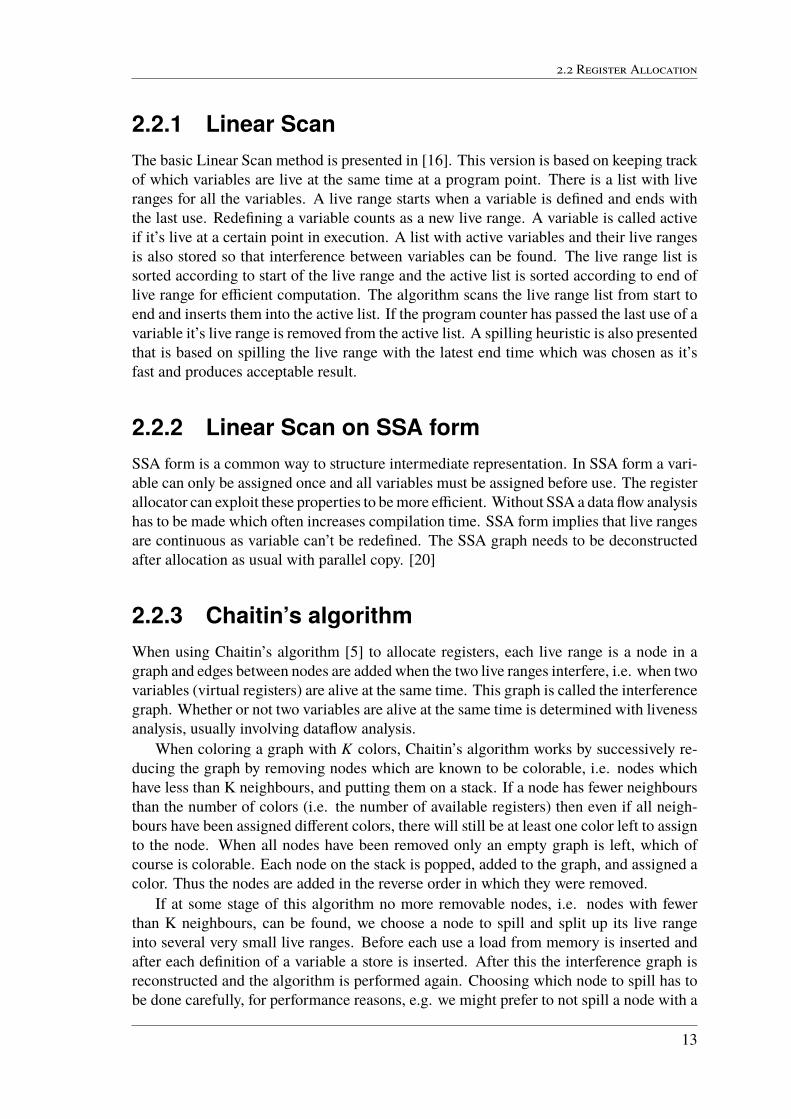
2.2.1 Linear ScanThe basic Linear Scan method is presented in [16]. This version is based on keeping trackof which variables are live at the same time at a program point. There is a list with liveranges for all the variables. A live range starts when a variable is defined and ends withthe last use. Redefining a variable counts as a new live range. A variable is called activeif it’s live at a certain point in execution. A list with active variables and their live rangesis also stored so that interference between variables can be found. The live range list issorted according to start of the live range and the active list is sorted according to end oflive range for efficient computation. The algorithm scans the live range list from start toend and inserts them into the active list. If the program counter has passed the last use of avariable it’s live range is removed from the active list. A spilling heuristic is also presentedthat is based on spilling the live range with the latest end time which was chosen as it’sfast and produces acceptable result.

2.2.2 Linear Scan on SSA formSSA form is a common way to structure intermediate representation. In SSA form a vari-able can only be assigned once and all variables must be assigned before use. The registerallocator can exploit these properties to be more efficient. Without SSA a data flow analysishas to be made which often increases compilation time. SSA form implies that live rangesare continuous as variable can’t be redefined. The SSA graph needs to be deconstructedafter allocation as usual with parallel copy. [20]

2.2.3 Chaitin’s algorithmWhen using Chaitin’s algorithm [5] to allocate registers, each live range is a node in agraph and edges between nodes are added when the two live ranges interfere, i.e. when twovariables (virtual registers) are alive at the same time. This graph is called the interferencegraph. Whether or not two variables are alive at the same time is determined with livenessanalysis, usually involving dataflow analysis.

When coloring a graph with K colors, Chaitin’s algorithm works by successively re-ducing the graph by removing nodes which are known to be colorable, i.e. nodes whichhave less than K neighbours, and putting them on a stack. If a node has fewer neighboursthan the number of colors (i.e. the number of available registers) then even if all neigh-bours have been assigned different colors, there will still be at least one color left to assignto the node. When all nodes have been removed only an empty graph is left, which ofcourse is colorable. Each node on the stack is popped, added to the graph, and assigned acolor. Thus the nodes are added in the reverse order in which they were removed.

If at some stage of this algorithm no more removable nodes, i.e. nodes with fewerthan K neighbours, can be found, we choose a node to spill and split up its live rangeinto several very small live ranges. Before each use a load from memory is inserted andafter each definition of a variable a store is inserted. After this the interference graph isreconstructed and the algorithm is performed again. Choosing which node to spill has tobe done carefully, for performance reasons, e.g. we might prefer to not spill a node with a

13

2. Theory

lot of uses, since this would incur several loads but prefer a variable with a long live range.With this in mind the algorithm usually terminates within a few iterations.

Chaitin’s algorithm also includes a coalescing stage where the nodes of the argumentand the result of a copy instruction are merged in the interference graph (if they do notalready interfere). The new node might have more than K neighbours though, which mightmake the graph uncolorable. Coalescing without regarding the colorability of the graphis called aggressive coalescing and it is what Chaitin employs [5]. Briggs et al. propose amore conservative approach [3]. George & Appel believes this to be too conservative andpropose a solution that performs a more aggressive coalescing [7].

2.2.4 Graph coloring on SSA formHack et al. [10] describe a novel way to perform graph coloring register allocation. Ifwe can assume the code is in SSA form as described by Cytron et al. [6], we can utilizethe fact that the interference graph of an SSA-program is chordal. Since the time it takesto color chordal graphs is quadratic, the time it takes to find the chromatic number, thenumber of colors needed to color a graph, is also quadratic.

Hack proposes an algorithm where all the necessary spilling is done first by computingthe chromatic number for the graph and then, if it is not already colorable with the availableregisters, the necessary variables are spilled using some heuristic (since the problem ofspilling is NP-complete). Here Hack uses Belady’s MIN algorithm [1] for basic blockspilling but others may be used as well. After this stage the interference graph is colorableaccording to an order defined by the dominance relation of the program, which is provento be an optimal coloring by Hack.

After the coloring phase, coalescing is performed using φ-functions. Hack describesan approximation to optimal coalescing (since this also is NP-complete): Maximize thenumber of φ-operands that share color with the destination of the φ-function. This willminimize the number of moves this φ-function will result in but does not guarantee optimalcoalescing in the global sense. This does not change the colorability of the interferencegraph - no additional register demand arises and thus no iteration is needed (as might bethe case with Chaitin’s and it’s derivatives) and the algorithm terminates.

Pereira F. published a technical report [14] detailing the implementation of a registerallocator on SSA-form. It differs from Hack’s on several points but it retains the same basicstructure with pre-spilling, coloring and coalescing. The main difference is that Pereira’salgorithm allows φ-virtuals to be mapped to memory, giving the compiler extra freedomto choose values to spill, but requires a more complex φ-deconstruction algorithm. Otherdifferences include: the global register coalescing heuristics, the handling of pre-coloredvariables and the spilling heuristics.

2.3 Instruction SchedulingInstruction scheduling is the process of rearranging the order of instructions to minimizepipeline stalls, which is usually done by distancing a producer and a consumer of a valueas much as needed. Finding an optimal schedule is NP-complete [17].

14

2.3 Instruction Scheduling

When doing instruction scheduling the algorithm has to address two main issues. Firstone is to consider how to express the constraints so that the result is correct, i.e. anydependencies between instructions have to be taken into account. Then the algorithmmust determinate how to order the instructions while bounded by the constraints [8].

Instruction scheduling is most often run before register allocation in order to not burdenthe scheduler with more constraints. If registers had already been allocated, the schedulerwould have less freedom in how the instructions could be reordered. When schedulingis done before register allocation, care has to be taken as to not incur too much registerpressure. Too much register pressure would lead to difficulties coloring the interferencegraph and in turn would lead to more spill code and possibly a performance decreasecompared to if no scheduling had been done. Scheduling is sometimes done both beforeand after register allocation as well, in order to optimize any spill code generated duringregister allocation [18].

2.3.1 List SchedulingList scheduling is a technique to schedule instructions within a basic block [17]. Firstly adependency graph is built, in which the nodes are instructions and the edges between themdetermine scheduling order. The source node (instruction) must execute before the targetof the edge. When the graph has been built there are one or more instructions that haveno dependencies, e.g. instructions that depend on instructions from a previous basic blockor on program input. These are the candidates, one of which will be the next instructionto be scheduled. Since optimal scheduling is NP-complete, heuristics are employed tochoose which of the candidates to schedule, one of which will be detailed further below.Scheduling can be done either top-down or bottom-up.

When one of these candidates has been scheduled, instructions dependent on it mightbecome available as well (since their dependencies have been resolved) and if so, they areadded to the set of candidates. The process repeats until there are no more candidates andthe algorithm terminates.

Gibbons et al. [8] present a heuristic that picks an instruction that is not dependent onthe previous one. If there are multiple choices an instruction that has many other instruc-tions dependent on it should be picked. This heuristic biases towards giving the schedulermany options.

2.3.2 Modulo SchedulingModulo scheduling, as described in [17], is a variant of software pipelining. The idea isto interleave loop iterations to improve pipeline utilization, i.e. the next iteration is startedbefore the current one has finished. This is achieved by the compiler attempting to find amodulo schedule of a loop with the lowest initiation interval (II). The initiation intervalis the number of clock cycles between the start of two consecutive iterations. Whetherthe compiler can find a more efficient schedule depends on data dependencies and hard-ware resources. If an iteration depends on data from the preceding iteration or all hardwareresources are fully utilized in the original loop, a more effective schedule might not be pos-sible. In other words both instruction level and loop level data dependencies are relevantfor modulo scheduling.

15

2. Theory

The algorithm begins by computing the bounds of the possible values of the initia-tion interval. The maximum bound is the execution time of a regularly scheduled loopbody. The minimum is computed by taking into account the available hardware resources,required resources and data dependencies on both instruction and loop levels.

The algorithm then iteratively, beginning from the lower bound, computes whetheror not a schedule can be be made with the current II. If it can, the loop is copied andscheduled as such, if not the next II is evaluated. Prologue and epilogue are also generatedif a new schedule is found, which consists of instructions not being part of the new loop,i.e. the iterations currently in progress after exiting the new loop (epilogue) and the firstinstructions which do not constitute a complete iteration (prologue).

Modulo scheduling may also employ Modulo variable expansion and Heirarchicalreduction [12]. Modulo variable expansion is the process of duplicating variables thatare used exclusively within one loop iteration (but names are shared across iterations).These variables are only used to hold temporary values and are written to and read fromduring the same iteration. In order to lessen the constraints on the scheduler, they can beduplicated and renamed for each concurrent iteration in the new loop body.

Hierarchical reduction enables modulo scheduling to optimize loops containing anykind of conditional statement. When modeling instruction dependencies a graph is of-ten built containing information about instruction level data dependencies and loop leveldependencies. Nodes are instructions and edges are constraints on execution order. Hier-archical modeling schedules the innermost constructs, e.g. nested loop or if-statements,first and adds them to the graph as new nodes. They become essentially equivalent to in-structions, with their own dependency edges to other instructions. They can now be treatedas any other node (instruction) in the graph and the outer construct can be scheduled. Inother words, loops containing branches are scheduled bottom up where each inner con-struct, when it’s contents have been scheduled, becomes a node in the other constructsdependency graph, which can be scheduled when all of it’s inner constructs have beenscheduled.

2.4 Previous workSome work has been done on combining instruction scheduling and register allocation,among others by D. Bradlee, S. Eggers and R. Henry in their paper Integrating RegisterAllocation and Instruction scheduling for RISCs [2]. In this paper, three representativemethods for solving both instruction scheduling and register allocation were presented.The first is the classical approach; separate instruction scheduling and register allocation,where scheduling is done after register allocation, called Postpass. The second strategyconsists of invoking the scheduler before register allocation and ensuring that it neverschedules outside a local register limit (IPS, Integrated Prepass Scheduling). Thirdly anovel technique they call RASE (Register Allocation with Schedule Estimates) where theregister allocator is augmented with cost estimates that enable it to quantify how the reg-ister allocation will affect the subsequently generated schedule.

They found that the two latter strategies consistently outperformed the former, showingthat coupling instruction scheduling and register allocation is beneficial. Another conclu-sion is that RASE, where instruction scheduling and register allocation are the most cou-

16

2.4 Previous work

pled, only yield marginal improvements over the IPS and thus the increased complexityand compilation expense of RASE might not be worth the performance gain. The au-thors do concede that this may change over time as basic blocks grow larger though. Theinsights that may benefit our report is that, judging from this paper alone, a too tightly cou-pled register allocation and instruction scheduling might be too expensive for the runtimecompilation environment that is GPU programming, but further testing is required.

Register AllocationThe results of Poletto and Sarkar [16] in their original paper on linear scan are that it is"significantly faster" than graph coloring algorithms and that it in general produces codethat is within 10 % of the performance of code generated by an aggressive graph coloringalgorithm. Furthermore they state that it should be well suited for environments withruntime compilation. Linear scan on SSA form [20] by Wimmer et al. makes for an evenfaster compilation time while still retaining the performance of the generated code, makingit even more suitable for the environment of GPU programming.

As for graph coloring algorithms, F. Pereira and J. Palsberg implemented a graph col-oring algorithm exploiting the properties of chordal graphs [15]. Their compiler had theability to handle both chordal and non-chordal graphs and was successful due to the factthat many interference graphs have this property (at least in the Java 1.5 library implemen-tations). S. Hack mentions their implementation in his paper on SSA form graph coloring[10] and comments that since they do not require the input code to be on SSA form, thusnot requiring chordal graphs, they cannot fully exploit the advantages of SSA form in graphcoloring. The compilation time of Pereira and Palsbergs register allocator is similar to thatof the Iterated Register Coalescing of George & Appel [7], which in general is not regardedas viable for runtime compilation. Pereira has also implemented a register allocator thatdoes require the input program to be on SSA form, which is described in a technical report[14] in which he is the sole author. See section 2.2.4 for further details on this compiler.

Hack mentions in his PhD thesis [9] that his SSA based graph coloring register alloca-tor might be usable in JIT (Just-In-Time) compilation environments, as there are potentialcompile time benefits. This is due coloring order given by the dominance relation and thusthe creation of the interference graph, which is usually time consuming and thus unsuitablefor JIT environments, does not need to be performed. This is what Pereira and Palsbergfail to exploit since they do not require chordal interference graphs.

17

2. Theory

18

Chapter 3Approach

A compiler framework was provided with a minimal back-end implementation which in-cluded infrastructure for Intermediate Representation (IR), partial support for instructionselection and code emission together with basic register allocation. It could compile min-imal shaders (programs written in GLSL for a programmable graphics pipeline).

Our work consisted of firstly extending this back-end to support real world shaders inorder to create a test suite that ensures our modifications are valid and produce correctcode. This included a register allocator that could handle instructions that write to severalregisters, proper spilling etc. Secondly, various strategies for register allocation and in-struction scheduling were implemented, replacing parts of the original back-end, in orderto see whether or not modifications enabled the compiler to produce code that performedbetter. The structure of the back-end is as follows:

Instruction selection Converts from the intermediate representation (IR) used in the pre-vious parts of the compiler to that of our back-end. E.g. data structures for repre-senting instructions and basic blocks.

Pre-scheduling This step is optional and one implementation has been attempted, de-scribed further in section 3.1. It aims to minimize instruction count, maximizeclause length and keep the execution units (ADD and FMA) as busy as possible.

Register allocation Two attempts have been made: One with wide virtual registers basedon [14], an SSA-based register allocator described in section 2.2.4. The other isdeveloped by the authors from scratch and is also SSA-based. The former is detailedin section 3.2 and the latter in section 3.3.

Post-scheduling Up until now the input program has been in the form of basic blocks andinstructions, but the bifrost architecture is based on clauses, and has two executionunits (ADD and FMA) which are assigned instructions by the compiler as part ofthe scheduling. This step creates instruction pairs, trying to reduce the number of

19

3. Approach

NOP(no-operation) as much as possible, and inserts these pairs into clauses. There isone implementation, that only optimizes to a small extent, since it mostly preservesthe instruction sequence as received from the register allocator. It is further detailedin section 3.4.

Code emission Converts the internal data structures to a file in assembly format togetherwith the relevant metadata.

Furthermore the register allocator has several other constraints to take into account:

• Predefined registers for parameter passing

• Predefined registers for return values

• ISA-related constraints

• Instructions that need to write to a register that it reads from as argument

• Some instructions may write to or read from several consecutive registers

For the last item, the two approaches to register allocation use different ways to representinstructions that write to several registers. The one based on Pereira’s work (section 3.2)uses wide variables, i.e. each variable has a size equal to that of the number of hard-ware registers it occupies. In the other approach (section 3.3) variables always occupyone register and thus instructions that write to several registers define several variables.Instruction scheduling is less concerned with how one represents instructions that write toseveral registers, as long as dependencies between instructions are modeled correctly.

3.1 Pre-schedulerThere are some differences between schedulers in compilers for a GPU and a CPU. GPUworkloads have massive parallelism so that memory latency can be hidden by switchingthreads. This means that removing pipeline stalls from memory access is not a goal of thescheduler but it is often one of the goals for a CPU scheduler. On the other hand the Bifrostpipeline have constraints that the scheduler must have in mind to generate effective code.There are two different functional units and the scheduler must fill them to fully utilize thehardware.

The scheduler is using SSA-form and is based on a list scheduler because the benefitof modulo scheduling would not be worth the additional complexity. After higher leveloptimizations have been done the intermediate representation doesn’t show the need formodulo scheduling for our benchmark suite. Modulo scheduling would also be less bene-ficial on Bifrost compared to a classic RISC pipeline.

Scheduling is done top down for each basic block and begins with setting up depen-dencies for each instruction. There are two important dependencies which are definedoperands and usage left. Defined operands are used to track when an instruction has all itsoperands defined so that it is ready for scheduling. Memory dependencies can be modeledas a pseudo operand in the scheduler to enforce the memory access order. Usage left iscalculated on basic block level to track when a virtual register can be deallocated. This

20

3.1 Pre-scheduler

enables the scheduler to keep track of the live variables and current register pressure. Ev-ery time an instruction is scheduled, the scheduler inserts it into the model to support theheuristics for choosing instruction. Instructions are scheduled by keeping a single list ofinstructions with all the dependencies fulfilled. A score is calculated for every instructionbased on information from the model and some other heuristics.

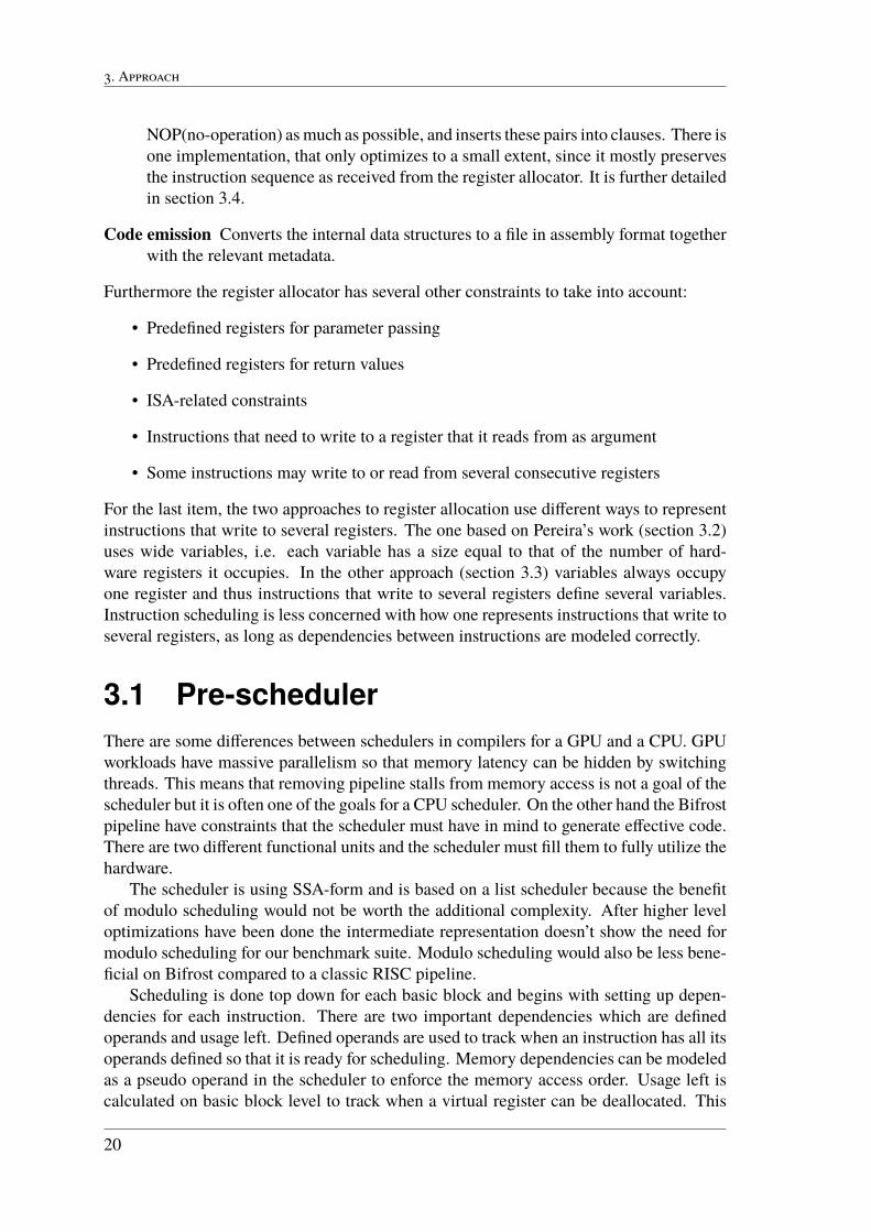
before0: a←mul1: b←div2: c←add a, b3: d ←sub

before in clause0-FMA: mul0-ADD: nop

1-FMA: div1-ADD: nop

2-FMA: nop2-ADD: add

3-FMA: nop3-ADD: sub

after0: b←div1: d ←sub2: a←mul3: c←add a, b

after in clause0-FMA: div0-ADD: sub

1-FMA: mul1-ADD: add

Figure 3.1: Example of scheduling

In this fictional example mul and div can only be executed in FMA unit while add andsub can only be executed in the ADD unit. For the figures in clauses the instructions areput in instruction pairs with the format "x-unit" where x is the pair index and unit, whichfunctional unit. A constraint in this example is that the result of a div is not available in thesame instruction pair which would make scheduling mul first sub-optimal. The downsidewith the scheduling is that d can’t be in the same register as a and b which may increaseregister pressure.

3.1.1 ModelThe scheduler uses a model of the hardware to be able to generate efficient code. The modelkeeps track of how long the clauses are, if an operand can be read as a bypass and otherconstraints. Because of the constraints the model is necessary for efficient code generation.Without a model the scheduled instructions may not work in the pipeline directly and sub-optimal fixes may be necessary. Because of the two distinct arithmetic functional units themodel keeps track of which unit that is available to fill both units with useful instructions.

3.1.2 Heuristics (priority function)Two important considerations for the scheduler are to fill the functional units and minimizeregister pressure. Filling functional units would benefit from having many instructionsready so that the probability of finding one that fits the pipeline is high. The problem ofkeeping many instructions ready for scheduling is that it often increases register pressure.This problem is solved by focusing on filling functional units when the register pressure islow and try to lower register pressure when register pressure is high. Some heuristics forlowering register pressure are the following:

• Prioritize instructions that kill live variables.

21

3. Approach

• Prioritize arithmetic instructions over memory load.

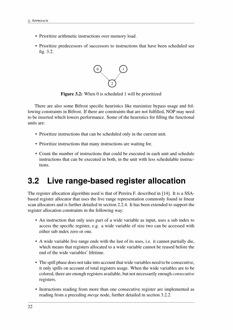
• Prioritize predecessors of successors to instructions that have been scheduled seefig. 3.2.

0 1

2

Figure 3.2: When 0 is scheduled 1 will be prioritized

There are also some Bifrost specific heuristics like maximize bypass usage and fol-lowing constraints in Bifrost. If there are constraints that are not fulfilled, NOP may needto be inserted which lowers performance. Some of the heuristics for filling the functionalunits are:

• Prioritize instructions that can be scheduled only in the current unit.

• Prioritize instructions that many instructions are waiting for.

• Count the number of instructions that could be executed in each unit and scheduleinstructions that can be executed in both, in the unit with less schedulable instruc-tions.

3.2 Live range-based register allocationThe register allocation algorithm used is that of Pereira F. described in [14]. It is a SSA-based register allocator that uses the live range representation commonly found in linearscan allocators and is further detailed in section 2.2.4. It has been extended to support theregister allocation constraints in the following way:

• An instruction that only uses part of a wide variable as input, uses a sub index toaccess the specific register, e.g. a wide variable of size two can be accessed witheither sub index zero or one.

• A wide variable live range ends with the last of its uses, i.e. it cannot partially die,which means that registers allocated to a wide variable cannot be reused before theend of the wide variables’ lifetime.

• The spill phase does not take into account that wide variables need to be consecutive,it only spills on account of total registers usage. When the wide variables are to becolored, there are enough registers available, but not necessarily enough consecutiveregisters.

• Instructions reading from more than one consecutive register are implemented asreading from a preceding merge node, further detailed in section 3.2.2

22

3.2 Live range-based register allocation

bb00: a〈rx〉 ← de f<1>1: b〈rx+1〉 ← de f<1>

bb10: ← a〈rx〉

rx → ry, rx+1 → rz1: c〈rx ,rx+1〉 ← de f<2>2: ← c[0]3: ← a4: ← c[1]

bb21: ← b

Figure 3.3: (a) Partially colored program with a shuffle instruction

3.2.1 Shuffle insertionIn order to handle the constraints placed on a register allocator as listed in chapter 3, shufflecode is inserted before the instruction to free the required registers (essentially a registerfile permutation). Mohr et al. [13] use a shuffle instruction to implement φ-functions andthe same concept can be reused here. An instruction that shuffles registers is defined asra → rx, rb → ry which copies the contents of register ra to rx and rb to ry. It may alsoinclude swaps rx ↔ ry and circular dependencies rx → ry, ry → rz, rz → rx . Whilst Mohret al. implements a shuffle instruction as a register file permutation hardware instruction,it usually needs to be implemented as several move or swap instructions in a similar wayto φ-deconstruction. If the hardware does not support swap instructions, a swap can beimplemented in the classical way with three XOR instructions. From here on it will beassumed that the more moves a shuffle instruction contains, the more expensive it will bein terms of computation cost and furthermore, swaps are more expensive than moves.

An issue with inserting shuffle code to handle the register allocation constraints isthat the register values need to be reshuffled in order to preserve program correctness.To illustrate this, and example program which has been partially colored can be seen infig. 3.3. The notation a〈rx〉 is used to signify that a variable a has been allocated to rx. Thisexample showcases the implementation regarding wide variables but the same techniquesare used for the rest of the constraints.

The register allocator has assigned register rx to the variable a and rx+1 to b. Whenit arrived at the definition of c in basic block 1, no two consecutive registers were free tohold c, so rx and rx+1 were freed by moving their contents to ry and rz, which are free forthe lifetime of c. In order for the uses of a and b in basic block 2 to use the correct values,the contents of rx and rx+1 need to be shuffled from ry and rz before those instructions areexecuted but only if the original shuffle has been encountered during execution. Two ap-proaches to ensuring that all registers get the correct values and that reshuffles are insertedappropriately are:

1. Reshuffle directly after the instruction

2. Reshuffle right before entering the dominance frontier of c ← de f<2>, i.e. the

23

3. Approach

bb00: a〈rx〉 ← de f<1>1: b〈rx+1〉 ← de f<1>

bb10: ← a〈rx〉

rx → ry, rx+1 → rz1: c〈rx ,rx+1〉 ← de f<2>rx ↔ ry, rx+1 ↔ rz2: ← c〈ry〉

3: ← c〈rz〉

4: ← a〈rx〉

bb21: ← b〈rx+1〉

(a)

bb00: a〈rx〉 ← de f<1>1: b〈rx+1〉 ← de f<1>

bb10: ← a〈rx〉

rx → ry, rx+1 → rz1: c〈rx ,rx+1〉 ← de f<2>2: ← c〈rx〉

3: ← c〈rx+1〉

4: ← a〈ry〉

rx → ry, rx+1 → rz

bb21: ← b〈rx+1〉

(b)

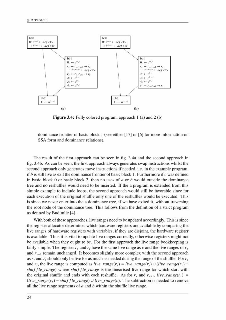
Figure 3.4: Fully colored program, approach 1 (a) and 2 (b)

dominance frontier of basic block 1 (see either [17] or [6] for more information onSSA form and dominance relations).

The result of the first approach can be seen in fig. 3.4a and the second approach infig. 3.4b. As can be seen, the first approach always generates swap instructions whilst thesecond approach only generates move instructions if needed, i.e. in the example program,if b is still live as exit the dominance frontier of basic block 1. Furthermore if c was definedin basic block 0 or basic block 2, then no uses of a or b would outside the dominancetree and no reshuffles would need to be inserted. If the a program is extended from thissimple example to include loops, the second approach would still be favorable since foreach execution of the original shuffle only one of the reshuffles would be executed. Thisis since we never enter into the a dominance tree, if we have exited it, without traversingthe root node of the dominance tree. This follows from the definition of a strict programas defined by Budimlic [4].

With both of these approaches, live ranges need to be updated accordingly. This is sincethe register allocator determines which hardware registers are available by comparing thelive ranges of hardware registers with variables, if they are disjoint, the hardware registeris available. Thus it is vital to update live ranges correctly, otherwise registers might notbe available when they ought to be. For the first approach the live range bookkeeping isfairly simple. The register ry and rz have the same live range as c and the live ranges of rxand rx+1 remain unchanged. It becomes slightly more complex with the second approachas ry and rz should only be live for as much as needed during the range of the shuffle. For ryand rz, the live range is computed as live_range(ry) = live_range(ry) ∪ (live_range(rx) ∩shu f f le_range) where shu f f le_range is the linearised live range for which start withthe original shuffle and ends with each reshuffle. As for rx and rx+1, live_range(rx) =(live_range(rx) − shu f f le_range) ∪ live_range(c). The subtraction is needed to removeall the live range segments of a and b within the shuffle live range.

24

3.3 Coupled register allocator

3.2.2 Wide variables as argumentsA merge node takes several variables as arguments and produces as variable of a size equalto the sum of the sizes of the arguments like, w ← merge<2> a, b. Thus a merge with twoarguments, both with a size of one, will produce a variable of size two. When the registerallocator reaches a merge instruction, it is treated similarly to any instruction that writes toseveral registers. In the case of a merge though, shuffles are only inserted if the argumentsof the merge do not match up to the assigned registers. For example, a merge takes fourarguments of size one that have been assigned to hardware registers 4, 5, 16 and 7. If theregister allocator assigns 4, 5, 6 and 7 to this merge node, then only a r16 ↔ r7 needs toinserted.

When coloring any variable, a preference list listing all possible hardware registersordered from most preferable to least preferable for this instruction is created. The purposeof this list in Pereira’s compiler [14] is to allow opportunities for φ register coalescing,i.e. choosing a register for the φ node that matches one or several of its arguments. Thispreference list can also be used to reduce the number of instructions generated by themerge.

When the preference list for an instruction i is generated, a check is done if any mergeinstructions read from i. If i is the first argument to this merge (i.e. if this is the firsttime this merge is visited as a use during preference list generation), then a bias register isreserved for this merge. The next time this merge is visited as a use of an instruction, theregister allocator tries to allocate a register, using the bias, such that the merge will resultin as few instructions as possible when it is colored.

3.3 Coupled register allocatorThis approach scalarizes all nodes in the internal representation. This means that loadsthat fetch to more than one register will get multiple virtual registers assigned to it. Storesthat store more than one register need to keep track of all the virtual registers they storeand their internal order.

Another difference of this approach is that it’s tightly coupled with the scheduler. Metadata from the scheduler is used to keep track of lifetimes instead of calculating live ranges.This means that this approach can be used for scheduling and allocation in unison. Thereare however some practical benefits of doing scheduling and register allocation sequen-tially. Some benefits is of doing it sequentially are that the scheduler can be used with thewide virtual registers approach. It is also a bit simpler to implement and debug the codewhen they are separated. Some parts of the text in section 3.3 are specific for when theallocator is run after the scheduler, modifications needed for running those two simultane-ously will be described in section 5.2.

3.3.1 SpillingWhen instructions are scheduled an interference graph is constructed if there are morelive variables than registers. This graph is the same as the graph in Chaitin’s[5] graphcoloring algorithm but is only constructed when register pressure is too high. The spilling

25

3. Approach

implementation also keeps track of intervals that needs spilling. This makes it possiblefor uses of a spilled variable to use the same reload if it’s outside a high register pressureinterval. Registers are spilled as 32 bit scalars but it’s possible to schedule spills to leveragewide memory instructions.

3.3.2 ColoringAn important feature of the coloring algorithm is the ability to support data that must bein adjacent registers. If virtual registers can’t be allocated to adjacent physical registersdirectly this pass will insert shuffles to correct it. The algorithm colors basic blocks inreverse post order and goes top to bottom within a basic block.

The current physical register a virtual register occupies will be called effective regis-ter. Every basic block has a data structure that maps every virtual register to its effectiveregister which enables shuffling around physical register effectively. If a virtual registeris live outside of a shuffles dominance tree the register must be shuffled back to ensurecorrectness. With the effective register system, back-shuffles can be inserted as a shufflefrom a virtual register to a physical register.φ-functions are deconstructed in the coloring phase by inserting a shuffle from the ar-

gument variable to φ-function’s physical register. If the φ-function does not have a physicalregister it will be assigned the same as one of its operands physical register. If the effectiveregister is the same as the destination of a shuffle the shuffle will simply be ignored. Whenthe effective register is different from the physical register moves or swaps needs to beinserted depending on if the physical destination is holding a live variable.

One property of reverse post order is that all predecessors excluding loops are coloredbefore the current basic block. This means that all operands from other basic blocks thatare not used in a φ-function will already have a color. Because of this property, the effectiveregister can be propagated by setting the same effective register in the successors wherethe correspondent variable is live.

Look aheadTo minimize unnecessary shuffles the coloring algorithm will check if the a variable hasa use with constraints. If a use is a wide store the algorithm will try to allocate a registerthat have as many free adjacent registers as the store is wide. The algorithm will also lookif a φ-function uses the variable and would preferably chose the same physical register toavoid shuffling.

3.4 Post schedulingThe Bifrost architecture expects assembly code in the form of clauses and instruction pairs.The task of this stage is to schedule instructions in the FMA or ADD unit and create clauseswith these scheduled instruction pairs. Each basic block is divided into several clauses anda clauses never contains instructions from two different basic blocks.

Barely any optimizations are done in this stage, it is assumed this is done in the sched-uler before register allocation. This stage also handles the various constraints of Bifrost

26

3.4 Post scheduling

instruction encoding, such as which instructions need to be passed constants through reg-isters and which can use them directly as arguments etc. It tries to pack the instructionsinto as few pairs as possible and rearranging of instructions is only done within a pair,e.g. if an instruction is scheduled in the ADD unit, and the following instruction may beexecuted in the FMA unit, provided it is not dependent on the result of the ADD, it isscheduled in the FMA unit.

27

3. Approach

28

Chapter 4Results

The test suite consists of 228 shaders that our back-end can compile and the generatedcode produce correct output. In order to be displayed, the tests have been grouped ac-cording several categories to differentiate how the back-end performs for different typesof shaders. Firstly, they may be grouped according to size (number of instructions directlyafter instruction selection), the size limits for each group can be seen in table 4.1. Fur-thermore, the test cases are also be divided into shaders that include 16 bit computationsand those that only perform 32 bit computations. Also, they may be divided into types ofshader: fragment shader, compute shader and vertex shader, which correspond to shadersfor different parts of the graphics pipeline.

The following metrics are used for the evaluation of the back-end:

Executed instruction pairs Gives a rough estimate how how many cycles that the shaderruns for

Number of instructions Statically counted number of instructions

Number of clauses Statically counted number of clauses

Table 4.1: Limits for size categories, number of instructions afterinstruction selection

category limits (number of instructions)very small < 10small 10 - 100medium 100 - 160large 160 - 270very large > 270

29

4. Results

The reason why not, for example, the run time of the shader program was used as metricis that it was not deemed worthwhile to start optimizing for execution time from the start.Instead focus was on reducing the number of executed instruction pairs, and the plan was tostart comparing execution time when the difference in the number of executed instructionpairs was low enough. Unfortunately, due to time constraints, this was never done.

Whilst the number of clauses and the number of instructions do not give a exact mea-sure of performance, they can still be used to compare the effectiveness of code generationcompared to the reference compiler which is a compiler developed at ARM. Some metricsmay be presented as normalized with regards to the reference compiler, e.g. if the codegenerated by our back-end results in 30 executed instruction pairs and the same shadercompiled by the reference compiler results in 20 executed instruction pairs, then the dis-played value would be 30

20 = 1.5.

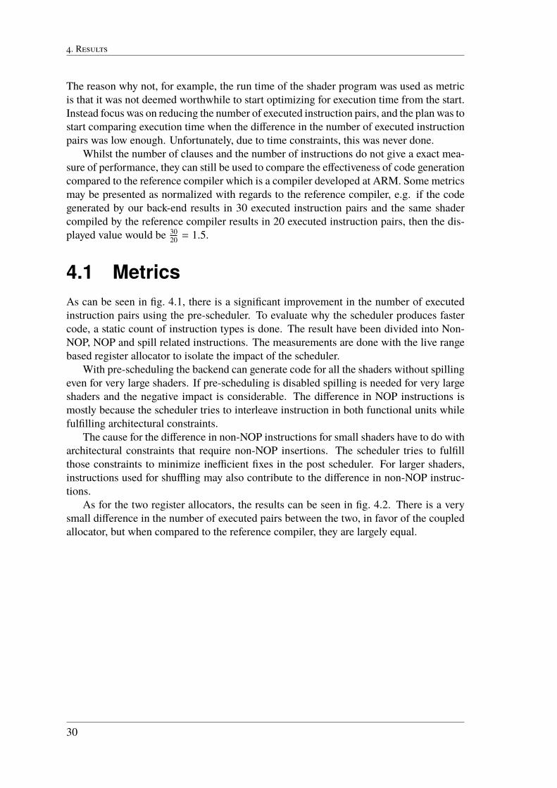
4.1 MetricsAs can be seen in fig. 4.1, there is a significant improvement in the number of executedinstruction pairs using the pre-scheduler. To evaluate why the scheduler produces fastercode, a static count of instruction types is done. The result have been divided into Non-NOP, NOP and spill related instructions. The measurements are done with the live rangebased register allocator to isolate the impact of the scheduler.

With pre-scheduling the backend can generate code for all the shaders without spillingeven for very large shaders. If pre-scheduling is disabled spilling is needed for very largeshaders and the negative impact is considerable. The difference in NOP instructions ismostly because the scheduler tries to interleave instruction in both functional units whilefulfilling architectural constraints.

The cause for the difference in non-NOP instructions for small shaders have to do witharchitectural constraints that require non-NOP insertions. The scheduler tries to fulfillthose constraints to minimize inefficient fixes in the post scheduler. For larger shaders,instructions used for shuffling may also contribute to the difference in non-NOP instruc-tions.

As for the two register allocators, the results can be seen in fig. 4.2. There is a verysmall difference in the number of executed pairs between the two, in favor of the coupledallocator, but when compared to the reference compiler, they are largely equal.

30

4.1 Metrics

16 32 comp frag large medium small vert vlarge vsmall0.0

0.2

0.4

0.6

0.8

1.0

1.2

1.4

1.6

Norm

aliz

ed t

o p

resc

hed

Static instruction count

Non-NOP NOP Spill LOAD/STORE Without presched With presched

Figure 4.1: Static instruction count with and without pre-scheduler

16 32 comp frag large medium small vert vlarge vsmall0.0

0.2

0.4

0.6

0.8

1.0

1.2

1.4

1.6

Norm

aliz

ed t

o r

efe

rence

Number of executed instruction pairs

Coupled register allocator Live range register allocator

Figure 4.2: The number of executed instruction pairs for eachregister allocator with pre-scheduling enabled for both allocators

31

4. Results

32

Chapter 5Discussion

In general, the two approaches to register allocation are equal but as can be seen in fig. 4.2,there are slight differences. These can be seen more clearly in Appendix B and are partlydue to the coupled allocator producing less shuffle code. It has implemented more op-timizations toward register coalescing with φ-functions (i.e. bias for the coloring of theφ) which the live range allocator only implements for wide variables. In the latter, theregisters allocated to a wide variable are allocated for the entire live range of the widevariable, whilst in the former the registers which are no longer needed, may be used byother instructions. This may increase register pressure which in turn might create the needfor more shuffle code. The difference is not due to one of the allocators spilling though,since with the pre-scheduler, neither of the two do any spilling.

The graph in Appendix A shows that the difference in performance between our back-end and the reference in the number of executed instruction pairs is related to the differencein the number of instructions (statically counted) generated by the two compilers, which isconfirmed when examining the differences in the generated code as well. Essentially, theinstruction selection of our back-end does not measure up to that of the reference compiler.The difference in the number of executed instruction pairs is not merely the product ofinstruction selection differences thoughs since, as can be seen in Appendix A, the numberof NOPs in the generated in the code differs as well. This is a product of the schedulingalgorithms (both pre- and post-scheduling).

5.1 Coupled register allocatorThe coupled registers allocator was designed with the following requirements in mind:

• There are wide memory instructions that require adjacent registers.

• There are hardware benefits from using bypass registers within a clause.

33

5. Discussion

• Other constraints in the hardware that need to be addressed.

Splitting a wide memory instructions into multiple variables can lower the registerpressure. Uses of parts in a wide memory load may be far apart and it’s unnecessary tokeep a part that won’t be used live, see fig. 5.1. One downside of splitting variables is thatit increases number of variables and may affect compile time negatively.

1: a← de f<2>2: ← a[0]...x: ← a[1]

Figure 5.1: a[0] don’t have to be live after 2

Because of those wide memory instructions it’s sometimes necessary to shuffle reg-isters so that the required registers can be adjacent. The "effective register" approach isdesigned to simplify shuffling. With it, shuffles are defined as moving a variable to aphysical register. This enables the compiler to shuffle registers without doing complexcalculations when a variable is shuffled multiple times. It is also a causal system that canbe done without knowing the future which is a prerequisite for doing register allocationwith instruction scheduling.

The choice of letting the scheduler set up information of when a variable can be killedis also done so that the register allocation can be done simultaneously. Much focus hasbeen put on the ability to allocate register with instruction scheduling to build clauses anduse bypass registers. The register allocator can be seen a just-in-time linear scan allocatorwith support for wide memory instructions.

Spilling can be avoided in our test suite with the pre-scheduler so this approach didn’tput much effort in optimizing spilling. It can output correct code for all the tests that spillwithout the pre-scheduler but performance may suffer.

5.2 Unified Scheduling and Register Allo-cation

Scheduling and Register allocation can be done in unison with the coupled register alloca-tor. The post scheduler is also an integrated part of this approach. When an instruction isscheduled, a register will be allocated and the instruction will be inserted in a clause im-mediately. There are three parts that are executed every time an instruction is selected forinsertion. The scheduler will first choose a instruction based on a modified heuristic withregister continuity in mind. After that the allocator will assign registers and if shuffling isneeded the shuffled code will be inserted before the instruction. A post pass will then bedone after every insertion to make sure that all constraints are fulfilled. The post pass willcreate instruction pairs and clauses directly so that the model will mirror the current stateaccurately. The spilling algorithm for register allocation after scheduling won’t work nowbut possible solutions will be described later.

Implementation of this unified code generator is unfortunately not mature enough toproduce efficient code yet. It can run all of the shaders used in our benchmark suite but

34

5.2 Unified Scheduling and Register Allocation

the instruction pairs count is around 10% worse. There are however lessons learned aboutthe advantages and disadvantages with a combined code generator.

After some experimentation with this unified approach it was noted that the increasedfreedom and model precision was too much for our limited time frame. The heuristicsbecame quite complex and conflicts in the heuristics sometimes produced code with lowerquality. The additional freedom has the potential to produce better code but the cost indeveloping heuristics and compilation time may be high.

Wide memory instructionsOne disadvantage of doing register allocation and instruction scheduling simultaneously isthat the register allocator cannot look ahead to see how long a variable is alive. In fig. 5.2at cycle 1 a will be allocated to r0 and r1 will be reserved for b because of the store in cyclez. Without knowing when c will die the register allocator won’t allocate c to r1 which maybe the optimal solution. The advantage on the other hand is that the scheduler can activelyoptimize the problem by killing problematic variables. The register allocator can also seeif a variable is ready to be killed by looking if it’s last use is ready for scheduling.

1: a← de f<1>2: c ← de f<1>...x: ← cy: b← de f<1>z: ← a, b

Figure 5.2: c can be allocated to b’s reserved register

SpillingSpilling benefits from knowing interference between variables to do a relatively optimalspill. It is impossible to know how the interference for instructions that haven’t been sched-uled yet, which may be a problem. It may also be better to insert spill in a position thatalready has been scheduled. If that is done the spill will probably be less optimal com-pared to scheduling the spill in a post scheduler. The benefits may include that reloadinga spill can be scheduled more optimally and that spill may be avoided with use of bypassregisters. The simple way is to spill a variable directly when the register pressure gets toohigh. But that approach may spill variables inside a loop which is sub-optimal. It’s possi-ble to make better spills in other places of the code but that scheme may be quite complexbecause of different constrains.

HeuristicsWhen scheduling is done in unison with the register allocation the heuristic can be mademore optimally and more complex. Because clauses are created directly, the model is nolonger an approximation so the heuristic can be much more precise. This will for examplemake it possible for the scheduler to optimize for long clauses. As discussed before the

35

5. Discussion

schedulers heuristic may now consider register allocation problems and the allocators lookahead may look into the scheduler.

More efficient code could be generated if the scheduler scheduled a few instructions ata time because some constraints that depend on following instructions could be optimized.This may increase the compilation time depending on how many instruction in the futurethat will be evaluated.

ConclusionsDoing Register Allocation and Instruction Scheduling in unison gives a lot of freedom andand a better model. The downside is the increased complexity and problematic spilling.The improved heuristics and spilling haven’t been implemented yet and are candidates forfuture work.

5.3 Live range based register allocatorAs mentioned above, there are a number of points to improve on the live range basedregister allocator,

• Faster compilation time

• Better optimizations for shuffle code reduction (probably bug)

• φ bias for coloring

The first point could be addressed by improving how the instructions access register argu-ments that may have been shuffled as described by section 3.2. The current implementationis based on the live ranges used to represent instruction live ranges, and when the argu-ments of an instruction are to be hardened into their hardware register equivalents, a lookup is done to find if an instruction is within the region defined by a shuffle. These re-gions may be layered, which further increases the time it takes to find the correct register.Furthermore, the creation of the preference list used for register coalescing is relativelyunoptimized as well.

The general evaluation for this allocator is that, at least for the shaders comprising thetest suite, it is not necessary for the register allocator to be complex as long as the pre-scheduling lowers the register pressure enough. As for future work, something interestingto investigate would be allocating register to variables in decreasing size, ensuring thatwide variables are always allocated to wide registers and less shuffle code would be needed.

5.4 Post schedulingIn the post-scheduler, an opportunity for optimization is with regards to clause length. Asstated in section 3.4, the post-scheduler assumes that the instructions are already sched-uled well and merely attempts to pack into as few instruction pairs as possible. The issuewith this is that there are some instructions in the Bifrost ISA that need to be in the lastinstruction pair of the clause and others which result is not available before the next clause

36

5.4 Post scheduling

executes, i.e. their result cannot be used before the clause has finished executing. At themoment, the post scheduler handles these types of instructions in the same way: they both,when scheduled, force the scheduler to create a new clause in which the rest of the instruc-tions may be inserted to. For the instructions that do not need to end a clause but forwhich the result is not available in the current clause, unrelated instructions may be in-serted to increase the length of the clause. This would require dependency analysis, whichthe post-scheduler does not have.

The post-scheduler might also benefit from rearranging instructions as well, so as tonot depend on scheduling done by the pre-scheduler, since it cannot schedule instructionsintroduced by the register allocator. For the shaders used in the test suite, no spilling wasdone but some shuffle code was introduced so the register allocator does not introduce largeamounts of code and whether or not it would result in large gains to include instructionsrearranging in the post-scheduler is hard to determine. In the general case, especially ifthe register allocator inserts much spill and shuffle-code, instruction rearranging in thepost-scheduler would definitely be beneficial.

37

5. Discussion

38

Chapter 6Conclusions

In this thesis multiple approaches have been presented for back-end code generation andtheir respective pros and cons evaluated. We found that a pre-scheduler can lower theregister pressure considerably which makes a major impact on part of our tests. Further-more the pre-scheduler can also increase the utilisation level of the hardware by executinginstruction in a more optimal way.

There was no major difference in the quality of the generated code between the tworegister allocation algorithms for our test suite. Generated register shuffling for both ap-proaches was minimal and was not responsible for any significant portion of the differencein executed instruction pairs.

Instruction selection and higher level optimisations made a major impact on the resultfor some of our tests but does not explain all of the differences in executed instructions.The rest of the differences in executed instructions are probably because of suboptimalscheduling in the pre- and post-scheduler.

6.1 Future workImprovements can be done for all parts of the back-end presented in this thesis. There isa lot of room for improvement in the pre-scheduler heuristics. Example of improvementsinclude a better balance between register pressure and number of ready instruction to in-crease utilization of the hardware. The register allocators can benefit from a better coloringalgorithm for more complex shaders to avoid unnecessary shuffling and phi deconstructinstructions. Spilling could also be improved as our benchmark only covers the correct-ness and not the efficiency of spilling. The post scheduler can be improved by allowing itto schedule a basic block instead of only an instruction pair.

It would also be interesting to fully implement combined scheduling and register allo-cation for comparison. There are a lot of architecture-specific improvements to be madein both pre- and post-scheduler. Those improvements may include scheduling memory

39

6. Conclusions

access, fulfilling constraints and minimize the number of clauses. Instruction selectioncould also be improved with more advanced optimizations.

40

Bibliography

[1] L. A. Belady. A study of replacement algorithms for a virtual-storage computer. IBMSyst. J., 5(2):78–101, June 1966.

[2] David G. Bradlee, Susan J. Eggers, and Robert R. Henry. Integrating register allo-cation and instruction scheduling for RISCs. SIGPLAN Not., 26(4):122–131, April1991.

[3] Preston Briggs, Keith D. Cooper, and Linda Torczon. Improvements to graph col-oring register allocation. ACM Trans. Program. Lang. Syst., 16(3):428–455, May1994.

[4] Zoran Budimlic, Keith D. Cooper, Timothy J. Harvey, Ken Kennedy, Timothy S.Oberg, and Steven W. Reeves. Fast copy coalescing and live-range identification.SIGPLAN Not., 37(5):25–32, May 2002.

[5] G. J. Chaitin. Register allocation & spilling via graph coloring. SIGPLAN Not.,17(6):98–101, June 1982.

[6] Ron Cytron, Jeanne Ferrante, Barry K. Rosen, Mark N. Wegman, and F. KennethZadeck. Efficiently computing static single assignment form and the control depen-dence graph. ACM Trans. Program. Lang. Syst., 13(4):451–490, October 1991.

[7] Lal George and Andrew W. Appel. Iterated register coalescing. ACM Trans. Pro-gram. Lang. Syst., 18(3):300–324, May 1996.

[8] Philip B. Gibbons and Steven S. Muchnick. Efficient instruction scheduling for apipelined architecture. SIGPLAN Not., 21(7):11–16, July 1986.

[9] Sebastian Hack. Register Allocation for Programs in SSA Form. PhD thesis, Univer-sität Karlsruhe, October 2007.

[10] Sebastian Hack, Daniel Grund, and Gerhard Goos. Register allocation for programsin SSA-form. In Proceedings of the 15th International Conference on CompilerConstruction, CC’06, pages 247–262, Berlin, Heidelberg, 2006. Springer-Verlag.

41

BIBLIOGRAPHY

[11] Niklas Jonsson and Johan Ju. Evaluating existing code generation techniques for aGPU architecture. Report from EDAN70 project course at LTH, 2016.

[12] M. Lam. Software pipelining: An effective scheduling technique for VLIW ma-chines. SIGPLAN Not., 23(7):318–328, June 1988.

[13] Manuel Mohr, Artjom Grudnitsky, Tobias Modschiedler, Lars Bauer, SebastianHack, and Jörg Henkel. Hardware Acceleration for Programs in SSA form. In Pro-ceedings of the 2013 International Conference on Compilers, Architectures and Syn-thesis for Embedded Systems, CASES ’13, pages 14:1–14:10, Piscataway, NJ, USA,2013. IEEE Press.

[14] Fernando Magno Quintão Pereira. The design and implementation of a SSA-basedregister allocator. Technical report, UCLA - University of California, 2007.

[15] Fernando Magno Quintão Pereira and Jens Palsberg. Register allocation via color-ing of chordal graphs. In Proceedings of the Third Asian Conference on Program-ming Languages and Systems, APLAS’05, pages 315–329, Berlin, Heidelberg, 2005.Springer-Verlag.

[16] Massimiliano Poletto and Vivek Sarkar. Linear scan register allocation. ACM Trans.Program. Lang. Syst., 21(5):895–913, September 1999.

[17] Jonas Skeppstedt. An Introduction to the Theory of Optimizing Compilers. SkeppbergAB, 2016. Extended 1 st. Edition, with performance measurements on POWER.

[18] Sid Touati and Benoit Dupont de Dinechin. Advanced Backend Code Optimization.ISTE Ltd and John Wiley & Sons, Inc., 2014.

[19] Alan Tsai. Bifrost - the GPU architecture for next five billion. ARM Tech ForumTaipei [Accessed: 2016-11-28], July 2016.

[20] Christian Wimmer and Michael Franz. Linear scan register allocation on SSA form.In Proceedings of the 8th Annual IEEE/ACM International Symposium on Code Gen-eration and Optimization, CGO ’10, pages 170–179, New York, NY, USA, 2010.ACM.

42

Appendices

43

Appendix ATest suite listing 1

This appendix lists all test cases with the number of executed instruction pairs, number ofinstructions excluding NOP and number of clauses for each shader, with and without thepre-scheduler for the live range register allocator. They are divided into the 16 and 32 bitcategories as explained in chapter 4 for readability.

45

A. Test suite listing 1

0.6

0.8 1

1.2

1.4

1.6

1.8 2

002_00

007_00

009_00

011_00

013_00

015_00

027_00

029_00

031_00

033_00

035_00

037_00

039_00

041_00

043_00

045_00

047_00

049_00

051_00

053_00

055_00

057_00

059_00

061_00

063_00

065_00

067_00

069_00

071_00

073_00

075_00

087_00

089_00

091_00

093_00

095_00

107_00

109_00

111_00

113_00

115_00

117_00

119_00

121_00

123_00

125_00

127_00

129_00

131_00

133_00

135_00

137_00

139_00

141_00

143_00

145_00

instruction pairs / no-NOP instructions/ clauses normalized to reference

Instruction pairsE

xcluding N

OP

Clauses

0.6

0.8 1

1.2

1.4

1.6

1.8 2

147_00

149_00

151_00

153_00

155_00

157_00

159_00

161_00

163_00

165_00

167_00

169_00

171_00

173_00

175_00

177_00

179_00

181_00

183_00

185_00

187_00

189_00

191_00

193_00

195_00

197_00

199_00

201_00

203_00

205_00

207_00

209_00

211_00

213_00

215_00

217_00

219_00

221_00

225_00

229_00

235_00

239_00

241_00

245_00

247_00

248_00

250_00

259_00

262_00

263_00

266_00

268_00

274_00

276_00

278_00

instruction pairs / no-NOP instructions/ clauses normalized to reference

Instruction pairsE

xcluding N

OP

Clauses

Figure A.1: With 16bit instructions

46

0.6

0.8 1

1.2

1.4

1.6

1.8 2

001_00

006_00

008_00

010_00

012_00

014_00

016_00

017_00

019_00

020_00

021_00

022_00

023_00

024_00

025_00

026_00

028_00

030_00

032_00

034_00

036_00

038_00

040_00

042_00

044_00

066_00

068_00

070_00

072_00

074_00

076_00

078_00

082_00

084_00

086_00

088_00

090_00

092_00

094_00

096_00

098_00

102_00

104_00

106_00

108_00

110_00

112_00

114_00

116_00

118_00

120_00

122_00

124_00

instruction pairs / no-NOP instructions/ clauses normalized to reference

Instruction pairsE

xcluding N

OP

Clauses

0.6

0.8 1

1.2

1.4

1.6

1.8 2

126_00128_00130_00132_00134_00136_00138_00140_00142_00144_00146_00148_00150_00152_00154_00156_00158_00160_00162_00164_00166_00168_00170_00172_00174_00176_00178_00180_00182_00184_00186_00188_00190_00192_00194_00196_00198_00200_00202_00204_00206_00208_00210_00212_00214_00216_00218_00220_00222_00224_00226_00228_00230_00232_00234_00240_00242_00243_00244_00249_00257_00258_00261_00267_00

instruction pairs / no-NOP instructions/ clauses normalized to reference

Instruction pairsE

xcluding N

OP

Clauses

Figure A.2: Only 32bit instructions

47

A. Test suite listing 1

48

Appendix BTest suite listing 2

This appendix lists all test cases with the number of executed instruction pairs for the liverange allocator, live range allocator without pre-scheduler and coupled allocator

49

B. Test suite listing 2

0.6

0.8 1

1.2

1.4

1.6

1.8 2

002_00

007_00

009_00

011_00

013_00

015_00

027_00

029_00

031_00

033_00

035_00

037_00

039_00

041_00

043_00

045_00

047_00

049_00

051_00

053_00

055_00

057_00

059_00

061_00

063_00

065_00

067_00

069_00

071_00

073_00

075_00

087_00

089_00

091_00

093_00

095_00

107_00

109_00

111_00

113_00

115_00

117_00

119_00

121_00

123_00

125_00

127_00

129_00

131_00

133_00

135_00

137_00

139_00

141_00

143_00

145_00

executed instruction pairs normalized to reference

Live range allocator

Withou

t preschedC

oupled allocator

0.6

0.8 1

1.2

1.4

1.6

1.8 2

147_00

149_00

151_00

153_00

155_00

157_00

159_00

161_00

163_00

165_00

167_00

169_00

171_00

173_00

175_00

177_00

179_00

181_00

183_00

185_00

187_00

189_00

191_00

193_00

195_00

197_00

199_00

201_00

203_00

205_00

207_00

209_00

211_00

213_00

215_00

217_00

219_00

221_00

225_00

229_00

235_00

239_00

241_00

245_00

247_00

248_00

250_00

259_00

262_00

263_00

266_00

268_00

274_00

276_00

278_00

executed instruction pairs normalized to reference

Live range allocator

Withou

t preschedC

oupled allocator

Figure B.1: With 16bit instructions

50

0.6

0.8 1

1.2

1.4

1.6

1.8 2

001_00

006_00

008_00

010_00

012_00

014_00

016_00

017_00

019_00

020_00

021_00

022_00

023_00

024_00

025_00

026_00

028_00

030_00

032_00

034_00

036_00

038_00

040_00

042_00

044_00

066_00

068_00

070_00

072_00

074_00

076_00

078_00

082_00

084_00

086_00

088_00

090_00

092_00

094_00

096_00

098_00

102_00

104_00

106_00

108_00

110_00

112_00

114_00

116_00

118_00

120_00

122_00

124_00

executed instruction pairs normalized to reference

Live range allocator

Withou

t preschedC

oupled allocator

0.6

0.8 1

1.2

1.4

1.6

1.8 2

126_00128_00130_00132_00134_00136_00138_00140_00142_00144_00146_00148_00150_00152_00154_00156_00158_00160_00162_00164_00166_00168_00170_00172_00174_00176_00178_00180_00182_00184_00186_00188_00190_00192_00194_00196_00198_00200_00202_00204_00206_00208_00210_00212_00214_00216_00218_00220_00222_00224_00226_00228_00230_00232_00234_00240_00242_00243_00244_00249_00257_00258_00261_00267_00

executed instruction pairs normalized to reference

Live range allocator

Withou

t preschedC

oupled allocator

Figure B.2: Only 32bit instructions

51

INSTITUTIONEN FÖR DATAVETENSKAP | LUNDS TEKNISKA HÖGSKOLA | PRESENTATIONSDAG 2017-06-02

EXAMENSARBETE Develop and prototype code generation techniques for a clause-based GPUSTUDENT Johan Ju, Niklas JonssonHANDLEDARE Jonas Skeppstedt (LTH), Markus Lavin (ARM), Dmitri Ivanov (ARM)EXAMINATOR Krzysztof Kuchcinski (LTH)

Kodgenerering for grafikprocessor

POPULARVETENSKAPLIG SAMMANFATTNING Johan Ju, Niklas Jonsson

Grafikprestandan spelar en allt större roll i dagens smartphones då den ofta bestämmerhur responsiv upplevelsen är av krävande applikationer. Detta arbete har utforskatkodgenereringstekniker för en modern grafikprocessor i syfte att förbättra prestandan.

Grafikprestanda blir en allt viktigare faktor iköpet av en mobiltelefon, dock begränsas förbät-tringmöjligheterna av batterikapaciteten och för-mågan att leda bort värme. Hårdvaruföretag pres-sas allt mer för att förbättra prestandan utanatt förkorta batteritiden och generera för mycketvärme. Ett sätt att uppnå detta är att flytta logikfrån hårdvara till mjukvaran. Ett exempel för attillustrera logik i hårdvaran kan vara att jämföragrafikprocessorn med muskler och mjukvaran medhjärnan. Att ha logik i hårdvaran innebär att jagkan tänka "flytta min hand" medan logik i mjuk-varan innebär att jag måste tänka "Flytta arm-bågen så många grader, vrid underarmen och böjhandleden etc.". Kodgenerering handlar om attgenerera instruktioner i hjärnan som styr armen.Detta arbete har undersökt kodgenerering för engrafikarkitektur av det senare laget vilket betyderatt mycket av logiken har flyttats till mjukvaran.Vi har implementerat traditionella och specialan-passade tekniker för kodgenerering och utvärderatdessa.

Kodgenerering kan framförallt delas upp i tvåsteg, instruktionsschemaläggning och registeral-lokering. Målet med instruktionsschemaläggningär att utnyttja beräkningsresurser i hårdvaran påett effektivt sätt. Man kan tänka sig att instruk-tionsschemaläggning är som om det fanns en kötill två automater. Om ena automaten endast taremot kort och den andra endast tar emot kontan-

ter så vill man att kön ska vara varannan medkontant och varannan med kort för att inte en au-tomat ska stå och vänta.Registerallokering innebär att placera den mest

använda datan i så kallade register (liten la-gringsplats med snabb access, tänk skrivbord) ochresterande i datorns minne (stor lagringsplats medlångsam access, tänk bibliotek). Då kan register-allokering jämföras med att planera sina besök tillbiblioteket så att de blir så få som möjligt ochlägga de mest använda böckerna på skrivbordetför att komma åt dem snabbt.Resultaten som vi kom fram till visar på att

det går att göra kodgenereringen mer än dubbeltså snabbt som en referens-kodgenerator. Dockså är koden inte alltid lika effektiv men vi trorpå att kodkvaliten kan förbättras genom att för-bättra schemaläggningen. Vi har även sett attschemaläggning kan ha betydlig påverkan på reg-isterallokeringen i båda riktningarna. Tradi-tionellt sätt så brukar instruktionsschemaläggningoch register allokering ske sekvensiellt men vi haräven undersökt ett sätt att göra det samtidigt un-der vissa förutsättningar vilket kan innebära attkoden som genererats blir bättre. Vi har även fun-nit att det kan vara en god ide att göra schemaläg-gning både före och efter registerallokeringen.