Determining Typical Ambient Noise Levels in the Presence of

Construction

Vahndi Minah

Abstract—Determining ambient noise levels in the presence of construction is a difficult and time consuming task, and the lack of

dedicated analysis and visualisation tools can lead to much disagreement between interested parties about typical ambient levels.

This paper presents an approach inspired by previous work on cluster-based analysis and visualisation of daily energy usage patterns,

and demonstrates substantial success in achieving the aim of establishing typical ambient noise levels, as well as raising further

questions about what typical truly means.

Index Terms—Environmental noise, construction noise, clustering, visualisation.

INTRODUCTION

It has become fairly standard practice for large construction projects in the UK,

such as CTRL [1], Crossrail [2], and Thames Tideway Tunnel [3], to provide

compensation for nearby businesses and residents who are predicted to be

adversely affected by construction works, even after the application of

mitigation using “Best Practicable Means”, as defined in Section 72 of the

Control of Pollution Act 1974 [4]. This compensation is typically noise and

vibration mitigation packages in the form of secondary glazing and / or

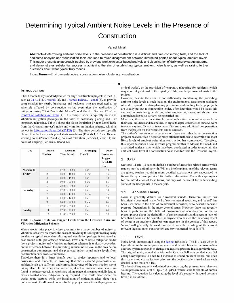
temporary rehousing. Table 1 shows the Noise Insulation Trigger Level Table

from the Crossrail project’s noise and vibration mitigation scheme, which is

set out in Information Paper D9 (IP D9) [5]. The time periods are typically

chosen to reflect site start-up and shut-down hours (Periods 1, 3, 6 and 8), core

working hours (Periods 2 and 7), hours of relaxation (Periods 4, 9 and 11) and

hours of sleeping (Periods 5, 10 and 12).

Day Period

Number

Relevant

Time Period

Averaging

Time T

Noise

Insulation

Trigger

Level dB

LAeq, T

Monday to

Friday

1 07:00 – 08:00 1 hr 70

2 08:00 – 18:00 10 hrs 75

3 18:00 – 19:00 1 hr 70

4 19:00 – 22:00 3 hrs 65

5 22:00 – 07:00 1 hr 55

Saturday 6 07:00 – 08:00 1 hr 70

7 08:00 – 13:00 10 hrs 75

8 13:00 – 14:00 1 hr 70

9 14:00 – 22:00 3 hrs 65

10 22:00 – 07:00 1 hr 55

Sunday 11 07:00 – 21:00 1 hr 65

12 21:00 – 07:00 1 hr 55

Table 1 - Noise Insulation Trigger Levels from the Crossrail Noise and

Vibration Mitigation Scheme

Where works take place in close proximity to a large number of noise- or vibration- sensitive receptors, the costs of providing this mitigation can quickly

escalate (a typical secondary glazing and ventilation package is estimated to

cost around £300 per affected window). Provision of noise mitigation under these projects' noise and vibration mitigation schemes is typically dependent

on the difference between the prevailing ambient noise level in the area before

construction commences, and the predicted and/or actual noise levels from construction once works commence.

Therefore there is a large benefit both to project sponsors and to local

businesses and residents, in ensuring that the measured pre-construction ambient levels are sufficient and correct, in advance of the construction works

taking place. In the worst case scenarios, if actual ambient noise levels are

found to be incorrect whilst works are taking place, this can potentially lead to extra uncosted noise mitigation being required. This could mean either the

works being stopped while the installation of mitigation takes place (at a

potential cost of millions of pounds for large projects on sites with programme-

critical works), or the provision of temporary rehousing for residents, which

may come at great cost to their quality of life, and large financial costs to the project.

However, despite the risks in not sufficiently ascertaining the prevailing

ambient noise levels at each location, the environmental assessment packages of work required to obtain planning permission and funding for large projects

are usually put out to competitive tender, often later than would be ideal; this

can lead to costs being cut during value engineering stages, and shorter, less comprehensive noise surveys being carried out.

Moreover, there is an incentive for local authorities, who are answerable to

their local residents and businesses, to argue that pre-construction surveys were in some way insufficient or inaccurate if it can secure additional compensation

from the project for their residents and businesses.

The author’s professional experience on these and other large construction projects has identified a need for more efficient methods to determine the most

likely levels of ambient noise after construction has commenced. Therefore,

this report describes a new software program written to address this need, and associated analysis tasks which have been conducted in order to ascertain the

ambient noise level at a construction noise monitor from the Crossrail Project.

1 DATA

Sections 1.1 and 1.2 section define a number of acoustics-related terms which

readers may be unfamiliar with. Whilst a brief explanation of the relevant terms

are given, readers requiring more detailed explanations are encouraged to

follow the hyperlinks provided for further information. The author apologises

for the introduction of these terms, but they will be useful for understanding

some of the later points in the analysis.

1.1 Acoustic Theory

Noise is generally defined as ‘unwanted sound’. Therefore ‘noise’ has historically been used in the field of environmental acoustics, and ‘sound’ has

been used more in the field of architectural acoustics, or to describe acoustic

pressure fluctuations in the more general sense. However there has recently been a push within the field of environmental acoustics to not be so

presumptuous about the desirability of environmental sound; a certain level of broadband noise can be desirable (as anyone who has felt the unnerving effect

of being in an anechoic chamber can attest to). In the context of this report,

‘noise’ will generally be used, consistent with the wording of the current relevant legislation on construction and environmental noise [6] [7].

1.1.1 Level

Noise levels are measured using the decibel (dB) scale. This is a scale which is

logarithmic in the sound pressure levels, and is used because the mammalian

auditory system responds to changes in acoustic pressure in a logarithmic way. The original scale, named after Alexander Graham Bell, sets out that a one Bel

change corresponds to a ten-fold increase in sound pressure levels, but since

this scale is too coarse for everyday use, the decibel scale is used where each decibel is one tenth of a Bel.

The level of any sound is calculated by comparing the pressure to a reference

sound pressure level of 0 dB (pref = 20 µPa.), which is the threshold of human hearing. The equation for calculating the level of a sound with sound pressure

level p is as follows:

L = 10 × log10

p

pref

1.1.2 Frequency

The frequency of sound is the rate at which pressure waves oscillate about the

standard atmospheric pressure, and is measured in Hertz (Hz). 1 Hz corresponds to an oscillation of one cycle per second. The frequency range of

human hearing is from approximately 20 Hz to 20 kHz for a young adult with

good hearing, although the upper range decreases markedly with age, as damage is done to the cochlea cells in the inner ear.

Frequency is loosely related to musical pitch. The mammalian auditory system

also responds to frequency in a logarithmic fashion. Plainly put, a doubling in the frequency of a sound corresponds to a one octave increase in the pitch. Pure

tones consist of a single frequency. Musical instruments typically have most of

their energy at the fundamental frequency and integer multiples of it, which is what gives them their specific timbre. Noise is generally ‘broadband’,

consisting of energy distributed across the audible spectrum.

1.1.3 Sound Propagation

The level of a sound decays with distance from the emitting source. The rate

of decay is dependent on the type of source generating the sound. Sound from an object acting as a point source, for example a small piece of machinery, is

attenuated at a rate of 6 dB per doubling of distance from the source. Sound

from an object acting as an infinite line source, for example a road with a steady stream of traffic, is attenuated at a rate of 3 dB per doubling of distance. In

reality, there are no infinite line sources; however, the 3 dB rate of attenuation

is a good approximation which is commonly used. Sound is also attenuated by objects between the source and receiver location

acting as noise barriers. When the barrier object partially obscures the line of sight from the source to the receiver, the sound is attenuated by approximately

5 dB. When the line of sight is completely blocked, the sound is attenuated by

approximately 10 dB. Up to 20 dB of attenuation can be achieved in theory; however, the material used for noise barriers on construction sites is typically

not of sufficient mass or adequacy of construction to prevent transmission of

sound through the barrier, so 10 dB of attenuation is a realistic upper limit when dealing with construction noise.

1.1.4 Rules of thumb

Some handy rules of thumb for thinking about sound are:

A 1 dB change corresponds to a just-noticeable difference in the level of

a pure tone.

A 3 dB change corresponds to a noticeable difference in the level of

broadband noise (broadband noise consists of sound across the frequency spectrum.

A 10 dB increase in sound pressure level corresponds to a subjective doubling in perceived loudness of the sound.

A 3 dB increase, i.e. a doubling of the acoustic energy in the sound, is

generally considered a significant increase and is used as the level at which environmental noise impacts are identified.

A 5 dB increase is sometimes used to trigger mitigation for construction noise, since the effect of a relatively short term increase in noise level is

considered lesser than a permanent change.

Adding two sounds with the same level produces a combined sound with a level 3 dB higher than the levels of the individual sounds.

Adding two sounds, where the difference in level of the two sounds is greater than or equal to 10 dB produces a combined sound with a level

the same as the louder of the two sounds.

1.2 Noise Metrics

There are a number of different noise metrics that are used in the field of

acoustics to describe the character of noise. For example, the Lmax, fast metric

measures the highest noise level averaged over a period of 125 milliseconds,

whereas the L90, which is typically used to measure background noise, specifies

1 The LAmax metric is also used, but due to its short integration time, it is a much

less reliable indicator of noise levels over a longer duration. 2 Other metrics use different methods to convert data to longer time periods. For example, Lmax metrics can be converted using a max function. Other

the level of noise which was exceeded for 90% of the measurement duration.

The most common metric used for construction noise is the LAeq metric1, which

specifies the logarithmically averaged noise level with an A-weighting applied.

The A-weighting is designed to mimic the sensitivities of the human auditory

system to different frequencies of sound. The LAmax metric is also used, but due

to its short integration time, it is a much less informative descriptor of noise

levels measured over a longer duration.

The LAeq metric is used as the metric for assessment of eligibility for noise

insulation and temporary rehousing on the Crossrail Project. This data was

measured at a number of installed monitoring positions by various contractors

operating on the Whitechapel Crossrail sites. The duration of each

measurement was typically one hour, although some contractors measured over

15 minute periods. Where the data was measured in 15 minute periods it is a

simple process of logarithmically averaging each group of four 15 minute

levels to derive the overall one hour measurement2.

1.3 Data Format

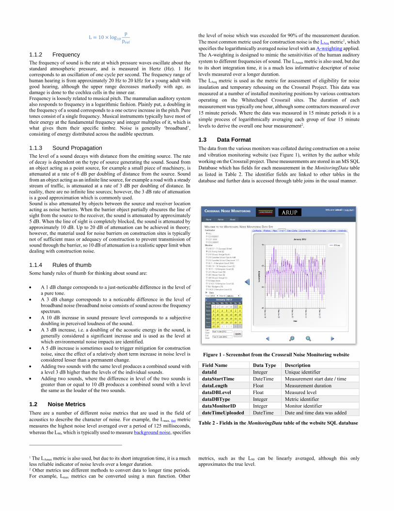
The data from the various monitors was collated during construction on a noise

and vibration monitoring website (see Figure 1), written by the author while

working on the Crossrail project. These measurements are stored in an MS SQL

Database which has fields for each measurement in the MonitoringData table

as listed in Table 2. The identifier fields are linked to other tables in the

database and further data is accessed through table joins in the usual manner.

Field Name Data Type Description

dataId Integer Unique identifier

dataStartTime DateTime Measurement start date / time

dataLength Float Measurement duration

dataDBLevel Float Measured level

dataDBType Integer Metric identifier

dataMonitorID Integer Monitor identifier

dateTimeUploaded DateTime Date and time data was added

Table 2 - Fields in the MonitoringData table of the website SQL database

metrics, such as the L90 can be linearly averaged, although this only

approximates the true level.

Figure 1 - Screenshot from the Crossrail Noise Monitoring website

1.4 Data Conversion

The data from the website was first standardised into one hour durations by

logarithmic averaging using another piece of software written by the author

(see Figure 2), which applies time and level filters to raw data. This was saved

as a single .csv file with fields as listed in Table 3.

Field Data Type Description

StartDateTime DateTime Measurement start date / time

EndDateTime DateTime Measurement end date / time

Duration Float Measurement duration

Level Float Measurement level

Metric String Metric Name

Filter String Filter used to derive the data

from raw format

Monitor String Name of measurement location

Table 3 - Intermediate data format output from VizAcoustics

The third and final stage of conversion was performed using a Python script,

which extracted the LAeq data from the single .csv file and wrote it to separate

.csv files, one for each monitor. The fields of these files are shown in Table 4.

The monitor and duration fields were no longer necessary as each file

represents a single measurement location, and all derived measurements are of

one hour duration.

Field Data Type Description

Level Float Measured level

Year Integer Year of measurement

Month Integer Month of measurement

Day Integer Day of measurement

Hour Integer Start hour of measurement

Table 4 - Fields of .csv files used for analysis in Noise Cluster program

1.5 Data Description

Ten measurement locations were available for analysis. However, due to time

constraints, three locations were selected to illustrate and test the methodology.

These are shown in Figure 3. Measurements were available during different

date periods at each monitor, so a date period of 27th February 2012 to 30th November 2013 was chosen, as data was available at all three locations during

this period.

Figure 3 - Aerial View of Whitechapel Worksites and Selected

Measurement Locations (imagery from Google Maps)

1.5.1 Albion Yard (East)

The Albion Yard (East) measurement location is located on the site boundary of the eastern Cambridge Heath Shaft Worksite at ground floor level. It is

located to monitor noise to the Albion Medical Centre and the east side of the

Albion Yard residential building to the south on Whitechapel Road. Its primary noise sources in the absence of construction noise are Whitechapel Road and

Cambridge Heath Road.

1.5.2 Albion Yard (North)

The Albion Yard (North) measurement location is located on the site boundary

of the western Cambridge Heath Shaft Worksite at first floor level. It is located to monitor noise to the north side of the Albion Yard residential building. Its

primary noise sources in the absence of construction noise are Brady Street and

Cambridge Heath Road.

1.5.3 Trinity Hall (East)

The Trinity Hall (East) measurement location is located on the eastern façade of the Trinity Hall residential building, overlooking the Durward Street Shaft

and Whitechapel Station worksites. It is located on the rooftop of the building

(fourth floor level). Its primary noise sources in the absence of construction noise are Whitechapel Station and Whitechapel Road.

2 ANALYSIS TASKS

2.1 Clustering

The tasks used in the analysis relate primarily to the first case study chosen for the literature review [8]. The goal of the case study was to analyse daily

patterns of power consumption at the Energy Research Centre of the

Netherlands. The goal of this analysis was slightly more nuanced in that after identification of common daily or part-daily patterns (called “profiles” in this

report), it was necessary to try to find likely causes for some of them (e.g.

construction, bank holidays) and exclude them from analysis, so that the true

underlying typical ambient levels could be established. This required the

incorporation of some additional functionality, such as specification of the time period over which to perform the clustering as shown in Figure 4.

The clustering method used was hierarchical agglomerative clustering, as it

allows for changing the number of clusters in real time and is allows for more interactive than other types when processing power is limited.

Figure 2 - Screenshot of VizAcoustics noise processing software

Figure 4 - Clustering Settings Controls from the Noise Cluster program

for the Crossrail IP D9 Periods 1 – 3

2.2 Visualisation and Analysis of Clusters

The screenshots in the case study only showed visualisation of clusters via the calendar view and the cluster representatives line graph. In order to gain further

insight into the nature of clusters, the following additional views were

included:

Distance between clusters, and change in the inter-cluster distance

gradient for each number of partitions in the clustering.

Number of members of each cluster.

Number of members of each cluster over each month of the clustering.

2.3 Cluster modification

Although members of clusters (profiles) are by definition more similar to each other than to member of other clusters, there are additional restrictions imposed

by the noise insulation policy, (e.g. weekday levels should not include bank

holidays), that necessitated the ability to remove members of clusters that fell on these days. These days were removable by clicking on them whilst holding

the control key. This functionality, in conjunction with the profiles view, also

allows users to remove specific members from a cluster if they are considered to be outliers in comparison to other members of the cluster.

2.4 Cluster Correlation

The case study indicated that next steps for the program would enable users to

study “several variables simultaneously in order to study correlations between

variables, either manually or automatically”. Functionality was added to the Noise Cluster program to export two types of cluster representatives, which

were then analysed offline using Python scripts. These representative-types are

as follows:

Best-fit profile using polynomial curve-fitting.

Modal profile using the most frequently occurring levels at each hour.

3 ANALYSIS METHODOLOGY

The analysis methodology was inspired by the case study and modified

according to the overall aim of the analysis. Some of the methods used were identical or very similar, such as:

Visualisation of the individual profiles.

Clustering of the data.

Selection of appropriate clusters.

Subsequent cluster analysis by correlation.

Other additional steps were introduced, both to better facilitate the analysis and to improve interactivity. These steps are described in the following subsections.

3.1 Clustering Settings

The clustering settings are set by the user before loading the data. The settings

are as given in Table 5:

Setting Description

Method Clustering method to use (single, complete, average,

weighted, centroid, median, ward)

First Date The first date of the clustering period

Last Date The last date of the clustering period

Start Hour The start hour on each day of clustering

End Hour The end hour on each day of clustering (if the end hour

is less than or equal to the start hour then this falls on the next day)

Days Days of the week from which clustering is calculated

Table 5 - Clustering settings configurable by the user for each clustering

3.2 Clustering

The clustering is performed by the computer on initial loading of the data, and

upon user request. Reclustering is required when the user wants to change the clustering method, or alter the time or date periods or days of the week over

which the clustering is performed. Reclustering takes between 2 and 10

seconds on the author’s relatively low specification laptop for the full date range, depending on the number of days of the week clustered, and the length

of time period for each day.

3.3 Cluster Visualisation

Once the clustering calculation has been completed, the computer sets the

number of clusters to one, and colours each day of the calendar in blue, indicating that they all belong to the same unified cluster. The Clusters tab

graphs are updated with the cluster distances and gradient changes, the cluster

representative, the number of members and the monthly distribution over the clustering date range. The computer also highlights all public holidays in a bold

italic font, so they are more easily distinguishable from other days.

3.4 Selection of Correct Number of Clusters

The user increases the number of clusters, using the spinbox in the

Visualisation Controls toolbox, either by clicking the up and down arrows or by typing in the number directly. This second option can save time if there is a

noticeable sharp change in the Inter-Cluster Distance, or a peak in the Inter-

Cluster Distance Gradient Change at a specific number of clusters, because the computer needs to update the cluster graphs and calendar view colours each

time the number of clusters is changed.

The correct number of clusters needs to be determined by the user. This involves consideration of a number of factors, such as:

Domain knowledge about the likely ambient profile, taking into account the ambient noise sources in the area

Changes in the distance between cluster members for each cluster

Shapes of profiles in the clustering, and the number of days on which

each cluster profile occurs.

Monthly and seasonal distributions of each cluster

The shapes of individual profiles within each cluster

The temporal proximity of individual profiles to public holidays

Figure 5 shows a typical view after increasing the number of clusters to five.

Figure 5 - Initial Clustering of IP D9 Time Periods 1-3. The most likely

ambient levels are represented by the blue cluster

3.5 Removal of cluster members

Outliers may be detected in a cluster by inspection of the individual profiles

for each cluster. These can subsequently be removed by control-clicking on the

day in the calendar view, or by simply increasing the number of clusters until the outlier separates from the cluster of interest. This needs to be done by the

user as it can be a matter of judgement as to what constitutes an outlier. The

user can also consult other documents, such as project work diaries and other publicly available information to ascertain the causes of anomalous profiles.

Figure 6 - Profiles of the ambient cluster selected, with bank holidays

deselected manually by the user in the calendar view

3.6 Choosing Cluster Representatives

The Cluster Representatives graph on the Clusters tab, shows the mean level for each cluster over each hour of the day. However, when cluster members are

removed from consideration by the user, this plot does not update because it

would involve recomputation of the entire clustering. To address this issue, the user can visualise the data for all the selected days on the Cluster

Representative tab.

Since the goal of the analysis is to find the typical ambient levels, not the average ambient levels, it was decided not to use the mean or median levels in

this plot. Two other approaches were used instead.

The first approach is to fit a polynomial curve to the data to generate a line of best-fit that minimises the squared error between the curve and the measured

points for each hour. The order of the polynomial is three by default, but can

be changed by the user by using the spinbox provided in the Visualisation Controls toolbox.

The second approach is to find the modal level for each hour of the day. This

is achieved by putting each level into a histogram bin and finding the bin with the most members. The binning interval is 0.1 dB by default, but can be

modified by the user in 0.1 dB increments by using a spinbox in the

Visualisation Controls toolbox. Once the cluster representatives have been chosen, the user exports them to

.csv files for subsequent analysis. Figure 7 shows a view of polynomial and

modal best-fit lines.

Figure 7 - Polynomial and modal best-fit lines for ambient cluster

members. The backdrop shows the distribution of noise levels for each

hour in 1dB bins

4 IMPLEMENTATION

All of the analysis, with the exception of the correlation, was performed in the Noise Cluster program, which was modified and improved as the analysis was

conducted and shortcomings were identified. This section describes the

program and its constituent parts, and the standard libraries that were used to assist in calculations and visualisations.

4.1 Software Development Environment

The environment chosen to develop the software was Eclipse, using the PyDev

add-on. Toolboxes and layouts were designed using the Qt Designer program.

Standard “widgets” were used for most views, apart from the Clustering Calendar View, which was inherited from a QTableView. The programming

paradigm used was a variation on the Model-View-Presenter pattern. UML

Class diagrams for the views and view models are shown in Figure 8 and Figure 9.

Figure 8 - UML Class Diagram for View Classes

Figure 9 - UML Class Diagram for ViewModel Classes

4.2 Standard Modules

The following Python modules were used to assist in implementation of the program:

Module Use

PyQt4 Graphical User Interface

Event Handling (signals and slots)

numpy Array handling and manipulation

pandas Internal data representation

Data file import / export

datetime, dateutil Date handling and offsetting

pickle Loading and saving of settings files

math Rounding of numbers for binning

matplotlib Plots

scipy Clustering

Polynomial approximations

Table 6 - List of standard Python modules used in Noise Cluster

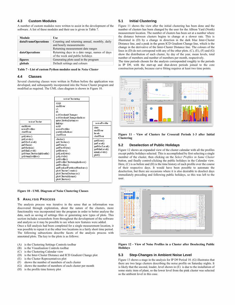
4.3 Custom Modules

A number of custom modules were written to assist in the development of the

software. A list of these modules and their use is given in Table 7.

Module Use

dataFrameOperations Counting and returning annual, monthly, daily and hourly measurements

Returning measurement date ranges

dateOperations Returning days in a date range, names of days

of the week and public holidays

figures Generating plots used in the program

globals Default settings and colours

Table 7 - List of custom Python modules used in Noise Cluster

4.4 Classes

Several clustering classes were written in Python before the application was

developed, and subsequently incorporated into the Noise Cluster program and modified as required. The UML class diagram is shown in Figure 10.

Figure 10 - UML Diagram of Noise Clustering Classes

5 ANALYSIS PROCESS

The analysis process was iterative in the sense that as information was

discovered through exploration, about the nature of the clusters, more functionality was incorporated into the program in order to better analyse the

data, such as saving of settings files or generating new types of plots. This

section includes screenshots from throughout the development of the software and analysis so it may be possible to see when new features were added.

Once a full analysis had been completed for a single measurement location, it

was possible to repeat it at the other two locations in a fairly short time period. The following subsections describe facets of the analysis process with

annotated plots. The key to the plots is as follows:

(A) is the Clustering Settings Controls toolbar (B) is the Visualisation Controls toolbar

(C) is the Clustering Calendar view (D) is the Inter-Cluster Distance and ICD Gradient Change plot

(E) is the Cluster Representatives plot

(F) shows the number of members of each cluster (G) shows the number of members of each cluster per month

(H) is the profile time history plot

5.1 Initial Clustering

Figure 11 shows the view after the initial clustering has been done and the

number of clusters has been changed by the user for the Albion Yard (North)

measurement location. The number of clusters has been set at a number where the distance between clusters begins to change at a slower rate. This is

illustrated in (D) by a change in direction in the dark blue Inter-Cluster

Distance line, and a peak in the green ICD Gradient Change line, which is the change in the derivative of the Inter-Cluster Distance line. The colours of the

lines in (D) do not correspond with any of the other plots. (C), (E), (F) and (G)

show the distribution of each cluster, by day of the year, mean levels, total number of members and number of members per month, respectively.

The time periods chosen for the analysis corresponded roughly to the periods

in IP D9, with the start-up and shut-down periods joined to the core construction periods, because curve fitting requires at least two time points.

Figure 11 - View of Clusters for Crossrail Periods 1-3 after Initial

Clustering

5.2 Deselection of Public Holidays

Figure 12 shows an expanded view of the cluster calendar with all the profiles except public holidays selected. This is accomplished by first selecting a single

member of the cluster, then clicking on the Select Profiles in Same Cluster

button, and finally control-clicking the public holidays in the Calendar view. Here, (C) is as before and (H) is the time history of each profile over the course

of their respective days. It would have been possible to automate the

deselection, but there are occasions where it is also desirable to deselect days immediately preceding and following public holidays, so this was left to the

user.

Figure 12 - View of Noise Profiles in a Cluster after Deselecting Public

Holidays

5.3 Step-Changes in Ambient Noise Level

Figure 13 shows a stage in the analysis for IP D9 Period 10. (G) illustrates that

there are two large clusters describing the noise profile on Saturday nights. It

is likely that the second, louder, level shown in (E) is due to the installation of some static item of plant, so the lower level from the pink cluster was selected

as the ambient level in this case.

Figure 13 - Step-Change in Typical Ambient Noise Level

5.4 Inherent Variation in Ambient Noise Levels

For some time periods, the analysis showed a high degree of inherent variation

in the natural ambient noise level, independent of any construction noise

contribution. This can be seen in Figure 14 by the similarly shaped profiles for

the IP D9 Period 12 Sunday night-time period in (E). In this case, the yellow

level was selected as the typical cluster, because it first occurs at the start of the clustering (G), is similarly persistent to the pink cluster and is at a lower

level so errs on the side of caution when dealing with third parties.

However this does pose the question as to whether there is truly a “typical” ambient noise level for some time periods or whether it varies as new sources

are introduced. This is more likely to happen at quieter time periods such as

Sunday night times because the overall ambient noise level is lower and therefore prone to being more affected by other sources due to the logarithmic

summing of noise.

Figure 14 - Clustering for Sunday nights shows four potential "typical"

ambient noise level profiles

5.5 Influence of Local Sources on Typical Noise Levels

It was found whilst analysing the Trinity Hall East measurement location that

typical ambient levels were much easier to establish than at the Albion Yard

locations. This is because it directly overlooks two railway lines. Since

railways have regular schedules with specific numbers of trains and

announcements per hour, the hourly noise levels are much more consistent than

at other locations. The orange cluster in Figure 15 is by far the most frequently occurring one (F).

The blue and pink clusters represent periods where there is either a reduced or

cancelled service due to public holidays (C). This raises the issue that there may not be a single typical level for public holidays adjacent to certain types

of environmental noise source.

Figure 15 - Distribution of Typical Ambient Noise Levels adjacent to the

Railway

5.6 Selection of Cluster Representatives

As previously discussed, two methods were used to select representative levels

for ambient clusters. Each one has its strengths and weaknesses.

5.6.1 Polynomial Curve Fitting

The polynomial curve fitting method has the advantage that by specifying the

order of the polynomial, the user can tailor the shape of the curve to have as

many changes in direction as desired. The disadvantage of this approach is that it could be criticised as a somewhat arbitrary method of selecting the ambient

level; two different experts could easily come up with different levels, which

would not be beneficial for establishing agreement between parties with differing priorities.

In addition to this, it was found during experimentation that when longer time

periods are clustered, the polynomial curve fitting approach may fit the data well at the hours of the clustering, but that it does not behave well inbetween

or outside these periods, as shown in Figure 16. This means that when clusters

are joined together, the joins can be very obvious, which gives them an artificial look, even if the underlying mean squared error between the curve and the

levels has been reduced.

Figure 16 - Deviation of Polynomial Approximation outside Hours of

Clustering

5.6.2 Modal Levels

One of the advantages of the modal levels approach is that there is a direct analogy between the modal level and the typical level, so it is easier to justify

to residents and other laypeople who may be interested in the analysis why it

has been selected. Although there is a loss of accuracy from binning levels, it is common practice to report measured levels to the nearest decibel. Therefore,

as long as the bin size is less than or equal to 1 dB, then there is no loss in

reported accuracy. Also, Type 1 sound level meters (the most accurate class) are only required to be accurate to ± 1 dB, and Type 2 to the ± 2 dB, so the

measurement error is likely to be higher than the analysis error.

One of the major disadvantages is that for smaller bin sizes, the number of

levels in each bin is small, so it is more difficult to make the case for the selected level being typical. For larger bin sizes, where the size is less than 1

dB, the modal level is less smooth in appearance than the fitted line, and can

be subject to sudden apparent “jumps”. This phenomenon will be discussed further in Section 6, but can be seen at 12pm in Figure 17 below, where the

typical level appears to jump up to around 64 dB, even though there is a

relatively highly populated bin around 60 dB which would make a smoother profile.

Figure 17 - Illustration of the 'jump' phenomenon for modally derived

noise profiles

6 RESULTS AND CONCLUSIONS

6.1 Results

6.1.1 Noise Profiles

Noise profiles for the three locations analysed on Weekdays, Saturdays and Sundays derived from best-fit lines and modal levels are shown in Figure 18

and Figure 19.

Figure 18 - Ambient noise profiles derived from best-fit lines

Figure 19 - Ambient noise profiles derived from modal levels

Overall, the noise profiles represent good and similar estimations of the

ambient noise levels without the presence of construction noise. However, due

to the choice to analyse the levels using time windows derived from the noise

insulation policy, there are marked changes in curve gradient at the boundaries

of some of the time periods used in Figure 18, due to the curve fitting algorithm

used. These may indicate some inaccuracies in the estimated noise levels at

certain hours of the day. The profiles derived from the modal levels do not

exhibit such obvious transitions, although they are subject to their own

irregularities, such as the “jump” in noise level at 12pm in the Albion Yard

East Weekdays plot. This happens when there are two competing levels within

a time period, and the one which fits better with the trend is slightly less

populous than the other. On balance, it is considered that the modal

representation is superior because it does not make any prior assumptions on

the noise profile and is more easily explainable to the layman as the “typical”

level as opposed to some mathematical approximation.

6.1.2 Cross Correlation

It would be expected that noise profiles from locations with similar ambient noise climates would exhibit a higher cross-correlation than areas with

different ambient noise climates. Similar noise climates at two locations may

be due to proximity to each other and consequently to similar local noise sources, or due to similarity to each other in terms of line of sight to significant

correlated noise sources, such as major roads.

Polynomial Approximation

Table 8 shows the cross-correlation between each position from the profiles

derived using the polynomial approximation technique.

Day Type Location Albion

Yard East

Albion

Yard

North

Trinity

Hall East

Weekdays A.Y.E. 1 0.97 0.95

A.Y.N 0.97 1 0.98

T.H.E 0.95 0.98 1

Saturdays A.Y.E. 1 0.96 0.95

A.Y.N 0.96 1 0.93

T.H.E 0.95 0.93 1

Sundays A.Y.E. 1 0.89 0.92

A.Y.N 0.89 1 0.93

T.H.E 0.92 0.93 1

Table 8 - Cross correlation between profiles derived using polynomial

approximations

Weekday ambient noise level exhibit very high correlations between all

locations. This suggests that noise from typical weekday activities such as road

traffic noise from commuters and commercial deliveries on the nearby A11

(Whitechapel Road) and A107 (Cambridge Heath Road) has a large influence

on ambient noise levels throughout the area.

On Saturdays, the correlation between noise levels at Trinity Hall East and

Albion Yard North is slightly lower. This is likely to be due to Albion Yard

North not having a direct line of sight to Whitechapel Road, which has a

number of restaurants, shops, pubs and a market, which contribute to the noise

climate.

On Sundays, noise levels at Trinity Hall East are not well correlated with either

of the Albion Yard locations. This suggests that due to the lower levels of

ambient noise from commercial and leisure activities, local noise sources have

more of an effect on the noise profile in each location. Noise levels at Albion

Yard are also very poorly correlated on Sundays. This is mostly due to the

increase in noise levels around 10pm at Albion Yard East. The cause of this

increase is unknown, but is possibly due to customers using the beer-garden of

the pub adjacent to the monitor.

Modal Levels

Table 9 shows the cross-correlation between the typical noise profiles for each measurement location derived using modal levels.

Day Type Location Albion

Yard East

Albion

Yard

North

Trinity

Hall East

Weekdays A.Y.E. 1 087 0.88

A.Y.N 0.87 1 0.94

T.H.E 0.88 0.94 1

Saturdays A.Y.E. 1 084 0.90

A.Y.N 0.84 1 0.82

T.H.E 0.90 0.82 1

Sundays A.Y.E. 1 0.82 0.86

A.Y.N 0.82 1 0.88

T.H.E 0.86 0.88 1

Table 9 - Cross correlation between profiles derived using modal levels

It is clear from a quick comparison of the two tables that the correlation between modal levels is much lower than using the polynomial approximation

technique. This is partially caused by the more “spiky” nature of binned levels,

and the “jump” phenomenon described in 5.6.2 and 6.1.1. However, ignoring the relative comparison between the two tables and viewing the modal

correlations in isolation, the lowest correlation coefficient between any two

locations is 0.84, which indicates that they are indeed describing similar profile shapes, as evidenced by the profile plots.

6.2 Conclusions

The advantage of an analysis using long-term measurements is that it is easier

to establish a typical level where one exists. However, the ambient noise

climate in any area is subject to change, for example due to introduction of new noise sources such as a new shop opening or a road closure in another area

directing traffic to nearby roads. These changes may be independent of the construction project, or indirectly related to the project. Such changes make it

more difficult to establish the typical ambient noise profile in the location.

However, using the software developed, it is much easier to see when the changes occurred, whether they are temporary, permanent or seasonal, as well

as what times of day they occur at. This makes it easier to find explanations for

the changes and should therefore make it easier to make a cogent argument to interested parties about what the typical levels are.

Further, the analysis has found that there may be many levels that could be

judged to be typical of the noise climate at a given location, particularly at times of the day or night where the overall ambient noise level is low, and

therefore any small local changes have a bigger effect on the noise level.

6.3 Further Work

The analysis is based on assumption that the time periods used in the IP D9

policy are appropriate time periods because they are organised both around the hours of working, and typical hours of waking and sleeping from other

legislation. However, this assumption may not be correct in the second respect,

as much of the legislation was developed a long time ago before the introduction of more flexible working hours. A future analysis could use

clustering of different time periods to determine which fall more naturally into

clusters. Further, if the technique used here were used in advance of construction, i.e.

based on ambient data only, other time periods might be more appropriate for

the purpose of analysis, before arranging the relevant noise levels into the periods required in the relevant policy document.

There also remain a number of enhancements that could be made to the

program, such as:

Automatic detection of cluster outliers using rules defined or

configurable by the user

Add cluster standard deviations or variances to cluster plots for better interpretation

Incorporate correlation analysis into the software for faster analysis

7 REFERENCES

[1] Various, “High Speed 1 Wikipedia Page,” Wikipedia, 20 April 2015.

[Online]. Available: http://en.wikipedia.org/wiki/High_Speed_1. [Accessed 20 Aptil 2015].

[2] Crossrail, “Crossrail Web Site,” Crossrail, 20 April 2015. [Online].

Available: http://www.crossrail.co.uk/. [Accessed 20 April 2015].

[3] T. T. Tunnel, “Thames Tideway Tunnel Website,” Thames Tideway

Tunnel, 20 April 2015. [Online]. Available:

http://www.thamestidewaytunnel.co.uk/. [Accessed 20 April 2015].

[4] U. Government, “Control of Pollution Act 1974,” 20 April 2015.

[Online]. Available: http://www.legislation.gov.uk/ukpga/1974/40.

[Accessed 20 April 2015].

[5] Crossrail, “Crossrail Information Paper D9,” 20 Novermber 2007.

[Online]. Available: http://74f85f59f39b887b696f-

ab656259048fb93837ecc0ecbcf0c557.r23.cf3.rackcdn.com/assets/library/document/d/original/d09noiseandvibrationmitigationscheme1.pdf.

[Accessed 20 April 2015].

[6] British Standards Institute, BS 5228 Code of practice for noise and vibration control on construction and open sites. Part 1: Noise, British

Standards Institute, 2009.

[7] British Standards Institute, BS 4142 - Method for Rating Industrial Noise Affecting Mixed Residential and Industrial Noise Areas, British

Standards Institute, 1997.

[8] J. J. van Wijk and E. R. van Selow, “Cluster and Calendar based Visualization of Time Series Data,” San Francisco, 1999.

[9] International Electrotechnical Commission, IEC 61672 Electroacoustics

- Sound level meters. Part 1: Specifications, International Electrotechnical Commission, 2013.