Food Marketing Policy Center

Determining the Impact of Retailer Store Brand Procurement on Vertical Relationships

with Brand Manufacturers and on Market Equilibrium

by Michael A. Cohen

Food Marketing Policy Center Research Report No. 122

January 2010

Research Report Series http://www.fmpc.uconn.edu

University of Connecticut Department of Agricultural and Resource Economics

Determining the Impact of Retailer Store Brand Procurement on

Vertical Relationships with Brand Manufacturers and on Market

Equilibrium †

Michael A. Cohen

University of Connecticut

Food Marketing Policy Center

This Version: January 7, 2010

Abstract

This paper investigates how a retailer’s store brand supply source impacts vertical pricing

and supply channel profitability. Using chain-level retail scanner data from major supermarkets

in Boston prior to the leading retailer’s divestiture of its store brand milk processing to a major

brand manufacturer I estimate a random coefficients logit demand model employing a Bayesian

estimation approach. Bayesian decision theory is applied to select from a set of pricing games

the one most likely for the data sample analyzed. Results from this analysis indicate that the

empirically valid model has the pre-divested retailer integrated into the processing of its own

milk and takes as given the wholesale price of brand milks while competing retailers have non-

linear pricing contracts with brand manufacturers who produce their store brands. This model

is matched against a series of counterfactual simulations as a baseline. The counterfactual sim-

ulations consider the eventual divestiture of store brand milk processing by the leading retailer

†I thank Alessandro Bonanno, Ron Cotterill, Jean-Pierre Dube, Avi Goldfarb, Renna Jiang, Adam Rabinowitz,Peter Rossi, Sylvie Tchumtchoua, and Gautam Tripathi for valuable discussions, comments, and information leadingto improvements in this paper. Any errors are my own.

to a major brand manufacturer as well as two fictional markets where store brands are no longer

offered and optimal nonlinear pricing breaks down making way for a double marginalization out-

come. Simulation results indicate that the divesture likely improved profitability and reduced

retail prices by eliminating double marginalization.

1 Introduction

In some cases retailers produce their own store brand products and in other cases they contract

production of their store brands to manufacturers who supply similar branded products. This

paper demonstrates that store brand procurement by supermarkets determines strategic pricing

arrangements with brand manufacturers. Both theoretical and empirical research finds that the

marketing of store brands by retailers eliminates double marginalization, reduces retail prices on

leading brands, and increases channel profits and consumer welfare. Store brand marketing as a

competitive strategy yields larger profit flow to the retailers generated by larger margins on the

leading manufacturer brands and the sale of store brands themselves (Mills, 1995; Scott-Morton

& Zettelmeyer, 2001; Chintagunta & Bonfrer, 2002). This paper employs a structural modeling

approach to analyze the vertical relationships of retailers and manufacturers when a leading super-

market processes its own store brand product and other supermarkets procure own-labeled milk

from brand manufacturers.

The investigation examines chain-level retailer scanner data for white fluid milks sold at

major supermarkets in Boston from March 1996 to July 2000. Specification of pricing models for

empirical testing requires estimation of an demand model. The flexible random coefficient logit

demand model of Berry, Levinsohn, and Pakes (1995) is applied and estimated using the Bayesian

approach of Jiang, Manchanda, and Rossi (2009). Parameter estimates are used to calculate implied

retailer and manufacturer margins under the alternative vertical pricing arrangements.

Channel costs are computed from the implied margins and regressed on input prices. Bayesian

decision theory selects the “best fitting” channel marginal cost model. If there are different pricing

relationships between supermarkets that manufacture their own store brands and supermarkets

that source store brands from brand manufacturers then the best fitting model will reveal them.

After finding empirical evidence that testifies that there are differences in pricing arrange-

2

ments for supermarket that produce their own store brands I consider counterfactuals that examine

differences to equilibria that result when the retailer divest processing of this store brand prod-

ucts to brand manufacturers. One of the counterfactuals considers the divestiture of the leading

retailer’s store brand processing to the leading brand manufacturer. The other two counterfactuals

investigate the market without store brands. In one case retailers and manufacturers engage in

nonlinear pricing. In the other case linear pricing leads to the double marginalization outcome that

store brand provision is thought to eliminate. I compute the percent difference in price, market

share, and consumer surplus between the selected market model and each counterfactual market

model to evaluate the impact of store brand supply source.

Mills (1995) presents a rigorous model that demonstrates store brands are instruments for a

retailer to overcome the well-known double marginalization problem present in distribution chan-

nels. Store brand provision allows the retailer to extract profit from the vertical channel and lower

prices. Steiner (2004) similarly argues that the unique position of store brands constrain the market

power of national brands in ways that their horizontal competitors cannot. Steiner (1993) describes

a vertical structure where store brands generate countervailing retailer power and improve welfare.

However neither of these papers considers how the retailers supply source impacts these effects.

An empirical analysis by Raju, Sethuraman, and Dhar (1995) finds that store brands increase

category profits for retailers and find that this is particularly true when a category has several

brands. Chintagunta and Bonfrer (2002) examine the introduction of a store brand into a category

by estimating demand conditions before and after its introduction at a single retailer. They observe

wholesale prices paid by the retailer and use them to gain intuition on vertical conduct in the

market. For demand they investigate the changes in preferences under the two market regimes,

before and after the introduction of the store brand. On the supply side they measure the effects of

the new entrant’s store brand on the actions between retailer and manufacturer. However they use

a conduct parameter approach and do not explicitly formulate and test alternative pricing games.1

Modeling the vertical channel allows the researcher to identify the nature of vertical pricing

conduct between manufacturers and retailers. These models link manufacturers wholesale pricing

moves down to some form of retailer pricing conduct. Sudhir (2001) demonstrates the need to1See Corts (1998) for critiques of conduct parameter approaches.

3

accurately model vertical strategic interactions along with horizontal strategic interactions when

using retail level data. Villas-Boas and Zhao (2005) investigate the ketchup market in a Texas

market and reveal bias that results by ignoring endogeneity of demand, and model the supply side

with the profit maximizing decision of retailers and manufacturers. Villas-Boas (2007) outlines

conditions that allow data on retail price, retail quantities and input prices at the two stages in

the market channel to identify retailers’ and manufacturers’ vertical pricing conduct. This method

allows one to investigate interactions in the market channel pricing using retail level prices without

observing wholesale prices. However she analyzes retail conduct for two chain stores and a small

retailer, a total of 3 locations, and a set of manufacturers. A thorough investigation of product the

market requires one to study a robust cross section of firms at each level of the channel. In this

paper I analyze vertical conduct in a market that has four retail chains, a total of 187 locations, each

chain with a store brand, and two brand manufactures that sell in all four retailers. Bonnet and

Dubois (2010) empirically investigate vertical contracts between retailers and manufactures using

retail data on bottled water collected from retail chains in France. They extend previous work by

considering non linear vertical contracts that model two part tariffs with and without retail price

maintenance.

Empirical models of the vertical channel estimated with retail scan data apply non-nested

tests between competing models of channel cost to determine a “best fitting” model. Villas-Boas

(2007) and Bonnet and Dubois (2010) use the tests of Smith (1992) and Voung (2002), Rivers

and Voung (2002) respectively to determine the best fitting channel cost model. The tests they

implement have two problems. One they are not transitive. Non-transitivity implies that the tests

of channel pricing potentially offer inconclusive and inconsistent results. Applying the Bayesian

framework directs the researcher to rank models according to posterior probability and select the

model with the highest probability guaranteing transitivity. The second problem those two papers

face is the identification strength on their non-nested testing approach. Testing models of channel

cost rely on the decomposition of price into retailer markup, manufacturer markup, and channel

cost, none of which are directly observed in retail scanner data. Therefore one requires exogenous

variation in at least two of the three components to achieve identification. The previous literature

does not exploit independent retailer specific variation in cost factors, implying their tests may not

4

be identified, at least in an nonparametric sense.

This paper contributes to the existing literature in two ways. Primarily it provides a frame-

work to analyze the impact of retailer store brand procurement on vertical pricing arrangements

and documents the extent two which a retailer’s supply source for store brands impacts market

equilibria. As an additional contribution this paper improves the approach for selecting the best

fitting model of supply channel pricing in two ways. First it overcomes the non-transitivity of the

non-nested tests, typically applied, by using Bayesian decision theory. Second it exploits retailer

level variation in product characteristics to establish identification of the tests for competing models

of market conduct.

The remainder of this paper is organized as follows. Next it introduces the Boston fluid

milk market and describes the data. Then it derives models for optimal retailer and manufacturer

margins and describes the set of market structures tested as potential candidates. The fourth section

presents the demand model, estimation approach, and method for model selection. The fifth section

presents the estimation results and model selection results. The sixth section compares the market

equilibrium for the selected model to the market equilibria that arise under the counterfactual

markets. Finally, concluding remarks and suggestions for extending the research are made.

2 The Boston Fluid Milk Market and Data

2.1 Facts About the Market for Fluid Milk in Boston

The Boston supermarket industry is one of the most competitive, ranking 6th among all IRI defined

marketing areas in the United States in grocery sales. 80% of food in Boston is sold though super

markets. Four major chains operate in most of the market: Stop & Shop, Demoulas Market

Basket, Shaw’s, and Star Market. Stop & Shop is the market share leader and enjoyed a significant

expansion during the study period. Stop & Shop captured this share from residual retailers while

the other supermarkets maintained their market share position.

Stop & Shop is owned and controlled by European retailing giant Royal Ahold. Shaw’s

is owned and controlled by a British company named Sainsbury PLC. Star Market was highly

leveraged but in the third quarter of 1998 they were bought out by Sainsbury PLC. After this

5

point Shaw’s and Star Market continued to operate under their respective banners. Since consumers

viewed these supermarkets as different retailers they are considered separate firms for this analysis.

The fourth supermarket, Demoulas, is a privately held retail chain.

Within the greater Boston IRI area Star Markets has larger presence in the inner city areas

with relatively smaller retail outlet size. Demoulas are primarily located in suburbs north of Boston

proper. Shaw’s and Stop & Shop are scattered throughout the market area, however Shaw’s has

fewer stores in the urban core.

The Boston fluid milk market has two primary brands, Garelick and Hood. Each retailer

sells a store brand. Store brands hold a dominant market share position within each retailer, this is

particularly true at Demoulas and Stop & Shop. Other milks on retailer shelves are fringe specialty

milks such as lactose intolerant and organic brand alternatives, whose popularity had not yet gained

momentum in the late 1990’s.

The Garelick brand manufacturer, Suiza, is the largest in the Boston area followed by Hood.

The store brand milk sold at Demoulas, Star Market, and Shaw’s is processed at Suiza plants. The

store brand milk sold at Stop & Shop was processed at a retailer owned plant. As of June 2000

Stop & Shop closed this plant and has since procured its store brand milk from Suiza’s processing

plants.

2.2 The Data

The Information Resources Inc.(IRI) Boston market level data for each of four chains used in this

study has many chain level variables including prices and quantity, and it covers 58 quad week

periods beginning March 1996 and ending July 2000. The class one raw milk price data are from

federal milk market order one publications. Data on supermarket characteristics for each chain

come from Spectra Marketing and span the same time period as the scanner data in quarterly

observations, this data set also reports a figure for sales per square foot. Per capita income and

population data have been collected from annual editions of Market Scope. Data on electricity and

diesel fuel cost are from the Energy Information Administration.2

2Spectra Marketing is a sister company of A. C. Nielsen. All marketing data are available from the University ofConnecticut, Food Marketing Policy Center.

6

Exploring chain level data implies uniform pricing behavior across retail outlets within a

chain in a market such as Boston. Generally for an advertised product such as milk this is the case

within a market area. Chains price uniformly to avoid the criticism that they are price gouging

particular urban neighborhoods. We aggregate IRI stock keeping unit (sku) data to the brand level

for each chain.3 We control for the impact of package size differences on demand by including a

units per volume variable in our demand specification. Aggregation over different fat levels, for a

given brand of white fluid milk is a reasonable practice because the retailers we consider engage in

flat pricing of milk across fat levels (Cotterill, Rabinowitz, Cohen, Murphy, & Rhodes, 2007).

The same brands at different retailers are different products. For this reason our demand

specification includes attributes of the retail chain as a characteristic of the products purchased

in that retail chain. Using Spectra Marketing data one has the following retailer characteristics:

pharmacy, bank, fresh fish counter, deli, and salad bar. This approach recognizes that a chain

can brand it self by developing a unique array of services and products including a broad high

quality line of store brands. Also chain specific data generate exogenous variation in retail margins

that permit us to identify the non-nested tests of channel pricing conduct. Bonnano and Lopez

(2009) report that the consumer demand for fluid milk is influenced by one stop shopping attributes

of supermarkets including breadth and depth of services offered. In the Spectra data one knows

whether a specific store in the Boston market has the service or not. Using this information one

can calculate the proportion of stores in the chain offering the service in each time period. Due

to collinearity in the service data I use principal component analysis to identify two orthogonal

services. To generate a non-food service variable I take the product of the propensity measures for

those services, the same procedure is executed to generate a food service variable.

Table 1 reports summary statistics for chain specific brand price, market shares, and group

shares. Hood has the highest per gallon prices across all chains followed by Garelick then private

label. Among the retail chains Star Markets, located in the urban core, has on average the highest

milk prices followed by Stop & Shop, Shaws, then Demoulas. Stop & Shop has the largest share of

fluid milk sales with 18%, and they lead in store brand sales with 12.6% while Demoulas is a close

second with 11.1%. Store brand dominates sales within Demoulas at 89.8% whereas Star markets3Skus identify package sizes and different products within a brand.

7

store brand milk sales only make up 52.3%.

Table 2 has summary statistics for three other control variables. Weighted price reduction

is a variable measuring price promotion of a given brand in the supermarket. It is the percent

reduction in price from the suggested retail price when price is reduced. This variable controls for

price promotional activities. The “share of skim to whole milk sold” controls for the aggregation of

the different butter fat content milks which may influence demand if consumers are health conscious.

A value greater than 1 reveals that a greater share of skim or low-fat milk was sold for the given

product than whole. “Units per volume” which is the average number of units sold per gallon and

controls for container size.

Table 3 reports the Spectra Marketing data on store characteristics for each chain. Stop&Shop

had on average approximately 70 stores in the Boston metropolitan area during this period, Shaws

had approximately 46, Demoulas 32 and Star 19. Stop&Shop’s stores have the most retail space.

Stop&Shop is also the leader in services especially in non-food services as compared to their com-

petitors. Demoulas has the fewest services and Shaws and Star have similar amounts. Table 3 also

has market level statistics for household income as well as channel input costs: the prices of raw

milk, electric, and diesel. Note the typical price paid to farmers for a gallon of raw milk is $1.40

effectively half of the retail price.

3 Structural Model of the Supply Channel

This section introduces the supply models tested as candidates for the Boston fluid milk market.

Strategic profit maximization is modeled at both the retail and manufacturer levels of the supply

chain. Farmers supply milk at an exogenously set federal milk market order prices, so manufacturers

secure it from a competitive input market. First I derive profit maximizing margins for retailers

and then for manufacturers under linear pricing. Next I introduce a model for nonlinear contracts

in the form of two part tariffs. Then I argue for a set of six empirical models tested as relevant

candidates for the Boston fluid milk market.

8

3.1 Linear Pricing

Retailer

Assume there are N Nash Bertrand multi-product oligopolists competing in a retail market and

each retailer maximizes category profit for sale of all branded and own-labeled fluid milk products.

Each retailer’s milk profit function, for a particular time period, is:

πr = maxpj∀j∈Sr

∑j∈Sr

[pj − pmj − crj ]sj(p).

Sr is the set of products sold by retailer r, m indexes manufacturers and j indexes products. The

first order condition, assuming a pure strategy Nash equilibrium in prices, is:

sj +∑k∈Sr

[pk − pmk − crk]∂sk∂pj

= 0. (1)

The first order conditions can be stacked into a system of equations for each product at each retailer.

The terms may be rearranged to solve for retailer margins. This linear system can be expressed in

matrix notation:

p− pw − cr = −(Tr ×elt 4r)−1s(p). (2)

Tr is a matrix of ones and zeros that captures the products in the set Sr by executing element-

wise multiplication, ×elt. In other words the retailers maximize their profits over products in their

portfolio, hence its called the ownership matrix. Element Tr(k, j) = 1 if a retailer has both products

k and j in their portfolio, and Tr(k, j) = 0 otherwise. 4rt is a matrix containing the derivatives

of share with respect to retail price. This matrix is called the retailer response matrix and has the

typical element ∂sj

∂pk.

Manufacturer

Assuming that manufacturers set wholesale price upon observing retail price the manufacturer’s

profit maximization problem is written as:

πm = maxpm∀j∈Sm

∑j∈Sm

[pmj − cmj ]sj(p(pm)).

9

Here Sm is the set of products sold by manufacturer m. The resulting first order condition is:

sj +∑k∈Sm

[pmk − cmk ]∂sk∂pmj

= 0. (3)

The manufacturer ownership matrix Tm is defined in a manner analogous to that of the retail

ownership matrix. The elements of the manufacturer response matrix, 4m, are the derivatives of

product market share with respect to wholesale price, i.e. ∂sj

∂pmi

. The matrix 4m contains the cross

price elasticities of demand and the effects of cost pass through, these effects can be decomposed

in the following manner by evoking the chain rule:

4m = 4′p4r.

Here 4p represents the cost pass through and 4r contains own and cross price sensitivities of

market share to retail price changes. 4r was introduced in the previous subsection. The matrix

4p’s elements are the derivatives of all retail prices with respect to all wholesale prices, and have

the general element 4p(k, j) = ∂pj

∂pmk

.

The elements of the matrix 4p are derived by totally differentiating, for a given product j,

the retailer first order condition in equation 1:

N∑k=1

[∂sj∂pk

+N∑i=1

(Tr(i, j)∂2si∂pj∂pk

(pi − pmi − cri )) + Tr(k, j)∂sk∂pj

]︸ ︷︷ ︸g(j,k)

dpk − Tr(f, i)∂sf∂pj︸ ︷︷ ︸

h(j,f)

dpmf = 0.

Stacking these conditions for all j = 1, 2, ..., N products together into a linear system, one has,

Gdp−Hfdpmf = 0.

The matrix G has general element g(j, k), and Hf is an N -dimensional vector with general element

h(j, f). Rearranging terms implies the vector,

dp

dpmf= G−1Hf .

10

Horizontally concatenating Hf together for all products j, one has the desired matrix,

4p = G−1H.

Collecting terms equation 3 is solved for the manufacturers’ implied price-cost margins:

pmt − cmt = −(Tw ×elt 4m)−1s(p). (4)

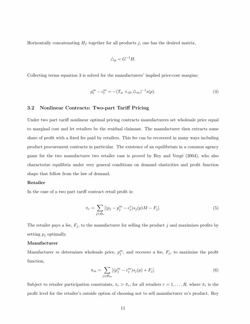
3.2 Nonlinear Contracts: Two-part Tariff Pricing

Under two part tariff nonlinear optimal pricing contracts manufacturers set wholesale price equal

to marginal cost and let retailers be the residual claimant. The manufacturer then extracts some

share of profit with a fixed fee paid by retailers. This fee can be recovered in many ways including

product procurement contracts in particular. The existence of an equilibrium in a common agency

game for the two manufacturer two retailer case is proved by Rey and Verge (2004), who also

characterize equilibria under very general conditions on demand elasticities and profit function

shape that follow from the law of demand.

Retailer

In the case of a two part tariff contract retail profit is:

πr =∑j∈Sr

[(pj − pmj − crj)sj(p)M − Fj ]. (5)

The retailer pays a fee, Fj , to the manufacturer for selling the product j and maximizes profits by

setting pj optimally.

Manufacturer

Manufacturer m determines wholesale price, pmj , and recovers a fee, Fj , to maximize the profit

function,

πm =∑j∈Sm

[(pmj − cmj )sj(p) + Fj ]. (6)

Subject to retailer participation constraints, πr > πr, for all retailers r = 1, . . . , R, where πr is the

profit level for the retailer’s outside option of choosing not to sell manufacturer m’s product. Rey

11

and Verge (2004) show that the participation constraints must be binding otherwise manufacturer

fees Fj would rise only to be bounded by the conduct of other manufacturers. Bonnet and Dubois

(2010) show that the expression for Fj can be substituted into equation 6 to recover the profit for

manufacturer m:

πm =∑j∈Sm

(pj − crj − cwj )sj(p) +∑j 6∈Sm

(pj − pwj − crj)−∑j 6∈Sm

Fj ] (7)

This expression reveals that manufacturers internalize the full margins on their products but only

the retail margins on other manufacturers products. The additional term∑

j 6∈SmFj is constant

for manufacturer m and consequently drops out of the profit maximization problem which implies

that impled channel markup is:

p− cr − cw = −(Tr ×elt δr)−1s(p). (8)

Under this arrangement the retailer recovers profits of a vertically integrated structure for the j

products in its portfolio and manufacturers recover a share of these profits in the form of fees, Fj ,

or contracted wholesale prices.

Villas-Boas (2007) and Bonnet and Dubois (2010) consider a case where retail margins are

zero and manufacturers make pricing decisions and award retailers slotting fees for selling their

product or engage in resale price maintenance. Bonnet and Dubois (2010) test this model for the

French bottled water market as two part tariff pricing with resale price maintenance. This model

will not be considered for the Boston fluid milk market owing to legal standards on retail price

maintenance.

3.3 Empirical Models of Channel Pricing

An empirical test to select the best fitting vertical pricing model enables one to determine whether

retailer store band procurement arrangements impact pricing relationship with brand manufac-

turers. This paper tests six distinct structural models of pricing conduct which are identified by

implied channel margins from a set of pricing games. Specification of the ownership matrices, Tr

12

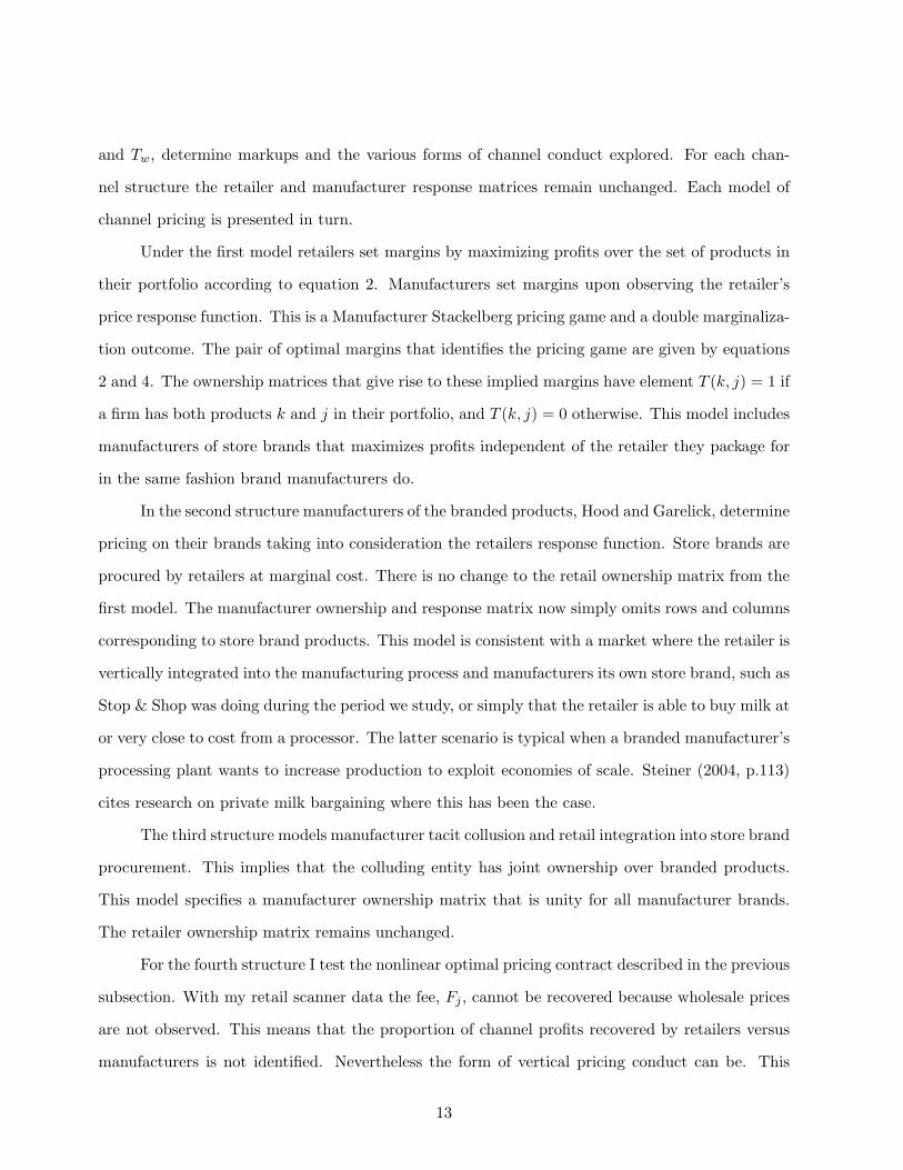
and Tw, determine markups and the various forms of channel conduct explored. For each chan-

nel structure the retailer and manufacturer response matrices remain unchanged. Each model of

channel pricing is presented in turn.

Under the first model retailers set margins by maximizing profits over the set of products in

their portfolio according to equation 2. Manufacturers set margins upon observing the retailer’s

price response function. This is a Manufacturer Stackelberg pricing game and a double marginaliza-

tion outcome. The pair of optimal margins that identifies the pricing game are given by equations

2 and 4. The ownership matrices that give rise to these implied margins have element T (k, j) = 1 if

a firm has both products k and j in their portfolio, and T (k, j) = 0 otherwise. This model includes

manufacturers of store brands that maximizes profits independent of the retailer they package for

in the same fashion brand manufacturers do.

In the second structure manufacturers of the branded products, Hood and Garelick, determine

pricing on their brands taking into consideration the retailers response function. Store brands are

procured by retailers at marginal cost. There is no change to the retail ownership matrix from the

first model. The manufacturer ownership and response matrix now simply omits rows and columns

corresponding to store brand products. This model is consistent with a market where the retailer is

vertically integrated into the manufacturing process and manufacturers its own store brand, such as

Stop & Shop was doing during the period we study, or simply that the retailer is able to buy milk at

or very close to cost from a processor. The latter scenario is typical when a branded manufacturer’s

processing plant wants to increase production to exploit economies of scale. Steiner (2004, p.113)

cites research on private milk bargaining where this has been the case.

The third structure models manufacturer tacit collusion and retail integration into store brand

procurement. This implies that the colluding entity has joint ownership over branded products.

This model specifies a manufacturer ownership matrix that is unity for all manufacturer brands.

The retailer ownership matrix remains unchanged.

For the fourth structure I test the nonlinear optimal pricing contract described in the previous

subsection. With my retail scanner data the fee, Fj , cannot be recovered because wholesale prices

are not observed. This means that the proportion of channel profits recovered by retailers versus

manufacturers is not identified. Nevertheless the form of vertical pricing conduct can be. This

13

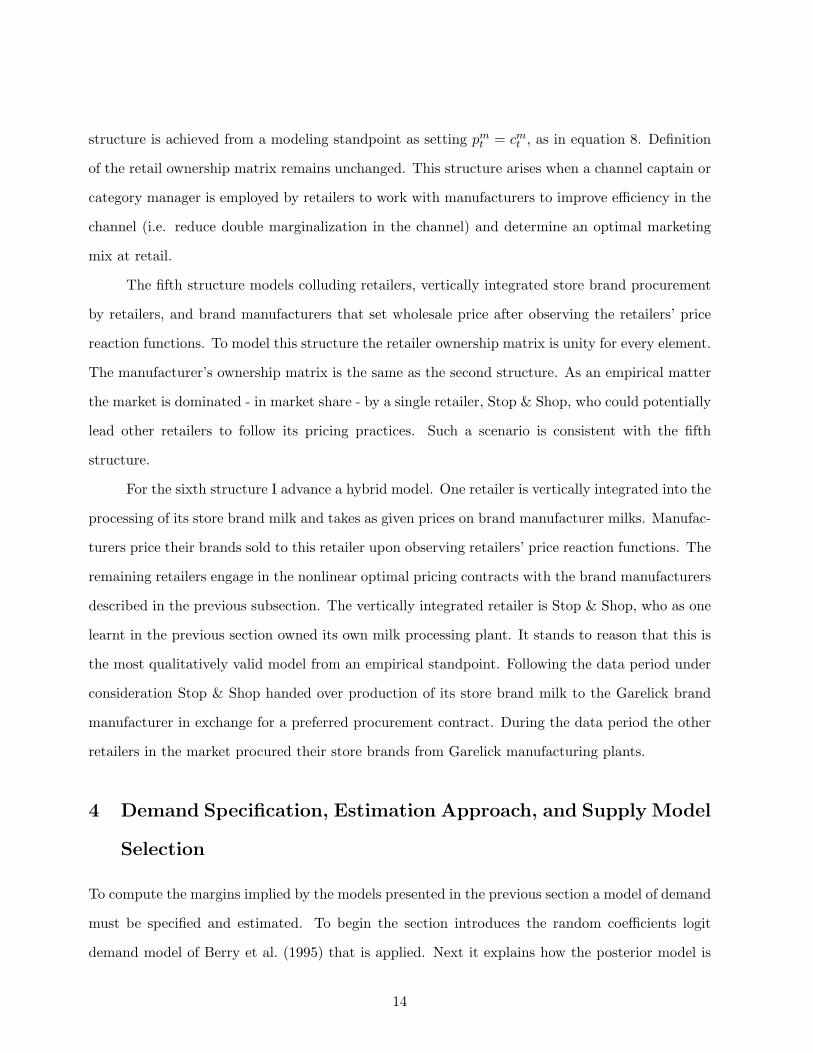
structure is achieved from a modeling standpoint as setting pmt = cmt , as in equation 8. Definition

of the retail ownership matrix remains unchanged. This structure arises when a channel captain or

category manager is employed by retailers to work with manufacturers to improve efficiency in the

channel (i.e. reduce double marginalization in the channel) and determine an optimal marketing

mix at retail.

The fifth structure models colluding retailers, vertically integrated store brand procurement

by retailers, and brand manufacturers that set wholesale price after observing the retailers’ price

reaction functions. To model this structure the retailer ownership matrix is unity for every element.

The manufacturer’s ownership matrix is the same as the second structure. As an empirical matter

the market is dominated - in market share - by a single retailer, Stop & Shop, who could potentially

lead other retailers to follow its pricing practices. Such a scenario is consistent with the fifth

structure.

For the sixth structure I advance a hybrid model. One retailer is vertically integrated into the

processing of its store brand milk and takes as given prices on brand manufacturer milks. Manufac-

turers price their brands sold to this retailer upon observing retailers’ price reaction functions. The

remaining retailers engage in the nonlinear optimal pricing contracts with the brand manufacturers

described in the previous subsection. The vertically integrated retailer is Stop & Shop, who as one

learnt in the previous section owned its own milk processing plant. It stands to reason that this is

the most qualitatively valid model from an empirical standpoint. Following the data period under

consideration Stop & Shop handed over production of its store brand milk to the Garelick brand

manufacturer in exchange for a preferred procurement contract. During the data period the other

retailers in the market procured their store brands from Garelick manufacturing plants.

4 Demand Specification, Estimation Approach, and Supply Model

Selection

To compute the margins implied by the models presented in the previous section a model of demand

must be specified and estimated. To begin the section introduces the random coefficients logit

demand model of Berry et al. (1995) that is applied. Next it explains how the posterior model is

14

specified for the Boston market data examined by applying the method of Jiang et al. (2009). Then

it explains the Bayesian decision theoretic approach employed for selecting the most likely channel

supply model.

4.1 Random Coefficients Logit

The random coefficients logit allows consumers to differ in tastes for product characteristics. In-

troducing heterogeneity in this way allows for flexibility in substitution patterns overcoming the

restrictive substitution patterns implicit in simple logit or nested logit demand models. Implied

margins computed free of the preordained substitution patterns guarantee that supply model se-

lection is not driven by a restrictive demand specification.

I specify the following linear version of the random utility model(RUM)

Vij = Xjβi − αipj + ηj + εij (9)

i and j subscript individuals and products respectively. A product is defined as a unique brand -

retailer combination. xj is a vector of characteristics for product j, and pj is the price of product

j. ηj is an aggregate brand and retailer specific demand shock, or in other words, a time varying

product attribute unobserved by the econometrician. It is assumed that εij are distributed i.i.d.

according to an extreme value type I distribution. There are J products and a zero utility outside

option, i.e. a consumer has the option of not buying milk at any of the retailers. [βi, αi] ≡ θi are

marginal utility parameters assumed to vary over consumers and follow the multivariate-normal

distribution, θi ∼ N([θ,Σ).

The market share of product j as a function of the total group share is

sj =∫sijφ(θi|θ,Σ)dθi.

=∫

exp(Xjθi + ηj)

1 +∑

k exp(Xkθi + ηk)φ(θi|θ,Σ)dθi (10)

where φ is the multivariate normal density. Predicted shares can be expressed in terms of mean

15

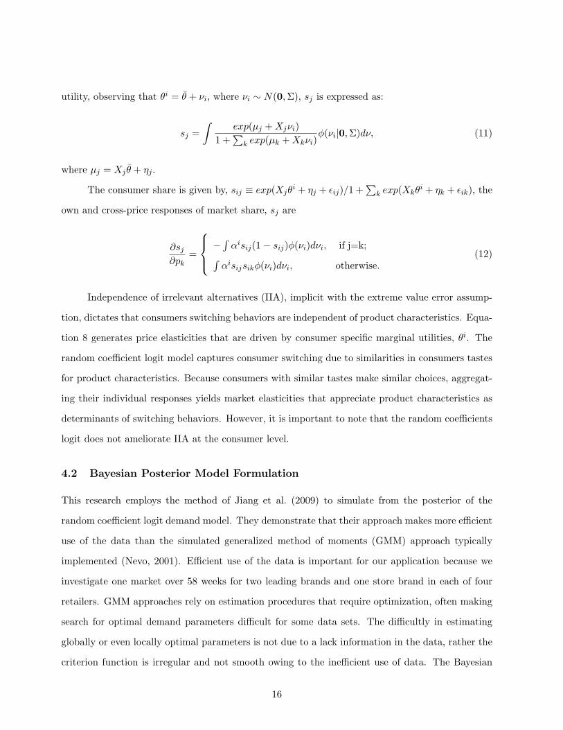
utility, observing that θi = θ + νi, where νi ∼ N(0,Σ), sj is expressed as:

sj =∫

exp(µj +Xjνi)1 +

∑k exp(µk +Xkνi)

φ(νi|0,Σ)dν, (11)

where µj = Xj θ + ηj .

The consumer share is given by, sij ≡ exp(Xjθi + ηj + εij)/1 +

∑k exp(Xkθ

i + ηk + εik), the

own and cross-price responses of market share, sj are

∂sj∂pk

=

−∫αisij(1− sij)φ(νi)dνi, if j=k;∫

αisijsikφ(νi)dνi, otherwise.(12)

Independence of irrelevant alternatives (IIA), implicit with the extreme value error assump-

tion, dictates that consumers switching behaviors are independent of product characteristics. Equa-

tion 8 generates price elasticities that are driven by consumer specific marginal utilities, θi. The

random coefficient logit model captures consumer switching due to similarities in consumers tastes

for product characteristics. Because consumers with similar tastes make similar choices, aggregat-

ing their individual responses yields market elasticities that appreciate product characteristics as

determinants of switching behaviors. However, it is important to note that the random coefficients

logit does not ameliorate IIA at the consumer level.

4.2 Bayesian Posterior Model Formulation

This research employs the method of Jiang et al. (2009) to simulate from the posterior of the

random coefficient logit demand model. They demonstrate that their approach makes more efficient

use of the data than the simulated generalized method of moments (GMM) approach typically

implemented (Nevo, 2001). Efficient use of the data is important for our application because we

investigate one market over 58 weeks for two leading brands and one store brand in each of four

retailers. GMM approaches rely on estimation procedures that require optimization, often making

search for optimal demand parameters difficult for some data sets. The difficultly in estimating

globally or even locally optimal parameters is not due to a lack information in the data, rather the

criterion function is irregular and not smooth owing to the inefficient use of data. The Bayesian

16

Markov Chain Monte Carlo (MCMC) methods used by Jiang et al. (2009) to estimate the random

coefficient logit do not require optimization and are insensitive to simulation error. The tradeoff is

to specify a distribution on the common demand shock. They show that their estimator performs

well even when demand shock distribution is misspecified. In this subsection the likelihood is

derived and the priors are introduced.

Recognizing the endogeneity of price I employ an instrumental variable approach. This

requires specifying a recursive system containing the price and share equations. The price equation,

pjt = Zjtδ + ξjt, (13)

specifies price, pjt, as a function of instrumental variables, Zjt, and additive error, ξjt, where t

indexes data observations. The share equation can be specified solely as a function of the aggregate

shock ηt = (η1t, . . . , ηJt)′, given the distribution of θi and observed regressors Xt = (X1t, . . . , XJt).

The density of shares can be written as a function of the demand shock density. The function

relating demand shock to shares is given by h(·):

sjt = h(ηt|Xt, θ,Σ). (14)

Endogeneity of price implies that the random shocks ξjt are correlated with the demand

shocks ηjt according to the following multivariate-normal density:

ξjt

ηjt

∼ N 0

0

, Ω ≡

Ω11 Ω12

Ω21 Ω22

. (15)

Up to this point the model is identical to that of Berry et al. (1995). The additional assump-

tion necessary to specify the likelihood is a distributional assumption on the demand shock. The

demand shocks are specified as independently distributed and homoscedastic. The joint density of

17

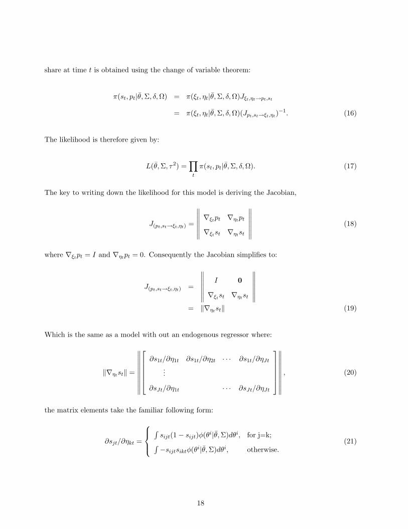
share at time t is obtained using the change of variable theorem:

π(st, pt|θ,Σ, δ,Ω) = π(ξt, ηt|θ,Σ, δ,Ω)Jξt,ηt→pt,st

= π(ξt, ηt|θ,Σ, δ,Ω)(Jpt,st→ξt,ηt)−1. (16)

The likelihood is therefore given by:

L(θ,Σ, τ2) =∏t

π(st, pt|θ,Σ, δ,Ω). (17)

The key to writing down the likelihood for this model is deriving the Jacobian,

J(pt,st→ξt,ηt) =

∥∥∥∥∥∥∥∇ξtpt ∇ηtpt

∇ξtst ∇ηtst

∥∥∥∥∥∥∥ (18)

where ∇ξtpt = I and ∇ηtpt = 0. Consequently the Jacobian simplifies to:

J(pt,st→ξt,ηt) =

∥∥∥∥∥∥∥I 0

∇ξtst ∇ηtst

∥∥∥∥∥∥∥= ‖∇ηtst‖ (19)

Which is the same as a model with out an endogenous regressor where:

‖∇ηtst‖ =

∥∥∥∥∥∥∥∥∥∥

∂s1t/∂η1t ∂s1t/∂η2t · · · ∂s1t/∂ηJt

...

∂sJt/∂η1t · · · ∂sJt/∂ηJt

∥∥∥∥∥∥∥∥∥∥, (20)

the matrix elements take the familiar following form:

∂sjt/∂ηkt =

∫sijt(1− sijt)φ(θi|θ,Σ)dθi, for j=k;∫−sijtsiktφ(θi|θ,Σ)dθi, otherwise.

(21)

18

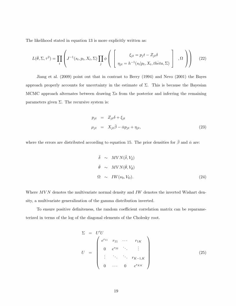
The likelihood stated in equation 13 is more explicitly written as:

L(θ,Σ, τ2) =∏t

J−1(st, pt, Xt,Σ)∏j

φ

ξjt = pjt− Zjtδ

ηjt = h−1(st|pt, Xt, ¯theta,Σ)

,Ω

(22)

Jiang et al. (2009) point out that in contrast to Berry (1994) and Nevo (2001) the Bayes

approach properly accounts for uncertainty in the estimate of Σ. This is because the Bayesian

MCMC approach alternates between drawing Σs from the posterior and inferring the remaining

parameters given Σ. The recursive system is:

pjt = Zjtδ + ξjt

µjt = Xjtβ − αpjt + ηjt, (23)

where the errors are distributed according to equation 15. The prior densities for β and α are:

δ ∼ MVN(δ, Vδ)

θ ∼ MVN(θ, Vθ)

Ω ∼ IW (ν0, VΩ). (24)

Where MVN denotes the multivariate normal density and IW denotes the inverted Wishart den-

sity, a multivariate generalization of the gamma distribution inverted.

To ensure positive definiteness, the random coefficient correlation matrix can be reparame-

terized in terms of the log of the diagonal elements of the Cholesky root.

Σ = U ′U

U =

er11 r11 · · · r1K

0 er22. . .

......

. . . . . . rK−1,K

0 · · · 0 erKK

(25)

19

where r = rjkj,k=1,...,K,j≤k. r’s prior densities are

rjj ∼ N(0, σr jj), for j=1,. . . ,K;

rjk ∼ N(0, σr off ), for j,k=1,. . . ,K,j¡k.(26)

All the priors I introduce are implemented with standard diffuse settings, the specific values used

are presented in the next section on data, estimation, and results.

4.3 Supply Model Selection

In keeping with my estimation approach I formally rank the models of supply side conduct using

Bayesian decision theory. This process allows me to rank the models and select the most probabilis-

tic model. I begin by specifying models of channel pricing. Then I implement a Bayesian modeling

approach to compute posterior model marginal densities, subsequently used for model selection.

The margins can be specified in a model of channel pricing as:

pjt = RMjt +MMjt +

ChannelCost︷︸︸︷Zjtγ +εijt. (27)

The implied price-cost margins for the six pricing games laid out in the previous section specify six

competing models of channel pricing. The implied margins can be subtracted from both sides of

equation 27 to define a channel cost specification for each pricing game:

pjt −RMijt −MMijt = CCijt = Zjtγi + εijt. (28)

This is the channel cost model for pricing game i. RM is the retail margin and MM is the

manufacturer margin.

The channel pricing model specified in equation 24 parallels that of Villas-Boas (2007) and

Bonnet and Dubois (2010). They estimate each channel cost model separately and conduct pair-

wise non-nested tests to identify the models that best explain the data generation process, which

arguably are the most likely supply channel models. The non-nested tests they employ are not

transitive. For example consider three possible models. If model 1 is chosen in favor of model 2

20

and 2 is chosen in favor of 3 it is not guaranteed that 1 is chosen in favor of 3.

Bayesian decision theory for model selection strictly ranks the models under consideration,

bypassing the non-transitivity issue. If prior densities are the same for each model considered,

Bayesian decision theory directs the researcher to select the most probabilistic model based on

exact sample results. I compute posterior model probabilities directly and rank models from most

to least probabilistic. I evaluate the model level error likelihoods under the following specification:

εijt = pjt −RMjt −MMjt − Zjtγ,

εijt ∼ N(0, κ). (29)

Here γ is the posterior estimate. My test exploits the temporal scedasticity within each panel of

the cross section of models. Marginal density estimates are computed for the posterior error model

in equation 28 to determine the best fitting pricing model.

5 Estimation and Model Selection Results

This section presents the specification of demand variables, demand parameter estimates, and

results for the model selection exercise.

5.1 Specification, Estimation, and Parameter Estimates

To begin specification of the demand model market shares must be computed. To compute shares I

assume that each member of Boston’s population consumes 8 ounces of fluid milk each day.4 Larger

and smaller markets were considered but did not change elasticity estimates in a significant way,

verifying the robustness of parameter estimates under different exogenously determined market

sizes. Given actual consumption and total potential consumption one can compute the market

share of the outside good as well as the shares for different brands of milk sold in the different

chains. The Independent variables specified in the random coefficients logit demand equations

product characteristics including: weighted price reduction, share of skim to whole, as well as food

and non-food services that the supermarkets offered.48 ounces is the recommended serving size for a glass of milk as stated on milk packaging

21

I employ the instrumental variable technique described in the previous section to identify α,

the coefficient on the endogenous price variable. The price endogeneity control function specifies

price as a function of channel input prices. The specification input prices considered are the price

of raw milk multiplied by the brand indicator variables, price of electric, diesel, and retailer sales

per square foot .5

We use diffuse prior setting for all model priors. All priors are proper, that is they have a

probability measure of one over their support. All slope parameters have a prior mean of 0 and

prior variance of 100 ∗ Ik, where Ik is an identity matrix of dimension k, equal to the number of

slope parameters. Recall that error variance Ω has an inverted Wishart density with:

ν0 = k + 1 and VΩ =

1 0.5

0.5 1

(30)

The prior setting for r, the demand parameter covariance matrix elements have mean 0 and variance:

σ2rjj =

14log

1 +√

1− 4(2(j − 1)σ4roff− c)

2

, (31)

where σ2roff

= 1 and c = 50. This specification of priors for r ensures that the priors associated

with the correlations are uniformly distributed between 0 and 1 (Jiang et al., 2009, p.146-147).

Table 4 presents market mean parameter estimates, θ, standard deviation of the posterior

distribution of θ and numerical standard errors for the distribution estimates for the simple logit

and random coefficient logit demand model. Simulation of the market share integral for the random

coefficients logit from equation 11 is achieved by simulating 100 households, the literature com-

monly uses between 50 and 100 households. Jiang et al. (2009) document that the Bayes sampling

properties are virtually unchanged when increasing the number of households from 50 to 200.

Here we discuss the random coefficients logit demand coefficients. The marginal utility of

income parameter on price has the proper sign, adhering to the law of demand. The price reduction

coefficient is located near zero indicating that price promotions have no major impact on average5Interacting raw milk prices with brand dummies allows us to separate brand variation in prices (Villas-Boas,

2007, p.637-38).

22

consumption utility. The positive units per volume coefficient indicates that consumers prefer

smaller packaging per unit. The positive skim to whole ratio testifies that consumer prefer milk

with less fat on average. More services generate higher utility whether they are food or non-food

services. Below the demand parameter estimates appear estimates for the price endogeneity control

function and below them appear average estimates of error covariance.

Table 5 displays the average estimates for the covariance of θi, Σ, over the individuals in the

market. Variance estimates on the main diagonal of this matrix suggest there is a wide range of

preferences over package size as evidenced by a variance measure of more than 18. The variance of

nearly 79 on the food service marginal utility parameter suggest that a sizeable portion of consumers

in fact negatively value food service. The price coefficient has a standard deviation of approximately

7. Since the marginal distribution of the price parameter is centered about -43.395 effectively all of

the consumers in the market obey the law of demand. The fact that the highest degree of covariance

is between price and other product characteristics supports the notion that adjusting the product,

place, and promotion is an effective marketing technique to attract consumers who are less sensitive

to price.

5.2 Supply Model Test Results

Table 7 displays results from the set of channel marginal cost models introduced in section 3.

Coefficients on other regressors measure channel marginal costs sensitivity to changes in input

prices. Log marginal density estimates at the bottom of the table reveal that the channel pricing

game characterized by model 6 is the best fitting model. Recall from section 3 that model 6 seemed

most plausible ex ante based on a stylized assessment of Boston’s milk market. Given both forms

of analysis is stands to reason that model 6 best characterizes the market, and it establishes a

baseline from which to compare counterfactual market structures.

6 Counterfactual Simulation Analysis

The structural models of demand and supply are used in this section to conduct three counterfactual

simulations. I begin by introducing the simulation technique. Next I describe the counterfactuals.

23

Then I present the results of our simulations.

6.1 Technique

Given estimates of the structural parameters, ownership matrices, response matrices, market share,

and implied channel costs, equilibrium prices, p∗t , are determined by the following system of equa-

tions:

p∗t = M(Tr, Tw,4rt,4wt, st(p∗t )) + Ct. (32)

Where M(·) denotes the implied model for channel margins, Ct ≡ pt −M(. . . , st(pt) is channel

costs, and pt are observed prices. Counterfactual equilibria arise under alternative pricing games.

I determine the counterfactual equilibrium prices and shares, st(p∗t ), by specifying the appropriate

counterfactual ownership matrices, Tr and Tw, and response matrices,4rt and 4wt.

Given equilibrium prices that arise under a particular pricing game the change in consumer

surplus, CSt(pt) − CSt(p∗t ), is evaluated using the following formula for the random coefficients

logit demand model:

CSit(pt) =1|αi|

E [maxjVijt(pt)] =1|αi|

ln

J∑j=1

exp[Vijt(pt)]

. (33)

For the counterfactual games I evaluate firm specific margins are not always identified since I don’t

model the bargaining that occurs between retailers and manufacturers on nonlinear contracts and

I do not observe wholesale prices.

6.2 Counterfactuals

In the previous section Bayesian decision theory selects model six as most appropriate for this data

sample. Recall that model six has Stop & Shop integrated into its store brand production and

brand manufacturers Garelick and Hood set wholesale price as Stackelberg leaders, the remaining

retailers coordinate with the brand manufacturers. I simulate changes in price, market share, and

consumer surplus in the equilibrium framework described above, for three counterfactual scenarios.

The first counterfactual scenario I evaluate is the divestiture of Stop & Shop store brand

24

processing where they subsequently engage in a nonlinear contract with brand manufacturers as

other retailers were doing.

The second and third counterfactuals I evaluate are markets without store brands. In one

scenario all supermarkets make nonlinear contracts. In scenario two retailers and manufacturers

maximize profits independently with manufacturers as Stackelberg leaders. This is the double

marginalization outcome the presence of store brands has been credited with eliminating (Mills,

1995; Steiner, 2004). These two counterfactuals reveal the extent to which store brand presence

improves consumer welfare.

6.3 Results

Table 8 documents average percent changes in price, channel profits, market share, and consumer

surplus under each counterfactual. Sample standard deviation and sample standard error appear

beside each estimate of the mean change. Under scenario one Stop & Shop’s impending divestiture

promises to decrease prices on all fluid milks across the board. The steepest decline in price happens

in Stop & Shop for the brand milks. The Stop & Shop store brand increases in price, this result

suggests the effects of coordination are at work to increase the flow of profits to manufacturers

from milks sold in Stop & Shop. Changes in market share also testify to this fact owing to major

increases in the market shares of brand products at Stop & Shop, and a smaller decline in share

at other retailers. Ultimately, Stop & Shop’s divestiture of it’s processing plant results in a small

average net increase in consumer surplus.

The lower panels of table 8 display changes for the second and third scenarios. Under the

second scenario elimination of double marginalization through the Stop & Shop marketing channel

decreases prices on brand milks sold at Stop & Shop. However the net increase in prices across

all retailers results in an overall decrease in consumer surplus. If one believes that without store

brands the market would be characterized by double marginalization the third panel of table 9

offers the equilibrium differential. This grim possibility attests that prices would be higher across

the board and that consumer surplus would be dashed by nearly 94%.

25

7 Conclusion

This paper conducts an empirical examination of store brand marketing on vertical competition

among retailers and manufacturers. Estimating market demand provides parameter estimates used

to calculate channel profit margins under six alternative channel pricing games. From the channel

profit margins estimated we derived six alternative channel marginal costs models corresponding

to each supply channel pricing game. The model we determined to be most probable posits that

Stop & Shop was integrated into its own store brand processing and procured branded milks from

manufacturers who were setting wholesale prices to Stop & Shop as channel Stackelberg leaders

while the other retailers coordinated channel pricing with manufacturers. This result is consistent

with our institutional understanding of the Boston milk marketing channel.

Simulations found that Stop & Shop’s divestiture of its store brand milk processing to the

brand manufacturers likely lowered prices on all milks except Stop & Shop store brand resulting in

a marginal consumer welfare increase. Results also indicated that if store brands were not in the

market and the market was coordinated, prices would be higher at all retailers but Stop & Shop

and Consumer surplus would fall by nearly 30%. If store brands were absent from the market, and

double marginalization pricing emerged, prices increase across the board and consumer surplus is

dashed by nearly 94%.

Should post divesture data from the Boston milk market become available one can test for

structural changes in the market. Ultimately, availability of wholesale prices would enable one

to formally test the identification strategy used for model selection. It would also enable the

researcher to identify the transfer payments retailers make to brand manufacturers in the form of

channel coordinated wholesale price.

References

Berry, S., Levinsohn, J., & Pakes, A. (1995). Automobile Prices in Market Equilibrium. Econo-

metrica, 63, 841–889.

Berry, S. T. (1994). Estimating Descrete Choice Models of Product Differentiation. RAND Journal

26

of Economics, 25 (2), 242–262.

Bonnano, A., & Lopez, R. (2009). Competition Effects of Supermarket Services. American Journal

of Agricultural Economics.

Bonnet, C., & Dubois, P. (2010). Inference on Vertical Contracts Between Manufacturers and

Retailers Allowing for Non Linear Pricing and Resale Price Maintenance. RAND Journal of

Economics, 41 (1).

Chintagunta, P., & Bonfrer, A., I. S. (2002). Investigating the Effects of Store Brand Introduction.

Management Science, 48, 1242–1268.

Corts, K. S. (1998). Conduct parameters and the measurement of market power. Journal of

Econometrics, 88 (2), 227–250.

Cotterill, R. W., Rabinowitz, A. N., Cohen, M. A., Murphy, M. R., & Rhodes, C. R. (2007).

Toward Reform of Fluid Milk Pricing in Southern New England: Farm Level, Wholesale, and

Retail Prices in the Fluid Milk Marketing Channel. A report to the conencitcut legislature

committee on the environment, Food Marketing Policy Center, University of Connecticut.

Jiang, R., Manchanda, P., & Rossi, P. (2009). Bayesian analysis of random coefficient logit models

using aggregate data. Journal of Econometrics, 149 (2), 136–148.

Mills, D. E. (1995). Why Retailers Sell Private Labels. Journal of Economics and Management

Strategy, 1 (4), 509–528.

Nevo, A. (2001). Measuring Market Power in the Ready-to-Eat Cereal Industry. Econometrica,

69 (2), 307–342.

Raju, J., Sethuraman, R., & Dhar, S. (1995). The Introduction and Performance of Store Brands.

Management Science, 41 (6), 957–978.

Rey, P., & Verge, T. (2004). Resale Price Maintenance and Horizontal Cartel. Cmpo working paper

series 02/047, Bristol University, Center for Market and Public Organization.

27

Rivers, D., & Voung, Q. H. (2002). Model Selection Tests for Nonlinear Dynamic Models. The

Economics Journal, 5, 1–39.

Scott-Morton, F., & Zettelmeyer, F. (2001). The Strategic Positioning of store Brands in Retailer

Manufacturer Negotiations. Working paper, Yale University.

Smith, R. J. (1992). Non-Nested Tests for Competing Models Estimated by Generalized Method

of Moments. Econometrica, 60 (4), 973–80.

Steiner, R. L. (1993). The Inverse Association Between the Margins of Manufacturers and Retailers’.

Review of Industrial Organization, pp. 717–40.

Steiner, R. L. (2004). The Nature and Benefits of National Brand/Private Label Competition.

Review of Industrial Organization, pp. 105–27.

Sudhir, K. (2001). Strategic Analysis of Manufacturer Pricing in the Presence of a Stratigic Retailer.

Marketing Science, 20, 244–64.

Villas-Boas, J., & Zhao, Y. (2005). Retailer, manufacturers, and individual consumers: Modeling

the supply side in the ketchup marketplace. Journal of Marketing Research, 42 (1), 83–95.

Villas-Boas, S. B. (2007). Vertical Relationships Between Manufacturers and Retailers: Inference

with Limited Data. Review of Economic Studies, 74, 625–652.

Voung, Q. (2002). Likelihood Ratio Tests for Model Selection and Non-Nested Hypotheses. Econo-

metrica, 57, 307–333.

28

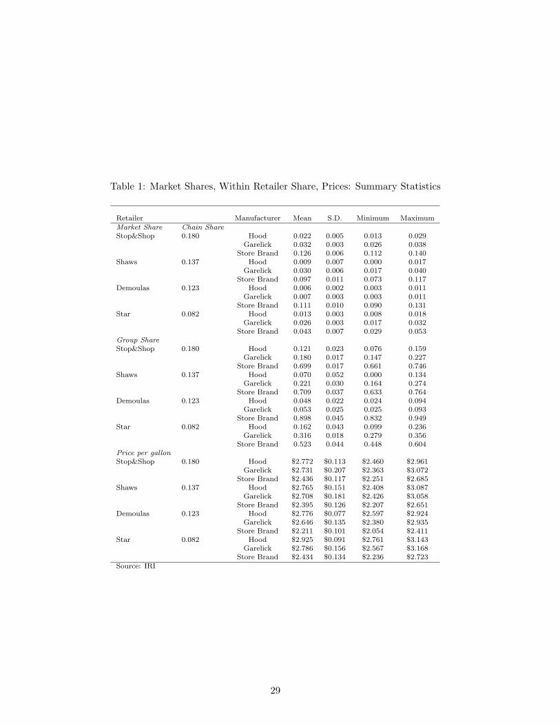
Table 1: Market Shares, Within Retailer Share, Prices: Summary Statistics

Retailer Manufacturer Mean S.D. Minimum MaximumMarket Share Chain ShareStop&Shop 0.180 Hood 0.022 0.005 0.013 0.029

Garelick 0.032 0.003 0.026 0.038Store Brand 0.126 0.006 0.112 0.140

Shaws 0.137 Hood 0.009 0.007 0.000 0.017Garelick 0.030 0.006 0.017 0.040

Store Brand 0.097 0.011 0.073 0.117Demoulas 0.123 Hood 0.006 0.002 0.003 0.011

Garelick 0.007 0.003 0.003 0.011Store Brand 0.111 0.010 0.090 0.131

Star 0.082 Hood 0.013 0.003 0.008 0.018Garelick 0.026 0.003 0.017 0.032

Store Brand 0.043 0.007 0.029 0.053Group ShareStop&Shop 0.180 Hood 0.121 0.023 0.076 0.159

Garelick 0.180 0.017 0.147 0.227Store Brand 0.699 0.017 0.661 0.746

Shaws 0.137 Hood 0.070 0.052 0.000 0.134Garelick 0.221 0.030 0.164 0.274

Store Brand 0.709 0.037 0.633 0.764Demoulas 0.123 Hood 0.048 0.022 0.024 0.094

Garelick 0.053 0.025 0.025 0.093Store Brand 0.898 0.045 0.832 0.949

Star 0.082 Hood 0.162 0.043 0.099 0.236Garelick 0.316 0.018 0.279 0.356

Store Brand 0.523 0.044 0.448 0.604Price per gallonStop&Shop 0.180 Hood $2.772 $0.113 $2.460 $2.961

Garelick $2.731 $0.207 $2.363 $3.072Store Brand $2.436 $0.117 $2.251 $2.685

Shaws 0.137 Hood $2.765 $0.151 $2.408 $3.087Garelick $2.708 $0.181 $2.426 $3.058

Store Brand $2.395 $0.126 $2.207 $2.651Demoulas 0.123 Hood $2.776 $0.077 $2.597 $2.924

Garelick $2.646 $0.135 $2.380 $2.935Store Brand $2.211 $0.101 $2.054 $2.411

Star 0.082 Hood $2.925 $0.091 $2.761 $3.143Garelick $2.786 $0.156 $2.567 $3.168

Store Brand $2.434 $0.134 $2.236 $2.723Source: IRI

29

Table 2: Promotion, Package Size, Skim to Whole Ratio: Summary Statistics

Retailer Manufacturer Mean Median S.D. Minimum MaximumWeighted Price ReductionStop&Shop Hood 8.33 7.78 5.30 0 22.89

Garelick 8.99 7.48 6.59 0 27.37Store Brand 8.29 8.30 3.19 0 16.68

Shaws Hood 7.42 8.29 7.17 0 26.83Garelick 11.48 12.18 5.54 0 24.89Store Brand 8.04 8.50 4.34 0 19.22

Demoulas Hood 1.86 0.00 3.00 0 7.00Garelick 2.08 0.00 3.16 0 11.16Store Brand 4.17 4.94 3.74 0 11.95

Star Hood 7.65 7.32 4.16 0 17.03Garelick 9.41 9.47 4.51 0 21.05Store Brand 5.50 5.93 3.23 0 12.75

Units per VolumeStop&Shop Hood 0.187 0.186 0.009 0.175 0.227

Garelick 0.187 0.186 0.006 0.175 0.213Store Brand 0.171 0.172 0.004 0.157 0.178

Shaws Hood 0.199 0.199 0.005 0.185 0.209Garelick 0.158 0.158 0.002 0.154 0.163Store Brand 0.277 0.264 0.026 0.239 0.318

Demoulas Hood 0.236 0.239 0.018 0.192 0.278Garelick 0.154 0.157 0.005 0.147 0.162Store Brand 0.288 0.292 0.013 0.265 0.306

Star Hood 0.201 0.201 0.006 0.185 0.214Garelick 0.165 0.166 0.002 0.160 0.172Store Brand 0.270 0.265 0.015 0.247 0.295

Skim to Whole RatioStop&Shop Hood 12.52 12.16 1.85 7.69 17.92

Garelick 16.53 16.31 2.13 11.11 22.08Store Brand 10.73 10.75 0.33 9.99 11.61

Shaws Hood 7.17 8.66 3.22 1.06 10.69Garelick 14.32 14.23 2.04 11.35 18.45Store Brand 11.57 11.47 0.70 10.25 12.73

Demoulas Hood 4.20 4.20 1.29 2.10 6.28Garelick 4.19 4.07 0.83 2.96 7.46Store Brand 12.47 12.43 0.38 11.80 13.54

Star Hood 8.53 8.93 2.39 4.94 14.41Garelick 14.13 13.77 2.16 10.45 20.73Store Brand 11.56 11.73 0.81 9.16 14.23

Source: IRI

30

Table 3: Income, Services, Cost Proxies and Input Costs: Summary Statistics

Retailer Variable Mean Median S.D. Minimum Maximum

Income $18,003 $17,894 $1,398 $16,240 $19,787

Stop&Shop Number of stores 69.65 70.5 4.40 61 74Bakery 0.861 0.888 0.056 0.730 0.904Bank 0.578 0.605 0.053 0.453 0.622Restaurant 0.043 0.054 0.017 0.015 0.057Pharmacy 0.567 0.599 0.075 0.423 0.649Seafood Counter 0.947 0.957 0.032 0.880 0.990Volume Sales 491559 509857 41520 426689 553425Retial Sq Footage 41178 42234 3293 33932 44730

Shaws Number of stores 46.45 46 1.61 43 49Bakery 0.924 1 0.123 0.708 1Bank 0.391 0.391 0.059 0.313 0.486Restaurant 0.064 0.066 0.048 0 0.136Pharmacy 0.055 0.043 0.026 0.019 0.093Seafood Counter 1 1 0 1 1Volume Sales 35388 36149 2528 30125 38111Retial Sq Footage 24991 24903 355 24465 25558

Demoulas Number of stores 32.1 32 0.31 32 33Bakery 0.544 0.588 0.093 0.352 0.633Bank 0.046 0.000 0.064 0.000 0.156Restaurant 0.055 0.062 0.013 0.031 0.063Pharmacy 0.017 0.000 0.028 0.000 0.063Seafood Counter 0.829 0.882 0.102 0.641 0.917Volume Sales 555204 566927 32652 497656 598438Retial Sq Footage 38641 40026 5496 27087 44781

Star Number of stores 39.25 39.5 2.75 33 42Bakery 0.978 1 0.032 0.920 1Bank 0.365 0.383 0.059 0.244 0.429Restaurant 0.180 0.173 0.078 0.095 0.360Pharmacy 0.370 0.382 0.047 0.273 0.424Seafood Counter 0.971 0.970 0.019 0.945 1Volume Sales 405614 419367 35431 327000 435888Retial Sq Footage 35260 34617 2756 32196 41819CostsPrice of raw Milk $1.40 $1.39 $0.10 $1.23 $1.66Electric $7.67 $7.86 $0.93 $5.19 $9.27Diesel $112.42 $113.21 $12.23 $89.33 $131.72

Source: Income: Market Scope, Retailer Characteristics: Spectra Marketing,Costs: Federal Milk Market Order and Energy Information Association

31

Table 4: Posterior Model Mean Parameter EstimatesLogit Random Coefficients Logit

Variable coefficient s.d. n.s.e. coefficient s.d. n.s.e.

Demandprice -33.000 2.000 0.0150 -43.395 4.557 0.5011price reduction 0.001 0.005 0.0000 -0.006 0.014 0.0018units per volume 3.464 0.648 0.0043 3.720 1.487 0.1470skim to whole ratio -7.963 0.264 0.0017 0.093 0.030 0.0042food service 1.715 0.200 0.0015 2.142 0.615 0.0764non food service -0.597 0.470 0.0037 4.123 1.237 0.1524constant 2.475 0.418 0.0030 3.477 2.298 0.2105Priceconstant 0.1900 0.0350 0.0003 0.1900 0.0467 0.0022price raw hood 0.0190 0.0174 0.0001 0.0160 0.0174 0.0003price raw garelick 0.0150 0.0174 0.0001 0.0110 0.0174 0.0003price raw store brand -0.0009 0.0174 0.0001 -0.0051 0.0174 0.0003electric -0.0054 0.0016 0.0000 -0.0048 0.0018 0.0000diesel 0.0000 0.0001 0.0000 0.0000 0.0002 0.0000Error CovarianceΩ11 0.0015 0.0001 0.0000 0.0031 0.0230 0.0015Ω12 0.0000 0.0003 0.0000 0.0718 0.9900 0.0664Ω22 0.0340 0.0018 0.0000 3.8673 42.4090 2.9443

Source: Author’s Calculations

Table 5: Posterior Model Demand Parameter Mean Covariance Estimates

constant price reduction units per volume skim to whole food service non food service priceconstant 0.545 -0.012 0.605 0.062 -2.495 -0.230 -1.296price reduction -0.012 0.030 -0.160 -0.003 -0.129 -0.129 0.178units per volume 0.605 -0.160 18.010 0.054 2.765 -0.921 3.053skim to whole 0.062 -0.003 0.054 0.086 -0.564 -0.133 0.287food service -2.495 -0.129 2.765 -0.564 78.963 -3.217 5.453non food service -0.230 -0.129 -0.921 -0.133 -3.217 6.244 -9.534price -1.296 0.178 3.053 0.287 5.453 -9.534 41.784Source: Author’s Calculations

Table 6: Posterior Model Mean Demand Elasticity Estimates

SS Hood SS Gar SS SB D Hood D Gar D SB Sh Hood Sh Gar Sh SB St Hood St Gar ST SBSS Hood -6.816 0.055 1.274 0.274 0.160 0.431 0.236 0.157 1.378 0.157 0.187 0.283SS Gar 0.156 -6.640 0.870 0.351 0.175 0.359 0.280 0.161 0.974 0.163 0.190 0.303SS SB 0.096 0.023 -3.154 0.226 0.222 0.706 0.155 0.163 1.154 0.094 0.113 0.209D Hood 0.059 0.027 0.646 -5.646 0.637 0.727 0.702 0.357 0.331 0.228 0.322 0.428D Gar 0.054 0.021 0.997 1.000 -6.260 0.867 0.549 0.368 0.485 0.194 0.267 0.405D SB 0.075 0.022 1.631 0.587 0.446 -5.458 0.374 0.300 0.890 0.169 0.220 0.366Sh Hood 0.053 0.022 0.464 0.731 0.364 0.483 -6.729 0.370 0.598 0.413 0.569 0.774Sh Gar 0.053 0.019 0.729 0.559 0.367 0.581 0.556 -6.837 0.876 0.352 0.462 0.740Sh SB 0.113 0.028 1.253 0.126 0.117 0.419 0.218 0.212 -4.523 0.250 0.283 0.555St Hood 0.027 0.010 0.213 0.181 0.098 0.166 0.314 0.178 0.521 -5.584 1.225 1.657St Gar 0.025 0.009 0.200 0.200 0.105 0.169 0.338 0.183 0.462 0.958 -5.115 1.666St SB 0.026 0.010 0.252 0.180 0.109 0.191 0.313 0.199 0.616 0.882 1.134 -4.198

Note: Cell i,j, where i indexes row and j indexes columns, gives the percent change in market sharefor brand i for a one percent change in the price of brand jNote: Stop & Shop, Demoulas, Shaws, and Star Market are indicated by SS, D, Sh, and St respectively.Source: Author’s calculations

32

Table 7: Posterior Model Channel Marginal Costs and Log Marginal Density EstimatesVariable Model1 Model2 Model3 Model4 Model5 Model6

price raw hood coefficient 0.025 0.016 0.00624 0.018 0.04633 0.01702s.d. 0.0128 0.0120 0.0139 0.0084 0.0234 0.0086n.s.e 9.4E-05 8.9E-05 1.1E-04 5.9E-04 1.8E-04 6.3E-05

price raw garelick coefficient 0.0079 -0.0011 -0.007 0.013 0.00949 0.01177s.d. 0.0128 0.0120 0.0139 0.0084 0.0234 0.0086n.s.e 9.4E-05 8.9E-05 1.1E-04 6.0E-04 1.8E-04 6.2E-05

price raw store brand coefficient -0.01 0.016 0.02113 -0.017 0.02492 0.00163s.d. 0.0128 0.0120 0.0139 0.0084 0.0234 0.0086n.s.e 9.4E-05 8.9E-05 1.1E-04 6.0E-04 1.8E-04 6.4E-05

electric coefficient -0.0066 -0.0081 -0.00915 -0.005 -0.02523 -0.00497s.d. 0.0012 0.0011 0.0013 0.0008 0.0022 0.0008n.s.e 9.3E-06 7.6E-06 9.5E-06 6.1E-06 1.6E-05 5.9E-06

diesel coefficient -0.000018 -0.000029 -0.00011 0.000064 -0.00015 0.00007s.d. 0.0001 0.0001 0.0001 0.0007 0.0002 0.0001n.s.e 7.5E-07 7.8E-07 8.8E-07 5.0E-07 1.3E-06 5.2E-07

constant coefficient 0.1239 0.1485 0.1587 0.1391 0.0659 0.1338s.d. 0.6186 0.6186 0.6186 0.6186 0.6186 0.6186n.s.e 4.5E-03 4.4E-03 4.4E-03 4.4E-03 4.5E-03 4.4E-03

Log Marginal Density -698.359 -698.646 -699.218 -698.198 -701.450 −698.09?

Note: ? indicates the model selected based on posterior marginal density estimates.Source Author’s Calculations

33

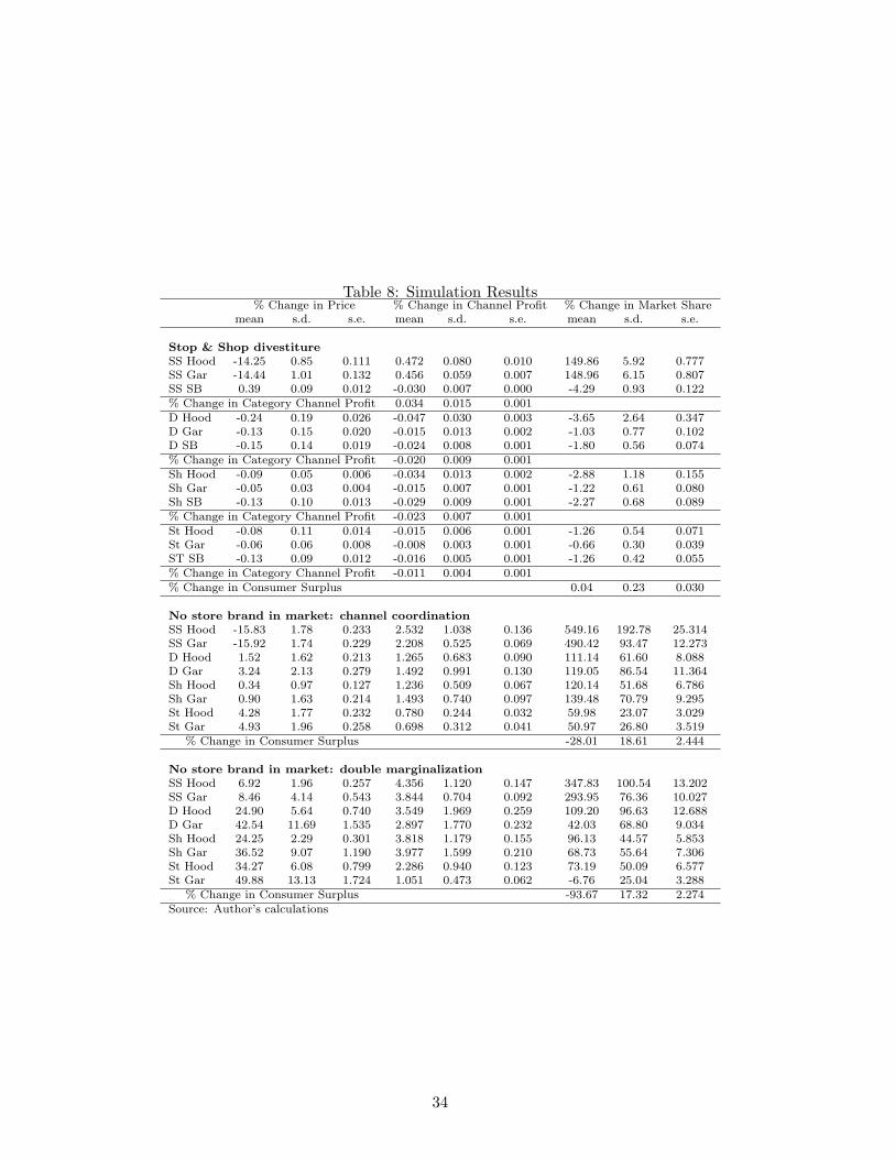
Table 8: Simulation Results% Change in Price % Change in Channel Profit % Change in Market Share

mean s.d. s.e. mean s.d. s.e. mean s.d. s.e.

Stop & Shop divestitureSS Hood -14.25 0.85 0.111 0.472 0.080 0.010 149.86 5.92 0.777SS Gar -14.44 1.01 0.132 0.456 0.059 0.007 148.96 6.15 0.807SS SB 0.39 0.09 0.012 -0.030 0.007 0.000 -4.29 0.93 0.122% Change in Category Channel Profit 0.034 0.015 0.001D Hood -0.24 0.19 0.026 -0.047 0.030 0.003 -3.65 2.64 0.347D Gar -0.13 0.15 0.020 -0.015 0.013 0.002 -1.03 0.77 0.102D SB -0.15 0.14 0.019 -0.024 0.008 0.001 -1.80 0.56 0.074% Change in Category Channel Profit -0.020 0.009 0.001Sh Hood -0.09 0.05 0.006 -0.034 0.013 0.002 -2.88 1.18 0.155Sh Gar -0.05 0.03 0.004 -0.015 0.007 0.001 -1.22 0.61 0.080Sh SB -0.13 0.10 0.013 -0.029 0.009 0.001 -2.27 0.68 0.089% Change in Category Channel Profit -0.023 0.007 0.001St Hood -0.08 0.11 0.014 -0.015 0.006 0.001 -1.26 0.54 0.071St Gar -0.06 0.06 0.008 -0.008 0.003 0.001 -0.66 0.30 0.039ST SB -0.13 0.09 0.012 -0.016 0.005 0.001 -1.26 0.42 0.055% Change in Category Channel Profit -0.011 0.004 0.001% Change in Consumer Surplus 0.04 0.23 0.030

No store brand in market: channel coordinationSS Hood -15.83 1.78 0.233 2.532 1.038 0.136 549.16 192.78 25.314SS Gar -15.92 1.74 0.229 2.208 0.525 0.069 490.42 93.47 12.273D Hood 1.52 1.62 0.213 1.265 0.683 0.090 111.14 61.60 8.088D Gar 3.24 2.13 0.279 1.492 0.991 0.130 119.05 86.54 11.364Sh Hood 0.34 0.97 0.127 1.236 0.509 0.067 120.14 51.68 6.786Sh Gar 0.90 1.63 0.214 1.493 0.740 0.097 139.48 70.79 9.295St Hood 4.28 1.77 0.232 0.780 0.244 0.032 59.98 23.07 3.029St Gar 4.93 1.96 0.258 0.698 0.312 0.041 50.97 26.80 3.519

% Change in Consumer Surplus -28.01 18.61 2.444

No store brand in market: double marginalizationSS Hood 6.92 1.96 0.257 4.356 1.120 0.147 347.83 100.54 13.202SS Gar 8.46 4.14 0.543 3.844 0.704 0.092 293.95 76.36 10.027D Hood 24.90 5.64 0.740 3.549 1.969 0.259 109.20 96.63 12.688D Gar 42.54 11.69 1.535 2.897 1.770 0.232 42.03 68.80 9.034Sh Hood 24.25 2.29 0.301 3.818 1.179 0.155 96.13 44.57 5.853Sh Gar 36.52 9.07 1.190 3.977 1.599 0.210 68.73 55.64 7.306St Hood 34.27 6.08 0.799 2.286 0.940 0.123 73.19 50.09 6.577St Gar 49.88 13.13 1.724 1.051 0.473 0.062 -6.76 25.04 3.288

% Change in Consumer Surplus -93.67 17.32 2.274Source: Author’s calculations

34

FOOD MARKETING POLICY CENTER RESEARCH REPORT SERIES

This series includes final reports for contract research conducted by Policy Center Staff. The series also contains research direction and policy analysis papers. Some of these reports have been commissioned by the Center and are authored by especially qualified individuals from other institutions. (A list of previous reports in the series is available on our web site.) Other publications distributed by the Policy Center are the Working Paper Series, Journal Reprint Series for Regional Research Project NE-165: Private Strategies, Public Policies, and Food System Performance, and the Food Marketing Issue Paper Series. Food Marketing Policy Center staff contribute to these series. Individuals may receive a list of publications in these series and paper copies of older Research Reports are available for $20.00 each, $5.00 for students. Call or mail your request at the number or address below. Please make all checks payable to the University of Connecticut. Research Reports can be downloaded free of charge from our web site given below.

Food Marketing Policy Center 1376 Storrs Road, Unit 4021

University of Connecticut Storrs, CT 06269-4021

Tel: (860) 486-1927

FAX: (860) 486-2461 email: fmpc@uconn.edu

http://www.fmpc.uconn.edu