determining the effects of climate change and market
TRANSCRIPT
Journal of Agricultural Sciences (Tarim Bilimleri Dergisi) 2021, 27 (2) : 204 - 210 DOI: 10.15832/ankutbd.495246
Journal of Agricultural Sciences (Tarim Bilimleri Dergisi)
J Agr Sci-Tarim Bili e-ISSN: 2148-9297
jas.ankara.edu.tr
Determining the Effects of Climate Change and Market Prices on Farm’s Structure
by Using an Agent Based Model
Hooman MANSOORİa , Mohammad GHORBANİa* , Mohammad Reza KOHANSALa
aDepartment of Agricultural Economics, Agricultural College, Ferdowsi University of Mashhad, Mashhad, IRAN
ARTICLE INFO Research Article
Corresponding Author: Mohammad GHORBANİ, E-mail: [email protected]
Received: 11 December 2018 / Revised: 21 December 2019 / Accepted: 07 February 2020 / Online: 31 May 2021
ABSTRACT In this study, an agent-based model was used to simulate structure change
of farms during 20 years period of climate and market price changes in
the rural area of Eslamshahr City in Iran. Decision rules that used in the
model are based on the information that collected by direct interviews
with farmers. So the model includes rules that define the relationship
between agents and their environment. Results clearly showed that
farmers' behavior patterns and the cover of agricultural land in the region
affected by environmental and market factors changes. Comparison of the
results of model implementation for various scenarios has shown that the
highest yield and income loss has occurred in scenarios where there was
a 10% reduction in access to water. Also, there is a less decrease in the
crops land size in groups which includes small and medium farmers.
Keywords: Agent based, Climate, Farm Structure, Land use, Iran
© Ankara University, Faculty of Agriculture
1. Introduction
The social, economic and spatial dynamics of rural regions are often affected by the processes and dynamics of the agricultural
farm structure changes. These dynamics are complex processes caused by the interaction between natural and social systems at
different scales. The role that a farm takes within this complex process depends not only on the farm's characteristics, the
characteristics of the farmer or farm manager but also on local competition, as well as the economic, institutional and
environmental conditions. For an adequate understanding of the underlying processes, it is important to capture not only the
interactions amongst and between farms and their environment but also the farms' behavior, and their decision processes (Appel
& Balmann 2018).
The ongoing internal and external pressure on farmers has resulted in the fluctuation of gross margins, income, and a
continuous change in the number of farmers in the region. Understanding these significant trends and their impact on the farm
structure requires a deeper knowledge of the mechanisms involved and the impacts of different policy measures (Beckers et al.
2018). The core theme of agriculture structural change science is to understand the dynamics of the farmer's decision-making
rules according to these trends (Schindler 2009). As mentioned above, the driving forces can be categorized as endogenous and
exogenous processes of a region. Endogenous processes are socio-economic and biophysical conditions of farms in a specific
region including farmer’s experience, preferences, economic condition, and land fertility. Exogenous processes are those
occurring at global, national and regional scales, varying from changes in the market prices to climate change and policy
frameworks (Valbuena et al. 2010).
Agriculture is one of the most climate-sensitive sectors and directly affected by changes in climate conditions. Farmers may
implement climate change adaptation measures to reduce or avoid adverse developments and take advantage of emerging
opportunities. Others may forbear to adapt which results in a lack of timely adaptation. On the other hand, the volatility and price
imbalance of agricultural products and inputs as an exogenous factor influences farmer's income and expenditure situation and,
consequently, the welfare of their lives. The change in farmers' welfare status will shape the decision-making process and the
selection of activity options in the upcoming period. Farmers’ adaptation decisions -such as other human behavior- is influenced
by the individual characteristics and economic and social conditions of the farmer (Mitter et al. 2019). Agriculture in Iran is also
affected by market prices and climatic conditions, which can lead to changes in farmer preferences and behavior, and change in
agricultural cover and economic outcomes in the region. Iran is one of the world’s water-scarce regions and is extremely
vulnerable to the impacts of climate change due to its high dependency on climate-sensitive agriculture (Karimi et al. 2017). A
new approach to analyze and simulate farm structural changes according to exogenous and endogenous factors is the use of
agent-based simulation models. Behavioural or ‘process-based' models such as agent-based models (ABMs) have received
Mansoori et al. - Journal of Agricultural Sciences (Tarım Bilimleri Dergisi), 2021, 27(2): 204-210
205
increasing attention because they allow the simulation of emergent social and economic conditions from underlying external
factors such as climate changes and market prices fluctuations and internal factors like behavioral processes of farmer’s decision
making and land use changes (Seo et al. 2018). Hailegiorgis et al. (2018), used an agent-based model to find the impact of climate
change on the adaptive capacity of rural communities in Ethiopia and showed that climate effects caused farmers to migrate from
the region. Lamperti et al. (2017) introduced an agent-based model to assess and monitor the Coupled Climate and Economic
Dynamics. Wossen et al. (2017) provided an ex-ante assessment of the impacts of climate and price variability on household
income and food security in Ethiopia and Ghana.
The ABM model in this research includes a socio-ecological system representing the farm region of "Eslamashahr" in Iran
that is informed by empirical data from a social survey about the behavior and heterogeneity of farmers. This area covers 4 rural
main districts and 49 villages. The dominate cultivation crops are wheat, barley, corn, and alfalfa. According to Iran’s third
national report to UNFCC (The United Nations Framework Convention on Climate Change, 2017), the projections of mean
temperature based on scenarios for Iran show that the mean temperature will increase in the whole country in future decades
compared to the baseline period. So, the temperature is estimated to increase up to 1 degree in some parts of the country that the
current study was conducted. Also, precipitation changes in the area will be up to -4.4%. Meanwhile, according to the data
provided by the statistics of the Ministry of Agriculture and Statistics of Iran in different years, farmers in this region like other
parts of the country face annual changes in prices of products and production costs, as in recent years, the average prices of
agricultural products has grown 9.66%, and the average annual cost of production has grown by 13.08%. Therefore, the purpose
of this study is to understand how the interaction between agents or farmers in agricultural land with climate change in the region
and market fluctuations, and to simulate and measure the economic outcomes of this interaction for 20 years. Whilst ABM is
increasingly applied to assess farm structural changes in several regions and countries but to our knowledge, no similar agent-
based studies have been so far conducted in Iran.
2. Material and Methods
This research adopted an agent-based model as a suitable approach to quantify the agricultural systems, their structural change,
and endogenous adjustment to climate changes and price volatilities in “Eslamshahr” as an example of a traditional agricultural
landscape during a period of 20 years from 2016 to 2036. The model was constructed using the NetLogo software. The framework
of this model and the type of variables for entry into the simulation model Were determined after the review of previous similar
studies (Lobanco & Esposti 2010; Bert et al. 2011; Lamperti et al. 2017) and according to the conditions of the farmers in the
region. Farmers' economic and social heterogeneity and their differences in reaction thresholds to external factors lead to their
different outcomes in a given period. Here, quantitative models based on aggregated data can’t meet the research needs but in
agent-based framework, the model is implemented for every individual agent and ultimately the overall agricultural region profile
can be simulated. Information was collected from interviews with farmers and agricultural administrators. The environment,
which influences farmer’s decisions, is defined based on economic and climatic parameters. The economic parameters include
product prices and costs of production such as fertilizers, pesticides, labor, and land costs (i.e. rental price). The climatic
parameters are represented by the effects of temperature and rainfall on yields. Considering the diversity of farm sizes in the
county, a stratified sampling method was selected with proportional allocation. The sample size was 195 (out of 585 households)
and the variables used in the research model are defined in Table 1:
Table 1- Variables used in agent based model
Description Variable
Gross income of each crop per hectare (Tomans) 𝐺𝐼𝑗,𝑡 = 𝑃𝑗,𝑡 ∗ 𝑌𝑗,𝑡
Land size of crop J (hectares) 𝐶𝐿𝐽
Total farm land size (hectares) 𝑇𝐶𝐿𝑡 = ∑ 𝐶𝐿𝑗,𝑡
Total farm gross income (Tomans) 𝑇𝐺𝐼𝑡 = ∑(𝐺𝐼𝑗,𝑡 ∗ 𝐶𝐿𝑗,𝑡)
Total farm costs (Tomans) 𝑇𝐸𝑋𝑃𝑡 = ∑(𝐸𝑋𝑃𝑗,𝑡 ∗ 𝐶𝐿𝑗,𝑡)
Total farm net income (Tomans) 𝑇𝑁𝐼𝑡 = 𝑇𝐺𝐼𝑡 − 𝑇𝐸𝑋𝑃𝑡
Net income per hectare (Tomans) 𝑁𝐼𝑡 = 𝑇𝑁𝐼𝑡/𝑇𝐶𝐿𝑡
Total farm labor (man 𝐿𝐴𝐵𝑂𝑅𝑡 = ∑ (𝐿𝐴𝐵𝑂𝑅𝑗,𝑡 ∗ 𝐶𝐿𝑗,𝑡)𝑗
Aspiration level or expected income per hectare (Tomans) 𝐴𝐿𝑡
Opportunity cost of a period of use of each hectare (Tomans) 𝑂𝐶 = 𝑅𝑃𝑡 + 𝐼𝑅𝑡
Average value of rent per hectare of farm land in the region (Tomans) 𝑅𝑃𝑡
Interest amount (interest rate=0.15), (Tomans) 𝐼𝑅𝑡 = 0.15 ∗ (𝑅𝑃𝑡 + 𝐸𝑋𝑃𝑡)
Working capital (Tomans) 𝑊𝐶𝑡 = 𝑇𝑁𝐼𝑡 − 𝑆𝐼𝑁𝐶𝑡 + 𝑇𝑅𝐼𝑡 − 𝑇𝑅𝐸𝑡 + 𝑊𝐶𝑡−1
Maximum land that farmer can lease in the next period potentially 𝑁𝐿 = [𝑊𝐶/𝑅𝑃] Farmer's Household Livestock Minimum Cost (Tomans) 𝑆𝐼𝑁𝐶𝑡
Total revenue from land rent out (Tomans) 𝑇𝑅𝐼𝑡 = 𝑅𝑃𝑡 . 𝑅𝐶𝐿𝑡
Total cost of leasing farm land (Tomans) 𝑇𝑅𝐸𝑡 = 𝑅𝑃𝑡 . 𝐿𝐶𝐿𝑡
The amount of land rented out (hectares) 𝑅𝐶𝐿𝑡 The amount of land leased (hectares) 𝐿𝐶𝐿𝑡
Mansoori et al. - Journal of Agricultural Sciences (Tarım Bilimleri Dergisi), 2021, 27(2): 204-210
206
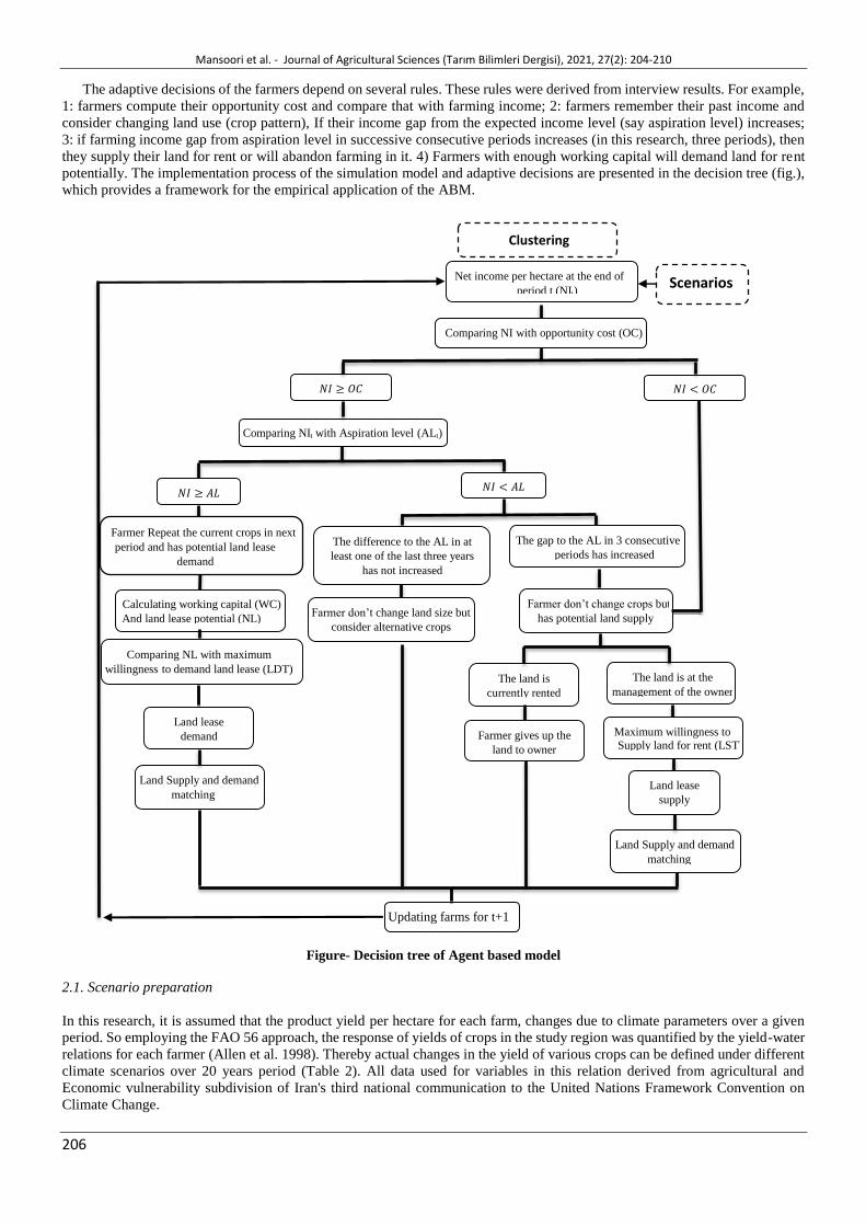
The adaptive decisions of the farmers depend on several rules. These rules were derived from interview results. For example,
1: farmers compute their opportunity cost and compare that with farming income; 2: farmers remember their past income and
consider changing land use (crop pattern), If their income gap from the expected income level (say aspiration level) increases;
3: if farming income gap from aspiration level in successive consecutive periods increases (in this research, three periods), then
they supply their land for rent or will abandon farming in it. 4) Farmers with enough working capital will demand land for rent
potentially. The implementation process of the simulation model and adaptive decisions are presented in the decision tree (fig.),
which provides a framework for the empirical application of the ABM.
Figure- Decision tree of Agent based model
2.1. Scenario preparation
In this research, it is assumed that the product yield per hectare for each farm, changes due to climate parameters over a given
period. So employing the FAO 56 approach, the response of yields of crops in the study region was quantified by the yield-water
relations for each farmer (Allen et al. 1998). Thereby actual changes in the yield of various crops can be defined under different
climate scenarios over 20 years period (Table 2). All data used for variables in this relation derived from agricultural and
Economic vulnerability subdivision of Iran's third national communication to the United Nations Framework Convention on
Climate Change.
Clustering
Land Supply and demand
matching
Updating farms for t+1
Net income per hectare at the end of
period t (NIt)
Scenarios
Comparing NI with opportunity cost (OC)
𝑁𝐼 ≥ 𝑂𝐶
𝑁𝐼 < 𝑂𝐶
𝑁𝐼 ≥ 𝐴𝐿
𝑁𝐼 < 𝐴𝐿
Comparing NIt with Aspiration level (ALt)
Calculating working capital (WC)
And land lease potential (NL)
Land lease
demand
The difference to the AL in at
least one of the last three years
has not increased
Farmer Repeat the current crops in next
period and has potential land lease
demand
The gap to the AL in 3 consecutive
periods has increased
Farmer don’t change land size but
consider alternative crops
Farmer don’t change crops but
has potential land supply
Comparing NL with maximum
willingness to demand land lease (LDT) The land is
currently rented The land is at the
management of the owner
Farmer gives up the
land to owner Maximum willingness to
Supply land for rent (LST)
Land lease
supply
Land Supply and demand
matching

Mansoori et al. - Journal of Agricultural Sciences (Tarım Bilimleri Dergisi), 2021, 27(2): 204-210
207
Table 2- Climate change pre-scenarios
- Percentage of change in annual rainfall: -4.4%
- Percentage of change in annual temperature: +1%
Annual Change of yields (𝛼) Condition
alfalfa maize barley wheat
-0.17% -3.16% -0.27% -0.3% Fixing access to water as much as the base year A1
-0.64% -0.88% -0.8% -0.79% Reducing 10% of access to water A2
Notes: -In scenario A1 it is assumed that, despite the decrease in rainfall over a period of time, using improved technology, through proper irrigation, the
available water is fixed at the base year and main reason of yield decrease is changing climate and crop evapotranspiration, -In scenario A2 it is assumed that the total amount of available water for agriculture will decrease by 10% at the end of the simulation period
In this research, two pre-scenarios are defined about predicted changes in products prices and production cost.
Table 3- Price changes pre-scenarios
Annual growth rate of
production costs
Annual growth rate of
product price Pre-scenarios
+13.86% +9.66% Growth rate of production costs ≥ growth rate of product prices B1
+13.86% +13.86% Growth rate of production costs = growth rate of product prices B2
Notes: - In scenario B1, it is assumed that production costs and prices of the products are the same as the past 15 years (annual change of products prices= +9.66% and annual change of production costs = +13.86%), -In scenario B2, production costs and product prices grow by as much as 13.86 percent.
Based on the above pre-scenarios, the following mixed scenarios are presented:
A1B1: fixed water access as much as the base year + continued trend over the last 15 years in rising product prices and
production costs
A1B2: fixed water access as much as the base year + similar changes in product prices and production costs
A2B1: 10% reduction in water access + continued trend over the last 15 years in rising product prices and production costs
A2B2: 10% reduction in water access + similar changes in product prices and production costs
2.2. Economic calculations
This submodel calculates the economic results for a farmer during one full production cycle. After preparing scenarios, by using
variables such as total production costs (TEXP), product prices (Pj), yield per hectare (Yj), total gross income (TGI), gross
income per hectare (GI), and net income in each hectare (NI) would be calculated at the end of each period t.
Variables that directly would be affected by scenarios include:
𝑌𝑗,𝑡 = 𝑌𝑗,0 ∗ (1 + 𝛼)𝑡: Yield in a hectare of product j in year t
𝑃𝑗,𝑡 = 𝑃𝑗,0 ∗ (1 + 𝛽)𝑡 : Market price of product j in year t
𝐸𝑋𝑃𝑗,𝑡 = 𝐸𝑋𝑃𝑗,0 ∗ (1 + 𝛽)𝑡: Production cost in a hectare of product j in year t
A part of the results of the submodel is the financial balance for a farmer and his/her household at the end of a cycle. The
balance is expressed as the working capital accumulated by an agent at the end of the cycle (WC). Briefly, the accumulation of
working capital is the result of the balance between available capitals from previous cycles, received total income, and incurred
total expenses during a production cycle. After calculating the net income per hectare (NI), the farmer calculates the opportunity
cost of the agricultural activity (OC) and compares it with the NI. If the net income of each hectare is greater than or equal to the
cost of opportunity, then the farmer will compare the net incomes per hectare (NI) with the expected value or Aspiration level
(ALt) (Bert et al. 2011). The aspiration level would be calculated by average income per hectares of successful farmers in the
region. It is assumed that farmers with the highest technical efficiency are successful farmers. For this purpose, the technical
efficiency coefficient of all farms was calculated by the DEA1 method and the average of NI for farmers in each cluster with an
efficiency coefficient above 0.8 determined as aspiration level in that cluster. Now, if the net income is less than the aspiration
level, then the process of changing the gap or the difference with this threshold will be the benchmark for the decision. If this
gap increases for three consecutive years, the farmer will have a potential supply of land.
(𝑁𝐼𝑡/𝐴𝐿𝑡) > (𝑁𝐼𝑡−1/ 𝐴𝐿𝑡−1) > (𝑁𝐼𝑡−2/𝐴𝐿𝑡−2) (2)
1 Data envelopment analysis

Mansoori et al. - Journal of Agricultural Sciences (Tarım Bilimleri Dergisi), 2021, 27(2): 204-210
208
If the net income per hectare is less than the expected value, but the difference does not increase for all three consecutive
years, the farmer will only seek to replace the crops according to crop preferences. So he will choose crops for the next year
from a discrete set of available options. For this purpose, crop preferences were determined by performing an interview with
farmers and utility values obtained for each crop according to their statements. If the land is rented, it will be transferred to the
owner and if the land is a property, then the land offered for rent is equivalent to the maximum willingness to rent out (LST),
that previously obtained by interviewing each farmer. If NI ≥ AL, the current period cropping pattern will be repeated in the next
period and the farmer will have a potential land lease demand. For farmers who have a potential land lease demand, at first the
working capital (WC) will be calculated and then the maximum land that farmers can lease (NL) will be determined (Bert et al.
2011). Comparing (NL) with the maximum willingness to lease land (LDT) determines the actual demand for land lease. If NL
≥ LDT then actual demand is equal to LDT and if NL < LDT then it is equal to NL.
3. Results and Discussion
Before running the simulation model, farmers were divided into three classes to obtain different classes proportional to the size
and scale of production, using K-Means clustering method. In this method, every data point is allocated to each of the clusters
through reducing the in-cluster sum of squares. In other words, the K-means algorithm identifies k number of centroids, and then
allocates every data point to the nearest cluster, while keeping the centroids as small as possible. So, Cluster 1 with 105 farmers,
cluster 2 with 378 farmers and cluster 3 with 378 farmers were identified.
3.1. Simulation model results
The results show that in A1B1 scenario the total cropping land size in cluster 2 and cluster 1 have the highest decrease at the end
of the simulation period. Large-scale farmers are more flexible while reducing economic benefits due to increased production
costs (in this scenario, the rate of increase in production costs is higher than the rate of increase in prices of products), but smaller
farmers with lower income earnings respond quicker. According to the model decision tree, which compares net income per
hectare with the opportunity cost and also net income per hectare with expected income (Aspiration level) over consecutive
periods, a larger percentage of small farmers Due to the lack of desirability, reduced their cultivated land or stop cultivating to
use the released capital in other businesses. Comparison of yield changes per hectare of the products indicated that the highest
yield loss was due to the wheat product, which is reduced by 5.8%, and in all three clusters this reduction value is the same. The
yield of barley and alfalfa products in cluster 3, which includes large-scale farmers, has declined less. It seems that farmers have
been able to compensate for the decline in yields due to climate change, given access to more machinery and equipment and the
use of agronomic methods.
Table 4- Simulation results for A1B1 scenario
Cluster 3 Cluster 2 Cluster 1
Change
percent A0B0 A1B1
Change
percent A0B0 A1B1
Change
percent A0B0 A1B1
-2.1 4989 4884 -7.5 1275 1179 -6.8 327 304.5 Total cropping land size (hectares)
-5.8 5220 4915 -5.8 4275 4025 -5.8 3877 3651 Yield in hectare of wheat (kg)
-4.8 5071 4823 -5.2 3926 3719 -5.2 3833 3631 Yield in hectare of barley (kg)
-3.1 52000 50355 -3.1 44288 42892 -1.07 40800 40363 Yield in hectare of maize (kg)
-3.05 14579 14134 -3.3 14100 13628 -3.35 14000 13531 Yield in hectare of alfalfa (kg)
-47.3 3.8 2 -45.3 2.98 1.58 -43.3 2.72 1.54 Income/cost index
-0.86 2076 2058 -7.8 152 140 -9.9 151 136 Average labor work in each farm
(labors*Days)
To compare the economic indicators of farmers in three clusters, the ratio of total income to total cost is used. As can be seen,
the value of this index in cluster 3 is higher than the other two clusters. The lowest employment reduction rate is for cluster 3
farmers, which was only 0.86% lower than the beginning of the period.
In A1B2 scenario, total cropping land size in the cluster 2 has the highest decrease. The highest yield in hectare loss is due
to wheat production, which is reduced by 5.8%, and in all three clusters this reduction is similar. The value of the income/expense
ratio in cluster 2 and 3 is higher than cluster 1.
In the A2B1 scenario, it is assumed that the total water consumption of crops will decrease by 10%. As a result, the yield loss
is not only due to an increase in evapotranspiration but also a reduction in water availability. On the other hand, in this scenario,
it is assumed that the changes in annual product prices and production costs are the same as in the last 15 years, with the price
of products rising by 9.66% annually and production costs by 13.068%. Comparison of yield changes per hectare of the products

Mansoori et al. - Journal of Agricultural Sciences (Tarım Bilimleri Dergisi), 2021, 27(2): 204-210
209
showed that the highest yield loss was related to alfalfa. The value of the ratio of income to expense at the end of the simulation
period in cluster 2 and 3 is higher than cluster 1. Table 5- Simulation results for A1B2 scenario
Cluster 3 Cluster 2 Cluster 1
Variable Change
percent A0B0 A1B1
Change
percent A0B0 A1B1
Change
percent A0B0 A1B1
-2.2 4989 4878 -4.2 1275 1221 -1.8 327 321 Total cropping land size (hectares)
-5.8 5220 4915 -5.8 4275 4025 -5.8 3877 3651 Yield in hectare of wheat (kg)
-4.8 5071 4823 -5.2 3926 3719 -5.2 3833 3631 Yield in hectare of barley (kg)
-3.1 52000 50355 -3.1 44288 42892 -1.07 40800 40363 Yield in hectare of maize (kg)
-3.05 14579 14134 -3.3 14100 13628 -3.3 14000 13532 Yield in hectare of alfalfa (kg)
-2.6 3.8 3.7 -2.6 2.98 2.9 3.3 2.72 2.81 Income/cost index
-0.86 2076 2058 -4.6 152 145 -4.6 151 144 Average labor work in each farm
(labors*Days)
Table 6- Simulation results for A2B1 scenario
Cluster 3 Cluster 2 Cluster 1
Variable Change
percent A0B0 A1B1
Change
percent A0B0 A1B1
Change
percent A0B0 A1B1
-4.3 4989 4774 -4.07 1275 1223 -20.7 327 259 Total cropping land size (hectares)
-14.6 5220 4454 -14.6 4275 3647 -14.6 3877 3309 Yield in hectare of wheat (kg)
-14.4 5071 4336 -14.8 3926 3343 -14.8 3833 3264 Yield in hectare of barley (kg)
-16.2 52000 43569 -16.2 44288 37111 -14.4 40800 34924 Yield in hectare of maize (kg)
-11.7 14579 12861 -12.05 14100 12400 -12.05 14000 12313 Yield in hectare of alfalfa (kg)
-53.42 3.8 1.77 -53.42 2.98 1.39 -49.6 2.72 1.37 Income/cost index
-2.89 2076 2016 -5.2 152 144 -22.5 151 117 Average labor work in each farm
(labors*Days)
In the A2B2 scenario, as in the previous, a 10% reduction in water availability will exacerbate this decline in yields. Also,
the annual price changes of products and production costs are the same and grow as much as 13.68% annually. Results showed
that total cropping land size of the area in cluster 2 and cluster 1 have the greatest decrease.
Table 7- Simulation results for A2B2 scenario
Cluster 3 Cluster 2 Cluster 1
Variable Change
percent A0B0 A1B1
Change
percent A0B0 A1B1
Change
percent A0B0 A1B1
-2.3 4989 4872 -4.7 1275 1214 -10.09 327 294 Total cropping land size (hectares)
-14.6 5220 4454 -14.6 4275 3647 -14.6 3877 2308 Yield in hectare of wheat (kg)
-14.4 5071 4336 -14.8 3926 3343 -14.8 3833 3264 Yield in hectare of barley (kg)
-16.2 52000 43569 -16.2 44288 37111 -14.4 40800 34924 Yield in hectare of maize (kg)
-11.7 14579 12861 -12.05 14100 12400 -12.05 14000 12312 Yield in hectare of alfalfa (kg)
-13.4 3.8 3.29 -13.4 2.98 2.58 -7.72 2.72 2.51 Income/cost index
-1.01 2076 2055 -5.9 152 143 -12.5 151 132 Average labor work in each farm
(labors*Days)
4. Conclusions
In this research, the results of the implementation of the agent-based simulation model to study farm structural changes in the
rural area of “Eslamshahr” for 20 years are presented in detail. The simulation results clearly showed that farmers' behavior
patterns and the agricultural land cover affected by environmental and market factors variation. This is consistent with numerous
studies related to the underlying agent-based simulation (Lobianco & Esposti 2010; Bert et al. 2011; Acosta et al. 2014; Lamperti
et al. 2017; Wossen et al. 2017, Seo et al. 2018). Results also suggested that the preferences and subjective priorities of each
farmer in determining the cropping pattern and selection of products have a significant effect on the final agricultural cover in
the region, which is similar to the results of Valbuena et al. (2010). Results indicated that at the end of the simulation period, due
to climate change, water scarcity and the change of the prices of products and production costs, the number of active agricultural
farms in the cluster 1, which includes small-scale farmers, will be further reduced. Also, the employment in the agricultural
sector across all scenarios and the total cropping land size in the number of scenarios will decrease. Such a decrease intensifies
under the scenario of a 10 percent reduction in water access and the continuation of the past trend in the annual change in prices
and production costs (A2B1). In scenario A2B1 and A2B2, where the 10% reduction in access to water occurs during the
simulation period, there is the highest yield loss, for example, wheat yields fall by more than 14% in cluster 3. This has resulted

Mansoori et al. - Journal of Agricultural Sciences (Tarım Bilimleri Dergisi), 2021, 27(2): 204-210
210
in numerous consequences such as declining production and employment, changing the dominant agricultural profile in the
region, and increasing the likelihood of land use change. It is essential to create adequate incentives for farmers by the
government to compensate for the adverse effects of possible scenarios and encouraging the development of modern agricultural
practices to reduce the functional effects of climate change and the lack of access to water.
Encouraging the development of products that demonstrate greater flexibility and adaptation to climate change can be one of
the suggested strategies. The promotion and training of modern agricultural practices and the provision of mechanization needed
by farmers in the region will help to improve the performance of agricultural farms. The highest drop in employment was
observed in small and medium-size agricultural units. There is also the highest income/cost ratio in large agricultural units.
Appropriate policies and support orientation towards small and medium-size farms are necessary to increase competitiveness
and sustainability in situations where production performance is reduced in the simulation horizon. In a situation where in the
coming years, small scale farms will have a more economic vulnerability to climate change and market fluctuations, encouraging
the creation and development of production cooperatives in the region with the participation of small-scale farms can lead to
increased productivity and reduced costs.
References
Acosta L, Rounsevell M, Bakker M, Van Doorn A, Montserrat G & Delgado M (2014). An agent-based assessment of land use and ecosystem
changes in the traditional agricultural landscape of Portugal. Journal of Intelligent Information Management 6(2):55-
80 https://doi.org/10.4236/iim.2014.62008
Allen R, Pereira L S, Raes D & Smith M (1998). Crop evapotranspiration, Guidelines for computing crop water requirements. FAO Irrigation
and drainage, paper 56, Food and Agriculture Organization of the United Nations
Appel F & Balmann A (2018). Human behavior versus optimizing agents and the resilience of farms-Insights from agent-based participatory
experiments with Farm AgriPoliS. Ecplogical Complexity 40(100731) https://doi.org/10.1016/j.ecocom.2018.08.005
Beckers V, Beckers J, Vanmaecke M & Van Hecke, E (2018). Modelling farm growth and its impact on Agricultural land use: A country scale
application of an agent-based model. Journal of Land 7(3): 109 https://doi.org/10.3390/land7030109
Bert F, Podesta P, Rovere S & Menendez A (2011). An agent-based model to simulate structural and land-use changes in agricultural systems
of the Argentine pampas. Journal of Ecological Modelling 22(19): 3486-3499 https://doi.org/10.1016/j.ecolmodel.2011.08.007
Hailegiorgis A, Crooks A & Cioffi-Revilla C (2018) An agent-based model of rural households’ adaptation to climate change. Journal of
Artificial Societies and Social Simulation 21(4): 4 https://doi.org/10.18564/jasss.3812
UNFCC (2017). Iran’s third national report, National climate change office at the department of environment on behalf of the government of
the Islamic Republic of Iran
Karimi V, Karami E & Keshavarz M (2017). Climate change and agriculture: Impacts and adaptive responses in Iran. Journal of Integrative
Agriculture 17(1): 1-15 https://doi.org/10.1016/s2095-3119(17)61794-5
Lamperti F, Dosi G, Napoletano M, Roventini A & Sapio A (2017). Faraway, so close: Coupled climate and economic dynamics in an agent-
based integrated assessment model. Journal of Ecological Economics 150: 315-339 https://doi.org/10.2139/ssrn.2944328
Lobianco A & Esposti R (2010). The regional multi-agent simulator (RegMAS): An open-source spatially explicit model to assess the impact
of agricultural policies. Journal of Computers and Electronics in Agriculture 72(1): 14-26 https://doi.org/10.1016/j.compag.2010.02.006
Mitter H, Larcher M, Schonhart M, Stottinger M & Schmid E (2019). Exploring farmers’ climate change perceptions and adaptation intentions:
Empirical evidence from Austria. Journal of Environmental management 63(6): 804-821 https://doi.org/10.1007/s00267-019-01158-7
Schindler J (2009). A multi-agent system for simulating land-use and land-cover change in the Atankwidi catchment of Upper East Ghana.
Unpublished PhD thesis, Faculty of mathematics and natural sciences, University of Bonn, Germany
http://hdl.handle.net/20.500.11811/4160
Seo B, Crown C, Rounsevell M (2018). Evaluation and calibration of an agent based land use model using remotely sensed land cover and
primary productivity data. In: proceedings of the IEEE International Geoscience and Remote Sensing Symposium, 22-27 July, Valencia,
Spain https://doi.org/10.1109/igarss.2018.8518023
Valbuena D, Verbung P H, Bregt A & Lightenberg A (2010). An agent-based approach to model land-use change at a regional scale. Journal
of Landscape Ecology 25(2): 185-199 https://doi.org/10.1007/s10980-009-9380-6
Wossen T, Berger T, Mekbib G H & Troost C (2017). Impacts of climate variability and food price volatility on household income and food
security of farm households in East and West Africa. Journal of Agricultural systems 163: 7-15 https://doi.org/10.1016/j.agsy.2017.02.006
© 2021 by the authors. Licensee Ankara University, Faculty of Agriculture, Ankara, Turkey. This article is an open access article distributed under the terms and conditions of the Creative Commons Attribution (CC BY) license (http://creativecommons.org/licenses/by/4.0/).