determining shallow aquifer vulnerability by the drastic

J. Earth Syst. Sci. (2017) 126:89 c© Indian Academy of SciencesDOI 10.1007/s12040-017-0870-7

Determining shallow aquifer vulnerability bythe DRASTIC model and hydrochemistryin granitic terrain, southern India

N C Mondal1,∗, S Adike2, V S Singh1, S Ahmed1 and K V Jayakumar3

1Earth Process Modeling Group, CSIR-National Geophysical Research Institute, Hyderabad 500 007, India.2Rural Water Supply & Sanitation, Mahaboobnagar, Telangana, India.3Water & Environmental Division, Department of Civil Engineering, National Institute of Technology,Warangal 506 004, India.*Corresponding author. e-mail: [email protected]

Received: 28 October 2016 / Revised: 20 January 2017 / Accepted: 15 March 2017 /Published online: 2 September 2017

Shallow aquifer vulnerability has been assessed using GIS-based DRASTIC model by incorporating themajor geological and hydrogeological factors that affect and control the groundwater contaminationin a granitic terrain. It provides a relative indication of aquifer vulnerability to the contamination.Further, it has been cross-verified with hydrochemical signatures such as total dissolved solids(TDS), Cl−, HCO−

3 , SO2−4 and Cl−/HCO−

3 molar ratios. The results show four zones of aquifervulnerability (i.e., negligible, low, moderate and high) based on the variation of DRASTIC VulnerabilityIndex (DVI) between 39 and 132. About 57% area in the central part is found moderately andhighly contaminated due to the 80 functional tannery disposals and is more prone to groundwateraquifer vulnerability. The high range values of TDS (2304–39,100 mg/l); Na+(239– 6,046 mg/l)and Cl− (532–13,652 mg/l) are well correlated with the observed high vulnerable zones. The valuesof Cl−/HCO−

3 (molar ratios: 1.4–106.8) in the high vulnerable zone obviously indicate deteriorationof the aquifer due to contamination. Further cumulative probability distributions of these parametersindicate several threshold values which are able to demarcate the diverse vulnerability zones ingranitic terrain.

Keywords. Shallow aquifers; DRASTIC model; hydrochemical signatures; vulnerability assessment;granitic terrain; southern India.

1. Introduction

The aquifer vulnerability has been defined usingDRASTIC model (Albinet and Margat 1970; Alleret al. 1987). The word ‘DRASTIC’ is an acronymabbreviated for seven parameters such as depth ofwater table (D), net recharge (R), aquifer media(A), soil media (S), topography (T), impact of

vadose zone (I) and hydraulic conductivity (C).It is the measure of possibility of pollution orcontamination at the ground level to reach anaquifer. Numerous schemes have been developedfor assessing vulnerability. The DRASTIC mod-eling is preferred among many other techniquesas it has the capacity to show all hydrogeolog-ical properties in the final map. Also, it can

1

http://crossmark.crossref.org/dialog/?doi=10.1007/s12040-017-0870-7&domain=pdf

89 of 23 J. Earth Syst. Sci. (2017) 126:89

be feasibly inferred for the results by plottinggroundwater contaminations such as nitrate, chlo-ride, TDS, etc. (Prasad et al. 2011; Kaliraj et al.2015).

Aller et al. (1987) was the first to introduce theDRASTIC modeling under US Environmental Pro-tection Agency (USEPA). Later, the DRASTICtechnique was applied to assess the groundwa-ter vulnerability (Moulton 1992; Kim and Hamm1999; Al-Rawabdeh 2013). The entire study areais divided into different vulnerable zones, viz.,negligible, medium, moderate and high. Attemptshave been made to improve over the technique bycomparing the results with the groundwater pollu-tion (Prasad et al. 2008; Javadi 2011; Prasad andShukla 2014; Kaliraj et al. 2015). An analyticalhierarchy process is applied in DRASTIC modelto fix the weights and ratings parameters (Baiet al. 2012; Tirkey et al. 2013). An advanced tech-nique namely map removal sensitivity and singleparameter model are used by applying sensitiv-ity analysis to delineate the sensitive parameteramong seven DRASTIC parameters (Insaf et al.2005; Mamadou and Zhonghua 2010; Salwa et al.2011; Akhtar and Tang 2014). In Indian context,the DRASTIC model has been widely used forgroundwater assessment in Fatehgarh Sahib dis-trict of Punjab (Kumar et al. 2016), Mewat districtof Haryana (Mehra et al. 2016), Lucknow city andwestern Uttar Pradesh (Khan et al. 2014; Singhet al. 2015), a part of Gangetic plains in Bihar andUttar Pradesh (Saha and Alam 2014), Mandla dis-trict of Madhya Pradesh (Prasad and Shukla 2014),Kharun Basin of Chhattisgarh (Sinha et al. 2016),Ranchi district of Jharkhand (Iqbal et al. 2015),West Bokaro Coalfield of Ramgarh district, Jhark-hand (Tiwari et al. 2016), Nalgonda district ofTelangana (Brindha and Elango 2015), Mysore cityof Karnataka (Lathamani et al. 2015), southwestcoast of Kanyakumari, Kancheepuram, Tuticorindistricts and Mettur region of Tamil Nadu (Srini-vasamoorthy et al. 2011; Kumar et al. 2014; Selvamet al. 2014; Kaliraj et al. 2015).

In recent years, it has been observed thatsevere contamination of surface and groundwateraffects the health of rural farming communityand nearby livelihood (Mondal and Singh 2010,2011). In such a case, the uncontrolled discharge ofuntreated effluents of tanneries is found to be pri-mary cause of pollution (figure 1). They turned thefertile land unfertile. Local masses suffered fromoccupational diseases such as asthma, chromiumulcers and skin diseases (Mondal and Singh 2005;

Mondal et al. 2005). In such a situation, theenvironmental degradation coupled with poor man-agement of water resources, and soon there maybe crisis for potable water. During the past fewdecades, groundwater has been contaminated atdifferent depths due to an increase in industrial-ization (Mondal and Singh 2011). Due to increasedindustrialization, atmospheric air is also gettingpolluted. Pollution in the air, precipitates to theground along with rains. This leads to pollutionof groundwater resources. In addition, industrialwaste and the municipal solid wastes have also pol-luted surface and groundwater (Mondal and Singh2010).

Processing of leather requires large amount offreshwater and various chemicals like lime, sodiumcarbonate, sodium bicarbonate, common salt(NaCl), fat liquors, chrome sulphate, dyes and veg-etable oils. In fact, every 10 kg of raw skin requiresabout 350 liters of freshwater till it completes theprocess (Mondal and Singh 2010). Since the watersources are very low in the area, they have beenoverexploited for the very low water table depth(ranges: 2.3–25.9 m, below ground level, bgl). Also,the chemicals contaminate the agricultural landsnearby. The wastewater discharged for 100 kg ofskin varies from 3000 to 3200 litres (Mondal et al.2005). Tannery waste is primarily characterized bybulk amount of salt, strong colour, high pH, BODand dissolved solids. The effluents when dischargedinto the ground, affect the groundwater table. Also,the effluents which are stuck in the soil pores arepushed forward during rainfall, thereby affectingthe groundwater recharge. Not only the chemi-cals but also the dischargeable wastewater fromthe tanneries seeps into the ground to affect thenet recharge. Since recharge is getting affected, thecontamination spreads to other properties associ-ated with the recharge like transmissivity, vadosezone, conductivity, etc. Thus, considering all theseparameters, the objectives of this study are 3-fold:(1) assess the vulnerability extent using DRASTICmodel in a granitic area, southern India, (2) refinethe model by sensitive analysis, and (3) cross-verifywith the hydrochemical signatures and the cumu-lative distribution of the selective parameters.

2. Materials and methods

2.1 Brief description of the study area

The study area is a drought prone hard rockterrain with an area of about 240 km2 and located

J. Earth Syst. Sci. (2017) 126:89 of 23 89

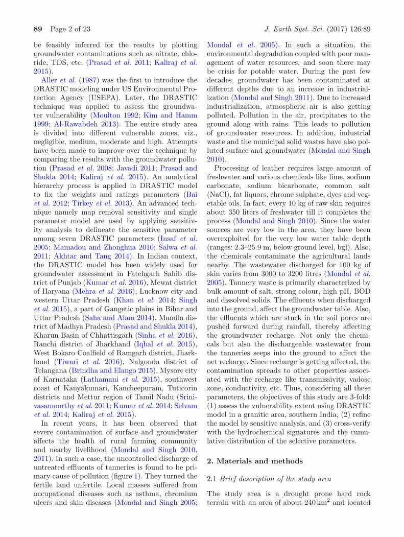
Figure 1. Location of the study area.

in between 10◦13′44′′−10◦26′47′′N latitudes and77◦53′08′′−78◦01′24′′E longitudes (figure 1). Thearea is characterized by undulating topographywith hills (Sirumalai) located in southern parts,sloping towards north and northeast. The eleva-tion (altitude) in plains ranges from 370 m (amsl)in the southern part to 230 m in the northernpart (Mondal et al. 2005). No perennial streamsexist in the area, except for short distance streamsencompassing 2nd and 3rd order drainage (Mon-dal and Singh 2010). Runoff from rainfall withinthe area ends in small streams flowing towards themain Kodaganar River. From a period of 1971–2007, the average annual rainfall is of the orderof 905.3 mm.

2.2 Geological and hydrogeological setup

The study area is covered with Archean granitesand gneisses, intruded by dykes. These rocks arecrossed by sets of joints and fractures, which havealso caused weathering of coarser rocks. The shal-low hard and massive rocks are exposed mostly inthe southern part. Red sandy soil is obtained innorthern and southern parts of the area whereasblack cotton soil occurs in the middle part. Theweathered thickness varies from 3.1 to 26.6 m(Mondal and Singh 2005). Such shallow weatheredzones may not be stable sources of groundwaterfor meeting large demands of groundwater (Singhet al. 2003). There are many lineaments which are


oriented mainly in the NNE–SSW, NEE–SWW,and NW–SE directions, but the major lineamentruns in the NNE–SSW direction for several kilo-meters situated northwest of Dindigul along Koda-ganar River (figure 1). The weathered zone facil-itates the movement and storage of groundwaterthrough a network of joints, faults and lineaments,which form conspicuous structural features. Apartfrom the structural controls on the groundwatermovement, the area is covered with pediment andburied pediment on southern and western sides ofthe area. The other most dominant formation is thecharnockite, which is only found in southern andsoutheastern parts of the Sirumalai hill. This for-mation is less weathered, jointed or fractured com-pared to the previous one and can therefore be con-sidered as impermeable (Mondal and Singh 2005).

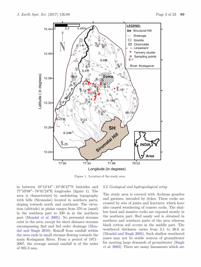
Groundwater occurs mostly in weathered andfractured zones, which are mainly unconfined innature at shallow depth and sometimes semi-con-fined or confined also (Singh et al. 2003). The thick-ness of weathered zone varies from 3.1 to 26.6 m,acting mainly shallow aquifer and its distribu-tion has been shown in Fench diagram (figure 2),which has been prepared with the help of geo-physical survey’s results incorporating the welllogs and cuttings (Mondal and Singh 2011). Theseaquifer confining conditions may change rapidlyand vary over a wide range from place to place. Thethickness of weathered/fractured zone varies overeven a small region. Shallow aquifers (extendedaround 27.68 m, below ground level) are usuallyphreatic condition, which may not be a stablesource for meeting large demands on groundwa-ter, but deeper aquifers (occurred in fracturesbelow the bed rock) are partly-confined/confined,i.e., they are recharged from shallow unconfinedaquifers through dug-cum-bore wells/bore wells aswater accumulates in dug wells, percolates intoconfined aquifers through bore wells which are pro-vided in dug wells. Groundwater is being extractedthrough rope-pulley method from dug well in shal-low aquifer and dug-cum-bore and bore wells indeeper aquifers for their needs.

2.3 Data collection

Seven DRASTIC parameters like groundwatertable, recharge, aquifer discharge, soil types, sur-face elevation, vadose zone thickness and aquiferproperties were collected. The groundwater level,surface elevation, vadose zone thickness and aquiferproperties were collected in the field condition from

the study area. The depths to groundwater tablewere measured at 46 wells. Survey was also car-ried out for the measurement of topography. It wasestimated at 600 locations in grid pattern (200 ×200 m) and incorporated in GIS format to producethe topography map. Vadose zone thickness wascalculated using the groundwater level data at theexisting wells. It varied from 0.52 to 5.35 m. Theinfiltration rate was reported as <1.7 cm/hr (PWD2000). Aquifer properties such as transmissivity(T ) and storativity (S) were estimated throughpumping test at 8 wells (Singh et al. 2003). Tvalues vary from 15 to 200 m2/day, whereas Svalues from 0.0000225 to 0.00095. Aquifer trans-missivity is proportional to hydraulic conductivity(K), which is best defined as an exponential func-tion of aquifer resistivity (Mondal et al. 2016a).Therefore, the calculated T values were directlyused to prepare transmissivity map of the studyarea.

The collateral data like groundwater rechargewas estimated at six PWD wells by entropy method(Mondal et al. 2012). The recharge rate varies from3.37 to 11.10% during the north-east monsoon. Therainfall data was also collected in the year 2001 andit was converted into groundwater recharge whichvaries from 22 to 69 mm/year. It was utilized toprepare recharge map for the DRASTIC model.Although granite is the only geology in the entirestudy area, due to the heterogeneity in hard rockarea, its property of the media changes spatially.Thus, the aquifer media, which serves as aquifer, ischaracterized based on the water level fluctuation(Singh et al. 2003). The water level fluctuation var-ied from 0.00 to 7.20 m which was used for thepreparation of aquifer media map. The soil mapdata had been collected from Public Works Depart-ments (PWD 2000).

The groundwater samples were also collectedfrom 25 representative dug wells and dug-cum-bore wells (figure 1), which were under use at 0.5m below the water table, and were pumped formore than 5 min. Methods of collection and analy-sis of groundwater samples for the cations andanions analysis followed were essentially the sameas given by Brown et al. (1970). Samples were col-lected in 1-litre capacity polythene bottles. Priorto the collection, bottles were thoroughly washedwith diluted HNO3 acid, and then with distilledwater in the laboratory before filling bottles withsamples. Each bottle was rinsed to avoid any pos-sible contamination in bottling and every otherprecautionary measure was taken. WTW portable


Figure 2. Fence diagram showing shallow aquifer.

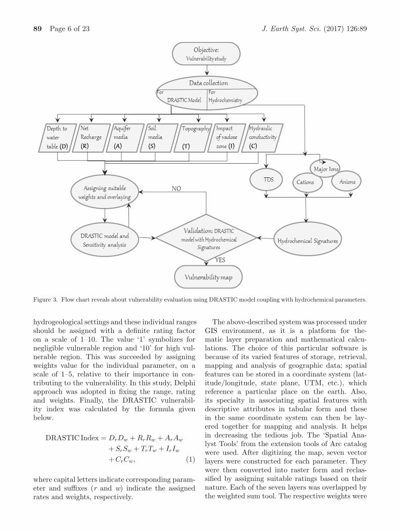
EC and pH meters also measured hydrophysicalparameters, such as pH and EC, on site. Thesedata were used to verify the vulnerability zones ofthe DRASTIC model. The summary of the methodadopted in this study is presented in a flow chart(figure 3).

2.4 DRASTIC model

The DRASTIC modeling was carried out to arriveat groundwater vulnerability zones. The word

DRASTIC is an acronym abbreviated for sevenparameters like depth of water table (D), netrecharge (R), aquifer media (A), soil media (S),topography (T), impact of vadose zone (I) andhydraulic conductivity (C) (table 1). Since theseare the functioning parameters in defining thegroundwater contamination, mapping andoverlapping of these parameters helps in evaluat-ing the degree of susceptibility for groundwaterpollution. The parameters in the DRASTIC modelwere initially divided into ranges for corresponding


Figure 3. Flow chart reveals about vulnerability evaluation using DRASTIC model coupling with hydrochemical parameters.

hydrogeological settings and these individual rangesshould be assigned with a definite rating factoron a scale of 1–10. The value ‘1’ symbolizes fornegligible vulnerable region and ‘10’ for high vul-nerable region. This was succeeded by assigningweights value for the individual parameter, on ascale of 1–5, relative to their importance in con-tributing to the vulnerability. In this study, Delphiapproach was adopted in fixing the range, ratingand weights. Finally, the DRASTIC vulnerabil-ity index was calculated by the formula givenbelow.

DRASTIC Index = DrDw + RrRw + ArAw

+SrSw + TrTw + IrIw

+CrCw, (1)

where capital letters indicate corresponding param-eter and suffixes (r and w) indicate the assignedrates and weights, respectively.

The above-described system was processed underGIS environment, as it is a platform for the-matic layer preparation and mathematical calcu-lations. The choice of this particular software isbecause of its varied features of storage, retrieval,mapping and analysis of geographic data; spatialfeatures can be stored in a coordinate system (lat-itude/longitude, state plane, UTM, etc.), whichreference a particular place on the earth. Also,its specialty in associating spatial features withdescriptive attributes in tabular form and thesein the same coordinate system can then be lay-ered together for mapping and analysis. It helpsin decreasing the tedious job. The ‘Spatial Ana-lyst Tools’ from the extension tools of Arc catalogwere used. After digitizing the map, seven vectorlayers were constructed for each parameter. Theywere then converted into raster form and reclas-sified by assigning suitable ratings based on theirnature. Each of the seven layers was overlapped bythe weighted sum tool. The respective weights were


Table 1. The relative assigned weight (s) of DRASTIC model parameters and its description.

Relative weight(after Aller et al. 1987)

Assigned

relative

weight(s)Factor(s) Description

Depth to water It is the depth from ground surface to the top of

groundwater table, deeper the water level is, the

lesser the chance of contamination

5 5

Net recharge It is an amount of water which recharges the

aquifer, high amount of recharge carries more con-

taminant

4 4

Aquifer media It represents the property which defines the aquifer

matrix like discharge, high discharge constitutes to

high contamination

3 3

Soil media It is the controlling parameter of infiltration, which

represents the soil type, cohesive soils retain the

contaminants than noncohesive soils

2 2

Topography It represents the slope of land surface, gentle undu-

lations sustain the water in a place forcing water

to percolate into the ground

1 1

Impact of vadose zone It is the unsaturated part of earth between ground

surface and top of the phreatic zone, lesser the soil

thickness is higher chance of contaminant interac-

tion with the water table

5 5

Hydraulic conductivity It is the ability of aquifer to transmit water, high

transmissivity injects more contaminants into the

aquifer

3 3

allocated to each of the layers. DRASTIC indexcalculation was performed by default and the finalscore of DRASTIC index was displayed. This indexwas then divided into four zones according to theirscoring value. A high DRASTIC index indicateshigh vulnerability.

2.5 Cumulative probability distribution

Ample of natural earth processes culminate inhydrochemistry of a complex heterogenous aquifer,but this can be reflected in analytical dataset.The probability distributions are considered to beof great importance in dealing with hydrochem-ical data (Mondal et al. 2011). In order to dis-criminate the anomalous population whose chem-istry was affected locally by salinization and/oranthropogenic pollution from a backgroundpopulation, cumulative probability distributions ofhydrochemical parameters were constructed. Inparticular, probability density functions of TDS,Na+ , Cl− and SO2−

4 concentrations were examinedin order to group collected samples on the basisof saline water mixing and anthropogenic pollu-tion as the study area is affected by the untreated

tannery industries. If a chosen groundwater qualityparameter was affected by a single process, theprobability distribution of its concentration formeda unimodal normal or log-normal distribution(Tennant and White 1959). The cumulative proba-bility distribution was then linear on a probabil-ity paper. If the plots of a groundwater qualityparameter did not form a linear distribution, theparameter was considered to be affected by morethan one population (process). For such a case,each population was differentiated by the intersec-tion points of two neighbouring linear populations(Sinclair 1974; Mondal et al. 2016b). Similarly, log–probability plots were adapted here to identify thevulnerability strategies in the study area.

3. Results and discussion

3.1 DRASTIC model

Equation (1) as discussed above was fitted inArcGIS 10.1 software after preparing the DRAS-TIC maps. The weights of each DRASTIC fac-tor was assigned with respect to the other forestimating the relative importance of each


factor (Aller et al. 1987). Although, these factorsare site specific, each factor has been assigneda relative weight ranging from 1 to 5 (table 1).The most significant weightages (5) were given todepth to the water table and impact of vadosezone, whereas comparatively least weightage (1)had been assigned to the topography. Nonethelessthe ratings have a range for each DRASTIC fac-tor with respect to others, and have been assignedbased on the hydrogeological sense prevailing in the

Table 2. GIS-based DRASTIC model parameterrating(s) for the vulnerability study.

Parameter(s) Rating(s)

Depth to water table (m, bgl)

2.30–9.52 10

9.53–12.20 8

12.21–15.07 6

15.08–18.40 4

18.41–25.90 2

Net Recharge (mm/year)

22.42–31.91 2

31.92–38.12 4

38.13–42.50 6

42.51–51.27 8

51.28–64.96 10

Aquifer media (where ΔWL in Zone: in m)

0.00–1.50 2

1.51–3.00 4

3.01–4.50 6

4.5–6.00 8

6.00–7.20 10

Soil media

Red sandy soil 5

Black cotton soil 1

Topography (m, amsl)

230.01–258.43 10

258.44–283.58 7

283.59–308.17 5

308.18–334.96 3

334.97–369.39 1

Impact of vadose zone (m)

0.52–1.41 10

1.42–1.90 8

1.91–2.51 6

2.52–3.59 4

3.60–5.35 2

Transmissivity (m2/day)

15.00–51.27 2

51.28–81.02 3

81.03–115.83 5

115.84–156.73 7

156.74–199.96 9

study area. The ratings, which varied from 1 to10, have been assigned for the DRASTIC factor asper the specific hydrogeological knowledge. Speci-fied ratings (table 2) were given for different ranges.It shows the weights portioned for seven parame-ters of DRASTIC model and ratings for individualrange.

3.1.1 Depth to water table

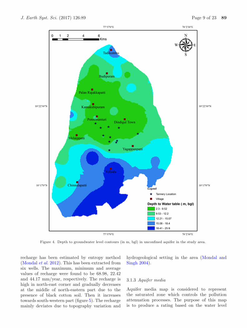
Depth to groundwater table is a significant factorin DRASTIC modeling as it affects the verticaltravel time of contaminant from surface poundage(Stigter et al. 2006). It is the surface where thewater pressure head is equal to the atmosphericpressure (pressure where gauge pressure is zero).Water table was collected at 46 wells; 25.90, 2.30and 11.97 m are the maximum, minimum andaverage values of the dataset, while 5.28 m isthe standard deviation. The groundwater levelcontours were interpolated with the help of krig-ing method. Highest rating (10) was assigned tolow water table locations (range: 2.30–9.52 m, intable 2) as it is inversely related to the ground-water contamination. If the depth to water level islow from ground surface, then the time of travel forpollutant to reach the water table is less. Hence, itwas assigned with highest rating (10). The watertable contour map shown in figure 4 gives real-time demarcation in the experimental site. Sincethere are high hills located in the south-east region,there was comparatively deeper water table andrunoff from the hills spreads over the hills footarea. The depth gradually decreases towards cen-tral part where the tannery clusters are located(figure 1).

3.1.2 Recharge

Recharge basically represents the amount of waterthat infiltrates into the ground. High recharge indi-cates high infiltration. As the infiltration containspollutants, the rate of contamination increases withhigh recharge. Hence, a proportional rating hasbeen assigned for the recharge values as a highrecharge implies high contamination infiltrated intothe ground. Since the DRASTIC model was devel-oped for uniform rainfall distribution and naturalland surfaces, it is not applicable for the cityDindigul. The area has very low degree of precipita-tion and moderate undulations (Mondal and Singh2012a). Thus, the monsoon data from January 1973to December 2007 has been considered and the


Figure 4. Depth to groundwater level contours (in m, bgl) in unconfined aquifer in the study area.

recharge has been estimated by entropy method(Mondal et al. 2012). This has been extracted fromsix wells. The maximum, minimum and averagevalues of recharge were found to be 68.98, 22.42and 44.17 mm/year, respectively. The recharge ishigh in north-east corner and gradually decreasesat the middle of north-eastern part due to thepresence of black cotton soil. Then it increasestowards south-western part (figure 5). The rechargemainly deviates due to topography variation and

hydrogeological setting in the area (Mondal andSingh 2004).

3.1.3 Aquifer media

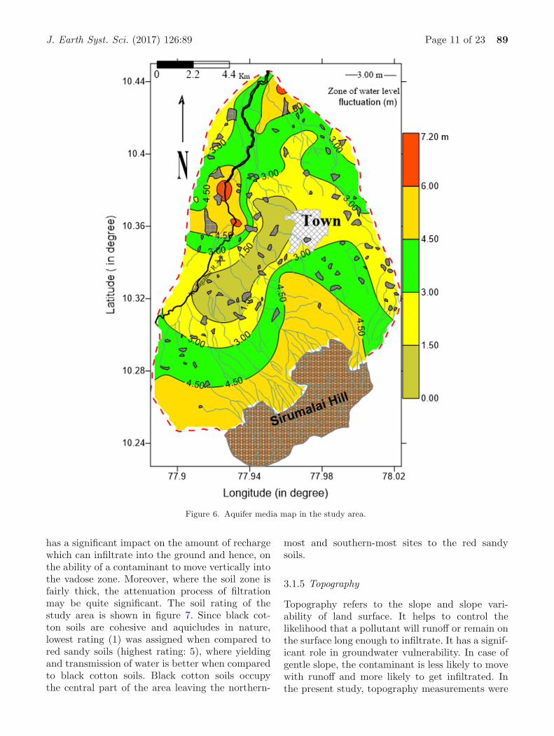
Aquifer media map is considered to representthe saturated zone which controls the pollutionattenuation processes. The purpose of this mapis to produce a rating based on the water level


Figure 5. Recharge rate (mm/year) distribution in the study area.

fluctuation of aquifer media. The aquifer mediamap (figure 6) of the study area has been preparedby estimating the water level fluctuation in the fieldcondition (Singh et al. 2003). The change of waterlevel varies from 0.00 to 7.20 m. High groundwaterlevel fluctuation allows more contaminants to enterthe aquifer. Therefore, a high fluctuation (range:6.00–7.20 m) will yield a high vulnerability rating(figure 6). The aquifer fluctuation is high in the

northern and north-western parts and decreasesspatially on either direction.

3.1.4 Soil media

Soil media refers to the upper most portion ofvadose zone characterized by significant biologicalactivity (Aller et al. 1987). In this study, only theupper weathered zone has been considered. Soil


Figure 6. Aquifer media map in the study area.

has a significant impact on the amount of rechargewhich can infiltrate into the ground and hence, onthe ability of a contaminant to move vertically intothe vadose zone. Moreover, where the soil zone isfairly thick, the attenuation process of filtrationmay be quite significant. The soil rating of thestudy area is shown in figure 7. Since black cot-ton soils are cohesive and aquicludes in nature,lowest rating (1) was assigned when compared tored sandy soils (highest rating: 5), where yieldingand transmission of water is better when comparedto black cotton soils. Black cotton soils occupythe central part of the area leaving the northern-

most and southern-most sites to the red sandysoils.

3.1.5 Topography

Topography refers to the slope and slope vari-ability of land surface. It helps to control thelikelihood that a pollutant will runoff or remain onthe surface long enough to infiltrate. It has a signif-icant role in groundwater vulnerability. In case ofgentle slope, the contaminant is less likely to movewith runoff and more likely to get infiltrated. Inthe present study, topography measurements were


Figure 7. Soil distribution of the study area.

done in the field condition and it varies from 230m (amsl) in the northern part to 370 m (amsl)in the southern part. The ratings were used forthe analysis as presented in table 2 and shown infigure 8.

3.1.6 Impact of vadose zone

The vadose zone, also termed the unsaturated zone,is the part of Earth between land surface and

the top of phreatic zone, the position at whichthe groundwater (the water in the soil’s pores) isat atmospheric pressure. Hence, the vadose zoneextends from the top of the ground surface tothe water table. But this table is being fluctuatedseasonally and year-wise in any watershed. Theinfiltrated water reaches the groundwater throughthis zone. However, when evaluating the model,the word has been expanded to include boththe vadose zone and any saturated zones which


Figure 8. Topography pattern in the study area.

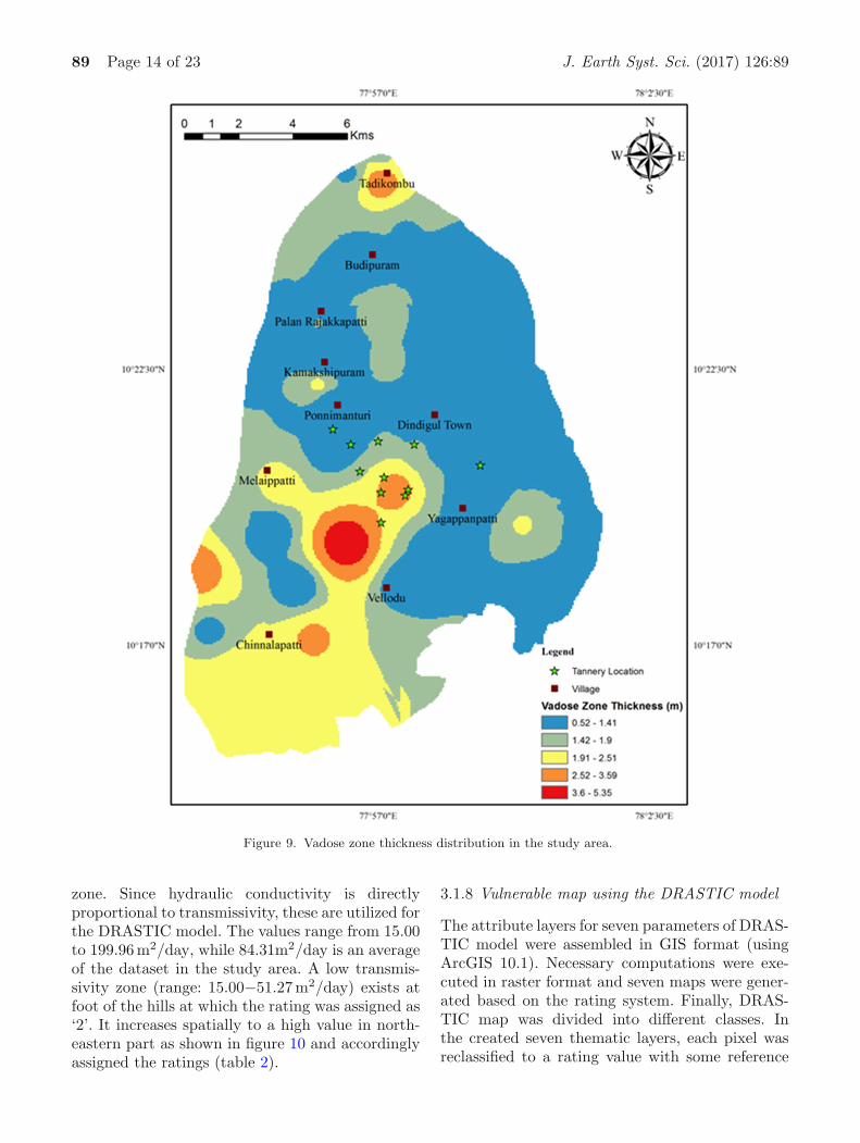
overlie the shallow aquifer. The vadose zones wereconsidered as the depth of regional average waterlevel (bgl) measured in the last 3–4 decades at thePDW wells. It ranges between 0.52 and 5.35 m, bglwith an average of 1.59 m in the study area.

The aquifer media controls the path length androuting as the water flows into the aquifer. Thickerthe zone, longer is the path length and thus affect-ing the travel time of pollutant in groundwater.Hence, an inversely proportional relation has beengiven to the vadose zone map, i.e., low rating (=2)

to the thicker vadose area (range: 3.60–5.35 m).Low to medium thickness ranges all over the areawere considered except at few places where thethickness range is more as shown in figure 9.

3.1.7 Conductivity

Conductivity represents the property of aquiferto transmit water. High groundwater flow raterepresents high contaminant advection; hence ahigh rating was assigned to high conductivity


Figure 9. Vadose zone thickness distribution in the study area.

zone. Since hydraulic conductivity is directlyproportional to transmissivity, these are utilized forthe DRASTIC model. The values range from 15.00to 199.96 m2/day, while 84.31m2/day is an averageof the dataset in the study area. A low transmis-sivity zone (range: 15.00−51.27 m2/day) exists atfoot of the hills at which the rating was assigned as‘2’. It increases spatially to a high value in north-eastern part as shown in figure 10 and accordinglyassigned the ratings (table 2).

3.1.8 Vulnerable map using the DRASTIC model

The attribute layers for seven parameters of DRAS-TIC model were assembled in GIS format (usingArcGIS 10.1). Necessary computations were exe-cuted in raster format and seven maps were gener-ated based on the rating system. Finally, DRAS-TIC map was divided into different classes. Inthe created seven thematic layers, each pixel wasreclassified to a rating value with some reference


Figure 10. Transmissivity distribution in the study area.

or by Delphi method. The reclassification tool inspatial analyst tool box was used to reclassify eachpixel. These reclassified maps were overlaid bythe weighted sum tool in the spatial analyst toolbox. The process of multiplying reclassified rat-ing of each pixel with the weight given to definiteparameter was carried out. Finally, the vulnera-bility index or DRASTIC index was calculated.Total DRASTIC index varied from 39 to 132 forthe vulnerability. The resulted index was dividedinto four equal groups (Aller et al. 1987). Small

numbers indicate low vulnerability potential andlarge numbers were related to those areas that havehigh vulnerability in respect to pollution. Theyrepresent on a DRASTIC map (figure 11) andthe corresponding values for each point were alsoextracted.

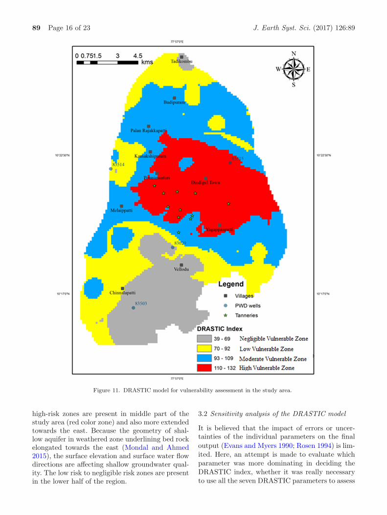
DRASTIC vulnerable map (figure 11) shows thatabout 103.2 km2 (43%) of the area lies between lowto negligible risk of pollution zone but the remain-ing about 136.8 km2 (57%) is occupied by moderaterisk to high risk of pollution zone (table 3). The


Figure 11. DRASTIC model for vulnerability assessment in the study area.

high-risk zones are present in middle part of thestudy area (red color zone) and also more extendedtowards the east. Because the geometry of shal-low aquifer in weathered zone underlining bed rockelongated towards the east (Mondal and Ahmed2015), the surface elevation and surface water flowdirections are affecting shallow groundwater qual-ity. The low risk to negligible risk zones are presentin the lower half of the region.

3.2 Sensitivity analysis of the DRASTIC model

It is believed that the impact of errors or uncer-tainties of the individual parameters on the finaloutput (Evans and Myers 1990; Rosen 1994) is lim-ited. Here, an attempt is made to evaluate whichparameter was more dominating in deciding theDRASTIC index, whether it was really necessaryto use all the seven DRASTIC parameters to assess


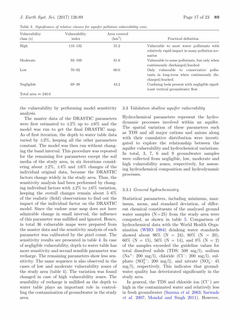
Table 3. Significance of relative classes for aquifer pollution vulnerability zone.

Vulnerability

class (s)

Vulnerability

index

Area covered

(km2) Practical definition

High 110–132 55.2 Vulnerable to most water pollutants with

relatively rapid impact in many pollution sce-

narios

Moderate 93–109 81.6 Vulnerable to some pollutants, but only when

continuously discharged/leached

Low 70–92 60.0 Only vulnerable to conservative pollu-

tants in long-term when continuously dis-

charged/leached

Negligible 69–39 43.2 Confining beds present with negligible signif-

icant vertical groundwater flow

Total area = 240.0

the vulnerability by performing model sensitivityanalysis.

The master data of the DRASTIC parameterswere first estimated to ±2% up to ±6% and themodel was run to get the final DRASTIC map.As of first iteration, the depth to water table datavaried by ±2%, keeping all the other parametersconstant. The model was then run without chang-ing the band interval. This procedure was repeatedfor the remaining five parameters except the soilmedia of the study area, in six iterations consid-ering about ±2%, ±4% and ±6% changes of theindividual original data, because the DRASTICfactors change widely in the study area. Thus, thesensitivity analysis had been performed by chang-ing individual factors with ±2% to ±6% variation,keeping the overall changes remain about 5–6%of the realistic (field) observations to find out theimpact of the individual factor on the DRASTICmodel. Since the vadose zone map does not haveadmirable change in small interval, the influenceof this parameter was nullified and ignored. Hence,in total 36 vulnerable maps were prepared fromthe master data and the sensitivity analysis of eachparameter was calibrated by the pixel count. Thesensitivity results are presented in table 4. In caseof negligible vulnerability, depth to water table hasmore sensitivity and second sensible parameter wasrecharge. The remaining parameters show less sen-sitivity. The same sequence is also observed in thecases of low and moderate vulnerability zones ofthe study area (table 4). The variation was foundchanged in case of high vulnerability zones. Thesensibility of recharge is nullified as the depth towater table plays an important role in control-ling the contamination of groundwater in the studyarea.

3.3 Validation shallow aquifer vulnerability

Hydrochemical parameters represent the hydro-dynamic processes involved within an aquifer.The spatial variation of these parameters suchas TDS and all major cations and anions alongwith their cumulative distribution were investi-gated to explore the relationship between theaquifer vulnerability and hydrochemical variations.In total, 3, 7, 6 and 9 groundwater sampleswere collected from negligible, low, moderate andhigh vulnerability zones, respectively, for assess-ing hydrochemical composition and hydrodynamicprocesses.

3.3.1 General hydrochemistry

Statistical parameters, including minimum, max-imum, mean, and standard deviation, of differ-ent chemical constituents of the analyzed groundwater samples (N=25) from the study area werecomputed, as shown in table 5. Comparison ofhydrochemical data with the World Health Orga-nization (WHO 1984) drinking water standardsshowed about 96% (N = 24), 80% (N = 20),60% (N = 15), 56% (N = 14), and 8% (N = 2)of the samples exceeded the guideline values fortotal dissolved solids (TDS: 500 mg/l), sodium(Na+: 200 mg/l), chloride (Cl−: 200 mg/l), sul-phate (SO2−

4 : 200 mg/l), and nitrate (NO−3 : 45

mg/l), respectively. This indicates that ground-water quality has deteriorated significantly in thestudy area.

In general, the TDS and chloride ion (Cl−) arehigh in the contaminated water and relatively lessin fresh groundwater (Saxena et al. 2003; Sarwadeet al. 2007; Mondal and Singh 2011). However,


Table 4. Showing (A) high, (B) moderate, (C) low, and (D) negligible vulnerability pixels by changing the DRASTICparameter(s) in the study area.

Changing

factor(s)

Depth to

water level

Net

recharge

Aquifer

media

Impact of

vadose zone

Hydraulic

conductivityTopography

(A) For high vulnerability zone

−6% 4881 2751 2419 2864 2771 2901

−4% 3473 2751 2419 2861 2771 2901

−2% 2718 2833 2504 2834 2764 2911

Field data 2381 2381 2381 2381 2381 2381

2% 2221 2499 2869 2764 2628 2710

4% 2133 2805 2967 2715 2769 2724

6% 2956 2885 2608 2670 2723 2923

(B) For moderate vulnerability zone

−6% 3093 5154 5566 5322 5363 5184

−4% 3694 5154 5566 5278 5363 5184

−2% 4374 5151 5521 5281 5381 5174

Field data 3678 3678 3678 3678 3678 3678

2% 2991 3380 5296 5310 5420 5415

4% 2837 5394 5226 5336 5258 5413

6% 4095 5161 5450 5336 5392 5166

(C) For low vulnerability zone

−6% 1240 1845 1773 1733 1826 1709

−4% 1193 1845 1773 1733 1826 1697

−2% 1821 1818 1755 1724 1828 1704

Field data 2666 2666 2666 2666 2666 2666

2% 3361 2857 1665 1726 1686 1778

4% 3533 1675 1645 1813 1674 1737

6% 1992 1829 1740 1716 1827 1751

(D) For negligible vulnerability zone

−6% 1383 794 760 732 672 706

−4% 436 794 760 732 672 765

−2% 1688 760 766 750 676 782

Field data 1876 1876 1876 1876 1876 1876

2% 2028 1865 771 827 790 749

4% 2098 727 763 761 788 813

6% 1558 677 775 770 681 842

bicarbonate (HCO−3 ) is dominant in fresh ground-

water than that of saline water. The molar ratio ofCl−/HCO−

3 is referred to as the Revelle coefficient(Revelle 1941) and could be appraised as intensityof salinity into the shallow aquifer. Hence, thesehydrochemical parameters have been used to ver-ify the site-specific vulnerability towards shallowaquifer contamination.

The result shows that the samples that fallwithin the negligible vulnerable zones have com-paratively low concentration of TDS (650–1389mg/l), Na+ (47–161 mg/l), Cl− (106–298 mg/l),HCO−

3 (340–500 mg/l) and the molar ratios Cl−/HCO−

3 ranges from 0.54 – 1.03. These valuesare relatively low in the southern and northernparts than other parts of the study area (table 5,

figure 12). In this area, the aquifers are foundto have low vulnerability due to the subsequentreplenishment of fresh water by infiltration fromthe Sirumalai Hill.

But the samples from the high vulnerable zones(in and around the tannery clusters) have high con-centration of TDS (2,304–39,100 mg/l), Na+ (239–6,046 mg/l), Cl− (532–13,652 mg/l), and the molarratios Cl−/HCO−

3 ranges from 1.43 to 106.81. Thisarea is highly susceptible to the advection of con-taminants in the form of pollutants (Mondal andSingh 2012b). The moderate vulnerability condi-tions were observed around the highly vulnerablezones having a moderate hydrochemical concen-trations of TDS (1204–3976 mg/l), Na+ (182–654mg/l), Cl− (213–1596 mg/l), and the molar ratios


Table 5. Minimum, maximum, mean and standard deviation of the selective groundwater samples forthe study area in comparison with the worldwide average surface water and groundwater.

Parameters pH EC TDS Ca2+ Mg2+ Na+ K+ HCO−3 Cl− SO2−

4 NO−3

Negligible vulnerability zone (sample nos. 3: 23, 20 & 24)

Minimum 7.05 1166 650 71 74 47 2 340 106 86 4

Maximum 7.71 2170 1389 182 88 161 32 500 298 240 55

Mean 7.42 1763 1103 120 82 112 12 440 224 145 21

Std. Dev. 0.33 528 396 57 7.3 59 17 87 103 83 29

Low vulnerability zone (sample nos. 7: 2, 6, 8, 17, 10, 22 & 25)

Minimum 7.56 780 499 56 22 43 2 214 57 25 2

Maximum 8.25 2640 1796 173 110 295 16 420 418 290 10

Mean 7.91 1478 935 111 48 123 5 312 227 96 4.5

Std. Dev. 0.23 684 476 42 31 90 5.1 60 161 91 3.4

Moderate vulnerability zone (sample nos. 6: 1, 3, 7, 11, 18 & 21)

Minimum 7.31 1854 1204 83 31 182 2 280 213 110 5

Maximum 8.24 5912 3976 433 176 654 12 520 1596 263 15

Mean 7.79 3441 2341 223 93 354 6.1 376 807 192 8.1

Std. Dev. 0.32 1750 1241 134 61 172 3.3 84 605 64 3.6

High vulnerability zone (sample nos. 9: 4, 5, 9, 10, 12, 13, 14, 15 &16)

Minimum 6.44 3300 2304 161 73 239 6 200 532 254 6

Maximum 8.23 54000 39100 2490 1854 6046 62 640 13652 7154 87

Mean 7.54 10626 7732 587 319 1160 16 375 2641 1149 18

Std. Dev. 0.51 16414 11894 733 580 1859 17 164 4189 2257 26

Standards

For PLDW 6.5-8.5 — 500 75 30 200 100 200 200 200 45

For SW — — — 13.4 3.4 5.2 1.3 — 5.8 8.3 —

For GW — — — 50 7 30 3 — 20 30 —

All ions in mg/l except EC in µS/cm, pH: -log10H+; collected 25 groundwater samples on February

2009. PLDW: Permissible limit for drinking water (WHO 1984); SW: average surface water afterMeybeck (1979) and GW: average groundwater after Turekian (1977).

Figure 12. Comparative values of SO2−4 , Na+, Cl− and TDS (in mg/l) in the groundwater samples for the negligible, low,

moderate and high vulnerability zones (except sample no. 13).

Cl−/HCO−3 ranges from 0.77–8.28. The SO2−

4 con-centration ranges from 110 to 263 mg/l and theNO−

3 concentration ranges between 5 and 15 mg/l,

indicating comparatively fair groundwater quality.The movement of groundwater is slower in theblack cotton soil area due to poor porosity and


permeability. It reduces the groundwater flow andthus groundwater contamination (Mondal and Singh2012b). The comparatively lower values of TDS(499–1796 mg/l) and Cl− (57–418 mg/l) werenoticed in the northern and southern parts of thestudy area which is underlain by the low vulnerablezones.

3.3.2 Cumulative probability distributionfor, hydrochemical processes

Most of the hydrochemical parameters obtained inthis study exhibited log-normal density distribu-tions. It is noticed that Na+, Cl− and SO2−

4 weremajor constituents of the tannery effluent, becauseleather industries use various chemicals like sodiumcarbonate, sodium bicarbonate, sodium chloride(NaCl), chrome sulphate, etc., in the study area(Mondal and Singh 2010). However, the occur-rence of an anomalous population as a ‘tail’on the distribution suggested that groundwaterchemistry was controlled by several intermixingprocesses. The frequency plots of Na+, Cl− and

SO2−4 concentrations including TDS showed a

log-normal distribution, but had a tail at highconcentration ranges. In the study area, the regi-onal background values of TDS, Na+, Cl− andSO2−

4 were about 1200, 165, 190 and 69 mg/l,respectively. This indicated that several numbersin the samples with high Na+, Cl− and SO2−

4

concentrations can be attributed to an anomalouspopulation whose chemistry was locally affected bythe effluent water mixing and others in the highvulnerability zone.

Cumulative probability distributions of TDS,Na+, Cl− and SO2−

4 are shown in figure 13(a–d). There are 2–4 individual intersection pointson the cumulative probability plots, which canbe considered as regional threshold values andhighly impacted threshold values for differentiatingthe samples with the effects of geogenic, anthro-pogenic and saline water mixing from the untreatedeffluents. The first approximate regional thresh-old values obtained were 1200 mg/l for TDS,165 mg/l for Na+, 190 mg/l for Cl−, and 69mg/l for SO2−

4 (figure 13). Broadly, the samples

Figure 13. Cumulative probability distribution of TDS, Na+, Cl− and SO2−4 (in mg/l) for the groundwater samples in the

negligible, low, moderate and high vulnerability zones (except sample no. 13).


have less than the first threshold values of thesehydrochemical parameters fallen in the negligibleand less vulnerability zones in the study area.Simultaneously, the second estimated highlyimpacted threshold values were 1300, 425, 400 and225 mg/l for TDS, Na+, Cl−, and SO2−

4 , respec-tively. The samples located in the moderate andhighly vulnerability zones, fallen on the third seg-ment for the Na+, Cl−, and SO2−

4 concentrationsbut in the 2−4th segments of TDS on the cumula-tive probability curves. These were highly affectedby the tannery effluents. The five samples havefallen on the last segments for Na+, Cl−, andSO2−

4 concentration and the 4th segment for theTDS within the high vulnerable zones which aremainly located in and around the tannery clusters.These have been recorded with high concentrationof TDS (3976–6895 mg/l), Na+ (434–1,090 mg/l),Cl− (1347–2517 mg/l), and SO2−

4 (310–721 mg/l).It shows that the cumulative probability distri-bution of the hydrochemical parameters directlyindicate the vulnerability zones for the shallowaquifer in the hard rock area.

4. Conclusions

An attempt has been made to assess the shal-low aquifer vulnerability using DRASTIC index ina granitic terrain of southern India. The resultsshow that about 43% of the area is healthy withlittle vulnerability. The remaining 57% of thearea is highly polluted. This is mainly becauseof the tannery industries which release untreatedwaste water into the ground. The pollution hasalso reached to the surrounding agricultural farmshence polluting the land as well as the productioncoming from the land. The sensitivity analysis ofthe DRASTIC model has resulted in delineatinghigh vulnerability zones where the depth to watertable is a driving force for controlling the ground-water contamination.

The hydrochemical parameters such as TDS,Cl−, HCO−

3 , SO2−4 and Cl−/HCO−

3 molar ratioshave been analyzed to verify the efficiency of thevulnerability. The samples falling in the high vul-nerable zone have been recorded with high concen-tration of TDS (2304–39,100 mg/l), Na+ (239–6046mg/l), Cl− (532–13,652 mg/l), and the molar ratiosCl−/HCO−

3 ranges from 1.43–106.81. The low con-centrations of TDS (650–1389 mg/l), Na+ (47–161mg/l), Cl− (106–298 mg/l), HCO−

3 (340–500 mg/l)

and the molar ratios Cl−/HCO−3 (0.54–1.03) are

observed within the negligible vulnerable zone(s).The cumulative probability distributions of TDS,

Na+, and Cl− constituents show 2–4 individualintersection points on the cumulative probabilityplots. The concentrations of TDS, Na+, and Cl−

in groundwater in the negligible vulnerable zoneare found to be in the first regional thresholdvalues obtained as 1200 mg/l for TDS, 165 mg/lfor Na+, and 190 mg/l for Cl−, whereas the sec-ond threshold values, 1300, 425, and 400 mg/l forTDS, Na+, and Cl−, respectively, in the high vul-nerable zone. The hydrochemical results are foundto be well correlated with the DRASTIC model inthe study area. Hence, the vulnerability assessmentthrough the DRASTIC model in any hydrogeo-logical system along with hydrochemical signa-tures is important for sustainable groundwatermanagement.

Acknowledgements

The authors are thankful to Dr. V M Tiwari,Director of CSIR-NGRI, Hyderabad, India who hasencouraged and given the permission to publishthis article. The work has been carried out underthe NGRI-CSIR In-House Project (MLP-6407).They also thank the two anonymous reviewers fortheir constructive comments to improve the article.

References

Akhtar M M and Tang Z 2014 Evaluation of local ground-water vulnerability based on DRASTIC index method inLahore, Pakistan; Geofisica Int. 54(1) 67–81.

Albinet M and Margat J 1970 Cartographie de la vulnerabilite a la pollution des nappes d’eau souterraines. (Map-ping aquifer vulnerability to pollution) in French; Bull.BRGM 2(3–4) 13–22.

Aller L, Bennet T, Leher J H, Petty R J and Hackett G 1987DRASTIC: A standardized system for evaluating ground-water pollution potential using hydrogeological setting;EPA 600/2–87–035 622.

Al-Rawabdeh AM 2013 GIS-based DRASTIC model forassessing aquifer vulnerability in Amman-Zerqa ground-water basin, Jordan; J. Sci. Res. 5 490–504.

Bai L, Wang Y and Meng F 2012 Application of DRASTICand extension theory in the groundwater vulnerabilityevaluation; Water Environ. J. 2(3) 381–391.

Brindha K and Elango L 2015 Cross comparison of five popu-lar groundwater pollution vulnerability index approaches;J. Hydrol. 524 595–613.

Browen E, Skougstad M W and Fishman M J 1970 Methodfor collection and analysis of water samples for dissolvedmineral and gasses; US Govt. Printing Office, Washington.


Evans BM and Myers W L 1990 A GIS-based approach toevaluating regional groundwater pollution potential withDRASTIC; J. Soil Water Conserv. 45(2) 242–245.

Insaf S B, Mohamed A A M, Tetsuya H and Kikuo K 2005 AGIS-based DRASTIC model for assessing aquifer vulner-ability in Kakamigahara Heights, Gifu Prefecture, centralJapan; Sci. Total Environ. 345(1–3) 127–140.

Iqbal J, Pathak G and Gorai A K 2015 Development ofhierarchical fuzzy model for groundwater vulnerability topollution assessment; Arab J. Geosci. 8 2713–2728.

Javadi K N 2011 Modification of DRASTIC model tomap groundwater vulnerability to pollution using nitratemeasurements in agricultural areas; J. Agri. Sci. Tech. 13239–249.

Kaliraj S, Chandrasekar N, Simon Peter T, Selvakumar Sand Magesh N S 2015 Mapping of coastal aquifer vulner-able zone in the south west coast of Kanyakumari, southIndia, using GIS-based DRASTIC model; Environ. Monit.Assess. 187 4073.

Khan A, Khan H H, Umar R and Khan M H 2014 An inte-grated approach for aquifer vulnerability mapping usingGIS and rough sets: Study from an alluvial aquifer innorth India; Hydrogeol. J. 22 1561–1572.

Kim Y J and Hamm S 1999 Assessment of the potential forgroundwater contamination using DRASTIC/EGIS tech-nique, Cheonghu area, South Korea; Hydrol. J. 7 227–235.

Kumar P, Debnath S K, Thakur P K and Bansod B K S 2016Assessment of the effectiveness of DRASTIC in predict-ing the vulnerability of groundwater to contamination: Acase study from Fatehgarh Sahib district in Punjab, India;Environ. Earth Sci. 75 879.

Kumar S, Thirumalaivasan D and Radhakrishnan N 2014GIS based assessment of groundwater vulnerability usingdrastic model; Arab J. Sci. Eng. 39 207–216.

Lathamani R, Janardhana, M R, Mahalingam B and SureshaS 2015 Evaluation of aquifer vulnerability using DrasticModel and GIS: A case study of Mysore City, Karnataka,India; Aquatic Procedia 4 1031–1038.

Mamadou S and Zhonghua T 2010 Assessment of ground-water pollution potential of the Datong Basin, northernChina; J. Sust. Dev. 3(2) 140–152.

Mehra M, Oinam B and Singh C K 2016 Integrated assess-ment of groundwater for agricultural use in Mewat districtof Haryana, India using geographical information system(GIS); J. Indian Soc. Remote Sens. 44(5) 747–758.

Meybeck M 1979 Concentrations des eaux fluviales en ele-ments majeurs et apports en solution aux oceans; Rev.Geol. Dyn. Geogr. Phys. 21 215–246.

Mondal N C and Ahmed S 2015 Dar-Zarrouk parameters fordeducing shallow fresh groundwater zones in a tannerybelt, Tamil Nadu, India; J. Geophys. 36(4) 175–185.

Mondal N C and Singh V P 2010 Need of groundwater man-agement in tannery belt: A scenario about Dindigul town,Tamil Nadu; J. Geol. Soc. India 76(3) 303–309.

Mondal N C and Singh V P 2011 Hydrochemical analysisof salinization for a tannery belt in southern India; J.Hydrol. 405(2-3) 235–247.

Mondal N C and Singh V P 2012a Evaluation of ground-water monitoring network of Kodaganar River basin fromsouthern India using entropy; Environ. Earth Sci. 66(4)1183–1193.

Mondal N C and Singh V P 2012b Chloride migration ingroundwater for a tannery belt in southern India; Environ.Monit. Assess. 184(5) 2857–2879.

Mondal N C and Singh V S 2004 A new approach to delineatethe groundwater recharge zone in hard rock terrain; Curr.Sci. 87(5) 658–662.

Mondal N C and Singh V S 2005 Modeling for pollutantmigration in the tannery belt, Dindigul, Tamilnadu, India;Curr. Sci. 89(9) 1600–1606.

Mondal N C, Saxena V K and Singh V S 2005 Assessmentof groundwater pollution due to tanneries in and aroundDindigul, Tamilnadu, India; Environ. Geol. 48(2) 149–157.

Mondal N C, Singh V P, Singh S and Singh V S 2011 Hydro-chemical characteristic of coastal aquifer from Tuticorin,Tamil Nadu, India; Environ. Monit. Assess. 175(1–4)531–550.

Mondal N C, Singh V P and Ahmed S 2012 Entropy-basedapproach for assessing natural recharge in unconfinedaquifers from southern India; Water Res. Manag. 26(9)2715–2732.

Mondal N C, Bhuvaneswari Devi A, Anand Raj P, Ahmed Sand Jayakumar K V 2016a Estimation of aquifer parame-ters from surfacial resistivity measurement in granitic areain Tamil Nadu; Curr. Sci. 111(3) 524–534.

Mondal N C, Tiwari K K, Sharma K C and Ahmed S 2016bA diagnosis of groundwater quality from a semiarid regionin Rajasthan, India; Arab. J. Geosci. 9(12) 1–22.

Moulton D L 1992 DRASTIC analysis of the potential forgroundwater pollution in Pinal County, Arizona; ArizonaGeological Survey, 11 Sheets, 67.

Prasad K and Shukla J P 2014 Assessment of groundwatervulnerability using GIS-based DRASTIC technology forthe basaltic aquifer of Burhner watershed, Mohgaon block,Mandla (India); Curr. Sci. 107(10) 1649–1656.

Prasad R K, Mondal N C, Banerjee P, Nandakumar M V andSingh V S 2008 Deciphering potential groundwater zone inhard rock through the application of GIS; Environ. Geol.55(3) 467–475.

Prasad R K, Singh V S, Krishnamacharyulu S K and Baner-jee P 2011 Application of DRASTIC model and GIS: Forassessing vulnerability in hard rock granitic aquifer; Env-iron. Monitor. Assess. 176 143–155.

Public Works Department (PWD) 2000 Groundwater per-spective – a profile of Dindigul District, Tamilnadu.Chennai, India, 102p.

Revelle R 1941 Criteria for recognition of seawater in ground-waters; Trans. Am. Geophys. Union 22 593–597.

Rosen L 1994 A study of the DRASTIC methodology withemphasis on Swedish conditions; Ground Water 32(2)278–285.

Saha D and Alam F 2014 Groundwater vulnerability assess-ment using DRASTIC and Pesticide DRASTIC modelsin intense agriculture area of the Gangetic plains, India;Environ. Monit. Assess. 186 8741–8763.

Salwa S, Salem B and Hamed B D 2011 Sensitivity analysis ingroundwater vulnerability assessment based on GIS in themahdia-Ksour Essaf aquifer, Tunisia: A validation study;J. Hydrol. Sci. 56(2) 288–304.

Sarwade D V, Nandakumar M V, Kesari M P, Mondal N C,Singh V S and Bhoop Singh 2007 Evaluation of seawater


ingress into an Indian Attoll; Environ. Geol. 52(2) 1475–1483.

Saxena V K, Singh V S, Mondal N C and Jain S C 2003Use of hydrochemical parameters for the identification offresh groundwater resources, Potharlanka Island, India;Environ. Geol. 44(5) 516–521.

Selvam S, Magesh N S, Sivasubramanian P, ManimaranG, Soundranayagam J P and Seshunarayana T 2014Deciphering of groundwater potential zones in Tuticorin,Tamil Nadu, using remote sensing and GIS techniques;J. Geol. Soc. India 84 597–608.

Sinclair A J 1974 Selection of thresholds in geochemicaldata using probability graphs; J. Geochem. Explor. 3 129–149.

Singh A, Srivastav S K, Kumar S and Chakrapani G J 2015 Amodified-DRASTIC model (DRASTICA) for assessmentof groundwater vulnerability to pollution in an urbanizedenvironment in Lucknow, India; Environ. Earth Sci. 745475–5490.

Singh V S, Mondal N C, Ron Barker, Thangarajan M, RaoT V and Subramaniyam K 2003 Assessment of ground-water regime in Kodaganar river basin (Dindigul dis-trict), Tamilnadu; Tech. Rept. No.-NGRI-2003-GW-269,p. 104.

Sinha M K, Verma M K, Ahmad I, Baier K, Jha R andAzzam R 2016 Assessment of groundwater vulnerability

using modified DRASTIC model in Kharun Basin, Chhat-tisgarh, India; Arab J. Geosci. 9 98.

Srinivasamoorthy K, Vijayaraghavan K, Vasanthavigar M,Sarma V S, Rajivgandhi R, Chidambaram S, Anandhan Pand Manivannan R 2011 Assessment of groundwater vul-nerability in Mettur region,Tamilnadu, India using drasticand GIS techniques; Arab J. Geosci. 4 1215–1228.

Stigter T Y, Ribeiro L and Dill A 2006 Evaluation of anintrinsic and a specific vulnerability assessment methodin comparison with groundwater stalinization and nitratecontamination levels in two agricultural regions in theSouth of Portugal; Hydrol. J. 14(1–2) 79–99.

Tennant C B and White M L 1959 Study of the distributionof some geochemical data; Econ. Geol. 54 1281–1290.

Tirkey K, Gorai A K and Iqbal K 2013 AHP-GIS basedDRASTIC model for groundwater vulnerability to pol-lution assessment: A case study of Hazaribag district,Jharkhand, India; Int. J. Environ. Protec. 2(3) 20–31.

Tiwari A K, Singh P K and Maio M D 2016 Evaluation ofaquifer vulnerability in a coal mining of India by usingGIS-based DRASTIC model; Arab J. Geosci. 9 438.

Turekian K K 1977 Geochemical distribution of elements; 4thedn, Encyclopedia of Science and Technology; McGraw-Hill, New York, 630p.

World Health Organization (WHO) 1984 Guideline of drink-ing quality; World Health Organization, Washington.

Corresponding editor: Rajib Maity

determining shallow aquifer vulnerability by the drastic

Documents