Received 8 December 2015; revised 20 February 2016; accepted 22 February 2016. Date of publication 1 March 2016; date of current version 22 April 2016.The review of this paper was arranged by Editor A. G. U. Perera.

Digital Object Identifier 10.1109/JEDS.2016.2536719

Determining Conversion Gain and Read NoiseUsing a Photon-Counting Histogram Method forDeep Sub-Electron Read Noise Image Sensors

DAKOTA A. STARKEY (Student Member, IEEE), AND ERIC R. FOSSUM (Fellow, IEEE)Thayer School of Engineering at Dartmouth, Hanover, NH 03755, USA

CORRESPONDING AUTHOR: E. R. FOSSUM (e-mail: eric.r.fossum@dartmouth.edu)

This work was supported by Rambus Inc.

ABSTRACT A new method for characterizing deep sub-electron read noise image sensors is reported.This method, based on the photon-counting histogram, can provide easy, independent and simultaneousmeasurements of the quanta exposure, conversion gain, and read noise. This new method provides a moreaccurate measure of conversion gain and read noise over conventional characterization techniques forimage sensors with read noise from 0.15–0.40e- rms.

INDEX TERMS CMOS image sensor, photon counting, low read noise, conversion gain, VPR, VPM,PCH, DSERN.

I. INTRODUCTIONConversion gain and read noise are two important fig-ures of merit for high-sensitivity image sensors, due totheir impact on the signal-to-noise ratio. Characterizingthese properties involves the use of multiple methodolo-gies such as the photon transfer curve (PTC) [1]–[3] andnoise analysis of dark measurements [4]. It is importantthat these methods be accurate, as error in this calculationwill propagate through any other calculations that use thesevalues.The PTC is typically used to extract the conversion gain

of an image sensor by exploiting the nominally linear rela-tionship between photon-shot-noise-induced signal varianceand signal mean. It is assumed the signal variance is onlydue to shot noise, and is equal to the mean of the signal,resulting in a linear region that is limited by the linear fullwell capacity (FWC) of the pixel. When the PTC is used toextract the conversion gain on a pixel by pixel basis, a largenumber of frames over a wide range of signal levels areneeded, and the best overall linear fit usually ignores anynon-linearity in the data. It is worth noting that a linear fitcan also be obtained from a log-noise vs. log-mean plot;however, small errors in the slope and intercept can producelarge errors in the extracted conversion gain so this techniqueis not recommended.

Read noise is an inherent property of image sensors and iscaused primarily by the thermal and 1/f noise of the readouttransistors, making it mostly signal independent. Correlateddouble sampling (CDS) is often used to suppress the readnoise, but some noise always remains. To determine the readnoise, many dark frames are taken and the temporal standarddeviation of all the frames is calculated. For this methodto be accurate, the integration time of the sensor needs tobe as short as possible to limit the effect of dark current.By operating at the minimum integration time, the sensoris forced to use artificial timing that may change the readnoise of the sensor. Cooling to reduce dark current wouldalso change the intrinsic read noise.The recent development and emergence of deep-sub-

electron-read noise (DSERN) photon-counting quanta imagesensors [5], [6], where the read noise is less than 0.5e- rms,suggests a new method of testing called the photon-countinghistogram (PCH) [7], [8]. Using this method, conversion gainand read noise of DSERN image sensors can be characterizedusing a single test. The PCH method relies on the statisti-cal model presented in [9], which is applicable for DSERNdevices. DESRN devices have been previously demonstratedusing either avalanche gain or multiple readouts at lowtemperature (e.g., [10] and [11]). While these works dis-cuss using the single-photon resolution of the sensor to

2168-6734 © 2016 IEEE. Translations and content mining are permitted for academic research only.Personal use is also permitted, but republication/redistribution requires IEEE permission.

VOLUME 4, NO. 3, MAY 2016 See http://www.ieee.org/publications_standards/publications/rights/index.html for more information. 129

STARKEY AND FOSSUM: DETERMINING CONVERSION GAIN AND READ NOISE USING A PCH METHOD

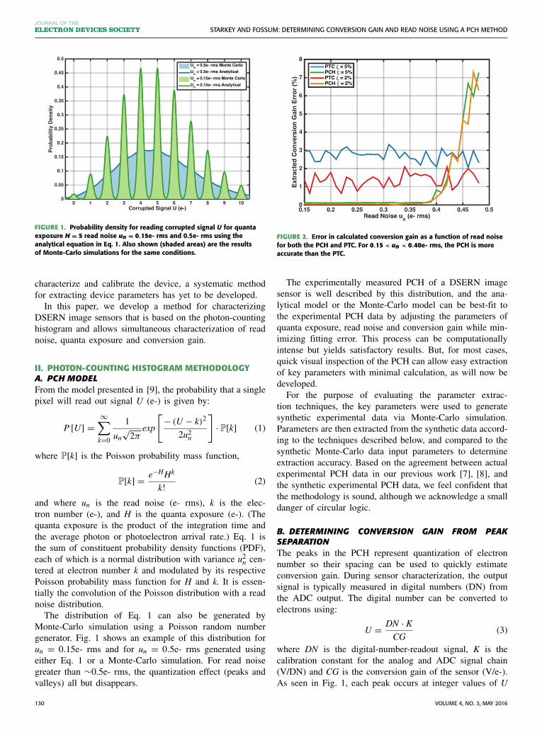
FIGURE 1. Probability density for reading corrupted signal U for quantaexposure H = 5 read noise un = 0.15e- rms and 0.5e- rms using theanalytical equation in Eq. 1. Also shown (shaded areas) are the resultsof Monte-Carlo simulations for the same conditions.

characterize and calibrate the device, a systematic methodfor extracting device parameters has yet to be developed.In this paper, we develop a method for characterizing

DSERN image sensors that is based on the photon-countinghistogram and allows simultaneous characterization of readnoise, quanta exposure and conversion gain.

II. PHOTON-COUNTING HISTOGRAM METHODOLOGYA. PCH MODELFrom the model presented in [9], the probability that a singlepixel will read out signal U (e-) is given by:

P [U] =∞∑

k=0

1

un√

2πexp

[− (U − k)2

2u2n

]· P[k] (1)

where P[k] is the Poisson probability mass function,

P[k] = e−HHk

k!(2)

and where un is the read noise (e- rms), k is the elec-tron number (e-), and H is the quanta exposure (e-). (Thequanta exposure is the product of the integration time andthe average photon or photoelectron arrival rate.) Eq. 1 isthe sum of constituent probability density functions (PDF),each of which is a normal distribution with variance u2

n cen-tered at electron number k and modulated by its respectivePoisson probability mass function for H and k. It is essen-tially the convolution of the Poisson distribution with a readnoise distribution.The distribution of Eq. 1 can also be generated by

Monte-Carlo simulation using a Poisson random numbergenerator. Fig. 1 shows an example of this distribution forun = 0.15e- rms and for un = 0.5e- rms generated usingeither Eq. 1 or a Monte-Carlo simulation. For read noisegreater than ∼0.5e- rms, the quantization effect (peaks andvalleys) all but disappears.

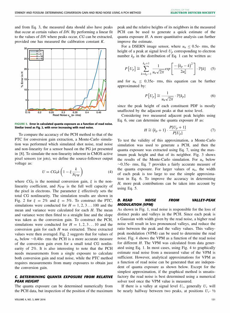
FIGURE 2. Error in calculated conversion gain as a function of read noisefor both the PCH and PTC. For 0.15 < un < 0.40e- rms, the PCH is moreaccurate than the PTC.

The experimentally measured PCH of a DSERN imagesensor is well described by this distribution, and the ana-lytical model or the Monte-Carlo model can be best-fit tothe experimental PCH data by adjusting the parameters ofquanta exposure, read noise and conversion gain while min-imizing fitting error. This process can be computationallyintense but yields satisfactory results. But, for most cases,quick visual inspection of the PCH can allow easy extractionof key parameters with minimal calculation, as will now bedeveloped.For the purpose of evaluating the parameter extrac-

tion techniques, the key parameters were used to generatesynthetic experimental data via Monte-Carlo simulation.Parameters are then extracted from the synthetic data accord-ing to the techniques described below, and compared to thesynthetic Monte-Carlo data input parameters to determineextraction accuracy. Based on the agreement between actualexperimental PCH data in our previous work [7], [8], andthe synthetic experimental PCH data, we feel confident thatthe methodology is sound, although we acknowledge a smalldanger of circular logic.

B. DETERMINING CONVERSION GAIN FROM PEAKSEPARATIONThe peaks in the PCH represent quantization of electronnumber so their spacing can be used to quickly estimateconversion gain. During sensor characterization, the outputsignal is typically measured in digital numbers (DN) fromthe ADC output. The digital number can be converted toelectrons using:

U = DN · KCG

(3)

where DN is the digital-number-readout signal, K is thecalibration constant for the analog and ADC signal chain(V/DN) and CG is the conversion gain of the sensor (V/e-).As seen in Fig. 1, each peak occurs at integer values of U

130 VOLUME 4, NO. 3, MAY 2016

STARKEY AND FOSSUM: DETERMINING CONVERSION GAIN AND READ NOISE USING A PCH METHOD

and from Eq. 3, the measured data should also have peaksthat occur at certain values of DN. By performing a linear fitto the values of DN where peaks occur, CG can be extracted,provided one has measured the calibration constant K.

FIGURE 3. Error in calculated quanta exposure as a function of read noise.Similar trend as Fig. 2, with error increasing with read noise.

To compare the accuracy of the PCH method to that of thePTC for conversion gain extraction, a Monte-Carlo simula-tion was performed which simulated shot noise, read noiseand non-linearity for a sensor based on the PG jot presentedin [8]. To simulate the non-linearity inherent in CMOS activepixel sensors (or jots), we define the source-follower outputvoltage as:

U = CG0k

(1 − ξ

k

NFW

)(4)

where CG0 is the nominal conversion gain, ξ is the non-linearity coefficient, and NFW is the full well capacity ofthe pixel in electrons. The parameter ξ effectively sets thetotal CG nonlinearity. The simulation results are shown inFig. 2 for ξ = 2% and ξ = 5%. To construct the PTC,simulations were conducted for H = 1, 2, 3 . . . 100 and themean and variance were calculated for each H. The meanand variance were then fitted to a straight line and the slopewas taken as the conversion gain. To construct the PCH,simulations were conducted for H = 1, 2, 3 . . . 10 and theconversion gain for each H was extracted. These extractedvalues were then averaged. Fig. 2 suggests that for values ofun below ∼0.40e- rms the PCH is a more accurate measureof the conversion gain even for a small total CG nonlin-earity of 2%. It is also interesting to note that the PCHneeds measurements from a single exposure to calculateboth conversion gain and read noise, while the PTC methodrequires measurements from many exposures to obtain justthe conversion gain.

C. DETERMINING QUANTA EXPOSURE FROM RELATIVEPEAK HEIGHTThe quanta exposure can be determined numerically fromthe PCH data, but inspection of the position of the maximum

peak and the relative heights of its neighbors in the measuredPCH can be used to generate a quick estimate of thequanta exposure H. A more quantitative analysis can furtherimprove the estimate.For a DSERN image sensor, where un ≤ 0.5e- rms, the

height of a peak at signal level Up corresponding to electronnumber kp in the distribution of Eq. 1 can be written as:

P[Up

] ∼=kp+1∑

k=kp−1

1

un√

2πexp

[− (

kp − k)2

2u2n

]· P[k] (5)

and for un ≤ 0.35e- rms, this equation can be furtherapproximated by:

P[Up

] ∼= 1

un√

2π· P[kp] (6)

since the peak height of each constituent PDF is mostlyunaffected by the adjacent peaks at that noise level.Considering two measured adjacent peak heights using

Eq. 6, one can determine the quanta exposure H as:

H ∼= (kp + 1

) · P[Up + 1]

P[Up](7)

To test the validity of this approximation, a Monte-Carlosimulation was used to generate a PCH, and then thequanta exposure was extracted using Eq. 7, using the max-imum peak height and that of its neighbor. Fig. 3 showsthe results of the Monte-Carlo simulation. For un below∼0.35e- rms, Eq. 7 provides a fairly accurate measure ofthe quanta exposure. For larger values of un, the widthof each peak is too large to use the simple approxima-tion in Eq. 6. To improve the accuracy in determiningH, more peak contributions can be taken into account byusing Eq. 5.

D. READ NOISE FROM VALLEY-PEAKMODULATION (VPM)As shown in Fig. 1, read noise is responsible for the loss ofdistinct peaks and valleys in the PCH. Since each peak isa Gaussian with width given by the read noise, a higher readnoise will result in less pronounced valleys, and reduce theratio between the peak and the valley values. This valley-peak modulation (VPM) can be used to determine the readnoise. Fig. 4 shows the VPM as a function of the read noisefor different H. The VPM was calculated from data gener-ated using Eq. 1. In most cases, using Fig. 4 to graphicallyestimate read noise from a measured value of the VPM issufficient. However, analytical approximations for VPM asa function of read noise can be generated that are indepen-dent of quanta exposure as shown below. Except for thesimplest approximation, if the graphical method is unsatis-factory the read noise is best determined using a numericalsolver tool once the VPM value is measured.If there is a valley at signal level Uv, generally Uv will

be nearly halfway between two peaks, at positions Uv- ½

VOLUME 4, NO. 3, MAY 2016 131

STARKEY AND FOSSUM: DETERMINING CONVERSION GAIN AND READ NOISE USING A PCH METHOD

FIGURE 4. VPM as a function of read noise. For un = 0.15e- rms, the valleyprobability is nearly zero, so the VPM goes to 1. As un increases, thevalley-peak ratio approaches 1, so the VPM approaches 0.

and Uv+ ½. Letting kp = Uv− ½ and assuming un < 0.5e-rms, we can write:

P [Uv] ∼=kp+1∑

k=kp

1

un√

2πexp

⎡

⎢⎣−

(kp + 1

2 − k)2

2u2n

⎤

⎥⎦ · P[k] (8)

Note only the peaks at kp and kp+1 are included in thesummation because constituent PDFs further from the val-ley do not have a large influence on the resulting sum.Let PV � P [Uv] (valley PDF value) and let PP �12

{P

[Up

] + P[Up + 1

]}(average of surrounding peak PDF

values). The VPM is defined as:

VPM = 1 − PVPP

(9)

Using the approximations of Eqs. 5 and 8, an approximateexpression for VPM for un < 0.5e- rms is:

VPM ∼= 1 −2 exp

[ −18u2

n

]

1 + β · exp[ −1

2u2n

] (10)

where,

β = P[kp − 1

] + P[kp

] + P[kp + 1

] + P[kp + 2

]

P[kp

] + P[kp + 1

] (11)

If kp and kp+1 are chosen such that they border the centervalley of the PCH then β ∼= 2 (due to the pseudo-symmetryof the PCH so that P

[kp

] − P[kp − 1

] ∼= P[kp + 1

] −P

[kp + 2

], valid for H > ∼5) and an expression independent

of H and kp is obtained:

VPM ∼= 1 −2exp

[ −18u2

n

]

1 + 2exp[ −1

2u2n

] (12)

For un < 0.35e- rms the denominator of Eq. 12 is nearlyunity and:

VPM = 1 − 2exp

[ −1

8u2n

](13)

Another approximation was presented in [7]:

VPM ∼= 1 −2exp

[ −18u2

n

]+ 2exp

[ −98u2

n

]

1 + 2exp[ −1

2u2n

] (14)

which is a result of extending the summation of Eq. 8 toinclude peaks kp-1 and kp+2. Fig. 5 shows a comparisonbetween Eq. 12, 13 and 14.To compare the accuracy of the VPM method to the dark

read noise method, a Monte-Carlo simulation was performedwhich simulated the effects of shot noise and read noise. Forthe dark read noise method H = 0 was used to remove shotnoise from the data. For the VPM method, H = 1, 5 and10 was used to generate a PCH and un was extracted usingEq. 9 and including all peak contributions. The results areshown in Fig. 6. For un < 0.45e- rms, VPM provides a moreaccurate measure of read noise compared to the conventionaldark read noise method.

FIGURE 5. VPM as a function of read noise using Eqs. 12, 13 and 14. Theplot suggests the simple approximation of Eq. 13 does not deviate far fromthe complicated expressions for un < 0.35e- rms.

E. CONVERSION GAIN VARIATION FROM ENSEMBLE PCHSince Eq. 1 applies for a single pixel, the PCH of anarray of pixels will have the same form with an addi-tional source of error due to conversion gain variation.Essentially, the probability that an ensemble of pixels willreadout signal U is:

P [U] =∞∑

k=0

1

σk√

2πexp

[−(U − k)2

2σ 2k

]· P[k] (15)

where

σ 2k = u2

n + k2 (σCG/CG

)2(16)

132 VOLUME 4, NO. 3, MAY 2016

STARKEY AND FOSSUM: DETERMINING CONVERSION GAIN AND READ NOISE USING A PCH METHOD

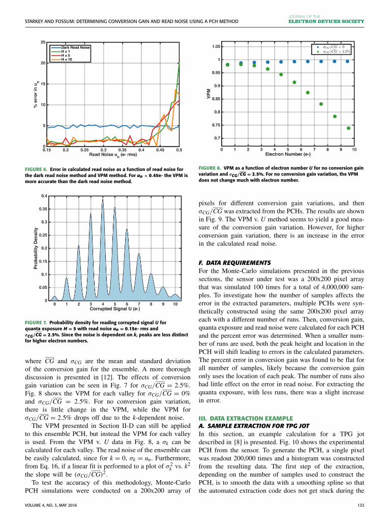
FIGURE 6. Error in calculated read noise as a function of read noise forthe dark read noise method and VPM method. For un < 0.45e- the VPM ismore accurate than the dark read noise method.

FIGURE 7. Probability density for reading corrupted signal U forquanta exposure H = 5 with read noise un = 0.15e- rms andσCG/CG = 2.5%. Since the noise is dependent on k, peaks are less distinctfor higher electron numbers.

where CG and σCG are the mean and standard deviationof the conversion gain for the ensemble. A more thoroughdiscussion is presented in [12]. The effects of conversiongain variation can be seen in Fig. 7 for σCG/CG = 2.5%.Fig. 8 shows the VPM for each valley for σCG/CG = 0%and σCG/CG = 2.5%. For no conversion gain variation,there is little change in the VPM, while the VPM forσCG/CG = 2.5% drops off due to the k-dependent noise.The VPM presented in Section II-D can still be applied

to this ensemble PCH, but instead the VPM for each valleyis used. From the VPM v. U data in Fig. 8, a σk can becalculated for each valley. The read noise of the ensemble canbe easily calculated, since for k = 0, σk = un. Furthermore,from Eq. 16, if a linear fit is performed to a plot of σ 2

k vs. k2

the slope will be (σCG/CG)2.To test the accuracy of this methodology, Monte-Carlo

PCH simulations were conducted on a 200x200 array of

FIGURE 8. VPM as a function of electron number U for no conversion gainvariation and σCG/CG = 2.5%. For no conversion gain variation, the VPMdoes not change much with electron number.

pixels for different conversion gain variations, and thenσCG/CG was extracted from the PCHs. The results are shownin Fig. 9. The VPM v. U method seems to yield a good mea-sure of the conversion gain variation. However, for higherconversion gain variation, there is an increase in the errorin the calculated read noise.

F. DATA REQUIREMENTSFor the Monte-Carlo simulations presented in the previoussections, the sensor under test was a 200x200 pixel arraythat was simulated 100 times for a total of 4,000,000 sam-ples. To investigate how the number of samples affects theerror in the extracted parameters, multiple PCHs were syn-thetically constructed using the same 200x200 pixel arrayeach with a different number of runs. Then, conversion gain,quanta exposure and read noise were calculated for each PCHand the percent error was determined. When a smaller num-ber of runs are used, both the peak height and location in thePCH will shift leading to errors in the calculated parameters.The percent error in conversion gain was found to be flat forall number of samples, likely because the conversion gainonly uses the location of each peak. The number of runs alsohad little effect on the error in read noise. For extracting thequanta exposure, with less runs, there was a slight increasein error.

III. DATA EXTRACTION EXAMPLEA. SAMPLE EXTRACTION FOR TPG JOTIn this section, an example calculation for a TPG jotdescribed in [8] is presented. Fig. 10 shows the experimentalPCH from the sensor. To generate the PCH, a single pixelwas readout 200,000 times and a histogram was constructedfrom the resulting data. The first step of the extraction,depending on the number of samples used to construct thePCH, is to smooth the data with a smoothing spline so thatthe automated extraction code does not get stuck during the

VOLUME 4, NO. 3, MAY 2016 133

STARKEY AND FOSSUM: DETERMINING CONVERSION GAIN AND READ NOISE USING A PCH METHOD

FIGURE 9. Conversion gain variation extraction from synthetic PCHdata using VPM v. U method, showing good agreement between inputparameter and extracted parameter.

FIGURE 10. Sample data from a TPG jot presented in [8]. The experimentaldata and fitted curve show good agreement (see Section III-A for extractedparameters). The peaks and valleys are labeled for reference.

computation. Next, the conversion gain needs to be calcu-lated, so the data can be converted from DN to e-. This isdone by calculating the location and probability of each peakand fitting the location data to a straight line. The result-ing slope is the conversion gain in e-/DN. The value of theconversion gain in µV/e- is obtained by using K, the analogand ADC signal chain calibration constant (see Eq. 3). Forthis example, the extracted conversion gain is 417µV/e-. Thequanta exposure and read noise are not needed to calculatethe conversion gain.Next, the quanta exposure is calculated after the data has

been converted from DN to e-. From Eq. 7 only the peakprobability for kmax and kmax+1 as well as the locationof kmax is needed to determine the quanta exposure. Usingthe peak locations and probabilities calculated in the pre-vious step, the exposure can be calculated resulting ina quanta exposure of 6.87e-.

Finally, the read noise is calculated using the VPM. FromEq. 10 the only additional piece of information needed is thelocation and probability for the valley that is between kmaxand kmax+1. This is straightforward since the location andprobability of the two neighboring peaks is already known.Using Fig. 4, one can simply read off the value of the readnoise based on the VPM. The read noise for this example is0.26e- rms. Alternatively, to calculate the read noise, Eq. 10can be solved for un using a zero finder. Fig. 10 shows thefitted curve overlaid on the original data and illustrates theaccuracy of the extracted parameters.

IV. CONCLUSIONIn this paper, a new method of characterizing DSERNimage sensors is reported based on the photon-countinghistogram (PCH). The accuracy in extracted parameterswas determined using synthetic PCH data. With the pushtowards photon counting image sensors, this method willbe beneficial for characterizing next generation DSERNimage sensors, and has already been successfully used byothers [13].

ACKNOWLEDGMENTThe authors thank TSMC for the fabricating the devices,Augusto Amatori for assisting with Monte-Carlo data gen-eration, and the rest of our group at Dartmouth for providinginsight and feedback.

REFERENCES[1] J. R. Janesick, J. Hynecek, and M. M. Blouke, “Virtual phase imager

for Galileo,” Solid State Imagers Astron., vol. 290, pp. 165–174,Jun. 1981.

[2] L. Mortara and A. Fowler, “Evaluations of charge-coupleddevice (CCD) performance for astronomical use,” in Proc. SPIE,vol. 290. Cambridge, U.K., Jan. 1981, pp. 28–33.

[3] B. P. Beecken and E. R. Fossum, “Determination of the conver-sion gain and the accuracy of its measurement for detector elementsand arrays,” J. Opt. Soc. America, vol. 35, no. 19, pp. 3471–3477,1996.

[4] J. Janesick, K. Klaasen, and T. Elliott, “CCD charge collectionefficiency and the photon transfer technique,” in Proc. 29th Annu.Tech. Symp. Int. Soc. Opt. Photon., San Diego, CA, USA, 1985,pp. 7–19.

[5] N. A. W. Dutton, L. Parmesan, A. J. Holmes, L. A. Grant, andR. K. Henderson, “320×240 oversampled digital single photoncounting image sensor,” in Symp. VLSI Technol. Dig. Tech. Papers,Honolulu, HI, USA, Jun. 2014, pp. 1–2.

[6] J. Ma and E. R. Fossum, “A pump-gate jot device with high conversiongain for a quanta image sensor,” IEEE J. Electron Devices Soc., vol. 3,no. 2, pp. 73–77, Mar. 2015.

[7] J. Ma and E. R. Fossum, “Quanta image sensor jot with sub 0.3e- r.m.s.read noise and photon counting capability,” IEEE Electron DeviceLett., vol. 36, no. 9, pp. 926–928, Sep. 2015.

[8] J. Ma, D. Starkey, A. Rao, K. Odame, and E. R. Fossum,“Characterization of quanta image sensor pump-gate jots with deepsub-electron read noise,” IEEE J. Electron Devices Soc., vol. 3, no. 6,pp. 472–480, Nov. 2015.

[9] E. R. Fossum, “Modeling the performance of single-bit and multi-bitquanta image sensors,” IEEE J. Electron Devices Soc., vol. 1, no. 9,pp. 166–174, Sep. 2013.

[10] P. Finocchiaro et al., “Characterization of a novel 100-channel sili-con photomultiplier—Part II: Charge and time,” IEEE Trans. ElectronDevices, vol. 55, no. 10, pp. 2765–2773, Oct. 2008.

134 VOLUME 4, NO. 3, MAY 2016

STARKEY AND FOSSUM: DETERMINING CONVERSION GAIN AND READ NOISE USING A PCH METHOD

[11] S. Wolfel et al., “Sub-electron noise measurements on RNDR devices,”in Proc. IEEE Nuclear Sci. Symp. Conf. Rec., vol. 1. San Diego, CA,USA, Oct. 2006, pp. 63–69.

[12] E. R. Fossum, “Photon counting error rates in single-bit and multi-bitquanta image sensors,” IEEE J. Electron Devices Soc., to be published.

[13] M.-W. Seo, S. Kawahito, K. Kagawa, and K. Yasutomi, “A 0.27e-rmsread noise 220-µV/e- conversion gain reset-gate-less CMOS imagesensor with 0.11-µm CIS process,” IEEE Electron Device Lett.,vol. 36, no. 12, pp. 1344–1347, Dec. 2015.

DAKOTA A. STARKEY (S’15) received theB.A. degree in physics from Vassar College,Poughkeepsie, NY, USA, in 2013, and the B.E.degree in electrical engineering from DartmouthCollege, Hanover, NH, USA, in 2014, as partof a dual degree program. He is currently pur-suing the Ph.D. degree with the Thayer schoolof Engineering at Dartmouth. His research focusis developing the quanta image sensor (QIS) withemphasis on low-power, high-speed readout circuitdesign, and QIS applications.

ERIC R. FOSSUM (S’80–M’84–SM’91–F’98) iscurrently a Professor with the Thayer Schoolof Engineering at Dartmouth. He is the primaryinventor of the CMOS image sensor used insmartphones and other applications. He is cur-rently exploring the quanta image sensor. Heis the Co-Founder and the Past President ofthe International Image Sensor Society and theDirector of the National Academy of Inventors.He was inducted into the National Inventors Hallof Fame and is a member of the National Academyof Engineering.

VOLUME 4, NO. 3, MAY 2016 135