determing structure-activity relationships between novel ... · determing structure-activity...
TRANSCRIPT

DETERMING STRUCTURE-ACTIVITY RELATIONSHIPS
BETWEEN NOVEL PET RADIOTRACERS AND THEIR NON-
SPECIFIC BINDING PROPERTIES
Chloe Rose Child
A thesis submitted in partial fulfilment of the requirements for the degree
of Doctor of Philosophy
Department of Chemistry
Imperial College of Science Technology and Medicine London
Supervisors: Antony Gee, Nicholas Long and Oscar Ces
February 2012

“Let us run with perseverance the race marked out for us.”
Hebrews 12: 1

i
Declaration
The work described in this thesis was carried out at the Clinical Imaging Centre,
Hammersmith Hospital, London and in the Department of Chemistry, Imperial College
London, from October 2008 to October 2011. The entire body of this work is my own unless
otherwise stated to the contrary and has not been submitted previously for a degree at this or
any other university.
Statement of Copyright
The copyright of this thesis rests with the author. No quotation from it should be used or
published without prior consent of the author and information derived from it should be
acknowledged appropriately.

Abstract
ii
The non-invasive imaging modality positron emission tomography (PET) is used extensively
in clinical settings and is increasingly being used by the pharmaceutical industry in drug
development. Molecules of biological interest are labelled with positron emitting isotopes
e.g. 11
C, allowing their biodistribution and kinetics to be followed in vivo. A major factor in
the failure of radioligands is the magnitude of unwanted background signal, non-specific
binding (NSB) obscuring binding to the desired target. Assumptions have previously been
made as to the physiochemical and pharmacological properties of radioligands that can affect
NSB. However, little work has been carried out to quantify NSB with regard to determining
structure-activity relationships (SARs) in order to optimise efficient radiotracer discovery.
Non-specific binding is a poorly understood process but is believed to be related to the non-
saturable binding of labelled molecules with tissue membranes. In this work the synthesis of
novel radiolabelled molecular libraries has been conducted, their physicochemical properties
determined and their non-specific binding measured in vitro using autoradiographical and cell
based mass spectrometry assay methods. Structure-activity relationships have been formed
between partition coefficient properties, acid dissociation constants, interaction energies and
molecular weight in order to determine the effect each of these properties has on non-specific
binding. Traditionally lipophilicity, log P, of a radioligand is the main predictor to its non-
specific binding properties. However from this work it has been shown that a single
physicochemical property cannot be relied on to predict the NSB of a radioligand but
multiple properties must be considered.

Abbreviations
iii
[11
C]WAY100635 [Carbon-11]-N-(2-(4-(2-methoxyphenyl)-1-piperazinyl)ethyl)-N-(2-
pyridiny)cyclohexanecarboxamide trihydrochloride
[L] Ligand
[R] Receptor
[RL] Receptor-Ligand complex
2D Two dimensional
3D Three dimensional
AS-MS Affinity selection–mass spectrometry
ATP Adenosine triphosphate
B Bound ligand
BBB Blood brain barrier
Bmax Total number of binding sites
BP Binding Potential
C1 Plasma compartment
C2 Intracerebral compartment where tracer is free
C2’ Non-specific binding compartment
C3 Specifically bound compartment
CAD Cationic amphiphilic drug
Ce Cerebellum
CFT Concentration of free ligand in tissue
Ci Curie
CHI Chromatographic hydrophobicity index
CHI_IAM Chromatographic hydrophobicity index of the Immobilised artificial
membrane
CHI_Log D7.4 Chromatographic hydrophobicity index of the distribution partition
coefficient
CHO-K1 Chinese Hamster Ovary cells
CIC Clinical Imaging Centre
CNS Central nervous system
CP Concentration of parent radioligand
CS Concentration of specifically bound ligand
CT Computed Tomography
d Deuteron

Abbreviations
iv
DCRY Decay-corrected radiochemical yield
DMF Dimethylformamide
DMSO Dimethylsulfoxide
DNA Deoxyribonucleic acid
DOPC 1,2-Dioloeyl-sn-glycero-3-phosphocholine
Eint Interaction energy
EOB End of bombardment
ESI-MS Electrospray ionisation mass spectrometry
F Free ligand
GBq Gigabequerels
GSK GlaxoSmithKline
GTP Guanosine triphosphate
HF Hartree-Fock
Hi Hippocampus
HOMO Highest occupied molecular orbital
HPLC High-performance liquid chromatography
HSA Human serum albumin
IAM Immobilised artificial membrane
IC50 Inhibitory concentration
IR Infra-red spectroscopy
IV Intravenous injection
J J-coupling
K Kelvin
Ka Acidity constant
KD Dissociation equilibrium constant
Keq Equilibrium constant
LC/MS Liquid chromatography-mass spectrometry
LiAlH4 Lithium Aluminium hydride
log D Distribution partition coefficient
log P Lipophilicity, partition coefficient
LOR Line-of-response
LUMO Lowest unoccupied molecular orbital
m meta

Abbreviations
v
MALDI-TOF-MS Matrix assisted laser desorption ionisation time-of-flight mass
spectrometry
MBq Mega Becquerel
MC Motor cortex
Me Methyl functional group
Me Meduilla (Chapter 5)
MOPC Mono-oleoylphosphatidylcholine
MS Mass spectrometry
MW Molecular weight
n Neutron
nM Nanomolar
NMR Nuclear Magnetic Resonance
s Singlet
d Doublet
dd Double doublet
ddd Doublet of doublet of doublets
t Triplet
td Triplet of doublets
Hz Hertz
δ Chemical shift
ppm Parts per million
NOE Nuclear Overhauser Effect
NOESY Nuclear Overhauser Effect Spectroscopy
NSB Non-specific binding
NSB % Non-specific binding percentage
o Ortho
p Para
p Proton
P Caudate Putamen
PC Phosphatidylcholine
PET Positron Emission Tomography
pKa Acid dissociation constant
PQX Pyrroloquinoxaline

Abbreviations
vi
R Organyl group
RCP Radiochemical purity
RCY Radiochemical yield
ROI Region of interest
SA Specific Activity
SAR Structure-Activity Relationship
t Triplet
td Triplet of doublets
TEA Triethylamine
Tris Tris(hydroxymethyl)aminoethane
UV Ultraviolet Spectroscopy
VF Volume of distribution of free ligand
VND Volume of distribution of non-displaceable ligand
VNS Volume of distribution of non-specifically bound ligand
VS Volume of distribution of specifically bound ligand
VT Volume of distribution of total ligand

Acknowledgements
vii
Over the last three years of this PhD, this project has proven to be multidisciplinary and
multifaceted and as such, a large number of people have been involved and contributed in
helping to obtain various results.
I would first like to say a huge thank you to Tony Gee, Nick Long and Oscar Ces for giving
me the opportunity to carry out this PhD. I would particularly like to say a massive thank
you for their continued support and encouragement throughout the project as well as direction
during inspirational ruts. I would also like to thank them for the endless reading and editing
of this PhD thesis, without which there would be a much larger number of grammatical errors
present.
A large thank you must go to GSK and all the staff at the CIC at the Hammersmith Hospital,
London for providing an enjoyable working environment and a lab space to work in. I would
like to specially thank Jean-Francois Deprez (Jeff) and Steven Kealey who showed great
patience when teaching me the radiolabelling techniques in the R&D laboratories and helping
solve the numerous problems that arose with various computer programs. I would also like to
thank the rest of the chemistry team at GSK for helping to solve numerous problems and for
all their suggestions when something was not working correctly.
A special thank you must go to Christine Parker at the CIC whose advice and guidance on
cell techniques and the autoradiographical methods carried out in this work was invaluable. I
would also like to thank her for instruction in all things biological, showing me how to use
the biology laboratories at the CIC, and for reading and commenting on several chapters of
this thesis.
This PhD has proven to be extremely multidisciplinary and it has not been possible to carry
out all the data collection alone. I would like to thank Callum Dickson for performing the
interaction energy calculations, Klara Valko for instructing me in lipophilicity partition
coefficients and the HPLC methods used in this work. I also appreciate the work Ian Reid of
GSK, Stevenage carried out measuring the acid dissociation constants of various compounds
used in this work.
I am extremely grateful to Imperial College London for providing a space for me to carry out
my research and also John Barton who provided mass spectrometry data for the compounds
synthesised in this work, and Stephen Boyer at London Metropolitan University who
processed all the elemental analysis data stated in this thesis. A large thank you also goes to

Acknowledgements
viii
GSK and BBSRC who have funded this project and without whom this work would not be
possible.
This project would not have been as enjoyable as it was had it not been for all the members of
the Long research group especially Lucy, Myra, Chris, Jay, Mike, Sheena and Anna in lab
361 at Imperial College and their continuous laughter and numerous distractions. A thank
you must also go to the Membrane Biophysics Group who allowed me to use some of their
lab space particularly Rosa for her help with the CHO-K1 cell work.
Thank you to my husband Peter for his love and support through this PhD and the endless
chemistry discussions he has endured. I would also like to thank my family and friends who
have offered support when the research was not going well and provided me with distractions
from the laboratory. Without all their love and encouragement I know this PhD would have
been a far greater challenge. I would finally like to thank Chirag (Shaggy) who encouraged
me to take on a life of research.
Thanks also go to all those not mentioned here as I am sure there are many I have forgotten.
I have learnt so much through this PhD and have really enjoyed how this project has
developed and changed over the years.

Contents
ix
CONTENTS
Page
Declaration of Originality i
Abstract ii
Abbreviations iii
Acknowledgements vii
1.0 CHAPTER ONE: INTRODUCTION
1.1 The cell and cell membrane 2
1.2 Receptors 4
1.3 Positron Emission Tomography, PET 6
1.3.1 What is PET and how does it work? 6
1.3.2 Common radionuclides, with particular emphasis on carbon-11 9
1.3.3 Advantages and limitations 11
1.3.4 PET in a clinical setting 12
1.3.5 PET in the pharmaceutical industry 14
1.4 PET imaging and receptor-binding 15
1.5 Non-specific Binding, NSB 24
1.6 Structure-Activity Relationships, SARs 32
1.7 Structure-Activity Relationship (SAR) hypotheses 34
1.8 Aims and Objectives 35
1.9 References 36
2.0 CHAPTER TWO: ORGANIC SYNTHESIS
2.1 Introduction 42
2.1.1 Designing compound libraries 42
2.1.2 Designing compounds for investigating non-specific binding 42
2.1.3 The piperazine functional group 43
2.2 Results and Discussion 44
2.2.1 Synthesis of 1-(2-hydroxyphenyl)piperazine derivatives, compounds 1 – 9 45
2.2.2 Synthesis of 1-(2-methoxyphenyl)piperazine derivatives, compounds 10 – 18 50
2.2.3 1H NMR characteristic peaks
53

Contents
x
a) Changes between the hydroxyphenyl and methoxyphenyl compounds in the
aromatic region
53
b) Broadening of the piperazine proton peaks 55
2.3 Experimental 59
2.3.1 General Instructions 59
2.3.2 Synthesis of 1-(2-hydroxyphenyl)piperazine derivatives, 2 – 6 59
a) 1-(2-Hydroxyphenyl)-4-methylpiperazine (2) 60
b) 1-(2-Hydroxyphenyl)-4-propylpiperazine (3) 60
c) 1-(2-Hydroxyphenyl)-4-butylpiperazine (4) 60
d) 1-(2-Hydroxyphenyl)-4-pentylpiperazine (5) 61
e) 1-(2-Hydroxyphenyl)-4-nonalpiperazine (6) 61
f) 1-(2-Hydroxyphenyl)-4-benzyl-piperazine (7) 61
g) 1-(2-Hydroxyphenyl)-4-pyridyl-piperazine (8) 62
h) 1-(2-Hydroxyphenyl)-4-acetyl-piperazine (9) 62
2.3.3 Synthesis of 1-(2-methoxyphenyl)piperazine derivatives, 11 – 15 63
a) 1-(2-Methoyxphenyl)-4-methylpiperazine (11) 63
b) 1-(2-Methoxyphenyl)-4-propylpierazine (12) 63
c) 1-(2-Methoxyphenyl)-4-butylpiperazine (13) 64
d) 1-(2-Methoxyphenyl)-4-pentylpiperazine (14) 64
e) 1-(2-Methoxyphenyl)-4-nonalpiperazine (15) 64
2.3.4 Synthesis of 1-(2-methoxyphenyl)piperazine derivatives, 16 – 18 65
a) 1-(2-Methoxyphenyl)-4-benzyl-piperazine (16) 65
b) 1-(2-Methoxyphenyl)-4-pyridyl-piperazine (17) 66
c) 1-(2-Methoxyphenyl)-4-acetyl-piperazine (18) 66
2.4 References 67
3.0 CHAPTER THREE: PHYSICOCHEMICAL PROPERTIES
3.1 Lipophilicity, partition coefficient 70
3.1.1 What is lipophilicity, Log P? 70
3.1.2 How is lipophilicity measured? 72
3.1.3 Importance of lipophilicity in PET imaging and hypothesis 74
3.1.4 Methodology 75
3.1.5 Results and Discussion 75

Contents
xi
3.1.6 Immobilised artificial membrane, CHI_IAM 80
3.2 Acid dissociation constant, pKa 83
3.2.1 How is pKa measured? 83
3.2.2 The effect of pKa on NSB hypothesis 85
3.2.3 Methodology 85
3.2.4 Results and Discussion 86
3.3 Interaction Energy, Eint 87
3.3.1 Results and Discussion 89
3.4 Molecular weight 91
3.5 Summary of all compounds and their properties 92
3.6 Conclusion 94
3.7 Experimental 94
3.7.1 Lipophilicity measurements, CHI_Log D7.4 at pH 2.2, 7.4 and 10.5 94
3.7.2 Lipophilicity measurements, CHI_IAM 95
3.8 References 96
4.0 CHAPTER FOUR: RADIOSYNTHESIS
4.1 Introduction 100
4.1.1 Radiosynthesis considerations 100
4.1.2 [11
C]methyl iodide, [11
C]CH3I, production 101
4.1.3 Reaction setup: Synthra module – 11
CH3I production 102
4.1.4 Reaction setup: Radiosynthesis and purification of radiotracers 103
4.1.5 Efficiency of [11
C]CH3I in DMF 104
4.2 Results and Discussion 106
4.2.1 Radiolabelling [11
C]18 and caesium carbonate base 107
4.2.2 Purification of radiotracers and quality control 108
4.2.3 Radiochemical yield 112
4.2.4 Radiochemical purity 113
4.2.5 Specific activity 114
4.3 Conclusion 116
4.4 Experimental 117
4.4.1 Synthesis of [11
C]11 – [11
C]14, [11
C]16 and [11
C]17 117
a) General Preparation 117

Contents
xii
b) Synthesis of [11
C]18 117
4.5 References 118
5.0 CHAPTER FIVE: MEASURING NON-SPECIFIC BINDING WITH
AUTORADIOGRAPHY
5.1 Introduction 120
5.2 Methodology 121
5.3 Results and Discussion 125
5.3.1 Time-course experiments 125
5.3.2 Possibility of specific binding 128
5.3.3 Possible receptors to which [11
C]11 and [11
C]16 may bind 132
5.3.4 Non-specific binding % using cerebellum data 134
5.4 Structure-Activity Relationships 136
5.4.1 Lipophilicity, CHI_Log D7.4 137
5.4.2 Immobilised artificial membrane, CHI_IAM 138
5.4.3 Acid dissociation constant, pKa 140
5.4.4 Interaction energy, Eint 141
5.4.5 Molecular weight 143
5.5 Conclusion 144
5.6 Experimental 145
5.6.1 Tissue preparation 145
5.6.2 Autoradiography – General procedure 145
5.6.3 Materials 145
5.6.4 Data analysis 145
5.7 References 146
6.0 CHAPTER SIX: USING MASS SPECTROMETRY TO DETERMINE NSB
% OF COMPOUNDS FROM A CHO-K1 CELL ASSAY
6.1 Introduction 149
6.2 Methodology 153
6.3 Results and Discussion 157
6.3.1 Pilot study 157
6.3.2 CHO-K1 LC-MS/MS using Tris buffer, pH 7.4 159

Contents
xiii
6.3.3 Lipophilicity, CHI_Log D7.4 versus NSB % 160
6.3.4 CHI_IAM versus NSB % 163
6.3.5 Acid dissociation constant, pKa versus NSB % 164
6.3.6 Interaction energy versus NSB % 166
6.3.7 Molecular weight versus NSB % 167
6.4 Comparison between autoradiography NSB % and the mass spectrometry cell
assay NSB %
168
6.5 Conclusion 174
6.6 Experimental 175
6.6.1 Pilot CHO-K1 cell assay 175
6.6.2 Final CHO-K1 cell assay 175
6.7 References 176
7.0 CHAPTER SEVEN: CONCLUSION AND FUTURE WORK
7.1 Conclusion 178
7.2 Future work 182
7.2.1 Development of CHI_IAM as a measure of non-specific binding 182
7.2.2 Specific binding study with compounds [11
C]11 and [11
C]16 183
7.2.3 Development of mass spectrometry cell assay 185
7.2.4 Adaption of a compound with known NSB, proof-of-principle 186
7.2.5 Deuterium (2H) NMR orientation study 188
7.3 References 190

CHAPTER ONE:
INTRODUCTION

Chapter One: Introduction
2
1.0 CHAPTER ONE: INTRODUCTION
1.1 The cell and cell membrane
When a neurotransmitter, hormone or drug molecule is transported around the body to a
target site, it will have to cross the permeable barrier surrounding a cell. The cell is the basic
living structural and functional unit making up the body and is made of characteristic parts
which enable each cell to undertake a unique biochemical and structural role. The cell
contains the nucleus, the brain of the cell, which controls the reproduction of DNA and the
metabolism of the cell, as well as containing the endoplasmic reticulum, ribosome, golgi
apparatus and mitochondria.1
A cell performs various functions including regulating the flow of ions, hormones and other
molecules into the cell. It also carries out the generation of adenosine triphosphate, ATP,
from the breakdown of nutrients, the synthesis of molecules, transportation within and
between cells and waste removal from the cell. The cell is surrounded by a flexible but
sturdy barrier known as the cell membrane which is a selective permeable barrier that
controls the flow of materials across the membrane.
Figure 1: Structure of the cell membrane and the main features including the phospholipids,
cholersterol and proteins. Taken from www.nature.com on 15 November 2011.2
The cell membrane is formed of two back-to-back layers forming a lipid bilayer and consists
of three main components known as phospholipids, cholesterol and glycolipids. The lipid
bilayer is made up of varying quantities of these making it a very complex system. It
contains a non-polar central region surrounded by a polar region facing out towards the
extracellular fluid, and a polar region facing the cytoplasm within the cell. This occurs due to
each phospholipid being amphiphatic in nature with a hydrophilic polar head group and a
hydrophobic non-polar tail.1

Chapter One: Introduction
3
Phospholipids are the primary building block of the cell membrane. The phosphate
hydrophilic polar head group will reside in the aqueous phase, i.e. either the extracellular
fluid outside the cell or the cytoplasm inside the cell, while the fatty acid tail is hydrophobic
and non-polar forming the hydrophobic interior of the lipid bilayer.
A) B)
Figure 2: A) Chemical structure of a phospholipid where R is an alkyl chain of carbon length, Cn, and
B) a cartoon representation of the hydrophilic head group (circle) and the hydrophobic tail (grey line).
The phospholipid tail usually consists of two alkyl chains and depending on the chain length
and conjugation, the overall curvature of the membrane is affected. When placed in an
aqueous solution, phospholipids form micelles or bilayers driven by the hydrophobic effect.
The fatty acid tails bury away from the aqueous phase whilst the polar phosphate head group
forms interactions with the surrounding water.3
Lipids in the cell membrane are highly varied with regards to their head group, chain length
and degree of saturation. In vivo the role of the lipid bilayer extends beyond
compartmentalisation of the internal cell structures. The lipid bilayer is also involved with
signalling pathways and it has the ability to change composition as a response to the external
environment surrounding the cell.4
Embedded within the cell membrane, are integral proteins which extend in and through the
lipid bilayer which are also amphiphathic in nature. If the integral protein extends the entire
bilayer and protrudes from either side it is known as a transmembrane protein. A class of
integral proteins are known as receptors which serve as cellular recognition sites. Various
molecules or signal transmitters will travel across a synapse or intercellular space to bind to

Chapter One: Introduction
4
specific proteins. On binding to the receptor protein a signal is induced and a biological
response observed. The molecule that binds to the receptor is known as a ligand.
1.2 Receptors
The cell membrane is a lipid bilayer made up of different types of phospholipids and contains
proteins known as receptors. A receptor is a binding or recognition component on the surface
of a cell which receives specific chemical signals from neurotransmitters or hormones.5 A
signalling molecule referred to as a ligand (neurotransmitter or hormone) binds to a receptor
sending a signal to a control centre which maintains the system, before passing the signal to
an effector. An effector is the component that receives the signal and initiates a biological
response.1
Figure 3: A cartoon representation of the receptor structure and a ligand binding.
The receptors in the cell membrane can be divided into three classes. These include, G-
protein coupled receptors, ion channels and receptors with a single transmembrane unit,
figure 4. G-proteins interact with GTP-binding proteins and consist of 7-transmembrane
helices. Ion channels are composed of several subunits organised in a ring that forms the
channel containing the receptor binding.6

Chapter One: Introduction
5
Figure 4: The lipid bilayer containing the G-proteins, ion channels and single transmembrane units
(enzyme linked receptor).
For a protein to be termed a receptor it must have a set of properties associated with it. It is
important that the binding of ligands to the receptor is saturable due to there being a finite
number of receptors present in the bilayer. The receptor specificity should be such that the
receptor only responds to a particular type of ligand. It should also be evident that a
correlation between binding affinity of a series of ligands and the biological response exists.
Another characteristic of receptors is their reversibility. It is important that neurotransmitters,
hormones or drug molecules are able to reversibly bind so as to be able to dissociate from the
receptor once an effect has been induced.5
The neurotransmitter, hormone or drug molecule that binds to a receptor is referred to as a
ligand. When a ligand binds to a receptor and activates an effect of a natural endogeneous
neurotransmitter or hormone, it is known as an agonist. If a ligand binds and blocks the
receptor exerting an effect which would otherwise occur, it is known as an antagonist. Drugs
synthesised for particular receptors will act as either agonists or antagonists.
A receptor can bind a ligand leading to activation or blocking of a biological response and it
can mediate this response rapidly or slowly. Fast responding receptors will be activated and
can carry out the biological response rapidly as seen in the nicotinic acetylcholine receptors.
Acetylcholine binds to the receptor and mediates the transport of sodium and potassium ions
across the cell membrane. The structure of fast response receptors consists of oligometric
transmembrane proteins containing both the agonist binding site and ion channels.
Ion Channel Linked
Receptor
G-Protein Linked
Receptor
Enzyme Linked
Receptor
Na+

Chapter One: Introduction
6
Depending on the selectivity of the ion channel contained in the oligomer, activation of the
receptor will be a rapid excitation or inhibitory response.7
Slow responding receptors have a simpler structure consisting of a single polypeptide
containing the receptor site and G-protein acting as a transducer to the effector. These type
of receptors show slower responses and are analogous to the actions of hormones on the cell
surface. Receptors in the periphery and central nervous system are able to couple directly to
ion channels via G-proteins and include examples such as adenosine, muscarinic
acetylcholine and serotonin receptors.7
A ligand can bind to a fast or slow response receptor either as an agonist or antagonist. The
kinetics of these processes can be measured both in vitro and in vivo to quantify specific and
non-specific binding. Positron emission tomography (PET) is an imaging modality utilising
the radionuclides incorporated into radioligands to investigate the binding of ligands to
specific receptors and to quantify features of the binding sites, i.e. the number of binding sites
and affinity of a radioligand.
1.3 Positron Emission Tomography, PET
1.3.1 What is PET and how does it work?
Positron emission tomography (PET) is a non- invasive nuclear imaging technique utilising
the decay characteristics of positron emitting radioisotopes.8 It is used to investigate in vivo
metabolic function, biological processes and target receptor distr ibution in the brain. PET
has found application in the clinical setting allowing the diagnosis of diseases, measure
treatments and their effectiveness. Also, it is increasingly being used in the pharmaceutical
industry during drug development as it offers the potential to visualise target sites, aid in
dosage considerations and observe possible pharmaceutical effects on the human body at a
molecular level.9
PET imaging uses the tracer technique to produce positron emitting tracers with high specific
activities allowing the amount of drug to be administered to a subject to be low, usually less
than 10 nmol and at sub-pharmacological doses. This allows compounds which are toxic or
highly potent to be radiolabelled and administered to living subjects as there are no
pharmacological or toxicological effects. This means it is possible to administer novel drug
molecules at tracer doses and assess them using PET imaging at the early stage of drug
development.10

Chapter One: Introduction
7
Radionuclides are produced using charged particle nuclear reactions in a cyclotron where a
target container holding a gas or a fluid is bombarded with protons or deuterons. Crane and
Lauritsen first showed that carbon-11 could be produced by protons at a 10 % higher level
than when using deuterons. They also showed that the carbon-11 product from B2O3 was a
gas that rapidly diffused out of the B2O3 existing as 11CO or 11CO2.11
Today, radionuclides are produced in a cyclotron which accelerates charged particles to high
energies before bombarding stable atoms to produce radioisotopes.9 A high energy beam of
charged particles (protons, deuterons, helium-3 or helium-4), collide with target nucleus
atoms forming the radioactive isotope.12 Generally a proton beam is used in the accelerator
which travels through the target material (the liquid or gas) to undergo nuclear
transformation, forming a precursor which can be used directly or converted into other
precursors for further synthesis and incorporation into drug compounds.
Cyclotrons have the benefit of dual beam capabilities allowing simultaneous bombardments
to be carried out. They also have the advantage of being self-shielding by the addition of a
steel frame and hydraulically driven movable blocks made of concrete to offer complete
radiation protection without the need for large concrete vaults. The control and automation
of a cyclotron by PC and low maintenance requirements has also made them more user
friendly and cheaper to run.12
Table 1 shows the most common radionuclides produced in the cyclotron, their target
material if known, the nuclear reaction undertaken during bombardment and their most
common chemical forms.
Radionuclide Target Material Nuclear Reaction Chemical Form
Carbon-11 14N2 + 16O2 (1%) 14N(p,α)11C 11CO2 or 11CH4
Nitrogen-13 5 mM ethanol in
sterile water
16O(p,α)13N 13NH4+ or 13NOx
Oxygen-15
15N2 + 16O2
15N(p,n)15O
14N(d,n)15O
15O2
Fluorine-18 H218O or 18O2 18O(p,n)18F 18F- or 18F2
Table 1: The main radionuclides used in PET imaging produced in the cyclotron, the target material
used, the nuclear reaction and chemical form of the final precursor (p = proton, n = neutron and d =
deuteron).12, 13

Chapter One: Introduction
8
After the radionuclide has been produced in the cyclotron it is incorporated into a compound
of interest before being introduced into a body at the nanomolar scale, usually by intravenous
(IV) injection. At the target site or region of interest (ROI), the radioligand decays producing
positrons which move through the cellular tissue losing its kinetic energy due to inelastic
interactions with electrons in the tissue. After 10-1 to 10-2 cm, the majority of the positron’s
kinetic energy will have dissipated and it will combine with an electron forming a hydrogen-
like positronium. An annihilation process will then occur and the mass of the particle will be
converted to electromagnetic energy releasing two emissions of high energy photons (511
keV each) at 180o degrees to one another known as line-of-response (LOR), figure 5.8
Figure 5: The annihilation of a positron (β+) and an electron (β-) during PET imaging.
The photons produced during the annihilation process are very energetic which gives the
radiation a high chance of escaping the body for detection externally. The LOR of the
photons also allows for easy detection and localisation which will indicate where the point of
annihiliation is and indicate the position of the radioactive atom in the body.
Figure 6: The PET scanner and line-of-response (LOR) being detected. Image taken from Zi et al.14

Chapter One: Introduction
9
It is important in the production of radionculides to obtain high specific activities from the
cyclotron production. Specific activity of a radionuclide is a measure of the radioactivity per
unit mass of the labelled compound commonly expressed as giga-becquerel per micromole
(GBq/µmol).15 High specific activities are important so that when the radionuclide is
incorporated in the radiotracer, only small mass amounts are used to probe the physiological
process in order not to perturb the process. With a high specific activity, small amounts of
radiotracer can be injected but a strong radiation signal can be detected. This makes PET a
tracer technique and allows investigations to be carried out at sub-pharmacological doses.13
PET is a quantitative imaging technique that allows the measurement of the regional
concentration of the radiotracer under investigation. Regions of interest (ROIs) are drawn
using computational methods and co-registration with other imaging modalities such as
computed tomography (CT).14
1.3.2 Common radionuclides, with particular emphasis on carbon-11
Carbon-11, nitrogen-13, oxygen-15 and fluorine-18 are the most commonly used cyclotron
produced radionuclides in PET imaging. These imaging probes have short half- lives with
carbon-11 (t1/2 = 20.4 min), nitrogen-13 (t1/2 = 9.9 min), oxygen-15 (t1/2 = 2.1 min) and
fluorine-18 (t1/2 = 109.7 min) 16 and as such production, synthesis, purification,
administration and imaging must be undertaken in the shortest period possible, preferably no
longer than 2-3 half lives. These radionuclides are also isotopes of biologically ubiquitous
elements. Most drugs or endogenous compounds are made up of carbon, nitrogen and
oxygen, therefore it is possible to label all drugs or endogenous compounds with a positron
emitter homologous to the non-radioactive counterpart.
Fluorine-18 is an exception as it is not often found in biological compounds however it is
frequently used in radiolabelling as it can sometimes be incorporated into a molecule without
causing too much effect on the pharmacological and physiochemical properties in
comparison to the parent molecule.
Where carbon-11 is the radionuclide of choice, as in this work, it can be produced by
bombarding proton particles with nitrogen-14 in the presence of trace amounts of O2 (1-2 %)
producing 11CO2. For 11CH4, instead of oxygen added to the nitrogen gas, 5-10 % hydrogen
is added to the nitrogen target.17 11CO2 is the main synthon used in all radiosynthesis
reactions however 11CH4 can theoretically give higher specific activities as there is less

Chapter One: Introduction
10
natural methane present in the air to contaminate the radionuclide compared to natural CO 2 in
the air. It is important in order to increase the specific activities of the carbon-11, to exclude
air from synthesis modules and solutions which 11CO2 is initially bubbled through.
Crane and Lauritsen made carbon-11 in 1934 and investigated its physical properties
demonstrating that it decayed by positron emission to the stable 11B atom.11 Carbon-11 has
favourable properties such as a short half- life (t1/2 = 20.4 min, 98.1 % by β+ emission, 1.9 %
by electron capture)18 making it a good labelling radionuclide in medical applications. High
specific activities (10 Ci/µmol)19 are possible meaning decay products can be disregarded
with respect to any biological relevance. Both 11CO2 and 11CH4 once obtained in the
cyclotron can be converted into various secondary precursors leading to an array of possible
synthesises, figure 7. Another advantage of using carbon-11 in PET imaging is the short
half- life of the radioisotope which provides the ability to repeat studies and undertake
multiple scans in one day leading to reduced inter-subject variability.
Figure 7: The commonly produced secondary precursors obtained from 11
CO2 produced in the
cyclotron.19, 20
Carbon-11 is a popular radionuclide to use in the synthesis of PET tracers due to its short
half- life reducing radiation exposure to a subject imaged.21 It also allows for multiple scans
to be carried out on the same day as less time is required between sessions due to the rapid
decay of the radioisotope. However, the short half- life means that carbon-11 can only be
utilised if there is the presence of an on-site cyclotron. Cabon-11 has the ability to produce
large quantities of various synthons including [11C]CH3I, [11C]CO2, [11C]CO and many more,
providing a wide range of synthetic methods available to produce a variety of

Chapter One: Introduction
11
radiopharmecuticals.22, 23 Finally, high specific activities of carbon-11 are possible which are
ideal for PET imaging.
1.3.3 Advantages and limitations
PET offers several advantages as an imaging modality including having a good resolution
and high sensitivity.24 It also allows for the accurate quantification of biological processes
and due to the picomolar concentrations used, this can be carried out without perturbing the
system.14
The biological radionuclides carbon-11, nitrogen-13 and oxygen-15 allow for the synthesis of
radiolabelled compounds indistinguishable from their non-radioactive counter-parts. This
means the biological process should not be affected by the isotopic exchange and the
pharmacological properties of the radiolabelled molecules will be unaffected.24 The shorter
half- life means a subject and staff members receive a lower radiation dose due to the reduced
exposure to radioactive material.
Practically, the development of miniaturised self-shielding cabinets (hot-cells) and low
energy proton cyclotrons has allowed for more centres to have on-site cyclotrons opening up
the possibility for the production of more types of short- lived radioisotopes. The use of
computerised systems installed in hot-cells for automation of the reaction synthesis has also
made the whole process safer for users.9, 16
PET imaging has several advantages and is being used both clinically and in industry.
However it does have its limitations one of which is also one of PET’s major advantages.
The short half- life of the radioisotopes requires production, synthesis, purification, quality
control and image acquisition be carried out as rapidly as possible, ideally between 2 – 3 half-
lives of the chosen radioisotope.
Fluorine-18 has a half- life of 109 minutes and can be made at off-site locations and delivered
to hospitals and research centres when required. However, carbon-11, nitrogen-13 and
oxygen-15 due to their short half- lives require an on-site cyclotron for production. The
development of cyclotron technology has made this more possible, but on-site cyclotrons can
be very expensive to operate. It also requires a specialist team to control and maintain the
cyclotron within a research centre or hospital.

Chapter One: Introduction
12
Another limitation of PET imaging is the need to use radioactive isotopes that produce
gamma radiation. The attenuation of radiation in the body can be damaging to tissue and
cells.
Each imaging modality has its limitations and PET is no exception, however its benefits and
ability to image non- invasively in vivo providing information on biological processes in the
body have made PET an important imaging modality both clinically and industrially.
1.3.4 PET in a clinical setting
There are many different applications that utilise PET imaging including drug development,
medical research and medical diagnosis. Clinically there are three main areas of use for this
technique; neuropsychiatry, cardiology and oncology.
PET imaging and tracers designed for particular targets is being used to improve a clinician’s
ability to assess and diagnose a patient’s disease and track the progression of therapy
adopted. This has seen improved outcomes for patients with earlier detection and better
treatment aimed to be patient-specific.23
PET imaging in neuropsychiatry offers the ability to study and gain a greater understanding
of the brain and its functions. This imaging modality has benefitted such disease diagnosis
and treatment of degenerative dementias (Alzheimer’s), trauma, epilepsy and movement
disorders (Parkinson’s disease).25 A wide range of carbon-11 and fluorine-18 radiotracers
have been radiosynthesised for specific receptor proteins in order to study how each disease
effects certain receptor types and possible therapies that could help cure the disease or relieve
the symptons.24
An example of a radiotracer used in brain imaging is known as [11C]WAY100635, figure 8.
It binds with high affinity and selectivity to 5HT1A receptors in the brain which have been
associated with neuropsychiatic disorders such as anxiety, depression and schizophrenia.
[11C]WAY100635 is increasingly being used to examine the pathophysiology and treatment
of these types of neuropsychiatic disorders giving a better understanding of the disease
progression and the effect of treatments on a patient.26, 27 It is also being used to study the D4
receptors which are associated with modulating cognitive processes and found in the
hippocampus and prefrontal cortex.28

Chapter One: Introduction
13
Figure 8: Chemical structure of [11
C]WAY100635
In cardiology, PET imaging can be used to measure myocardial blood flow using
[13N]ammonia, and [11C]acetate can be used to study the myocardial oxygen consumption in
the heart.19 PET is the only imaging modality that provides non-invasive quantification of
regional tissue perfusion and the oxidation and consumption of O2 in the myocardium as well
as playing a role in the diagnosis and prognosis of coronary heart disease.
PET is widely used in oncology utilising [18F]FDG which is the most common radiotracer
administered to patients for the detection of tumours and metastases, measurement of tumour
progression and impact of treatments administered. The use of [18F]FDG in whole body
imaging allows for tumour staging with high diagnostic accuracy and can be used to
investigate a range of cancers including lymphomas, tumours, colorectal cancer and breast
cancer. PET has improved cancer management of patients and made it possible to provide
patient-specific care.23
[18F]FDG is a glucose derivative and the most commonly used radiotracer in clinical
imaging. It is taken into cells in a similar fashion to glucose and forms a [18F]FDG-6-
phosphate compound which is unable to exit the cell. It accumulates in the cell and the
concentration of this accumulation is directly related to the energetic metabolism in cells. As
such, tumours which have a higher energetic metabolism than healthy cells are highlighted
clearly in the PET image.29
In non-Hodgkin’s lymphoma PET is used to determine that stage of the disease and
determine the best route of treatment whether it is early stage and only radiation treatments
are required, or if it is later stage when lymphoma and systematic therapies are required.30

Chapter One: Introduction
14
1.3.5 PET in the pharmaceutical industry
The discovery and development of new drugs is expensive and time consuming. Generally to
take a drug from the discovery of a new molecule to obtaining regulatory approval and
releasing it on the market can take between 10 – 12 years costing around US$800 million per
drug.22, 31 During the development process many compounds will be abandoned due to safety
issues (too toxic to humans and animals), efficacy (too low activity for target site) or
economics (no commercial market at the end).32
PET is increasingly being used in the pharmaceutical industry for drug development as it can
be used to confirm a drug’s mechanism of action, especially showing the uptake into the
brain, assessment of the kinetics of a new drug and metabolism can also be investigated.33
Initially a target site is identified, either an enzyme, protein receptor or a biomolecule that has
a high affinity binding to a radiotracer. Ligands (compounds that bind to a specific target
site) are designed on the basis of structural biology or using high-throughput screening of
libraries of compounds. Lead compounds or ligands can be identified, optimized and
assessed using PET imaging.34
In drug development, PET is usually applied to biodistribution or receptor occupancy studies.
In biodistribution studies drugs under investigation are radiolabelled directly and PET is used
to study the uptake and delivery to the target site. The concentratio n in tissue can then be
measured quantitatively and an understanding of the drug’s uptake and binding can be
observed.35 Biodistribution studies can be carried out early in the development giving clear
information about the drug’s potential before making large time commitments to further
development.10
Receptor occupancy studies involve labelling a target with a radiotracer which binds
specifically forming a radiotracer-target complex. The radiotracer is then blocked by the
addition of a high concentration of unlabelled drug with specificity for the same target and
observing with PET the blocking of the radioligand. This type of PET study can aid with
quantifying a relationship between the dose of a drug or concentration in plasma with the
occupancy of the drug at a specific target.35

Chapter One: Introduction
15
Studies of the pharmokinetics and biodistribution of new novel drugs are critical in the drug
development process.36 PET imaging is increasingly being used to aid in these studies and
provide information on occupancy distribution, dosing, and the kinetics of new drug
molecules earlier in the development process helping to save time and money.
1.4 PET imaging and receptor-binding
The formation of a ligand-receptor complex is the first step in inducing a biological
response.37 This interaction can be characterised and the number of ligands bound to the
receptor can be measured. PET imaging and radiolabelled ligands can be used to provide
information on the accumulation of a specific radioligand and obtain quantitative information
about the distribution of the target receptor.38
In vitro measures of receptor binding are carried out in multiple ways. One method involves
using an increasing amount of radiolabelled derivative of the ligand under investigation to
give information from direct binding to the receptor. The second method involves measuring
the ability of a non-radiolabelled ligand to block the binding of a high affinity radioligand.
This method involves using a constant concentration of radioligand and increasing the
amount of unlabelled ligand, measuring the radioactivity present in the sample at each
concentration.39, 40
In vitro experiments use radioligands to characterise specific drug binding sites of receptors
in the central nervous system (CNS). The in vitro model is based on the equilibrium reaction
between receptors [R] and ligands [L] to form a receptor- ligand [RL] complex with rate
constants kon and koff (sometimes referred to as k+1 and k-1).41
From the equilibrium reaction the dissociation equilibrium constant, KD, which represents the
amount of ligand that saturates 50 % of the binding sites, can be determined.
= koff
kon = [ ]

Chapter One: Introduction
16
Saturation of the receptor sites occurs at high concentrations of the radioligand (when
concentration >10 x KD) and can be used to calculate the total number of binding sites, Bmax.
[ ]= [ ] ma
[ ]+
The binding potential (BP) can also be calculated and was initially based on the in vitro
radioligand binding and defined as the ratio of Bmax to KD, where the equilibrium dissociation
constant KD is equal to the inverse of the affinity of the ligand binding.42
P = ma
= ma 1
= ma affinity
The Michaelis-Menten equation can be used to describe the in vitro receptor binding at
equilibrium where B is the concentration of receptor bound ligand, Bmax is the density of
receptors, KD is the dissociation constant and F is the concentration of free ligand.
= ma
+
When low mass dose studies are carried out as in PET imaging studies, the concentration of
the free ligand is much lower than the KD and as such the ratio of the receptor-bound ligand
(B) and free ligand (F) can give the binding potential.
=
ma
= P
This means that at tracer levels BP is equal to the equilibrium ratio of the specifically bound
ligand (B) and free ligand (F).41
In vivo studies of binding potential (BP) seek to measure the target receptor in terms of
specific radioligand binding where specific binding is defined as that associated with the
target and distinct from the free and non-specifically bound ligand. These type of studies
require the administration of radioligands at tracer dose in order that the occupancy of
receptor sites is a negilable percentage of the total available receptors but reflects the entire
population.41
In vivo imaging models use multiple compartment models whereas in vitro studies use
models containing only one compartment. This means that the BP from in vitro studies needs
to be converted for in vivo studies. This is achieved by converting B into the concentration of

Chapter One: Introduction
17
specifically bound ligand, CS, and F into the concentration of free ligand in tissue, CFT and
Bmax is referred to as Bavail as only a subset of binding sites are available for binding due to
some being occupied by endogeneous transmitters.
=
T
= avail
= P
The in vivo quantification of receptors can be carried out using a kinetic model known as the
compartment model. The compartment model is based on using compartments to represent
different environments in which a drug can exist. A compartment is a physiological or
biological space where a radiotracer concentration is homogeneous at all times [C(t)]. The
model relies on the assumption that a ligand enters and leaves the plasma and tissue
compartments (crossing the blood-brain barrier) via passive diffusion.38, 40, 43
The 4-compartment model, figure 9, contains a plasma compartment (C1), intracerebral
compartment where tracer is free (C2), a non-specific binding compartment (C2’) and a
specifically bound compartment (C3) with rate constants K1 to k6. K1 describes the transfer of
radiotracer from the plasma (C1) to the tissue (C2) across the blood-brain barrier, and k2-k6
are transfer constants describing the movement between tissue compartments.44
Figure 9: The 4-compartment model representing the plasma compartment (C1), the intracerebral
compartment where tracer is free (C2), the non-specific binding compartment (C2’) and the specific
binding compartment (C3).
C1
C2’
C3 C
2
k6 k
5
k4
k3
k2
K1

Chapter One: Introduction
18
In this compartment model, the assumptions that the volume of distribution (VT) of free and
non-specifically bound ligand are the same in both compartments. The volume of
distribution equals the ratio at equilibrium of each concentration to that of the parent
radioligand (Cp) in plasma separated from radiometabolites. The 4-compartment model is a
robust model however it does lead to imprecise estimates of the parameters being measured.45
The complexity of a 4-compartment model using 6 rate constants makes it difficult to
implement in PET studies. However, if the assumption that the free and non-specific binding
concentrations (C2 and C2’) equilibrate rapidly, k5 and k6 will be high compared to K1 and k2.
This means that compartments C2 and C2’ can be considered one compartment, forming a 3-
compartment model, figure 10.
Figure 10: The 3-compartment model representing the plasma compartment (C1), the free ligand and
non-specific binding compartment (C2) and the specific binding compartment (C3).
In the 3-comparment model, the free ligand and non-specifically bound compartment kinetics
are rapid compared to the specific binding kinetics and as tracers pass in or out of the free
state in the brain, the equilibrium ratio between free and NSB ligand is assumed to be
instantaneously restored.38
A similar 2-compartment model can be adopted if the binding and release of a ligand from
the specific binding compartment is rapid compared to the transport of parameters K1 and k2
giving a single tissue compartment containing free, non-specifically bound and specifically
bound ligand in one compartment.46 Generally though the 3-compartment model is the most
widely used and has been since it was first proposed and used by Mintun et al. 42 in 1984.
Mintun et al.42 proposed the first in vivo method for quantitatively characterising regional
drug binding studies using PET by using a 3-compartment model. Two compartments are
made up of the brain tissue and blood, while a third is formed of the chemical environment
under investigation. In this model it is assumed that all compartments are homogeneous in
concentration and the quantity of drug free to diffuse or react with binding sites is represented
C1 C
3 C
2
k4
k3
k2
K1

Chapter One: Introduction
19
by the total drug concentration multiplied by a constant known as the free fraction, fi. This
term, fi, is in effect the partition of labelled molecules between blood plasma proteins and the
aqueous plasma compartment.
The volume of distribution is also an important parameter to obtain from in vivo PET studies.
The volume of distribution, VT , refers to the total volume of ligand uptake relative to the
concentration of ligand present in the plasma measured in mLcm-3. The target region is
regarded as an organ rather than an entire body and the amount of drug in the entire target is
expressed as an amount of radioligand in a volume of tissue. Tissues may contain
radioligand that is specifically bound to receptors (VS), non-specifically bound (VNS) or free
in tissue water (VF). The volume of distribution of non-displaceable ligand relative to the
total concentration of ligand in plasma (VND) is the sum of the non-specifically bound and
free components.
VT = VS + VNS + VF = VS + VND (where VND = VNS + VF)
This allows specific binding to be calculated from the non-displaceable volume of
distribution by subtracting from the total volume of distribution.
Specific binding (VS) = VT - VND
The benefit of using these types of compartment models is the ability to calculate various
different parameters as described directly from brain data using a variety of reference tissue
regions. This means the need to obtain arterial plasma measurements is not required and can
be a major benefit to a subject being imaged as an invasive arterial cannulation is not required
for the PET scan to be carried out.45, 47
There are various graphical methods that can be used to obtain binding data from PET
imaging assays. These are saturation binding which can be used to obtain KD and Bmax,
competitive binding giving IC50 values, internalisation and efflux.48
Saturation binding measures the specific receptor-mediated uptake of a radiolabelled ligand
of interest at equilibrium with increasing radioligand concentration. This type of experiment
is used to determine the equilibrium dissociation constant, KD, and the total number of
receptors expressed, Bmax. The KD is an important parameter to determine as it can indicate
whether a radioligand has a high or low affinity for a receptor type. If KD is low, the

Chapter One: Introduction
20
radiolgand will have a high affinity while high KD values suggest a radioligand has low
affinity.
During this experiment, either the amount of radioligand is added while keeping a constant
specific activity, or a constant concentration of radioligand is used and the specific activity is
reduced by adding unlabelled ligand. Non-specific binding is then determined at each
concentration by the co- incubation of cells/tissue sections with a 1000-fold excess of the
unlabelled ligand over the KD.49 The specific binding is determined from subtracting the
non-specific binding from the total binding and is plotted against the concentration of the
radioligand producing a saturation curve, figure 11.
Figure 11: Saturation binding curve showing the effect of radioligand concentration (free) on specific
binding (bound).
The saturation binding data can also be represented using a Scatchard plot 37, 50 where the
bound (B) ligand is plotted against the ratio of bound (B) and free (F) ligand. This obtains a
linear relationship and the intercept on the x-axis gives the Bmax value while the gradient of
the line is equal to the inverse of the dissociation constant, KD.

Chapter One: Introduction
21
Figure 12: A Scatchard Plot showing the bound ligand against the B/F ratio and the Bmax and KD
values.
Competitive binding studies are used to determine the concentration of the ligand of interest
required to reduce the specific binding of a radiolabelled standard by 50 % which is known as
the inhibitory concentration, IC50. When the KD is known for a particular radioligand, this
type of study can be used to determine the ability of other unlabelled compounds (over a wide
range of concentrations) to compete for binding of a radioligand of a fixed concentration.49
The lower the IC50 value, the higher the in vitro receptor binding affinity since a lower
concentration of ligand is required to compete with the high affinity radiolabelled standard
for receptor sites. This means IC50 values can be used to compare a series of ligands and
relative receptor binding affinities can be identified. The total binding in the absence of a
competitor is plotted against the Log [competing ligand] generating the IC50 curve forming a
sigmoid curve shape, figure 13.

Chapter One: Introduction
22
Figure 13: Competitive binding curve showing the IC50 (midway between the high and low points of
the curve) and the effect of the competitor concentration on inhibition of the radioligand binding.
Internalisation studies are used to measure receptor-mediated radioligand uptake in cells.
This method is only suitable for studying agonist ligands where the receptor-binding event
signals the cell to internalise the receptor along with the bound radioligand. This method is
useful for obtaining data on the amount and rate of radioligand taken into cells and it can
show whether a large amount of radioligand has been taken up into cells rapidly in vitro,
indicating a potentially efficient in vivo drug delivery system.48
Efflux studies are used to measure the release of internalised radioligand from cells. The
amount and rate at which the agonist radioligand is removed from the cell is recorded and can
provide information regarding the retention of the radioligand. A rapid loss of radioligand
from cells would indicate low in vivo target site retention while a slow loss of radioligand
would suggest a longer period of retention.
There are many different methodologies available to obtain quantitative data from PET
imaging studies. Methods for obtaining this type of data should be chosen in respect to the
information required by the person running the assay. Within the literature there can be slight
variations in the definitions of various parameters, a problem addressed by Innis et al.41 when
they published a review defining the nomenclature for in vivo imaging to help improve the
consistency of data published and remove inconsistencies in definitions of each term used.

Chapter One: Introduction
23
The design and development of potential central nervous system (CNS) candidate
radioligands are usually driven by a general set of criteria for receptor imaging. These
include;51, 52
The ability to penetrate the blood-brain barrier (BBB);
High affinity to target region (high Bmax/KD) to ensure good signal-to-noise ratio;
Selectivity for binding to the target versus non-target sites;
Radioactive metabolites should be hydrophilic showing little uptake in the brain as
radioactive metabolites could increase the non-specific binding component;
Radiolabelling with a positron emitter with high specific radioactivities;
Low non-specific binding.
PET radioligands are usually small drug like molecules crossing the blood-brain barrier via
passive diffusion. This involves transporting the radioligand across the lipid bilayer by
moving from one area of high concentration in the plasma to an area of low concentration in
the brain tissue, requiring no energy to be added to the system. Ideally compounds with the
ability to form very few hydrogen bonds and a molecular weight below 500 Da will lead to
the highest rates of passive diffusion.53, 54
When determining a compound to investigate for affinity to a particular target receptor
protein, large screening libraries of molecules are used to suggest potential lead compounds
for development. Previously four parameters have been suggested to help with the screening
process and indicate which lead molecules have the greatest chance of success. Lipiniski et
al.55 suggested the rule-of- five which is a set of chemical properties that belong to the most
successful pharmaceutical drugs. These state that a compound should have:
1) Less than 5 H-donors in the molecule (sum of OHs and NHs);
2) Molecular weight should be below 500 Da;
3) Lipophilicity, Log P, should be less than 5;
4) There should be less than 10 H-bond acceptors (sum of Os and Ns).
When a molecule has these properties it is likely that it will have the potential to be a drug
molecule with good absorption and permeability in vivo. Antibiotics, antifungals and
vitamins however are a set of molecules that do not follow these rules.55

Chapter One: Introduction
24
1.5 Non-specific Binding, NSB
Positron emission tomography (PET) is increasingly being used in the pharmaceutical
industry to aid in drug development. It can be used to determine a drug’s affinity for a target
site, the assessment of a drug’s kinetics, metabolites can be studied and its potential as a
suitable radiotracer in vitro and in vivo can be evaluated. However, one of the major
contributing factors in the failure of radioligands in PET imaging is it having high non-
specific binding in vivo.
In 1985 Mendel and Mendel published a review claiming that defining non-specific binding
(NSB) as all binding that is non-displaceable by an excess of unlabelled ligand was
inaccurate. This definition would result in an overestimation of the number of high-affinity
receptors and underestimation of the affinity of a given hormone. It is claimed that the
assumption that NSB is non-displaceable is incorrect due it being demonstrated that binding
of labelled hormones to membranes devoid of receptors and inert materials was displaceable.
It is suggested by Mendel and Mendel that some systems can rely on NSB being described as
non-displaceable however the total binding should be measured and appropriate calculations
made and fitted to non-linear regression curves to obtain accurate NSB values.56
The most important point for non-specific binding is to provide a clear definition of the term
in order to remove misinterpretation of this type of binding seen in vitro and in vivo. Non-
specific binding has been previously defined as the binding of radioligands interacting with
macromolecules in tissue other than their intended specific target.52 This definition suggests
that radioligands that bind to receptors other than the target site, make up part of the non-
specific binding component. However it could be argued that the receptors have a finite
number and are saturable so could lead to undesired specific binding rather than non-specific
binding. This does not clearly indicate the classification of non-specific binding.
More commonly, non-specific binding (NSB) is defined as the binding of a radioligand to
non-saturable components in tissue obscuring the visualisation of biological processes under
investigation.15, 57, 58 Non-specific binding is a poorly understood phenomenon in PET
imaging and it is vital that a clear and concise definition is provided by an author. This is to
clearly show which component in the PET image is considered NSB and indicate how it has
been measured. In this work the definition of NSB will follow that as given by Miller et al.15
which states, “non-specific binding is the binding of a labelled compound to a non-saturable
component in tissue.”

Chapter One: Introduction
25
Figure 14: Rat tissue autoradiography showing specific binding (A) and non-specific binding (B) after
blocking with high concentration of unlabelled compound, taken from Kügler et al.59
It can be seen in figure 14 that the rat autoradiography image (A) shows the specific binding
of a [18F]radioligand which has then been displaced using an unlabelled ligand to block all
specific binding. This leaves only non-specifically bound radioligand (B) that is non-
saturable bound to be detected.
In vitro studies of non-specific binding involve measuring NSB using a large excess
concentration of an unlabelled ligand which has affinity for the target site. Initially, a low
concentration of radioligand (subpharmacological dose) with affinity for a target site is
incubated with a tissue sample until equilibrium is reached. The radioactivity in the sample is
measured to obtain the total radioactivity bound, both specifically and non-specifically.
Following this, a high concentration (at least a 100-fold greater) of either the unlabelled
derivative or an unlabelled ligand with high affinity for the target is added. Due to the high
concentration the unlabelled ligand displaces any radioligand specifically bound and the
radioactivity detected on the sample is considered to be non-specifically bound. Subtracting
the NSB radioactivity after blocking with unlabelled ligand from the total radioactivity
measured will give an in vitro measure of specific binding.
Chapter One: Introduction
26
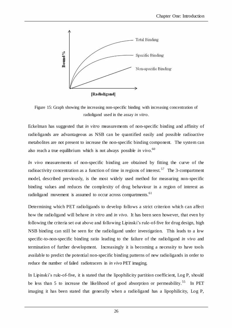
Figure 15: Graph showing the increasing non-specific binding with increasing concentration of
radioligand used in the assay in vitro.
Eckelman has suggested that in vitro measurements of non-specific binding and affinity of
radioligands are advantageous as NSB can be quantified easily and possible radioactive
metabolites are not present to increase the non-specific binding component. The system can
also reach a true equilibrium which is not always possible in vivo.60
In vivo measurements of non-specific binding are obtained by fitting the curve of the
radioactivity concentration as a function of time in regions of interest.57 The 3-compartment
model, described previously, is the most widely used method for measuring non-specific
binding values and reduces the complexity of drug behaviour in a region of interest as
radioligand movement is assumed to occur across compartments.61
Determining which PET radioligands to develop follows a strict criterion which can affect
how the radioligand will behave in vitro and in vivo. It has been seen however, that even by
following the criteria set out above and following ipinski’s rule-of-five for drug design, high
NSB binding can still be seen for the radioligand under investigation. This leads to a low
specific-to-non-specific binding ratio leading to the failure of the radioligand in vivo and
termination of further development. Increasingly it is becoming a necessity to have tools
available to predict the potential non-specific binding patterns of new radioligands in order to
reduce the number of failed radiotracers in in vivo PET imaging.
In ipinski’s rule-of- five, it is stated that the lipophilicity partition coefficient, Log P, should
be less than 5 to increase the likelihood of good absorption or permeability.55 In PET
imaging it has been stated that generally when a radioligand has a lipophilicity, Log P,

Chapter One: Introduction
27
between 1.5 – 3, it will have the potential to be a good radiotracer with low NSB.4, 15, 62, 63 It
is considered that in this range the lipophilicity is high enough to allow BBB permeability,
while having a low enough Log P as to have a minimum amount of non-specific binding in
vivo.
Lipophilicity is a partition coefficient usually measured using a shake-flask method where a
molecule is partitioned between n-octanol/water mixture. If the shake-flask method is carried
out at a pH = 7.4, it is known as the dissociation partition coefficient, Log D7.4.64 This can be
a better measure of lipophilicity as it takes into account the presence of ionisable molecules
rather than just measuring neutral molecules, as with Log P, at a physiological pH.65-67 For a
more detailed explanation of lipophilicity and how it is measured experimentally, see chapter
3 of this thesis.
Generally radioligands with high Log P values (Log P > 3) lead to large quantities of the
radioligand being retained in the lipid membrane rather than reaching its target site. This can
lead to high non-specific binding observed in the cell membrane surrounding target sites and
obscuring the visualisation of the biological processes being investigated. It has been
suggested that the more lipophilic radioligands can also favour binding to plasma proteins,
reducing the amount of free radioligand available to passively diffuse across the lipid
bilayer.58
It is well established that the lipophilicity of a radioligand is an important parameter and has
an impact on the effectiveness of the PET radioligand especially in those targeting the central
nervous system. In the literature it has been suggested that non-specific binding correlates
positively and linearly in vitro with increasing lipophilicity.62, 68 However, Dishino et al.69
showed in vivo, brain uptake has a parabolic relationship with lipophilicity leading to a
parabolic relationship between non-specific binding and lipophilicity. This is because
increasing the lipophilicity leads to increasing passive diffusion across the BBB. However, if
the lipophilicity of a molecule is too high, low plasma solubility occurs and non-specific
binding to plasma proteins reduces the free fraction available for brain uptake.
Recently Kügler et al.59 have utilised in vitro autoradiography measurements of non-specific
binding data of novel fluorine-18, figure 16, radioligands to show quantitatively the
relationship between lipophilicity, Log P, and non-specific binding. It was shown that a
radioligand with higher Log P = 2.71 (calculated using experimental HPLC measurements)
had a high NSB percentage of 96 % suggesting it would be a poor radioligand whereas when

Chapter One: Introduction
28
Log P equalled 1.81 and 1.70, NSB was 33 and 7 % respectively. Data was plotted to give a
positive linear relationship where increasing lipophilicity of a radioligand increased the in
vitro NSB. However a data set of only four radioligands was used and a small Log P range
lying between the recommended Log P = 1.5 – 3 values was investigated.
a) X = CH3; R = H, OCH3, OH
X = N; R = H
b)
Figure 16: a) Structures of fluorine-18 derivatives synthesised ; b) Relationship of log P7.4 values of
each derivative synthesised and the non-specific binding measured in blocking studies, taken from
Kügler et al.59
It is common practice in PET imaging to assume that as the lipophilicity of a radioligand
increases, the non-specific binding will increase and so novel PET radioligands with Log P >
3 will generally be disregarded in the design stages. However, there are examples where
radioligands with high log P values have been shown to have low NSB, such as WAY100635
which has a high Log P = 3.28 70 and a low NSB recorded as 0.89 mL/g 57 (K1/k2 from 3-
compartment model) or 0.88 mL/mL measured in the cerebellum.71 If the lipophilicity of this
ligand had determined whether it should be developed further, WAY100635, refer to figure 8,
would mostly likely have been discounted as a potential good radiotracer, however it has
shown a high affinity for 5HT and dopamine receptors with low NSB.
This suggests that lipophilicity is not the only physiochemical parameter that can aid in
predicting non-specific binding. It has been suggested that there could be other parameters
for predicting NSB of a radioligand such as the interaction energy between a drug and lipid

Chapter One: Introduction
29
molecule, or the IAM value measured on an immobilised artificial membrane HPLC
column.72, 73
Pidgeon et al. 74 used immobilised artificial membrane HPLC columns to mimic a biological
membrane. It was found that by measuring the IAM, Log kIAM, of several molecules, the
transport through a biological bilayer and the partitioning between the plasma and membrane
were predicted more accurately compared to n-octanol/water partitioning methods. The IAM
could be a better predictor because IAM chromatography simulates the cell membrane and
mimics interactions that occur with phospholipids which allow the measurement of a
molecule’s behaviour in a biological environment.75 Further detail on the IAM
chromatography method can be found in chapter 3 of this thesis.
Rosso et al.57 has suggested that when the relationship between measured or calculated Log P
and in vivo non-specific binding is quantified graphically with a large data set, a poor
relationship is observed. In this work the interaction energy, Eint, between a single drug
molecule and a phospholipid, forming a drug- lipid complex, was measured using
computational methods. The interaction energy values obtained were plotted against the
measured in vivo non-specific binding data obtained for several known PET radioligands. It
was shown that radioligands that interact more strongly with the lipid bilayer (determined by
more negative interaction energy values) possessed higher non-specific binding values. From
this work it was seen that interaction energy could have the potential to be better at predicting
non-specific binding behaviour of novel PET radioligands than using lipophilicity
measurements.76
The acid dissociation constant, pKa, of a molecule can play a role in the receptor binding and
biological activity of drug molecules and as such it is important to know if a drug molecule
exists in the basic or protonated form.77, 78 The pKa is a measure of the strength of an acid or
a base, and the basicity of a molecule can affect its bioavailability. Many drug molecules
such as cationic amphiphilic drugs (CADs) are partially or fully ionised in physiological
conditions which is important in the molecular recognition of receptor sites.79
Non-specific binding could be related to the ability of a CAD molecule to hydrolyse the
phospholipid bilayer which is a degradative transport mechanism as described by Baciu et
al.80, 81 The overall pKa of a molecule could have the potential to affect the degradation
transport mechanism and in turn the non-specific binding behaviour of the radioligand.
Chapter One: Introduction
30
A molecule is defined as a cationic amphiphilic drug (CAD) if it has the following
characteristics such as having a hydrophobic ring structure within the molecule. This can
enhance the ability of the CAD to enter the cell membrane. It will also contain a hydrophilic
side chain and one or more amine groups which are able to be charged at physiological pH
(pH 7.4). These properties give the molecule amphiphilicity, containing both a hydrophobic
and hydrophilic region, and the addition of halogen groups can help membrane
penetrability.82
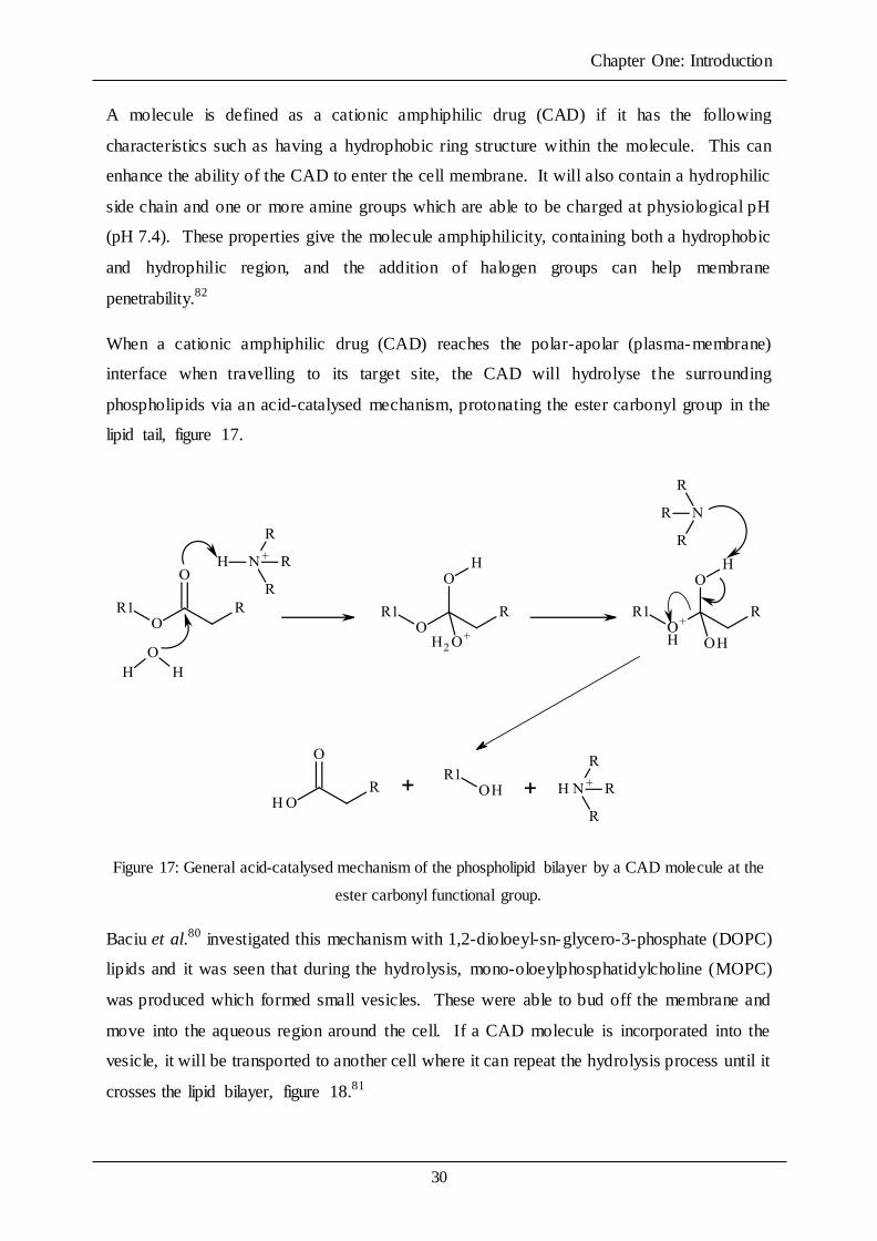
When a cationic amphiphilic drug (CAD) reaches the polar-apolar (plasma-membrane)
interface when travelling to its target site, the CAD will hydrolyse the surrounding
phospholipids via an acid-catalysed mechanism, protonating the ester carbonyl group in the
lipid tail, figure 17.
Figure 17: General acid-catalysed mechanism of the phospholipid bilayer by a CAD molecule at the
ester carbonyl functional group.
Baciu et al.80 investigated this mechanism with 1,2-dioloeyl-sn-glycero-3-phosphate (DOPC)
lipids and it was seen that during the hydrolysis, mono-oloeylphosphatidylcholine (MOPC)
was produced which formed small vesicles. These were able to bud off the membrane and
move into the aqueous region around the cell. If a CAD molecule is incorporated into the
vesicle, it will be transported to another cell where it can repeat the hydrolysis process until it
crosses the lipid bilayer, figure 18.81

Chapter One: Introduction
31
Figure 18: a) The CAD approaches the lipid bilayer; b) CAD molecules enter the bilayer due to
hydrophobic interactions; c) the CAD begins to hydrolyse the surrounding phospholipids; d) MOPC
begins to form vesicles around the CAD; e) Micelles bud off containing the MOPC and CAD which is
transported to neighbouring bilayers, taken from Casey et al.81
At the membrane-water interface, drug molecules, particularly CAD molecules, will rapidly
catalyse the hydrolysis mechanism which can depend on the properties of the drug molecule
itself.80 The rate of hydrolysis has previously been measured using artificial lipid models. It
was shown using fluorescence imaging studies that a CAD molecule will bind to a giant
unilamellar vesicle within milliseconds and begin the hydrolysis of the lipid bilayer as soon
as the drug has bound. Fluorescent images recorded indicated that hydrolysis of the ester
carbonyl bond occurred within 35 minutes showing degradation of the vesicle occurring on
time scales consistent with biological pharmacokinetics. Other experimental methods such as
NMR, small angle x-ray scattering and HPLC have shown that the rate of hydrolysis can take
several days to weeks, however the fluorescent studies are most likely to give the closest
approximation of the hydrolysis of a lipid bilayer in vivo.83
The acid dissociation constant, pKa, will have an effect on the rate of the hydrolysis of the
lipid membrane however as far as this author is aware, this has not been investigated and
quantified with respect to the affect pKa will have on the rate of lipid degradation and in turn
the affect this hydrolysis rate will have on the non-specific binding behaviour of a
radioligand.
Non-specific binding is a poorly understood phenomenon however the development of a
novel PET radioligand can be determined by this binding parameter. If NSB is too high, the
signal-to-background ratio will be too low and the radioligand will not be suitable for use as a
radiotracer and further development will be terminated. It is well established that increasing
lipophilicity will increase non-specific binding and within the literature, lipophilicity is the

Chapter One: Introduction
32
gold standard parameter used to predict possible non-specific binding behaviour. However it
has been shown that other physiochemical properties such as interaction energy may be
superior parameters for predicting the NSB of new radioligands.
It is clear that NSB is poorly understood and until the mechanisms that drive NSB are
investigated and clearly understood, potentially good PET radioligands will be discounted
during the development process due to poor predictions of its NSB behaviour.
1.6 Structure-Activity Relationships, SARs
In the pharmaceutical industry, the determination of new ligands for potential target receptor
sites can be obtained from large compound libraries. It is important for new lead compounds
that a provision of reliable predictions of the possible pharmacokinetic properties are
determined early in order to decide whether the lead compound will be suitable for further
development as a potential new drug.84
The initial development and optimisation of a new drug for a target receptor site can benefit
greatly from structure-activity relationships that have previously been formed for compounds
with similar structures. A structure-activity relationship (SAR) is a model relating the
chemical structure of a compound to its biological activity, property or effect it induces.85
The structure of a compound will implicitly determine its physical and chemical properties
which will determine its interactions in a biological system.
A series of compounds is usually designed and synthesised based on a compound with known
affinity for a particular target receptor. Quantifying the physical and chemical properties of
each derivative and relating this to the individual biological activity can give an indication as
to the best chemical structures to use and develop as potential new drugs.
SARs are predictive models and can show how similar molecules can have a dramatic change
in the activity or affinity with only a slight variation in the structure. The pharmaceutical
industry relies heavily on SARs in determining potential drug molecules to synthesise for
particular target sites and known SARs are usually applied as screening tools for choosing
new lead compounds.86
In the literature, a compound with a known affinity to a receptor is usually structurally
adapted to improve its affinity, selectivity or reduce its non-specific binding component.
Mokrosz et al.87 took a set of 1-arylpiperazine compounds which are known to have affinity

Chapter One: Introduction
33
for the 5-HT1A receptors in the human brain and formed a set of SARs to investigate how
various properties affect the affinity. It was seen that by changing various functional groups
the ionisation constants and connectivity indices could be varied. Relating these properties to
each affinity, Ki, measured it was shown that the binding site needed to be able to
accommodate a 6 – 8 carbon chain in order to be active.
Similarly Butini et al.88 showed that by changing the functionalisation in pyrroloquinoxaline
(PQX) derivatives, the affinity of each compound could be changed. The PQX was
functionalised with fluorine (F), methyl (Me) and hydroxyl (OH) groups and it was seen that
the affinity was highest for the fluorine derivative, followed by a methyl derivative and
finally the hydroxyl derivative. It was also shown that the addition of imidazol-5-ylmethyl
derivatives in the structure were the most potent compounds. From these various SARs, the
compound with the highest affinity can be developed further while the remaining data can be
used as a predictive tool for other compound series’.
Non-specific binding is a poorly understood phenomenon and little is known on the
mechanism of NSB however it is one of the major factors in the failure of radioligands in
PET imaging. The formation of structure-activity relationships relating physiochemical
properties of a series of compounds with their measured non-specific binding values is vital
to understanding NSB and producing predictive tools to aid PET radioligand development.
The predictive nature of the SARs that can be formed could lead to a better understanding of
NSB and improved predictive tools for determining potentially good radioligands reducing
time and cost of drug development.

Chapter One: Introduction
34
1.7 Structure-Activity Relationship (SAR) hypotheses
In this thesis, the structure-activity relationship between particular physicochemical
properties and non-specific binding are determined and the correlations observed have been
discussed. It is important before quantifying the SARs, that hypothesises are made to predict
the possible relationships that will arise. The hypotheses derived in this work are as follows:
Increasing the partition coefficient, lipophilicity, usually measured between an
aqueous and organic phase (water/n-octanol) will increase the amount of non-specific
binding observed in a PET image. This is because increasing the lipophilicity of a
molecule will lead to the compound remaining in the lipid bilayer rather than reaching
the target site under investigation.
Increasing the overall acid dissociation constant, pKa, of a molecule will decrease the
rate of hydrolysis as the compound will be a weaker acid and therefore it will
hydrolyse the lipid bilayer at a slower rate. This will lead to an increase in non-
specific binding at higher pKa values.
It is predicted that as the interaction energy of a lipid-drug complex decreases
(becomes more positive) the relative non-specific binding will decrease. This is
because the compounds will interact with the lipids less strongly. Instead the lower
interaction energy (more negative) will lead to stronger interactions with the lipid
bilayer and the drug molecule will enter the bilayer and remain there rather than
diffusing to its target site.
Increasing the molecular weight of a compound will make it harder to enter the lipid
bilayer as it will be too large to fit between the phospholipids and into gaps within the
lipid bilayer. This will in turn increase the overall non-specific binding observed in
the PET image.

Chapter One: Introduction
35
1.8 Aims and objectives
The aim of this work is to determine structure-activity relationships between novel positron
emission tomography radiotracers and their non-specific binding properties. Generally it is
considered that when a radiotracer has a low lipophilicity it will have a low non-specific
binding in vivo. However there are many exceptions to this rule, suggesting that other
physiochemical parameters need to be considered when designing novel radiotracers for PET
imaging. The parameters to be investigated in this work include the partition coefficient, acid
dissociation constant, interaction energy and molecular weight.
The aims of this work include;
Designing and synthesising a novel set of compounds with the ability to be
radiolabelled using carbon-11 isotopes. The compound series to be designed and
synthesised should be broad with varying physiochemical properties with no
particular target binding site in mind. This should lead to compounds having only
non-specific binding when measured in vitro;
Quantification of the physicochemical properties under investigation for each
compound using various experimental and computational techniques;
Use of known radiosynthesis techniques and experimental methods to radiolabel each
compound synthesised. Ideally [11C]CH3I should be used to alkylate each compound
via a O–, N– or S– alkylation;
Use of autoradiography techniques and the radiolabelled compounds synthesised to
measure the non-specific binding in vitro in rat brain tissue. After measuring the non-
specific binding properties of each radioligand, the NSB values should be compared
to each of the physiochemical properties to form structure-activity relationships
between each property and non-specific binding. From the SARs, a set of rules for
predicting the non-specific binding properties of the radioligand should be
determined;
Development of a non-radioactive assay for measuring non-specific binding
properties of compounds. This would help to understand the NSB of a compound in
the early stages of drug development without the need to use expensive radiolabelling
techniques. Ideally this new assay would be high-throughput allowing several
compounds to be measured in parallel.

Chapter One: Introduction
36
1.9 References
1. G. J. Tortora and S. R. Grabowski, Principles of Anatomy and Physiology, Ninth edn.,
John Wiley and Sons, New York, 2000.
2. Nature,
http://www.nature.com/horizon/livingfrontier/background/images/membrane_f2.jpg,
Accessed 12 November 2011.
3. S. R. Goodman, Medical Cell Biology, Lippincott-Raven, Philadelphia, 1998.
4. A. M. Seddon, D. Casey, R. V. Law, A. D. Gee, R. H. Templer and O. Ces, Chem.
Soc. Rev., 2009, 38, 2509-2519.
5. J. Cooper, The Biochemical Basis of Neuropharmacology, 8th edn., Oxford
University Press, New York, 2003.
6. L. A. A. de Jong, D. R. A. Uges, J. P. Franke and R. Bischoff, J. Chromatog. B.,
2005, 829, 1-25.
7. P. G. Strange, Biochem. J., 1988, 249, 309-318.
8. S. R. Cherry and M. Dahlbom, in PET: Molecular Imaging and Its Biological
Applications, ed. M. E. Phelps, Springer, New York, Editon edn., 2004, pp. 1-124.
9. M. Phelps, P. Natl. Acad. Sci., 2000, 97, 9226-9233.
10. A. D. Gee, Brit. Med. Bull., 2003, 65, 169-177.
11. H. R. Crane and C. C. Lauritsen, Int. Phys. Rev., 1934, 45, 497-498.
12. N. Satyamurthy, in PET: Molecular Imaging and Its Biological Applications, ed. M.
E. Phelps, Springer, New York, Editon edn., 2004, pp. 217-269.
13. A. D. Gee, American Pharm. Rev., 2006, 9, 39.
14. Z. Li and P. S. Conti, Adv. Drug. Deliver. Rev., 2010, 62, 1031-1951.
15. P. W. Miller, N. J. Long, R. Vilar and A. D. Gee, Angew. Chem. Int. Edit., 2008, 47,
8998-9033.
16. H. Audrain, Angew. Chem. Int. Edit., 2007, 46, 1772-1775.
17. P. H. Elsinga, Methods, 2002, 27, 208-217.
18. M. Allard, E. Fouquet, D. James and M. Szlosek-Pinaud, Curr. Med. Chem., 2008,
15, 235-277.
19. D. J. Schlyer, Annal. Acad. Med., 2004, 33, 146-154.
20. B. Långström, O. Itsenko and O. Rahman, J. Labelled. Compd. Rad., 2007, 50, 794-
810.
21. B. Långström and H. Lunsqvist, Int. J. Appl. Radiat. Is., 1976, 27, 357-363.

Chapter One: Introduction
37
22. M. Bergström, A. Grahnén and B. Långström, Eur. J.Clin. Pharmacol., 2003, 59,
357-366.
23. Z. Tu and R. H. Mach, Curr. Top. Med. Chem., 2010, 10, 1060-1095.
24. S. L. Pimlott and A. Sutherland, Chem. Soc. Rev., 2010.
25. D. C. Costa, Radiat. Phys. Chem., 2007, 76, 357-359.
26. B. Andrée, C. Halldin, V. W. Pike, R. Gunn, H. Olsson and L. Farde, J. Nucl. Med.,
2002, 43, 292-303.
27. H. Hall, C. Lundkvist, C. Halldin, L. Farde, V. W. Pike, J. A. McCarron, A. Fletcher,
I. A. Cliffe, T. Barf, H. Wikström and G. Sedvall, Brain. Res., 1997, 745, 96-108.
28. J.-C. Martel, N. Leduc, A.-M. Ormiere, V. Faucillon, N. Danty, C. Culie, D. Cussac
and A. Newman-Tancredi, Eur. J. Pharmacol., 2007, 574, 15-19.
29. D. Le Bars, J. Fluorine Chem., 2006, 127, 1488-1493.
30. B. J. Fueger, K. Yeom, J. Czernin, J. W. Sayre, M. E. Phelps and M. S. Allen-
Auerbach, Mol. Imaging. Biol., 2009.
31. G. Lappin and R. C. Garner, Nat. Rev. Drug Discov., 2003, 2, 233-240.
32. J. A. DiMasi, Clin. Pharmacol. Ther., 2001, 69, 297-307.
33. C.-M. Lee and L. Farde, Trends. Pharmacol. Sci., 2006, 27, 310-316.
34. K. Serdons, A. Verbruggen and G. M. Bormans, Methods, 2009, 48, 104-111.
35. V. J. Cunningham, C. A. Parker, E. A. Rabiner, A. D. Gee and R. N. Gunn, Drug.
Discov. Today., 2005, 2, 311-315.
36. S. J. Gately and F. I. Carroll, Drug. Develop. Res., 2003, 59, 191-193.
37. I. M. Klotz, Q. Rev. Biophys., 1985, 18, 227-259.
38. M. Slifstein and M. Laruelle, Nucl. Med. Biol., 2001, 28, 595-608.
39. W. C. Eckelman, Nucl. Med. Biol., 1989, 16, 233-245.
40. W. C. Eckelman, R. C. Reba, R. E. Gibson, W. J. Rzeszotarski, F. Vieras, J. K.
Mazaitis and B. Francis, J. Nucl. Med., 1979, 20, 350-357.
41. R. B. Innis, V. J. Cunningham, J. Delforge, M. Fujita, A. Gjedde, R. N. Gunn, J.
Holden, S. Houle, S.-C. Huang, M. Ichise, H. Iida, H. Ito, Y. Kimura, R. A. Koeppe,
G. M. Knudsen, J. Knuuti, A. A. Lammertsma, M. Laruelle, J. Logan, R. P. Maguire,
M. A. Mintun, E. D. Morris, R. Parsey, J. C. Price, M. Slifstein, V. Sossi, T. Suhara,
J. R. Votaw, D. F. Wong and R. E. Carson, J. Cereb. Blood Flow Metab., 2007, 27,
1533-1539.
42. M. A. Mintun, M. E. Raichle, M. R. Kilbourn, G. F. Wooten and M. J. Welch, Ann.
Neurol., 1984, 15, 217-227.

Chapter One: Introduction
38
43. J. Logan, J. S. Fowler, N. D. Volkow, A. P. Wolf, S. L. Dewey, D. J. Schlyer, R. R.
MacGregor, R. Hitzemann, B. Bendriem, S. J. Gatley and D. R. Christman, J. Cereb.
Blood. Flow. Metab., 1990, 10, 740-747.
44. J. Logan, Nucl. Med. Biol., 2000, 27, 661-670.
45. A. A. Lammertsma and S. P. Hume, Neuroimage, 1996, 4, 153-158.
46. R. A. Koeppe, V. A. Holthoff, K. A. Frey, M. R. Kilbourn and D. E. Kuhl, J. Cereb.
Blood. Flow. Metab., 1991, 11, 735-744.
47. M. Laruelle, Eur. J. Nucl. Med., 1999, 26, 571-572.
48. H. M. Bigott-Hennkens, S. Dannoon, M. R. Lewis and S. S. Jurisson, Q. J. Nucl.
Med., 2008, 52, 245-253.
49. A. P. Davenport and F. D. Russell, in Current Directions in Radiopharmaceutical
Research and Development, ed. S. J. Mather, Kluwer Academic Publishers,
Netherlands, Editon edn., 1996, pp. 169-179.
50. G. Scatchard, Annals New York Academy of Sciences, 1949, 660-672.
51. M. D. Hall and V. W. Pike, J. Nucl. Med., 2011, 52, 338-340.
52. J. Passchier, A. D. Gee, A. Willemsen, W. Vaalburg and A. van Waarde, Methods,
2002, 27, 278-286.
53. W. M. Pardridge, Adv. Drug. Deliver. Rev., 1995, 15, 5-36.
54. W. M. Pardridge, J. Neurochem., 1998, 70, 1781-1792.
55. C. A. Lipinski, F. Lombardo, B. W. Dominy and P. J. Feeney, Adv. Drug. Deliver.
Rev., 1997, 23, 3-25.
56. C. M. Mendel and D. B. Mendel, Biochem. J., 1985, 228, 269-272.
57. L. Rosso, A. D. Gee and I. R. Gould, J. Comput. Chem., 2008, 29, 2397-2405.
58. C. Halldin, B. Gulyás, O. Langer and L. Farde, Q. J. Nucl. Med., 2001, 45, 139-152.
59. F. Kügler, W. Sihver, J. Ermert, H. Hübner, P. Gmeiner, O. Prante and H. H. Coenen,
J. Med. Chem., ASAP.
60. W. C. Eckelman, M. R. Kilbourn and C. A. Mathis, Nucl. Med. Biol., 2009, 36.
61. R. N. Gunn, S. R. Gunn, F. E. Turkheimer, J. A. D. Aston and V. J. Cunningham, J.
Cereb. Blood. Flow. Metab., 2002, 22, 1425-1439.
62. R. N. Waterhouse, Mol. Imaging. Biol., 2003, 5, 376-389.
63. S. Sebai, M. Baciu, O. Ces, J. Clarke, V. Cunningham, R. Gunn, R. Law, X. Mulet, C.
Parker, C. Plisson, R. Templer and A. Gee, Neuroimage, 2006, 31, Supplement 2,
T56.
64. M. Kah and C. D. Brown, Chemosphere, 2008, 72, 1401-1408.

Chapter One: Introduction
39
65. B. Sethi, M. Soni, S. Kumar, G. D. Gupta, S. Mishra and R. Singh, J. Pharm. Res.,
2010, 3, 345-351.
66. K. Valko, J. Chromatog. A., 2004, 1037, 299-310.
67. K. Valko, C. M. Du, C. Bevan, D. P. Reynolds and M. H. Abraham, Curr. Med.
Chem., 2001, 8, 1137-1146.
68. N. A. Kratochwil, W. Huber, F. Muller, M. Kansy and P. R. Gerber, Biochem.
Pharmacol., 2002, 64, 1355-1374.
69. D. D. Dishino, M. J. Welch, M. R. Kilbourn and M. E. Radichle, J. Nucl. Med., 1983,
24, 1030.
70. S. Marchais, B. Nowicki, H. Wikström, L. T. Brennum, C. Halldin and V. W. Pike,
Bioorgan. Med. Chem., 2001, 9, 695-702.
71. H. Ito, C. Halldin and L. Farde, J. Nucl. Med., 1999, 40, 102-109.
72. Z. Jiang, J. Reilly, B. Everatt and E. Briard, J. Pharmaceut. Biomed., 2011, 54, 722-
729.
73. A. A. Wilson, A. Garcia, A. Chestakova and S. Houle, Neuroimage, 2004, 22, T61-
T200.
74. C. Pidgeon, S. Ong, H. Liu, X. Qiu, M. Pidgeon, A. H. Dantzig, J. Munroe, W. J.
Hornback, J. S. Kasher, L. Glunz and T. Szczerba, J. Med. Chem., 1995, 38, 590-594.
75. C. Giaginis and A. Tsantili-Kakoulidou, J. Pharm. Sci., 2008, 97, 2984-3004.
76. C. J. Dickson, A. D. Gee, I. Bennacef, I. R. Gould and L. Rosso, Phys. Chem. Chem.
Phys., 2011, ASAP.
77. X. Kong, T. Zhou, Z. Liu and R. C. Hider, J. Pharm. Sci., 2007, 96, 2777-2783.
78. M. Remko, M. Swart and F. M. Bickelhaupt, Bioorgan. Med. Chem., 2006, 14, 1715-
1728.
79. G. Roda, C. Dallanoce, G. Grazioso, V. Liberti and M. De Amici, Anal. Sci., 2010,
26, 51-54.
80. M. Baciu, S. C. Sebai, O. Ces, X. Mulet, J. A. Clarke, G. C. Shearman, R. V. Law, R.
H. Templer, C. Plisson, C. A. Parker and A. D. Gee, Philos. T. Roy. Soc. A, 2006,
364, 2597.
81. D. R. Casey, S. C. Sebai, G. C. Shearman, O. Ces, R. V. Law, R. H. Templer and A.
D. Gee, Ind. Eng. Chem. Res., 2008, 47, 650.
82. W. H. Halliwell, Toxicol. Pathol., 1997, 25, 53-60.
83. S. C. Sebai, PhD. Thesis, Imperial College London, 2007.

Chapter One: Introduction
40
84. S. G. Summerfield, A. J. Lucas, R. A. Porter, P. Jeffrey, R. Gunn, K. R. Read, A. J.
Stevens, A. C. Metcalf, M. C. Osuna, P. J. Kilford, J. Passchier and A. D. Ruffo,
Xenobiotica, 2008, 38, 1518-1535.
85. J. D. McKinney, A. Richard, C. Waller, M. C. Newman and F. Gerberick, Editon
edn., 2000, vol. 56, pp. 8-17.
86. R. Kunal, Expert Opin. Drug Discov., 2007, 2, 1567-1577.
87. J. L. Mokrosz, M. Pietrasiewicz, B. Duszynska and M. T. Cegla, J. Med. Chem.,
1992, 35, 2369-2374.
88. S. Butini, R. Budriesi, E. Hamon, S. Gemma, M. Brindisi, G. Borrelli, E. Novellino, I.
Fiorini, P. Ioan, A. Chiarini, A. Cagnotto, T. Mennini, C. Fracasso, S. Caccia and G.
Campiani, J. Med. Chem., 2009, 52, 6946-6950.

CHAPTER TWO:
ORGANIC SYNTHESIS

Chapter Two: Organic Synthesis
42
2.0 CHAPTER TWO: ORGANIC SYNTHESIS
2.1 Introduction
It is generally assumed that lipophilicity is one of the factors influencing NSB. There are
however several exceptions to this rule of thumb which suggests that other physiochemical
parameters have an impact on non-specific binding. For example WAY 100635, refer to
figure 8 in chapter one,1 has very low NSB in vivo, but is considered to be reasonably
lipophilic.
2.1.1 Designing compound libraries
It can sometimes be useful in the pharmaceutical industry to design a compound library,
synthesised through combinatorial synthesis, containing a series of ligands that can be
investigated for SARs to a particular target. It is usually best to design a targeted library of
compounds containing various derivatives of a known structure. This can be achieved by
selecting a backbone structure and varying the synthon added. A synthon is a functional
group added at a particular point in the synthesis, usually a molecular fragment rather than a
reagent. A common feature of the compound library is the ability to use the same chemical
reactions to synthesise each compound while substituting one reagent to vary the final
compound.2
In this work a small library containing nine compounds, to be radiolabelled, has been
synthesised in order to vary the physiochemical properties and investigate how each property
will affect the non-specific binding observed for each PET ligand. The compound library
designed aimed to have a broad range of physiochemical properties and was designed not to
bind to a specific target protein.
2.1.2 Designing compounds for investigating non-specific binding
The 1-(hydroxyphenyl)-piperazine group was taken as the common moiety in all compounds
allowing the addition of various functional groups on the piperazine ring to change the
physicochemical properties accordingly. This moiety also contains a hydroxyl, -OH, group
which can be used as the position to radiolabel using known labelling methods as discussed
in chapter 5.
The main properties under investigation are the lipophilicity of a compound, its affinity for a
lipophilic environment such as oil, fats and lipids3, and the acid dissociation constant, pKa.

Chapter Two: Organic Synthesis
43
In order to increase the lipophilicity of each molecule while keeping other parameters as
constant as possible, alkyl chains of various lengths were added. It is predicted that longer
alkyl chains will increase the lipophilicity increasing the molecules’ affinity for an oil, fat or
lipid environment.
The acid dissociation constant, pKa, of a molecule is assumed to be important as it is
suggested that 60-70 % of drugs are ionisable molecules and many biological processes are
dependent on this parameter.4 In this work the pKa was varied in the molecules by the
addition of benzyl, pyridyl and carboxylate ester functional groups. A discussion of the
physicochemical properties and quantification of each parameter is discussed in chapter 3.
2.1.3 The piperazine functional group
The piperazine functional group was chosen as the backbone to all the compounds in this
series as it is a widely used moiety in many drug-like molecules, such as WAY 100635.5, 6
It
also provides a position for radiolabelling and a position to attach various functional groups
at the piperazine –NH group. This moiety has also been seen to be important for receptor
affinity and specificity, and to possess biological activity by having specific interactions with
G-protein-coupled receptors.7
The 1-(2-methoxyphenyl)piperazine moiety was chosen as the main functional group within
each molecule to provide a position to radiolabel with [11
C]methyl iodide. This compound
also has the advantage that the amine group, R2NH, present in the piperazine ring is readily
available to react with various aldehyde compounds in condensation reactions.
It was decided that to increase the lipophilicity of each compound an alkyl chain with an
increasing number of carbon atoms present would be covalently bonded to the amine group.
This would increase the lipophilicity of each molecule, without varying other physiochemical
properties to too large an extent. Instead of the alkyl chain attached to the piperazine group,
benzyl, pyridyl and carboxylate ester groups were used to vary the pKa values and interaction
energy of each compound.

Chapter Two: Organic Synthesis
44
The compounds in this work were not designed to target a specific receptor however it has
been seen in the literature that a high number of drugs containing the 1-(2-
methoxyphenyl)piperazine moiety have an affinity for serotonin receptors, 5HT, found in the
brain. They have also been seen to target adrenergic and dopaminergic receptors.4
Serotonin is an important family of receptors and plays a role in anxiety and depression. It
has been suggested that 5HT1A receptor agonists have neuroprotective properties, while the
antagonist could play a vital role in the treatment of many cognitive diseases.8 With an ever
increasing interest and understanding as to the vital role serotonin plays in the human body,
an increasing number of research groups have begun investigating various structure-activity
relationships with piperazine-based ligands.9-11
2.2 Results and Discussion
Both the hydroxyphenyl, figure 1, and the methoxyphenyl, figure 2, derivatives were
synthesised.
Figure 1: 1-(2-Hydroxyphenyl)piperazine derivatives synthesised compounds 1 to 9

Chapter Two: Organic Synthesis
45
Figure 2: 1-(2-Methoxyphenyl)piperazine derivatives synthesised compounds 10 – 18
All compounds synthesised in this work have been previously reported within the literature
and were synthesised using known synthetic methods. Compounds 1 to 9 are hydroxyphenyl
precursors to be used in the radiosynthesis reactions. Compound 10 to 18 were synthesised to
quantify each physiochemical parameter under investigation and to use as reference
compounds to determine product formation during radiosynthesis.
2.2.1 Synthesis of 1-(2-hydroxyphenyl)piperazine derivatives, compounds 1 – 9
Compound 1, 1-(2-hydroxyphenyl)piperazine, was purchased from Sigma Aldrich and used
as supplied. This compound was used in the synthesis of compounds 2 to 9, as well as
making up part of the series of compounds under investigation.
Lacivita et al. suggested a simple, rapid, one-pot synthesis method for the production of all
compounds 1 – 9.4 In this reaction 1-(2-hydroxyphenyl)piperazine was dissolved in methanol
and the corresponding alkyl aldehyde was added slowly at room temperature. This was left
to stir under nitrogen for an hour before the intermediate enamine was reduced by the slow
addition of sodium borohydride at 0oC. The reaction was left to stir for two hours at room
temperature before the solution was quenched with water. The crude product was formed
with no side products and purification was needed to remove unreacted starting material.

Chapter Two: Organic Synthesis
46
Figure 3: One pot synthesis of compounds 1 – 9
Purification of each compound was carried out on a Teledyne Isco Combiflash purification
system at CIC GSK, Hammersmith Hospital. Neutral alumina pre-packed cartridges with a
gradient solvent system of ethyl acetate and hexane were used providing a rapid purification
system. All compound purifications followed the same method with ethyl acetate started at
0% before being increased to 100% over 15 column lengths. Hydroxyphenyl derivatives,
compounds 1 to 6, formed white crystalline solids.
This reaction worked well for the synthesis of each compound in this series leading to a
simple, rapid one pot synthesis reaction. The ability to synthesise, work-up and purify each
compound in a single day made this a reliable high-throughput method.
The alkylation of the piperazine group occurs rapidly and involves the lone pair on the
nitrogen group attacking the carbonyl carbon in the aldehyde reagent. After hydrogen
rearrangement, the nitrogen lone pair is able to attack the alcohol carbon forcing the removal
of the alcohol group and forming a double bond enamine structure. The addition of sodium
borohydride inserts a hydrogen atom across the double bond reducing the intermediate to the
product, figure 4.

Chapter Two: Organic Synthesis
47
Figure 4: Reaction mechanism for the synthesis of 1-(2-hydroxyphenyl)-4-propylpiperazine, 3, and
reduction to the final product
When attempting to synthesise compounds 7 – 9 it was seen that it was not possible to carry
out the same condensation using the relevant aldehyde reagents. Instead these compounds
were synthesised using chloride derivatives and triethylamine dissolved in acetonitrile.
Reaction solutions were left stirring over 2 days at room temperature and purification was
carried out on alumina neutral gravity columns using either a composition of hexane:ethyl
acetate or dichloromethane:methanol as the mobile phase, figure 5.

Chapter Two: Organic Synthesis
48
Figure 5: Synthesis of 1-(2-hydroxyphenyl)piperazine derivatives 7 – 9
The synthesis of each compound produced low yields. The products however were obtained
with a good purity and have been fully characterised.
Each 1H NMR spectrum recorded contains 4 peaks in the aromatic region representing the
phenyl protons attached to the piperazine ring. Coupling constants and chemical shifts are as
expected and indicate the presence of a functional group attached at position-2 in the
aromatic ring, (figure 6). All proton environments are accounted for within the 1H NMR
data except for the hydroxyl functional groups. Hydroxyl groups are regularly seen in 1H
NMR spectra as very broad small peaks at around 5 ppm or are not observed at all. This is
due to proton exchange occurring between the proton in the hydroxyl group and atoms in the
deuterated solvent. This exchange is rapid and causes broadening of a peak and can render it
invisible. This process is also often seen in amine functional groups.

Chapter Two: Organic Synthesis
49
Figure 6: 1H NMR spectra of hydroxyphenyl derivatives, compound 1 to 6 in deuterated chloroform
Figure 7: 1H NMR spectra of the alkyl carbon chain chemical shifts in deuterated chloroform,
showing the increasing number of peaks as the chain length increases

Chapter Two: Organic Synthesis
50
From the 1H NMR spectra, figure 7, it can be seen that addition of the alkyl chain on the
piperazine ring causes the proton peak at 2.85 ppm to change from a triplet peak to a broad
singlet at the same chemical shift. This is explained in detail in section 2.3.3. As the alkyl
chain length increases the individual proton environments in the longer chain lengths are seen
to have similar chemical shifts forcing the peaks to overlap and appear as multiplets at
approximately 1.35 ppm. This is also seen in the 1H NMR spectra of compounds 7 to 9,
containing a benzyl (7), pyridyl (8) and carboxylate ester (9) groups. The aromatic region in
the NMR spectra for compounds 7 and 8 contains several more proton peaks and no peaks are
observed in the aliphatic region as expected. In the 1H NMR spectrum of compound 9 the
presence of a singlet peak for the carboxylate ester protons at 3.8 ppm indicates the formation
of this compound.
Infrared spectroscopy indicates that the hydroxyl group is present in each compound as
expected with a broad small peak at approximately 3340 cm-1
. This is the main feature of the
IR spectra and confirms the presence of the –OH group needed for radiolabelling each
compound. This was important as 1H NMR was not necessarily able to distinguish the
hydroxyl proton due to rapid proton exchange.
Mass spectrometry showed that compounds 2 to 9 were synthesised with their molecular ions
giving a 100% peak at the expected m/z. Characterisation data of compounds previously
synthesised in the literature correlates well with data recorded.
2.2.2 Synthesis of 1-(2-methoxyphenyl)piperazine derivatives, compounds 10 - 18
Compound 10, 1-(2-methoxyphenyl)piperazine, was purchased from Sigma Aldrich and used
as supplied. This compound was used in the synthesis of compounds 11 to 18, as well as
making up part of the series of compounds under investigation.
The synthesis of 1-(2-methoxyphenyl)piperazine derivatives, compounds 10 to 18, was rapid
and high-throughput producing compounds of high purity in average yields. It was necessary
to synthesise the methylated derivatives as these are used as reference samples for
confirmation for the production of the desired radiotracer during radiosynthesis reactions.

Chapter Two: Organic Synthesis
51
The same synthesis was adopted for this group of compounds using 1-(2-
methoxyphenyl)piperazine as the starting reagent and the relevant aldehyde with stirring at
room temperature for an hour before sodium borohydride was added to reduce the enamine
bond present in the intermediate.
Figure 8: One pot synthesis of 1-(2-methoxyphenyl)piperazine derivatives, compounds 10 – 15
The same purification system was used and the same reaction mechanism has been proposed
for this set of compounds as was seen for the hydroxyphenyl derivatives. Pale yellow oils
were isolated for most compounds except compound 15 which formed as a clear oil.
Compounds 16 – 18 were not able to be synthesised using the same reaction conditions as
compounds 10 – 15. As such, these compounds were synthesised using chloride derivatives
and triethylamine dissolved in acetonitrile. Each solution was left stirring over 2 days at
room temperature and purification was carried out on alumina neutral gravity columns using
either a composition of hexane:ethyl acetate or dichloromethane:methanol as the mobile
phase, figure 9.
Figure 9: Synthesis of 1-(2-hydroxyphenyl)piperazine derivatives 16 – 18

Chapter Two: Organic Synthesis
52
Each of these compounds were successfully synthesised however low yields were obtained.
Products were obtained with a high purity and have been fully characterised (see
experimental section).
The characterisation data of the methoxyphenyl derivatives, compounds 10 – 18 was seen to
have many similarities when compared to the spectral data collected for the hydroxyphenyl
derivatives. Due to the similarity of the compound structures, it is important to characterise
each compound using multiple techniques. Elemental analysis and mass spectrometry were
collected for each compound and used to determine the mass and the purity of the final
methoxyphenyl compounds synthesised. Infra-red spectra were also used to show the lack of
the hydroxyl group in these compounds.
The 1
H NMR spectrum recorded for each 1-(2-methoxyphenyl)piperazine derivative contains
the characteristic signals in the aromatic region between 6.5 and 7.0 ppm. The aromatic
region appears at a similar chemical shift as seen in the 1H NMR spectra for the
hydroxyphenyl derivatives however due to the addition of the –CH3 group on the oxygen
atom, overlapping of the proton peaks is observed and the region appears as a complicated
multiplet rather than separate doublet and triplet peaks, figure 10. This is due to the protons
in the –OCH3 group coupling to the aromatic ring protons through space.
Figure 10: 1H NMR spectrum of 1-(2-methoxyphenyl)-4-butylpiperazine and an enlarged image of the
aromatic region

Chapter Two: Organic Synthesis
53
Another characteristic peak observed in all the methylated derivatives is the presence of a
peak at approximately 3.8 ppm. This peak has an integration of three and represents the
protons present in the –OCH3 group which is the main difference between the hydroxyphenyl
and methoxyphenyl compounds’ 1H NMR data. As the alkyl chain is increased the addition
of new peaks between 1.0 and 2.5 ppm is observed as seen in the 1H NMR spectra of the
hydroxyphenyl compounds.
Infrared spectroscopy was used to indicate the loss of a broad peak at approximately 3340
cm-1
indicating the lack of a hydroxyl group in the aromatic ring. The IR spectrum for each
methyoxyphenyl derivative 10 to 18 all appear to be similar and have characteristic stretches
and bending peaks in the spectra. The most important peak is seen at approximately 1280
cm-1
in all six spectra recorded. This indicates the presence of the –O-C stretching bond in
the –OCH3 group and is not present in the spectra recorded for the hydroxyphenyl
compounds.
2.2.3 1H NMR spectra characteristic peaks
a) Changes between the hydroxyphenyl and methoxyphenyl compounds
in the aromatic proton region
The 1H NMR spectra recorded for the hydroxyphenyl and methoxyphenyl compounds vary
dramatically in the aromatic region, 7.2 – 6.5 ppm. Compounds 1 to 9, hydroxyphenyl
derivatives, show single peaks for each of the protons present in the ring. The proton HA
neighbouring the methoxy group in the aromatic ring (figure 11) gives a double doublet due
to ortho-coupling to HB and a small amount of meta-coupling with Hc, 4JHAHC see at 7.2 ppm.
The second double doublet at 6.9 ppm is caused by a similar coupling pattern of HD to HC
(ortho-coupling), and to HB (meta-coupling). The peaks observed at 6.8 and 7.1 ppm
represent protons HB and HC respectively. Both protons will couple with each neighbouring
proton (3JHBHA,
3JHBHC) as well as meta-coupling with HD or HA (
4JHBHD and
4JHCHA) giving a
doublet of doublet of doublets (ddd).

Chapter Two: Organic Synthesis
54
Figure 11: Aromatic protons in 1-(2-hydroxyphenyl)-4-methyl-piperazine
In the 1H NMR spectra for compounds 10 to 18, the methoxyphenyl derivatives, it is
observed that proton peaks overlap and the individual proton environments are difficult to
define. Instead broadening and overlapping of the aromatic proton peaks is recorded (figure
12).
Figure 12: The change in the 1H NMR aromatic region (6 – 7 ppm) from the hydroxyphenyl
derivatives to the methoxyphenyl derivatives
It is unclear as to the reasoning to this broadening pattern observed in the 1H NMR. It was
suggested that through-space coupling between the aromatic protons and the piperazine or
methoxy protons could be causing this overlapping of peaks and as such a NOESY NMR was
preformed.
Through-space coupling can be observed using Nuclear Overhauser Effect Spectroscopy,
NOESY 1H NMR. NOESY NMR is a spectroscopic technique used to correlate protons in
close proximity to one another. When atoms are close enough, through-space coupling can
be observed. This is due to the nuclear overhauser effect, NOE, which is where there is a
transfer of nuclear spin polarisation from one atom spin to another through space.12
This type
of spectroscopy produces cross peaks in a 2D NMR spectrum and was recorded for
compound 13, figure 13.

Chapter Two: Organic Synthesis
55
Figure 13: 1H NOESY NMR spectrum of compound 13
The spectrum shows a diagonal signal (blue regions) which can be ignored as these indicate a
proton atom is coupling with itself. Protons coupling through-space with a close proximity
proton are indicated by red regions in the spectrum. From the 2D 1H NMR spectrum it can
be seen that there is a degree of through-space coupling between the piperazine protons and
aromatic protons seen by a red region at (f1, f2) 3.2, 6.9 ppm. However it is unlikely that this
interaction would cause all the peaks in the aromatic region to overlap and broaden. It was
initially thought that the addition of the methyl protons on the phenolic ring could affect the
chemical shifts by interacting with the aromatic protons or with the piperazine protons
however if this was the case, it would be expected to see a red region at (f1, f2) 3.8, 3.0 ppm.
The change in the aromatic region in the 1H NMR is unexpected and is not well documented
in the literature and the NOESY NMR has not led to a possible explanation.
b) Broadening of the piperazine proton peaks
Another similar pattern observed in the spectra is the broadening of the piperazine proton
peaks. In compounds 2 to 9, only one proton environment is seen to form a broad singlet at
approximately 3.0 ppm due to the addition of the alkyl chain, benzyl or pyridyl group.

Chapter Two: Organic Synthesis
56
However in compounds 10 to 18, broadening of both piperazine proton environments occurs,
figure 14.
Figure 14: 1H NMR spectrum of the piperazine proton region for methylated compounds 10 – 18
Firstly, for all compounds 2 – 18, the addition of an alkyl chain to the piperazine ring at N2
causes the aliphatic protons to appear as a broad singlet at approximately 2.50 ppm. The
appearance of a broad singlet is unexpected and has been documented in the literature for
similar compounds however an explanation for such a phenomenon has not been suggested.4
It can also be seen from the NOESY 1H NMR, figure 14, that the alkyl chain protons interact
with the piperazine protons causing the piperazine peaks to broaden and appear as singlets
rather than triplets. From the spectrum, protons on the second carbon in the alkyl chain
couple with the piperazine ring through-space. Usually the protons on this carbon are too far
away from the ring to induce any coupling, however, the alkyl chain could be bending back
on itself, coming closer to the piperazine ring and therefore allowing some through-space
coupling to occur.
Secondly, it is seen for compounds 10 – 18, protons adjacent to N1 in the piperazine ring are
broadened due to the addition of the methyl group on the aromatic ring.
It may be possible that before the piperazine ring is alkylated it is able to rapidly fluctuate
between conformers, figure 15.7 However on the addition of the alkyl chain at the N-2
position the fluctuations are slowed causing broadening in the NMR peaks. Before the alkyl
chain is incorporated into the compound the piperazine ring is able to flip at a faster rate than
the 1H NMR process is able to distinguish between each proton in the ring and the coupling

Chapter Two: Organic Synthesis
57
occurring within the molecule produces a triplet. On the addition of the alkyl group, the
nitrogen is unable to flip at the same rate and the 1H NMR records a chemical shift for both
conformers in solution which broadens the peak to a broad singlet.13
Figure 15: Ring fluctuating about the piperazine functional group
Temperature dependent 1H NMR experiments were used to investigate this theory and show
that as the temperature of the solution is increased, the piperazine ring has more energy and is
able to fluctuate more rapidly. The temperature dependent 1H NMR spectra was recorded for
1-(2-methoxyphenyl)-4-butyl-piperazine, compound 12, ranging from a temperature of 233 K
to 313 K, figure 16.
Figure 16: Temperature dependent 1H NMR spectra of the methoxyphenyl derivative compound 12,
ranging from 233K to 313K
The 1H NMR spectrum of 1-(2-methoxyphenyl)-4-butyl-piperazine, compound 12, was
recorded and a variation in the peaks over the temperature range can be seen, figure 16. At
room temperature, 293 K (dark blue line) the piperazine proton peaks appear as two broad
singlets. As the temperature is increased the molecule has more energy and is able to
fluctuate and bend at a faster rate. This fluctuation occurs at too fast a rate to decipher
between the individual conformers and the overall structure is averaged out. This causes the

Chapter Two: Organic Synthesis
58
broad singlets to appear as two triplets, one triplet representing protons Ha and Hb (figure 16),
and one representing the protons Hc and Hd.
As the temperature is lowered to 233 K in 10 K increments, the broad singlets first disappear
(263 K) before reappearing as two doublets at 3.45 and 3.00 ppm indicating the presence of
Ha and Hb, and a separate triplet at 2.75 ppm for Hc. It would be predicted, that if Ha and Hb
were in different environments the spectrum would appear as two doublets of triplets and a
double doublet. However, it could be possible that the protons have similar chemical shifts
leading to broad overlapping peaks. Integration of each peak shows that the correct number
of protons is represented in the spectrum.
Each doublet can be assigned to proton Ha and Hb respectively, while the triplet is caused by
Hc protons. As the temperature is reduced, the molecule rotates and vibrates at a slower rate
and the most energetically favourable conformer is detected by the NMR machine. Ha and
Hb appear to be in different environments due to the methoxy group present in the aromatic
ring. The oxygen atom hydrogen bonds with proton Ha on either side of the nitrogen in the
piperazine ring forcing it to have a different chemical shift to Hb. As the alkyl chain is unable
to hydrogen bond to the Hc protons in the ring, both protons appear to be in the same
environment forming a triplet in the 1H NMR spectrum.
The broadening of piperazine ring protons has been noted in the literature previously but little
has been done to explain the phenomenon.7 Temperature dependent
1H NMR spectra have
shown that by heating the sample, the molecule will have more energy and it is possible to
force the proton peaks to form triplet peaks as would be expected. It has also been shown
that the protons in the aromatic ring and alkyl chain couple to the piperazine protons through
space, broadening the peaks further.
Overall the addition of the methoxy group, -OMe, on the aromatic ring allows the protons in
the piperazine ring to interact with the methoxy protons via through-space coupling. This
causes the broadening of the proton peaks at 3.5 ppm. The alkyl chain at the N2 position
causes the piperazine ring to flip at the slower rate and the alkyl protons are able to interact
with the piperazine protons via through-space coupling. This causes broadening of the proton
peak at 2.5 ppm.

Chapter Two: Organic Synthesis
59
2.3 Experimental
2.3.1 General Instructions
All reagents were used as received from commercial suppliers. Compounds 1 and 10 were
used as received from Sigma Aldrich for all experiments and lipophilicity measurements.
Glassware was thoroughly cleaned and dried prior to use. 1H and
13C NMR spectra were
obtained at room temperature using Bruker 400 MHz spectrometers. Chemical shifts are
recorded relative to internal solvent standards. Infrared spectra were obtained using a Perkin
Elmer FT-IR Spectrometer Paragon 1000. Mass spectrometry (ESI) was carried out on a
Micromass LCT Premier instrument at Imperial College London, UK. Elemental analyses
were carried out on a Carlo Erba CE1108 Elemental Analyser at London Metropolitan
University, UK.
2.3.2 Synthesis of 1-(2-hydroxyphenyl)piperazine derivatives 2 - 6
All compounds synthesised in this work have been previously reported within the literature
and were synthesised using previously known methods by Lacivita et al.4 1-(2-
Hydroxyphenyl)piperazine derivatives 2 – 6 were synthesised following the same procedure13
with the corresponding aldehyde obtained from Sigma Aldrich and used as supplied.
To a solution of 1-(2-hydroxyphenyl)piperazine (535 mg, 3.0 mmol) in methanol (20 ml), the
appropriate aldehyde (3.6 mmol) was added dropwise and the solution stirred at room
temperature for 1 hour. After cooling to 0oC, sodium borohydride (170 mg, 4.5 mmol) was
added in small portions. The mixture was warmed to room temperature and left to stir for 2
hours and then quenched with water. Methanol was reduced under pressure and the aqueous
solution extracted with dichloromethane (3 x 20 ml). The organic phases were collected and
washed with brine solution and dried over Na2SO4 and concentrated in vacuo.
Samples were purified using a Teledyne Isco Combiflash using a gradient solvent system of
hexane and ethyl acetate and alumina neutral pre-packed columns. Ethyl acetate was initially
started at 0 % and over the period of 15 column lengths the percentage was increased to 100
%.

Chapter Two: Organic Synthesis
60
a) 1-(2-Hydroxyphenyl)-4-methylpiperazine (2)
A white crystalline solid (yield: 398 mg, 69 %, m.p: 75 – 79 oC):
1H NMR (400 MHz, CDCl3,
ppm): δ 7.01 (dd, J = 7.8, 1.3, 1H, m-Ar-H), 6.92 (ddd, J = 15.6, 7.6, 1.6, 1H, p-Ar-H), 6.80
(dd, J = 8.0, 1.3, 1H, o-Ar-H), 6.73 (ddd, J = 17.2, 7.0, 1.6, 1H, m-Ar-H), 2.82 (t, J = 4.8, 4H,
cyclo-N(CH2CH2)2N), 2.49 (bs, 4H, cyclo-N(CH2CH2)2N), 2.25 (s, 3H, NCH3); 13
C NMR
(400 MHz, CDCl3): δ (-C6H4OH) 126.5, 121.5, 120.1, 114.0, (-N(CH2CH2)2N) 55.9, (-
N(CH2CH2)2N) 52.6, (N-CH3) 46.2; FTIR (nujol mull): 3341 cm-1
(ν(O-H)str.); MS (ES+):
[M+H]+ 192 m/z; Elemental Analysis (C13H20N2O): Calculated C 68.72 %, H 8.39 %, N
14.57 %, Actual C 68.66 %, H 8.29 %, N 14.49 %. The mass spectrometry data is consistent
with reported values.14
b) 1-(2-Hydroxyphenyl)-4-propylpiperazine (3)
A white solid (yield: 549 mg, 83 %, m.p: 58 – 59 oC):
1H NMR (400 MHz, CDCl3, ppm): δ
7.18 (dd, J = 7.8, 1.5, 1H, m-Ar-H), 7.07 (ddd, J = 15.6, 7.7, 1.4, 1H, p-Ar-H), 6.94 (dd, J =
8.0, 1.4, 1H, o-Ar-H), 6.85 (ddd, J = 15.4, 8.0, 1.6, 1H, m-Ar-H), 2.92 (t, J = 4.8, 4H, cyclo-
N(CH2CH2)2N), 2.62 (bs, 3H, cyclo-N(CH2CH2)2N), 2.38 (m, 2H, NCH2CH2CH3), 1.55 (m,
3H, NCH2CH2CH3), 0.94 (t, J = 7.4, 3H, NCH2CH2CH3); 13
C NMR (400 MHz, CDCl3): δ
(C6H4OH) 151.6, 139.1, 126.5, 121.5, 120.0, 114.0, (-N(CH2CH2)2N) 54.0, (-N(CH2CH2)2N)
52.6, (N-C3H7) 60.7, 20.1, 12.0; FTIR (nujol mull): 3348 cm-1
(ν(O-H)str.); MS (ES+):
[M+H]+ 221 m/z; Elemental Analysis (C13H20N2O): Calculated C 70.87 %, H 9.15 %, N
12.72 %, Actual C 70.85 %, H 9.10 %, N 13.01 %. The spectral data of the synthesised
compound is consistent with reported values.4
c) 1-(2-Hydroxyphenyl)-4-butylpiperazine (4)
A white solid (yield: 443 mg, 63 %, m.p: 49 – 52 oC):
1H NMR (400 MHz, CDCl3, ppm): δ
7.17 (dd, J = 7.8, 1.5, 1H, m-Ar-H), 7.07 (ddd, J = 15.6, 7.7, 1.4, 1H, p-Ar-H), 6.94 (dd, J =
8.0, 1.5, 1H, o-Ar-H), 6.85 (ddd, J = 15.4, 8.0, 1.6, 1H, m-Ar-H), 2.92 (t, J = 4.8, 4H, cyclo-
N(CH2CH2)2N), 2.62 (bs, 4H, cyclo-N(CH2CH2)2N), 2.41 (t, J = 7.7, 2H, NCH2CH2CH2CH3),
1.52 (m, 2H, NCH2CH2CH2CH3), 1.36 (m, 2H, NCH2CH2CH2CH3), 0.94 (t, J = 7.3, 3H,
NCH2CH2CH2CH3); 13
C NMR (400 MHz, CDCl3): δ (C6H4OH) 126.5, 121.5, 120.0, 113.9, (-
N(CH2CH2)2N) 54.0, (-N(CH2CH2)2N) 52.6, (N-C4H9) 58.6, 29.1, 20.8, 14.1; FTIR (nujol
mull): 3350 cm-1
(ν(O-H)str.); MS (ES+): [M+H]+ 235 m/z; Elemental Analysis

Chapter Two: Organic Synthesis
61
(C13H20N2O); Calculated C 71.76 %, H 9.46 %, N 11.95 %, Actual C 71.85 %, H 9.56 %, N
12.00 %.
d) 1-(2-Hydroxyphenyl)-4-pentylpiperazine (5)
A white solid (yield:432 mg, 58 %, m.p: 56 – 63 oC):
1H NMR (400 MHz, CDCl3, ppm): δ
7.20 (dd, J = 7.8, 1.5, 1H, m-Ar-H), 7.09 (ddd, J = 15.6, 7.8, 1.6, 1H, p-Ar-H), 6.97 (dd, J =
8.0, 1.4 1H, o-Ar-H), 6.88 (ddd, J = 11.2, 3.6, 1.6, 1H, m-Ar-H), 2.94 (t, J = 4.7, 4H, cyclo-
N(CH2CH2)2N), 2.64 (bs, 4H, cyclo-N(CH2CH2)2N), 2.43 (t, J = 7.7, 2H,
NCH2CH2CH2CH2CH3), 1.56 (m, 2H, NCH2CH2CH2CH2CH3), 1.35 (m, 4H,
NCH2CH2CH2CH2CH3), 0.94 (t, J = 7.0, 3H, NCH2CH2CH2CH2CH3); 13
C NMR (400 MHz,
CDCl3): δ (C6H4OH) 151.6, 139.1, 126.5, 121.5, 120.0, 114.0, (-N(CH2CH2)2N) 58.9, (-
N(CH2CH2)2N) 54.0, (N-C5H11) 52.6, 29.8, 26.7, 22.7, 14.1; MS (ES+): [M]+ 248 m/z;
Elemental Analysis (C13H20N2O): Calculated C 72.54 %, H 9.74 %, N 11.28 %, Actual C
72.12 %, H 10.55 %, N 10.76 %.
e) 1-(2-Hydroxyphenyl)-4-nonalpiperazine (6)
A yellow solid (yield: 585 mg, 64 %, m.p: 39 – 45 oC ):
1H NMR (400 MHz, CDCl3, ppm) δ
7.18 (dd, J = 7.8, 1.5, 1H, m-Ar-H), 7.07 (ddd, J = 15.4, 7.7, 1.6, 1H, p-Ar-H), 6.94 (dd, J =
8.0, 1.4, 1H, o-Ar-H), 6.86 (ddd, J = 15.2, 7.6, 1.6, 1H, m-Ar-H), 2.92 (t, J = 4.7, 4H, cyclo-
N(CH2CH2)2N), 2.62 (bs, 4H, cyclo-N(CH2CH2)2N), 2.40 (dd, J = 8.9, 6.7, 2H,
NCH2CH2(CH2)7CH3), 1.53 (m, 2H, NCH2CH2(CH2)7CH3), 1.28 (bs, 12H,
NCH2CH2(CH2)7CH3), 0.89 (t, J = 6.9, 3H, NCH2CH2(CH2)7CH3); 13
C NMR (400 MHz,
CDCl3): δ (C6H4OH) 151.5, 139.1, 126.4, 121.5, 120.0, 113.9, (-N(CH2CH2)2N) 58.9, (-
N(CH2CH2)2N) 54.0, (N-C9H19) 52.6, 29.6, 29.6, 29.3, 27.6, 22.7, 14.1; MS (ES+): [M+H]+
305 m/z; Elemental Analysis (C19H32N2O): Calculated C 74.95 %, H 10.59 %, N 9.20 %,
Actual C 74.88 %, H 10.45 %, N 9.12 %.
f) 1-(2-Hydroxyphenyl)-4-benzyl-piperazine (7)
An off white crystalline solid (Yield: 306 mg, 38 %, m.p: 66 – 69 oC);
1H NMR (400 MHz
CDCl3, ppm): δ 7.39 – 7.29 (m, 5H, benzyl-H), 7.20 (dd, J = 7.8, 1.5, 1H, m-Ar-H), 7.10
(ddd, J = 7.9, 1.5, 1H, p-Ar-H), 6.97 (dd, J = 8.1, 1.4, 1H, o-Ar-H), 6.88 (ddd, J = 7.6, 1.4,
1H, m-Ar-H), 3.69 (s, 2H -N-CH2-benzyl), 2.93 (t, J = 4.6, 4H, cyclo-N(CH2CH2)2N), 2.66
(bs, 4H, cyclo-N(CH2CH2)2N), 1.59 (bs, 1H, Ar-OH); 13
C NMR (400 MHz, CDCl3): δ
(aromatic-C) 151.6, 129.3, 128.3, 127.2, 126.5, 121.5, 120.0, 114.0, (NCH2C6H5) 63.2, (-

Chapter Two: Organic Synthesis
62
N(CH2CH2)2N) 53.8, (-N(CH2CH2)2N) 52.6; FTIR (nujol mull): 2800 – 3200 cm-1
(ν(O-
H)str.); Mass Spectrometry (ES+): [M+H]+ 269 m/z; Elemental Analysis (C17H19N2O):
Calculated C 76.09 %, H 7.51 %, N 10.44 % Actual: C 76.25 % H 7.36 %, N 10.22 %. The
spectral data of the synthesised compound is consistent with reported values.15
g) 1-(2-Hydroxyphenyl)-4-pyridyl-piperazine (8)
A white crystalline solid (Yield: 234 mg, 29 %, m.p: 84 – 89 oC);
1H NMR (400 MHz,
CDCl3) δ 8.63 (d, J = 4.8, 1H, -C5H4N), 7.71 (td, J = 7.6, 1.8, 1H, -C5H4N), 7.46 (d, J = 7.8,
1H, m-Ar-H), 7.25 - 7.15 (m, 2H, -C5H4N ), 7.10 (ddd, J = 15.4, 8.2, 1.2, 1H, p-Ar-H), 6.97
(dd, J = 8.0, 1.4, 1H, o-Ar-H), 6.89 (ddd, J = 15.2, 7.8, 1.2, 1H, m-Ar-H), 3.78 (s, 2H, -N-
CH2-pyridine), 2.97 (t, J = 4.3, 4H, cyclo-N(CH2CH2)2N), 2.73 (bs, 4H, cyclo-
N(CH2CH2)2N), 1.65 (bs, 1H, Ar-OH); 13
C NMR (400MHz, CDCl3): δ (C6H4OH) 151.6,
126.5, 121.6, 120.0, 114.0, (C5H4N) 149.5, 139.0, 136.5, 123.4, 122.2, (NCH2C5H5N) 64.6, (-
N(CH2CH2)2N) 54.0, (-N(CH2CH2)2N) 52.5; FT-IR (nujol mull): 3404 cm-1
(ν(O-H)str.);
Mass Spectrometry (ES+): [M+H]+
270 m/z; Elemental Analysis (C16H19N3O): Calculated: C
71.35 %, H 7.11 %, N 15.60 %, Actual: C 71.25 % H 6.91 %, N 15.49 %.
h) 1-(2-Hydroxyphenyl)-4-methyl acetate-piperazine (9)
To a solution of 1-(2-hydroxyphenyl)piperazine (500 mg, 2.8 mmol) in acetonitrile (25 ml),
methyl chloroacetate (304 mg, 2.8 mmol) and triethylamine (0.40 ml, 2.9 mmol) were added
dropwise and the solution was stirred at room temperature for 2 days. After this time the
solvent was removed under reduced pressure and the crude product was purified using an
alumina gravity column and a mobile phase of dichloromethane:methanol. A off-white
crystalline solid (Yield: 421 mg, 60 %, m.p: 90-95 oC);
1H NMR (400 MHz CDCl3): δ 7.11
(dd, J = 7.8, 1.4, 1H, m-Ar-H), 7.08 (ddd, J = 8.1, 1.5, 1H, p-Ar-H), 6.98 (dd, J = 8.0, 1.4, 1H,
o-Ar-H), 6.90 (ddd, J = 7.7, 1.4, 1H, m-Ar-H), 3.77 (s, 3H, -C(O)-OCH3) 3.34 (s, 2H, N-CH2-
C(O)-OCH3), 2.99 (t, J = 4, 4H, cyclo-N(CH2CH2)2N), 2.80 (bs, 4H, cyclo-N(CH2CH2)2N),
1.63 (bs, 1H, Ar-OH); 13
C NMR (400 MHz, CDCl3): δ (-C(O)-OCH3) 170.7, (C6H4OH)
151.5, 138.8, 126.6, 121.6, 120.1, 114.1, (N-CH2-C(O)-OCH3) 59.3, (cyclo-N(CH2CH2)2N)
53.7, (cyclo-N(CH2CH2)2N) 52.4, 51.9; Mass Spectrometry [ES+]: [M+H]+ 251 m/z;
Elemental Analysis (C13H18N2O3): Calculated C 62.38 %, H 7.25 %, N 11.19 % Actual C
62.17 % H 7.16 %, N 11.04 %.

Chapter Two: Organic Synthesis
63
2.3.2 Synthesis of 1-(2-methyoxyphenyl)piperazine derivatives 11 – 15
All 1-(2-methoxyphenyl)piperazine derivatives 11 to 15 were synthesised following the same
procedure13
with the corresponding aldehyde obtained from Sigma Aldrich and used as
supplied.
To a solution of 1-(2-methoxyphenyl)piperazine (535 mg, 3.0 mmol) in methanol (20 ml),
aldehyde (3.6 mmol) was added dropwise and the solution stirred at room temperature for 1
hour. After cooling to 0oC, sodium borohydride (170 mg, 4.5 mmol) was added in small
portions. The mixture was warmed to room temperature and left to stir for 2 hours and then
quenched with water. Methanol was removed under reduced pressure and the aqueous
solution extracted with dichloromethane (3 x 20 ml). The organic phases were collected,
washed with brine and dried over Na2SO4 and concentrated in vacuo.
Purification was undertaken using a Teledyne Isco Combiflash purification system using a
gradient solvent system of hexane/ethyl acetate and alumina neutral pre-packed columns.
Ethyl acetate was initially started at 0 % and over the period of 12 column lengths the
percentage was increased to 100 %.
a) 1-(2-Methoxyphenyl)-4-methylpiperazine (11)
A yellow oil (yield: 489 mg, 76 %); 1H NMR (400 MHz, CDCl3, ppm): δ 6.99 (m, 3H, Ar-H),
6.89 (dd, J = 7.9, 1.3, 1H, m-Ar-H), 3.89 (s, 3H, Ar-OCH3), 3.04 (bs, 4H, cyclo-
N(CH2CH2)2N), 2.65 (bs, 4H, cyclo-N(CH2CH2)2N), 2.39 (s, 3H, NCH3); 13
C NMR (400
MHz, CDCl3): δ (C6H4OCH3) 152.3, (C6H4OCH3) 141.3, 122.9, 121.0, 118.3, 111.2, (-
N(CH2CH2)2N) 55.4, (-N(CH2CH2)2N) 50.7, (NCH3) 46.2; FTIR (neat): 1282 cm-1
(ν(O-
CH3)str.); MS [ES+]: [M]+ 206 m/z; Elemental Analysis (C12H18N2O): Calculated C 69.87 %,
H 8.80 %, N 13.58 %, Actual C 69.78 %, H 8.94 %, N 13.49 %. The spectral data of the
synthesised compound is consistent with reported values.16
b) 1-(2-Methoxyphenyl)-4-propylpiperazine (12)
A yellow oil (yield: 436 mg, 62 %); 1H NMR (400 MHz, CDCl3, ppm): δ 6.98 (m, 3H, Ar-H),
6.89 (dd, J = 7.9, 1.3, 1H, m-Ar-H), 3.89 (s, 3H, Ar-OCH3), 3.14 (bs, 4H, cyclo-
N(CH2CH2)2N), 2.69 (bs, 4H, cyclo-N(CH2CH2)2N), 2.41 (t, J = 6.1, 2H, NCH2CH2CH3),
1.58 (m, 2H, NCH2CH2CH3), 0.96 (t, J = 7.4, 3H, NCH2CH2CH3);13
C NMR (400 MHz,
CDCl3): δ (C6H4OCH3) 152.3, (C6H4OCH3) 141.4, 122.9, 121.0, 118.2, 111.1, 60.9, (-

Chapter Two: Organic Synthesis
64
N(CH2CH2)2N) 55.3, (-N(CH2CH2)2N) 53.5, (NC3H7) 52.6, 50.7, 20.1; IR (neat): 1293 cm-1
(v(O-CH3)str.); MS [ES+]: [M]
+ 234 m/z; Elemental Analysis (C14H22N2O); Calculated C
71.76 %, H 9.46 %, N 11.95 %, Actual C 71.68 %, H 9.47 %, N 11.93 %. The spectral data
of the synthesised compound is consistent with reported values.4
c) 1-(2-Methoxyphenyl)-4-butylpiperazine (13)
A yellow oil (yield: 552 mg, 74 %); 1H NMR (400 MHz, CDCl3, ppm): δ 6.99 (m, 3H, Ar-H),
6.88 (dd, J = 7.9, 1.2, 1H, m-Ar-H), 3.89 (s, 3H, Ar-OCH3), 3.14 (bs, 4H, cyclo-
N(CH2CH2)2N), 2.68 (bs, 4H, cyclo-N(CH2CH2)2N), 2.43 (t, J = 9.0, 2H, NCH2CH2CH2CH3),
1.55 (m, 2H, NCH2CH2CH2CH3), 1.39 (m, 2H, NCH2CH2CH2CH3), 0.96 (t, J = 7.3, 3H,
NCH2CH2CH2CH3); 13
C NMR (400 MHz, CDCl3): δ (C6H4OCH3) 152.3, (C6H4OCH3) 141.4,
122.8, 121.0, 118.2, 111.1, 58.7, (-N(CH2CH2)2N) 55.3, (-N(CH2CH2)2N) 53.6, (NC4H9)
50.7, 29.1, 20.7, 14.1; FTIR (neat, cm-1
): 1239 cm-1
(ν(O-CH3)str.); MS [ES+]: [M]+ 248 m/z;
Elemental Analysis (C15H24N2O): Calculated C 72.54 % H 9.74 % N 11.28 %, Actual C
72.69 %, H 9.55 %, N 11.08 %. The spectral data of the synthesised compound is consistent
with reported values.17
d) 1-(2-Methoxyphenyl)-4-pentylpiperazine (14)
A yellow oil (yield: 551 mg, 70 %): 1H NMR (400 MHz, CDCl3, ppm): δ 6.99 (m, 3H, Ar-H),
6.89 (dd, J = 7.9, 1.3, 1H, m-Ar-H), 3.89 (s, 3H, Ar-OCH3), 3.14 (bs, 4H, cyclo-
N(CH2CH2)2N), 2.68 (bs, 4H, cyclo-N(CH2CH2)2N), 2.42 (t, J = 9.1, 2H,
NCH2CH2CH2CH2CH3), 1.57 (m, 2H, NCH2CH2CH2CH2CH3), 1.35 (m, 4H,
NCH2CH2CH2CH2CH3), 0.93 (t, J = 7.0, 3H, NCH2CH2CH2CH2CH3); 13
C NMR (400 MHz,
CDCl3): δ (C6H4OCH3) 152.3, (C6H4OCH3) 141.4, 122.8, 121.0, 118.2, 111.1, 58.9, (-
N(CH2CH2)2N) 55.3, (-N(CH2CH2)2N) 53.5, (NC5H11) 50.7,29.9, 26.7, 22.7, 14.1; MS (ES+):
[M]+ 262 m/z; IR (neat): 1239 cm
-1 (ν(O-CH3)str.); Elemental Analysis (C15H26N2O):
Calculated C 73.24 %, H 9.99 %, N 10.68 %, Actual C 73.26 %, H 10.04 %, N 10.60 %. The
spectral data of the synthesised compound is consistent with reported values.18
e) 1-(2-Methoxyphenyl)-4-nonalpiperazine (15)
A clear oil (Yield: 554 mg, 58 %); 1H NMR (400MHz, CDCl3, ppm): δ 6.99 (m, 3H, Ar-
H), 6.88 (dd, J = 7.9, 1.2, 1H, m-Ar-H), 3.86 (s, 3H, Ar-OCH3), 3.13 (bs, 4H, cyclo-
N(CH2CH2)2N), 2.68 (bs, 4H, cyclo-N(CH2CH2)2N), 2.42 (t, J = 6.7, 2H,
NCH2CH2(CH2)7CH3), 1.55 (m, 2H, NCH2CH2(CH2)7CH3), 1.32 (m, 12H,

Chapter Two: Organic Synthesis
65
NCH2CH2(CH2)7CH3), 0.91 (t, J = 6.8, 3H, NCH2CH2(CH2)7CH3); 13
C NMR (400 MHz,
CDCl3): δ (C6H4OCH3) 152.3, (C6H4OCH3) 141.4, 122.8, 121.0, 118.2, 111.1, 59.0, (-
N(CH2CH2)2N) 55.3, (-N(CH2CH2)2N) 53.6, (NC9H19) 50.7, 31.9, 29.7, 29.6, 29.3, 27.7,
27.0, 22.7, 14.1; IR (neat): 1240 cm-1
(ν(O-CH3)str.); MS [ES+]: [M+H]+ 319 m/z;
Elemental Analysis (C19H34N2O): Calculated C 75.42%, H 10.76%, N 8.80%, Actual C
75.55%, H 10.64%, N 8.89%.
2.3.4 Synthesis of 1-(2-methoxyphenyl)piperazine derivatives 16 – 18
Synthesis of compounds 16 – 18 was adapted from literature procedure recorded for similar
compounds by Pettersson et al.19
1-(2-Hydroxyphenyl)piperazine derivatives 16 – 18 were
synthesised following the same procedure with the corresponding aldehyde obtained from
Sigma Aldrich and used as supplied.
To a solution of 1-(2-methoxyphenyl)piperazine (2.6 mmol) in acetonitrile (25 ml), the
appropriate alkyl chloride (3.9 mmol) and triethylamine (263 mg, 2.6 mmol) was added
dropwise and the solution was stirred at room temperature for 2 days. After this time the
solvent was removed under reduced pressure and the crude product was purified using an
alumina gravity column and a mobile phase of either hexane:ethyl acetate or
dichloromethane:methanol.
a) 1-(2-methoxyphenyl)-4-benzyl-piperazine (16)
An off white crystalline solid (Yield: 279 mg, 38 %, m.p: 43 – 46 oC);
1H NMR (400MHz,
CDCl3, ppm): δ 7.22-7.13 (m, 4H, -C6H5), 6.90-6.72 (m, 4H, -C6H4OCH3), 3.73 (s, 3H, -
C6H4OCH3), 3.48 (s, 2H, -N-CH2-C6H5), 2.99 (bs, 4H, cyclo-N(CH2CH2)2N), 2.56 (bs, 4H,
cyclo-N(CH2CH2)2N); 13
C NMR (400 MHz CDCl3): δ (C6H4OCH3) 129.3, 128.3, 127.1,
122.8, 121.0, 115.5, (C6H5) 129.8, 118.2, 117.2, 111.1, (-NCH2C6H5) 63.2, (-N(CH2CH2)2N)
55.3, (-N(CH2CH2)2N) 53.4, 50.7; FTIR: 1238 cm-1
(ν(O-CH3)str.); Mass Spectrometry
(ES+): [M+H]+ 283 m/z; Elemental Analysis: (C18H22N2O) Calculated: C 76.56 %, H 7.85 %,
N 9.92 %, Actual: C 76.60 %, H 7.71 %, N 9.78 %. The spectral data of the synthesised
compound is consistent with reported values.20

Chapter Two: Organic Synthesis
66
b) 1-(2-methoxyphenyl)-4-pyridyl-piperazine (17)
A white crystalline solid (Yield: 295 mg, 40 %, m.p: 39 – 43 oC);
1H NMR (400 MHz,
CDCl3, ppm): δ 8.55 (d, 1H, -C5H4N), 7.60 (t, 1H, -C5H4N), 7.40 (d, 1H, m-Ar-H), 7.08 (m,
1H), 6.80 (m, 4H), 3.80 (s, 3H, Ar-OCH3), 3.65 (s, 2H, -NCH2C5H4N), 3.05 (bs, 4H, cyclo-
N(CH2CH2)2N), 2.80 (s, 4H, cyclo-N(CH2CH2)2N); 13
C NMR (400 MHz, CDCl3): δ
(C6H4OCH3) 152.3, (C6H4OCH3) 141.4, 122.9, 121.0, 118.2, 111.1, (C5H4N) 149.4, 136.4,
123.4, 122.1, (-NCH2C5H5N) 64.8, (-N(CH2CH2)2N) 55.4, (-N(CH2CH2)2N) 53.6; FTIR:
1240 cm-1
(ν(O-CH3)str.); Mass Spectrometry (ES+): [M+H]+ 284 m/z; Elemental Analysis
(C17H21N3O): Calculated: C 72.06 %, H 7.47 %, N 14.83 %, Actual: C 72.11 %, H 7.34 %, N
14.67 %.
c) 1-(2-methoxyphenyl)-4-methyl acetate-piperazine (18)
An orange oil (Yield: 254 mg, 37 %); 1H NMR (400 MHz, CDCl3, ppm): δ 7.08 – 6.86 (m,
4H, -C6H4OCH3), 3.89 (s, 3H, -C(O)OCH3), 3.78 (s, 3H, -C6H4OCH3), 3.35 (s, 2H,
NCH2C(O)CH3), 3.19 (bs, 4H, cyclo-N(CH2CH2)2N), 2.84 (s, 4H, cyclo-N(CH2CH2)2N); 13
C
NMR (400 MHz, CDCl3): δ (C6H4OCH3) 152.3, (C6H4OCH3) 141.1, 123.1, 121.0, 118.3,
111.2, (-CH2C(O)OCH3) 59.5, (-N(CH2CH2)2N) 55.4, (-N(CH2CH2)2N) 53.4, (-
CH2C(O)OCH3) 51.8, (-CH2C(O)OCH3) 50.3; FT-IR: 1745 cm-1
(ν(C=O)str.), 1240 cm-1
(ν(-
OCH3)str.); Mass Spectrometry (ES+): [M+H]+ 265 m/z; Elemental Analysis (C17H21N3O):
Calculated: C 63.62 %, H 7.63 %, N 10.60 %, Actual: C 63.81 %, H 7.74 %, N 10.48 %.

Chapter Two: Organic Synthesis
67
2.4 References
1. L. Rosso, A. D. Gee and I. R. Gould, J. Comput. Chem., 2008, 29, 2397-2405.
2. D. C. Young, Computational Drug Design: A guide for computational and medicinal
chemists, Wiley-Blackwell, New Jersey, 2009.
3. Dictionary of Chemistry, 4 edn., Oxford University Press, Oxford, 2000.
4. E. Lacivita, M. Leopold, P. De Giorgio, F. Berardi and R. Perrone, Bioorgan. Med.
Chem., 2009, 17, 1339-1344.
5. A. Fletcher, D. J. Bill, I. A. Cliffe, G. M. Dover, E. A. Forster, J. T. Haskins, D.
Jones, H. L. Mansell and Y. Reilly, Eur. J. Pharm., 1993, 237, 283-291.
6. V. W. Pike, C. Halldin, H. Wikstrom, S. Marchais, J. A. McCarron, J. Sandell, B.
Nowicki, C.-G. Swahn, S. Osman, S. P. Hume, M. Constantinou, B. Andree and L.
Farde, Nucl. Med. Biol., 2000, 27, 449-455.
7. G. D. H. Dijkstra, Recl. Trav. Chim. Pays. B., 1993, 112, 151-160.
8. E. Lacivita, M. Leopold, P. De Giorgio, F. Berardi, R. Perrone, S. Ganguly, M.
Jafurulla and A. Chattopadhyay, J. Med. Chem., 2009, 52, 7892-7896.
9. C. Biancalani, M. P. Giovannoni, S. Pieretti, N. Cesari, A. Graziano, C. Vergelli, A.
Cilbrizzi, A. D. Gianuario, M. Colucci, G. Mangano, B. Garrone, L. Polenzani and V.
D. Piaz, J. Med. Chem., 2009, 52, 7397-7409.
10. E. C. Lawsn, D. K. Luci, S. Ghosh, W. A. Kinney, C. H. Reynolds, J. Qi, C. E. Smith,
Y. Wang, L. K. Minor, B. J. Haertlein, T. J. Parry, B. P. Damiano and B. E.
Maryanoff, J. Med. Chem., 2009, 52, 7432-7445.
11. D. Zhou, G. P. Stack, J. Lo, A. Failli, D. A. Evrard, L. Harrison, N. T. Hatzenbuhler, M.
Tran, S. Croce, S. Yi, J. Golembieski, G. A. Hornby, M. Lai, Q. Lin, L. E. Schechter, D. L.
Smith, A. D. Shilling, C. Huselton, P. Mitchelle, C. E. Beyer and T. H. Andree, J. Med.
Chem., 2009, 52, 4955-4959.
12. H. Friebolin, Basic one- and two-dimensional NMR spectroscopy, 3 edn., Wiley-
VCH, New York, 1998.
13. R. R. Miller, G. A. Doss and R. A. Stearns, Drug Metab. Disposit., 2004, 2004, 178-
185.
14. US Pat., WO 2007/044724 A2, 2007.
15. R. Mewshaw, Bioorg. Med. Chem. Lett., 1998, 8, 295.
16. W. ten Hoere, C. G. Kruse, J. H. Luteyn, J. R. G. Thiecke and H. Wynberg, J. Org.
Chem., 1993, 58, 5101-5106.

Chapter Two: Organic Synthesis
68
17. J. L. Mokrosz, M. H. Paluchowska, E. Chojnacka-Wojcik, M. Filip, S. Charakchieva-
Minol, A. Deren-Wesolek and M. J. Mokrosz, J. Med. Chem., 1994, 37, 2754-2760.
18. J. L. Mokrosz, M. J. Mokrosz, S. Charakchieva-Minol, M. H. Paluchowska, A. J.
Bojarski and B. Duszynska, Arch. Pharm., 1995, 328, 143-148.
19. F. Petterson, H. Ponten, N. Waters, S. Waters and C. Sonesson, J. Med. Chem., 2010,
53, 2510-2520.
20. R. N. Prasad, L. R. Hawkins and K. Tietje, J. Med. Chem., 1968, 11, 1144-1150.

CHAPTER THREE:
PHYSICOCHEMICAL PROPERTIES

Chapter Three: Physicochemical Properties
70
3.0 CHAPTER THREE: PHYSICOCHEMICAL PROPERTIES
When comparing physicochemical properties with non-specific binding values to determine
structure-activity relationships (SARs) it is important to quantify each property of a
compound synthesised. This is because it allows SARs to be represented graphically, clearly
showing the correlation between each parameter under investigation. In this chapter, the
physicochemical properties under investigation will be discussed and the methodology
behind the quantification of each property of the compounds synthesised in chapter 2 is
described.
Previous literature 1, 2
have highlighted physicochemical properties that can affect non-
specific binding but little work has been carried out to compare quantitative data with NSB
values in order to enable SARs to be used in the early stages of the drug development
process. The main properties investigated in this work are (1) the dissociation partition
coefficient known as lipophilicity, (2) acid dissociation coefficient, pKa, (3) interaction
energy and (4) molecular weight of each compound. The chromatic hydrophobicity index in
an immobilised artificial membrane, CHI_IAM, was also measured as recent literature 3, 4
has
suggested that this property can be measured using HPLC methods and could be a useful
indictor as to whether a drug will be successful or not as it is a membrane interaction
parameter.
3.1 Lipophilicity, partition coefficient
3.1.1 What is Lipophilicity, Log P?
The success of a pharmaceutical drug is dependent on its affinity and selectivity for the
chosen target receptors, the metabolic profile, molecular weight and the overall lipophilicity
of the molecule.5 Lipophilicity is an important characteristic of PET imaging, particularly for
radiotracers aimed at the central nervous system. It has been shown that there is a correlation
between the lipophilicity of a molecule and its overall bioactivity within the body.6 Free
diffusion of small neutral molecules occurs directly through the endothelial cells contained in
the blood brain barrier and lipophilicity is important for membrane crossing, enzyme
inhibition and blood protein binding as well as receptor affinity.7 It is a useful characteristic
for predicting the delivery of potential drugs and various radiotracers to target receptors.

Chapter Three: Physicochemical Properties
71
The lipophilicity of a compound is quantified as the partition coefficient, log P and is a
measurement recorded once a system has reached equilibrium.8 It is measured as the ratio
between the concentration of a drug present in an organic solvent layer and the concentration
of a drug present in an aqueous buffer. It has been established in drug design that the
partition coefficient of a potential drug molecule should lie in the region of log P = 1 to log P
= 3 which is considered an ideal value for entering the bilayer.9 The log P value can be
calculated in various ways including computational based methods, liquid/solid
measurements or the most commonly used method being the shake-flask technique.10
Varying the lipophilicity of a molecule varies the amount of molecule uptake in a system and
a different pattern is seen between in vitro and in vivo measurements.5 In in vitro samples, it
is observed that increasing the lipophilicity of a molecule will lead to a linear increase in
brain uptake provided there is no prohibitive amount of specific binding observed at the
blood brain barrier. This will give a positive and linear relationship due to enhanced BBB
diffusion.
For in vivo systems, a parabolic relationship is observed between uptake and lipophilicity
indicating that past a maximum point, increasing lipophilicity will reduce uptake of the drug
in the brain, figure 1. This is due to high lipophilicity inducing low plasma solubility,
increased lung and liver uptake and higher non-specific binding values.5
Figure 1: Schematic graphs to indicate the relationship between lipophilicity and brain uptake for both
A) in vitro systems and B) in vivo systems.
For compounds that can be ionised at various pH values lipophilicity is recorded as log D
which is a pH dependent distribution coefficient and is related to log P through the ionisation
constant, pKa.6, 11
Log D measures the ratio between equilibrium constants of all species

Chapter Three: Physicochemical Properties
72
(unionised and ionised) of a molecule in octanol to the same species in the water phase at a
given temperature and pH. Log D differs from log P in that it takes into account all neutral
and charged species present whereas log P examines neutral molecules only. When looking
at radiotracer behaviour in vivo log D is the preferred gold standard measure of lipophilicity.
3.1.2 How is Lipophilicity measured?
There are several methods including the ‘shake-flask’ test, potentiometric titrations and
reversed-phase chromatographic techniques,12
available to measure the partition coefficient,
lipophilicity, log P, of a molecule. The most commonly used technique is known as the
‘shake-flask’ method initially used to measure lipophilicity by Fujita et al.13
Measuring the
log P using the ‘shake-flask’ method uses a flask containing an organic solvent, commonly n-
octanol, and an aqueous buffer. The molecule to be tested is added to the solution and the
two phases shaken to partition the compound between both layers. At equilibrium, the
concentration of the drug present in each layer is measured and the ratio between the log of
the concentration is recorded as the partition coefficient, log P.
og P og on ent ation of ug in o tanol la e
og on ent ation of ug in a ueous la e
The ‘shake-flask’ method requires high purity analytical grade n-octanol and double distilled
water which after shaking to equilibrium requires centrifugation to separate the mixtures.
Small samples of each phase are then analysed using UV/Vis spectroscopy, gas
chromatography or HPLC methods.6
The ‘shake-flask’ metho s offe s an easy route for determining the log P of a drug, however
it can produce unreliable results when investigating ionisable compounds. This is due to
compounds being ionised at a varied pH value exhibiting different polarities compared to
neutral species. Errors can be reduced when log P values are measured over a range of
varying pH’s an theo eti al e uations applie to al ulate the hange in lipophili it ove
the varying pH values.

Chapter Three: Physicochemical Properties
73
The potentiometric technique involves a dual phase pH metric titration. Compounds should
be soluble in both aqueous potassium chloride (KCl) and n-octanol at concentrations of
millimolar level. In this technique several acid-base titrations are carried out using various n-
octanol-water mixtures. When the pKa of the compound is known the log P can be
determined from 1 or 2 titrations and the difference calculated from the pKaoct
in octanol
solution and the aqueous pKa.14
This technique is limited to compounds with pKa between 3
– 10 and is time consuming and is rarely used to measure lipophilicity.12
It has been suggeste that the o tanol/wate ‘shake-flask’ test is not a suffi ient measure of
partition coefficients, log P, as the body is not a homogenous environment and that the
measurements can be time-consuming, labour intensive, and prone to errors.9 On entering a
human body a molecule will bind strongly to the surface of a membrane however many will
not permeate the bilayer effectively if there are too many polar groups in the molecule which
are incompatible with the hydrocarbon core.10
Valko et al.8, 15
at GSK, Stevenage, UK developed a HPLC-based system used for
determining log P values using direct chromatographic measurement based on the retention
time of the molecule. HPLC offers an easy and convenient high-throughput method to
measure compounds with various bio-mimetic phases, i.e. immobilized artificial membrane,
IAM, and human serum albumin, HSA, columns. This system offers many advantages
including the measurement of the distribution partition, log D directly using isocratic liquid-
liquid chromatography. The log P is quantified by using calibration data obtained from
compounds with known log P and known retention times measured at the same time as the
compounds with unknown log P. The use of parallel HPLC systems also allows for the log P
retention time to be recorded at various pH values simultaneously.
The chromatographic retention time of a compound directly relates to the compound’s
distribution between the mobile and stationary phases where the retention factor (k) is
determined from the retention time (tR) and the dead time (t0).
k t t
t

Chapter Three: Physicochemical Properties
74
The retention factor is equal to the ratio of the average number of analyte molecules in the
stationary phase (ns) to the average number of molecules in the mobile phase (nm).
k ns
nm
This retention factor can be related to the partition coefficient (K) of a compound, where the
volume ratio of the stationary and mobile phase, Vs/Vm, is a term to be determined.
og k og og s
m
This HPLC method for determining the partition coefficient allows the lipophilicity to be
determined from the retention time rather than concentration of solutions making log P
independent of concentration as long as the retention time of the product is known. This
system also prevents impurities and low solubility affecting results as impurities and solvents
can be separated from the compound of interest.10
3.1.3 Importance of lipophilicity in PET imaging and hypothesis
Lipophilicity is a key parameter in predicting whether a radiotracer under investigation will
be delivered to a target organ and whether it will cross the blood-brain barrier.7, 16
It has also
been used as a key parameter in predicting and interpreting the permeability of a drug before
it is chosen to develop further.4, 17
As lipophilicity can be used as a parameter to predict the delivery of potential radiotracers to
target receptors, it is predicted that this parameter can be related to the non-specific binding
of a radiotracer. Waterhouse et al.5 suggested that the ideal log P value of a radiotracer is
between log P = 1 – 3 and this has become a standard assumption when designing new
radiotracers.18, 19
It is predicted that increasing the lipophilicity will increase the non-specific
binding of a radiotracer as the higher lipophilicity encourages the radiotracer to remain in the
surrounding plasma and cell membrane, rather than cross to reach the target site.

Chapter Three: Physicochemical Properties
75
3.1.4 Methodology
In this work the distribution partition coefficient, log D, is measured at a range of pH values,
pH = 2.2, pH = 7.4 and pH =10.5, giving the chromatographic hydrophobicity index (CHI)
lipophilicity values for log D and log IAM. Log D was measured in order to take into
account the ionised forms of each compound under investigation and examine log D at the
physiological relevant pH 7.4. Values are quoted as a chromatographic hydrophobicity index
as a rapid HPLC method has been used for measuring lipophilicity.
Each compound is dissolved in DMSO as a 1 mg/mL solution and injected onto a HPLC C18
column. As the compound passes through the column it is retained, eluting from the column
at various times depending on its lipophilicity. The longer the compound takes to elute from
the column, the higher the lipophilicity. The retention time of the sample is recorded and
using calibration data from compounds with known log D values, the chromatographic
hydrophobicity index, CHI, value is calculated. The CHI value is calculated from the slope
and the intercept of the calibration line derived. These values are then converted to log Dx (x
= pH at which the method was recorded) using;
HI og HI
Fo ea h ompoun the HI_ og at va ious pH’s an the HI_ og IAM was repeated
three times and the average recorded as the log D or log IAM for the molecules. Small
errors, shown in table 1, between each experiment indicated that the reproducibility of the
HPLC assay is very high and the results are accurate. All values are quoted as a
chromatographic hydrophobicity index, CHI, value.
3.1.5 Results and Discussion
When measuring the lipophilicity, log D, of each of the compounds using the HPLC method,
the retention time measured is converted into the chromatographic hydrophobicity index,
CHI, value initially. The CHI is an index value obtained from the retention times from the
HPLC.20
Usually the value will be between 0 – 100 and gives an estimate of the percentage
of acetonitrile needed to achieve an equal distribution of the compound between the mobile
and stationary phases. Generally lipophilicity is measured as a distribution of a compound in
a biphasic system, however the HPLC method used to calculate CHI is not a binary solvent

Chapter Three: Physicochemical Properties
76
partition value and is therefore known as a hydrophobicity index.20
This value is then used to
calculate the log D at each pH.
Compound
Number CHI at pH 2.2 CHI at pH 7.4
CHI at pH
10.5
1 7.63 ± 1.06 26.56 ± 1.71 47.93 ± 0.88
2 9.12 ± 0.80 35.03 ± 1.29 53.27 ± 0.85
3 18.28 ± 0.68 48.58 ± 1.41 75.59 ± 0.20
4 23.88 ± 0.78 58.04 ± 1.05 86.12 ± 0.12
5 29.88 ± 0.67 69.04 ± 0.44 96.60 ± 0.41
6 51.19 ± 0.43 116.12 ± 1.68 133.53 ± 1.38
7 30.31 88.13 93.07
8 22.25 61.13 62.63
9 18.80 60.02 57.72
10 19.97 ± 0.71 34.88 ± 1.57 55.83 ± 11.01
11 20.12 ± 0.89 42.94 ± 1.73 60.69 ± 0.59
12 24.73 ± 0.77 55.55 ± 1.72 77.52 ± 4.78
13 29.37 ± 0.67 66.55 ± 1.02 93.40 ± 0.20
14 34.66 ± 0.64 78.80 ± 0.40 104.28 ± 0.53
15 54.13 ± 0.42 126.66 ± 1.72 143.19 ± 1.96
16 34.76 94.03 100.21
17 27.13 68.45 67.92
18 24.85 64.27 64.17
Table 1: CHI values at each pH measured including errors for compounds (n = 3)
In order to determine the reproducibility of this method, repeat experiments were carried out
for compounds 1 – 6 and 10 – 15. Compounds were run on the HPLC system at all three
pH’s exchanging the HPLC column between each pH, as different columns and run methods
are required for different pH values. The retention time of compounds at each pH were
measured before a repeat run of the experiment was carried out. This method was repeated
on three different days (n = 3) having measured the log D. It was seen that the errors, stated
in table 1, for these compounds were small and the data was reproducible. As this method for
calculating log D was seen to be reproducible and high-throughput, the retention times of all
other compounds (compounds 7 – 9 and compounds 16 – 18) were measured only once and
error values were not calculated.

Chapter Three: Physicochemical Properties
77
The CHI value can only give information regarding the percentage of acetonitrile required to
achieve an equal distribution of the compound between the mobile and stationary phases. It
is only with converting these into CHI_Log D values, by the equation shown in the
methodology, that the information can be used to compare with non-specific binding data and
other parameters.
Lipophilicity, CHI_Log D, at pH 2.2, 7.4 and 10.5 was measured several times (n = 3) and
the error between the values calculated. Error values were small (shown on the graph in
figure 2) indicating that the reverse-phase HPLC method is a highly reproducible and reliable
method for determining log D. Data was recorded for all compounds 1 – 18, table 2.
Compound Number CHI_Log D2.2 CHI_Log D7.4 CHI_Log D10.5
1 -1.07 -0.07 1.05
2 -0.99 0.37 1.33
3 -0.50 1.08 2.50
4 -0.21 1.58 3.05
5 0.10 2.16 3.60
6 1.22 4.63 5.54
7 0.20 3.16 3.42
8 -0.30 1.74 1.82
9 -0.48 1.68 1.56
10 -0.42 0.36 1.46
11 -0.41 0.79 1.72
12 -0.17 1.45 2.60
13 0.08 2.03 3.44
14 0.35 2.67 4.01
15 1.38 5.18 6.05
16 0.36 3.47 3.79
17 -0.16 2.13 2.10
18 -0.04 1.91 1.90
Table 2: Table showing the lipophilicity, CHI_Log of ea h ompoun at va ious pH’s along with
the acid/base character of each compound.
The first observation to note is that converting from the hydroxyphenyl to the methoxyphenyl
derivatives there is an increase in the CHI_Log D7.4 value for each compound. This is to be

Chapter Three: Physicochemical Properties
78
expected as the addition of a –CH3 unit generally increases a compound’s lipophilicity as this
functional group tends to partition more in the oily non-polar environment rather than polar
aqueous environment. The graph shows this increase in CHI_LogD7.4 for all 18 compounds
with the addition of a single methoxy group, figure 2.
Figure 2: The increase in CHI_Log D on addition of a –CH3 group on the phenolic oxygen ring at pH
7.4.
It can be seen from the table that for compounds 1 – 6 and 10 – 15 the CHI_Log D at any pH
increases as the alkyl chain of the molecule increases. This indicates that the longer alkyl
chain causes the molecule to be retained on the C18 reverse-phase column for a longer
period. This indicates that the molecule in a biological system will be more likely to partition
in the non-polar lipid membrane rather than cross it to reach a target site or remain in the
aqueous polar phase, figure 3.
1
2
3
4
5
6
7
8 9
10
11
12
13
14
15
16
17 18
-1
0
1
2
3
4
5
6
Lip
op
hil
icit
y (
CH
I_L
og
D7.4
)
Compound Number
Hydroxyphenyl Methoxyphenyl

Chapter Three: Physicochemical Properties
79
Figure 3: The increasing CHI_Log D7.4 as the alkyl chain in each compound is increased (n = 3).
Compound 7 and 16 contain an aromatic benzyl ring bound to the piperazine backbone and it
can be seen that these compounds have an increased lipophilicity value compared to the
starting compound 1, 1-(2-hydrophenyl)piperazine and compound 10, 1-(2-
methoxyphenyl)piperazine. The increase in CHI_Log D7.4 can be attributed to the addition of
the aromatic ring. In previous literature, this observation has also been noted but not
explained.21
It has been observed that increasing the number of carboaromatics in a molecule
will decrease the overall solubility but increase the lipophilicity. It can be seen that
compound 16 on the addition of the benzyl ring to the piperazine moiety, has a higher
CHI_Log D7.4 = 3.2 than the compounds containing alkyl chains of 5 carbons or less
(compounds 1 – 5 and 10 – 15)
For compounds 8 and 17, the addition of a heteroaromatic pyridyl ring, C6H4N, increases the
CHI_Log D7.4 compared to compounds 1 and 10. This increase in CHI_Log D7.4 is expected
due to the increase in the molecular weight of the compounds. Comparing compounds 7 and
16 with 8 and 17 it can be seen that the CHI_Log D7.4 for compounds 8 and 17 is lower by a
CHI_Log D7.4 = 1 due to the presence of the pyridyl group. Ritchie et al.21
have shown that
the addition of the pyridylgroup in a compound can lead to smaller CHI_Log D7.4 values than
when carboaromatics are present in the molecule.
10
11
12
13
14
15
0
1
2
3
4
5
0 2 4 6 8 10
Lip
op
hil
icit
y (
CH
I_L
og
D7
.4)
Carbon Chain Length

Chapter Three: Physicochemical Properties
80
The CHI_Log D values recorded for each compound synthesised and measured in the HPLC
system, compounds 1 – 18, provided relationships as expected. The lipophilicity values at
pH 7.4 are to be used to determine a relationship between this parameter and non-specific
binding. Usually it is expected that low non-specific binding will be obtained when log P = 1
– 3. The compounds used in this work give a spread of CHI_Log D7.4 values of 0.43 – 5.12
allowing a relationship to be observed outside the previously predicted range.
3.1.6 Immobilised artificial membrane, CHI_IAM
The immobilised artificial membrane, IAM, is a stationary phase surface linking a
phosphatidylcholine, PC, head group through a carboxylic group between the PC molecule
and silica-propylamine and is referred to as IAM.PC, figure 4.17
Figure 4: The IAM.PC structure containing the silica-propylamine and PC groups.
It is used to mimic a cell membrane and gives an indication as to how molecules will act on
the surface of a biological cell membrane. Reversed-phase HPLC can be used for the
measurements of CHI_IAM similarly to its use in CHI_Log D measurements, and the values
obtained can help predict drug permeability across a cell membrane.9 The CHI_IAM is
preferred to the log P of a compound as the CHI_IAM can account for the occurrence of

Chapter Three: Physicochemical Properties
81
interaction forces, such as electrostatic interactions, which the n-octanol/water system is
unable to do.3
The retention times of compounds were measured and the CHI_IAM calculated from these
values and calibration data. The CHI_IAM was also converted into Log KIAM and these
values have been quoted in this work. The CHI_IAM value is usually the preferred value to
quote and use to investigate relationships between the parameters under investigation.
Compound Number CHI_IAM Log KIAM
1 34.53 ± 0.62 2.01 ± 0.03
2 33.41 ± 0.47 1.96 ± 0.02
3 35.95 ± 0.50 2.07 ± 0.02
4 39.06 ± 0.47 2.22 ± 0.02
5 42.76 ± 0.47 2.39 ± 0.02
6 57.30 ± 0.51 3.06 ± 0.02
7 40.06 2.26
8 28.74 1.74
9 15.95 1.15
10 34.68 ± 0.52 2.02 ± 0.02
11 33.00 ± 0.40 1.94 ± 0.02
12 35.85 ± 0.44 2.07 ± 0.02
13 38.98 ± 0.44 2.21 ± 0.02
14 42.52 ± 0.45 2.38 ± 0.02
15 56.11 ± 0.48 3.00 ± 0.02
16 39.98 2.25
17 28.71 1.74
18 16.96 1.20
Table 3: The CHI_IAM and Log KIAM for compounds 1–18, errors are given n = 3
Generally a higher CHI_IAM values means that the compound will have higher tissue
binding and lower drug efficiency leading to higher non-specific binding. It is predicted that
as the CHI_IAM increases the non-specific binding of that molecule will also increase.
The CHI_IAM is only measured at a pH 7.4 as it is used to mimic the cell bilayer and as such
a biological system which has a pH 7.4. The CHI_IAM for both the hydroxyphenyl
(compounds 1 – 7) and methoxyphenyl (compounds 10 – 15) derivatives are very similar and

Chapter Three: Physicochemical Properties
82
give the same relationship between increasing chain length and CHI_IAM. As such only the
CHI_IAM for the methoxyphenyl derivatives has been plotted, figure 5. It can be seen that
an increasing alkyl chain length increases rapidly for the methoxyphenyl compounds, figure
5. This pattern is due to the increasing chain length making each compound more lipid-like
and able to bind to the stationary phase therby increasing the retention time. This increased
retention time leads to a larger CHI_IAM value and indicates the molecule is going to sit in a
lipid bilayer rather than remain in an aqueous phase.
Figure 5: A graph to show the CHI_IAM of compounds 10 – 15 at pH 7.4 (n = 3)
A positive charge and size of the molecule can also have an affect on the CHI_IAM. At pH
7.4 the molecules will be positively charged at the nitrogen in the piperazine ring. This
positive charge is able to interact with the choline group in the IAM stationary phase giving
the compound a higher retention time. Increasing the alkyl chain on the piperazine ring,
increases the overall size of the molecule. This means the bigger the molecule’s ove all size,
the stronger the interaction will be with the IAM surface. This will lead to the compound
being retained on the HPLC column for a longer period of time giving a higher CHI_IAM,
which has been observed in this work.11, 22
10
11
12 13
14
15
R² = 0.9686
30
35
40
45
50
55
60
0 1 2 3 4 5 6 7
CH
I_IA
M
Number of Carbons in Alkyl Chain

Chapter Three: Physicochemical Properties
83
3.2 Acid Dissociation Constant, pKa
The acid dissociation, pKa, is the quantitative measure of the strength of an acid in solution.23
This is carried out by measuring the strength of an acid relative to water and to determine
how effective a proton donor a compound is, the following reaction must be studied, figure 6;
Figure 6: General acid dissociation equation in aqueous phase
The equilibrium constant for this reaction will be calculated as:
e [H
] A
[HA] H
As the concentration of water remains the same with dilute solutions of acids the acidity
constant, Ka will be defined as:
a [H
] A
[HA]
And the logarithmic form will give the pKa value:
p a log a
The lower the pKa value, the larger the acidity constant, Ka, therefore the stronger the acid.
The pKa of the acid is the pH where it is exactly half dissociated. When the pH of a solution
is higher than the pKa, the acid will exist as A- in water and at pH values lower than the pKa,
the acid will be undissociated AH.24
This is an important property to measure as the
physiochemical properties of neutral and ionised compounds are usually different. The
ionised form is usually more water soluble, while the neutral form is more lipophilic and has
a higher membrane permeability.25
3.2.1 How is pKa measured?
There are several methods used to measure the pKa of a compound including
spectrophotometric titrations,26
HPLC methods, capillary electrophoresis 27
and most
commonly used potentiometric titrations.28
Spectrophotometric titration techniques use two specially formulated buffer systems to create
a linear pH gradient from 3 to 11 over a period of time. Buffers are chosen to minimise

Chapter Three: Physicochemical Properties
84
changes in ionic strength and calibration of the pH gradient is obtained from standards with
known pKa values. The pKa value is determined by constantly flowing a sample into the pH
gradient and the spectral changes recorded as a function of pH with a diode array
spectrometer. This technique is more sensitive and faster than potentiometric methods but
samples must contain chromophores close to the ionisable groups causing clear spectral
differences between the neutral and ionised form.
u ing the 99 ’s a new te hni ue fo measu ing a i it onstants eme ge p ovi ing a
highly automated and high throughput method. Capillary electrophoresis is based on the
observation of the effective mobility of an ionisable compound in a series of electrolyte
solutions with constant ionic strength and different pH. By fitting the effective mobility as a
function of pH to a suitable model for a number of ionisable groups the pKa values of a
compound can be determined.25, 26
The advantages of this technique include the ability of this method to use impure samples as
it is a separation technique, and instruments are highly automated and can be used for high-
throughput applications. Sample consumption is very small and even sparingly soluble
samples can be run on the electrophoresis method.25
It is important however, that
electrophoretic mobilities need to be considered in a wide range of pH values and the
temperature and ionic strength of buffers must be kept constant.29
The theory of electrophoresis is based on the differences between relative mobility values of
the internal standard, IS, and an analyte, AN. The internal standard should be a compound
which is similar in nature and pKa value to the analyte under investigation. The differences
between the relative mobility of the compounds can be directly related to the differences in
their acidity constants.
Potentiometric titration techniques are the standard method for pKa measurements whereby a
sample is titrated with acid or base using a pH electrode to monitor the course of titration.
The pKa value is calculated from the change in shape of the titration curve compared with
that of the blank titration without sample present. Concentrations of 5x10⁻⁴
M are usually
required and titrations take between 20 – 40 minutes per compound. The advantage of this
method is the ability to obtain highly accurate results however the sample must be of high
purity and soluble across the whole pH range measured. This technique can be very slow and
is generally not suitable for high-throughput systems.29
This is the method that was applied
to measure the pKa values in this work.

Chapter Three: Physicochemical Properties
85
3.2.2 The effect of pKa on NSB hypothesis
It has been established that the majority of drug molecules cross the lipid bilayer via passive
diffusion without protein transporters to aid the process and excretion of amphiphilic drug
molecules from cells is usually via a P-glycoprotein mechanism.30
It has also been shown
that the degradation of the phospholipid induced by a CAD molecule allows the transport of
molecules from cell to cell and across the cell bilayer via a hydrolysis mechanism, as
discussed in Chapter 1.
As a drug molecule is absorbed by the body it will have to cross the lipid bilayer. Initially it
binds to the lipid bilayer, the drug molecule will then begin to hydrolyse the nearest
phospholipids via an acid-catalysed mechanism, protonating the ester carbonyl group in the
lipid tail. As a result of the hydrolysis small vesicles are formed, which bud off the
membrane and move into the aqueous region around the cell.31
It has been suggested in previous literature32
that the rate of hydrolysis of a lipid bilayer can
affect the non-specific binding induced by a drug. In the literature fluorescence studies using
giant unilamellar vesicles and a CAD molecule labelled with a fluorescent tage were used to
visualise the hydrolysis of the lipids. It was shown to occur within 35 minutes with initial
evidence of degradation products forming after 5 minutes. It has been predicted that as the
rate of hydrolysis increases the amount of non-specific binding will decrease as the drug
molecule will reach its target tissue at a faster rate if hydrolysis is rapid. In organic synthesis
it is well known that the rate of hydrolysis can be controlled by changing the pKa of the
substitutent inducing hydrolysis. With this in mind it has been hypothesised that as the pKa
value of a compound is decreased, the compound will be a stronger acid increasing the rate of
hydrolysis and therefore decreasing the non-specific binding observed.
3.2.3 Methodology
It was decided to measure the pKa values of compounds 3, 7 – 9, 12 and 16 – 18. It was not
necessary to measure the pKa of each compound containing an alkyl chain as the varying
lengths would induce little change in the overall pKa. These measurements were undertaken
at GSK Stevenage by Iain Reed from the Molecular Discovery Research Department using
potentiometric techniques.

Chapter Three: Physicochemical Properties
86
3.2.4 Results and Discussion
The compounds 3, 7, 8 and 9 have three functional groups available for coordinating or
losing an acidic proton.
Compound pKa
Value Assignment
Functional
Group
pKa
Value Assignment
Functional
Group
3 8 Basi Pipe azine A i i Phenoli
7 Basi Pipe azine A i i Phenoli
8 Basi Pipe azine A i i Phenoli
9 Basi Pipe azine A i i Phenoli
Table 4: Basic and acidic pKa values and group assignment for compounds 3, 7, 8 and 9
The results for these compounds, table 4, indicate that one nitrogen atom on the piperazine
ring gives a basic pKa and the hydroxyl group on the aromatic ring leads to an acidic pKa
value. The acidic pKa values lie in a similar range of 10.51 to 10.73. There is little
difference in the pKa values due to the changing functional groups being a distance away
from the phenyl group. This means that the effect of changing the functional groups has little
affect on the ability of the hydroxyl group to lose a proton into solution.
Piperazine rings have two nitrogen atoms present within in the ring, one bonded to the
changing functional group and the second coordinated to the aromatic phenyl group. It was
seen that the nitrogen coordinated to the aromatic ring was unable to be protonated. This is
due to the lone pair present on the nitrogen, usually available to coordinate to H+ ions present
in solution, being not available due to incorporation in the elo alise π- electrons on the
aromatic ring.
The compounds 12, 16, 17 and 18 only have a basic pKa due to the presence of the methoxy-
group which means there is no hydrogen available to lose once in solution, table 5.

Chapter Three: Physicochemical Properties
87
Compound pKa Assignment Functional Group
12 8.48 Basic Piperazine
16 7.47 Basic Piperazine
17 6.56 Basic Piperazine
18 5.59 Basic Piperazine
Table 5: Basic pKa and group assignment of compounds 12, 16, 17 and 18
When comparing the basic pKa values it can be seen that there is an increase on moving from
compound 18 < 17 < 16 < 12. This indicates that compound 18 with the lowest pKa has the
highest acidity constant hence is the strongest acid while compound 12 with the highest pKa
value is the weakest acid. This is because of the functional group present in the molecule.
As the functional group coordinated to the 1-(2-methoxyphenyl)piperazine becomes more
acidic the overall pKa decreases. Compound 18 contains an ester group which lowers the pKa
value due to the electron-withdrawing effects of the carbonyl on the basicity of the
neighbouring amine and to the lone pair being less available to accept hydrogen ions in
solution.33
The aromatics coordinated to the piperazine ring in compounds 16 and 17
experience the same effect however this is reduced for both the benzyl and pyridyl groups
attached compared to the carboxylic acid group.
The pKa values recorded for compounds 12, 16, 17 and 18 provide a range of values that will
give an indication as to how the non-specific binding of each of these compounds is affected
by the acid dissociation constants.
3.3 Interaction Energy, Eint
Interaction energy (Eint) is usually measured in kcal/mol. It is the energy (E(A,B)) of a drug-
lipid complex optimised to a minimum on the potential energy surface using a Gaussian
program minus the sum of the energies of the individual energies of the drug (E(A)) and the
lipid (E(B)) optimised to a minimum independently.
Interaction energy, Eint = E(A,B) – (E(A) + E(B))
Recently quantum chemical calculations have been used to investigate various properties
such as energy of molecules, geometry as well as electronic properties of small molecules for
ligand-based drug design.34
It has been seen that ab initio and semi-empirical calculated
descriptors have been used successfully to determine quantitative structure-activity

Chapter Three: Physicochemical Properties
88
relationships, QSARs. The use of ab initio computational calculations can produce improved
and consistent results when determining relationships which can lead to increase discovery
rate of successful radiotracers.
Rosso et al.2 applied ab initio methods to determine the interaction energy between 10 known
radiotracers and a single DOPC phospholipid to find a relationship between interaction
energy and non-specific binding. The lowest ground state energy of each drug-lipid molecule
complex was estimated using ab initio calculations before being correlated with measured
non-specific binding values. It was seen that there was a strong linear correlation between
the two properties. Drugs that interact more strongly with the lipid, giving more stable
complexes and producing more negative interaction energy values, will generally have a
higher non-specific binding value. This is because they are able to catalyse slow hydrolysis
of the lipid bilayer in the degradative transport mechanism across the lipid bilayer.
Further work has been carried out by Dickson et al.35
and the interaction energy of several
more radiotracers with known non-specific binding values have been calculated adding
further data points to the original relationship observed. It was seen for radiotracers that
cross the BBB via passive disffusion, the Eint and NSB SAR give a good correlation of r2 =
0.8.
It was decided to use the same calculations as used by Rosso et al.2 to measure the interaction
energy of each compound 1 – 18 synthesised in this work and determine whether the same
relationship between Eint and non-specific binding can be observed. The lowest ground state
of the drug-lipid molecule complex was estimated using ab initio calculations before
optimizing the most stable configuration using Gaussian 09 36
software. It has been predicted
that decreasing the interaction energy (a more negative value) will increase the non-specific
binding. This is due to the forming a stronger complex with the lipid and remaining in the
bilayer rather than crossing the membrane barrier to reach its target site. Compounds with
higher interaction energies are more likely to partition towards the non-polar oily lipids and
will not cross the membrane increasing the amount of non-specific binding observed.
The measurements for the interaction energies for each of the compounds 1 – 18 were
calculated in collaboration with Callum Dickson in the Department of Chemistry at Imperial
College London using, for the creation of the initial configuration of each compound, the
GaussView 5 36
molecule builder. Gaussian 09 36
was then used for geometry optimisation of
the initial structure. The HOMO and LUMO energies were extracted and the

Chapter Three: Physicochemical Properties
89
complementarity between the HOMO of DOPC and LUMO of the compound was used to
generate 10 initial configurations for each compound-lipid complex. The separate compound
and lipid molecules underwent geometry optimisation in vacuo using first the HF/3-21G*
basis set followed by HF/6-31G* basis set. Finally an energy calculation was performed
using DFT and B3LYP/6-31G** basis set.35
3.3.1 Results and Discussion
The interaction energies, Eint, were calculated for each compound 10 – 18 whereby each
compound contains the methyoxy, -OCH3, group on the aromatic ring, table 6.
Compound Number Interaction Energy, Eint (kcal/mol)
10 -1.784
11 -1.643
12 -1.563
13 -1.524
14 -1.535
15 -1.398
16 -1.296
17 -3.280
18 -2.744
Table 6: Interaction Energies, Eint, (kcal/mol) calculated for compounds 10 – 18
It can be seen from the values calculated that as the alkyl chain attached to the piperazine ring
increases (compounds 10 – 15) the interaction energy also increases. For compounds 17 and
18 the interaction energy is decreased (more negative) suggesting there is a stronger
interaction between the lipid and molecule being measured. This is due to the presence of
more hydrogen accepting groups, oxygen and nitrogen atoms, in the group attached to the
piperazine ring. These are able to form more hydrogen bond interactions with hydrogen
atoms present in the DOPC lipid forming a stronger interaction between the two molecules.
As well as calculating the interaction energy in kcal/mol, a diagram indicating the orientation
of the molecule with the lipid has been calculated. These diagrams suggest that the lowest
energy configuration that exists forces the aromatic methoxy group to line up alongside the
carboxylic group in the DOPC lipid and the piperazine backbone then points away from the
lipid with the alkyl chain pushing itself up and out of the lipid bilayer, figure 6.

Chapter Three: Physicochemical Properties
90
Figure 6: Cartoon representation of compound 15 interacting with DOPC lipid and the diagram
obtained from Gaussian calculations.
This computational representation does not show compound 15 orientating within the lipid
bilayer as would be expected. It would be predicted that the more polar head group
containing the –OCH3 and piperazine group, would align with the polar head group of the
DOPC lipid, and the alkyl chain would point downwards aligning with the DOPC alkyl chain.
The computational model in figure 6 shows the lowest energy conformation of a single lipid
with a single drug molecule in a vacuum. This is not similar to an in vivo situation where a
single drug molecule would be surrounded by dozens of lipids and as such this calculation
should be treated with care. However, relationships between the interaction energy and the
non-specific binding properties of drug molecules with known in vivo NSB values have been
found and noted within the literature.2 New models whereby the Eint of a molecule residing
within a box containing large numbers of lipids is measured are being developed in order to
provide a more accurate measure of the interaction energy and representation of the drug
molecule orientation in lipid bilayer.
The interaction energies calculated show a range of values between -3.28 and -1.30 kcal/mol
however radiotracers previously investigated have shown far greater ranges and stronger
interactions with DOPC lipids. For example WAY 100634 which contains a similar
piperazine moiety has an interaction energy of -8.25 kcal/mol and spiperone, a well known
radiotracer, has an Eint calculated as -24.76 kcal/mol. The small range of interaction energies
Chapter Three: Physicochemical Properties
91
will make it difficult to see a correlation with non-specific binding and each compound.
However it would be predicted that compounds 17 and 18 with the most negative interaction
energies would have the largest measured non-specific binding. As the interaction energy
becomes less negative it would be expected that the observed non-specific binding will
decrease.
3.4 Molecular Weight
One of ipinski’s ules 37
states that for a drug to have good permeability it should have a
molecular weight (MW) below 500. This is in order to ensure the drug molecule is not too
large that it is unable to enter into or cross the lipid bilayer. It is predicted that when the MW
of a molecule is over 500, the non-specific binding will be high.
The compounds synthesised in this work all have molecular weights below 320. It is
envisaged that using the MW of the compounds synthesised, a correlation with NSB can be
tested for the MW cut-off of 500. Following the Lipinski rule-of-five for good drug
permeability, the compounds designed in this work should all have good BBB permeability
and low NSB values.

Chapter Three: Physicochemical Properties
92
3.5 Summary of all compounds and their properties
The following table provides a summary of each compound’s physicochemical property
quantified to be compared with non-specific binding properties, table 7.
Compound Molecular
Weight
CHI_Log
D7.4
CHI_IAM pKa
Interaction
Energy
(kcal/mol)
1
178.23 -0.07 34.53 - -
2
192.26 0.37 33.41 - -
3
220.31 1.08 35.95 8.55 -
4
234.34 1.58 39.06 - -
5
248.36 2.16 42.76 - -
6
304.47 4.63 57.30 - -
7
268.35 3.16 40.06 7.52 -
8
269.34 1.74 28.74 6.67 -
9
250.29 1.68 15.95 5.57 -

Chapter Three: Physicochemical Properties
93
10
192.26 0.36 34.68 8.8638
-1.784
11
206.28 0.79 33.00 - -1.643
12
234.34 1.45 35.85 8.48 -1.563
13
248.36 2.03 38.98 - -1.524
14
262.39 2.67 42.52 - -1.535
15
318.50 5.18 56.11 - -1.398
16
282.38 3.47 39.98 7.47 -1.296
17
283.37 2.13 28.71 6.56 -3.280
18
264.32 1.91 16.96 5.59 -2.744
Table 7: Summary of the physiochemical properties of each compound under investigation

Chapter Three: Physicochemical Properties
94
3.6 Conclusion
In order to test hypothesises set out it was necessary to quantify each physiochemical
property under investigation. In this chapter, the measurement of the physiochemical
properties of each compound synthesised in chapter two has been carried out successfully.
CHI_Log D and CHI_IAM values were calculated using HPLC methods developed at GSK
Stevenage and indicated that by increasing the alkyl chain length on a molecule, both the
CHI_Log D and CHI_IAM will increase linearly. The HPLC system was used in house and
the reproducibility was investigated and indicated that it was a versatile method for
determining the log D of various compounds. The acid dissociation constant, pKa, was
measured and indicated that compound 18 had the lowest pKa. This indicates it is the
strongest acid and may lead to the fastest rate of hydrolysis and the lowest observed NSB.
The interaction energy, kcal/mol, has been calculated using computational methods however
the Eint was calculated between a single drug and single lipid molecule within a vacuum and
is not necessarily translatable to an in vivo situation and as such relationships between Eint
and NSB should be treated with care.
The physiochemical properties collated in this work, including the molecular weight of each
compound, can be used to form structure-activity relationships comparing the individual
parameter and non-specific binding values. This will allow for each hypothesis set out in the
introduction of this work to be tested.
3.7 Experimental
All compounds used in calibrations for lipophilicity and acid dissociation constants were in-
house samples obtained from various sources including SigmaAldrich and were used as
received. Lipophilicity measurements were carried out using experimental methods set up at
GSK, Stevenage and carried out at the CIC Hammersmith Hospital, London. All buffers
were made up on the day they were used using HPLC-grade solvents. All other
measurements carried out for pKa and interaction energy quantification were out-sourced.
HPLC samples were made up of each compound dissolved in DMSO (1mg/1ml) solution.
3.7.1 Lipophilicity Measurements, CHI_Log D at pH 2.2, 7.4 and 10.5
Agilent HP1100 HPLC instruments were used throughout. Chromtech Luna C-18(2) HPLC
column 50 x 3 mm was purchased from Chromtech (Cheshire, UK).

Chapter Three: Physicochemical Properties
95
The mobile phase A was 50 mM ammonium acetate solution at pH 7.4 or 10.5, or 0.01M
phosphoric acid pH 2.2, and mobile phase B acetonitrile. The mobile phase flow rate was 1.0
mL/min and the column temperature kept at 30oC. The gradient profile and run time were the
same for each column, the linear gradient for 0 to 100% acetonitrile was applied from 0 to 2.5
min. From 2.5 to 3.0 min the mobile phase composition was constant 100% acetonitrile and
0% mobile phase A. From 3 to 3.2 min the mobile phase composition was changed to 100%
mobile phase A buffer only and remained the same until the end of the run. Each separation
was stopped after 4 min. Chromatograms were recorded at 230 and 254 nm by a diode array
UV absorption detector at room temperature.
3.7.2 Lipophilicity Measurements, CHI_IAM
Agilent HP1100 HPLC instruments were used throughout. IAM PC2 (CH2)12 12 Micron 300
HPLC column 150 x 4.6 mm was purchased from Chromtech (Cheshire, UK).
The mobile phase A was 50 mM ammonium acetate solution at pH 7.4 with a mobile phase B
was acetonitrile. The mobile phase flow rate was 2.0 mL/min. The column temperature was
kept at 30oC. The linear gradient for 0 to 70% acetonitrile was applied from 0 to 2.5 min.
From 2.5 to 3.0 min the mobile phase composition was constant 70% acetonitrile and 30%
mobile phase A. From 3 to 3.3 min the mobile phase composition was changed to 100%
mobile phase A buffer only and remained the same until the end of the run. Each separation
was stopped after 4 min. Chromatograms were recorded at 230 and 254 nm by a diode array
UV absorption detector at room temperature.

Chapter Three: Physicochemical Properties
96
3.8 References
1. C. A. Lipinski, J. Pharmacol. Toxicol., 2000, 44, 235-249.
2. L. Rosso, A. D. Gee and I. R. Gould, J. Comput. Chem., 2008, 29, 2397-2405.
3. F. Barbato, V. Cirocco, L. Grumetto and M. Immacolata La Rotonda, Eur. J. Pharm.
Sci, 2007, 31, 288-297.
4. B. H. Stewart and O. H. Chan, J. Pharm. Sci., 1998, 87, 1471-1478.
5. R. N. Waterhouse, Mol. Imaging. Biol., 2003, 5, 376-389.
6. M. Kah and C. D. Brown, Chemosphere, 2008, 72, 1401-1408.
7. A. A. Wilson, L. Jin, A. Garcia, J. N. DaSilva and S. Houle, Appl. Radiat. Isotopes.,
2001, 54, 203-208.
8. K. Valko and D. P. Reynolds, Am. Drug. Discov., 2005, 3, 83-100.
9. J. M. Luco, A. P. Salinas, A. A. J. Torriero, R. N. Vazquez, J. Raba and E.
Marchevsky, J. Chem. Inf. Model., 2003, 43, 2129-2136.
10. K. Valko, J. Chromatog. A., 2004, 1037, 299-310.
11. K. Valko, S. Nunhuck, C. Bevan, M. H. Abraham and D. P. Reynolds, J. Pharm. Sci.,
2003, 92, 2236-2248.
12. B. Sethi, M. Soni, S. Kumar, G. D. Gupta, S. Mishra and R. Singh, J. Pharm. Res.,
2010, 3, 345-351.
13. T. Fujita, J. Iwasa and C. Hansch, J. Am. Chem. Soc., 1964, 86, 5175-5180.
14. C. Barzanti, R. Evans, J. Fouquet, L. Gouzin, N. M. Howarth, G. Kean, E. Levet, D.
Wang, E. Wayemberg, A. A. Yeboah and A. Kraft, Tetrahedron Lett., 2007, 48, 3337-
3341.
15. K. Valko, C. My Du, C. Bevan, D. P. Reynolds and M. H. Abraham, J. Pharm. Sci.,
2000, 89, 1085-1096.
16. W. C. Eckelman, Nucl. Med. Biol., 1989, 16, 233-245.
17. A. Taillardat-Bertschinger, P.-A. Carrupt, F. Barbato and B. Testa, J. Med. Chem.,
2003, 46, 655-665.
18. V. J. Cunningham, C. A. Parker, E. A. Rabiner, A. D. Gee and R. N. Gunn, Drug.
Discov. Today., 2005, 2, 311-315.
19. P. W. Miller, N. J. Long, R. Vilar and A. D. Gee, Angew. Chem. Int. Edit., 2008, 47,
8998-9033.
20. K. Valko, C. Bevan and D. P. Reynolds, Anal. Chem., 1997, 69, 2022-2029.
Chapter Three: Physicochemical Properties
97
21. T. J. Ritchie, S. J. F. Macdonald, R. J. Young and S. D. Pickett, Drug. Discov. Today.,
2011, 16, 164-171.
22. C. Giaginis and A. Tsantili-Kakoulidou, J. Pharm. Sci., 2008, 97, 2984-3004.
23. Dictionary of Chemistry, 4 edn., Oxford University Press, Oxford, 2000.
24. J. Clayden, N. Greeves, W. Stuart and P. Wothers, Organic Chemistry, Oxford
University Press, Oxford, 2001.
25. S. K. Poole, S. Patel, K. Dehring, H. Workman and C. F. Poole, J. Chromatog. A.,
2004, 1037, 445-454.
26. X. Kong, T. Zhou, Z. Liu and R. C. Hider, J. Pharm. Sci., 2007, 96, 2777-2783.
27. G. Roda, C. Dallanoce, G. Grazioso, V. Liberti and M. De Amici, Anal Sci, 2010, 26,
51-54.
28. E. Fuguet, C. Ràfols, E. Bosch and R. Rosés, Chem. Biodivers., 2009, 6, 1822-1827.
29. E. Fuguet, C. Rafols, E. Bosch and M. Roses, J. Chromatog. A., 2009, 1216, 3646-
3651.
30. S. Balaz, Perspect. Drug. Discov., 2000, 19, 157-177.
31. N. Bergstrand and K. Edwards, Langmuir, 2001, 17, 3245-3253.
32. M. Baciu, S. C. Sebai, O. Ces, X. Mulet, J. A. Clarke, G. C. Shearman, R. V. Law, R.
H. Templer, C. Plisson, C. A. Parker and A. D. Gee, Philos. T. Roy. Soc. A, 2006,
364, 2597.
33. M. Martin, S. Eliane, H.-R. Anja, B. Fausta, E. M. Rainer , J. Georg, W. Björn, F.
Holger, B. Stefanie, Z. Daniel, S. Josef, D. François, K. Manfred and M. Klaus,
ChemMedChem, 2007, 2, 1100-1115.
34. P. Carloni and F. Alber, Quantum Medicinal Chemistry, Wiley-VCH, Germany, 2003.
35. C. J. Dickson, A. D. Gee, I. Bennacef, I. R. Gould and L. Rosso, Phys. Chem. Chem.
Phys., 2011, ASAP.
36. G. W. T. M. J. Frisch, H. B. Schlegel, G. E. Scuseria, M. A. Robb, J. R. Cheeseman,
G. Scalmani, V. Barone, B. Mennucci, G. A. Petersson, H. Nakatsuji, M. Caricato, X.
Li, H. P. Hratchian, A. F. Izmaylov, J. Bloino, G. Zheng, J. L. Sonnenberg, M. Hada,
M. Ehara, K. Toyota, R. Fukuda, J. Hasegawa, M. Ishida, T. Nakajima, Y. Honda, O.
Kitao, H. Nakai, T. Vreven, J. A. Montgomery, Jr., J. E. Peralta, F. Ogliaro, M.
Bearpark, J. J. Heyd, E. Brothers, K. N. Kudin, V. N. Staroverov, R. Kobayashi, J.
Normand, K. Raghavachari, A. Rendell, J. C. Burant, S. S. Iyengar, J. Tomasi, M.
Cossi, N. Rega, J. M. Millam, M. Klene, J. E. Knox, J. B. Cross, V. Bakken, C.
Adamo, J. Jaramillo, R. Gomperts, R. E. Stratmann, O. Yazyev, A. J. Austin, R.

Chapter Three: Physicochemical Properties
98
Cammi, C. Pomelli, J. W. Ochterski, R. L. Martin, K. Morokuma, V. G. Zakrzewski,
G. A. Voth, P. Salvador, J. J. Dannenberg, S. Dapprich, A. D. Daniels, Ö. Farkas, J.
B. Foresman, J. V. Ortiz, J. Cioslowski, and D. J. Fox, Gaussian, Inc., Wallingford
CT, 2009., Editon edn.
37. C. A. Lipinski, F. Lombardo, B. W. Dominy and P. J. Feeney, Adv. Drug. Deliver.
Rev., 1997, 23, 3-25.
38. J. L. Mokrosz, M. J. Mokrosz, S. Charakchieva-Minol, M. H. Paluchowska, A. J.
Bojarski and B. Duszynska, Arch. Pharm., 1995, 328, 143-148.

CHAPTER FOUR:
RADIOSYNTHESIS

Chapter Four: Radiosynthesis
100
4.0 CHAPTER FOUR: RADIOSYNTHESIS
4.1 Introduction
The short lived positron emitting radioisotope carbon-11, 11
C, was first produced in 1934 by
Crane and Lauritsen.1 It was shown that
11C decays to
11B and has a half-life of 20.4 minutes
and 98.1% β+ emission. High specific activities, the amount of radioactivity per unit mole i.e.
GBq/µmol, are possible with 11
C implying that studies of tracer levels of 11
C-labelled
compounds are possible and it was suggested that this isotope could be useful for medical
purposes. Today, the main application of 11
C compounds is as a biomedical research tool and
is becoming an important diagnostic tool in clinical applications.
Carbon-11 has a short half-life and as such this allows for multiple PET scans to be carried
out in a single day. Carbon-11 also allows for the substitution of a stable 12
C within a
compound, making it indistinguishable from the unlabelled parent molecule.2
Radioactive tracers have been used for the investigation of biological processes since the
1930’s after George de Hevesy used radioactive lead to trace the stable isotope and study its
chemical and biological behaviour.3 The tracer principle consists of the use of a labelled
compound, the tracer, in experiments replacing the original compound.
It is possible to study biological processes using radioactive isotopes because the system is
unable to distinguish between the differing isotopes. The radioactive isotopes are able to then
be detected using various physical detection methods. However to be a useful tracer, it is
important to be able to identify and determine the amount of specific isotope independently
of the presence of the other isotopes of the same element. Radioactive isotopes can be good
tracers as the ionizing radiation allows them to be detected and quantified. The sensitive
nature of radioactivity detection methods also means very small quantities of mass can be
used. It is the tracer principle that forms the basis of imaging techniques such as PET and has
lead to major developments in biological sciences.
4.1.1 Radiosynthesis Considerations
When undertaking radiochemical synthesis there are many challenges that the radiochemist
encounters. Firstly high energy, short-lived radioactive isotopes cannot be used on the work-
bench using conventional organic synthesis methods. Instead it is necessary to use work-
bench lead-castles for low levels of radiation, or ideally “hot cells” which are lead-lined

Chapter Four: Radiosynthesis
101
fumehoods with lead-lined glass windows several centimetres thick. The introduction of
“hot-cells” and automated synthesis systems have lead to the use of higher levels of
radioactivity with the users safety being upheld.
The short half-life of carbon-11 (20.4 mins) is advantageous for a subject’s (patient or animal
to be scanned) safety and provides the possibility of multiple scans in one day, however this
does mean short synthesis times are needed where synthesis, purification and quality control
analysis of a radiolabelled compound should not take longer than around 60 minutes. PET
labelling experiments are usually carried out using nanomolar quantities of radioisotopes and
as such the “cold” precursor is normally in large stoichiometric excess. This leads to
reactions with pseudo-first-order reaction kinetics with respect to the radioisotope
concentration and reactions that would take several hours or days in a synthetic laboratory
might require only minutes or seconds to reach completion. This gives the opportunity to use
chemistry methods not usually useful in the traditional synthesis setting.
An important factor to consider when designing a radiosynthesis experiment is the need to
introduce the 11
C atom as late as possible within the reaction sequence to decrease synthesis
time and increase uncorrected radiochemical yields. Several carbon atoms are found in drug
molecules and the choice of position to label can determine the chemistry and type of synthon
(the radioactive precursor from the cyclotron) to be used. [11
C]Methyl iodide is a useful
alkylating synthon and can allow methylation of –O, –N and –S nucleophiles. Labelling a
carbonyl position can be undertaken using [11
C]carbon monoxide, [11
C]carbon dioxide or
[11
C]phosgene. This is important as several biologically active substances contain carbonyl
functional groups.2
In this work, [11
C]methyl iodide synthon was chosen to alkylate hydroxyl, -OH, groups using
known reaction conditions.
4.1.2 [11
C]Methyl Iodide, [11
C]CH3I, Production
There are two main methods for producing [11
C]CH3I known as the ‘wet’ method and ‘gas-
phase’ method. In the ‘wet’ method, [11
C]CO2 is reduced with lithium aluminium hydride
before being reacted with hydroiodic acid. In the ‘gas-phase’ method, [11
C]CO2 is reduced to
[11
C]CH4 and reacted with iodine vapour to give the desired precursor.
The ‘wet’ method was first used in the 1970’s 4 converting [
11C]CO2 from the cyclotron into
[11
C]CH3OH using lithium aluminium hydride. On reacting with hydroiodic acid, [11
C]CH3I

Chapter Four: Radiosynthesis
102
is produced which is distilled off in a stream of helium. This is a very reliable method
however LiAlH4 is the cause of large carbon-12 CO2 contaminations leading to a reduction in
specific activity. This technique also has large clean up times before the system can be
reused reducing the number of radiosyntheses per day.5
Figure 1: Synthesis reaction for the production of 11
CH3I using the wet method
In the ‘gas-phase’ method either [11
C]CO2 can be reduced to [11
C]CH4 before reacting with
HI to form [11
C]CH3I, or [11
C]CH4 can be produced straight from the cyclotron in a stream of
H2/N2 gas, figure 2. This is then converted by free radical iodination with iodine vapour at
temperatures of 700-750 0C. This method is well suited to automation and requires no
washing and drying prior to use.6, 7
This allows for up to 10 runs without changing reagents.
Figure 2: Synthesis reaction for the production of 11
CH3I using the gas method
4.1.3 Reaction Setup: Synthra Module – 11
CH3I Production
The ‘gas-phase’ method has been the method shown to give better specific activities and has
been used in this work to produce [11
C]CH3I using an automated Synthra module (Synthra
MEI, GmbH Bottercherkamp, Germany).
11CO2 was produced using a Siemens RDS-111 Eclipse cyclotron equipped by the proton
bombardment of a target loaded with N2/O2 mix gas by means of reaction 14
N(p,α)11
C at the
Clinical Imaging Centre (Hammersmith, UK). 11
CO2 is passed to the laboratory via a stream
of helium gas using and trapped at -190 0
C, obtaining an average radioactivity of 1-2 GBq.
Once delivery from the cyclotron is complete, 11
CO2 passes over a nickel catalyst in a stream
of hydrogen gas reducing to 11
CH4. 11
CH4 passes over NaOH removing impurities and is
concentrated on a trap at -140 0C. When
11CH4 radioactivity reaches a maximum, a stream of
helium circulates it through an iodine oven where iodine vapours react with 11
CH4 forming
11CH3I.
11CH3I is trapped on Porapak
TM (Type Q 50-80 Mesh, Supelco Analytical, USA)

Chapter Four: Radiosynthesis
103
until maximum radioactivity is reached, 0.4-1 GBq, before being passed to the hot cell in a
stream of helium.
Figure 3: Schematic of Synthra module valve system and photograph of the Synthra module in the
mini-cell
4.1.4 Reaction Setup: Radiosynthesis and Purification of Radiotracers
On complete trapping of [11
C]CH3I in the reaction vessel, noted by observing the
radioactivity reaching a maximum via a radiodetector, the vial was sealed and heated to 110
0C for 5 minutes. After heating, the reaction mixture was quenched with 1 mL of HPLC
eluent and injected onto a semi-preparative HPLC (Agilent Eclipse XDB-C18, 5 µm, 4.9 x
250 mm) and purified using acetonitrile:water + 0.1% TEA eluent. Using a radiodetector the
radiolabelled product was separated from the precursor and waste products and collected in a
vial within the hot cell before being pushed into a dose vial using a stream of argon gas
outside the hot cell, figure 4. The radiosynthesis time was approximately 28 minutes, table 1,
and an aliquot of the final dose was removed (100 µL) and used for quality control analysis.

Chapter Four: Radiosynthesis
104
Figure 4: Schematic of the hot cell reaction set up and valve system
Time (Minutes) Activity
0.00 End of Bombardment
2.00 Finish trapping on the
11CO2 trap on the
Synthra Module.
7.00 Trapped maximum
11CH3I and bubbling
begins in reaction vial.
10.00 Reactivity reaches a maximum in reaction vial
and the vial is sealed and reaction carried out.
28.00 End of Synthesis, final dose is measured on a
bench top analytical HPLC
Table 1: Radiochemistry reaction steps
4.1.5 Efficiency of [11
C]CH3I in DMF
The trapping efficiency of [11
C]CH3I in DMF and 5M NaOH solution was measured.
[11
C]CH3I was bubbled through the solution till the radioactivity had reached a maximum
determined by a radiodetector next to the reaction vial. Porapak was placed in the vent line
of the reaction vial and situated in a gamma counter to measure the amount of 11
CH3I that
passed straight through the DMF solution. All radioactivities were decay-corrected to end-
of-bombardment, EOB, and the trapping efficiency calculated as the radioactivity of the

Chapter Four: Radiosynthesis
105
reaction vial with respect to the total radioactivity of the vial and the PorapakTM
, table 2. The
average trapping efficiency was recorded as 79.0 %.
Radioactivity in
Vial
at EOB (MBq)
Radioactivity in
Porapak
at EOB (MBq)
Total
Radioactivity
(MBq)
Trapping
Efficiency
(%)
Run One 493.44 144.25 637.69 77.4
Run Two 538.95 265.68 800.40 70.0
Run Three 718.89 83.88 802.77 89.6
Table 2: Trapping efficiency of 11
CH3I in DMF and 5M NaOH solution
The trapping efficiency of 11
CH3I was also recorded in DMF containing Cs2CO3 base. The
average trapping efficiency of 11
CH3I in this solution was recorded as 91.2 %, table 3.
Radioactivity in
Vial
at EOB (MBq)
Radioactivity in
Porapak
at EOB (MBq)
Total
Radioactivity
(MBq)
Trapping
Efficiency
(%)
Run One 125.10 3.64 128.74 97.2
Run Two 1491.71 158.48 1650.19 90.4
Run Three 474.08 78.08 552.16 85.9
Table 3: Trapping efficiency of 11
CH3I in DMF and Cs2CO3 base
The trapping efficiency of DMF containing Cs2CO3 base is seen to be higher than a solution
containing 5M NaOH base. This leads to a greater amount of 11
CH3I being trapped and
available to react during the synthesis of the radiotracer. However, it was seen that the
alkylation reaction rate was slower leading to a smaller conversion of precursor to
radiolabelled tracer and a greater amount of unreacted 11
CH3I present. This led to poorer
final radiochemical yields of the radiotracer. Due to this it was decided to use Cs2CO3 as a
base when attempts of radiosynthesis did not produce the desired radiolabelled product using
5M NaOH base.

Chapter Four: Radiosynthesis
106
4.2 Results and Discussion
Compounds 11 to 14 and 16 to 18 were radiolabelled with [11
C]methyl iodide in the
radiochemistry laboratories at GSK CIC Hammersmith Hospital, London.
Figure 5: Structures of radiotracers labelled using [11
C]methyl iodide
Each of these compounds was successfully radiolabelled with [11
C]CH3 after dissolving the
precursor in DMF and adding the relevant base, either 5M NaOH or Cs2CO3, figure 6. After
delivery of [11
C]CH3I to the reaction vial the solution was heated for 5 minutes at 110 oC.
Semi-preparative reverse-phase HPLC was used to produce each compound as a pure
radiotracer dose suitable for use in rat tissue autoradiography binding studies.
For the majority of compounds it was possible to use 5M NaOH base to initiate the reaction
and form the desired products in good radiochemical yield and purity. However the reaction
did not proceed for compound 18 to form [11
C]18 when 5M NaOH base was used in the
reaction. Instead it was seen that using a large excess of solid Cs2CO3, ~10 mg, partially
dissolved in DMF did allow the reaction to proceed.
Figure 6: General radiochemistry reaction for each radiolabelled compound

Chapter Four: Radiosynthesis
107
It should be noted that compound 15, containing a C9 alkyl chain, was not radiolabelled as it
was not possible to obtain suitable semi-preparative separation conditions. This was due to
the high lipophilicity value, CHI_Log D7.4 = ~5, which lead to long retention times on the
HPLC column, large peak broadening and overlapping of the precursor and product peaks,
figure 7.
Compound 10 was also not radiolabelled due to the presence of a large number of side-
products reducing the final radiochemical yields and giving low reactivities of the final dose.
This made it difficult to use in the autoradiography studies as the phosphor plates could not
detect any radioactivity. However both unlabelled compounds 10 and 15, figure 7, were used
in the mass spectrometry cell assay discussed in chapter 7.
Figure 7: Structures of compounds 10 and 15 which were not radiolabelled.
4.2.1 Radiolabelling [11
C]18 and Caesium Carbonate Base
Radiolabelling of 1-(2-hydroxyphenyl)-acetyl-piperazine (compound 18) was seen to be
ineffective when using the reaction conditions applied to previous precursors investigated.
Compound [11
C]18 was synthesised using caesium carbonate, Cs2CO3, as a base in a large
excess due to its poor solubility in DMF. Initially greater trapping of 11
CH3I in DMF was
seen in the reaction vial leading to the belief the caesium carbonate would act as a more
suitable base than sodium hydroxide. However it was observed that the radiochemical yield
with respect to unreacted 11
CH3I in the semi-preparative HPLC trace was much lower, ~40 –
50%. Caesium carbonate was effective at initiating the radiochemical synthesis of [11
C]20
and as such the reaction conditions were changed for this precursor but due to obtaining
lower radiochemical yields, the other compounds were not synthesised using this method.
It is unknown why Cs2CO3 would be a more effective base than NaOH for the radiolabelling
of [11
C]18. Caesium carbonate salts are considered to be less expensive than Rb2CO3 and

Chapter Four: Radiosynthesis
108
when a larger cation is desired for a reaction to proceed, Cs2CO3 is usually preferred. It has
been seen to be a strong enough base to deprotonate tosylamides while carboxamides and
urethane are left unchanged.8 In DMF solvation of the caesium ions is poor and salts are
mainly in the form of tight ion pairs leading to relative effectiveness in SN2 substitution
reaction.9
Sodium hydroxide, NaOH, is a stronger base than caesium carbonate however it is unable to
alkylate [11
C]18 during radiosynthesis. It could be possible that the reaction with NaOH is
slower than when Cs2CO3 is used as a base. It has been suggested that the Cs2CO3 can
accelerate reaction rates and lead to higher reaction yields.8 For compound [
11C]18, using
NaOH as a base could lead to a slow reaction rate and as such the reaction is unable to
proceed in the time limit available for the radiosynthesis. Caesium carbonate could increase
the reaction rate allowing the radiosynthesis to be possible under the desired reaction
conditions for this work. It is not entirely clear why Cs2CO3 is more effective as a base for
this compound and NaOH does not allow the reaction to proceed, but further investigation is
needed which is beyond the scope of this work.
4.2.2 Purification of radiotracers and quality control
After heating the reaction solution for 5 minutes the solution was quenched with the
appropriate HPLC eluent, loaded onto a HPLC loop and injected onto a semi-preparative
reverse-phase HPLC column (Agilent Eclipse XDB-C18, 5 µm, 4.9 x250 mm) to remove
unreacted precursor, which is in a large excess, and unreacted [11
C]methyl iodide. Each
radiotracer was purified using different compositions of the mobile phase and an isocratic
flow. On collection of the final radiotracer dose and measuring the radioactivity of the vial in
a dose calibrator (ISOMED 2000 Dose Calibrator), analytical HPLC (Waters Symmetry®
C18 5 µm 4.6 x 250 mm) using UV (254 nm) and a Bioscan flowcount coincidence
radioactivity detector the mass of the radiotracer synthesised and the purity of the final
product was measured.
In both the semi-preparative HPLC and analytical HPLC the mobile phase consisted of
varying compositions of acetonitrile and water containing 0.1% TEA (triethylamine) and
varying isocratic flow rates, table 4.

Chapter Four: Radiosynthesis
109
Semi-Preparative HPLC Analytical HPLC
Radiotracer
Mobile Phase
Composition
and Flow Rate
Retention
Times
(minutes)
Mobile Phase
Composition
and Flow Rate
Retention
Times
(minutes)
[11
C]11 40:60
6.00 ml/min
A: 2.73
B: 4.55
40:60
2.00 ml/min
A: 3.32
B: 4.79
[11
C]12 60:40
8.00 ml/min
A: 2.98
B: 4.04
60:40
2.00 ml/min
A: 3.03
B: 3.92
[11
C]13 60:40
8.00 ml/min
A: 3.89
B: 5.88
70:30
1.5 ml/min
A: 3.93
B: 5.04
[11
C]14 75:25
8.00 ml/min
A: 3.08
B: 3.72
80:20
2.00 ml/min
A: 3.03
B: 4.64
[11
C]16 70:30
6.00 ml/min
A: 4.79
B: 6.40
70:30
2.00 ml/min
A: 3.30
B: 4.22
[11
C]17 40:60
6.00 ml/min
A: 3.37
B: 6.70
40:60
2.00 ml/min
A: 3.61
B: 5.10
[11
C]18 40:60
5.00 ml/min
A: 4.79
B: 6.72
40:60
2.00 ml/min
A: 2.89
B: 2.97
Table 4: Mobile phase conditions of acetonitrile:water+0.1% TEA and the retention times of
precursors (A) and the radiotracer (B)
Semi-preparative HPLC was used to purify each compound and an example UV and
radiosignal trace has been shown, figure 8a and 8b. Analytical HPLC was used to determine
the amount of radiotracer present in the final dose by comparing the UV peak present to a
standard mass-curve, figure 9a and 9b.

Chapter Four: Radiosynthesis
110
A)
B)
Figure 8: Semi-preparative HPLC UV (A) and radio (B) trace of radiotracer [11
C]14
0.00 1.00 2.00 3.00 4.00 5.00 6.00 7.00 8.00 9.22
-500
0
500
1,000
1,500
2,000
2,500BU99008seq #19 [11c]ccb05B 250211 pm 75/25 8ml/min UV_VIS_1mV
min
1 - 0.4282 - 0.867
3 - 1.488
4 - 2.1475 - 2.466
6 - 3.0737 - 3.083
8 - 3.7069 - 4.09510 - 4.47811 - 4.87912 - 5.47013 - 5.66914 - 6.14315 - 6.64716 - 7.375 17 - 8.30518 - 8.81219 - 8.939
WVL:254 nm
0.00 1.00 2.00 3.00 4.00 5.00 6.00 7.00 8.00 9.21
-100
200
400
600
900BU99008seq #19 [11c]ccb05B 250211 pm 75/25 8ml/min Radio_5mV
min
1 - 1.377
2 - 1.517
3 - 1.9094 - 2.0395 - 2.3606 - 2.4137 - 2.7928 - 2.8149 - 2.98910 - 3.163
11 - 3.725
12 - 6.87313 - 7.14314 - 7.992
DMF
Precursor
Rt= 3.08 mins
Radiotracer
Rt = 3.71 mins
[11
C]CH3I
Radiotracer
Rt = 3.74 mins

Chapter Four: Radiosynthesis
111
A)
B)
Figure 9: Analytical HPLC UV (A) and radiosignal trace (B) of radiotracer [11
C]14
0.00 1.00 2.00 3.00 4.00 5.00 6.00 7.00 8.00
0.00
1.00
2.00
3.00
4.00CCB05 #39 [modified by Administrator] UV_VIS_1mV
min
1 - 4.644
WVL:254 nm
0.00 1.00 2.00 3.00 4.00 5.00 6.00 7.00 8.00
-200
250
500
750
1,000
1,250
1,600CCB05 #39 [11C]CCB05B 150711 RadiomV
min
1 - 4.839
Solvent impurities
Radiotracer
Rt = 4.64 mins
Radiotracer
Rt = 4.84 mins

Chapter Four: Radiosynthesis
112
In the analytical HPLC UV trace it can be seen that there are a few impurities between 1-1.5
minutes. These are common in all HPLC traces and are caused by small amounts of solvent
impurities, e.g. ethanol, found in the collection vial and injection syringe. These impurities
are miniscule and were a common occurrence that could not be removed. The radiodetector
on the analytical HPLC sat in parallel to the UV detector leading to a small delay in the
retention time seen in the radio signal compared to the UV signal.
Both the semi-preparative and analytical HPLC were not only used for purification purposes
but also to determine radiochemical yields, purities and specific activities of each radiotracer.
The area of the UV peak observed for the radiotracer in the analytical HPLC, figure 9a, can
be correlated to a calibration mass-curve and the mass of the radiotracer can be determined to
calculate the concentration and specific activity of the final dose.
4.2.3 Radiochemical Yield
The radiochemical yield, RCY, is a function of both the chemical yield and the half-life of the
radioisotope and is expressed as a fraction of the radioactivity originally present in the sample
once a radiochemical separation has been undertaken.10
All radiochemical yields quoted in
this work are decay-corrected back to end of bombardment, EOB. It is not essential to obtain
high radiochemical yields however it can give an indication as to the efficiency of the
radiochemical synthesis. Generally clinical radiotracers will be synthesised with decay-
corrected radiochemical yields of 20 – 40 %.11
Comparing this to the radiotracers
synthesised in this work, the decay-corrected radiochemical yields, DCRY, were generally
higher than typical clinical tracers indicating the reactions were fairly efficient.
In this work the radiochemical yield was determined as a fraction of the average radioactivity
of [11
C]methyl iodide trapped in the DMF solution. The average radioactivity of [11
C]CH3I
was measured to be 488.0 MBq ± 77.5 MBq when calculated back to end of bombardment,
EOB, and the radiochemical yield of each radiotracer was calculated using this value, table 5.

Chapter Four: Radiosynthesis
113
Compound Average Radioactivity at
EOB (MBq)
Average Radiochemical
Yield at EOB (%)
[11
C]11 (n = 7) 299.2 ± 127.1 63.1 ± 26.8
[11
C]12 (n = 4) 396.5 ± 154.7 83.7 ± 32.6
[11
C]13 (n = 4) 206.6 ± 162.2 43.6 ± 34.2
[11
C]14 (n = 9) 395.6 ± 169.7 83.5 ± 35.8
[11
C]16 (n = 3) 317.6 ± 89.7 67.0 ± 18.9
[11
C]17 (n = 4) 396.5 ± 156.5 83.7 ± 33.0
[11
C]18 (n = 3) 443.4 ± 155.9 93.6 ± 32.9
Table 5: Average decay corrected radiochemical at EOB (%)
It can be seen that the errors on average radioactivity at end of bombardment and the average
radiochemical yield are large. This is due to the large variability between experiments which
can be due to the laboratory equipment and computer programs, the production of the
[11
C]CO2 in the cyclotron and conversion to [11
C]CH3I.
The radiochemical yields calculated in this work are high compared to literature values. This
is because in this work the radiochemical yield has been calculated from the [11
C]CH3I
trapped in the DMF solution. When the radiochemical yield is calculated with respect to the
[11
C]CO2 produced from the cyclotron, the decay-corrected radiochemical yield, DCRCY,
will reduce for these reactions to between 8 – 17 %.
4.2.4 Radiochemical Purity
The radiochemical purity, RCP, is defined as the percentage of the radionuclide present in the
desired chemical form. This is usually determined by analytical HPLC once the compound
has been purified on the semi-preparative HPLC. It was seen that after purification on the
semi-preparative HPLC in the ‘hot-cell’ each of the final radiotracer doses has a
radiochemical purity of >99 % as seen as a single peak in the radiosignal HPLC trace. After
noting that the radiotracer had a high RCP it was possible to use the product for
autoradiography experiments.

Chapter Four: Radiosynthesis
114
4.2.5 Specific Activity
The specific activity is defined as the amount of radioactivity of a radiotracer per unit mass of
the labelled compound, i.e the number of gigabequerels or Curies per micromole of
radiotracer, and is represented by the units GBq/µmol or Ci/µmol. Radiotracers synthesised
for clinical use and injection into a human subject would typically aim for specific activities
of between 50-500 GBq/µmol 12
which would provide high radioactivities giving good
quality images, while also administering low (subnanomolar) amounts of compound. This
allows for the biological mechanism under investigation to be studied without perturbing the
system and toxic or potent compounds can be measured at subtoxicological and
subpharmacological doses.
Specific activities for each compound were measured as the radioactivity at the end of
synthesis in gigabequerels per micromole of radiolabelled compound, table 6.
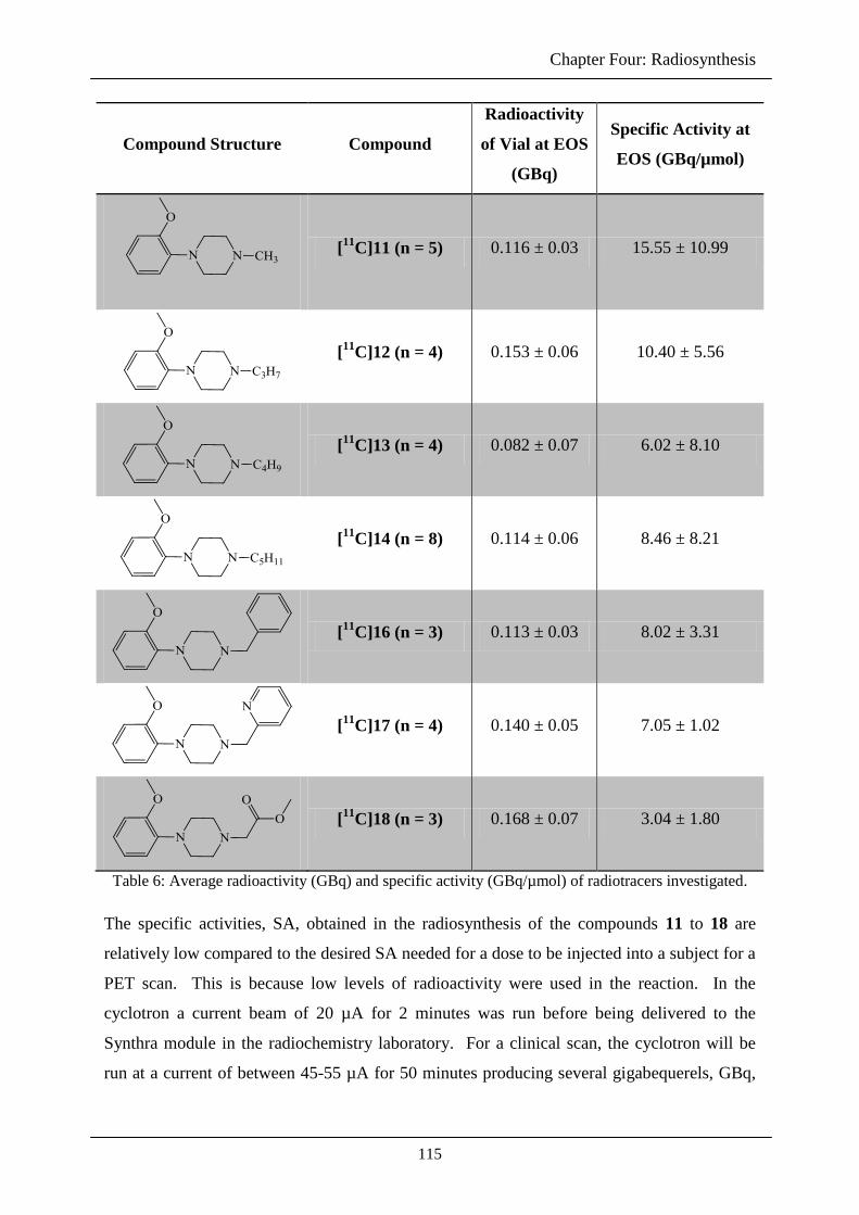
Chapter Four: Radiosynthesis
115
Compound Structure Compound
Radioactivity
of Vial at EOS
(GBq)
Specific Activity at
EOS (GBq/µmol)
[11
C]11 (n = 5) 0.116 ± 0.03 15.55 ± 10.99
[11
C]12 (n = 4) 0.153 ± 0.06 10.40 ± 5.56
[11
C]13 (n = 4) 0.082 ± 0.07 6.02 ± 8.10
[11
C]14 (n = 8) 0.114 ± 0.06 8.46 ± 8.21
[11
C]16 (n = 3) 0.113 ± 0.03 8.02 ± 3.31
[11
C]17 (n = 4) 0.140 ± 0.05 7.05 ± 1.02
[11
C]18 (n = 3) 0.168 ± 0.07 3.04 ± 1.80
Table 6: Average radioactivity (GBq) and specific activity (GBq/µmol) of radiotracers investigated.
The specific activities, SA, obtained in the radiosynthesis of the compounds 11 to 18 are
relatively low compared to the desired SA needed for a dose to be injected into a subject for a
PET scan. This is because low levels of radioactivity were used in the reaction. In the
cyclotron a current beam of 20 µA for 2 minutes was run before being delivered to the
Synthra module in the radiochemistry laboratory. For a clinical scan, the cyclotron will be
run at a current of between 45-55 µA for 50 minutes producing several gigabequerels, GBq,

Chapter Four: Radiosynthesis
116
of radioactivity. This increased amount of radioactivity leads to higher final specific
activities.
The mass of radiotracer synthesised during the reaction was consistent between runs and as
such it would be expected that with a large beam current and longer bombardment time in the
cyclotron, the radioactivity of the final radiotracer would be larger giving higher specific
activities. However, due to worker classification (as a student) it was not possible to use a
larger cyclotron beam which would lead to higher specific activities.
As the focus of this work is non-specific binding the autoradiography studies of each
radiotracer using rat tissue sections should not be affected by the low specific activities and
so it was not necessary to attempt to obtain higher values. This is because high concentration
solutions, ~100 nM, are used in order to ensure only non-specific binding is observed. This
means that there will be a high mass dose administered onto the rat tissue. In human PET
studies, high specific activities allow high amounts of radioactivity to be detected at target
sites while administering low doses of radiotracer (subnanomolar) meaning that there are
lower risks of toxicological and other side effects begin experienced by the human subject.
In rat tissue autoradiography, high mass doses of radiotracer should not affect the tissue or
results of the study as only non-specific binding is expected to be observed.
4.3 Conclusion
The successful radiosynthesis of compounds [11
C]11 – [11
C]14 and [11
C]16 – [11
C]18 using
[11
C]methyl iodide has been carried out. Radiochemical yields were good and showed that
the reaction had excellent efficiency. After separation on a semi-preparative HPLC, high
radiochemical purities were obtained and this allowed for the radiotracers synthesised to be
used in rat tissue autoradiography experiments as discussed in chapter 6. It was not possible
to obtain high specific activities due to low levels of radioactivity available for use in the
radiosynthesis reaction. With higher beam currents and beam times, specific activities would
be increased. However as radiotracers synthesised were not for clinical use it was decided
that the low specific activities were good enough as the mass of the radiotracer was consistent
between radiochemistry experiments.

Chapter Four: Radiosynthesis
117
4.4 Experimental
All precursors were used as synthesised in chapter two. All glassware, valves and tubing
used in the experimental were cleaned prior to use with acetone and ethanol and dried with a
stream of nitrogen and argon gas. All radiosynthesis work was carried out in the
radiochemistry laboratories at the GSK Clinical Imaging Centre at the Hammersmith
Hospital, London, UK. Radioisotopes were produced in a Siemens RDS-111 Eclipse
cyclotron and converted to [11
C]methyl iodide in a Synthra MEI (Boettcherkamp, Germany)
controlled by Synthra View version 5.04.043. Automated synthesis was carried out in a lead-
lined fumehood controlled using an in-house developed programme using the national
instruments Labview 7.1 software.
4.4.1 Synthesis of [11
C]11 – [11
C]14, [11
C]16 and [11
C]17 13
a) General Preparation
The relevant precursor (1 mg) was dissolved in a solution of DMF (500 µL) and 5M NaOH
(25 µL). Cyclotron-produced 11
CH3I was bubbled through the solution in a stream of helium
until a maximum reactivity had been reached and the vial was sealed. This was heated at 110
0C for 5 minutes before being quenched with HPLC eluent and loaded onto the HPLC loop
and purified on a C-18 reverse-phase semi-preparative HPLC using varying solvent
combinations of acetonitrile:water + 0.1% TEA at various flow rates (see table 4 for
individual compound separation conditions).
b) Synthesis of [11
C]18
1-(2-Hydroxyphenyl)-acetyl-piperazine, 9, (1 mg, 3.99 µmols) was dissolved in a solution of
DMF (500 µL) and Cs2CO3 (10 mg). Cyclotron-produced 11
CH3I was bubbled through the
solution in a stream of helium until a maximum reactivity had been reached and the vial was
sealed. The vial was heated at 110 0C for 5 minutes before being quenched with HPLC
eluent and loaded onto the HPLC loop to be purified using semi-preparative reverse-phase
HPLC and an isocratic mobile phase of acetonitrile:water +0.1% TEA (40:60) at a flow rate
of 5.00 ml/min.

Chapter Four: Radiosynthesis
118
4.5 References
1. H. R. Crane and C. C. Lauritsen, Int. Phys. Rev., 1934, 45, 497-498.
2. G. Antoni, T. Kihlberg and B. Langström, in Handbook of Radiopharmaceuticals:
radiochemistry and applications, eds. M. J. Welch and C. S. Redvanly, Wiley,
Chichester, Editon edn., 2003.
3. G. de Hevesy, Triangle, 1964, 91, 239-240.
4. B. Långström and H. Lunsqvist, Int. J. Appl. Radiat. Is., 1976, 27, 357-363.
5. T. Kniess, K. Rode and F. Wuest, Appl. Radiat. Isotopes., 2008, 66, 482-488.
6. P. Larsen, J. Ulin and K. Dahlstrom, J. Labelled. Compd. Rad., 1995, 37, 73-75.
7. P. Larsen, J. Ulin, K. Dahlstrom and M. Jensen, Appl. Radiat. Isotopes., 1997, 48.
8. T. Flessner and S. Doye, J. Prakt. Chem., 1999, 341, 186-190.
9. G. Dijkstara, W. H. Kruizinga and R. M. Kellogg, J. Org. Chem., 1987, 52, 4230-
4234.
10. Dictionary of Chemistry, 4 edn., Oxford University Press, Oxford, 2000.
11. M. E. Van Dort, J.-H. Kim, L. Tluczek and D. M. Wieland, Nucl. Med. Biol., 1997,
24, 707-711.
12. P. W. Miller, N. J. Long, R. Vilar and A. D. Gee, Angew. Chem. Int. Edit., 2008, 47,
8998-9033.
13. V. Gómez-Vallejo and J. Llop, Appl. Radiat. Isotopes., 2009, 67, 111-114.

CHAPTER FIVE:
MEASURING NON-SPECIFIC BINDING WITH
AUTORADIOGRAPHY

Chapter Five: Autoradiography
120
5.0 CHAPTER FIVE: MEASURING NON-SPECIFIC BINDING WITH
AUTORADIOGRAPHY
5.1 Introduction
In this chapter autoradiography techniques have been used to measure the non-specific
binding properties of the seven radioligands synthesised, as discussed in chapter 4, namely
[11
C]11, [11
C]12, [11
C]13, [11
C]14, [11
C]16, [11
C]17 and [11
C]18. After incubating rat tissue
sections with each radioligand, the non-specific binding was measured and the values
compared to selected physiochemical properties to form structure-activity relationships,
SARs. This was with the aim to make it possible to predict and have an understanding of a
particular compound’s non-specific binding properties and therefore it’s potential to behave
as a good radiotracer.
Autoradiography allows the distribution of radioactivity to be related to the detailed structure
of a specimen under investigation.1 It leads to a set of images recording the spatial
distribution and relationships of radioisotopes within a tissue specimen.2 In vivo
autoradiography involves injecting a radiolabelled drug into an animal. The radioligand
binds to the target receptor sites and the distribution of the receptors can be monitored using
PET technology. In vitro autoradiography generally uses fresh frozen tissue sectioned on a
cryostat and thaw-mounted on glass slides. These glass slides are then incubated in suitable
concentrations of the radioligand, washed and the slides opposed to radioisotope-specific
media, a length of time allowed to elapse, followed by analysis of each slide onto
radiograms.1
Autoradiography is a highly specific tool available for analysing and characterising biological
receptors. It provides locatisation of proteins of interest in tissues samples and enables the
characterisation of these proteins in different tissues, brain regions and/or animal samples.
However the presence of a high-affinity receptor radioligand does not mean that the receptor
has physiological significance and it can be difficult to truly determine whether the binding
site actually corresponds to the actual receptor, without the means ofdelineating the specific
binding component of the radioligand from that which is non-specifically bound.
Due to the nature of the PET radioisotope utilised in these studies, namely carbon-11, a
phosphor storage system was adopted for use in the autoradiography experiments reported in
this chapter rather using traditional film autoradiography that detects tritiated radioligands.

Chapter Five: Autoradiography
121
Phosphor storage screens capture and store the radioactivity from a sample which is exposed
in cassettes. The imaging plate consists of photostimulable phosphors which detect and store
accumulated ionising radiation. On excitation of the phosphor by a laser beam, the stored
energy is released as luminescence which is digitised to form a quantitative image of the
sample. The intensity of the luminescence is proportional to the intensity of the radioactivity
detected by the phosphor screen.3
Phosphor storage autoradiography has many advantages over the traditional film
autoradiography method, the most important being the rapid speed at which an image can be
captured and quantified compared with conventional tritiated autoradiography. The phosphor
screens that are used to detect the radioactivity in the sample are also reusable further lending
to their beneficial utility. This technique is rapid and several screens/cassettes can be utilised
simultaneously and left until it is possible to scan the image. The short scan time for each
phosphor screen also allows for multiple screens to be recorded over the course of a day.
However, the resulting images exist only as an electronic files and print outs and re-scanning
the screen in an individual experiment can, lead to a loss in resolution and artefacts appearing
in the final image.4
The in vitro labelling of slide-mounted tissue sections is a widely used method for measuring
the binding of radioligands in tissue samples. Over the last couple of decades developments
in this technique have led to improvements in analysis, image quality and image
quantification making it a simpler and more suitable experimental method for the
measurement of radioligand binding.
5.2 Methodology
A simple autoradiography technique was used to measure in vitro the binding of radiolabelled
compounds [11
C]11, [11
C]12, [11
C]13, [11
C]14, [11
C]16, [11
C]17 and [11
C]18, as discussed and
synthesised in chapter 5, in rat brain tissue sections.
Male Wistar rat brains were sectioned using a cryostat (CM3050S Leica, UK) and the
sections were thaw-mounted on to gelatine-coated glass slides, figure 1, A). Rat brains were
section in the sagittal plane (20 µm thickness, according to the atlas of Paxinos and Watson,
1998) in order to see binding across all regions in the brain and allow the cerebellum to be
present in each section. This is important as the cerebellum can be used as a reference region
in particular binding studies where this region of the brain is found to be reasonable devoid of

Chapter Five: Autoradiography
122
the protein target under investigation. Ultimately this would then allow for the delineation
and estimation of the specific binding component of the radioligand under investigation
versus the non-specific binding component.
Figure 1: Schematic to show the experimental steps during the autoradiography experiments; A) tissue
section placed on gelatin-coated glass slide; B) tissue section incubated in Tris-buffer containing
radioligand; C) tissue section removed and washed before analysis of the bound radioligand.
The seven carbon-11 radioligands were synthesised at GSK Clinical Imaging Centre
(Hammersmith, UK). Each radiosynthesis occurred on the day of the autoradiography study.
Tissue sections were removed from the freezer, 2 slides per incubation time point (6 time
points; total = 12 slides per experiment) with 3 tissue sections per slide. Slides were washed
in cold Tris-buffer (50 mM, pH 7.4, 4 oC) for 15 minutes. During this time the incubation
solution was made up using Tris-buffer (50 mM, pH 7.4, 21 oC) and the required volume of
[11
C]radioligand to make a final concentration of 100 nM in the buffered solution.
For each experiment conducted there was a variation in the concentration of the radioligand.
It was difficult to radiosynthesise each production of radioligand to the same radioligand
mass concentration with a suitable radioactivity level that would allow for a solution to be
formulated at a final concentration of 100 nM. Low specific activities were achieved for
some radioligands, as discussed in chapter 4, making it difficult to always have a
concentration of 100 nM and a high radioactivity in every individual experiment. It was
sometimes necessary to have a very high concentration of the radioligand, 1 µM in order to
have enough radioactivity to be detected. Some experiments were carried out at lower
concentrations and this is discussed further in section 5.3.
Once the Tris-buffer and [11
C]radioligand solution was at the desired concentration, slides
were incubated for 3, 8, 14, 20, 30 and 40 minutes, figure 1, B) (2 slides per time point = total
of 6 sections). A time-course study was conducted for each radioligand in order to determine
A) B) C)
Rat tissue Section
[11
C] Radioligand Solution
Rat tissue Section with
[11
C] radioligand bound

Chapter Five: Autoradiography
123
that the binding of each [11
C]radioligand had reached equilibrium within the 40 minute time
period.
After incubation, tissue sections were washed twice in cold Tris-buffer (50 mM, pH 7.4, 4
oC) and once in ice-cold distilled water (4
oC) to remove unbound [
11C]radioligand and salts
that could cause artefacts in the final analysis, figure 1, C). Slides were dried in a cool
airstream, (which can help minimise the diffusion of the radioligand and prevents denaturing
of the protein which can occur at higher temperatures) and were exposed to carbon-11
sensitive phosphor screens (Amersham, UK) with [11
C]radioligand standards.
[11
C]Radioligand standards (5 µL) at 100, 50 and 10 nM were pipetted onto tissue attached to
a glass slide, allowed to dry, and exposed to the phosphor screen with the tissue sections.
Figure 2: A) Photograph of the tissue sections (two slides per incubation time point) with radioligand
standards, and B) an example of the image obtained from the autoradiographic phosphor screen.
Tissue sections were exposed to a phosphor screen overnight in order to allow the carbon-11
to decay prior to image capture using the cycloneTM
storage phosphor system (Packard,
Perkin Elmer) and OptiQuant (version 5.0, Perkin Elmer) giving a greyscale image of the
radioligand bound to the tissue section, figure 2. The image given in figure 2 was analysed
using MCID Core 7.0 (GE Healthcare Niagara Inc) program. The [11
C]radioligand standards
A) B)
[11
C]Radioligand Standards at 100, 50, 10 nM

Chapter Five: Autoradiography
124
were used to form calibration curves which allowed the quantification of the amount of
radioligand bound in the following regions of interest: cerebellum, motor cortex, caudate
putamen and the whole brain (comprising of an average of 28 points across the whole brain
section), figure 3.
A)
B)
Figure 3: A) Schematic representation to show the various brain regions investigated. The whole brain
(black outline) region was an average of 28 points across the whole section. B) Map of the sagittal
brain section showing important regions including the cerebellum (CM), caudate putamen (CP) and
Motor cortex (C), taken from Jarvis et al.5
The amount of radioligand bound in each region of interest was converted to a relative
percentage of the total amount of radioligand available to bind to the entire tissue section and
quoted as non-specific binding percentage, NSB %. Any binding associated with any of the
radioligands to the tissue sections was assumed to be all non-specific binding as the
radioligands under investigation had not been synthesised to bind to a specific protein target
site.
Autoradiography experiments for [11
C]11, [11
C]12, [11
C]13, [11
C]14, [11
C]16, [11
C]17 and
[11
C]18 were repeated using tissue sections obtained from four different rat brains. All data
was analysed using the iterative non-linear regression curve fitting software (GraphPad Prism
5.0), fitting the data to one-site models of binding. Data are expressed as mean ± s.e.mean.
Cerebellum Motor Cortex
Caudate
Putamen

Chapter Five: Autoradiography
125
5.3 Results and Discussion
For the radioligands under investigation, it was expected that any binding to the rat tissue
would be non-specific as these radioligands were not generated for a specific protein target
site. As a result, the amount of bound radioligand is quoted as a non-specific binding
percentage, NSB %, and all values and graphs use this notation, unless otherwise stated.
5.3.1 Time-course Experiments
It is important when investigating non-specific binding to measure the binding of the
radioligand once the system has reached equilibrium. Time-course experiments were
conducted for each radioligand to determine whether binding equilibrium would be reached
over a 40 minute incubation time. Binding, recorded as the NSB %, was measured in tissue
sections at 3, 8, 14, 20, 30 and 40 minutes and the data fitted to a one-site binding model,
figure 4. The whole brain NSB % for each rat experiment (i.e. n = 4) is an average of 6 rat
tissue sections. For each section, 28 individual points were measured across the whole brain
section and averaged. Each experiment NSB % was an average of the 6 rat sections and the
standard errors of mean were calculated where n = 4.

Chapter Five: Autoradiography
126
0 10 20 30 400
25
50
75
100
NSB (%) [11C]12 NSB (%) [11C]13
NSB (%) [11C]16 NSB (%) [11C]17 NSB (%) [11C]18
NSB (%) [11C]14NSB (%) [11C]11
Time (mins)
NS
B (
%)
Figure 4: Graph to show the average NSB % for rat whole brain over a period of 40 minutes
and a radioligand mass concentration range of 1 – 1000 nM (n=4).
Figure 4, shows for all of radioligands, except [11
C]13, the NSB % reached a plateau by 20
minutes, indicating that equilibrium was reached by this time. Radioligand [11
C]13 was the
only compound that did not reach an equilibrium by 20 minutes. However it would have
been unfavourable to increase the incubation period beyond 40 minutes since the carbon-11
half life is 20.4 minutes and the experiment alone used two half-lives. If a longer
experimental time was used, the radioactivity would decay too much during the course of the
experiment, and would make analysis of the final image difficult as too little radioactivity
would be able to be detected by the phosphor screen. Therefore, since all the other
radioligands had reached equilibrium within the 40 minute incubation period it was decided
not to extend this time to assess the potential equilibrium of radioligand, [11
C]13.

Chapter Five: Autoradiography
127
The graph in figure 4 shows the average NSB % for all experiments carried out, where n = 4.
However experiments were not always conducted at the same radioligand mass concentration
due to the variation in specific activities achieved for each independent [11
C]radioligand
synthesis. For a true comparison of the NSB % data it is important to use experiments where
the concentration of [11
C]radioligand was at 100 nM, see figure 5.
0 10 20 30 400
25
50
75
100
NSB (%) [11C]11 NSB (%) [11C]12 NSB (%) [11C]13 NSB (%) [11C]14
NSB (%) [11C]16 NSB (%) [11C]17 NSB (%) [11C]18
Time (mins)
NS
B (
%)
Figure 5: Graph to show the average NSB % over a period of 40 minutes and a radioligand
mass concentration of 100 nM for the whole brain region (n = 2).
For several of the [11
C]radioligands it was only possible to get one rat brain tissue
autoradiography experiment measured at 100 nM ([11
C]11, [11
C]13, [11
C]14, [11
C]17 and
[11
C]18). Where more than one rat autoradiography experiment was conducted for a
particular radioligand at 100 nM, errors have been included on the graph, figure 5. At a fixed
concentration of 100 nM equilibrium was reached in 20 minutes for all radioligands,
including [11
C]13, figure 5, and it can also be noted that radioligands [11
C]13 and [11
C]16
have NSB % values above 45 % post 20 minutes while all other radioligands have a NSB %
value below 25 %. The NSB %, measured at 40 minutes will be used to compare to each

Chapter Five: Autoradiography
128
physicochemical property forming the structure-activity relationships. Between figures 4 and
5 everything remains the same in terms of NSB % for each radioligand except for [11
C]14.
For this radioligand the NSB % drops to 25 % in figure 5 compared to the 60 % it was in
figure 4. This is due to the removal of errors caused by inconsistent radioligand mass
concentrations used to generate the curve for this radioligand in figure 4.
5.3.2 Possibility of specific binding
From the data given in figure 5, it can be observed that a similar pattern of NSB % was
observed for all radioligands in terms of reaching equilibrium by 20 minutes. However when
comparing the binding of each radioligand to the regions-of-interest it could be seen that
there may be a degree of specific binding for some of the radioligands.
Using the autoradiography data plotted against time for each region of interest, figure 6,
radioligands with possible specific binding can be observed. When comparing the raw data
for the cerebellum brain region and the motor cortex and caudate putamen, it can be seen that
for compounds [11
C]11, [11
C]13 and [11
C]16, there was a greater than 9 % difference between
the NSB %, suggesting that these two compounds may display a degree of specific binding to
a target protein in the rat brain section. For radioligands [11
C]12, [11
C]14, [11
C]17 and
[11
C]18 it can be seen they have NSB % of approximately 6 % greater in the motor cortex or
caudate putamen when compared to the cerebellum region of interest. However statistical
analysis has suggest different radioligands have a possible degree of specific binding to an
unknown protein target within in the ROIs. It is important to note that the statistical analysis
was carried out using data with n = 1.
Statistical analysis of the data obtained in the autoradiography experiments was carried out
using GraphPrism® v.5 using an extra sum-of-squares F test to obtain the P value for the data
with the convention that alpha = 0.05 whereby a result that is said to be significantly
significant when a difference greater than that would occur 95 % of the time if in the
populations were identical. Therefore if the P value is below 0.05, the result is significant
and the data is different for all data sets, and if the P value is above 0.05 the result is not
significant and the data is the same for all data sets.

Chapter Five: Autoradiography
129
Figure 6: Graphs to show the time-course uptake of radioligands in each region of interest, whole
brain (red), cerebellum (blue), motor cortex (green) and caudate putamen (pink) at 100 nM.
[11
C]11 [11
C]12
[11
C]13 [11
C]14
[11
C]17
[11
C]18
[11
C]16
7

Chapter Five: Autoradiography
130
From statistical analysis carried out on the data of each radioligand, it was seen that [11
C]12
(P = 0.33), [11
C]16 (P = 0.44) and [11
C]18 (P = 0.94) had no statistical significance and it is
unlikely any difference of NSB % between ROIs is due to potential specific binding to an
unknown target protein. It is more likely the difference is due to errors within the data.
Radioligand [11
C]16 was seen to have no statistical significance suggesting that the curves for
each ROI were the same and any difference observed between each ROI is likely due to error.
However images recorded during the autoradiographical experiments indicated higher uptake
of radioligand (higher density of radioactivity detected on phosphor plate) in various ROIs
suggesting there could be some degree of specific binding. There was also a large difference
between the cerebellum and the motor cortex and caudate putamen NSB % at 40 minutes
incubation, 15 % difference, which could also suggest there is a degree of specific binding
associated with these regions.
Radioligand [11
C]11 has a very large statistical significance (P < 0.0001) and alongside the
autoradiographical images recorded during the experiments, it can be assumed there is a
degree of specific binding that may affect the NSB % measured at 100 nM.
When a statistical analysis was carried out on the data for radioligands [11
C]13 (P = 0.04),
[11
C]14 (P = 0.01) and [11
C]17 (P < 0.0001) it was noted that there was statistical significance
between each of the ROIs indicating a possibility that these radioligands experience a degree
of specific binding.
All radioligands used in the autoradiograpical experiments were expected to only have non-
specific binding however it has been seen both within images recorded during the experiment
and by differences between NSB % measured in ROIs that there is a possibility that several
of the radioligands will have a degree of specific binding to an unknown protein target. With
this in mind it is important use a reference region in order to obtain a NSB % for each
radioligand to allow SARs to be drawn. The cerebellum has previously been used as a
reference region in autoradiography experiments for some radioligands, as the cerebellum
region was reasonably devoid of the protein target under investigation.6, 7
Radioligand [11
C]13 showed there was a difference between the cerebellum and the motor
cortex at 100 nM, however this was only a small difference and images recorded appeared to
demonstrate relatively homogenous binding of [11
C]13 across the tissue sections, figure 7B.
Interestingly the NSB % of [11
C]13 was also measured at 1 µM, figure 7A.

Chapter Five: Autoradiography
131
When the autoradiography image for [11
C]13 was developed at 1 µM, it appeared there was a
larger uptake of this radioligand in the motor cortex, caudate putamen and the hippocampus,
up to 14 minutes post-adminstration, figure 7A. At 40 minutes incubation there was over 20
% more binding measured in the motor cortex and caudate putamen than in the cerebellum.
This suggests at higher concentrations there is a greater amount of potential specific binding
than at the lower 100 nM mass concentration.
3 mins 8 mins 14 mins
a) 20 mins 30 mins 40 mins
3 mins 8 mins 14 mins
b) 20 mins 30 mins 40 mins
Figure 7: Autoradiographical images recorded for radioligand [
11C]13 when the NSB % measurement
was carried out at a) 1 µM and b) 100 nM. Motor cortex (MC), hippocampus (Hi), caudate putamen
(P), meduilla (Me) and cerebellum (Ce).
Radioligand [11
C]11 represents one of the compounds in this series that showed the
possibility of exhibiting a degree of specific binding in some of the ROI’s measured from the
autoradiographical experiments.
P
MC Hi
Me
Ce

Chapter Five: Autoradiography
132
For radioligand [11
C]11 a larger difference of 16 % between the cerebellum reference region
and the motor cortex was observed, figure 6. A small difference was also observed between
the cerebellum and caudate putamen suggesting there could be a small specific binding
component associate with this region compared to the motor cortex. The autoradiographical
images in figure 8 clearly show the motor cortex region leading to the belief there could be a
specific binding component of [11
C]11 associated with this region. There was also a larger
amount of uptake in the hippocampal compared with the cerebellum, however this region was
not analysed independently as a separate ROI.
3 mins 8 mins 14 mins 20 mins 30 mins 40 mins
Figure 8: Autoradiographical images recorded for radioligand [
11C]11 when the NSB % measurement
was carried out at 100 nM. Motor cortex (MC) and hippocampus (Hi).
Due to the high mass concentrations of each radioligand used in each of the autoradiography
experiments (100 nM) it was not expected that any specific binding would be observed.
However, for several radioligands it has been observed that an element of unconfirmed
specific binding may be present in the motor cortex, caudate putamen and hippocampus. If
specific binding is truly being observed in these regions, it is most likely that each
radioligand is binding to similar receptors within each of the ROI due to the similar
piperazine moiety these radioligands share with one another.
5.3.3 Possible Receptors to which the radioligands may Bind
It was not possible to conduct experimental competition binding studies to assess the target
proteins to which these radioligands may bind. However, the structure of the radioligand and
knowledge of which receptors/target proteins are present in each ROI can be used to suggest
possible binding targets.
There are several compounds in the literature containing a similar piperazine moiety to the
radioligands synthesised in this work. They have been synthesised to investigate their
binding properties to various receptor types. Arylpiperazines are considered a versatile
template for synthesising compounds that can act at the serotoninergic, adrenergic and
dopaminergic receptors.6
MC Hi

Chapter Five: Autoradiography
133
Several of the arylpiperazine compounds have shown large affinities for the serotonin
receptor, 5-HT1A. This receptor system is important in the neurotransmission network
regulating physiological and behavioural functions.7 The 5-HT1A receptor is involved in
anxiety, depression and schizophrenia 8 and in particular receptor antagonists could be useful
in treating cognitive disorders such as Alzheimer’s disease.9 These types of receptors are
usually found in high concentrations in the hippocampus, layers of the cortex, the caudate
putamen and the raphe nuclei.10
Mokrosz et al.11
has investigated the effect of an alkyl chain in an arylpiperazine compound
and their affinities with the 5-HT1A receptor. In this study, it was seen that increasing the
alkyl chain length, 2-6 carbons, in the molecule enhanced the 5-HT1A affinity. It was also
seen that the alkyl substituents enhanced the 5-HT2/5-HT1A selectivity ratio. It was suggested
that the alkyl chain could be accommodated at the receptor and the bioactive complex may be
stabilized by hydrophobic interactions. The compounds discussed by Mokrosz and co-
workers 11
have a similar structure to the radioligands discussed in this thesis.
Radioligand [11
C]11 showed increased up-take in the motor cortex and hippocampus which
are regions both known to contain 5-HT1A receptors. As several compounds with a similar
structure bind to this receptor it would be predicted that this radioligand may also bind to this
subtype of the 5-HT receptors.
A similar compound to the radioligands synthesised in this work is the compound WAY-
100635 which contains the same 1-(2-methoxyphenyl)piperazine group, figure 8 chapter 1. It
is well detailed that WAY-100635 has good in vitro affinity for 5-HT1A receptors 12, 13
and
good selectivities against the 5-HT2 receptor.14
It has also been shown that WAY-100635 has
a modest potency towards dopamine receptors. Martel et al.15
showed that WAY-100635 has
a high potency for blocking 5-HT1A receptors but also has a modest potency and efficacy for
activating dopamine D4 receptors. Radioligands in this work showing a degree of specific
binding could have similar characteristics to WAY-100635 whereby it binds and acts on the
5-HT1A receptors which can be seen by the up-take in the motor cortex, hippocampus and
caudate putamen. While it can also affect the dopamine receptors as seen by increased up-
take in the cerebellum.
WAY-100635 is not the only arylpiperazine compound to show some affinity to the
dopamine receptors. Several compounds containing this moiety have been synthesised,
radiolabelled and investigated to understand their affinity to the dopamine receptors.16-18

Chapter Five: Autoradiography
134
Dopamine receptors have two sub-types D1, containing D1A, D1B and D5, and D2, containing
D2, D3 and D4 receptor types. There are more D1 binding sites than D2 and the highest
concentration of D1 receptors can be found in the caudate putamen, olfactory tubercle amd
substantia nigra. There is a moderate concentration of D1 receptors in the cerebellum and in
rat tissue, D2 receptors can be found in the caudate putamen.19
From the autoradiographical images radioligand [11
C]16 showed possible specific binding in
the motor cortex, caudate putamen and cerebellum when studying the images recorded during
each experiment. These regions are known to contain (amongst other protein targets), 5-
HT1A receptors, which may represent a potential target protein accounting for potential
specific binding observed for this radioligand. However, what appears to be an element of
specific binding of [11
C]16 was also visualised in the cerebellum suggesting that this
radioligand may bind to another target protein present in this region. Petterson et al.20
has
shown that 3-(1-benzylpiperadin-4-yl)phenol, the phenol derivative of [11
C]16, demonstrates
a high preference for the activated state of the D2 receptor. It was suggested that the phenol
group, anilinic nitrogen and large N-alkyl group stabilize the dopaminergic receptors.
Radioligand [11
C]16, although does not contain a phenol group, could have similar properties
to this derivative and may also display a degree of specific binding to the D2 receptor.
If the radioligands in this work are truly binding specifically to a protein target in the rat
brain, the obvious candidate protein for this binding are the 5-HT1A receptors, however this
would need to be definitively demonstrated. Blocking studies using unlabelled compounds
which target each of these specific receptor types should be conducted to determine exactly
which proteins the radioligands are binding. These studies were, unfortunately, beyond the
scope of work conducted for this thesis.
5.3.4 Non-specific Binding % using Cerebellum Data
Because some of the radioligands still exhibited small amounts of specific binding in various
brain regions even at 100 nM concentrations, it was decided to use the radioligand data
measured in the cerebellum as the measure of non-specific binding, NSB %. The cerebellum
is regularly used as a reference region when the target protein of interest is not expressed in
this region. The NSB % for each radioligand against incubation time (i.e. a time-course), was
plotted in order to show (1) the uptake of each radioligand into the cerebellum and (2) time to
reach equilibrium, determined by the curve reaching a plateau, figure 9.

Chapter Five: Autoradiography
135
0 10 20 30 400
25
50
75
100
NSB (%) [11C]11 NSB (%) [11C]12 NSB (%) [11C]13 NSB (%) [11C]14
NSB (%) [11C]16 NSB (%) [11C]17 NSB (%) [11C]18
Time (mins)
NS
B (
%)
Figure 9: Time-course to show the uptake of each radioligand in the cerebellum at 100 nM.
Using the cerebellum as a reference region for determination of the NSB %, any specific
binding present in other brain regions which will increase the whole brain non-specific
binding average will be reduced. This will make the non-specific binding % between each
radioligand more comparable. The time-course for each radioligand at 100 nM was recorded
over a 40 minute incubation period. Figure 9 demonstrates a similar appearance to that using
the whole brain data, figure 5.

Chapter Five: Autoradiography
136
Radioligand Whole Brain NSB % Cerebellum NSB %
[11
C]11 19.32 10.91
[11
C]12 15.92 13.00
[11
C]13 51.54 44.43
[11
C]14 25.50 22.49
[11
C]16 79.68 71.37
[11
C]17 10.27 7.86
[11
C]18 6.60 7.61
Table 1: Table to summarise the NSB % measured in the rat whole brain and the cerebellum using a
fixed concentration of 100 nM for each radioligand following a 40 minute incubation.
Across the 7 radioligands assessed, there was a large range of NSB % observed for the
cerebellum (ranging from 7.61 to 71.37 %, Table 1) which may reflect the differences in
chemical structures between these compounds, thereby influencing the degree of NSB %
exhibited by each radioligand. In order to interpret each radioligand’s true NSB %
characteristics it is important to remove any specific binding component associated with that
radioligand, hence the use of the cerebellum as a potential reference region. It must be
considered, however, that the cerebellum is a region that has been utilised as a reference
region for particular radioligands due to the region being reasonably devoid of the proteins
under investigation. Therefore the use of the cerebellum as a reference region in the studies
reported here should be treated with an element of caution in case the radioligands bind to a
target protein located in this region.
From the autoradiographical experiments outlined in this chapter, the cerebellum uptake at
the radioligand concentration of 100 nM at 40 minutes has been assumed to provide the NSB
% for each radioligand under investigation. The NSB % obtained from the cerebellum region
under the above conditions has been used to produce the structure-activity relationships
between each physiochemical parameter discussed in chapter 3.
5.4 Structure-Activity Relationships
In chapter 3 the physicochemical parameters that have been suggested to have an effect in the
non-specific binding properties of a radioligand were discussed. These included (1) the
lipohilicity of the compound, (2) CHI_IAM, (3) the acid dissociation constant, (4) the
interaction energy and (5) molecular weight. Each of these properties has been compared
with the NSB % obtained from the measurement of the cerebellum as quoted in table 1.

Chapter Five: Autoradiography
137
5.4.1 Lipophilicity
In this work CHI_Log D at pH 7.4 was used as the measure of lipophilicity as it is a
distribution coefficient dependent on pH, as discussed in chapter 3. In vivo Log D is the
preferred measure of lipophilicity as it considers all unionised and ionised forms of the
molecule at the chosen pH.
The NSB % for the cerebellum was plotted against the CHI_Log D7.4 for each radioligand, in
order to determine the structure-activity relationship between the two parameters, figure 10.
Figure 10: Graph to show the relationship of NSB % with changing lipophilicity, CHI_Log D7.4
It can be seen that when the CHI_Log D7.4 is above 3 the NSB % is high. The correlation
between the data gives an r2 = 0.69 which was not a good correlation. However, the higher
NSB % at CHI_Log D7.4 above 3 followed what has previously been stated in literature.21
The radioligand [11
C]13 could represent an outlier in the data set and would suggest that the
NSB % of a compound may not be able to be predicted from the lipophilicity alone, but
requires other physiochemical parameters to be determined before predicting the final non-
specific binding properties that a radioligand may possess.
Several radioligands have been predicted to demonstrate an element of specific binding from
the autoradiography experiments. It is also possible to get specific binding in the cerebellum
brain region and the non-specific binding value for these radioligands could lead to a skew in
11 12
13
14
16
17 18
R² = 0.6947
0
10
20
30
40
50
60
70
80
0 0.5 1 1.5 2 2.5 3 3.5 4
Non
-sp
ecif
ic B
ind
ing (
%)
Lipophilicity, CHI_Log D7.4

Chapter Five: Autoradiography
138
the relationship between CHI_Log D7.4 and non-specific binding. This could be causing
difficulties when determining a correlation between the two parameters.
It is difficult to obtain a relationship between CHI_Log D7.4 and non-specific binding from
the data obtained in this work. In previous literature, correlations between these two
parameters have also been low and large numbers of data points have been required to obtain
a good enough correlation to see the relationship.22
5.4.2 Immobilised Artificial Membrane, CHI_IAM
It would be expected that the CHI_IAM and CHI_Log D7.4 would give a similar relationship
regarding non-specific binding since they rely on similar physicochemical properties. The
CHI_IAM is a measure of how a compound may bind to a cell membrane. The CHI_IAM
uses an immobilised artificial membrane to measure this value. This means the CHI_IAM
has the ability to mimic, in part, a biological cell membrane, whereas the CHI_Log D7.4
measures the partition of the compound between an organic and aqueous phase.
The CHI_IAM is an important physicochemical parameter and positively charged molecules
usually show higher partition to the membrane binding more strongly to the phospholipids.
The CHI_Log D7.4 does not distinguish between the negative and positive charges in a
molecule and as such the CHI_IAM is an interesting parameter to use for the prediction of
non-specific binding properties. On comparison of the CHI_IAM and CHI_Log D7.4 it can be
seen in figure 11, that the correlation between both parameters is low whereas in literature
comparisons such as this have shown positive linear correlations.27

Chapter Five: Autoradiography
139
Figure 11: Graph to show the relationship between the CHI_Log D7.4 and CHI_IAM values obtained
on an IAM stationary phase.
The CHI_IAM was plotted against the NSB % for the cerebellum for each radioligand, in
order to determine the structure-activity relationship between the two parameters, figure 12.
It can be seen that generally when the CHI_IAM is below 37, the NSB % is below 20 %.
Figure 12: Graph to show the relationship of NSB % with changing CHI_IAM.
A low CHI_IAM is seen to give low non-specific binding which increases as the CHI_IAM
increases. A correlation between both parameters can be produced with a low r2 value and
removal of compounds showing potential specific binding in order to show a relationship
R² = 0.4285
0
10
20
30
40
50
60
0 1 2 3 4 5 6
CH
I_IA
M
CHI_Log D7.4
11 12
13
14
16
17 18
R² = 0.4126
0
10
20
30
40
50
60
70
80
15 20 25 30 35 40 45
Non
-sp
ecif
ic B
ind
ing (
%)
CHI_IAM
Chapter Five: Autoradiography
140
between CHI_IAM and true NSB may give a great correlation between the data. Recent
work by Jiang et al. 23
has shown that as the CHI_IAM increases, the NSB % also increases
giving a linear relationship between the two with a high correlation r2 = 0.79. A similar
relationship has been shown in this work.
From the data obtained in this work and previous publications, it can be seen that the
CHI_IAM of a radioligand could be a better predictor to its non-specific binding properties of
a ligand than the CHI_Log D7.4 alone. The CHI_IAM of a radioligand is rarely calculated or
quoted in the literature. However the CHI_IAM is measured in order to see how a compound
will act on the surface of a cell membrane. This means the CHI_IAM could be more
representative of how the compound will act in vivo than the CHI_Log D7.4. To date little
work has been conducted to investigate whether the CHI_IAM could represent a key
parameter in predicting non-specific binding. Therefore data from other radioligands with
known non-specific binding values should be collected in future studies.
The results of this work suggest that factors other than lipophilicity alone are contributing to
the phenomenon of non-specific binding.
5.4.3 Acid Dissociation Constant, pKa
The acid dissociation constant, pKa, has been suggested to affect the rate of membrane
hydrolysis in a cell bilayer. Within the literature hydrolysis of giant unilamellar vesicles was
seen to occur in a 35 minute time period and as such measuring NSB % at 40 minutes should
allow hydrolysis of the lipid bilayer to have begun. It has been predicted that as the pKa of a
compound increases, the hydrolysis rate will decrease due to the compound being a weaker
acid, therefore the non-specific binding will be increased with high pKa values.

Chapter Five: Autoradiography
141
Figure 13: Graph to show the relationship of NSB % with changing acid dissociation constant, pKa.
The structure-activity relationship, SAR, between pKa and NSB % for compounds [11
C]11,
[11
C]12, [11
C]16, [11
C]17 and [11
C]18 is given in figure 7. Data for [11
C]13 and [11
C]14 have
been omitted because their pKa values were not measured in this work as discussed in
chapter 3. There was little correlation observed between the two parameters. Figure 13
shows all the radioligands, except [11
C]16 gave NSB % below 15 % which suggests these
radioligands may have the potential to be good radioligands. [11
C]16 demonstrated a high
NSB % of over 70 % which has the possibility of skewing the data. From this SAR it could
be concluded that the pKa of a compound has little effect on the non-specific binding.
However, it does suggest that other parameters need to be considered when predicting non-
specific binding. It is important to look at all the physicochemical properties of a radioligand
to determine whether it will be a good radioligand. It is difficult to conclusively state the true
relationship seen in figure 13 and further non-specific binding values are need to be measured
experimentally to determine the true relationship.
5.4.4 Interaction Energy
The interaction energy, kcal/mol, was computationally measured for all the radioligands to
determine the lowest energy required for a single lipid to associate with a single radioligand
molecule, figure 14. It was predicted that as the interaction energy decreases (becomes more
positive) the lower the non-specific binding will be since compounds will either cross the
bilayer rapidly or not at all, further discussed in chapter 3.
18 17
16
12 11
0
10
20
30
40
50
60
70
80
5 5.5 6 6.5 7 7.5 8 8.5 9
Non
-sp
ecif
ic B
ind
ing (
%)
Acid Dissociation Constant, pKa

Chapter Five: Autoradiography
142
Figure 14: Graph to show the relationship of NSB % with changing interaction energy, kcal/mol.
It can be seen from the non-specific binding data collected during the autoradiographical
experiments, that as the interaction energy becomes stronger (becomes more negative) the
non-specific binding decreases, figure 14. This is the opposite relationship to what has been
determined previously in literature.22, 24
It is important to note that in literature the 20
radiotracers investigated have interaction energies in the range of -5 to -20 kcal/mol. When
comparing the data obtained in this work where the interaction energies lie in the range of -1
to -3.5 kcal/mol, the data is going to be slightly noisy and a relationship between the two
parameters will be difficult to determine.
In this work there are fewer data points and several radioligands may experience a degree of
specific binding leading to the belief that the lower the interaction energy the higher the non-
specific binding.
11
12
13
14
16
17 18
0
10
20
30
40
50
60
70
80
-3.5 -3 -2.5 -2 -1.5 -1
Non
-sp
ecif
ic B
ind
ing (
%)
Interaction Energy (kcal/mol)

Chapter Five: Autoradiography
143
5.4.5 Molecular Weight
It is understood that compounds with low molecular weights, i.e. below 500 MW, generally
yield good drug molecules.25
It has been predicted that the smaller the molecule, the more
able it is to cross the lipid bilayer and therefore have a lower non-specific binding.
Figure 15: Graph to show the relationship of NSB % with changing molecular weight.
Figure 15, indicates that the radioligands assessed in this study possessed a molecular weight
below 300 and yielded low non-specific binding, with the exception of radioligands [11
C]13
and [11
C]16. The reason for these outliers is the possibility that they have a specific binding
component that increases the NSB %. For these two compounds, it would be important to do
a competitive binding study and determine the true non-specific binding value before re-
plotting this data to confirm that radioligands with molecular weight below 500 can have low
non-specific binding. Generally the non-specific binding for the radioligands measured is
low and it follows the rule-of-five set out by Lipinski et al.25
that when the molecular weight
is below 500, blood-brain barrier (BBB) permeability is good and NSB is low.
It is important to consider the other physicochemical properties when predicting non-specific
binding of a radioligand. Parameters such as lipophilicity and CHI_IAM appear to have a
greater effect on the non-specific binding of a radioligand and as such the molecular weight
has less importance when looking at single properties as predictors for non-specific binding.
However, the molecular weight of a molecule will have an effect on its lipophilicity, for
example, if a large alkyl chain is added to a compound, the molecular weight will be
increased as well as its lipophilicity. This means indirectly, molecular weight can have an
11 12
13
14
16
17 18
0
10
20
30
40
50
60
70
80
200 220 240 260 280 300
Non
-sp
ecif
ic B
ind
ing (
%)
Molecular Weight

Chapter Five: Autoradiography
144
influence on non-specific binding, even it is does not necessarily directly affect it. As such, it
is important to consider this parameter when in the initial stages of drug design along with
each of the other physiochemical properties discussed.
5.5 Conclusion
The up-take and non-specific binding of each radioligand synthesised has been successfully
carried out in autoradiographical experiments using rat brain tissue. The binding of each
radioligand across the whole brain section has been measured as well as measuring the uptake
in the cerebellum, motor cortex and caudate putamen. Time-course experiments showed
equilibrium was reached rapidly for all radioligands by 20 minutes, however it was decided
to use the NSB % values measured at 40 minutes to determine the structure-activity
relationships. This allowed for the comparison of the NSB data with the data obtained in the
mass spectrometry cell assay discussed in chapter 6.
Unexpectedly specific binding was observed for some of the radioligands, and as such the
non-specific binding measured as a whole brain section average could not be used for these
two radioligands. The cerebellum region was taken as a reference area as it is least likely to
experience large amounts of specific binding. The NSB values measured in the cerebellum
were used to form structure-activity relationships between the NSB % and the
physiochemical properties.
Comparison of the physiochemical properties was done successfully however when the NSB
% for all 7 radioligands was used, most structure-activity relationships showed little to no
correlation between the two parameters. The lack of correlation in the structure-activity
relationships confirms the importance of using all the physiochemical properties of a
radioligand to predict the non-specific binding and determine whether it could have the
potential to be a good radiotracer.

Chapter Five: Autoradiography
145
5.6 Experimental
5.6.1 Tissue Preparation
Male Wistar rats (250 g; n = 4) were stunned followed by decapitation. Brains were rapidly
removed and frozen in isopentane (-40 oC). Tissues were stored at -80
oC until required. Rat
brains were sectioned in the sagittal plane (20 µm thickness; according to the atlas of Paxinos
and Watson, 1998). Tissues were cut using a cryostat microtome (CM3050S, Leica, UK),
and thaw-mounted onto gelatine-coated glass microscope slides. Slides were stored at -80 oC
until use.
5.6.2 Autoradiography – General Procedure
Slides were allowed to thaw to room temperature prior to washing in cold Tris-buffer (50
mM; pH 7.4; 4 oC; 15 min). Sections were incubated for 3, 8, 14, 20, 30 and 40 min at 21
oC
with Tris-buffer (50 mM; pH 7.4) containing 10 – 100 nM [11
C] radioligand under
investigation. Following incubation, slides were washed twice in ice-cold Tris-buffer (50
mM; pH 7.4; 4 oC; 20 seconds) followed by a final wash in ice-cold distilled water (4
oC; 20
seconds). Slides were dried in a cool airstream prior to exposure to carbon-11 sensitive
phosphor screens (Amersham, UK) with [11
C] radioligand standards in X-ray cassettes at
room temperature (overnight). Phosphor screens were imaged and the autoradiographic films
were quantified using CycloneTM
(Packard, Perkin Elmer, Inc), OptiQuant (Version 5.0,
Perkin Elmer, Inc) and MCID Core 7.0 (GE Healthcare Niagara Inc). Values were converted
to relative binding percentages using calibrated [11
C] radioligand standards.
5.6.3 Materials
[11
C] Radioligands were custom synthesised at GSK Clinical Imaging Centre (Hammersmith,
UK). Tris-HCl was obtained from SigmaAldrich. All other chemicals and reagents were of
highest analytical grade possible.
5.6.4 Data Analysis
All data analysed using the iterative non-linear regression curve fitting procedures (GraphPad
Prism 5.0, San Diego, USA) capable of fitting data to one or two site models of binding. The
whole brain section was analysed, followed by separate regions quantified on each tissue
section being analysed independently. Data are expressed as mean ± s.e.mean.

Chapter Five: Autoradiography
146
5.7 References
1. M. J. Kuhar, in Receptor Autoradiography: Principles and Practice, eds. J. Wharton
and J. M. Polak, Oxford University Press, Oxford, Editon edn., 1993.
2. E. G. Solon, A. Schweitzer, M. Stoeckli and B. Prideaux, The AAPS Journal, 2010,
12, 11-26.
3. S. Kanekal, A. Sahai, R. E. Jones and D. Brown, J. Pharmacol. Toxicol., 1995, 33,
171-178.
4. L. V. Upham and D. F. Englert, in Handbook of Radioactivity Analysis, ed. M. F.
L'Annunziata, Academic Press Inc., San Diego, Editon edn., 2003.
5. M. F. Jarvis, in Current Protocols in Pharmacology, ed. S. J. Enna, John Wiley &
Sons, Inc., Editon edn., 2001.
6. E. Lacivita, M. Leopold, P. De Giorgio, F. Berardi and R. Perrone, Bioorgan. Med.
Chem., 2009, 17, 1339-1344.
7. Z.-P. Zhuang, M.-P. Kung and H. F. Kung, J. Med. Chem., 1994, 37, 1406-1407.
8. H. Hall, C. Lundkvist, C. Halldin, L. Farde, V. W. Pike, J. A. McCarron, A. Fletcher,
I. A. Cliffe, T. Barf, H. Wikström and G. Sedvall, Brain. Res., 1997, 745, 96-108.
9. E. Lacivita, M. Leopold, A. C. Masotti, C. Inglese, F. Berardi, R. Perrone, S.
Ganguly, M. Jafurulla and A. Chattopadhyay, J. Med. Chem., 2009, 52, 7892-7896.
10. C. Waeber and J. M. Palacios, in Receptor Autoradiography: Principles and Practice,
eds. J. Wharton and J. M. Polak, Oxford University Press, London, Editon edn., 1993.
11. J. L. Mokrosz, M. J. Mokrosz, S. Charakchieva-Minol, M. H. Paluchowska, A. J.
Bojarski and B. Duszynska, Arch. Pharm., 1995, 328, 143-148.
12. H. Ito, C. Halldin and L. Farde, J. Nucl. Med., 1999, 40, 102-109.
13. V. W. Pike, C. Halldin, J. A. McCarron, C. Lundkvist, E. Hirani, H. Olsson, S. P.
Hume, P. Karlsson, S. Osman, C.-G. Swahn, H. Hall, H. Wikstrom, M. Mensonides,
K. G. Poole and L. Farde, Eur. J. Nucl. Med., 1998, 25, 338-346.
14. R. Garcia, C. Xavier, A. Paulo, I. Santos, T. Kniess, R. Bergmann and F. Wuest, J.
Labelled. Compd. Rad., 2005, 48, 301-315.
15. J.-C. Martel, N. Leduc, A.-M. Ormiere, V. Faucillon, N. Danty, C. Culie, D. Cussac
and A. Newman-Tancredi, Eur. J. Pharmacol., 2007, 574, 15-19.
16. P. Chaudhary, R. Kumar, A. K. Verma, D. Singh, V. Yadav, A. K. Chillar, G. L.
Sharma and R. Chandra, Bioorgan. Med. Chem., 2006, 14, 1819.

Chapter Five: Autoradiography
147
17. K. Ehrlich, A. Gotz, S. Bollinger, N. Tschammer, L. Bettinetti, S. Harterich, H.
Hubner, H. Lanig and P. Gmeiner, J. Med. Chem., 2009, 52, 4923-4935.
18. M. Leopold, E. Lacivita, P. De Giorgio, M. Contino, F. Berardi and R. Perrone,
Bioorgan. Med. Chem., 2009, 17, 758-766.
19. M. S. Lidow, in Receptor Autoradiography: Priniciples and Practice eds. J. Wharton
and J. M. Polak, Oxford University Press, Oxford, Editon edn., 1993.
20. F. Petterson, H. Ponten, N. Waters, S. Waters and C. Sonesson, J. Med. Chem., 2010,
53, 2510-2520.
21. P. W. Miller, N. J. Long, R. Vilar and A. D. Gee, Angew. Chem. Int. Edit., 2008, 47,
8998-9033.
22. L. Rosso, A. D. Gee and I. R. Gould, J. Comput. Chem., 2008, 29, 2397-2405.
23. Z. Jiang, J. Reilly, B. Everatt and E. Briard, J. Pharmaceut. Biomed., 2011, 54, 722-
729.
24. C. J. Dickson, A. D. Gee, I. Bennacef, I. R. Gould and L. Rosso, Phys. Chem. Chem.
Phys., 2011, ASAP.
25. C. A. Lipinski, F. Lombardo, B. W. Dominy and P. J. Feeney, Adv. Drug. Deliver.
Rev., 1997, 23, 3-25.
CHAPTER SIX:
USING MASS SPECTROMETRY TO
DETERMINE NSB % OF COMPOUNDS FROM A
CHO-K1 CELL ASSAY

Chapter Six: Mass Spectrometry Cell Assay
149
6.0 CHAPTER SIX: USING MASS SPECTROMETRY TO DETERMINE NSB % OF
COMPOUNDS FROM A CHO-K1 CELL ASSAY
6.1 Introduction
The use of autoradiography to determine the binding characteristics of new radiotracers can
be used as a method for measuring non-specific binding (NSB) in vitro. The development of
a non-specific binding assay removing the need for radioligands would allow for the
measurement of non-specific binding of potential drugs without the need for expensive and
hazardous radiosynthesis of radiolabelled compounds. A non-radioactive non-specific
binding assay could also lead to the development of high-throughput experiments with
several compounds being measured in parallel.
To date, there is no straightforward, reliable, method for high-throughput screening of
potential PET ligand candidates in order to determine their NSB liability and therefore assist
in the drug development process. Liquid chromatography-mass spectrometry (LC/MS) has
previously been used to investigate the biodistribution1 and metabolites of PET tracers
2 from
drug binding studies.3, 4
In this chapter the development of a new method for measuring NSB
via use of mass spectrometry using unlabelled compounds is assessed and discussed. It was
decided to develop a combined LC/MS membrane binding assay in order to measure NSB of
compounds bound to Chinese Hamster Ovary cells (CHO-K1 cells). The values obtained for
the NSB of each compound was related to the physiochemical parameters discussed in
previous chapters (namely lipophilicity, CHI_IAM, dissociation constant, interaction energy
and molecular weight).
Mass spectrometry (MS) is an analytical technique used to measure the mass-to-charge ratio
of charged particles in the gas phase. It can be used for (1) determining the mass of particles,
(2) determining chemical structure of molecules and (3) quantifying the amount of compound
in a sample. Mass spectrometry has the advantage of being both a quantitative and
qualitative technique, which allows for a broad application across the science.
Generally MS involves 4 steps; Ionisation, Acceleration, Deflection and Detection, figure 1.
Initially a sample is vaporised and passed into a chamber where it is ionised via
bombardment of electrons forming positively charged ions (Figure 1 A). The positive ions
are then forced out of the chamber by an ion repellent and accelerated into a finely focused
beam (Figure 1 B). As the ions travel through the spectrometer, they are deflected by a

Chapter Six: Mass Spectrometry Cell Assay
150
magnetic field (Figure 1 C). The lighter the ions, the more they are deflected. After
deflection, ions hit a metal box where they are neutralised by electrons (Figure 1 D). The
space left by the electron is filled by other electrons in the metal and this movement of
electrons is detected as a current which is then amplified and recorded as the signal in the
mass spectrometer.
Figure 1: The process of mass spectrometry including ionisation (A), acceleration (B), deflection (C)
and detection (D)
There are multiple forms of detection via mass spectrometry. The studies reported in this
chapter focus on the specific mass spectrometry technique used to analyse samples, namely
Liquid chromatography-mass spectrometry (LC/MS). This technique combines liquid
chromatography with mass spectrometry in order to detect compounds based on column
retention time, parent mass and structure making this technique compound specific. LC/MS
is highly selective and sensitive, and several compounds can be analysed simultaneously
from a single injection.
Mass spectrometry is increasingly being used in molecular imaging due to its numerous
advantages. These include the ability to obtain large amounts of chemical information,5
simultaneous measurements of different ligands that cannot be accomplished using

Chapter Six: Mass Spectrometry Cell Assay
151
radioligands,4 and in recent years this technology has seen increases in performance and
sensitivity of MS analysis,6 thereby improving the quality of acquired data and allowing for
quantification of compound bound to a protein target to become possible. The greatest
advantage of using mass spectrometry to measure the binding capacity of a particular
compound is the ability to perform cell binding assays without needing to label compounds
with either with a fluorescent tag or radioisotope.7
As the knowledge of disease and various proteins associated with a particular disease
increases, it has become ever more important to find rapid, high-throughput methods for
screening molecules that are able to interact with the various protein targets. MS has been
used previously in binding studies and recently in the study of PET tracer metabolites 1 as
well as the biodistribution of drug candidates.4, 8, 9
Mass spectrometry techniques are commonly used at the beginning of the drug design
process as it offers a rapid high-throughput method for determining if a compound within a
library will have an affinity for a particular target of interest. Affinity selection-mass
spectrometry (AS-MS) has been used to indicate the presence of a complex by measuring the
ligand after it has dissociated from the target. In studies such as these, a set of lead
compounds are mixed with a chosen protein and incubated until equilibrium is achieved.
Any unbound ligands are removed from the mixture and the remaining target-bound ligands
are dissociated by a series of denaturation steps and the resulting ligands detected using
LC/MS.10
A limitation of this type of assay is the need to use lead compounds that are
suitable for detection by LC/MS and hence highly hydrophobic compounds, for example, can
be difficult to detect. The LC/MS technique offers a rapid and high-thoughput method for
determining potential lead compounds for further development in the drug discovery process.
However the future of this technique will depend on improvements in the protein purification
for the detection of ligands via LC/MS.
Mass spectrometry has been found to offer a potential analysis method during cellular uptake
studies. Kerns et al.11
used LC-MS/MS to investigate the cellular uptake of Paclitaxel and
various derivatives measuring the rate at which it took to reach a steady state of uptake. It
was shown that the protocol derived was able to measure the steady state concentration of
various ligands and indicate which ones would be suitable to move forward in the drug
development process. Similar cell uptake protocols have been carried out using various
phosphonium cations where the uptake of the cations was measured using MALDI-TOF-MS

Chapter Six: Mass Spectrometry Cell Assay
152
and a time-course of uptake obtained. This MS technique was also used to rank the ability of
the phosphonium cations to penetrate and accumulate in the cell membranes.8
Previously Niessen et al.6 have used similar methods for competitive mass spectrometry
binding assays. In these studies, the KD concentration of each ligand was used for the target
protein in question. This allowed for the binding of the target to be monitored reliably by
quantification of the unbound ligand rather than the bound ligand. The advantage of this
method is that the removal of the bound ligand to the target was not required in order to
quantify the amount of ligand bound to the cell membrane.
Similarly Hofner et al.3 use mass spectrometry to analyse their competitive binding assay
where SCH 23390 was incubated with D1-receptors and the supernatant analysed using LC-
ESI-MS-MS methods. Various concentrations of (+)-butaclamol (the competitor) was added
to the assay and the amount of unbound SCH 23390 present in the supernatant measured. As
the concentration of the (+)-butaclamol was increased the amount of SCH 23390 in the
supernatant increased indicating it was being blocked from binding to the target protein, D1-
receptors, by the competitor compound. Binding curves and affinity constants were
subsequently determined.
An important aspect of the drug development process is the determination of possible
metabolites that will form once a drug is present in vivo. Mass spectrometry has become a
useful spectroscopic technique offering a rapid and reliable way to analyse metabolites. Ma
et al.1 have previously used liquid chromatography alongside mass spectrometry to separate
and identify metabolites from the molecular weights and fragmentation patterns. Ma and co-
workers,1 showed it was possible to identify the potential metabolites of the drug molecule,
radiolabel each metabolite with fluorine-18 and study the behaviour of each of these
metabolites in vivo. It was found that using electrospray mass spectrometry (ESI-MS) the
quantitation of the metabolites using appropriate standards was possible. However, the ion
chromatogram was not able to determine relative amounts of metabolites without knowing
the response factors.
The use of mass spectrometry in molecular imaging has increased in recent years due to the
valuable information this technique is able to provide. It has been used to discriminate
between healthy and diseased tissue using tissue sections that are sprayed with charged
aqueous droplets and the mass spectrum recorded as the spray is moved across the surface.5
MS has been used in disease diagnosis as a complementary technique providing sensitive and

Chapter Six: Mass Spectrometry Cell Assay
153
specific information. Current research is encouraging the use of MS from ex vivo to in vivo
studies particularly for use in surgical settings. For further reading on this subject see a
recent review by Chughtai et al.12
Mass spectrometry allows for sensitive and selective quantification of various ligands in
solution. It is becoming an ever increasing analytical tool of choice when designing new cell
assay protocols and has seen application in various molecular imaging settings. The studies
present in this chapter focus on measuring the NSB of unlabelled ligands to CHO-K1 cell
membranes and determining the fraction of unbound and bound ligand to the membrane via
LC/MS.
6.2 Methodology
CHO-K1 cell assays were carried out at GSK Clinical Imaging Centre, Hammersmith
Hospital, London and mass spectrometry samples were analysed at the Mass Spectrometry
Facility at King’s College, London.
For these studies the non-bound ligand was quantified in order to avoid having to dissociate
the ligand bound to the cell bilayer. Hofner et al. 3 have previously applied a similar
technique to competitive MS-binding assays.
An initial CHO-K1 cell assay was carried out using compounds 10 to 15 inclusive. CHO-K1
cells were plated in a 24-well plate, wells A1-A6, figure 2. Cells were allowed to grow to
approximately 80% confluency at 37oC, 5% CO2. The remaining wells were left empty to act
as a control. Ligands were dissolved in DMSO (100 µL) before being made up to final
concentrations of 10 and 100 nM using distilled water. At 80% confluency, the cell media
was removed from the cells and compound stocks (400 µL) of 10 and 100 nM were added to
the cells and incubated for 10 and 40 minutes, figure 3 step 1.
1 2 3 4 5 6
A 40 mins /
100 nM
40 mins /
100 nM
40 mins /
100 nM
40 mins /
10 nM
40 mins /
10 nM
40 mins /
10 nM
B Ligand Only
/ 100 nM
Ligand Only
/ 100 nM
Ligand Only
/ 100 nM
Ligand Only
/ 10 nM
Ligand Only
/ 10 nM
Ligand Only
/ 10 nM
Figure 2: A schematic of the 24-well plate set up. Row A contains cells and ligand incubated together
and row B contains a solution of each ligand only.

Chapter Six: Mass Spectrometry Cell Assay
154
After the incubation period, the supernatant (400 µL) was removed and added to a sample
vial, figure 3 step 2. Cells were washed twice with distilled water (400 µL) and each washing
was collected in a sample vial and sent for analysis by LC/MS, figure 3 step 3.
Figure 3: Diagram to show the process of the mass spectrometry, Step 1: addition of compound
solution to well plate; Step 2: after incubation period removal of supernatant; Step 3: analysis of
samples using LC/MS; Step 4: calculation of total bound compound to cells.
For each sample vial, a set of chromatograms were obtained, one for each compound present
in the sample and the internal standard added at the analysis stage, figure 4. Each LC/MS
chromatogram was analysed to determine the amount of unbound compound present in each
sample vial.
The area under the LC/MS chromatogram curve is relative to the amount of compound
present in the solution being measured. Using an internal standard and on comparison to
chromatograms recorded for each compound at a known concentration, each chromatogram
was normalised. After normalisation the resulting value was relative to the concentration of
unbound compound in the supernatant removed for each well. In samples containing
supernatant from wells with no cells present, the value obtained was relative to the total
amount of ligand available to bind to the cell membrane. Using this method took into
account any compound that may bind to the plastic surface of the well-plate.

Chapter Six: Mass Spectrometry Cell Assay
155
Figure 4: An example sheet of the LC/MS chromatograms after analysis of one sample vial containing
a solution of each compound under investigation from a single well with cells.

Chapter Six: Mass Spectrometry Cell Assay
156
After normalisation of each chromatogram, the total amount of unbound compound was the
supernatant from wells containing cells is subtracted from the total amount of compound
available to bind to the cells. This gave the total amount of compound bound to the cell
membrane. Dividing this total by the amount of compound available to bind to the
membrane gave the relative binding percentage of the non-specific binding of the compound
(Step 4, figure 3).
otal co o nd o nd to Cells otal a aila le to ind n o nd ligand in ells containing cells
otal co o nd o nd to cells
otal a aila le to ind to cells
From this initial study it was observed that similar binding of ligands to the cell bilayer was
seen for concentrations of ligands at both 10 and 100 nM. It was decided to conduct further
experiments using ligands at a concentration of 100 nM only incubating for 10 and 40
minutes. After the pilot study it was also observed that the washing steps could be reduced.
In the pilot study, the first washing contained between 3.0 - 5.0 % ligand compared to the
initial supernatant, while the second washing contained between 0-0.5 % ligand compared to
the initial supernatant.
Further studies were carried out using CHO-K1 cells in a 24-well plate once confluency,
greater than 80 % growth, had been reached. At this point, the growing media was removed
and distilled water (450 µL) was added to each well. A stock 1 µM solution containing
ligands 7-12 and 17-20 was added (50 µL) to each well forming 100 nM solutions and the
cells were incubated for 10 and 40 minutes. The supernatant was removed and cells washed
once with distilled water (500 µL) and samples analysed by LC/MS. Analysis of the data
obtained was conducted following the same procedure as in the original pilot study. Further
to this second study, it was observed that the CHO-K1 cells were not surviving as well as
they should in water alone, and so a suitable buffer was determined before further studies
were pursued.

Chapter Six: Mass Spectrometry Cell Assay
157
6.3 Results and Discussion
6.3.1 Pilot study
The initial purpose of the pilot study was to investigate the potential of using mass
spectrometry for measuring non-specific binding in cell membranes. CHO-K1 cells were
used for this cell assay since they have rapid growth rates and are very versatile. The CHO-
K1 cell line has the addition benefit of being reasonably devoid of receptor expression, and
therefore any binding observed to the membrane of these cells can be assumed to be
unsaturable and non-specific.
The pilot study involved ligands 10 – 15, inclusively. The relationship between lipophilicity
(CHI_LogD7.4) and the non-specific binding % (NSB %) measured as the total amount of
compound bound to the cell membrane was obtained, figure 5. Data included on figure 5 is
from one experiment (n =1), hence the absence of an error bar.
Figure 5: Graph to show the relationship between total binding to CHO-K1 cells and lipophilicity,
CHI_LogD7.4
It can be seen that from the pilot study data, that for compounds with a lipophilicity below
CHI_Log D7.4 = 3, there was a low NSB % (0 – 10 %). Above a CHI_Log D7.4 = 3, the NSB
10 11
12 13
14
15
10
11
12
13
14
15
-30
-20
-10
0
10
20
30
40
0 1 2 3 4 5 6
Non
-sp
ecif
ic b
ind
ing t
o C
HO
-K1 C
ells
(%
)
Lipophilicity (CHI_Log D7.4)
100 nM 40 mins 10 nM 40 mins

Chapter Six: Mass Spectrometry Cell Assay
158
% increased greatly 25 – 35 %. This pattern follows the suggestion that ligands should have
a Log P between 0 and 3 to be good radiotracers.13
In autoradiography studies, radioligands with a specific binding between 90 – 95 % and non-
specific binding of 5 – 10 % would be considered as possible, good in vivo, radioligands and
taken further in the development process. From the pilot study and following the
autoradiography rule-of-thumb, it can be seen that compounds 10 – 14 with an NSB below 10
% could have the potential to be good in vivo ligands.
Compound 15 is seen to have the highest non-specific binding value at both 10 and 40 minute
incubation. This is most likely due to the long alkyl chain, -C9H19, within the molecule
which could increase the CHI_LogD7.4 and encourage it to act as a lipid molecule, forcing it
to sit in the bilayer rather than in the aqueous solution.
Compound 11 at 10 nM displayed a non-specific binding of approximately -28 %. This is
most likely due to an experimental error and a repeat study would clarify whether this was a
true NSB % or an error.
The CHO-K1 LC-LC/MS assay was repeated a second time following the same protocol
however, the data was inconsistent and several non-specific binding values measured were
negative values. For example it was observed that compound 11 gave -26 %. This should
not be possible as this would suggest that there was less ligand available to binding in wells
containing no cells than in wells with cells. It was determined that the inconsistent results
were due to the CHO-K1 cells being unable to survive for the required incubation period in
the distilled water chosen to act as a buffer for the assay. This meant during the incubation
period, cells could have swollen and died and therefore all compounds and cells would be
measured in the LC/MS analysis, which would result in no measureable difference between
bound and unbound compound.
The initial pilot CHO-K1 cell assay using LC/MS to analyse the binding of ligands 10 – 15
indicated that it was possible to measure non-specific binding using LC/MS techniques
however after repeating the study it was noted that the cells were not surviving in the buffer
used to incubate the cells.
It was decided to seek a different buffer within which to incubate the CHO-K1 cells, however
it was important that the buffer was also suitable for use in LC/MS equipment and as such
inorganic salts needed to be avoided. After several attempts it was determined that a Tris-

Chapter Six: Mass Spectrometry Cell Assay
159
buffer set to the physiological pH, pH of 7.4, using acetic acid would allow the CHO-K1 cells
to survive for the required incubation period as well as being suitable for use in the LC/MS
analysis.
6.3.2 CHO-K1 LC/MS using Tris buffer, pH 7.4
CHO-K1 cells were incubated with a solution of each compound (10 – 18) in Tris
(tris(hydroxymethyl)aminomethane) buffer (pH 7.4 using acetic acid) for 10 and 40 minutes
at a concentration of either 10 nM or 100 nM. It was closely observed that these CHO-K1
cells survived for the required incubation period thereby authenticating the non-specific
binding values recorded from this study.
The NSB % values obtained from the cell studies were lower than the corresponding values
measured from the autoradiography studies reported in chapter 5. These lower values of
NSB % can also be attributed to the lower amounts of protein present in the cell assay
compared with the rat tissue autoradiography (chapter 5).
Compound
Number
10 nM
10 minutes
10 nM
40 minutes
100 nM
10 minutes
100 nM
40 minutes
10 3.72 -18.71 16.00 5.11
11 -3.24 -2.06 16.88 5.40
12 -9.35 -1.39 18.28 4.44
13 -2.96 -9.30 16.36 6.00
14 -13.45 10.24 21.24 14.70
15 66.99 34.63 37.59 35.60
16 2.27 10.89 17.64 12.51
17 -4.87 1.36 16.21 5.32
18 -1.27 -8.49 17.50 -0.03
Table 1: NSB % measured at 10 and 100 nM (at both 10 and 40 minute incubation).
Non-specific binding measured for compounds 10 – 18 ranged from -19 to 67 % at a
concentration of 10 nM and 0 to 38 % at a concentration of 100 nM, table 1.
It can be seen from the data given in table 1 that at a concentration of 10 nM, the non-specific
binding for each compound was relatively low (i.e. within 20 % of the total signal) with the
exception of compound 15. Some of the NSB values measured at 10 nM are negative
(similar to the pilot study). This could be due to the low concentration of compounds used in
Chapter Six: Mass Spectrometry Cell Assay
160
the cell assay. If the concentration is too low it can be difficult to use LC/MS to analyse the
data and this can be a major factor in choosing a concentration at which to conduct an assay
using these compounds if LC/MS detection is required.
The non-specific binding values obtained from this study indicated that the methodology and
new Tris buffer used were suitable for detection of non-specific binding for each compound.
For low concentrations of compound it was difficult to achieve reliable data. At the higher
concentration of 100 nM, non-specific binding values were obtained that were all positive
and within 20 % of the total binding signal, with the exception of compound 15. These NSB
% data were used to compare with the physiochemical properties described in chapter 3. In
order to make comparisons to the structure-activity relationships found in chapter 6 using
NSB % determined by autoradiography experiments, the non-specific binding values
measured at 100 nM and 40 minutes incubation were used to show the structure-activity
relationships (SARs) between each property and NSB %.
6.3.3 Lipophilicity, CHI_Log D7.4 versus NSB %
The NSB % measured for all compounds (100 nM concentration) at 40 minutes was generally
lower than at 10 minutes (table 1). This is most likely caused by the small amount of
evaporation of the Tris buffer over the 40 minute incubation period. The loss of Tris buffer
will increase the concentration of each compound in the supernatant leading to a greater
amount of compound present in the supernatant at 40 minutes incubation than at 10 minutes.
This will lead to the NSB % at 40 minutes appearing to be lower than at 10 minutes
incubation, figure 6. Due to this, NSB % between time points cannot be compared however
it is still possible to compare the NSB % of each compound at individual time points.

Chapter Six: Mass Spectrometry Cell Assay
161
Figure 6: Graph to show the reduction in non-specific binding when incubating for 10 and 40 minutes
It can be seen that as the lipophilicity, CHI_LogD7.4, is increased the NSB will initially
remain low, below 10 %, before increasing once the CHI_LogD7.4 is greater than 2.5. For
both the 10 and 100 nM concentrations at which the cell assay was carried out, when the
CHI_Log D7.4 was below 2.5, the NSB changed very little. An increase in the CHI_LogD7.4
beyond 2.5, led to an increase in the NSB %, figure 7. This suggests a compound ideally
requires a lipophilicity, CHI_Log D7.4, below 2.5 in order to have a low NSB as has been
predicted in literature previously.13, 14
R² = 0.9096
R² = 0.895
-5
0
5
10
15
20
25
30
35
40
0 1 2 3 4 5
non
-sp
ecif
ic b
ind
ing (
%)
Lipophilicity (CHI_Log D at pH=7.4)
100 nM 40 mins 100 nM 10 min

Chapter Six: Mass Spectrometry Cell Assay
162
Figure 7: A graph to show the relationship between lipophilicity and non-specific binding at 100 nM
and 40 minutes
This relationship correlates well with predictions made previously in the literature 13, 15
and
with the hypothesis made in chapter 2. As the alkyl chain in the molecule increases, the
CHI_LogD7.4 also increases. The longer alkyl chains also encourage the molecules to act like
lipids and are, as such, more likely to sit in the lipid bilayer rather than cross the cell
membrane to reach a target site under investigation.
It can be seen that the majority of compounds assessed in these studies followed the expected
pattern whereby when CHI_Log D7.4 was below 2.5, the NSB % of the compound was blow
10 %.. However compound 18, 1-(2-methoxyphenyl)-acetyl-piperazine, appeared to have a
high lipophilicity, CHI_Log D7.4 = 3.47 but demonstrated the lowest NSB %, where NSB = -
0.03%. Compound 18 did not follow the expected relationship of non-specific binding with
changing lipophilicity. However this outlier does indicate the important point that
lipophilicity may not be the only physicochemical property affecting non-specific binding,
and it is important to look at all physicochemical properties to accurately predict non-specific
binding for a particular compound.
10 11 12 13
14
15
16
17
18
R² = 0.9096
-5
0
5
10
15
20
25
30
35
40
0 1 2 3 4 5
Non
-sp
ecif
ic B
ind
ing (
%)
Lipophilicity (CHI_Log D 7.4)

Chapter Six: Mass Spectrometry Cell Assay
163
6.3.4 CHI_IAM versus NSB %
The CHI_IAM of each compound was measured and a value obtained. The CHI_IAM gives
an indication as to how a compound could bind to the surface of a biological cell membrane
as this value is recorded using a HPLC column made up of an immobilised artificial
membrane, IAM which mimics the cell membrane, as discussed in chapter 3.1.6.
Figure 8: Graph to show the relationship between the CHI_IAM and the NSB %
Comparing the values of NSB % between the incubation time of 10 minutes and 40 minutes it
can be seen that there is a reduction after the cells have been incubated for a longer period of
time, figure 8.
There is positive relationship between the CHI_IAM and the NSB % value of the compound,
figure 8. When the CHI_IAM was below 35 the NSB % was lower than 10 %, however
increasing CHI_IAM above 35, the NSB % measured increased from 5 % to over 35 %. The
higher the CHI_IAM, the more the compound appears to remain on the surface of the cell
membrane, which hence leads to higher non-specific binding observed by the compounds
under investigation. A similar pattern was observed for the CHI_IAM and NSB% when
compared to the CHI_Log D7.4. This would be expected as both parameters are similar in
nature and are determined using a similar HPLC method. However the CHI_IAM and NSB
R² = 0.9609
R² = 0.9674
-5.00
0.00
5.00
10.00
15.00
20.00
25.00
30.00
35.00
40.00
15 20 25 30 35 40 45 50 55 60
Non
-sp
ecif
ic B
ind
ing (
%)
(n =
1)
CHI_IAM
100 nM 40 minutes 100 nM 10 minutes

Chapter Six: Mass Spectrometry Cell Assay
164
% has fewer outliers and a slightly stronger r2 value. This is because the CHI_IAM is used to
mimic a biological cell membrane and gives a clearer idea how a compound will associate
with a lipid bilayer. It can be observed that as a compound sits in a cell membrane and yields
a higher CHI_IAM, the resulting NSB % increases.
At both incubation time points a slight parabola relationship can be observed and it may be
possible that at much lower CHI_IAM the NSB % increases showing that the ideal CHI_IAM
for low NSB value is a range between 15 and 40, similar to the lipophilicity being between
Log P 1 – 3. Obtaining NSB % values for compounds with lower CHI_IAM values would
show how the non-specific binding is affected by low CHI_IAM values.
6.3.5 Acid dissociation constants, pKa versus NSB %
NSB % values measured for compounds 10, 12, 16, 17 and 18 were compared to their
measured acid dissociation constant, pKa, figure 9. It can be observed that when the CHO-
K1 cells were incubated with a 100 nM solution of each compound for 10 minutes the NSB
% remained between 15 – 20 %. Little variation was observed as the pKa changed
suggesting that after 10 minutes the pKa of the compound has little to no effect on the non-
specific binding.
After incubating the cells for 40 minutes with each compound, the system should have
reached equilibrium and the relationship between pKa and non-specific binding was seen to
alter. Initially there is an increase in NSB % as the pKa increases, from approximately 0 % to
13 %. However once pKa reaches 7.5, the NSB % reduced to 5 % giving an apparent
parabolic relationship.

Chapter Six: Mass Spectrometry Cell Assay
165
Figure 9: Graph to show the relationship between pKa and NSB % at a concentration of 100 nM and
incubation time of both 10 (black square) and 40 minutes (grey diamond).
The relationship observed at equilibrium indicates that compounds 16 – 18 follow the
expected relationship that increasing pKa, increases the relative NSB %, figure 9. However
compounds 10 and 12 with the highest pKa values, have the lowest NSB %, suggesting a
possible parabola relationship. It was predicted that increasing the pKa would increase the
non-specific binding. This is because a higher pKa would be expected to lead to a slower rate
of membrane hydrolysis giving a higher NSB % for the compound as it will remain in the
lipid bilayer rather than hydrolysing through the membrane to the target site.
It is difficult to determine a true relationship between non-specific binding and the acid
dissociation constant as only five compounds have been used in this investigation and a small
pKa range has been achieved from those synthesised. It could be possible that the pKa of a
molecule can affect NSB % as would be expected however further data points would be
needed to see whether this was true or not.
It may be possible that compounds 10 and 12 are outliers or it could be that the low CHI_Log
D7.4 values for these compounds has a greater influence on the non-specific binding than the
pKa. If these compounds are outliers, between compounds 16 to 18, a positive relationship
would be observed, where increasing the pKa would increase the non-specific binding. In
10
12
16
17
18
-5
0
5
10
15
20
5.5 6 6.5 7 7.5 8 8.5 9
Non
-sp
ecif
ic B
ind
ing (
%)
Dissociation Constant, pKa
100 nM 40 minutes 100 nM 10 minutes

Chapter Six: Mass Spectrometry Cell Assay
166
order to see the true relationship between the two parameters it would be necessary to obtain
further data points.
6.3.6 Interaction energy versus NSB %
The interaction energy, the total energy caused by the interaction between a single lipid and
single drug molecule, was measured computationally, as discussed in chapter 3.3. Values
obtained lay between -1 and -3.5 kJmol-1
and were plotted against NSB % values to
investigate how the interaction energy may contribute to the NSB % of a particular molecule,
figure 10.
Figure 10: Graph to show the change in NSB % as interaction energy increases at 100 nM and 40
minute incubation
It is difficult to determine a relationship between interaction energy and NSB % when
comparing the values obtained from the cell assay and any relationship deduced from the data
would have a very low r2 value would be obtained.
It can be seen that a large number of the data points lie within a small range making it
difficult to see a relationship between the two parameters. It could be stated that as the
interaction energy is decreased (becomes more positive) the NSB % increases. However in
the previous literature,15
and predictions in this work it is suggested that as the interaction
energy is decreased (becomes more positive) the non-specific binding will decrease as the
-5
0
5
10
15
20
25
30
35
40
-3.5 -3 -2.5 -2 -1.5 -1
Non
-sp
ecif
ic B
ind
ing (
%)
Interaction Energy (kJmol-1)

Chapter Six: Mass Spectrometry Cell Assay
167
compounds will be less likely to enter the bilayer and interact with the lipids. Instead the
lower interaction energy will encourage the compounds to either cross the lipid bilayer and
move to the target site or not enter the bilayer at all.
Rosso et al.15
showed using computational Gaussian calculations that as the interaction
energy is increased (becomes more negative) the NSB % increases. However larger numbers
of data points have been used in order to determine the relationship between interaction
energy and non-specific binding and in order to clearly state a relationship further data points
with a greater interaction energy range would be needed.16
6.3.7 Molecular weight versus NSB %
Lipinski et al.17
has previously stated that compounds with a molecular weight below 500
MW are more likely to make good drug molecules. It is predicted that the lower molecular
weight will lead to lower non-specific binding as the molecule will be smaller and be able
pass across a lipid bilayer more easily than a much larger molecule.
It can be seen that there is not a definite relationship between the molecular weight of the
compounds investigated and the non-specific binding measurements recorded using the mass
spectrometry cell assay, figure 11.
Figure 11: Graph to show the relationship between increasing molecular weight and non-specific
binding at 100 nM and 40 minute incubation
10 11 12
13
14
15
16
17
18
-5
0
5
10
15
20
25
30
35
40
190 210 230 250 270 290 310 330
Non
-sp
ecif
ic b
ind
ing (
%)
Molecular Weight

Chapter Six: Mass Spectrometry Cell Assay
168
Increasing the molecular weight of a compound does not appear to have an effect on the non-
specific binding obtained for compounds 10 – 18, inclusive and low NSB values, between 0 –
15 %, were obtained for the majority of compounds with molecular weights below 500 as is
predicted by Lipinski and coworkers.17
For all compounds with a molecular weight of 250 or
less the NSB value remained around 5 %. Only compound 15 with a molecular weight of
318.5 had a high non-specific binding value of 36 %. Compound 15 has the highest
molecular weight due to the large –C9H19 alkyl chain within it. The alkyl chain also increases
the lipophilicity and lipid-like nature of the molecule. This makes it very like to reside in the
lipid bilayer once associated.
Compounds 17 and 18 have high MW, 283 and 276 respectively, however their non-specific
binding values were below 6 %. When taking the lipophilicity, CHI_LogD7.4 into
consideration it can be observed that the CHI_LogD7.4 for both compounds 17 and 18 is low
and this would have an influence on lowering the non-specific binding than the molecular
weight.
From this cell assay it can be seen that the compound with the higher molecular weight also
demonstrates the highest NSB %. However all other compounds in this series have a non-
specific binding of less than 15 % and the relationship between the molecular weight and
non-specific binding appears to be uniformly low, figure 11. The range of molecular weights
is fairly low and it would be necessary to investigate how the non-specific binding changes
when the molecular weight is greater than 500.
6.4 Comparison between autoradiography NSB % and the mass spectrometry cell assay
NSB %
The purpose of developing a mass spectrometry cell assay for the measurement of non-
specific binding was to allow the NSB of ligands to be measured without using radiolabelling
methods. The autoradiographical method of measuring non-specific binding is one that is
robust and easy to implement with a radiolabelled compound, and as such it is important to
compare the structure-activity relationships obtained from the autoradiographical studies with
those from the mass spectrometry studies.
Compounds 10 and 15 were not radiolabelled or investigated using the autoradiographical
technique. As such their NSB % data from the mass spectrometry assay has been omitted
from this section. The mass spectrometry cell assay produced lower non-specific binding

Chapter Six: Mass Spectrometry Cell Assay
169
values when compared to the non-specific binding values obtained from the
autoradiographical studies. This may have been due to the lower levels of protein available
to bind to each compound present in the cell assay when compared to the rat tissue. This
leads to generally higher NSB % in autoradiography experiments than the mass spectrometry
cell assay as confirmed by the data below, figure 12.
Figure 12: Graph to show the comparison between the lipophilicity, CHI_Log D7.4 and non-specific
binding values from the cell assay and autoradiography experiments.
It can be seen from figure 12 that NSB % data from the mass spectrometry cell assays are
similar to those from the autoradiographical studies. A similar pattern between CHI_Log D7.4
and non-specific binding was observed for the majority of the compounds except for
compounds 13 and 16. These have very high NSB % compared to the cell assay data. This is
due to the possibility of specific binding observed for these compounds, as discussed in
chapter 6, leading to higher non-specific binding values than expected. All other data points
correlate well with one another suggesting the mass spectrometry cell assay can produce a
similar structure-activity relationship between CHI_Log D7.4 and NSB as the standard
autoradiography method.
11
12 13
14 16 17
18
-10
0
10
20
30
40
50
60
70
80
0.5 1 1.5 2 2.5 3 3.5
Non
-sp
ecif
ic b
ind
ing (
%)
Lipophilicity, CHI_Log D7.4
Cell Assay 100 nM 40 minutes Autoradiography 100 nM 40 minutes

Chapter Six: Mass Spectrometry Cell Assay
170
Figure 13: Graph to show the comparison between CHI_IAM and non-specific binding values from
the cell assay and autoradiography experiments.
A similar correlation between the cell assay and autoradiography non-specific binding values
assessing CHI_IAM can be observed, figure 13. Compounds 11, 12, 14, 17 and 18 have the
same correlation in both the cell assay and autoradiography experiments. However, it can be
seen that compounds 13 and 16 yielded much higher NSB % values in the autoradiography
experiments compared with the cell assay, figure 13. Nevertheless, the majority of the data
points show a similar relationship between these two parameters in both experimental
methods.
11 12
13
14
16
17 18
-10.00
0.00
10.00
20.00
30.00
40.00
50.00
60.00
70.00
80.00
15 20 25 30 35 40 45
Non
-sp
ecif
ic B
ind
ing (
%)
CHI_IAM Cell Assay 100 nM 40 minutes Autoradiography 100 nM 40 minutes

Chapter Six: Mass Spectrometry Cell Assay
171
Figure 14: Graph to show the comparison between the dissociation constant, pKa, and non-specific
binding values from the cell assay and autoradiography experiments.
The pKa relationship for both the mass spectrometry cell assays and the autoradiographical
studies are in good correlation with respect to their non-specific binding values, figure 14.
Compound 16, although exhibiting much higher NSB % values in the autoradiography
experiments, demonstrated relatively low NSB % values when assayed using mass
spectrometry. For the structure-activity relationship of pKa and NSB %, the mass
spectrometry cell assay produces a similar correlation to the autoradiographical method.
10 12
16
17 18
-10
0
10
20
30
40
50
60
70
80
5.5 6 6.5 7 7.5 8 8.5 9
Non
-sp
ecif
ic B
ind
ing (
%)
Dissociation Constant, pKa
Cell Assay 100 nM 40 minutes Autoradiography 100 nM 40 minutes

Chapter Six: Mass Spectrometry Cell Assay
172
Figure 15: Graph to show the comparison between the interaction energy and non-specific binding
values from the cell assay and autoradiography experiments.
The interaction energy structure-activity curve, with the exception of compounds 13 and 16,
demonstrated a similar NSB % value with both experimental methods, figure 15.
When comparing the mass spectrometry cell assay and autoradiographical non-specific
binding values for each structure-activity relationship, it can be seen that the NSB % gave
similar relationships. This would suggest that when comparing the NSB % from the cell
assay with the NSB % from the autoradiographical studies, a linear relationship should be
observed, see figure 16.
11 12
13
14 16
17
18
-10
0
10
20
30
40
50
60
70
80
-3.5 -3 -2.5 -2 -1.5 -1
Non
-sp
ecif
ic B
ind
ing (
%)
Interaction Energy (kJmol-1)
Cell Assay 100 nM 40 minutes Autoradiography 100 nM 40 minutes

Chapter Six: Mass Spectrometry Cell Assay
173
Figure 16: Graph to show the relationship between the NSB % measured using rat tissue
autoradiography and the NSB % obtained from the mass spectrometry CHO-K1 cell assay.
It can be seen from the data in figure 16 that it is difficult to obtain a relationship between
the NSB % measured in autoradiographical and cell based assay experiments. When
comparing both sets of data it would be expected that a positive linear relationship would be
obtained whereby a compound with NSB % in tissue would have high NSB % in cells. For
the majority of compounds, 11, 12, 14, 17 and 18, it can be seen that this is possibly the case,
however when each data set is plotted against each other it is not clear to see.
11 12
13
14
16
17
18
R² = 0.3365
0
10
20
30
40
50
60
70
80
-1.00 1.00 3.00 5.00 7.00 9.00 11.00 13.00 15.00
Non
-sp
ecif
ic B
ind
ing (
%)
in
Au
tora
dio
gra
ph
y
Non-specific Binding (% )in the CHO-K1 Cell Assay

Chapter Six: Mass Spectrometry Cell Assay
174
6.5 Conclusion
The mass spectrometry cell assay developed in this work has successfully provided non-
specific binding data for all compounds without the need to radiolabel each one individually.
This cell assay has been shown to be a high-throughput, rapid, relatively straightforward and
cost saving method for measuring non-specific binding. Experimental assay time is short, or
as long as the researcher desires, and in this work a 40 minute incubation period was chosen
to allow the data to be comparable to the autoradiographical results. However mass
spectrometry sample running can be labour intensive if no automation equipment is available
and a large amount of time can be required to obtain suitable separation conditions for each
compound under investigation. Analysis of the mass spectrometry chromatograms can also
be time consuming however large quantities of data for any number of compounds can be
achieved in one experiment.
Mass spectrometry cell assays cannot necessarily give you an absolute value of non-specific
binding as measured in vivo. However it does have the ability to produce non-specific
binding data comparable with that generated via the autoradiographical technique, and as
such, structure-activity relationships and comparisons between the co o nd series’
described in this thesis can be formed. This could lead to the mass spectrometry cell assay
having the potential as a starting point for determining non-specific binding values for large
number of compounds and the best candidates to radiolabel and investigate further. It is
unlikely that this type of non-radioactive assay will replace the autoradiographical technique.
However, it has the potential to be a rapid and high-throughput method to aid in choosing the
best drug candidates to take forward in the development process.

Chapter Six: Mass Spectrometry Cell Assay
175
6.6 Experimental
All samples were prepared using DMSO from Sigma Aldrich and HPLC grade water used as
obtained from the supplier. CHO-K1 cells were incubated in 12 wells of 24-well plates (TPP
Tissue Culture Plates, MIDSCI, USA) in a wet (37 oC) 10 % CO2 and 90 % air atmosphere.
Cells were gown in F-12 glutamine (2 mM) culture medium containing 10 % fetal bovin
serum. Mass spectrometry analysis was carried out using a TSQ Acess, Triple Quadrupole
MS ( her o Scientific, UK) at King’s College London, UK.
6.6.1 Pilot CHO-K1 cell assay
Compound solutions were made up by dissolving the relevant quantity of each sample in
DMSO (50 µL) and making the sample up to 100 nM solution using HPLC grade water.
The cells were grown to 80 % confluent before the assay was carried out. The culture
medium was removed from cells. The compound solution (100 nM, 500 µL) was added to
each well and the well plate was incubated at room temperature. Half the well plate (rows A
and B) were incubated for 40 minutes, and the second half (rows C and D) were incubated for
10 minutes. After the desired incubation period, the supernatant was removed and placed in
mass spectrometry sample vials for analysis. Cells were then washed twice with HPLC grade
water and the washings also analysed by mass spectrometry.
6.6.2 Final CHO-K1 cell assay
Compound solutions were made up by dissolving the relevant quantity of each sample in
DMSO (50 µL) and making two solutions with a concentration of 1 µM and 100 nM using
HPLC grade water.
The cells were grown to 80 % confluent before the assay was carried out. The culture
medium was removed from cells and Tris buffer (450 µl, pH = 7.4) was added. The
compound solution (rows A and B (100 nM): 1 µM, 50 µl / rows C and D (10 nM): 100 nM,
50 µl) was added to each well and the well plate was incubated at room temperature. Half the
well plate (rows A and C) were incubated for 40 minutes, and the second half (rows B and D)
were incubated for 10 minutes. After the desired incubation period, the supernatant was
removed and placed in mass spectrometry sample vials for analysis. Cells were then washed
once with Tris buffer (500 µl, pH = 7.4) and the washings also analysed by mass
spectrometry.

Chapter Six: Mass Spectrometry Cell Assay
176
6.7 References
1. Y. Ma, L. Lang, L. Reyes, J. Tokugawa, E. M. Jagoda and D. M. Kiesewetter, Nucl.
Med. Biol., 2009, 36, 389-393.
2. Y. Ma, D. Kiesewetter, L. Lang and W. C. Eckelman, Mol. Imaging. Biol., 2003, 5,
397-403.
3. G. Höfner and K. T. Wanner, Angew. Chem. Int. Edit., 2003, 42, 5235-5237.
4. C.-M. Li, Y. Lu, S. Ahn, R. Narayanan, D. D. Miller and J. T. Dalton, Int. J. Mass
Spectrom., 2010, 45, 1160-1166.
5. A. L. Dill, L. S. Eberlin, D. R. Ifa and R. G. Cooks, Chem. Commun., 2010.
6. K. V. Niessen, G. Höfner and K. T. Wanner, ChemBioChem, 2005, 6, 1769-1775.
7. G. Höfner, D. Merkel and K. T. Wanner, ChemBioChem, 2009, 4, 1523-1528.
8. Z. Cheng, R. C. Winant and S. S. Gambhir, J. Nucl. Med., 2005, 46, 878-886.
9. C. E. Whitehurst and D. A. Annis, Com. Chem. High. T. Scr., 2008, 11, 427-438.
10. D. A. Annis, E. Nickbarg, X. Yang, M. R. Ziebell and C. E. Whitehurst, Curr. Opin.
Chem. Biol., 2007, 11, 518-526.
11. E. H. Kerns, S. E. Hills, D. J. Detlefsen, K. J. Volk, B. H. Long, J. Carboni and M. S.
Lee, Rapid Commun. Mass Spectrom., 1998, 12, 620-624.
12. K. Chughtai and R. M. A. Heeren, Chem. Rev., 2010, 110, 3237-3277.
13. P. W. Miller, N. J. Long, R. Vilar and A. D. Gee, Angew. Chem. Int. Edit., 2008, 47,
8998-9033.
14. R. N. Waterhouse, Mol. Imaging. Biol., 2003, 5, 376-389.
15. L. Rosso, A. D. Gee and I. R. Gould, J. Comput. Chem., 2008, 29, 2397-2405.
16. C. J. Dickson, A. D. Gee, I. Bennacef, I. R. Gould and L. Rosso, Phys. Chem. Chem.
Phys., 2011, ASAP.
17. C. A. Lipinski, J. Pharmacol. Toxicol., 2000, 44, 235-249.

CHAPTER SEVEN:
CONCLUSION AND FUTURE WORK

Chapter Seven: Conclusion and Future Work
178
7.0 CHAPTER SEVEN: CONCLUSION AND FUTURE WORK
7.1 Conclusion
In positron emission tomography (PET) radiopharmaceuticals are labelled with positron
emitting isotopes such as carbon-11 which are able to provide information at the molecular
level on the biodistribution and receptor occupancy. Non-specific binding is the non-
saturable binding of the radiopharmaceuticals to surrounding tissue and cell membrane that is
not the target site and this can be a major factor in the failure of radioligands during drug
development. Experimentally quantifying various structure-activity relationships (SARs)
between physiochemical parameters and NSB will aid in predicting the non-specific binding
properties of new radioligands and their potential to be good in vivo radiotracers. The SARs
could also lead to a set of new rules to apply to ensure obtaining low non-specific binding
when designing new radiotracers.
The design and synthesis of a set of 18 compounds to form novel radioligands has been
carried out successfully. A compound series based on the (methoxyphenyl)piperazine moiety
similar to the WAY 100635 compound has been synthesised using simple organic techniques
and fully characterised. Compounds 1 – 9 were synthesised in order to be used as precursors
in radiosynthesis.
Compounds 10 – 18 were synthesised to be used in various techniques to quantify the
physicochemical properties of each one. Each of physicochemical properties (1) the partition
coefficient, lipophilicity, (2) the CHI_IAM, (3) the acid dissociation constant, pKa, (4)
interaction energy and (5) molecular weight was quantified. The lipophilicity, CHI_Log D7.4
and CHI_IAM were measured on a HPLC system developed at GSK and implemented in the
laboratory and was seen to be highly reproducible.
Following this, the successful radiosynthesis of the compounds [11
C]11, [11
C]12, [11
C]13,
[11
C]14, [11
C]16, [11
C]17 and [11
C]18 was carried out, i.e. radiolabelling each ligand with
11CH3I at the phenyl (-OH) position. During this work it was seen that low specific activities
were obtained however it was not possible to increase this due to the worker classification
leading to limitations on the amount radioactivity allowed to be produced. High specific
activities were not essential due to the nature of in vitro autoradiography experiments and so
low specific activity samples were used. Importantly the mass of the radioligand used in each
experiment was kept as constant as possible.

Chapter Seven: Conclusion and Future Work
179
Autoradiography experiments carried out using rat bran tissue allowed the non-specific
binding percentage (NSB %) in several regions of interest (ROI) to be measured. NSB %
values were collected successfully for each radioligand investigated and it was seen that non-
specific binding was observed across the whole tissue section as expected. However, for
several radioligands it was seen there was potentially some specific binding to undisclosed
target proteins in some of the ROIs. Due to this it was decided to use the cerebellum as a
reference region as this is most devoid of receptors and is most likely to give only non-
specific binding.
Non-specific binding (NSB %) values were obtained for each radioligand and plotted against
the quantified values for each of the physicochemical properties.
At the beginning of this work it was hypothesised that increasing the lipophilicity partition
coefficient, the observed non-specific binding observed in a PET image will be high. It was
observed that when the CHI_Log D7.4 was below 2.5, the NSB % was generally low, below
25 %, and when CHI_Log D7.4 was over 2.5 the NSB % was high. This is in keeping with
what is already known and confirms what is stated in the literature. However it was seen that
the radioligand [11
C]13 was an anomaly to this pattern where with a CHI_Log D7.4 ≈ 2, it had
a NSB % = 45 %. This reasserted the hypothesis made in this work that the lipophilicity
alone cannot determine whether a compound will have a high or low NSB therefore making it
a good or bad in vivo radiotracer, but it is necessary to consider other parameters alongside
lipophilicity.
The CHI_IAM and NSB % structure-activity relationship was similar to the lipophilicity
relationship. This is to be expected as the CHI_IAM is a partition coefficient measured on a
HPLC system similarly to the CHI_Log D7.4. The CHI_IAM could be a better predictor of a
compound’s NSB properties due to it being measured on an immobilized artificial membrane
which should mimic the cell membrane and give a better indication as to the binding of a
compound to the cell bilayer. It was seen that when the CHI_IAM was below 37, the NSB %
was below 20 % indicating that these compounds would have the potential to be good
radiotracers and could be taken further in the development process.
It was predicted that increasing the acid dissociation constant, pKa, of a molecule will reduce
the rate of membrane hydrolysis increasing the NSB %. It was also hypothesised that more
negative interaction energies would lead to higher NSB %. From this work it was seen that
the pKa and interaction energy parameters gave unexpected relationships with the NSB %.

Chapter Seven: Conclusion and Future Work
180
The pKa showed a parabolic pattern when the values were plotted as compared to the
expected positive linear relationship however it was difficult to get a clear idea of the true
relationships for these parameters due to the low number of data points in the pKa SAR.
The interaction energy between each compound synthesised and a single DOPC lipid in a
vacuum was calculated and compared to the NSB % measured in cells and rat tissue. It is
important to treat the Eint value with care as it represents a single molecule in a vacuum rather
than a drug molecule in a large bilayer as would be the case in vivo. Plotting the Eint against
the NSB % did not give a clear correlation and it was difficult to draw conclusions as to the
relationship between the two parameters. A larger number of data points with a greater range
of Eint may improve the correlation. Interaction energy models measuring a drug within a
lipid bilayer may also lead to more accurate relationships being determined between these
parameters.
Each of the properties investigate in this work are important and can give an indication as to
how a molecule may behave with respect to their non-specific binding in vivo. However it
has been concluded that no one physiochemical property can predict NSB but rather all must
be considered. This could lead to the use of quantitative structure-activity relationships,
QSARs. These are computational models that relate the property of a chemical with the
biological activity of that compound to produce a mathematical formula to use in predicting
the biological activity of other compounds.1, 2
Models initially summarise a relationship between each property investigated and the
biological activity, then use this data to produce a formula to use as a prediction tool. This
type of QSAR allows the screening of large numbers of compounds in a high through-put
manner without the need to synthesis each one individually. It is a very important tool used
in the pharmaceutical industry and descriptors are usually properties such as molecular
weight, atomic charge, partition coefficient, hydrogen bond donors and many more.
It would be possible for each property measured in this work to input the property data and
NSB % measured to obtain a QSAR formula for the compounds synthesised in this work.
This could then be used as a predictive tool for the synthesis of other compounds with low
non-specific binding properties.
The final stage of this work involved successfully developing a new assay for the
measurement of non-specific binding in order to obtain NSB % values using unlabelled

Chapter Seven: Conclusion and Future Work
181
compounds. The initial development of a mass spectrometry assay was carried out and after
several pilot studies the NSB % values for each compound 10 – 18 was measured in a high-
throughput manner. It has been shown that it is possible to obtain structure-activity
relationships of non-specific binding using unlabelled compounds in a high-throughput
manner. On comparing the relationships with those obtained using the gold standard
autoradiography measurements, it was seen that similar correlations were observed.
However, NSB % values were always lower due to the lower quantity of protein present in
the cell assay when compared to the tissue sections used in the autoradiographical
experiments.
The mass spectrometry cell assay offers the possibility to obtain non-specific binding
relationships between each physicochemical parameter using unlabelled compounds. It is a
rapid, relatively straightforward and cost saving technique for measuring non-specific
binding. It provides a user the opportunity to determine possible lead compounds in the
initial stages of drug research, comparing large compound sets with one another without the
need to radiolabel each individual compound. It could potentially offer a new method
alongside the gold standard autoradiography techniques for measuring non-specific binding.
It has been shown through this work that the partition coefficient, CHI_Log D7.4 and the
CHI_IAM, the pKa, the interaction energy and molecular weight can all have an effect on the
non-specific binding. Several relationships observed in this work have previously been
assumed however this work has quantified these correlations. It has also been shown that any
single physiochemical parameter alone cannot predict the non-specific binding properties of a
radioligand. All physicochemical parameters should be considered together, as one
parameter could indicate that the radioligand will have low NSB while another indicates it
will be high. Taking into consideration all physiochemical properties of a compound will
lead to a better understanding of the potential behaviour a radioligand will have in vivo.
A set of definitive rules for predicting non-specific binding of any chosen radioligand have
not been produced however, it is clear that no one physiochemical property can predict the in
vivo non-specific binding of a radioligand. It is important to consider all the properties of a
compound to choose which compounds will most likely be successful as in vivo PET imaging
radioligands.

Chapter Seven: Conclusion and Future Work
182
7.2 Future Work
7.2.1 Development of CHI_IAM as a measure of Non-specific Binding
The lipophilicity, Log P, of a compound is the gold standard measure used to predict whether
a compound will have the potential to be a good radiotracer or a poor radioligand. 3, 4
This
has been confirmed in this work using NSB % obtained from both a mass spectrometry cell
assay and autoradiographical experiments. However, correlations in these structure-activity
relationships can be low both in this work (R2 = 0.69) and in the literature, sometimes as low
as r2 = 0.04
5 and large numbers of data points are needed to obtain a good correlation.
However, in this work it has been seen that the CHI_IAM could be a better predictor of non-
specific binding. The formation of a structure-activity relationship between the CHI_IAM
and the non-specific binding values measured both in the autoradiography and mass
spectrometry showed better correlation with each other than for the CHI_Log D7.4 structure-
activity relationships. It was seen that above a CHI_IAM of 40, non-specific binding
increases. Below a CHI_IAM of 40, it was seen that most compounds had a NSB below 20
%.
The CHI_IAM is the chromatographic hydrophobicity index of a compound measured on an
immobilised artificial membrane.6 On a high-performance liquid chromatography, HPLC,
system an immobilised artificial membrane is used as the stationary phase, and the retention
time of a compound is measured. This measurement can be used to mimic the cell
membrane, giving an indication as to how a molecule will act on the surface of the lipid
bilayer. Using calibration data the CHI_IAM can be calculated and the values obtained used
to predict drug permeability.7
In order to confirm whether the CHI_IAM could be used as a more suitable predictor of the
non-specific binding than the Log D of a compound it would be necessary to investigate how
the CHI_IAM affects non-specific binding using radioligands from the literature with known
experimental in vivo NSB % values.
It would be desired to measure the CHI_IAM using the HPLC experimental method
described in chapter 3, for a large data set of 30 or more compounds. Radioligands with
known non-specific binding measured in vivo would be taken from the literature, and their
Log D and CHI_IAM would be measured. Their Log D and CHI_IAM would be used to
obtain a structure-activity relationship between the two parameters with non-specific binding.

Chapter Seven: Conclusion and Future Work
183
This would allow for a comparison to be made between both physicochemical properties and
determination of which gives a better prediction of non-specific binding. In these structure-
activity relationships, any outliers could then be investigated for other properties that may
shed light on the NSB of the individual compounds.
It is hypothesised that the CHI_IAM will give a better indication of a compound’s non-
specific binding properties. This is because the CHI_IAM assay is based on an immobilised
artificial membrane which is designed to mimic a biological cell membrane. This means the
CHI_IAM measurement will represent how a compound will possibly bind to a lipid bilayer
more closely than using lipophilicity partition coefficient which measures how a compound
partitions between an aqueous and organic phase.
If it can be shown that the CHI_IAM measure of a compound is more reliable at predicting
the non-specific binding properties of a compound before taking it further in the development
stages, it could become a standard measure alongside the lipophilicity of a compound. From
this work it has been shown that it is important to use multiple physicochemical properties in
order to accurately predict non-specific binding. However this is not always possible and it
could be that the CHI_IAM will be the most accurate parameter above the Log P of a
compound.
7.2.2 Specific Binding Study with radioligands
During the autoradiography experiments carried out in chapter 5, it was seen that several of
the radioligands showed the possibility of specific binding to some undisclosed target
proteins in the regions of interest (ROIs) investigated. This was unexpected due to the nature
of the compounds being designed and synthesised, and also the high concentrations used in
the biological assays with the intention to only bind non-specifically. It was predicted that
these radioligands might bind to either the 5HT1A receptors or the dopamine receptors.
However it was not possible to carry out the necessary experiments to determine exactly
where the radioligands were specifically binding.
The determination of which target proteins each of these radioligands is interacting with
would be the next important step to take and this would be undertaken using a competition
binding study. It is possible to show the specificity of a radioligand binding by using
selective and potent unlabelled agents that act in a competing way.8 In a competition binding
study, the specific binding of a radioligand is determined in the presence of a range of

Chapter Seven: Conclusion and Future Work
184
concentrations of a competing ligand. It is possible to examine the binding of a non-selective
competing ligand to the receptor of interest by using a selective radioligand.9 During the
competition binding study the unlabelled ligand is tested over a range of concentrations while
the concentration of the radioligand is kept constant at a level suitable to obtain good specific
binding, but low enough to maximise the specific to non-specific binding ratio.
The difficulty with competition binding studies is that they can be expensive and time
consuming and it is important to ensure that the binding of both the radioligand and the
competitor is reversible and equilibrium is reached during the experiment. It can also be
labour intensive process as no standard conditions exist for these types of studies and
conditions must be optimised for each individual radioligand under investigation. However it
is a simple and suitable method for determining which target proteins a new radioligand may
possibly be binding to.
It has been predicted that the most likely target proteins the radioligands are binding to will
be the 5-HT1A or dopamine receptors, discussed in chapter 5. With this is mind, radioligands
with known high affinity for each of these receptors should be chosen for use in the
competition binding study. Previously [3H]5-HT has been used to study the 5-HT1A receptors
and the [3H]spiperone
10 has been used to investigate the 5-HT2 receptor sub-types. For
dopamine receptors the radioligand [3H]SCH23390 is commonly used to look at D1 receptors
and as long as ketanserin is used to block 5-HT receptors, [3H]spiperone can be used to look
at the D2 receptors.11
During the experimental procedure, tissue sections (n = 3) for each concentration to be
measured would be incubated in a chosen buffer and a fixed concentration of the chosen
radioligand would be added. To each set of tissue sections, increasing concentrations of non-
radioactive ligand is added and the sections incubated to equilibrium. After incubation tissue
sections would be washed in ice-cold buffer and phosphor screens used to measure the
amount of radioactivity remaining on the sample.12
The total binding of radioligand
measured at each concentration would be plotted against the log of the non-radioactive ligand
concentration to get an IC50 curve. This will indicate whether the non-radiolabelled ligand
will bind specifically to the target proteins under investigation.
During the autoradiographical experiments carried out in this work, several radioligands
showed the potential of specifically binding to undisclosed target proteins. Using the
competition binding methodology described above it would be possible to determine which

Chapter Seven: Conclusion and Future Work
185
target proteins these radioligands bind and investigate whether they had the potential to be
good in vivo radiotracers.
7.2.3 Development of Mass Spectrometry Cell Assay
The mass spectrometry cell assay developed in this work provided non-specific binding data
for each compound synthesised and showed potential as a rapid, high-throughput method for
obtaining NSB values for ligands without the need to radiolabel each compound. During this
work, the buffer system used in the assay was changed in order to improve the cell life and
ensure CHO-K1 cells were not killed during the incubation of the compounds with the cells.
However, it was only possible to obtain one set of experimental data for this assay. It would
be necessary to repeat the cell assay method using the same conditions to confirm that the
non-specific binding data recorded for each compound synthesised in this work was accurate.
Repeating this study would also give the opportunity to determine errors and the
reproducibility of the experimental method. In order to achieve this, the same experimental
method as discussed in chapter 7 would be used.
During this assay, CHO-K1 cells will be incubated with Tris-buffer at pH 7.4 for 10 and 40
minutes at a concentration of 10 and 100 nM. In a well plate, half the wells will contain cells
and the non-specific binding value will be a measure of the difference between unbound
ligands measured in the mass spectrometry from wells with cells and wells without cells.
This method was used in the initial study and provided a non-specific binding percentage
which could be compared to each of the physiochemical properties. It would be expected the
same relationships would be obtained from repeating this assay and errors between
experiments would be minimal.
It would also be important to test the mass spectrometry cell assay with compounds with
known non-specific binding values previously measured in the literature. This would allow
for the assay to be tested against the gold standard methods used for measuring non-specific
binding and would give a clear indication as to whether this would be a suitable alternative to
use in the laboratory. The non-specific binding of several ligands, both successful and
unsuccessful as in vivo radiotracers, have been detailed in literature 13
and this data would be
used to compare to values obtained from the assay developed in this work.
Non-specific binding data obtained from the mass spectrometry cell assay and from literature
resources would then be compared to one another and it would be expected that a reasonably

Chapter Seven: Conclusion and Future Work
186
linear correlation would be obtained. Comparison of the NSB % values from the cell assay
developed in this work is important as it would confirm the suitability of this experimental
method for regular use alongside the gold standard autoradiography methods. It would also
give laboratories without radiolabelling capabilities the ability to measure and predict the
non-specific binding properties of compounds giving insight into compounds not usually
possible.
7.2.4 Adaptation of a Compound with known NSB, Proof-of-principle
The main aim of this work was to create a set of structure-activity relationships (SARs)
between the physicochemical properties of compounds and their non-specific binding
properties measured using autoradiography. SARs were created and showed some
correlation between each property investigated and the non-specific binding however a
definitive set of rules for predicting non-specific binding have not been created. However, it
is still important to carry out a proof of principle by using a known radioligand from the
literature with a known non-specific binding and changing its physicochemical properties and
seeing if the conclusions reached in this work will change the non-specific binding as
expected.
Raclopride is a D2 antagonist which has been radiolabelled with both 3H and
11C to measure
its specific binding to D2 receptors in the rat and human brain.14, 15
It has been well analysed
in these literature sources and the non-specific binding component measured as 10.25 mL/g
when modelled as the estimate of the non-specific binding in in vivo PET experiments.13
From this work it has been shown that changing the various functional groups in a molecule
will change the physicochemical properties and the non-specific binding of the derivatives.

Chapter Seven: Conclusion and Future Work
187
Figure 1: A) Raclopride structure and B) possible functional changes that can be made to change the
overall physicochemical properties.
The five-membered ring bound to the amine group in the raclopride molecule can be changed
for various other groups and from the results obtained in this work, predictions as to how the
NSB will be affected can be made.
The addition of an aniline group is predicted to increase the log D while decreasing the pKa
of the molecule. This increase in log D would suggest the NSB will increase however, the
decreasing pKa would be predicted from the results in this work to decrease the NSB. Both
parameters are important and would affect the overall NSB of the radioligand, however it is
most likely the log D will have a bigger influence on the changing NSB. The addition of a
benzyl ring would be predicted to increase both the log D, CHI_IAM and pKa which would
lead to an increase in NSB.
The removal of the 5-membered ring and addition of a single –CH3 unit would be predicted
to lead to a lower log D and CHI_IAM value for the compound, however from the
measurements of the pKa in this work it would be predicted that the pKa would be increased
as was seen for compound 10 in comparison to compounds 12, 16, 17 and 18. Again, the
decrease in log D would lead to a probable decrease in NSB but the change in pKa would
suggest an increase and as the log D is most likely to be an overriding factor in effecting
NSB, this compound is most likely to see a decrease in NSB measured in vivo.

Chapter Seven: Conclusion and Future Work
188
A proof of principle is important to carry out for this work and would allow for the
conclusions drawn in this chapter to be tested with radioligands with known non-specific
binding values. This methodology could then be applied to other lead compounds and
radioligands with known non-specific binding to try and reduce the NSB they experience and
improve their overall specific to non-specific binding ratio in vivo.
7.2.5 Deuterium (2H) NMR Orientation Study
In this work, several physiochemical parameters of compounds have been studied and
measured to look at their relationship with non-specific binding. Interaction energy was
measured for each compound in this work and was measured as the energy between one
compound molecule and a DOPC lipid molecule in kJmol-1
. The interaction energy was
computationally measured by an estimation of the most likely orientation of each compound
in the lipid bilayer. Multiple orientations were calculated and the one with the lowest energy
was assumed to be the most stable compound-lipid complex structure. However, a small
change in the orientation not measured computational could result in an orientation more real
to life with different interaction energy. This has led to the possibility of using deuterium
(2H) NMR to measure the orientation of a compound in a DOPC lipid bilayer.
In 2H NMR, the deuterium nuclei have a nuclear spin = 1 resulting in different behaviour and
spectra compared to the standard 1H NMR. In
2H NMR symmetrical Pake patterns are
observed due to the presence of an extra energy level as dictated by the 2I + 1 energy level
rule. The 2H NMR spectra recorded for a DOPC lipid without any drug/compound present
will give a single broad peak, however when a compound is added that interacts and sits
within the bilayer, this will split and appear as two overlapping peaks. The difference
between the two symmetrical peaks is the quadrupolar splitting and the magnitude of this
splitting is dependent on the C-D angle within the molecule to the external magnetic field.
Using the difference between the two peaks will provide the orientation of the compound
when in the lipid bilayer at equilibrium at a particular temperature and pH.16
Initial work with compound 14 was labelled at the –OH group on the aromatic ring using
CD3I, and showed that the compound bound to the DOPC lipid bilayer. The initial 2H NMR
showed a single broad peak however the addition of compound 14 to DOPC in a ratio of 1:1
in Bis-Tris buffer (0.05 M Bis-Tris and 0.1 M NaCl, pH 7.4) saw the peak split appearing as
two peaks overlapping. The magnitude of the split peaks can give the orientation of the

Chapter Seven: Conclusion and Future Work
189
compound in the bilayer, however the calculations necessary for this had not been carried out
at the time of this work, figure 2.
Figure 2: 2H NMR spectrum showing the split symmetrical Pake peaks indicating that compound 14 is
bound to the DOPC lipid bilayer. The magnitude between the two peaks can be used to determine the
orientation of the compound in the bilayer.
It would be necessary to measure the 2H NMR spectrum for each compound synthesised in
this work labelled with deuterium in order to determine their orientations within a lipid
bilayer. This orientation data could then be used to repeat the interaction energy calculations
and obtain more accurate values. It will also give an indication as to how the orientation of
the compound in the lipid bilayer will affect the non-specific binding and it may be possible
to correlate the C-D angle from the external magnetic field with the NSB % values measured
in this work.
It has been shown in this work that SARs between physiochemical properties and NSB % can
be produced but anomalies in the data suggest that no one property can predict overall NSB
behaviour. However, the CHI_IAM has been shown to be a better predictor than other
properties investigated in this work. Studying the orientation of compounds within a lipid
bilayer can indicate how a molecule interacts with the cell membrane and ultimately this
could be used to help understand non-specific binding behaviour of radioligands.

Chapter Seven: Conclusion and Future Work
190
7.3 References
1. M. Iyer, R. Mishra, Y. Han and A. J. Hopfinger, Pharmaceut. Res., 2002, 19, 1611-
1621.
2. M. Karelson and V. S. Lobanov, Chem. Rev., 1996, 96, 1027-1043.
3. K. Valko and D. P. Reynolds, Am. Drug. Discov., 2005, 3, 83-100.
4. P. W. Miller, N. J. Long, R. Vilar and A. D. Gee, Angew. Chem. Int. Edit., 2008, 47,
8998-9033.
5. Z. Jiang, J. Reilly, B. Everatt and E. Briard, J. Pharmaceut. Biomed., 2011, 54, 722-
729.
6. A. Taillardat-Bertschinger, P.-A. Carrupt, F. Barbato and B. Testa, J. Med. Chem.,
2003, 46, 655-665.
7. J. M. Luco, A. P. Salinas, A. A. J. Torriero, R. N. Vazquez, J. Raba and E.
Marchevsky, J. Chem. Inf. Model., 2003, 43, 2129-2136.
8. C. Halldin, B. Gulyás, O. Langer and L. Farde, Q. J. Nucl. Med., 2001, 45, 139-152.
9. J. Wharton, D. A. Walsh, R. A. D. Rutherford, G. A. Knock and J. M. Polak, in
Receptor Autoradiography: Principles and Practice, eds. J. Wharton and J. M. Polak,
Oxford University Press, Oxford, Editon edn., 1993.
10. C. Waeber and J. M. Palacios, in Receptor Autoradiography: Principles and Practice,
eds. J. Wharton and J. M. Polak, Oxford University Press, London, Editon edn., 1993.
11. M. S. Lidow, in Receptor Autoradiography: Priniciples and Practice eds. J. Wharton
and J. M. Polak, Oxford University Press, Oxford, Editon edn., 1993.
12. H. M. Bigott-Hennkens, S. Dannoon, M. R. Lewis and S. S. Jurisson, Q. J. Nucl.
Med., 2008, 52, 245-253.
13. L. Rosso, A. D. Gee and I. R. Gould, J. Comput. Chem., 2008, 29, 2397-2405.
14. C. Kӧhler, H. Hall, S.-O. Ӧgren and L. Gawell, Biochem. Pharmacol., 1985, 34,
2251-2259.
15. O. Mawlawi, D. Martinez, M. Slifstein, A. Broft, R. Chatterjee, D.-R. Hwang, Y.
Huang, N. Simpson, K. Ngo, R. Van Heertum and M. Laruelle, J. Cereb. Blood.
Flow. Metab., 2001, 21, 1034 - 1057.
16. B. Hoff, E. Strandberg, A. S. Ulrich, D. P. Tieleman and C. Posten, Biophys. J., 2005,
88, 1818-1827.