determination of the number of significant components in liquid chromatography nuclear magnetic...

www.elsevier.com/locate/chemolab

Chemometrics and Intelligent Laboratory Systems 72 (2004) 133–151

Determination of the number of significant components in liquid

chromatography nuclear magnetic resonance spectroscopy

Mohammad Wasim, Richard G. Brereton*

School of Chemistry, University of Bristol, Cantock’s Close, Bristol BS8 1TS, UK

Received 19 October 2003; received in revised form 13 January 2004; accepted 14 January 2004

Available online 30 April 2004

Abstract

In this paper, the effectiveness of methods for determining the number of significant components is evaluated in four simulated and four

experimental liquid chromatography nuclear magnetic resonance (LC–NMR) spectrometric datasets. The following methods are tested:

eigenvalues, log eigenvalues and eigenvalue ratios from principal component analysis (PCA) of the overall data; error indicator functions

[residual sum of squares (rssq), residual standard deviation (RSD), ratio of successive residual standard deviations (RSDRatio), root mean

square error (RMS), imbedded error (IE), factor indicator functions, scree test and Exner function], together with their ratio of derivatives

(ROD); F-test (Malinowski, Faber–Kowalski and modified FK); cross-validation; morphological score (MS); purity-based approaches

including orthogonal projection approach (OPA) and SIMPLISMA; correlation and derivative plots; evolving PCA (EPCA) and evolving PC

innovation analysis (EPCIA); subspace comparison. Five sets of methods are selected as best, including several error indicator functions,

their ratio of derivatives, the residual standard deviation ratio, orthogonal projection approach (OPA) concentration profiles and evolving

PCA using an expanding window (EW). Omitting the dataset with the highest noise level, RSS, Malinowski’s F-test, concentration profiles

using SIMPLISMA and subspace comparison with PCA score also perform well.

D 2004 Published by Elsevier B.V.

Keywords: Liquid chromatography; Nuclear magnetic resonance; Principal component analysis; Noise level

1. Introduction introduced in the literature to find out the number of

Coupled chromatographic methods such as liquid chro-

matography coupled with diode array detector (LC–DAD),

liquid chromatography with infrared spectroscopy (LC–IR),

and gas chromatography with IR (GC–IR), gas chromatog-

raphy with mass spectrometry (GC–MS) are increasingly

common in the modern analytical laboratory and result in

large quantities of multivariate data, which often have to be

interpreted using chemometrics methods. For a successful

data analysis of this kind of data, the first step involves the

estimation of the correct rank, or number of significant

components in a multivariate data matrix. Ideally, this

should equal the number of compounds in a chromatograph-

ic cluster, but in practice, real data often contains artefacts,

e.g., baseline problems, different types of noise, errors

generated by data preprocessing (baseline correction,

smoothing, etc.) and so on. A variety of tests have been

0169-7439/$ - see front matter D 2004 Published by Elsevier B.V.

doi:10.1016/j.chemolab.2004.01.008

* Corresponding author. Fax: +44-117925-1295.

E-mail address: [email protected] (R.G. Brereton).

components present in a mixture, and several intercompar-

isons have been made to check the applicability and

limitations of these methods on different datasets [1–4].

Most of these methods produce excellent results when noise

distribution is white, normal and homoscedastic, and reso-

lution is reasonable but may fail to yield easily interpretable

results when these conditions are not fulfilled.

Most classical studies in chemometrics have been per-

formed on LC–DAD data, for which the principles of

resolution have been well established over the past decade.

In contrast, on-flow high-performance liquid chromatogra-

phy coupled with nuclear magnetic resonance (LC–NMR)

produces a relatively high level of noise [5]. The lower

sensitivity of NMR relative to uv/vis requires higher con-

centrations in LC–NMR compared to LC–DAD, often

requiring chromatographic columns to be overloaded and

leading to overlapped peaks in chromatographic direction in

many situations. In addition, the main features of NMR

spectra, are quite different from those obtained using a

DAD. NMR data usually consists of several Lorentzian-

M. Wasim, R.G. Brereton / Chemometrics and Intelligent Laboratory Systems 72 (2004) 133–151134

shaped peaks between which there is primarily noise, and, in

most of the cases, the noise regions occupy a larger portion

of the spectrum to the signals. Recently, we have reported

studies on the resolution of such chromatograms using

multivariate methods [6–8]. The present paper reports a

comprehensive study of methods employed for the determi-

nation of the number of significant components in LC–

NMR chromatographic peak clusters.

In the present study, we explore the effect of noise level

and resolution on the application of various methods for the

determination of rank. The performance is evaluated on both

simulated and real LC–NMR datasets containing different

numbers of components. The aim of this work is to identify

those methods which are suitable for rank analysis of LC–

NMR data, their advantages and disadvantages, and to group

methods producing similar results. In the performance of all

these methods, no priori knowledge about the pure spectra of

the main compounds or the instrumental noise is employed.

2. Experimental

The two-way data produced by LC–NMR results in

NMR spectra at several chemical shifts in one dimension

(along rows) and concentration (or chromatographic) pro-

files in the other dimension (along columns). Two different

groups of datasets are reported in this paper: one is simulated

data of three components and the other contains experimen-

tal data. Notation used in this paper is presented in Table 1.

2.1. Simulated data

Four simulated datasets, each consisting of three com-

ponent mixtures, were created using previously measured

NMR spectra of the compounds, 2,6-dihydroxynaphthalene

(I), 1,3-dihydroxynaphthalene (II), and 2,3-dihydroxynaph-

thalene (III), and simulating the chromatographic direction.

In contrast to the NMR spectra, which are usually modelled

as a sum of Lorentzian peaks, the chromatograms are best

based on a Gaussian model.

2.1.1. Chromatography

Three chromatographic peaks were created as follows:

f ðmÞ ¼ exp � m� lr

� �2� �

ð1Þ

where r is related to the standard deviation of the peak; m is

the chromatographic elution time; and l is the mean or

centre of the chromatographic peak. The value of r was

calculated from peaks of real chromatograms of the three

isomers of dihydroxynaphthalene. An average value of 20 s

was used for r where points were sampled every s. Each

chromatogram consisted of 252 spectra, resulting in a C

matrix over 252 points in time. While the theoretical model

of a Gaussian peak approaches zero asymptotically, to make

the chromatographic profiles resemble real data more close-

ly, i.e., with zero intensity at the start and end, all the

profiles were set to zero at a height of 10% of the original

Gaussian peakshape, and an offset was added to all the data

points. Chromatographic points outside this window were

set at zero for each compound. Three chromatographic

profiles were created using equal heights.

2.1.2. Spectra

Real NMR spectra were recorded using on-flow LC–

NMR for the three isomers of dihydroxynaphthalene, 100

mM in concentration each. Three spectra with maximum

peak height were selected from two-way datasets of each

isomer. All the regions were replaced with zeros in all NMR

spectra where there was no resonance peak. This procedure

resulted in 989 chemical shift values over the aromatic

region. A matrix S of dimensions 3� 989 was created,

consisting of the spectra of the three compounds.

2.1.3. Bilinear data matrices

Bilinear data matrices X of dimensions 252� 989 was

created by multiplying C with S and adding normally

distributed random noise as

X ¼ CS þ E ð2Þwhere E is error matrix. Four simulated datasets were

created using different peak positions and different noise

levels as follows:

Dataset 1: Peak maxima at time 90 (I), 110 (II) and 130

(III); noise 1% of maximum signal height,

corresponding to a resolution of 0.250.










2.2. Experimental data

A list of compounds used for the experimental mixtures

is presented in Table 2. The following four mixtures were

created by combining different compounds.

Dataset 5: Three-component mixture—consists of A, B and

C, 125 mM each.

Dataset 6: Four-component mixture—consists of D, E, F,

and G, 100 mM each.

Dataset 7: Seven-component mixture—consists of B, C, D,

G, H, I and J, 50 mM each.

Dataset 8: Eight-component mixture—consists of B, D, G,

H, I, J, K and L, 50 mM each.

Table 1

Notations used in the paper

Exner function

wsdm Standard deviation of mth row

r A parameter related to the standard deviation of a

Gaussian Peak

m Degrees of freedom

l Mean or centre of a chromatographic peak

zmn Normalized intensity at mth row and nth column

Ym A matrix in OPA containing reference spectra

and mth row of X

xm1 First reference spectrum in Ym

z Normalized average spectrum of X in OPA

xmn LC–NMR signal intensity at mth row and nth column

xm The mth row vector of X

X Data matrix containing LC–NMR signals

um Weight value in SIMPLISMA

Trace Mathematical Trace function

tmk PCA scores at mth row for kth componentT (superscript) Denoting transpose of a matrix

T Scores matrix obtained by PCA

tr Trace value of a matrix in subspace comparison

S Matrix of spectral profiles

rssq Residual sum of square calculated in SIMPLISMA

RSS Residual sum of square, an error indicator function

RSD Residual standard deviation

RPV Residual percent variance

ROD Ratio of derivatives of the error indicator function

RMS Root mean square error

Rm Matrix containing one or more reference spectra

in SIMPLISMA

RSDRatio Ratio of RSD function

h A positive multiplier in modified Faber–Kowalski

F-test

r Correlation coefficient

qm Ratio of standard deviation to corrected mean intensity

PRESS Predicted residuals error sum of squares

pum Purity value in SIMPLISMA

P Loadings matrix obtained by PCA

offset An adjustable parameter in SIMPLISMA

N Total number of variables (columns) in X

n Index for columns

MSnl Morphological score of noise level

MS Morphological score

M Total number of spectra (rows) in X

m Index for rows

K Total number of compounds present in mixture

k Index for number of compounds or factors

INF Error indicator function

IND Factor indicator function

IE Imbedded error

gk Eigenvalue of the kth component

A Matrix containing orthogonal spectra selected by a

variable selection method

f( ) Probability distribution function

F The value of F-test

B Matrix containing orthogonal spectra selected

by a variable selection method

emn Residual error in data point xmn after model fitting

EMC[ ] Expectation value calculated by Monte Carlo simulation

E Error matrix

E[ ] Expectation value

dw Durbin–Watson statistics

dm Dissimilarity value in OPA for row m

det Determinant of a matrix

Exner function

wD Subspace discrepancy function

C Matrix of chromatographic profiles

l Vector containing sum along variables of X matrix

j Overall average of the data matrix X

xmn Modelled value at m time and n variable for K PCs

x Vector of mean signal along elution time of matrix X

wm Mean signal height of mth row

w Vector containing all wm values

| | xm | | Magnitude of mth row

l Least-squares approximation of the total

intensity spectrum

dxmn/dm Derivative of xmn with respect to m

# Largest principal angle in subspace comparison

d Chemical shift

Table 1 (continued)

M. Wasim, R.G. Brereton / Chemometrics and Intelligent Laboratory Systems 72 (2004) 133–151 135

2.2.1. Chromatography

All the datasets, except dataset 6, were run on a Waters

(Milford, MA, USA) HPLC system, which consisted of a

717 Plus Autosampler, a 600S Controller, a model 996

Diode Array Detector with a model 616 pump. Dataset 6

was run on an HPLC system consisted of a Jasco pump PU-

980 and a UV detector UV-975.

2.2.2. Spectra

Acetonitrile (HPLC grade, Rathburn Chemicals, Walk-

burn, UK) and deuterated water (Goss Scientific Instruments

Great Baddow, Essex, UK) were used as solvent and mobile

phase in concentrations as presented in Table 3. A few drops

of tetramethylsilane (TMS; Goss Scientific) were added as a

chemical shift reference. A 4 m PEEK tube with width of

0.005 in. was used to connect the eluent from the Waters

HPLC instrument to a flow cell (300 Al) into NMR probe on

a 500 MHz NMR spectrometer (Jeol Alpha 500, Tokyo,

Table 2

The name of compounds, their code and supplier

Compound

Label

Compound Name Purity and Supplier

A Phenyl acetate 99%, Aldrich Chemical,

Milwaukee, WI, USA

B Methyl p-toulenesulphonate 98%, Lancaster,

Morecambe, UK

C Methyl benzoate 99%, Lancaster

D 2,6-dihydroxynaphthalene 98%, Avocado, Research

Chemicals, Heysham, UK

E 1,6-dihydroxynaphthalene 99%, Lancaster

F 1,3-dihydroxynaphthalene 99%, Aldrich, Steinheim,

Germany

G 2,3-dihydroxynaphthalene 98%, Acros Organics,

Geel, Belgium, UK

H 1,2-diethoxybenzene 98%, Lancaster

I 1,4-diethoxybenzene 98%, Lancaster

J 1,3-diethoxybenzene 95%, Lancaster

K Diethyl maleate 98%, Avocado

L Diethyl fumarate 97%, Avocado

Table 3

Experimental Conditions for real LC–NMR data acquisition

Dataset 5 Dataset 6 Dataset 7 Dataset 8

Column C18 Waters Symmetry

(150� 2.1 mm, 5.0 Am)

C18 Phenomenex

(150� 4.6 mm, 5.0 Am)

C18 Waters Symmetry

(100� 4.6 mm, 3.5 Am)

C18 Waters Symmetry

(100� 4.6 mm, 3.5 Am)

Composition of solvent

and mobile phase (v/v)

50:50 60:40 80:20 80:20

Flow rate (ml min� 1) 0.1 0.5 0.5 0.2

Injection volume (Al) 20 20 50 50

Acquisition time (s) 1.4850 1.1698 1.1698 1.1698

Pulse delay (s) 0.9 0.9 2 2


Japan). For each spectrum, the spectral width was 7002.8

Hz and a pulse angle of 90j was employed.

2.3. Software

The data analysis was performed by computer pro-

grams written in Matlab by the authors of this paper.

Fourier transformation and preprocessing for LC–NMR

data was performed by in-house written software called

LCNMR, which runs under Matlab.

3. Methods

3.1. Data preprocessing

No data preprocessing was required for the datasets

which were simulated in the frequency or spectral domain.

The experimental data was acquired in the form of Free

Induction Decays (FIDs) during chromatographic elution,

then the following processing was performed on each FID.

Spectra were apodised and Fourier transformed. The first

spectrum in time was removed as it contained artefacts; the

spectra were aligned to the TMS reference and phase

corrected. In order to remove errors due to quadrature

detection, which results in regular oscillation of intensity,

a moving average of each frequency over every four points

in time was performed. This procedure has been described

elsewhere [9] in detail.

In LC–NMR, many parts of the spectrum correspond

primarily to noise channels, so it is important to select only

those variables where the signal to noise ratio is acceptable

(the noise level was defined by visual inspection of standard

deviation plots). In addition, there may only be certain

portions of the chromatographic (or time) direction where

compounds elute and other regions can be discarded.

Variable selection is important because, in multivariate

methods, if noise is dominant in the data, then the results

produced will be dominated by noise and become difficult

to interpret. For this purpose, the standard deviation was

calculated first over each variable (chemical shift), and only

those variables were retained where the standard deviation

was acceptable. The same procedure was repeated in the

time dimension.

3.2. Chemometrics data analysis

In literature, several methods have been proposed for the

determination of chemical rank and are described below.

3.2.1. Eigenvalue, logarithm of eigenvalues and eigenvalue

ratio

Principal component analysis (PCA) [10,11], when per-

formed on a data matrix X (M�N), with suitable K number

of components selected, decomposes the data matrix into a

scores matrix T, a loadings matrix P and an error matrix E of

dimensions M�K, K�N and M�N, respectively. Mathe-

matically, it can be defined as

X ¼ TP þ E ð3Þ

The size of each PC is measured by its eigenvalue [12],

which is calculated as

gk ¼XMm¼1

t2mk ð4Þ

where gk is the eigenvalue for kth component and tmk is the

score of mth row and kth component. Eigenvalues that

correspond to real factors should be considerably higher

than later eigenvalues, which correspond to noise. Thus, the

significant components can be identified easily in a plot of

eigenvalues against the number of components. The loga-

rithm of eigenvalues [13,14] and eigenvalue ratio [15] have

also been reported as useful methods for differentiating the

significant components from the remaining components. In

our study, the eigenvalues, logarithm of eigenvalues and

eigenvalue ratio were plotted against the number of compo-

nents, and the data rank was determined by finding a break

in the plot for the first two methods and locating a separate

group of data points in the eigenvalue ratio method.

In the methods described below, the speed of calculation

is influenced by the dimensions of the data matrix. There-

fore, in the calculation of eigenvalues, the data matrix was

formed in such a way that the number of columns became

less than the number of rows. If the original data matrix had

more rows than the columns, it was transposed. Thus, in all

of these methods the maximum number of eigenvalues was

equal to the number of columns. The data–matrix is defined


as X withM rows and N columns. No preprocessing, such as

centring, was performed on the data matrix.

3.2.2. Error indicator functions (INF)

In the following subsections, some methods have been

defined collectively as error indicator functions, as all of

these methods calculate some kind of noise present in the

data and will be denoted by INF.

3.2.2.1. Residual sum of squares plot (RSS). The RSS [16]

gives the sum of squares of error values after data repro-

duction using K eigenvalues. RSS is defined as

RSSðKÞ ¼XMm¼1

XNn¼1

x2mn �XKk¼1

gk ¼XMm¼1

XNn¼1

e2mn ð5Þ

where xmn is signal intensity at time m and chemical shift n;

gk is the kth eigenvalue; and emn is the error.

The RSS plot provides information about the size of

residuals after increasing number of eigenvalues is selected.

If data were noise free, the RSS value drops to zero after

selecting a suitable number of significant components, but

with real data, the RSS values plot show a change of slop.

The number of true components then becomes equal to the

K value after which this change is observed.

3.2.2.2. Residual standard deviation (RSD). The RSD [2]

represents the difference between raw data and pure data

with no experimental error, and it measures lack of fit of a

PC model. After selecting a suitable number of eigenvalues,

RSD should be equal or lower than the experimental error. It

is calculated as

RSDðKÞ ¼

ffiffiffiffiffiffiffiffiffiffiffiffiffiffiffiffiffiffiffiffiffiffiXNk¼Kþ1

gk

MðN � KÞ

vuuuut: ð6Þ

RSD(K) is plotted against K; when it reaches the value of

instrumental error, it levels off. At that point, the number of

components become equal to K and all the points including

K, with a flatness in the plot that is observed visually.

3.2.2.3. Root mean square error (RMS). The RMS [2]

measures the difference between raw and regenerated data

after selecting suitable eigenvalues. Although the RMS is

closely related to the RSD, it produces lower values than the

RSD. It is defined as

RMSðKÞ ¼

ffiffiffiffiffiffiffiffiffiffiffiffiffiffiffiffiffiXNk¼Kþ1

gk

MN

vuuuut¼

ffiffiffiffiffiffiffiffiffiffiffiffiffiffiffiffiffiffiðN � KÞ

N

rRSDðKÞ: ð7Þ

RMS(K) is plotted against K, and the graph flattens when

the correct number of factors is determined. The criteria for

finding the number of components is the same as discussed

for RSD method.

3.2.2.4. Imbedded error (IE). The IE function [2,17] is

defined by

IEðKÞ ¼

ffiffiffiffiffiffiffiffiffiffiffiffiffiffiffiffiffiffiffiffiffiffiffiffiffiK

XNk¼Kþ1

gk

NMðN � KÞ

vuuuut ¼ffiffiffiffiffiK

N

rRSDðKÞ: ð8Þ

It decreases until all the significant eigenvalues have

been calculated, and then starts to increase. Theoretically,

the number of significant factors is obtained when the

minimum is reached. In practice, a steady increase is rarely

observed because errors are not uniformly distributed and it

becomes difficult to find a true minimum.

In our study, we determined the number of components

by calculating the minimum of IE(K) function and finding a

change in slope in the IE vs. K plot.

3.2.2.5. Factor indicator function (IND). The IND, pro-

posed by Malinowski [2,17] is calculated as

INDðKÞ ¼ 1

ðN � KÞ2

ffiffiffiffiffiffiffiffiffiffiffiffiffiffiffiffiffiffiffiffiffiffiXNk¼Kþ1

gk

MðN � KÞ

vuuuut ¼ 1

ðN � KÞ2RSDðKÞ:

ð9Þ

It reaches a minimum when the true number of compo-

nents are employed and provides a more pronounced

minimum than the IE function. IND is much more sensitive

than the IE in finding the true number of components [2].

The criteria for finding the rank of data using IND function

are the same as defined for IE function.

3.2.2.6. Residual percent variance (RPV; scree test). The

scree test reported by Cattell [18] suggests that the residual

variance should level off after a suitable number of factors

have been computed. It provides information on the relative

importance of each eigenvalue to the overall sum of squares

of the data and is defined by

RPVðKÞ ¼

XNk¼Kþ1

gk

XNk¼1

gk

0BBBB@

1CCCCA100: ð10Þ

This function is plotted against K. The plot levels off at

the point when the number of significant components has

been found. This point is taken as the true dimensionality of

the data.

Intelligent Laboratory Systems 72 (2004) 133–151

3.2.2.7. Exner function (w). The Exner function proposed

by Kindsvater et al. [19] is an empirical function, denoted

by the Greek letter w; it varies from zero to infinity. A wvalue of 1.0 is the upper limit of physical significance but

Exner [20] proposed 0.5 as the largest acceptable value. In

our study, we used w(K) < 0.1 for determining the number

of significant components. The function is defined as

follows:

wðKÞ ¼

ffiffiffiffiffiffiffiffiffiffiffiffiffiffiffiffiffiffiffiffiffiffiffiffiffiffiffiffiffiffiffiffiffiffiffiffiffiffiffiffiffiffiffiffiffiffiffiffiffiffiffiffiffiffiffiffiMN

XMm¼1

XNn¼1

ðxmn � xmnÞ2

ðMN � KÞXMm¼1

XNn¼1

ðxmn � jÞ2

vuuuuuuut ð11Þ

where xmn is reproduced data point after K components

have been calculated, and j is the overall average of the

data matrix. The criterion for determining the number of

components is the same as defined in the scree test.

3.2.3. Ratio of derivatives of error indicator function (ROD)

All of the error indicator functions defined above can be

plotted against the number of components, and the estima-

tion of the true number of components is based on the

proper interpretation of the plots. Another way to find data

rank is to plot the derivative of any one of the error indicator

functions (defined in Sections 3.2.2.1–3.2.2.7) and find out

the minimum or maximum in the plot. Elbergali et al. [21]

suggested the second derivative, third derivative and ratio of

the second to third for finding a break-even point in the plot.

In our study, we selected only the ratio of the second to third

derivative defined as

RODðKÞ ¼ INFðKÞ � INFðK þ 1ÞINFðK þ 1Þ � INFðK þ 2Þ ð12Þ

where INF is an error indicator function.

The number of components present in a mixture can be

identified either by locating a minimum in the INF function

or maximum in ROD function. In Ref. [21], no further

explanation is given in the selection criteria when the num-

ber of components found is not the same by this criterion.

3.2.4. Ratio of RSD (RSDRatio)

The error indicator functions defined in Sections

3.2.2.1–3.2.2.7 can also be expressed as a ratio of the form

RSDRatioðKÞ ¼ INFðKÞINFðK � 1Þ : ð13Þ

The assumption is that the ratio changes smoothly over

the number of components that belongs to PCs that are not

significant. The ratio arising from the components

corresponding to noise will fall on a line and form a distinct

group of points as compared with those coming from

M. Wasim, R.G. Brereton / Chemometrics and138

significant components. We define the following ratio for

the RSD function as

RSDRatioðKÞ ¼ RSDðKÞRSDðK � 1Þ ¼

ffiffiffiffiffiffiffiffiffiffiffiffiffiffiffiffiffiffiffiffiffiffiffiffiffiffiffiffiffiffiffiffiffiffiffiffiffiffiffiffiffiffiffiðN � K þ 1Þ

XNk¼Kþ1

gk

ðN � KÞXNk¼K

gk

vuuuuuuut :

ð14Þ

Although such a ratio could be computed for different

error indicator functions, we restrict to the RSD in this

paper, as similar results were obtained for the other indicator

functions.

3.2.5. F-test

Malinowski [22,23] developed a test based on Fisher

variance ratio called the F-test to determine the rank of data.

This calculates a ratio of two variances, which come from

independent pools of samples. The error in the data is

assumed to have normal distribution. In the application of

F-test, variances are eigenvalues, which derive from inde-

pendent sets of PCs. Mathematically, the F-test is defined by

FKðm1; m2Þ ¼gKXN

k¼Kþ1

gK

XNk¼Kþ1

ðM � k þ 1ÞðN � k þ 1Þ

ðM � K þ 1ÞðN � K þ 1Þ

ð15Þ

where m1 = 1 and m2=(N�K) are the degrees of freedom. The

calculated F-ratio is compared with F-inverse values at a

defined level of confidence (99% in our study). The number

of significant components is set equal to K when the F-value

exceeds F-inverse.

Faber and Kowalski [24,25] noticed that the degrees

of freedom used in Malinowski’s F-test were not consis-

tent with the definition of F-test. They defined an F-test

based on Mandel’s [26] degree of freedom (called FK F-

test) as

FKðm1; m2Þ ¼gKXN

k¼Kþ1

gK

m2m1

ð16Þ

where m1 and m2 are the degrees of freedom calculated by

m1 ¼ E½gK � ð17Þ

m2 ¼ ðM � K þ 1ÞðN � K þ 1Þ � m1 ð18Þ

and E[ gK] is the expectation value of the Kth eigenvalue,

which is based on the premise that the expected value of

an eigenvalue corresponding to noise divided by the


appropriate degree of freedom is an unbiased estimate of

the error variance r2 defined by

r2 ¼ E½gK �mK

: ð19Þ

The E[ gK] is measured by the average of Monte Carlo

simulations of several matrices of random values drawn

from a normal distribution with variance r2 = 1. The degrees

of freedom will then be defined by

mK ¼ EMC½gK � ð20Þ

where the subscript MC denotes values calculated by the

Monte Carlo simulations.

Following the Faber–Kowalski suggestions for F-test,

Malinowski [27] reported that the FK F-test is very sensitive

and overestimates the rank; he suggested a modification in

the calculation of degree of freedom as

mK ¼ hEMC½gK � ð21Þ

where h is a positive number, which will reduce the

sensitivity of the test.

In the present study, we used all of these variations and

reported their results with different significance levels.

3.2.6. Cross-validation

Cross-validation [28,29] is one of the most common

chemometrics method for determining the number of sig-

nificant components in a dataset. An implementation of

cross-validation known as leave-one-out is usually applied

to find out the number of factors. In the leave-one-out

method, a data matrix X is divided into submatrices of

dimension (M� 1,N) by taking one row out of the matrix X,

creating M submatrices. The deleted row is modelled by

varying the number of PCs. Each modelled row gives a

Predicted Residuals Error Sum of Squares (PRESS) for

varying number of PCs. PRESS is defined by

PRESSðKÞ ¼XMm¼1

XNn¼1

ðxmn � xmnÞ2 ð22Þ

where xmn is the modelled value at m time and n variable for

K PCs.

There are different ways to present the results, but a

common approach is to compare PRESS using (K + 1) PCs

to RSS using K PCs. If PRESS(K + 1)/RSS(K) is signifi-

cantly greater than 1, then K PCs gives the rank of the

data.

3.2.7. Morphological score (MS)

The morphological score was first presented in the

chemometrics literature by Shen et al. [30]. The method is

based on the fact that the ratio of the norm of a spectrum to

the norm of its first difference is higher for a profile of a

component than a profile generated only by noise. Mathe-

matically, it is defined by

MSðxÞ ¼ Nðx � xÞNNMOðx � xÞN ð23Þ

where MS(x) is the morphological score calculated for

vector x. MO(x) is called the morphological operator, and

it calculates the difference between sequential values of

the vector x. It has been shown that the score is scale

invariant and is not affected by the magnitude of the

noise; it is also independent of the baseline offset. The

procedure utilises the significant key spectra (normalized

to unit length) from a method suitable for selecting key

or pure variables in the form of matrix. Pure variables are

defined as those that best describe a single component in

the mixture. Then PCA is performed on that matrix and

the morphological score of each loadings vector, pk, is

calculated using Eq. (23). The morphological score of the

noise level is calculated using the formula given in Eq.

(24):

MSnl ¼ffiffiffiffiffiffiffiffiffiffiffiffiffiffiffiffiffiffiffiffiffiffiffiffiffiffiffiffiffiffiffiffiffiffiffiffiffiffiffiffiffiffiffiffiffiffiffiffiffiðN � 1ÞFðN � 1;N � 2Þ

N � 2

rð24Þ

where N is the number of elements in the vector, and F

is the F-test value at certain level of confidence at

(N� 1,N� 2) degrees of freedom. The rank of the data

becomes equal to the number of all vectors for which

MS>MSnl.

3.2.8. Orthogonal projection approach (OPA)

The orthogonal projection approach (OPA) [31] is a

stepwise method for finding the pure variables in the data

sequentially. Each step involves identifying a new compo-

nent in the data. The method can be applied in time as well

as in chemical shift direction. Here, the method is explained

only for chromatographic dimension.

The first step involves the creation of a matrix Ym for mth

spectrum

Ym ¼ ½zxm� ð25Þ

where z is the normalized average spectrum of X, and xm is

the mth spectrum in X. After the first component is

identified, the spectrum z is replaced by a reference

spectrum.

A dissimilarity value, dm, is calculated as

dm ¼ detðYmYTmÞ ð26Þ

where det is determinant, and YmT is transpose of matrix

Ym.

The value of dm is plotted against elution time. The time

corresponding to the maximum value of dm in the plot

indicates the most dissimilar spectrum in the data matrix as

compared with the average spectrum and is selected as the


first component. The spectrum at time m is selected as a first

reference vector, which replaces the average spectrum in Eq.

(25), so a new Ym matrix is obtained as

Ym ¼ ½xm1xm� ð27Þ

where xm1 is the first reference spectrum corresponding to

maximum dissimilarity value in the plot. Dissimilarity is

calculated again using Eq. (26) and presented graphically. If

a second reference spectrum, corresponding to maximum

dissimilarity, is present, then a second xm2 vector is added to

the Ym matrix.

In all subsequent steps, a new reference spectrum is

added every time to Ym and dissimilarity is calculated

again. This procedure is repeated until the dissimilarity plot

no longer contains an obvious peak or there is only random

noise left in the plot. The rank of the data becomes equal

to the number of reference spectra found in the whole

process.

3.2.9. SIMPLISMA

SIMPLISMA was first reported by Windig et al. [32]. It

determines the number of pure variables in the data and is

based on a stepwise process similar to OPA.

The first step is the identification of standard deviation

sdm and mean intensity wm of each spectrum, which become

the part of a ratio, defined as

qm ¼ sdm

wm þ ðoffset=100Þ �maxðwÞ ð28Þ

where max(w) is the maximum intensity of all the mean

intensities of the M spectra, and the offset is an adjustable

value. Each spectrum in the data matrix X is normalized to

unit length

zmn ¼xmn

NxmNð29Þ

and the matrix Rm is created as

Rm ¼ ½zm� ð30Þ

and the weight, denoted by um, of each spectrum is

calculated as

um ¼ detðRTmRmÞ ð31Þ

where Rm initially contains one normalized spectrum as

given in Eq. (30).

Eqs. (28) and (31) then provide a value for the purity

pum, defined as

pum ¼ um þ qm: ð32Þ

The value of pum is plotted as a function of time

(which is called a purity plot). The purest spectrum will

give the highest value of pum and the corresponding time

will be used to select the first reference spectrum. The

next steps are similar to OPA; a reference spectrum is

added to the Rm matrix and the process is repeated until

the purity plot does not show any peak or it exhibits only

noise. The rank becomes equal to the number of reference

spectra found.

The dissimilarity and purity data produced by OPA and

SIMPLISMA can also be explored by other methods for

determination of the rank of the data. In Sections 3.2.9.1–

3.2.9.3, we will describe three more procedures.

3.2.9.1. Residual sum of squares using SIMPLISMA.

SIMPLISMA provides many tools for the identification of

true number of components. Among these, residual sum of

squares (rssq) [1] gives good results. The calculation is as

follows. The total signal is calculated as l at all variables; for

example, it is possible to sum the chromatographic intensity

at every spectral datapoint, so l becomes a vector as a

function of chemical shift, each element corresponding to

the summed elution profile at the corresponding spectral

frequency. This is a linear combination of all the pure

spectra, which is then projected onto the space of the

spectra, as selected by SIMPLISMA, in a matrix S, and

the contribution of each selected spectrum on the total

spectrum is estimated. These values can then be used to

calculate the least-squares approximation of the total inten-

sity spectrum, as l.

l ¼ SðSTSÞ�1STl ð33Þ

When the proper number of spectra has been selected,

then l should be equal to l within the experimental error. The

difference between the two is calculated by residual sum of

squares (rssq).

rssq ¼

ffiffiffiffiffiffiffiffiffiffiffiffiffiffiffiffiffiffiffiffiffiffiffiffiffiffiXNn¼1

ðln � lnÞ2

XNn¼1

l2n

vuuuuuuut : ð34Þ

Ideally, rssq should not change significantly after the

selection of true number of components. A graph of rssq

against K is plotted and the rank becomes equal to the first

rssq value after which graph does not show significant

change.

3.2.9.2. Durbin–Watson statistics using OPA and

SIMPLISMA. The Durbin–Watson (dw) [33–35] test

assumes that the observations, and so the residuals, have a

natural order. If residual is an estimate of error and all of

errors are independent, then the dw test checks for a

sequential dependence in which each error is correlated

with those before and after it in the sequence. In our study,

we used dissimilarity (dm) and purity ( pm) values as

residuals and the rank was estimated by locating a big

change in the dw values by plotting dw against the number


of components (or reference spectra). The test, for OPA

dissimilarity values, is defined as

dw ¼

XMm¼1

ðdm � dm�1Þ2

XMm¼1

d2m

ð35Þ

3.2.9.3. Concentration profiles using OPA and

SIMPLISMA. Dissimilarity plots obtained by OPA or

purity plots by SIMPLISMA on the spectral dimension

usually predict more components than the true rank, which

is due to the noise and to the fact that profiles are not well

aligned in the original data. This noise and drift generates

dispersion in the NMR peak positions, which causes the

incorrect estimation of a high rank. In this paper, we suggest

a slight variation in the interpretation of purity plots by

constructing the ‘‘concentration profiles’’. NMR spectra, in

contrast to UV, consist of a series of several resonances,

which result in quite distinct chromatographic profiles

compared to HPLC–DAD. This property of NMR signals

can be exploited in determining the true number of compo-

nents. When OPA or SIMPLISMA is performed on the

spectra, three types of concentration profiles can be ob-

served.

Single and pure profiles: these are retained.

Multiple profiles belonging to the same compound: the

repeated profiles are deleted.

Impure profiles starting from one component and extend-

ing over two or more than two pure concentration profiles:

some of these could be retained and some are deleted.

A visual inspection of these concentration profiles reveals

the correct number of components very quickly.

3.2.10. Correlation plots

The correlation coefficient [16] is a measure of similarity

between two vectors. It can be defined between two spectral

vectors at elution times m and m� 1 as

rðxm; xm�1Þ

¼

XNn¼1

ðxm;n � xmÞðxm�1;n � xm�1ÞffiffiffiffiffiffiffiffiffiffiffiffiffiffiffiffiffiffiffiffiffiffiffiffiffiffiffiffiffiffiffiXNn¼1

ðxm;n � xmÞ2s ffiffiffiffiffiffiffiffiffiffiffiffiffiffiffiffiffiffiffiffiffiffiffiffiffiffiffiffiffiffiffiffiffiffiffiffiffiffiffiXN

n¼1

ðxm�1;n � xm�1Þ2s : ð36Þ

The correlation coefficient between two consecutive

spectra plotted against time provides useful information

about changes, which takes place in the data, which in turn

relates to the number of compounds in the mixture. The

correlation coefficient between two similar spectra will be

close to 1, while it will be close to 0 for totally dissimilar

spectra. The region in which the correlation coefficient is

close to 1 indicates a selective chromatographic region.

Normally, the logarithm of the correlation coefficient is

used for the vertical axis, providing correlation coefficients

are all positive, which is usual during regions of elution.

3.2.11. Derivative plots

Derivatives represent another approach for finding the

change in the characteristic spectra with time in the dataset.

However, derivatives also magnify noise, so it is important

that these are combined with smoothing functions. Savitsky

Golay (SG) filters [36–38] provide a facile combination of

smoothing and derivative functions in one step. One such

function of a first derivative with five-point quadratic

smoothing function is defined as

dxmn

dmcð�2xm�2;n � xm�1;n þ xmþ1;n þ 2xmþ2;nÞ=10 ð37Þ

In the process of derivative calculations, data is row

scaled (over wavelengths), and a Savitsky Golay first

derivative (absolute value) is calculated and presented as a

function of time. A full description of the method is reported

elsewhere [39]. The minima in the plot represent points of

highest purity corresponding to derivatives close to 0; thus,

the number of minima usually corresponds to the number of

compounds in the mixture.

3.2.12. Evolving principal component analysis (EPCA)

Two-way chromatographic data, corresponding to a se-

ries of unimodal peaks in elution time, have properties that

can be exploited for finding the row factors and concentra-

tion windows with the help of PCA. Evolving factor

analysis belongs to the family of self-modelling curve

resolution techniques [40], which can be implemented in

two steps. The first step, sometimes called as EPCA [41],

involves creating a window in the data matrix and applying

PCA on that window. The method can be implemented

either as expanding window (EPCA–EW) or fixed size

window evolving factor analysis (FSW–EFA). These meth-

ods will be described briefly below.

EPCA with expanding window is implemented in two

steps. The first step is forward window factor analysis,

which involves the formation of a submatrix from the data

matrix X, and then applying PCA to calculate K principal

components. This step will produce K eigenvalues. In the

next step, another spectrum (row) is added to the submatrix

formed in the last step, and again, PCA is performed for K

principal components. The procedure is repeated until all the

spectra (rows) in the matrix X are used. In the backward

window factor analysis (the second step), the exact proce-

dure is repeated but the rows are selected from the end of the

X matrix. Finally, the logarithm of eigenvalues is plotted

against corresponding number of rows in submatrices. In the

forward window, a rise in the eigenvalue curve indicates that

a new compound is detected in the submatrix, and in the

backward window, a fall in the eigenvalue curve indicates

that the compound has eluted completely. If the number of


PCs calculated is more than the true number of compounds

in the data matrix, the extra PCs will not show any

significant rise or fall in their eigenvalues.

FSW–EFA [42–45] is also implemented in two steps

similar to EPCA–EW. In the forward step, a submatrix of a

fixed size is created and its eigenvalues are calculated. Next,

the centre of matrix is shift by one row forward and PCA is

performed again. This procedure is repeated until the matrix

includes the last row of X. In the backward step, the

submatrix includes a fixed number of rows starting from

the end of data and moves backward. Finally, the logarithms

of the first few eigenvalues (typically 4 or 5) are plotted

against time, and number of components is estimated from

the plots.

3.2.13. Evolving principal components innovation analysis

(EPCIA)

The EPCIA [46–49] approach is based on curve fitting

using Kalman filters. The method assumes that two-dimen-

sional chromatographic data can be modelled as

X ¼ CS þ E ð38Þ

EPCIA is normally implemented in two stages: the first is

the calculation of pure variables, which provides chromato-

graphic profiles, and second is the modelling of data using

these chromatograms. In the procedure, each chromatogram

projects onto the (N� 1) two-dimensional subspaces and is

fitted to linear model recursively. Initially, a linear model

consisting of one component is obtained and the prediction

error is calculated. The predicted errors for the chromato-

gram at each spectral frequency are combined to give a root

mean square error (RMS). A plot of RMS against time gives

an indication of the number of components. If RMS is high

and shows peak-like structures, it suggests that another

component is required in the modelling. The procedure is

repeated until RMS becomes low and shows only random

structure. The algorithm to implement Kalman filters is

described in more detail in Chapter 3 of Ref. [16].

3.2.14. Subspace comparison

Subspace comparison [50] compares two subspaces, each

of which is described by a set of orthonormal vectors

selected by a method suitable for variable selection such

as OPA or SIMPLISMA. Suppose two subspaces are

defined as A={a1, a2, . . .aK} and B={b1, b2, . . .bK}. Forexample, A may be a matrix with 5 columns each consisting

of a profile obtained using SIMPLISMA for 5 pure compo-

nents; B may be the corresponding matrix obtained from

OPA. However, the components may be slightly different or

in a different order, so these matrices will not necessary be

identical, although ideally, they should contain similar

information. Note that K must be the same for both matrices;

the aim is to see whether, for example, the OPA construction

using 3 components is similar to that obtained from SIM-

PLISMA; if not, this is likely to be the wrong number of

components, so K is changed.

The vectors in A and B are orthogonalized by the

Schmidt procedure [35]. The next step is to calculate tr(K)

as

trðKÞ ¼ TraceðATBBTAÞ ð39Þ

where tr(K) varies between 0 and K; D(K), called subspace

discrepancy function, is calculated as follows:

DðKÞ ¼ K � trðKÞ ð40Þ

D(K) is the measure of that part of the subspace which is

in the orthogonal complement of the other. This becomes

zero when two subspaces are identical. Eigenvalues are

calculated on (ATB) matrix and are utilised as

sin2ð#KÞ ¼ 1� gK ð41Þ

where sin2(#K) is the largest principal angle. Ref. [50]

compared D(K) and sin2(#K) as a measure of disagreement

between the subspaces by plotting both values for K com-

ponents. The true number of factors becomes equal to the

largest value of K with D(K), or sin2(#K) close to zero.

4. Results and discussion

The results of different methods are discussed in separate

sections.

4.1. Eigenvalue, logarithm of eigenvalues and eigenvalue

ratio

The methods using logarithms and eigenvalue ratios

produced better results compared to the method using raw

eigenvalues (see Section 3.2.1). The eigenvalue plots deter-

mined the correct rank only in three datasets (see Table 4).

The plot of the logarithm of eigenvalues gave correct rank

for all datasets except the datasets 5, 6 and 8 where it was

difficult to find a true break among the values originating

from the significant and nonsignificant factors. The eigen-

value ratio yielded similar results as produced by the

logarithm of eigenvalue method except for dataset 5 where

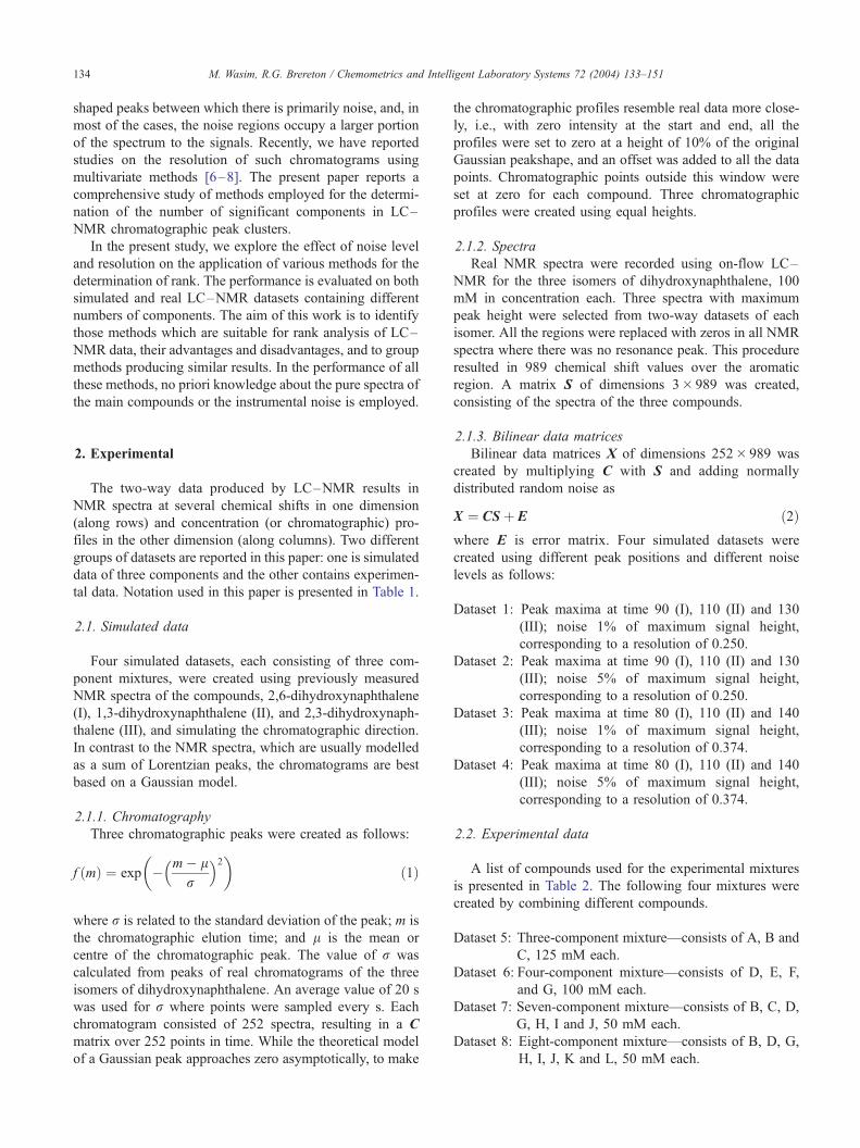
it determined the correct rank. Fig. 1 is a plot of the

logarithm of eigenvalues for dataset 5 where there is no

indication about the data rank. For the same dataset, the

results of the eigenvalue ratio method are produced in Fig.

2. The results for these three methods have been compiled in

Table 4.

4.2. Error indicator functions (INF)

It has been explained in Section 3.2.2 that the rank was

determined by plotting error indicator functions against the

number of components and then locating a break in the

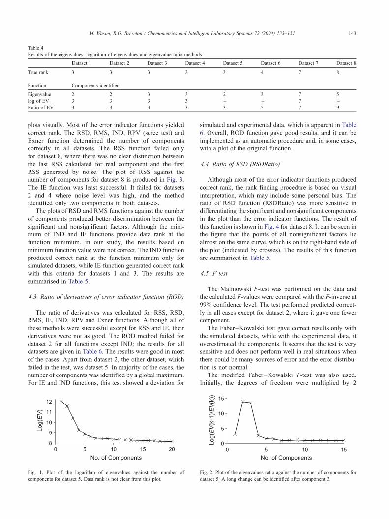
Table 4

Results of the eigenvalues, logarithm of eigenvalues and eigenvalue ratio methods

Dataset 1 Dataset 2 Dataset 3 Dataset 4 Dataset 5 Dataset 6 Dataset 7 Dataset 8

True rank 3 3 3 3 3 4 7 8

Function Components identified

Eigenvalue 2 2 3 3 2 3 7 5

log of EV 3 3 3 3 – – 7 –

Ratio of EV 3 3 3 3 3 5 7 9


plots visually. Most of the error indicator functions yielded

correct rank. The RSD, RMS, IND, RPV (scree test) and

Exner function determined the number of components

correctly in all datasets. The RSS function failed only

for dataset 8, where there was no clear distinction between

the last RSS calculated for real component and the first

RSS generated by noise. The plot of RSS against the

number of components for dataset 8 is produced in Fig. 3.

The IE function was least successful. It failed for datasets

2 and 4 where noise level was high, and the method

identified only two components in both datasets.

The plots of RSD and RMS functions against the number

of components produced better discrimination between the

significant and nonsignificant factors. Although the mini-

mum of IND and IE functions provide data rank at the

function minimum, in our study, the results based on

minimum function value were not correct. The IND function

produced correct rank at the function minimum only for

simulated datasets, while IE function generated correct rank

with this criteria for datasets 1 and 3. The results are

summarised in Table 5.

4.3. Ratio of derivatives of error indicator function (ROD)

The ratio of derivatives was calculated for RSS, RSD,

RMS, IE, IND, RPV and Exner functions. Although all of

these methods were successful except for RSS and IE, their

derivatives were not as good. The ROD method failed for

dataset 2 for all functions except IND; the results for all

datasets are given in Table 6. The results were good in most

of the cases. Apart from dataset 2, the other dataset, which

failed in the test, was dataset 5. In majority of the cases, the

number of components was identified by a global maximum.

For IE and IND functions, this test showed a deviation for

Fig. 1. Plot of the logarithm of eigenvalues against the number of

components for dataset 5. Data rank is not clear from this plot.

simulated and experimental data, which is apparent in Table

6. Overall, ROD function gave good results, and it can be

implemented as an automatic procedure and, in some cases,

with a plot of the original function.

4.4. Ratio of RSD (RSDRatio)

Although most of the error indicator functions produced

correct rank, the rank finding procedure is based on visual

interpretation, which may include some personal bias. The

ratio of RSD function (RSDRatio) was more sensitive in

differentiating the significant and nonsignificant components

in the plot than the error indicator functions. The result of

this function is shown in Fig. 4 for dataset 8. It can be seen in

the figure that the points of all nonsignificant factors lie

almost on the same curve, which is on the right-hand side of

the plot (indicated by crosses). The results of this function

are summarised in Table 5.

4.5. F-test

The Malinowski F-test was performed on the data and

the calculated F-values were compared with the F-inverse at

99% confidence level. The test performed predicted correct-

ly in all cases except for dataset 2, where it gave one fewer

component.

The Faber–Kowalski test gave correct results only with

the simulated datasets, while with the experimental data, it

overestimated the components. It seems that the test is very

sensitive and does not perform well in real situations when

there could be many sources of error and the error distribu-

tion is not normal.

The modified Faber–Kowalski F-test was also used.

Initially, the degrees of freedom were multiplied by 2

Fig. 2. Plot of the eigenvalues ratio against the number of components for

dataset 5. A long change can be identified after component 3.

Fig. 3. RSS plot of dataset 8 (real dataset). The data rank is not clear in the

plot.

Fig. 4. RSD(K)/RSD(K� 1) ratio of dataset 8 (real dataset). Significant

factors are indicated by w .

M. Wasim, R.G. Brereton / Chemometrics and Intell144

[h = 2 in Eq. (21)] and later with 10; in both cases, the

results were not correct (Table 7).

4.6. Cross-validation

As with other methods, cross-validation can also be

applied first by the inspection of plots, and then by

comparison based on PRESS and RSS values. Visual

inspection of all PRESS and RSS plots show true number

of components except in dataset 8, but the results based on

the ratio of PRESS and RSS gave the correct number of

components only in the case of simulated datasets and

predicted too many significant components in the experi-

mental datasets. Therefore, cross-validation based on the

visual inspection of PRESS and RSS plots leads to better

results.

4.7. Morphological score (MS)

The morphological score was, initially, applied to the

spectra obtained by OPA; the results were not correct

because OPA dissimilarity plots did not give true number

of components. It was also applied to the whole dataset,

which excluded the OPA calculations. The results showed

that the method worked only for simulated data, although it

provided good results when the number of components was

estimated by visual inspection of the plot of morphological

score against number of components, as shown in Figs. 5

and 6. Dataset 5 gave a correct result; the plot of dataset 6

showed the last two points, corresponding to real compo-

nents, slightly above the MS values of noise. Dataset 7 gave

six components, the first five MS values were well above

MS of noise but the sixth MS was below the noise level.

The seventh MS was higher than the noise level, thus

estimating six components in total.

4.8. Orthogonal projection approach (OPA)

OPAwas applied on object (time) and variable (chemical

shift) dimensions. As discussed in Section 3.2.8, OPA

produces dissimilarity plots, which can be utilised in differ-

ent ways to identify the number of components. We discuss

the results of these methods in Sections 4.8.1–4.8.3.

4.8.1. Dissimilarity plots

4.8.1.1. Object selection. All the simulated datasets pro-

vided correct results except dataset 1, which showed one

more component. In real datasets, only datasets 5 and 6

produced the correct results while datasets 7 and 8 gave

higher components.

4.8.1.2. Variable selection. All the simulated datasets

produced correct results except for dataset 2, in which

one less component was predicted than the true rank. In

all the real datasets, the number of significant components

was overestimated. Most of the results using dissimilarity

plots, on the time dimension, were not correct. Using the

variable dimension, the results were totally wrong be-

cause, in majority of cases, more components than

expected were found due to the reasons explained in

Section 3.2.9.3.

4.8.2. Durbin–Watson statistics (dw)

4.8.2.1. dw on object selection. The dw statistics produced

correct results only with datasets 1 and 3, which are

simulations. It found two components in datasets 2 and 4,

which contained high-noise levels. There was no clear

indication about the number of components in experimental

datasets. Figs. 7 and 8 show the dw plots for dataset 8 using

OPA data on two different dimensions.

4.8.2.2. dw on variable selection. The results calculated

by Durbin–Watson statistics were plotted and the number

of components calculated by determining where there was a

sharp increase in value. In most of the cases, less compo-

nents were found than the true rank. The success of the dw

test was high when it was used with dissimilarity values

obtained using variable dimension. It was successful in

most of the cases, as shown in Table 7. There was no

difference in simulated or real datasets from the success

point of view.

4.8.3. Concentration profiles

Concentration plots provided good results in all cases. As

OPA does not yield pure variables, therefore, some profiles

igent Laboratory Systems 72 (2004) 133–151

Table 5

Results of error indicator functions and RSD ratio compiled together


True rank 3 3 3 3 3 4 7 8


RSS 3 3 3 3 3 4 7 7–8

RSD 3 3 3 3 3 4 7 8

RMS 3 3 3 3 3 4 7 8

IE 3 2 3 2 3 4 7 8

IND 3 3 3 3 3 4 7 8

RPV 3 3 3 3 3 4 7 8

w 3 3 3 3 3 4 7 8

RSDRatio 3 3 3 3 3 4 7 8


appear which extend over two or more than two compo-

nents. Fig. 9 shows concentration profiles of dataset 1. The

profiles for chemical shift, d, of 7.112 and 7.109 ppm

belong to the fastest eluting compound, and similarly those

for 6.722 and 6.726 ppm belong to the second eluting

compound. The profile for 7.196 ppm arises from the

slowest eluting compound, while the concentration plot

obtained by using 7.252 ppm starts with the middle eluting

compound and ends with the slowest eluting compound,

which can easily be identified as a combined profile that

originates from two close resonances (variables) from the

middle and slowest eluting compounds together. After

excluding the mixed profile, the presence of three compo-

nents is confirmed in dataset 1. Datasets 2 and 3 also show

similar profiles but at different chemical shifts. Dataset 4

does not show any common resonance, and the concentra-

tion plots are very clean for the three compounds.

In dataset 5, three components were correctly identified.

For dataset 6, initially, six concentration profiles were

generated. The second variable (7.112 ppm) is not a pure

variable and its concentration profile is indicative of two

components; it was not difficult to correctly identify the

true number of components. Dataset 7 resulted in interest-

ing plots; the first variable selected by OPA at 1.337 ppm

is not a pure variable and it belonged to compounds eluting

as sixth and seventh components in concentration plots

(see Fig. 10 which shows the first nine concentration

Fig. 5. Morphological score (MS) on dataset 1 (three components). Three

components can be easily discriminated (see horizontal line).

profiles). After deleting the first concentration profile

(which corresponds to a combination of the sixth and

seventh eluting compounds) and the last profile (which is

the same as the third component), it suggests that there is a

total of seven components in the mixture. Dataset 8 also

exhibited similar behaviour, and it also showed some

variables that correspond to a combination of two pure

components, but these were identified and the true dimen-

sionality of the data was determined correctly. Thus, using

the concentration profiles followed by OPA was a success-

ful approach in finding the true rank of the data in

simulated as well as in real datasets.

4.9. SIMPLISMA

SIMPLISMA is very sensitive to noise if the noise level

is high as it often selects components from noise. The effect

of noise could be reduced either by reducing the objects

dimension or by increasing the offset value. The latter

procedure is not recommended because, in that case, SIM-

PLISMAwill generate variables similar to OPA. The former

procedure was adopted, and chromatographic profiles were

discarded at the start and at the end of all datasets. It

significantly improved the results. SIMPLISMAwas applied

at an offset value of 15% on both dimensions.

Fig. 6. Morphological score (MS) on dataset 8 (eight components).

Discrimination is not good; only seven components can be found (see

horizontal line).

Fig. 7. Durbin –Watson statistics calculated on dissimilarity values

calculated by OPA on variable dimension using dataset 8 (eight

components).

Fig. 9. Concentration plots of the first six variables selected by OPA using

dataset 1 (simulated data).


Like OPA, SIMPLISMA also makes use of several

methods in determining the data rank; in our study we used

four such methods. The results with these methods are

discussed in the Sections 4.9.1–4.9.4.

4.9.1. Purity plots

4.9.1.1. Object selection. Datasets 1, 3, 5 and 6 gave the

true rank, while datasets 2 and 4 gave one component less

than the true rank. Datasets 7 and 8 did not provide any

conclusive answers because the purity plots became very

complex after six components were detected, and so it was

difficult to decide the real number of components.

4.9.1.2. Variable selection. From datasets 1 and 3, three

components were predicted, and from datasets 2 and 4, two

components were predicted. Datasets 5 and 6 produced the

true rank. It was difficult to find out the true number of

components in datasets 7 and 8, where more components

appeared than the true rank.

Purity plots behaved in a similar manner to OPA dissim-

ilarity plots; that is, both of the methods yielded incorrect

rank in the majority of datasets. Like OPA, purity plots also

failed in the case of simulated datasets.

4.9.2. Residual sum of squares using SIMPLISMA

4.9.2.1. Object selection. Datasets 1, 3, 5 and 6 gave the

correct results. The remainder predicted a lower rank than

Fig. 8. Durbin –Watson statistics calculated on dissimilarity values

calculated by OPA on time dimension using dataset 8 (eight components).

the true one. These results suggest that rssq provides good

results in most of cases. In our present study, rssq plots

based on the variable selection gave better results than the

plots based on object dimension.

4.9.2.2. Variable selection. The rssq gave wrong results

for dataset 2, and dataset 6 did not produce good evidence

for the three components; there was some indication of

the existence of a fourth component. Similarly for dataset

8, either seven or nine components are suggested; there

was a slight decrease in the rssq value when the ninth

component was selected. The rssq plot of dataset 8 can be

seen in Fig. 11.

4.9.3. Durbin–Watson statistics (dw)

4.9.3.1. Object selection. Durbin–Watson gave correct

results only in dataset 3, and, in the rest of datasets, the

results were incorrect.

Fig. 10. Concentration plots of the first nine variables selected by OPA

using dataset 7 (real data).

Fig. 11. Residual sum of square (rssq) calculated by SIMPLISMA on the

time dimension using dataset 8 (eight components).

Fig. 13. Concentration plots of the first five variables selected by

SIMPLISMA using dataset 5 (real data).


4.9.3.2. Variable selection. Durbin–Watson was totally

unable to provide answer about the number of components.

The plots were without minima and did not show any rise

after the true number of components.

4.9.4. Concentration profiles

When OPA and SIMPLISMA are applied to the variable

dimension, in most cases, they found more components than

the true number, as estimated by dissimilarity or purity

plots. In Section 4.8.3, it was discussed that concentration

profiles proved successful in OPA. The concentration pro-

files become complicated when the number of components

becomes large and requires a careful inspection of plots.

Fig. 12 shows the concentration plots of the first four

variables of dataset 1 obtained by SIMPLISMA. It is easy

to identify that the fourth component is the same as the

third component. Furthermore, this can be confirmed by

calculating the correlation coefficient between profiles 3

and 4, which is greater than 0.9, suggesting that both

profiles are very similar. Concentration profiles obtained

by SIMPLISMA on the time dimension gave correct

results in all cases except dataset 5 where it suggested

four components as shown in Fig. 13. It can be seen that

the fourth component is approximately similar to the third

Fig. 12. Concentration plots of the first four variables selected by

SIMPLISMA using dataset 1 (simulated data).

component but, due to the high level of noise present in

these profiles, it is not very clear, and the fifth component

is the same as the first component. Concentration profiles

of dataset 7 are given in Fig. 14. Among these profiles, the

profiles obtained using chemical shift d at 7.177 and 7.182

ppm belong to the same component; the profiles from the

chemical shifts at 2.450 and 2.464 ppm are also from a

single compound, while the profile at 1.323 ppm is a

combined profile of components 6 and 7. On deleting

these profiles, seven components remain, which is a

correct number for this dataset. Similarly, 8 components

are identified in dataset 8. Fig. 15 shows the concentration

profiles for dataset 8.

As concentration profiles selected by SIMPLISMA have

more noise than those selected by OPA, it makes the

identification process more difficult, and, sometimes, an

incorrect number of components is identified as in the case

of dataset 5.

Fig. 14. Concentration plots of the first ten variables selected by


Fig. 15. Concentration plots of the first eleven variables selected by


Fig. 16. EPCIA on dataset 6 (four components) fourth plot showing a peak-

like structure.

Fig. 17. EPCIA on dataset 6 (four components) after using five variables.


4.10. Correlation plots

In our present study, correlation plots did not provide a

suitable approach in finding the true number of components,

and were successful only in one case, which was dataset 6.

It gave one component less than the true rank in the

simulated datasets and datasets 5 and 7. In dataset 8, this

method finds two components less than the true rank.

Therefore, it suggests that this technique is not very sensi-

tive and underestimates the true number of components.

Correlation plots work well when chromatographic resolu-

tion is high, although the data-preprocessing step removes

most of the noise but not completely. Noise is removed from

those frequencies where there appears no peak from all the

components under investigation.

4.11. Derivative plots

In the same way as correlation plots, derivatives yielded

incorrect results. Datasets 1, 3, 4 and 5 produced one

component less, and dataset 2 showed two components less

than the true rank. The derivatives in the present study were

successful only in the case of dataset 6. The method found

six components in datasets 7 and seven components in

dataset 8. The presence of noise and low resolution appears

to be the possible reason for the failure of the method.

4.12. Evolving principal component analysis (EPCA)

EPCA–EW was another successful method. This method

was not only successful in all cases but this method was the

easiest in interpretation of its plots. The results were correct

in all cases. The method of FSW–EFA was successful only

in two cases, datasets 6 and 7. In all other cases, it produced

one component less than the true rank, even with the

simulated datasets. This method did not perform well in

one of our previous study [5] of a three-component mixture,

which could be due to a high level of noise.

4.13. Evolving principal component innovation analysis

(EPCIA)

In EPCIA, the number of components can be found by

looking at the RMS plots, their shape and the changes in the

RMS plots after selecting different numbers of components.

In our study, we used OPA and SIMPLISMA data as an

input to EPCIA. Datasets 1, 3 and 4 gave similar OPA and

SIMPLISMA variables. Therefore, the results of EPCIA

were same and correct for these samples. We discuss results

of other datasets in Sections 4.13.1 and 4.13.2.

4.13.1. OPA selected variables

Dataset 2 suggests four significant components, and, in

dataset 5, there were three significant components. There

was a small peak in the third plot of dataset 5, which could

be assigned to a fourth component but this peak persisted

even after the addition of fourth profile. Therefore, this

method suggests that dataset 5 contains only three compo-

nents. Dataset 6 showed four components by both methods

(OPA and SIMPLISMA). It also behaved similarly to data-

set 5 and the last plot did not show complete randomness as

shown in Figs. 16 and 17. For dataset 7, 10 OPA variables

were used as input; among those, four appeared to have

small impact on the reduction of RMS values. If those

variables were regarded as impure or insignificant, this

suggests that dataset 7 consists of six significant compo-

Fig. 18. Subspace discrepancy function D(K) (diamonds) and sin2(#K)

(stars) for PCA scores and OPA variables using dataset 2.


nents. A similar observation was made for dataset 8,

yielding seven components when 10 OPA variables were

modelled.

4.13.2. SIMPLISMA selected variables

Datasets 2, 5 and 6 gave correct results. EPCIA proved to

be difficult when the number of components becomes large.

It has been found that, in the analysis, some specific

variables behave less effectively. One such variable can be

located in dataset 7, which is the fourth variable. If this is

removed and EPCIA is performed again with six variables,

the results are almost the same when seven components

were modelled. Thus, in this case, it can be concluded that

there are six true components in this mixture. Dataset

8 produces randomness in the RMS plot after eight variables

have been used. Again in this case, the fourth variable has

very low influence on the overall reduction of the RMS

value or the shape of RMS plot. If this is removed and

EPCIA is performed again with seven variables, the results

are the same. These observations lead to a conclusion that

some variables, which show a small change in the reduction

of RMS values, appear to be less effective and cannot be

taken as a new component. Finally, a small peak-like

structure was seen in the last RMS plot of all experimental

datasets, which indicates that either the variables are not

pure or the variables are not sufficient to model the data.

Table 6

Results of ROD on different error indicator functions

Components identified

Dataset 1 Dataset 2 Dataset 3 Dataset

True rank 3 3 3 3


RSS 3 2 3 3

RSD 3 2 3 3

RMS 3 2 3 3

IE 3a 2b 3a 2b

IND 3b 3b 3b 3b

RPV 3 2 3 3

w 3 2 3 3

a First minimum in ROD plot and function minimum.b Global minimum in ROD plot and function minimum.

4.14. Subspace comparison

Subspace comparison produced promising results. PCA

scores and variables from OPA and SIMPLISMAwere used

as input for this test. The three methods produced three

combinations of variables, namely, PCA scores and SIM-

PLISMA variables, PCA scores and OPA variables, and

SIMPLISMA variables and OPA variables. It is difficult to

correctly interpret the results from the description given in

reference [50] because the criterion is a qualitative one.

Neither of the combinations could identify the correct

number of components in dataset 2; there is some indication

about the third component in the subspace discrepancy plot

using scores from PCA scores and OPA variables, as shown

in Fig. 18. A similar situation existed in other cases; for

example, dataset 6 appears to consist of either three or four

components (the third component has lower value than the

fourth component) using variables from SIMPLISMA and

OPA. Best results and better discrimination were obtained

using PCA scores and OPA variables, and PCA scores and

SIMPLISMA variables. Subspace comparison, although

relying on other methods for variable selection, is simple

to implement and fast to use.

5. Summary of results

All of the methods have been compiled in Tables 4–7.

Five methods could be selected as the best for providing true

rank. The first is a set of error indicator functions (RSD,

RMS, IND, RPVand Exner function), second is ROD on IND

function, third is RSD ratio, fourth is concentration plots

using OPA, and the last method is EPCA–EW. However, all

of these methods rely on visual interpretation of various plots,

except ROD on IND function. As the visual interpretation of

plots may vary from person to person, therefore, the final

results may be prone to some bias and are hard to automate.

Dataset 2 has the highest level of noise and lowest resolution.

4 Dataset 5 Dataset 6 Dataset 7 Dataset 8

3 4 7 8

2 4 7 8

3 4 7 8

3 4 7 8

3b 4 7 8

3 4 7 8

2 4 7 8

3 4 7 8

Table 7

Results of all methods except eigenvalue based methods


True components 3 3 3 3 3 4 7 8

Indicator Components identified

Malinowski’s F-test (a= 0.01) 3 2 3 3 3 4 7 8

Faber–Kowalski F-test 3 3 3 3 >3 >4 >7 >8

Modified FK F-test (h= 2) 3 3 3 3 >3 >4 >7 >8

Modified FK F-test (h= 10) 3 2 3 3 3 4 8 11

Morphological score 3 3 3 3 3 4 6 7

Cross-validation 3 3 3 3 6 5 8 10

OPA

Dissimilarity plots (time dim.) 4 3 3 3 4 4 9 10

Dissimilarity plots (var. dim.) 3 2 3 3 4 5 >7 >8

Durbin–Watson (time dim.) 3 2 3 2 3 2 – –

Durbin–Watson (var. dim.) 3 3 4 3 2 4 7 8

Concentration profiles 3 3 3 3 3 4 7 8

SIMPLISMA

Purity plots (time dim.) 3 2 3 2 3 4 9 >8

Purity plots (var. dim.) 3 2 3 2 3 4 7–8 >8

Durbin–Watson (time dim.) – – 3 – 2 2 7 10

Durbin–Watson (var. dim.) – – – – 2 3 7 6

RSS (time dim.) 3 2 3 2 3 4 6 6

RSS (var. dim.) 3 2 3 3 3 3 or 4 7 6

Concentration profiles 3 3 3 3 4 4 7 8

Correlation plot 2 2 2 2 2 4 6 6

Derivative plot 2 1 2 1 or 2 2 4 6–7 6

EPCA

Expanding window 3 3 3 3 3 4 7 8

Fixed size moving window 2 2 2 2 2 4 7 8

EPCIA

OPA variables 3 4 3 3 3 4 6 7

SIMPLISMA variables 3 3 3 3 3 4 6 7

Subspace comparison

SIMPLISMA and OPA 3 2 3 2 3 3 7 8

PCA scores and SIMPLISMA 3 2 3 3 3 4 7 8

PCA scores and OPA 3 2 3 3 3 4 7 8


If the results of this dataset are omitted, then RSS, Malinow-

ski’s F-test, concentration profiles using SIMPLISMA and

subspace comparison with PCA score perform well. The

methods that least often predicted the correct rank were

Durbin–Watson statistics on SIMPLISMA variables, corre-

lation plots and derivative plots. The rank estimation in

dataset 3 was correctly determined by most of the methods;

this was primarily due to good resolution and a well-defined

noise distribution in the data. The relative effectiveness of

methods for LC–NMR data differ quite strongly to LC–

DAD because there are different characteristics in the spectra.

In NMR, there are often quite distinct and well-defined

spectral peaks, whereas in uv/vis spectroscopy, the spectral

peaks tend to be much broader and less well defined. In

addition, the noise levels in NMR are often much higher than

in uv/vis. In LC–NMR, it is not easy to eliminate noise by

preprocessing because there are always regions where there

are resonances in the spectrum of one compound and noise in

the spectrum of another, so that noise regions will be retained

even after variable selection. In addition, there can be slight

drifts in peak positions in LC–NMR peak positions during

recording which, because of the relatively sharp nature of

these peaks, has an influence on the effectiveness of certain

methods; this problem is not usually encountered in LC–

DAD. Hence, methods such as correlation coefficients and

derivatives that are very effective in LC–DAD because of the

smooth and relatively noise-free nature of the data are less

useful in LC–NMR which technique is a challenge for the

chemometrician.

Automation is a desirable feature for any algorithm.

Only two of the successful methods can readily be

automated, one is Malinowski’s F-test and the other is

ROD on IND function. The ROD was successful for all

datasets using IND function, while Malinowski’s F-test

failed for dataset 2 which had high noise and low

resolution.


As artefacts make it difficult to identify correct data rank,

all those methods which depend on eigenvalues, are strongly

influenced by the existence of artefacts. Moreover, the

interpretation becomes difficult when the noise level is high.

Successful methods, which do not rely on eigenvalues, are

OPA dissimilarity plots, SIMPLISMA purity plots and

concentration plots. Among these methods, concentration

plots using OPA variables was the most successful.

Most of the methods estimated less components than the

true rank except log of eigenvalues, eigenvalues ratio, FK F-

test, modified FK test, cross-validation, OPA and SIM-

PLISMA and subspace comparison (only by SIMPLISMA

and OPA data), which gave more components.

Acknowledgements

M.W. wishes to thank the Ministry of Science and

Technology, Government of Pakistan for their funding and

the support of PAEC, Pakistan. We thank Drs. C. Airiau and

M. Murray for help with the experimental work.

References

[1] F.C. Sanchez, B.V.D. Bogaert, S.C. Rutan, D.L. Massart, Chemom.

Intell. Lab. Syst. 34 (1996) 139–171.

[2] E.R. Malinowski, Factor Analysis in Chemistry, third ed., Wiley, New

York, 1991.

[3] M. Meloun, J. Capek, P. Miksik, R.G. Brereton, Anal. Chim. Acta

423 (2000) 51–68.

[4] J. Toft, Chemom. Intell. Lab. Syst. 29 (1995) 189–212.

[5] M. Wasim, M.S. Hassan, R.G. Brereton, Analyst 128 (2003)

1082–1090.

[6] H. Shen, C.Y. Airiau, R.G. Brereton, Chemom. Intell. Lab. Syst. 62

(2002) 61–78.

[7] H. Shen, C.Y. Airiau, R.G. Brereton, J. Chemom. 16 (2002) 165–175.

[8] H. Shen, C.Y. Airiau, R.G. Brereton, J. Chemom. 16 (2002) 469–481.

[9] J.C. Hoch, A.S. Stern, NMR Data Processing, Wiley-Liss, New York,

1996.

[10] S. Wold, K. Esbensen, P. Geladi, Chemom. Intell. Lab. Syst. 2 (1987)

37–52.

[11] H. Wold, in: J. Gani (Ed.), Soft Modelling by Latent Variables: the

Nonlinear Iterative Partial Least Squares (NIPALS) Algorithm, Per-

spectives in Probability and Statistics, Academic Press, London,

1975, pp. 117–142.

[12] T.M. Rossi, I.M. Warner, Anal. Chem. 54 (1986) 810–815.

[13] N. Ohta, Anal. Chem. 45 (1973) 553–557.

[14] I.T. Jollife, Principal Component Analysis, Springer, New York, 1986.

[15] R.F. Hirsch, G.L. Wu, Chemom. Intell. Lab. Syst. 1 (1987) 265–272.

[16] R.G. Brereton, Chemometrics: Data Analysis for the Laboratory and

Chemical Plant, Wiley, Chichester, 2003.

[17] E.R. Malinowski, Anal. Chem. 49 (1977) 612–617.

[18] R.B. Cattell, Multivariate Behav. Res. 1 (1966) 245–276.

[19] H.H. Kindsvater, P.H. Weiner, T.J. Klingen, Anal. Chem. 46 (1974)

982–988.

[20] O. Exner, Collection of Czech, Chem. Commun. 31 (1966)

3222–3251.

[21] A. Elbergali, J. Nygren, M. Kubista, Anal. Chim. Acta 379 (1999)

143–158.

[22] E.R. Malinowski, J. Chemom. 3 (1988) 49–60.

[23] E.R. Malinowski, J. Chemom. 4 (1990) 102.

[24] K. Faber, B.R. Kowalski, Anal. Chim. Acta 337 (1997) 57–71.

[25] N.K.M. Faber, Comput. Chem. 23 (1999) 565–570.

[26] J. Mandel, Technometrics 13 (1971) 1–18.

[27] E.R. Malinowski, J. Chemom. 13 (1999) 69–81.

[28] S. Wold, Technometrics 20 (1978) 397–405.

[29] D.W. Osten, J. Chemom. 2 (1988) 39–48.

[30] H. Shen, L. Stordrange, R. Manne, O.M. Kvalheim, Y. Liang, Che-

mom. Intell. Lab. Syst. 50 (2000) 37–47.

[31] F.C. Sanchez, J. Toft, B. Van den Bogaert, D.L. Massart, Anal. Chem.

68 (1996) 79–85.

[32] W. Windig, C.E. Heckler, F.A. Agblevor, R.J. Evans, Chemom. Intell.

Lab. Syst. 14 (1992) 195–207.

[33] N.R. Draper, H. Smith, Applied Regression Analysis, third ed., Wiley,

New York, 1998.

[34] S. Gourvenec, D.L. Massart, D.N. Rutledge, Chemom. Intell. Lab.

Syst. 61 (2002) 51–61.

[35] G. Strang, Linear Algebra and its Applications, third ed., Harcourt

Brace Jovanovich, Orlando, 1998.

[36] A. Savitzky, M.J.E. Golay, Anal. Chem. 36 (1964) 1627–1639.

[37] J. Steinier, Anal. Chem. 44 (1972) 1906–1909.

[38] K. Kavianpour, R.G. Brereton, Analyst 123 (1998) 2035–2042.

[39] S. Dunkerley, R.G. Brereton, J. Crosby, Chemom. Intell. Lab. Syst. 48

(1999) 99–119.

[40] M. Maeder, Anal. Chem. 59 (1987) 527–530.

[41] B.G.M. Vandeginste, D.L. Massart, L.M.C. Buydens, S. De Jong, P.J.

Lewi, J. Smeyers-Verbeke, Handbook of Chemometrics and Quali-

metrics, Part B, Elsevier, Amsterdam, 1998, pp. 274–278.

[42] H.R. Keller, D.L. Massart, Anal. Chim. Acta 246 (1991) 379–390.

[43] H.R. Keller, D.L. Massart, J.O. De Beer, Anal. Chem. 65 (1993)

471–475.

[44] J. Toft, O.M. Kvalheim, Chemom. Intell. Lab. Syst. 19 (1993) 65–73.

[45] F. Cuesta Sanchez, J. Toft, O.M. Kvalheim, D.L. Massart, Anal.

Chim. Acta 314 (1995) 131–139.

[46] S.C. Rutan, J. Chemom. 1 (1987) 7–18.

[47] G.H. Webster, T.L. Cecil, S.C. Rutan, J. Chemom. 3 (1988) 21–32.

[48] S.J. Vanslyke, P.D. Wentzell, Anal. Chem. 63 (1991) 2512–2519.

[49] P.D. Wentzell, S.G. Hughes, S.J. Vanslyke, Anal. Chim. Acta 307

(1995) 459–470.

[50] H. Shen, Y. Liang, O.M. Kvalheim, R. Manne, Chemom. Intell. Lab.

Syst. 51 (2000) 49–59.

determination of the number of significant components in liquid chromatography nuclear magnetic...

Documents