determination of sub-photosphere solar active …
TRANSCRIPT

DETERMINATION OF SUB-PHOTOSPHERE SOLAR ACTIVE REGION 3D MAGNETIC FIELD STRUCTURE FROM EMERGENCE OBSERVATIONS
Committee:
Date:
by
Brian Briggs A Thesis
Submitted to the Graduate Faculty
of George Mason University in Partial Fulfillment of
The Requirements for the Degree of
Master of Science Applied and Engineering Physics
Dr. Jie Zhang, Thesis Director
Dr. Robert Weigel, Committee Member
Dr. Joeseph Weingartner, Committee Member
Dr. Michael Summers, Department Chairperson
Dr. Timothy L. Born, Associate Dean for Student and Academic Affairs, College of Science
Dr. Vikas Chandhoke, Dean, College of Science
Fall Semester 2012 George Mason University Fairfax, VA

Determination of Sub-Photosphere Solar Active Region 3D Magnetic Field Structure from
Emergence Observations
A thesis submitted in partial fulfillment of the requirements for the degree of Master of Science at George Mason University
By
Brian S. Briggs Bachelor of Science
University of Central Florida, 2002
Director: Jie Zhang, Associate Professor School of Physics, Astronomy, and Computational Sciences
Fall Semester 2012 George Mason University
Fairfax, VA

ii
ACKNOWLEDGEMENTS
I would like to thank the Jie Zhang, Ph.D. for his guidance and support throughout the research effort put forth in this thesis. Also, I would like to thank George Chintzoglou for his assistance with learning IDL and sharing the techniques for data processing and visualization used in this thesis. Finally, I would like to thank Orbital Sciences Corporation for their financial support and flexibility throughout my graduate studies.

iii
TABLE OF CONTENTS
Page
LIST OF TABLES ........................................................................................................................ iv
LIST OF FIGURES ....................................................................................................................... v
ABSTRACT .................................................................................................................................. vii
CHAPTER 1: INTRODUCTION ................................................................................................. 1
OVERVIEW OF SOLAR ACTIVE REGIONS ........................................................................................ 1 OVERVIEW OF SOLAR ACTIVE REGIONS AND MAGNETIC FLUX EMERGENCE ................................ 4 STATEMENT OF WORK .................................................................................................................. 7
CHAPTER 2: DATA, OBSERVATIONS, AND PROCESSING .............................................. 9
SDO MISSION / HMI INSTRUMENT ............................................................................................... 9 ACTIVE REGION SELECTION ........................................................................................................ 13 DATA SET SELECTION ................................................................................................................. 19 DATA PROCESSING ..................................................................................................................... 21 3D VISUALIZATION .................................................................................................................... 26
CHAPTER 3: RESULTS ............................................................................................................ 32
OBSERVATIONAL DATA AND MODELING ................................................................................... 32 3D VISUALIZATION OF MODELED ACTIVE REGION ................................................................... 43 EMERGENCE ANGLES AND HEIGHTS .......................................................................................... 45
CHAPTER 4: INTERPRETATION OF RESULTS ................................................................. 50
COMPARISON TO PREVIOUS OBSERVATION-BASED WORK ......................................................... 50 COMPARISON OF RESULTS TO EXISTING FLUX EMERGENCE MODELS ......................................... 52
CHAPTER 5: SUMMARY ......................................................................................................... 66
REFERENCES ............................................................................................................................. 69

iv
LIST OF TABLES
Page
Table 1 – Polarity tilt angles vs. flux tube rise velocity ................................................................. 49
Table 2 – AR flux and geometric parameters summary ................................................................ 67

v
LIST OF FIGURES
Page
Figure 1 - Sunspot groups as viewed in the visible spectrum (image credit: NASA/Solar
Dynamics Observatory) ................................................................................................................... 1
Figure 2 – Solar coronal loops (image credit: NASA/Solar Dynamics Observatory) ..................... 2
Figure 3 – Flare and coronal mass ejection (image credit: NASA/Solar Dynamics Observatory) .. 3
Figure 4 – Aurora viewed from the International Space Station (image credit: NASA/ISS
Expedition 23) .................................................................................................................................. 4
Figure 5 – Flux tube evolution (D’silva & Choudhuri 1993) .......................................................... 5
Figure 6 – Mean observed AR tilt angles (y-axis) vs. latitude (x-axis) (Hale, et al. 1919) ............. 6
Figure 7 – Emergence of flux into the corona (Zwaan 1985) .......................................................... 7
Figure 8 – SDO spacecraft (Pesnell, et al. 2012) ........................................................................... 10
Figure 9 – AIA (171 Å) and HMI (magnetogram) imagery (image credit: NASA/Solar Dynamics
Observatory) .................................................................................................................................. 11
Figure 10 – HMI instrument (HMI Team 2012) ............................................................................ 12
Figure 11 – HMI Optical layout (Schou, et al. 2012) .................................................................... 13
Figure 12 – Candidate AR 11149 .................................................................................................. 14
Figure 13 – Candidate AR (not numbered) .................................................................................... 15
Figure 14 – Candidate AR 11184 .................................................................................................. 16
Figure 15 – Candidate AR 11250 .................................................................................................. 16
Figure 16 – Candidate AR 11282 .................................................................................................. 17
Figure 17 – Candidate AR 11311 .................................................................................................. 18
Figure 18 – Candidate AR 11318 .................................................................................................. 18
Figure 19 – Candidate AR 11416 .................................................................................................. 19
Figure 20 – AR 11416 evolution with polarity peaks (x symbols) and centroids (+ symbols)
overlaid .......................................................................................................................................... 20
Figure 21 – Magnetogram prior to (left) and after (right) derotation ............................................ 21
Figure 22– Derotated and cropped reference image ...................................................................... 22
Figure 23 – AIA 4500 imagery of AR 11416 ................................................................................ 24

vi
Figure 24 – Quiet sun histogram: (a) full scale, (b) zoomed to max=20 ....................................... 25
Figure 25 – 3D visualization of datacube ...................................................................................... 27
Figure 26 – Image slices as datacube inputs .................................................................................. 28
Figure 27 – Datacube viewed from +Y (left) and –Y (right) ......................................................... 29
Figure 28 – Datacube viewed from +Z .......................................................................................... 30
Figure 29 – Datacube with polarity peak values (left) and center/centroid (right) traces inlaid .... 30
Figure 30 – Line-of-sight magnetic flux by polarity versus time .................................................. 32
Figure 31 – Polarity separation versus time ................................................................................... 34
Figure 32 – Polarity separation speed versus time ......................................................................... 36
Figure 33 – Tilt and radius of bipolar AR with flux peaks (x symbols) and flux centroids (+
symbols) overlaid ........................................................................................................................... 37
Figure 34 – Tilt angle evolution ..................................................................................................... 38
Figure 35 – Center motion versus time .......................................................................................... 39
Figure 36 – Apparent motion of center relative to centroids ......................................................... 42
Figure 37 – Apparent motion of centroids (“_bar” entries) versus peak fluxes ............................. 43
Figure 38 – Quality of fit for center and centroids (green lines) ................................................... 44
Figure 39 – Polarity radius vs. distance for v=0.1 km/s ................................................................ 46
Figure 40 – 3D contour plot and centroid trace of flux tube with displacement on z axis (0.1km/s
rise rate assumed) ........................................................................................................................... 46
Figure 41 – 3D contour plot and centroid trace of flux tube with displacement on z axis (0.1km/s
rise rate assumed) ........................................................................................................................... 47
Figure 42 – Angle of flux emergence (centroids) .......................................................................... 48
Figure 43 – Flux rope shape and evolution of McMath 13043 (Tanaka 1991) ............................. 51
Figure 44 – Proper motion of polarity tracks and inferred 3D structure (Leka, et al. 2003) ......... 52
Figure 45 – Observed tilt vs. latitude vs. for thin flux tubes of different magnetic field strength
(D’Silva & Choudhuri 1993) with overlays for AR 11416 tilt (×: centroid tilt, +: peak tilt) ........ 54
Figure 46 – Flux tube apex migration with time (left) and polar visualization (right) (Caligari, et
al. 1995) ......................................................................................................................................... 55
Figure 47 – Results of thin flux tube simulation for origins in subadiabatic convection zone
region (asterisks) and convective overshoot region (squares) (Caligari, et al. 1995). ................... 56
Figure 48 – Abbett, et al. (2000) simulated magnetograms vs. observed ...................................... 58

vii
Figure 49 – Abbett, et al., (2000) simulated magnetogram for high twist flux tube compared with
observation ..................................................................................................................................... 59
Figure 50 – Resultant flux tube shape from Abbet, et al (2001) (rotation in +x direction) ........... 60
Figure 51 – Low Negative Twist case results (Fan 2008) ............................................................. 62
Figure 52 – Shear velocity in an emergent flux tube (Manchester, et al. 2004) ............................ 64

ABSTRACT
DETERMINATION OF SUB-PHOTOSPHERE SOLAR ACTIVE REGION 3D MAGNETIC FIELD STRUCTURE FROM EMERGENCE OBSERVATIONS Brian Briggs, MS George Mason University, 2012 Thesis Director: Dr. Jie Zhang In this thesis, we study the emergence process of a bipolar solar active region NOAA 11416, a
Hale class / active region, and reconstruct its global 3D magnetic structure through a novel
image-stacking technique. The emergence began on 8 February 2012, and data was taken through
11 February 2012. Magnetograms from the Solar Dynamics Obersvatory’s (SDO) Helioseismic
and Magnetic Imager (HMI) are used in this study, and we take advantage of the unprecedented
high imagery cadence offered by the observatory. We describe the selection process of observed
candidate active regions covering the full data set since SDO first light. Using this magnetogram
imagery, we visualize the detailed 3D magnetic structure by stacking the high-cadence SDO
imagery and producing 3D isosurface plots, which yield extraordinary detail of the fine magnetic
structure of the AR. The 3D structure shows a distinct “asymmetric Λ” shape to the emerging
flux tube with tilt characteristic of Joy’s Law. This “asymmetric Λ” shape exhibited a differing
slope of the leading and trailing legs, the leading leg being 61º and the trailing leg 52º for an
assumed rise velocity of 100 m/s. Close examination of the 3D structure indicates a highly
fragmented flux rope whose organization appears to increase as the eruption progresses. We also
find that the leading polarity is more fragmented in magnetogram imagery, which appears to

support thin flux tube approximations and the results of analastic magneto-hydrodynamic
simulations. Continuum imagery, however, shows the opposite situation, with the leading polarity
being the more cohesive of the two. Additionally, the extracted AR parameters for center motion,
tilt, polarity centroid separation, and flux per polarity are fit to functions, producing mathematical
formulations for the 3D shape and magnetic flux of the flux tube. These functions not only
accurately describe the shape and strength of the flux tube, but their exponential nature allows
predictions of end points in terms of flux (~8x10²¹ Mx), centroid separation (59.0 Mm), and
centroid tilt angle (18.5º). We find that both tilt angle evolution and movement of the center fit
well to underdamped harmonic oscillator equations. The former indicates interplay between the
Coriolis force and shear forces resulting from differing Lorentz forces beneath and above the
photosphere, producing an initially anti-Joy’s-law tilt which rapidly changes to tilt following
Joy’s law, overshoots, then settles back towards the final value. The center motion’s
underdamped “overshoot, then settle” behavior, on the other hand, suggests interplay between
magnetic tension of the rising flux tube and convective turbulence.

1
CHAPTER 1: INTRODUCTION
Overview of solar active regions
Solar active regions, or sunspots as they are more commonly known, are regions of intense
magnetic field piercing the surface of the sun. The magnetic field is so strong (on the order of 103
Gauss at the solar surface), that convection is inhibited, producing a significantly cooler section
of the photosphere. This, in turn, produces a darker sunspot when viewed in the visible spectrum
(shown in Figure 1).
Figure 1 - Sunspot groups as viewed in the visible spectrum (image credit: NASA/Solar Dynamics Observatory)

2
A closer look at the corona, particularly in the ultraviolet, shows that these regions of strong
magnetic field expand into the solar atmosphere, producing pronounced looping structures where
plasma tracks along the magnetic field lines (see Figure 2). This plasma is in turn heated by the
magnetic energy in the magnetic structures, causing them to glow in the ultraviolet and soft X-
rays.
Figure 2 – Solar coronal loops (image credit: NASA/Solar Dynamics Observatory)
Apart from their striking visible structure, solar active regions harbor a dark side. Unstable active
regions are the source of some of the most energetic events in the solar system: solar flares and
coronal mass ejections. These occur as a result of magnetic reconnection events in highly

3
convoluted active regions, which release stored magnetic energy within these loops in the form of
hard X-ray radiation flares and/or large expulsions of solar plasma into deep space, called coronal
mass ejections (CMEs).
Figure 3 – Flare and coronal mass ejection (image credit: NASA/Solar Dynamics Observatory)
These phenomena are of great scientific and engineering interest, as these events can result in
geomagnetic and solar radiation storms which can adversely impact terrestrial communications,
operation of spacecraft, and the health of astronauts beyond earth’s protective atmosphere and
magnetosphere. Also, the charged particle clouds of earth-directed CMEs interact with the earth’s
magnetic field and collide with the upper atmosphere at high latitudes, resulting in the remarkable
glows of the Aurorae Borealis and Australis (see Figure 4).

4
Figure 4 – Aurora viewed from the International Space Station (image credit: NASA/ISS Expedition 23)
The logical conclusion is that to understand the sun is to understand these phenomena,
collectively known as space weather, and their impacts on the solar system and mankind at large.
By extension, understanding the mechanics of our star serves to further the understanding of stars
throughout the universe.
Overview of solar active regions and magnetic flux emergence
Solar active regions are highly concentrated regions of magnetic flux whose origins lie below the
photosphere. The source of these intense fields is widely accepted to be the base of the solar
convection zone, near the interface with the core (Choudhuri 1995, Zwaan 1987, Fan 2009b).
Here, strong differential rotation between the radiative core and the convection zone, as well as
stratified differential rotation within the convective zone itself, results in the production of
toroidal magnetic flux tubes. These tubes are estimated to have initial magnetic field strengths on
the order of 105 Gauss (Fan 2009b).

5
It is generally believed an instability eventually develops at a particular point along the toroidal
tube, as magnetic pressure begins to force plasma moving out the core of the flux tube, producing
a region of low plasma density. This reduction in density results in the flux tube becoming
buoyant which produces a radial propagation of a portion of the toroidal flux tube through the
solar convection zone, a process illustrated in Figure 5.
Figure 5 – Flux tube evolution (D’silva & Choudhuri 1993)
Once in the convective zone, the Coriolis force causes the rising flux tube to deflect slightly
poleward. Along with the poleward deflection, the Coriolis force is also the reason erupted active
regions exhibit a tilt relative to the solar equator, with the leading polarity tilted towards the
equator per Joy’s law (Hale, et al. 1919).

6
Figure 6 – Mean observed AR tilt angles (y-axis) vs. latitude (x-axis) (Hale, et al. 1919)
The reader should be cautioned, however against strict adherence to Figure 6, as this curve
represents a statistical average and there is significant spread as a result of phenomena such as
variation in active region magnetic field strength, vertical and helical convective turbulence, and
even possible disconnection from the toroidal ring at the base of the convection zone (D’Silva &
Choudhuri 1993, Longcope & Fisher 1996, Longcope, et al. 1998, Tóth & Gerlei 2003). Rather,
we consider the “weak form” of Joy’s Law, in that this relationship is more qualitative than
quantitative, to hold in nearly all cases.
Finally, we observe an eruption of flux into the solar corona, where the lower density plasma
allows for dramatic expansion of the flux tube (illustrated schematically in Figure 7, shown in
Figure 2).

7
Figure 7 – Emergence of flux into the corona (Zwaan 1985)
Statement of work
While solar active regions have been observed and studied for about one century, our knowledge
about its origin below the Sun and its emergence onto the surface remains rather limited. The aim
of this thesis is to improve our understanding about solar active regions through a detailed study
of the 3D magnetic topology and a sophisticated analysis of the emergence process using the
latest unprecedented observations from the Solar Dynamic Observatory (SDO).
The methods in this thesis will be used to determine the overall shape of the structure (Ω-like or
Λ-like), magnetic flux, motion of polarities, and the time evolution of the tilt of an active region.
Additionally, we will employ a novel visualization technique to observe the fine magnetic
structure of the flux tube based on its presentation in high-cadence magnetograms.
With these analyses and powerful 3D visualization techniques, we aim to confirm or refute
numerous models of solar magnetic flux evolution and emergence processes within the
convection zone, through the photosphere, and into the corona by comparing our findings with

8
output of thin flux tube, anelastic MHD, and ideal MHD numerical models. The tools developed
and employed in this thesis can serve as the basis for detailed comparison of active regions to
future numerical modeling efforts as well.

9
CHAPTER 2: DATA, OBSERVATIONS, AND PROCESSING
SDO mission / HMI instrument
SDO Mission and Spacecraft
The SDO spacecraft is a sun-watching spacecraft located in geosynchronous orbit at 102ºW
longitude. The mission and spacecraft was developed and managed by NASA/Goddard Space
Flight Center as part of NASA’s Living With a Star program. The spacecraft was launched on 11
February 2010 and commissioned shortly thereafter, just before the onset of solar activity at the
beginning of the current solar cycle. Its purpose is to study solar activity with the goals of
achieving a greater understanding of the mechanisms that drive this activity. Its instruments
observe the solar corona and visible magnetic structure in detail with the goal of uncovering clues
to the underlying solar dynamo and mechanisms producing space weather (Pesnell, et al. 2012).

10
Figure 8 – SDO spacecraft (Pesnell, et al. 2012)
The SDO spacecraft has an instrument suite consisting of the Atmospheric Imaging Assembly
(AIA), led by the Lockheed Martin Solar Astrophysics Laboratory, the Helioseismic and
Magnetic Imager (HMI), led by the Stanford University Solar Physics Research Group, and the
Extreme Ultraviolet Variability Experiment (EVE), led by the University of Colorado: Boulder
Laboratory for Atmospheric and Space Physics. The AIA instrument observes the solar surface
and corona in 10 different wavelengths. The HMI instrument observes the magnetic field on the
photosphere. The EVE instrument images and monitors the UV output of the sun.
The placement of SDO in geosynchronous orbit allows for an unprecedented amount of data to be
downlinked from a space-based solar observatory. Currently, SDO downlinks approximately 1.5

11
terabytes of data and high-resolution imagery at cadences 10s for AIA, 45s for HMI, and 10s
spectrographic data for EVE (Pesnell, 2012).
Figure 9 – AIA (171 Å) and HMI (magnetogram) imagery (image credit: NASA/Solar Dynamics Observatory)
HMI Instrument
The Helioseismic and Magnetic Imager instrument is of prime interest for the current study. The
HMI instrument focuses on wavelengths at and immediately around the Fe I absorption line
(6173.3 Å). These filters allow for Doppler velocity measurement. Additionally, rotating
waveplates allow measurement of the Stokes polarization parameters of the incoming light. These
parameters allow for detailed measurement of line-of-sight and vector magnetic field components
(see Zwaan 1987 for a detailed treatment of this). These magnetic field measurements can be used

12
to formulate a magnetogram, an image of the magnetic field strength at the photosphere (see
Figure 9).
A cutaway of the HMI instrument and its optical components are shown in Figure 10 and Figure
11.
Figure 10 – HMI instrument (HMI Team 2012)

13
Figure 11 – HMI Optical layout (Schou, et al. 2012)
The HMI instrument is an evolution of the Michelson Doppler Imager (MDI) instrument that flew
aboard the Solar and Heliospheric Observatory (SOHO) spacecraft. The HMI instrument affords
improved resolution (0.5 arcsec/pixel versus 4) for a similar field of view (>2000 arcsec versus
2040), and imagery cadence (45s versus 90m) (Shou, et al. 2012).
Active region selection
This study initiated with a thorough search for active regions whose emergence was visible to the
HMI instrument during the current solar cycle. More specifically, active regions with a distinct
bipolar character were the goal of this search. As SDO is a relatively new observatory, having
been commissioned in 2010, the data set was somewhat limited, although arguably of better

14
quality than previous space-based observatories. We used the ESA JHelioViewer tool to search
through the HMI data set, looking for ARs that showed presentation on the magnetogram and
continuum imagery, as often magnetic features masquerading as an AR on a magnetogram are
merely surface effects. Continuum imagery verifies the presence of a visible sunspot which is
more likely to represent a flux tube which initiated deeper within the sun.
The following is a listing of the ARs examined as identified by their National Oceanic and
Atmospheric Administration (NOAA) designation. We present their dates of initial emergence
observation and comment on their adequacy for the study. All images are magnetograms from the
HMI instrument unless otherwise noted.
11149 (1/20/2011) – While this AR exhibited a clear dominant negative and positive polarity, it
was found to be a poor candidate on the grounds that there were numerous smaller polarities of
opposite sign in the vicinity of the dominant polarities. Additionally, it emerged quite close to an
existing active region 11147, which further would compromise the cleanliness of this study (see
Figure 12).
Figure 12 – Candidate AR 11149
Emergent 11149
Existing 11147
Mixing polarities

15
Not Numbered (2/15/2011) – This spot emerged just to the north west of AR 11161 but was not
numbered. AR did begin to present as a bipole, however it exhibited a short lifetime (2 days).
This suggests the bipole observed was more likely an ephemeral region (a result of surface
effects) (Zwaan 1987) and not an AR produced by a toroidal flux tube. As it turns out, this short
lifetime would have been problematic from the start, since it would have required a meridonal
crossing to be useful to us. See Error! Reference source not found..
Figure 13 – Candidate AR (not numbered)
11184 (4/2/2011) – This AR initially appeared to be a good bipole, however its proximity to a
strong intranetwork field could result in contamination of the study. Additionally, the leading
polarity exhibited a mixed state towards the end of its emergence (see Figure 14).
Existing 11147
2/15/11 2/17/11
Emergent bipole

16
Figure 14 – Candidate AR 11184
11250 (7/9/2011) – AR 11250 ended up being a decent quality AR. Unfortunately, its emergence
began quite close to the edge of the solar limb. This will undoubtedly produce questionable
magnetic field values, even after de-rotation, due to the line-of-sight nature of the magnetograms
produced by the HMI instrument. As such, this AR was ultimately discarded.
Figure 15 – Candidate AR 11250
11282 (8/28/2011) – This AR produced a rather fascinating emergence, in that an initial bipole
emerged, followed shortly thereafter by another bipole centered within the original. This bipole
eventually expanded to merge with the first bipole. While this is potentially interesting in that it
Emergent 11184
4/3/11 4/7/11
Strong intranetwork field
Mixed polarity
7/9/11 7/11/11
Start of emergence Approx. steady‐state

17
may suggest a single, but fragmented flux tube emergence, use of this AR was decided against.
Furthermore, its proximity to AR 11277 harbored further potential difficulties in segregating AR
features during data processing.
Figure 16 – Candidate AR 11282
11311 (10/3/2011) – AR 11311 was a good, quality AR and considered a valid candidate. The
leading positive polarity was highly coherent, and although the trailing negative polarity was
considerably more diffuse, it was still a good option (see Figure 17).
8/30/11 8/31/11 9/1/11
Existing AR 11277
Emergent AR 11282 Secondary bipole Approx. steady‐state

18
Figure 17 – Candidate AR 11311
11318 (10/11/2011) – This AR was another high quality candidate for the study.
Figure 18 – Candidate AR 11318
11416 (2/7/2012) – This AR was also found to be a high quality candidate bipolar AR, especially
so since it proved to be considerably larger than 11311 and 11318. Ultimately, this AR was
selected under the premise that a larger more coherent bipole would potentially yield finer details
of the AR’s structure.
10/3/11 10/6/11
10/14/1110/11/11

19
Figure 19 – Candidate AR 11416
Data set selection
Our goal for selecting a data set was to obtain a series of magnetograms that encompass the quiet
sun just prior to emergence, the initial emergence of the flux tube, a meridional crossing, and
ending after the emergence appears to visibly approach a steady state condition. Our intent is to
only capture enough of the emergence to process the data and model the AR emergence; a fully
emerged flux tube in a steady state condition does not add utility.
With this in mind, we bounded by the dates and times for the data set of interest from 23:39 on 7
February 2012 (approximately 6 hours prior to visible cues of flux emergence) to 20:30 on 11
February 2012 (times in GMT). The active region crossed the meridian at 20:28 on 11 February,
2011. An image sequence of this emergence (after processing discussed later) is shown in Figure
20.
2/8/11 2/11/11

20
Figure 20 – AR 11416 evolution with polarity peaks (x symbols) and centroids (+ symbols) overlaid
Next, we obtained the imagery from the Joint Science Operations Center (JSOC) at Stanford
University. The JSOC has multiple levels of images available to the public. For this study, we
have selected the Level 1.5 magnetogram images, which are the result of the Level 0 imagery
(raw images) having been flat and bad pixel reduced to produce the Level 1 images, then further
processed to produce the final magnetogram images. The images were obtained in Flexible Image
Transport System (FITS) format, which is lossless and preserves precise pixel intensity
information (in the case of the HMI magnetograms, the pixel intensity values represent magnetic
field strength in Gauss). We took advantage of the high temporal resolution afforded by the
observatory and obtained a data set with 45s cadence, extracting 7426 images.
t=11.4hrt=0hr t=22.9hr
t=34.4hr t=45.8hr t=57.2hr
t=68.7hr t=80.1hr t=91.5hr

21
Data processing
Data processing of imagery was performed using the Solar Software (SSW) suite of routines for
IDL, developed collectively by the solar physics community and maintained by the Lockheed
Martin Solar and Astrophysics laboratory.
Derotation and Cropping
Once the imagery was obtained, the first step was to de-rotate the images using the SSW
drot_map routine. This process takes a full disk FITS image and applies appropriate geometric
correction for solar curvature as well as the differential rotation of the photosphere. The output of
this routine is a projection of the known curved surface onto a rectangular surface, similar to the
process used to produce Mercator projections of spherical bodies, but corrected for photospheric
differential rotation. This routine requires a reference image, for which we use the image taken at
the time of crossing the meridian. The effects of derotation can be seen in Figure 21.
Figure 21 – Magnetogram prior to (left) and after (right) derotation
As HMI FITS data comes in 4096x4096 pixel arrays, operations on arrays this size are highly
expensive computationally. Since we no longer require the full solar disk, and only the AR in

22
question and its immediate surroundings is of interest, the derotated arrays were cropped down to
596x398 before being written back to output FITS images. A view of a cropped and derotated
image is shown in Figure 22; in this figure, the reference image is shown.
Figure 22– Derotated and cropped reference image
Construction of 3D Datacube
The next step in the process was to construct a 3D datacube. This involved the importing of the
above processed FITS images as 2D arrays into IDL, then stacking them into a 3D array. This
produces an array with dimensions of pixels (which can later be converted to distance) on the x
and y axes and image number (which can later be converted to time) on the z axis. This datacube
was used for all future image processing steps.

23
Ultimately, the computational expense of using all of the previous images, as well as the cropped
596x398 image dimensions, proved undesirably cumbersome to work with. Rather, the code was
adjusted to further crop the pictures down to a final 409x255 pixel array, and only every 15th
image was used. The final datacube size was 409x255x495, which corresponds to a 148Mm x
92Mm section of the photosphere with a 675s time step resolution.
This datacube was then exported to Visualization Toolkit (.VTK) format for 3D visualization
(discussed in the next section) prior to executing the following processing steps.
Finding of Polarity Maximum Field and Centroid Locations
Each slice of the datacube (i.e. each newly-cropped image) was searched for maximum and
minimum value locations, corresponding to the maximum positive and negative polarity value
within the slice.
While it is tempting to use the maximum field value as the center point of a polarity, it becomes
obvious when looking at the reference image (and later when visualized in 3D) that the polarities
aren’t clean, symmetric tubes of flux. Rather, there is significant fragmentation and dispersion of
the flux tube within the field of view, especially with regards to the leading polarity, which we
will see in more detail in the 3D Visualization section. As an aside, this is in contrast to the
continuum imagery, which shows a more cohesive leading polarity and more fragmented trailing
polarity (see Figure 23).

24
Figure 23 – AIA 4500 imagery of AR 11416
Thus, there is strong desire to find a centroid of flux (or, the magnetic-flux-weighted centroid),
which we expect to be more descriptive of the effective geometric center of the emerged flux, and
which we will use in our analysis. This is given by:
(1)
(2)
Where:
is the x-coordinate of the centroid
is the y-coordinate of the centroid n is the pixel number xn is the x-coordinate of the pixel under examination yn is the y-coordinate of the pixel under examination Bn is the magnetic field value for the pixel under examination
2/8/11 2/12/11
x n
xn Bn
n
Bn
y n
y n Bn
n
Bn
x
y

25
Note that two such sets of computations are performed, one to locate the positive polarity
centroid, and one to locate the negative polarity centroid.
This computation, however, was not completely straightforward. Because it effectively sums over
the entire frame, quiet sun features can bias the positioning of the centroids towards the center of
the frame. Thus, a cutoff value had to be specified, whereby pixels with a value below this cutoff
were discarded.
To decide an effective cutoff value, we examined a histogram of the first frame in the sequence,
which was well prior to the initial signatures of flux emergence. From here, a cutoff value of
200G was selected, which captures 99.9% of quiet sun features. While this value no doubt
removes magnetic field measurements of the AR itself, it prevents quiet sun features from being
counted towards the AR. Interestingly enough, while the peak in the distribution was at 0G (as we
would expect), the histogram showed a distinct bias towards the positive polarity values, which
was the driver for the cutoff value selected (see Figure 24). This bias is likely due to the relatively
weak, but predominantly positive intra-network field in the vicinity of the AR.
Figure 24 – Quiet sun histogram: (a) full scale, (b) zoomed to max=20
0
2
4
6
8
10
12
14
16
18
20
‐400
‐350
‐300
‐250
‐200
‐150
‐100
‐50 0
50
100
150
200
250
300
350
400
Number of Pixels
Pixel Value (G)
Quiet Sun Histogram
0
2000
4000
6000
8000
10000
12000
‐400
‐350
‐300
‐250
‐200
‐150
‐100
‐50 0
50
100
150
200
250
300
350
400
Number of Pixels
Pixel Value (G)
Quiet Sun Histogram
(a) (b)

26
Once the polarity maximum and polarity centroid locations were found, the locations were
exported to a comma-separated file format (.CSV), and each slice of the datacube was appended
with a visible marker to identify them throughout the time sequence. A selection of slices is
shown in Figure 20.
Magnetic Flux Computation
The flux calculation is given by:
(3)
Where: F is the magnetic flux (in Maxwells) Bn is the magnetic field value at a given pixel (in Gauss) Apix is the area of the pixel (in square centimeters) n is the pixel number
Note that, once again, the above summation only includes pixels whose magnetic field values that
are outside of the cutoff range, and a value is computed for both positive and negative
polarities. Apix is determined from the ancillary values RSUN_REF, RSUN_OBS, CDELT1, and
CDELT2 stored in the FITS headers, corresponding to the reference radius of the sun (in meters),
the observed radius of the sun (in arcseconds), and image scales in the x- and y-directions,
respectively. The area size of each pixel is 1.30×102cm/pixel.
3D Visualization
We now return to the output of the VTK export of the datacube discussed in the Construction of
3D Datacube section. This format allows us to import the data into Kitware’s Paraview software,
which allows 3D visualization of data sets such as this. Once imported into Paraview, the
n
Bn A pix

27
datacube can be visualized by producing a contour of an isosurface formed by pixel values of a
certain amount. For this study, we formed this contour for isosurfaces of value +800G and -800G,
although this selection was somewhat arbitrary; we found this value to be most illustrative of the
intricacies of flux tube shape while eliminating unrelated quiet sun features. Furthermore,
Paraview enabled a coloring of flux tube by value; in our case, red corresponds to the positive
polarity and blue corresponds to the negative polarity. Figure 25 shows these isosurfaces in 3D,
revealing much about the 3D structure of the AR as it emerges.
Figure 25 – 3D visualization of datacube

28
To help understand what we are seeing in Figure 25, the reader is directed to Figure 26. Recall
that each z-coordinate value corresponds to a different time slice, and thus a different
magnetogram image. Figure 26 shows how each slice can be used to generate the isosurface we
see in Figure 25.
Figure 26 – Image slices as datacube inputs
The reader is again cautioned that the z-axis of the datacube is time, whereas the x and y axes are
displacement. Also recall that the HMI instrument produces line-of-sight magnetograms, and so
horizontal magnetic field components show up as zero. This is part of the reason why the polarity
arches in Figure 25 (and beyond) appear to be thinning and disconnected at the top of the

29
emerging loop. Although Paraview enables us to lower the magnetic field value to produce a
more complete loop, the 800G value chosen produces the clearest views of the structure.
On the following pages, we show Figure 27, which shows the contour plots from each direction
along the y-axis (i.e. non-isometric views). Figure 28 shows the datacube from “above” the loop.
Figure 29 shows the semi-transparent contour plot overlaid with the peak flux location traces, the
centroid location traces, and the computed center of the centroids.
Figure 27 – Datacube viewed from +Y (left) and –Y (right)

30
Figure 28 – Datacube viewed from +Z
Figure 29 – Datacube with polarity peak values (left) and center/centroid (right) traces inlaid

31
The contour views in 3D provide striking detail of the filamentary and fragmented nature of the
AR.
The left panel in Figure 29 (polarity peak locations) shows an interesting feature of the AR: the
polarity trace jumps approximately half way into the emergence from one filament to another.
When closely examining the contour, this is an obvious case of a fragmented flux tube where a
weaker fragment initially emerges but is eventually taken over by and merges with a stronger,
slower moving fragment behind it. This is also a good example of why use of centroids (right
panel of Figure 29) are better media to describe the overall behavior of the AR, even if they do
appear to be offset from the peaks at times.

32
CHAPTER 3: RESULTS
Observational Data and Modeling
Flux evolution of individual polarities
From the results of the section entitled Magnetic Flux Computation, the total magnetic flux can
be seen in Figure 30, broken out by polarity, overlaid with a functional fit.
Figure 30 – Line-of-sight magnetic flux by polarity versus time
‐8.00E+21
‐6.00E+21
‐4.00E+21
‐2.00E+21
0.00E+00
2.00E+21
4.00E+21
6.00E+21
8.00E+21
0 20 40 60 80 100Flux (M
x)
Time (hr)
Line‐of‐Sight Magnetic Flux by Polarity
Φ+
Φ‐
Φ+(t) fit
Φ‐(t) fit

33
Initially we see what appears to be an asymptotic lift initially, followed by a steady climb in flux.
This is believed to be due in part to the fact that only line of sight flux can be detected. (TBD –
table with total flux injected, flux injection duration, injection rate)
Three different functional forms were explored to fit the magnetic flux evolution curves:
Φ(t)∝arctan(t), Φ(t)∝tanh(t), and the logistic function Φ(t)∝1/[1+exp(-t)]. All three functions were
able to fit the data with a determination coefficient (R2) value of >0.99. Ultimately, the hyperbolic
tangent form, with an R2 value of 0.998 for the positive polarity and 0.997 for the negative
polarity, was selected, shown in its exponential form and parameterized as follows:
(4)
Where:
a = 4.02×10²¹ Mx (positive polarity), -3.86×10²¹ Mx (negative polarity) b = 0.0381 hr-1 (positive polarity), 0.0398 hr-1 (negative polarity) c = 3.87×10²¹ Mx (positive polarity), -3.64×10²¹ Mx (negative polarity) = -50.4 hr (positive polarity), -49.2 hr (positive polarity)
The exponential nature of the function allows us to determine the end point of photospheric
magnetic flux for this bipole, which corresponds to the addition of the a and c parameters above.
This value of ~8×10²¹ Mx falls under the umbrella of a large active region as defined by Zwaan
(1987) and Cheung, et al (2010).
One can also view the 2b combination to be an inverse time constant of sorts, representing an e-
folding time of 13.1 hrs and 12.6 hours for the positive and negative polarities respectively,
however one should be cautioned that this represents an e-folding time starting at the function’s
inflection point (located at -d, or ~50 hr for each polarity).
t( ) ae2 b t ( )[ ] 1
e2 b t ( )[ ] 1 c

34
Polarity separation
When considering polarity separation, we define this as the distance from the simple geometric
center between the two centroid locations, which is calculated for every frame and thus moves
with time. Its definition here should be regarded as analogous to a radius (i.e. ½ of the total
centroid-to-centroid distance). As such, the polarity separation with an overlaid curve fit shown in
Figure 31 and is identical for both centroids. As data prior to 6hr was unreliable, it is truncated
here. Specifically, the negative polarity centroid location could not be resolved prior to this time
using the cutoff value from the Finding of Polarity Maximum Field and Centroid Locations
section, and the positive polarity centroid location was erratic as well. As such, the resultant
calculated separation value was meaningless.
Figure 31 – Polarity separation versus time
0
5
10
15
20
25
30
35
40
45
0 20 40 60 80 100
Separation (M
m)
Time (hr)
Polarity Separation from Center vs Time
r
r(t)

35
The polarity separation tends to follow an exponential function:
(5)
Where:
r0 = -28.3 Mm rf = 59.0 Mm = -2.35 hr = 76.9 hr t: time (hours)
This should not be surprising, since we are effectively dealing with a slowing emergence of a
loop shaped structure. While this effectively produce a “kink” at the r=0 point (which would
occur at t=-δ), functions that are vertical at r=0 (e.g. r ~ t1/2 functions) have limits at ∞. Like the
damped oscillator fit for the x-coordinate of center motion, this function asymptotically decays
and predicts an end point for the eventual maximum separation (the rf parameter). For reasons
identical to the center position motion, these fits only apply to t≥6 hr. Quality of fit is measured
by the coefficient of determination, which has the value R2=0.996.
Using the fit of Equation 5, we can obtain the speed of separation by performing a simple dr(t)/dt
calculation, the results of which are shown in Figure 32. Keep in mind these resultant speeds are
from the geometric center between the two polarity centroids; the speed of one centroid relative
to the other is double the values shown.
rf r t( )
rf r0e
t ( )

36
Figure 32 – Polarity separation speed versus time
AR Tilt Evolution
We begin by first defining tilt with respect to bipolar active regions. Tilt is defined as the angle
between the solar equator and the line drawn between the polarities. As before, we choose the
polarity centroids of the AR as opposed to the location of maximum flux. This is illustrated in
Figure 33.
0.00
0.05
0.10
0.15
0.20
0.25
0 20 40 60 80 100
Speed (km/s)
Time (hr)
Polarity Separation Speed from Center vs Time

37
Figure 33 – Tilt and radius of bipolar AR with flux peaks (x symbols) and flux centroids (+ symbols) overlaid
With tilt defined, we now show the evolution of the tilt angle in Figure 34, once again truncating
results prior to t=6 hr, and once again overlaying the fitted function discussed below.
r
r
25 Mm

38
Figure 34 – Tilt angle evolution
An interesting feature in the tilt angle is that it initially starts out opposite to that of Joy’s law
(high negative angle with respect to the equator), but rapidly corrects by nearly 100º.
The tilt angle follows the functional form of an underdamped oscillator:
(6)
Where:
a = 0.55 b = -1.1 c = -150º d = 18.5º = 0.96 0 = 0.099 rad/hr = -7.31 hr t: time (hours)
‐100
‐80
‐60
‐40
‐20
0
20
40
0 20 40 60 80 100
Tilt Angle (deg)
Time (hr)
Tilt Angle Evolution vs Time
θ
θ(t)
t( ) c e 0 t ( )
a cos 0 1 2
t
b sin 0 1
2 t
d

39
An interesting feature of this fit is that it predicts the eventual end point of the x-coordinate
evolution, should it be allowed to progress further, which is the parameter d above (18.5º).
Quality of fit is given by R2=0.966.
The computation shows an initial sharp climb in tilt angle, followed by a peaking and then
reversal in direction. This tilt angle motion is visible with careful study of both the video and/or
Figure 20, where the centroids (and peaks, for that matter) appear to visibly trace a logistic curve.
While it is tempting to interpret this using a spring-mass-damper analogue, we find in the final
subsection of Chapter 4 that the physics involved are fundamentally different than a simple
underdamped oscillator.
Motion of Center
The motion of the geometric center (along with its fitted curves) of the AR is shown in Figure 35.
Figure 35 – Center motion versus time
‐4
‐2
0
2
4
6
8
10
12
0 20 40 60 80 100
Position (Mm)
Time (hr)
Motion of Center
Center x
Center y
x(t)
y(t)

40
Like the tilt angle evolution, the motion of the x-coordinate of the center point (that is, the point
at the geometric center between the flux centroids) best approximates the functional form of an
underdamped harmonic oscillator. However, the parameters are different:
a = 0.7 b = -0.5 c = -25.3 Mm d = 5.07 Mm = 0.5 0 = 0.0977 rad/hr = 0 hr t: time (hours)
There is a most interesting contrast with the tilt angle evolution in that the damping coefficient is
noticeably smaller, much less than the near-critical damping of the tilt angle evolution. As before,
the function predicts an eventual end value (the d parameter).
The y-coordinate does not appear to move much as compared to the x-coordinate, and can
reasonably be approximated with a linear relationship:
y = 2.76 Mm (7)
These fits are only valid for t≥6 hr. Prior to then, the center position could not be accurately
resolved.
The quality of the x- and y-coordinate fits are given by R2 =0.885 and R2=0.009 respectively.
Although the y-coordinate has a poor quality of fit, we will see later this has very little impact on
the overall shape model due to the small magnitude of the errors. We should, however, note that
the general shape of the data does seem to suggest an underdamped harmonic oscillator as well.
This underdamped oscillator form of the center motion is interesting, as it suggests the flux tube
rising through the convection zone behaves much like a mechanical spring-mass-damper system.

41
In this system, we would view the “spring” as the magnetic tension of the flux tube, the “mass”
being the mass of plasma displaced by the flux tube, and the “damper” being friction forces
within the convection zone plasma. The “forcing function” appears to be likely the result of
turbulence within the convection zone. The natural frequency of the oscillator in a mechanical
spring-mass-damper system, ω0, is given by (k/m)1/2, with k being the spring constant of the
system and m being the mass. The very small value of ω0 suggests a large displaced plasma mass
relative to the magnetic tension force, which we would expect in high density regions between the
base of the convection zone and the photosphere.
Apparent surface motion versus vertical emergence of 3D structure
If we were to examine the apparent center and centroids surface location versus time, we would
see an initially distorted period between 6hr and 18hr where the negative polarity appears to
remain rather constant in position whereas the positive polarity makes a significant lurch away.
From 18hr to 60hr, this motion reverses course slightly, with the expansion of the bipole slightly
favoring the negative polarity. Thereafter, another course reversal occurs, and motion in favor of
the positive polarity occurs. This is illustrated in Figure 36.

42
Figure 36 – Apparent motion of center relative to centroids
If, on the other hand, we examine the centroid motion relative to the location of peak fluxes, we
clearly see that simply observing the centroid motion doesn’t tell the full picture. As is evident
from a cursory examination of Figure 37, we see a discontinuity at 48hr. This discontinuity
appears to be the result of a stronger flux fragment that had followed the initial emergence. What
is also interesting is the fact that in both flux fragments, the (leading) positive polarity exhibits a
noticeably larger displacement over time than the (trailing) negative polarity, both for the initial
and following flux tube. As is evident from the 3D visualization earlier (and viewing the
associated video), the weaker fragment eventually merges with the stronger fragment.
0
10
20
30
40
50
60
70
80
90
100
‐60 ‐45 ‐30 ‐15 0 15 30 45 60
Time (hr)
Displacement (Mm)
Motion of Center Relative to Centroids vs. Time
P+
P‐
Center

43
Figure 37 – Apparent motion of centroids (“_bar” entries) versus peak fluxes
3D Visualization of Modeled Active Region
When the above equations are combined, we return to Paraview to observe the quality of the fit in
three dimensions. The curves of the center and centroids versus time are shown in Figure 38.
0
10
20
30
40
50
60
70
80
90
100
‐60 ‐45 ‐30 ‐15 0 15 30 45 60
Time (hr)
Displacement (Mm)
Motion of Centroids vs. Motion of Peak Fluxes vs. Time
P+_bar
P‐_bar
Center_bar
P+
P‐
Center

44
Figure 38 – Quality of fit for center and centroids (green lines)
In general, we see a very good quality of fit (R2=0.978 for the negative polarity, and R2=0.975 for
the positive polarity), except for the very start of emergence, where the coherence of the data
itself noticeably breaks down. It is possible, if not likely, that the initial sweep of centroids and
center at the top of the data cube is due to the imagery in question being closer to the western
limb (~50ºE apparent longitude at the start of emergence) than the meridian, considering we are
dealing with a line-of-sight magnetic field detection.

45
Emergence Angles and Heights
We proceed to attempt to deduce the proper shape of the AR by converting the z axis from time
to distance. A caveat of this process is that we have no exact way to measure the rise velocity of
the flux tube, so we must therefore assume a velocity.
Reviewing literature of MHD simulations, we see a very large spread in computed rise velocities.
Caligari, et al (1995) suggested a rise velocity of 0.5 to 1.0 km/s based on the results of his thin
flux tube model. Fan (2008), on the other hand, suggested a slower rise rate of 0.1 km/s at the
upper boundary of her simulation domain (16Mm below the photosphere) as part of the anelastic
MHD simulations. Fan (2009a), when performing ideal MHD simulations at the photosphere,
found a velocity of 2.6 km/s. Due to the fact that Fan (2009a) assumed a fairly weak flux tube and
the anchoring of the tube shortly below the convection zone is unrealistic, a subsequent check of
our using rise velocities at 1 km/s and above showing an extremely “sharp” AR, and the
separation polarity separation speed was roughly 0.1 km/s, we opt to use a 0.1 km/s rise velocity.
We see in Figure 39 a total height of the section of the flux tube emerged prior to its emergence to
be approximately 31Mm. The vertical scale was selected so as to provide the reader with a
geometric perspective on the shape of the tube. Also, Figure 40 and Figure 41 show the apparent
size of the contour from Figure 25 through Figure 29 when we consider a 0.1 km/s rise rate.

46
Figure 39 – Polarity radius vs. distance for v=0.1 km/s
Figure 40 – 3D contour plot and centroid trace of flux tube with displacement on z axis (0.1km/s rise rate assumed)
0
15
30
45
‐60 ‐45 ‐30 ‐15 0 15 30 45 60
Rise Distance (M
m)
Displacement (Mm)
Motion of Centroids vs. Motion of Peak Fluxes vs. Time (v=0.1 km/s)
P+_bar
P‐_bar
Center_bar
P+
P‐
Center

47
Figure 41 – 3D contour plot and centroid trace of flux tube with displacement on z axis (0.1km/s rise rate assumed)
Next we attempt to determine the angle of the flux tube polarities from the horizontal. Figure 42
shows the angle of the legs of the flux tube computed by taking the travel of the centroids
between 5 data points, as the noise in every data point ends up producing a completely incoherent
plot. Even with this smoothing, there exists quite a bit of “noise,” likely a product of convective
turbulence.

48
Figure 42 – Angle of flux emergence (centroids)
Although the effect is difficult to see at first from the plots, it is possible to notice that the positive
polarity remains at a higher angle, and thus produces more lateral travel relative to the starting
point, than the negative polarity. This finding can be seen clearer in Figure 37 and Figure 39.
If we simply compare the initial and final locations of both polarities, we find that the leading
polarity has an overall angle of 60.7º, and the trailing polarity has an overall angle of 30.3º from
the vertical. Since we have some uncertainty in the rise velocity, we present overall tilt angles for
several rise velocities in Table 1.
‐100
‐80
‐60
‐40
‐20
0
20
40
60
80
100
0 10 20 30
Leg Angle from Vertical (degrees)
Rise Distance (Mm)
Polarity Centroid Angle from Vertical vs. Rise (0.1 km/s)
θ+_bar
θ‐_bar

49
Table 1 – Polarity tilt angles vs. flux tube rise velocity
Rise Velocity Pos. Polarity Leg Angle Neg. Polarity Leg Angle
(km/s) (degrees) (degrees)
0.01 86.8 ‐85.6
0.05 74.3 ‐69.0
0.10 60.7 ‐52.4
0.25 35.5 ‐27.5
0.50 19.6 ‐14.6
1.00 10.1 ‐7.4

50
CHAPTER 4: INTERPRETATION OF RESULTS
Comparison to previous observation-based work
Reconstruction of sub-photospheric flux rope shape
There has been little previous work with regards to attempts to reconstruct the 3D shape of
emerging flux in active regions based upon emergence observations, however there are a few
worth noting.
Tanaka (1991) closely studied a flare active group McMath 13043 in July of 1974, utilizing
data from Big Bear, Okayama, Kitt Peak, and Mt. Wilson solar observatories. While Tanaka does
not explicitly detail the cadence of observations, his presentation appears to suggest that of a one
image per day set. Nevertheless, he quite intuitively deduced the subsurface structure of the
highly twisted flux rope beneath the photosphere (reproduced in Figure 1).

51
Figure 43 – Flux rope shape and evolution of McMath 13043 (Tanaka 1991)
Since the focus of this paper is on a stable, bipolar active region, it is difficult to draw a direct
comparison between Tanaka’s work and that presented herein. However, it seems logical to
conclude that the techniques presented for 3D visualization could have immensely benefited him,
possibly confirming his inferences of the twisted flux rope’s shape.
Leka et al. (2003), on the other hand, used a technique largely analogous to the methods
presented here. Using magnetograms from the Haleakala Stokes Polarimeter and the Imaging
Vector Magnetograph at Mees Solar Observatory, the authors were able to reconstruct the shape
of various sub-features of a magnetically complex active region NOAA 7260. The MSO
instruments in question were able to produce spectroheliographs with a cadence of 20s, however
the authors utilized imagery at 10 minute spacing. Although not the explicit goal of the paper,
their analysis traced the paths of the peaks of individual polarities within the AR. One such trace
is shown in reproduction in Figure 44.

52
Figure 44 – Proper motion of polarity tracks and inferred 3D structure (Leka, et al. 2003)
Thus, the current techniques can be thought of as a furthering of the work of Leka, et al., i.e., not
only tracing the path of the centers, but also fully reconstructing and visualizing the 3D structure.
Comparison of results to existing flux emergence models
Thin flux tube models
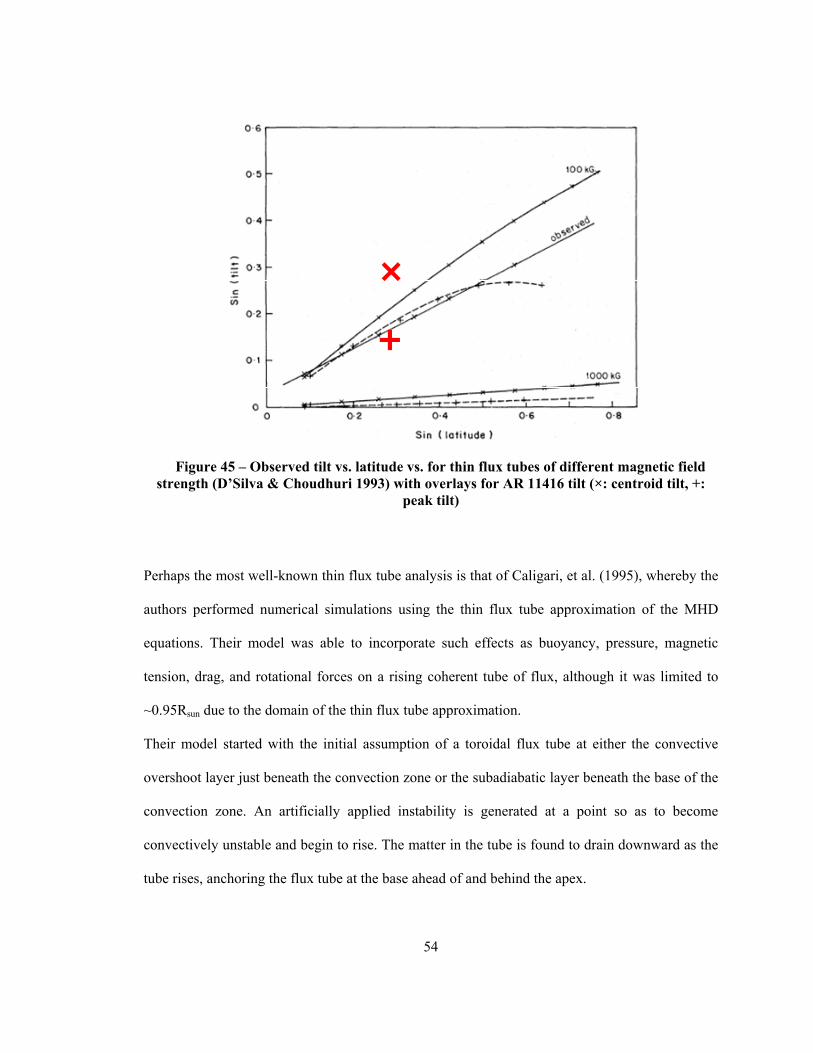
D’Silva and Choudhuri (1993) made use of the thin flux tube approximation to develop a model
specifically for purposes of investigating the source of the tilt of active regions. In their work,

53
they simulated a flux tube whose rise begins at the base of the convection zone and rises under
the influence of Coriolis force in a solid body rotation domain. In their study, they varied the
magnetic field strength, drag (implying changes in diameter), and anchor footprint separation at
the base of the tube.
Their primary finding was that in order to both buoyantly rise and produce tilt angles
corresponding to those seen in observations, the flux tube needed a field strength of 60 to 160 kG.
They also came to the conclusion that with decreases in footprint separation, magnetic tension of
the loop plays an increasing role to slow the flux tube’s ascent, thus exposing it to more influence
from the Coriolis force and producing a larger tilt.
Figure 45 shows the results of their computations versus observed values, with overlays for tilt
angle of the AR of interest in this current study. We included the tilt angles for both centroid and
peaks, since the tilt of the polarity peaks (darkest points) are more likely what others have
considered as part of their observations.
54
Figure 45 – Observed tilt vs. latitude vs. for thin flux tubes of different magnetic field strength (D’Silva & Choudhuri 1993) with overlays for AR 11416 tilt (×: centroid tilt, +:
peak tilt)
Perhaps the most well-known thin flux tube analysis is that of Caligari, et al. (1995), whereby the
authors performed numerical simulations using the thin flux tube approximation of the MHD
equations. Their model was able to incorporate such effects as buoyancy, pressure, magnetic
tension, drag, and rotational forces on a rising coherent tube of flux, although it was limited to
~0.95Rsun due to the domain of the thin flux tube approximation.
Their model started with the initial assumption of a toroidal flux tube at either the convective
overshoot layer just beneath the convection zone or the subadiabatic layer beneath the base of the
convection zone. An artificially applied instability is generated at a point so as to become
convectively unstable and begin to rise. The matter in the tube is found to drain downward as the
tube rises, anchoring the flux tube at the base ahead of and behind the apex.

55
One feature of the result was an asymmetry that developed in tube, whereby the apex of the flux
tube migrated in the direction opposite of rotation, developing an “asymmetric Λ” shape as
shown in Figure 46. The authors attributed this due to conservation of angular momentum due to
Coriolis force acting on a rising flux tube. Our observations see remarkable agreement with this
prediction, especially with respect to the motions of the flux peaks (see the section entitled
Apparent surface motion versus vertical emergence of 3D structure).
Figure 46 – Flux tube apex migration with time (left) and polar visualization (right) (Caligari, et al. 1995)
Another result produced by this model was the reproduction of the well known “Joy’s law” tilt of
ARs with respect to the equator. While our observation matched the tilt in the qualitative sense
(that is, leading polarity closer to the equator than the trailing), the tilt angle with respect to the
centroids of 18.5º was very different for our emergence latitude of 17ºS than the results obtained
from model runs originating in either the convective overshoot or the subadiabatic ranges. If,
however, we consider the tilt angle of the peak fluxes (~8º as contrasted to the 18.5º obtained

56
from use of centroids), which is probably more representative of historical observations, we see
some agreement with the assumption of origins in the subadiabatic region of the convection zone
(see Figure 47. Red X overlay denotes polarity tilt angle wrt peak fluxes; polarity tilt angle of
centroids is off-scale at 18.5º). This, according to the authors, would suggest a somewhat weaker
magnetic field than flux tubes anchored in the overshoot region.
Figure 47 – Results of thin flux tube simulation for origins in subadiabatic convection zone region (asterisks) and convective overshoot region (squares) (Caligari, et al. 1995).
Anelastic 3D MHD models
Although the thin flux tube approximation provides remarkable insight into the dynamics of the
flux tube as a whole, it fails to answer questions regarding the fine structure of the flux tube.
Specifically, it does not resolve the effects of plasma motions within the convection zone on the
coherence of the tube or the presence or absence of twist (and effects thereof) in the tube. For

57
these, we turn to the anelastic approximation. Like the thin flux tube approximation, anelastic
MHD breaks down just beneath the photosphere, where the speed of the rising flux tube ceases to
be much lower than the local Mach number (Abbett, et al. 2000). While a notable limitation of the
approximation, the computational expense of fully-compressible ideal MHD is cumbersome if not
outright prohibitive. Much work on developing these models has occurred in the past decade or
so, and we will examine a few of these relative to our observations.
Abbett, et al. (2000) employed this technique to examine the effects of twist on a tube of
magnetic flux originating at the base of a rectangular, adiabatically stratified domain spanning
5.147 pressure scale heights. These simulations varied the lateral size of the computational
domain, the initial length of the tube, the scale height, and the amount of twist initially present in
the flux tube. The authors did not include convective turbulence or Coriolis force in their
simulation.
Like previous studies, the authors came to the conclusion that a certain rate of twist is required to
prevent fragmentation as the flux tube ascended. However, they also determined that the flux
tubes shy of this critical twist value could remain coherent if the curvature of the rising loop was
increased. Unfortunately for our observations, the contours of our flux tube do not outright
suggest the presence of a twist in the field lines (nor reject it), at least not at the time of
emergence. To answer this question, the usage of full vector data is needed.
The Abbett, et al. (2000) paper goes further on to show how their simulations at the upper
boundary of their simulation would appear if viewed on a magnetogram. These results we can
directly compare to our observations. Figure 48 shows the results of two of the twisted flux tube
runs as compared to the observational results of the study.

58
Figure 48 – Abbett, et al. (2000) simulated magnetograms vs. observed
The observations do not seem to clearly show the “tails” of the flux polarities, which was a
feature of a rising, twisted flux tube as shown by the authors, although the “crescent” feature was
certainly present. Also, in spite of the previous remark that our 3D contour showed no indication
of twist, Abbett, et al., (2000) showed a final run that indicated a tilt on the magnetogram that was
introduced as a result of a higher twist level (q=0.25), to which our observations bear some
resemblance (see Figure 49).
t=22.9hr
t=45.8hr

59
Figure 49 – Abbett, et al., (2000) simulated magnetogram for high twist flux tube compared with observation
The authors published another paper in the following year based on the same model, except this
time with a modification of the anelastic momentum equation to include the noninertial -
2ρ0(Ω×v) term corresponding to effects of Coriolis force (Abbett, et al. 2001). Their simulation
domain varied the latitude and peak flux of flux tubes rising from its base. Unlike their previous
work, however, twist was not imparted onto the flux tube. The authors discovered that the
Coriolis force alone was able to prevent the tube from developing transverse flows and
fragmenting, alleviating the requirement for twist. This was a result of a strong axial flow along
the flux tube, which prevented the flux tube from generating transverse (north-south) counter-
rotating vortices resulting in a fragmentation of the flux tube seen in their 2000 work.
Another discovery from the newer model was that this axial flow was found to be counter the
direction of rotation. This flow was also found to be stronger in the trailing polarity. With
Coriolis force acting upon the asymmetry, the plasma moves preferentially towards the trailing
t=34.4hr

60
polarity, thus making it both more vertical and more coherent. This resulted in a shape not unlike
our “asymmetric Λ” and that of the thin flux tube simulations performed by Caligari, et al (1995)
(see Figure 50 for a reproduction of the “High Flux, Low Latitude” case results).
Figure 50 – Resultant flux tube shape from Abbet, et al (2001) (rotation in +x direction)
Their results also showed a migration of the leading polarity slightly more towards the equator
than the trailing polarity due to Coriolis force, further confirming the physical basis of Joy’s Law
and aligning with our model.
One of the authors of the above studies went on to publish another body of research in 2008 that
took the next step by applying the model to a rotating, spherical shell domain (Fan 2008). This
model simulated a solar convection zone in dimension, and the computational domain extended to
0.977Rsun, where the anelastic approximation is predicted to break down.

61
This model produced a curious result, in that a flux tube would rise cohesively when the twist of
the tube (right-handed in the northern hemisphere) was opposite the expected direction (left-
handed in the northern hemisphere) relative to observations of active regions cited by the author,
resulting in tilts opposite that of Joy’s law (Hale, et al. 1919). The Coriolis force, however,
countered this force, pushing tilt back in the expected direction. Thus, the author concluded that a
critical amount of twist opposite of that expected was required for both a cohesive rise while
allowing Coriolis force to dominate and produce a proper tilt.
The simulations produced a significant amount of fragmentation of the flux tube during its rise
during this “Low Negative Twist” case, losing significant amounts of flux during its ascent
(reproduced in Figure 51), no doubt a result of the lower cohesion afforded by the lower twist.

62
Figure 51 – Low Negative Twist case results (Fan 2008)
This result has some interesting comparisons to our observations. First, we see a clear analogy in
that we again see an “asymmetric Λ” shape encountered in the both the work of Caligari, et al.
(1995), as well as in our observation. Also like Caligari, et al. (1995) and our AR, there is one
more vertical leg of the flux tube, and one more inclined leg. We also see similarity in our AR in

63
that the more vertical leg is also the most cohesive, at least with respect to the magnetogram data
(see contrasting white light image in Figure 23). Where we see a marked difference is that Fan’s
(2008) model has this leg as the leading polarity, whereas our observations, the thin flux tube
model of Caligari, et al. (1995), and the work of Abbett, et al (2001) both have this as the trailing
polarity.
Fan (2008) also notes that there is an asymmetry in field strength between the leading and trailing
polarities, with the leading polarity being 1.23x as strong as the trailing leg. We, too, see a similar
disparity favoring the leading leg, although it is noticeably smaller (~1.14x). The author credits
this to the asymmetric stretching of the legs producing a greater divergence of flow along the
trailing leg (which is the less cohesive leg), driven by Coriolis force. A curious feature of our AR
is that, if Fan’s logic were to hold, then it would be the trailing polarity (the more vertical and
cohesive of the two) that should exhibit the greater peak field strength; clearly, this is not the
case.
Ideal MHD models at the photosphere
As time has progressed, so too has the speed of computational resources, enabling computational
modeling in the ideal MHD domain. This is of particular interest as modeling an emergence of
flux through the photosphere into the corona is now possible.
We turn our attention to the work of Manchester, et al (2004), where a horizontal flux tube is
simulated to rise from an initial location of 10 photospheric scale heights below the photosphere.
Upon breaching the photosphere boundary, a significant shear flow develops which causes the
polarities to initially emerge then separate along the latitude axis.

64
Figure 52 – Shear velocity in an emergent flux tube (Manchester, et al. 2004)
The authors attribute this shearing motion to the interaction of the Lorentz force with the
gravitational stratification of the corona. That is, forces driving it to expand within the corona
(whose density rapidly falls off) compete against those compressing it in a far denser solar
envelope.
What is remarkable about this result is that it offers an explanation for the complex tilt angle
evolution described in the AR Tilt Evolution section of this paper. Were the evolution due to
Coriolis force alone, we would expect progression of tilt angle in a constant direction as the loop
emerges. Instead, we clearly see the effects of this shearing force at work producing the reversal
in tilt angle after the initial sharp climb.
Modeling efforts published by Fang, et al (2010) reveal similar results, even after adding detail.
Here, the authors also used an ideal MHD model (the BATSRUS model developed by the

65
University of Michigan), although they included radiation terms, non-ideal equations of state, and
an empirical coronal heating model.

66
CHAPTER 5: SUMMARY In this study, we have presented a novel technique for visualization of active region emergence,
whereby magnetograms acquired from the Solar Dynamics Observatory were stacked vertically
to produce detailed contours of magnetic flux for active region NOAA 11416 as the region
emerged. The same high time resolution magnetograms were further processed to yield an
accurate figure for magnetic flux from the polarities. These data were further used to produce a
detailed mathematical model of flux emergence for 3D shape, tilt, flux polarity positions, and
motion of the AR for area-weighted flux centroid positions. We ultimately have determined the
flux tube to exhibit an “asymmetric Λ” shape with a complex tilt angle evolution. A summary of
relevant parameters can be found in Table 2. Comparisons to previous numerical simulations
shows that this AR has much in common with thin flux tube approximations with respect to the
overall shape and tilt of the AR, but comparisons with anelastic MHD simulations yield mixed
results. Comparisons to ideal, compressible MHD numerical solutions show that shear force
brought upon by differing Lorentz force contributions from sub-photospheric and coronal
motions provide a good explanation for the complex tilt angle evolution of the AR.

67
Table 2 – AR flux and geometric parameters summary
Parameter Value
Extrap. Peak Flux, + Polarity 7.89×10²¹ Mx
e‐folding time¹, + Polarity 13.1 hr
Peak Flux Injection Rate, + Polarity 1.53×10²⁰ Mx/hr
Extrap. Peak Flux, ‐Polarity ‐7.50×10²¹ Mx
e‐folding time¹, ‐ Polarity 12.6 hr
Peak Flux Injection Rate, ‐ Polarity ‐1.54×10²⁰ Mx/hr
Extrap. Max Polarity Separation 118 Mm
Max. Separation Velocity 0.408 km/s
e‐folding time 76.9 hr
Maximum 24.3°
Extrap. Final Angle 18.5°
Damping Constant of Oscillation 0.960
Natural Frequency of Oscillation 0.099 rad/hr
X‐Coord. Max Travel 10.9 Mm
X‐Coord. Extrap. Final Travel 5.07 Mm
X‐Coord. Damping Constant of Oscillation² 0.500
X‐Coord. Natural Frequency of Oscillation² 0.0977 rad/hr
Y‐Coord. Max Travel 4.29 Mm
Y‐Coord. Extrap. Final Travel 2.76 Mm
+ Polarity, 0.1 km/s rise rate 60.7°
‐ Polarity, 0.1 km/s rise rate ‐52.4°
¹ ‐ e‐folding time is for half of injection
² ‐ Only X‐coordinate motion determined ζ and ω₀; Y was assumed l inear
Flux
Polarity Separation
Tilt of Polarity Centroids
Center Motion
Overall "Λ" Leg Angles

68
REFERENCES

69
REFERENCES
Abbett, W. P., Fisher, G. H., Fan, Y. 2000, The Astrophysical Journal 540: 548-562 Abbett, W. P., Fisher, G. H., Fan, Y. 2001, The Astrophysical Journal 546: 1194-1203 Caligari, P., Moreno-Insertis, F., Schüssler, M. 1995, The Astrophysical Journal 441: 886-902 Cheung, M. C. M., Rempel, M., Title, A. M., Schüssler, M. 2010, The Astrophysical Journal 720: 233-244 Choudhuri, A. H., Schüssler, M., Dikpati, M. 1995, Astronomy and Astrophysics, 303: L29-L32 D’Silva, S., Choudhuri, A. R. 1993, Astronomy and Astrophysics 272: 621-633 Manchester IV, W., Gombosi, T., DeZeeuw, D., Fan, Y. 2004, The Astrophysical Journal 610: 588-596 Fan, Y. 2008, The Astrophysical Journal 676: 680-697 Fan, Y. 2009, The Astrophysical Journal 697: 1529-1542 Fan, Y. 2009, Living Reviews in Solar Physics, 6, 4 Fang, F., Manchester IV, W., Abbet, W. P., van der Holst, B. 2010, The Astrophysical Journal 714: 1649-1657 Hale, G. E., Ellerman, F., Nicholson, F. B., Joy, A. H. 1919, The Astrophysical Journal 49: 153 HMI Team. 2012, HMI Overview (Stanford, CA:Stanford Solar Group), http://hmi.stanford.edu/Description/HMI_Overview.pdf Leka, K. D., Canfield, R. C., McClymont, A. N., van Driel-Gesztelyi, L. 1996, The Astrophysical Journal 462: 547-560 Longcope, D. W., Fisher, G. H. 1996, The Astrophysical Journal, 458: 380-390 Longcope, D. W., Fisher, G. H., Pevtsov, A. A. 1998, The Astrophysical Journal, 507: 417-432 Pesnell, W. D., Thompson, B. T., Chamberlin, P. C. 2012, Solar Physics, 275: 3-15

70
Tanaka, K. 1991, Solar Physics 136: 133-149 Tóth, L., Gerlei. 2003, Publications of the Astronomy Department of the Eötvös University, 13: 95-100 Schou, J., Scherrer, P. H., Bush, R. I., et al. 2012, Sol. Phys., 275: 229 Zwaan, C. 1985, Solar Physics, 100: 397-414 Zwaan, C. 1987, Astronomy and Astrophysics, 25: 83-111

71
CURRICULUM VITAE
Mr. Brian Briggs has been a student at the George Mason University since 2008. He began his education at the University of Central Florida, receiving a Bachelor of Science in Mechanical Engineering in 2003. Since receiving his BSME, Brian has worked for Swales Aerospace (presently ATK Space Systems) and Orbital Sciences Corporation as a thermal engineer, developing and testing thermal control subsystems for high-altitude research balloons as well as numerous scientific, technology demonstration and telecommunications spacecraft. Brian returned to school for graduate study in 2008, whereupon his studies have focused on astronomy and astrophysics, culminating in solar physics research with Dr. Jie Zhang in 2012.