determination of natural frequencies and mode shapes of a ... · timoshenko beam, the stiffness...

Wind Energ. Sci., 4, 57–69, 2019https://doi.org/10.5194/wes-4-57-2019© Author(s) 2019. This work is distributed underthe Creative Commons Attribution 4.0 License.

Determination of natural frequencies and modeshapes of a wind turbine rotor blade using

Timoshenko beam elements

Evgueni Stanoev and Sudhanva Kusuma ChandrashekharaFaculty of Mechanical Engineering and Marine Technology, Endowed Chair of Wind Energy Technology,

University of Rostock, Rostock, 18059, Germany

Correspondence: Evgueni Stanoev ([email protected])

Received: 26 September 2018 – Discussion started: 15 October 2018Revised: 11 December 2018 – Accepted: 2 January 2019 – Published: 28 January 2019

Abstract. When simulating a wind turbine, the lowest eigenmodes of the rotor blades are usually used to de-scribe their elastic deformation in the frame of a multi-body system. In this paper, a finite element beam modelfor the rotor blades is proposed which is based on the transfer matrix method. Both static and kinetic field matri-ces for the 3-D Timoshenko beam element are derived by the numerical integration of the differential equationsof motion using a Runge–Kutta fourth-order procedure. In the general case, the beam reference axis is at anarbitrary location in the cross section. The inertia term in the motion differential equation is expressed usingappropriate shape functions for the Timoshenko beam. The kinetic field matrix is built by numerical integrationapplied on the approximated inertia term. The beam element stiffness and mass matrices are calculated by simplematrix operations from both field matrices. The system stiffness and mass matrices of the rotor blade model areassembled in the usual finite element manner in a global coordinate system accounting for the structural twistangle and possible pre-bending. The program developed for the above-mentioned calculations and the final so-lution of the eigenvalue problem is accomplished using MuPAD, a symbolic math toolbox in MATLAB®. Thenatural frequencies calculated using generic rotor blade data are compared with the results proposed from theFAST and ADAMS software.

1 Introduction

Vibration of an elastic system refers to a limited reciprocat-ing motion of a particle or an object of the system. Windturbines operate in an unsteady environment which results ina vibrating response (see Manwell et al., 2009). They consistof long slender structures (rotor blades and tower), which re-sult in resonant frequencies that should be taken into accountduring the initial design and construction. When the excita-tion frequency of the vibrating system is near any natural fre-quency, an undesirable resonant state occurs with large am-plitudes, which may lead to damage or even the collapse ofthe wind turbine or its components. The vibration response,especially of the rotor blades, depends on the stiffness whichis a function of the materials used, the design and the size(see Jureczko et al., 2005). Therefore, the estimation of nat-

ural frequencies in the early design phase plays an importantrole in avoiding resonance.

The eigenmodes associated with the lowest natural fre-quencies are employed as shape functions to describe theelastic deformation of the rotor blade beam model in theframe of the usual simulation of the wind turbine as a multi-body system. Generally, the first two bending eigenmodesin each direction (flapwise and edgewise) and optionally thetwo additional torsional eigenmodes are used. The determi-nation of the lowest eigenmodes with sufficient numericalaccuracy is the first step with respect to the modal superposi-tion applied to the deformational motion of the rotor blades.

Due to the geometrical complexity of the blade cross sec-tion profiles and the extended use of composite materials, theexact calculation of natural frequencies in the design processtakes a considerable amount of time and financial expense

Published by Copernicus Publications on behalf of the European Academy of Wind Energy e.V.

58 E. Stanoev and S. Kusuma Chandrashekhara: Natural frequencies and mode shapes of wind turbine rotor blades

with regards to the 3-D modelling of the rotor blade usingCAD software; hence a simplified finite element beam modelis necessary. A twisted rotor blade is simplified into a can-tilever beam with a non-uniform cross section. The structuraltwist angle is implemented by changing the orientation of theprincipal axis of the blade cross section along the length ofthe blade.

In the finite element formulation of beams two linear beamtheories are established, the Euler–Bernoulli beam model andthe Timoshenko beam model. Although the Euler–Bernoullibeam theory is widely used, the Timoshenko beam theory isconsidered to be better as it incorporates the effects of trans-verse shear and the rotational inertia on the dynamic responseof the beam (see Kaya, 2006). In the classical approach of thefinite element formulation for the free vibration analysis ofbeams, the stiffness and mass matrices are derived using in-terpolation functions derived from second- and fourth-orderHermite polynomials. The stiffness matrix is derived fromthe following equation (see Wu, 2013):

K (e) =∫

BTDmBdv, (1)

where K (e) is the element stiffness matrix, B is the strain ma-trix and Dm is the elasticity matrix for the beam. The elementmass matrix of the beam (see Wu, 2013) is derived using thefollowing equation:

M (e)=∫ρaTadv, (2)

where M (e) is the element mass matrix, ρ is the mass den-sity, v is the volume and a is the matrix of interpolation func-tions.

Using the above-mentioned standard relations and appro-priate shape functions for the Euler–Bernoulli beam and theTimoshenko beam, the stiffness matrix and consistent massmatrix for the finite beam element can be derived. However,an alternative to this procedure, based on the transfer matrixmethod for the beam theory (see Graf and Vassilev, 2006:69–88 and Stanoev 2007) is developed in the present article.The element stiffness matrix can be derived on the basis ofnumerical integration of the first-order ordinary differentialequation system for the differential beam element. The asso-ciated mass matrix can be developed by numerical integra-tion of the inertia term in the differential equation of motion.The numerical integration results in static and kinetic fieldmatrices, from which the element stiffness and mass matri-ces can be easily assembled.

In the present article, the above-mentioned procedure isused to determine the element stiffness and element massmatrix for the Timoshenko beam. The interpolation functionsused for deriving the mass matrix are based on Hermite poly-nomials according to Bazoune and Khulief (2003). The sys-tem stiffness and mass matrices for the rotor blade are assem-bled in a global coordinate basis in the usual finite element

manner. The numerical solution of the associated eigenvalueproblem for the system without damping is computed usingcomputer algebra software (in the frame of MATLAB®).

In Sects. 2 and 3, the proposed method is described in de-tail; in Sect. 4 the method is applied on a rotor blade struc-ture with 288 degrees of freedom (DOFs). The results forthe natural frequencies and the corresponding eigenmodesare compared with the results calculated using the FAST andADAMS software.

2 Theoretical framework for the 3-D Timoshenkobeam

2.1 Kinematic relationships

The general assumptions in the linear beam theory are as fol-lows:

a. The beam reference (longitudinal) axis is at any arbi-trary location of the cross section.

b. The only stresses that occur are normal stresses σx andshear stresses τxy , τxz.

c. Cross section planes, which are initially normal to thelongitudinal axis, will remain plane after deformation.

The geometrical representation of the deformation state of abeam cross section is shown in the Fig. 1. The deformationsup, vp and wp at a cross-sectional point P are determined bythree displacement functions u(x), v(x) and w(x) and threecross-sectional rotation angles ϕx(x), ϕy (x) and ϕz(x) – allof them are a function of the beam axis coordinate x. The dif-ferential equation system is derived in accordance with Sta-noev (2013):

As seen in Fig. 1, the displacement vector up can be ex-pressed at any cross section point P as

up =

[up (x,y,z)vp (x,y,z)wp (x,y,z)

]=

[u (x)− yϕz (x)+ zϕy (x)

v (x)− zϕx (x)w (x)+ yϕx (x)

](3)

The three components of the strains occurring in the beamcan be expressed as the derivatives of the displacement func-tions up, vp and wp. The axial strain εxx and the two shearstrain components γxz and γxy are given by the following:

εxx =∂up

∂x= u′− yϕ′z+ zϕ

′y (4a)

γxz =∂up

∂z+∂wp

∂x= ϕy +w

′︸︷︷︸γy

+ yϕ′x (4b)

γxy =∂up

∂y+∂vp

∂x=−ϕz+ v

′︸︷︷︸γy

− zϕ′x, (4c)

where γz and γy are the constant shear strains that are notneglected in Timoshenko beam theory.

γy =−ϕz+ v′ (5a)

γz = ϕy +w′ (5b)

Wind Energ. Sci., 4, 57–69, 2019 www.wind-energ-sci.net/4/57/2019/

E. Stanoev and S. Kusuma Chandrashekhara: Natural frequencies and mode shapes of wind turbine rotor blades 59

Figure 1. Deformation at the point (x,y,z) (see Andersen and Nielsen, 2008).

2.2 Principle of virtual work for internal forces

The virtual work components for internal forces correspond-ing to normal stresses and shear stresses are given by the fol-lowing:

−δWi =

∫x

{δu′N + δϕ′zMz+ δϕ

′yMy

}dx+

∫x

{δγzQz}dx

+

∫x

{δγyQy

}dx+

∫x

{δϕ′xMTP

}dx, (6)

where N is the axial force, Mz and My are bending internalmoments,Qy andQz are the corresponding shear forces andMTP is the St. Venant torsional moment.

With the introduction of the constitutive relations ofHooke’s material law for the stresses corresponding to theinternal forces in Eq. (6) and expressing the strains usingEqs. (4a)–(4c) and (5a)–(5b), the virtual work relationshipis reformulated as

−δWi=

∫x

{E

∫A

dA

︸︷︷︸

A

· u′−

∫A

ydA

︸︷︷︸

Ay

·ϕ′z +

∫A

zdA

︸︷︷︸

Az

·ϕ′y

δu′

−E

∫A

ydA

︸︷︷︸

Ay

· u′−

∫A

y2dA

︸︷︷︸

Ayy

·ϕ′z +

∫A

yzdA

︸︷︷︸

Ayz

·ϕ′y

δϕ′z

+E

∫A

zdA

︸︷︷︸

Az

· u′−

∫A

yzdA

︸︷︷︸

Ayz

·ϕ′z +

∫A

z2dA

︸︷︷︸

Azz

·ϕ′y

δϕ′y

+G

[Asz

(w′+ϕy

)δw′+Asz(w′+ϕy )δϕy

+Asy(v′−ϕz

)δv′−Asy (v′−ϕz)δϕz

]

+G

∫A

(z2+ y2)dA

︸︷︷︸

IT

ϕ′xδϕ′x

}dx (7)

Here,Asz = αsz·A andAsy = αsy ·A are the shear areas in thez and y directions respectively, αsz, αsy are the correspondingshear correction coefficients, A is the cross-sectional area,Ay is the static moment with respect to the z axis, Az is thestatic moment with respect to the y axis, Ayy is the momentof inertia with respect to the z direction, Azz is the momentof inertia with respect to the y direction, Ayz is the deviationmoment of inertia and IT is the torsional moment of inertia.

After the coefficient comparison in Eqs. (6) and (7) theinternal forces corresponding to the normal stresses can beexpressed by introducing the cross sectional stiffness matrixEA: N

−Mz

My

= EA EAy EAzEAy EAyy EAyzEAz EAyz EAzz

︸︷︷︸

EA

·

u′

−ϕ′zϕ′y

⇒

u′

−ϕ′zϕ′y

= (EA)−1

N

−Mz

My

(8)

The shear stress components in Eqs. (6) and (7) lead to thefollowing relations:

Mx =MTP =GITϕ′x (9)

Qz =GAsz(w′+ϕy

)(10a)

Qy =GAsy(v′−ϕz

)(10b)

www.wind-energ-sci.net/4/57/2019/ Wind Energ. Sci., 4, 57–69, 2019


The relation described in Eq. (10a) and (10b) implies that thechosen reference axis coincides with the shear centre due toneglected shear–torsion coupling terms in Eq. (7).

For the special case where the cross section coordinatesystem coincides with the principal axes, the deformation re-lationship in Eq. (8) reduces to N

−Mz

My

= EA 0 0

0 EAYY 00 0 EAzz

· u′

−ϕ′zϕ′y

⇒

u′

−ϕ′zϕ′y

= (EA)−1

N

−Mz

My

(11)

2.3 Differential equation system

The virtual work relation in Eq. (7) is rewritten for the casewhere the beam coordinate system coincides with the princi-pal axis of the cross section – see Eq. (11).

−δWi =

∫x

{(EAu′

)δu′+

(EAyyϕ

′z

)δϕ′z+

(EAzzϕ

′y

)δϕ′y

+ (GITϕ′x)δϕ′x +GAsz

(w′+ϕy

)(δw′+ δϕy)

+GAsy(v′−ϕz

)(δv′− δϕz

)}dx (12)

After the partial integration of Eq. (12) the cross section de-formation relations and differential equilibrium conditionsfor the Timoshenko beam element are compiled in a first-order differential equation system (see Eqs. 13, 14). For theTimoshenko beam with an arbitrary beam reference axis atany point on the cross section (see Eq. 8), the system of dif-ferential equations can be expressed in the following form:

ddx

uvwϕxϕyϕzNQy

Qz

Mx

My

Mz

=

0 0 0 0 0 0 S11 0 0 0 S13 −S12

0 0 0 0 0 1 01

GAsy0 0 0 0

0 0 0 0 −1 0 0 01

GAsz0 0 0

0 0 0 0 0 0 0 0 01GIT

0 0

0 0 0 0 0 0 S31 0 0 0 S33 −S320 0 0 0 0 0 −S21 0 0 0 −S23 S220 0 0 0 0 0 0 0 0 0 0 00 0 0 0 0 0 0 0 0 0 0 00 0 0 0 0 0 0 0 0 0 0 00 0 0 0 0 0 0 0 0 0 0 00 0 0 0 0 0 0 0 1 0 0 00 0 0 0 0 0 0 −1 0 0 0 0

·

uvwϕxϕyϕzNQy

Qz

Mx

My

Mz

+

000000−px−py−pz−mT−my−mz

(13)

The differential equation system for the Timoshenko beamwith the beam reference axis on principal axes can be repre-sented in the following matrix form:

ddx

uvwϕxϕyϕzNQy

Qz

Mx

My

Mz

=

0 0 0 0 0 01EA

0 0 0 0 0

0 0 0 0 0 1 01

GAsy0 0 0 0

0 0 0 0 −1 0 0 01

GAsz0 0 0

0 0 0 0 0 0 0 0 01GIT

0 0

0 0 0 0 0 0 0 0 0 01

EAzz0

0 0 0 0 0 0 0 0 0 0 01

EAzz0 0 0 0 0 0 0 0 0 0 0 00 0 0 0 0 0 0 0 0 0 0 00 0 0 0 0 0 0 0 0 0 0 00 0 0 0 0 0 0 0 0 0 0 00 0 0 0 0 0 0 0 1 0 0 00 0 0 0 0 0 0 −1 0 0 0 0

·

uvwϕxϕyϕzNQy

Qz

Mx

My

Mz

+

000000−px−py−pz−mT−my−mz

(14)

The entries Sij in Eq. (13) are determined by the inversion ofthe cross-sectional stiffness matrix in Eq. (8): u′

−ϕ′zϕ′y

= EA EAy EAz

EAy EAyy EAyzEAz EAyz EAzz

−1

︸︷︷︸S

·

N

−Mz

My

=

S11 S12 S13S21 S22 S23S31 S32 S33

︸︷︷︸

S

·

N

−Mz

My

(15)

3 Alternative finite element formulation

In the classical finite element formulation, the beam stiff-ness matrix and the consistent beam mass matrix are de-rived by developing an approach for the displacement func-tions through shape (interpolation) functions, which consistof first- and third-order Hermite polynomials. In this section,an alternative finite element procedure is presented, based onthe numerical Runge–Kutta fourth-order integration of thedifferential motion equations. The integration of the staticpart (the coefficient matrix in Eqs. 13 and 14 respectively)leads to the static field matrix, while the integration of theinertia terms in the equation of motion Eq. (16) results in a



Figure 2. The finite beam element: internal forces and nodal DOFs.

kinetic field matrix. In the last step of the integration, usingboth field matrices, the respective element stiffness and theelement mass matrices can be calculated using simple matrixoperations.

3.1 The differential equations of motion

The differential equations of motion for the differential beamelement (see Fig. 2) can be written in a matrix form accordingto Stanoev (2007) and Müller (2012) as follows:[z1,xz2,x

]=

[A11 A12A21 A22

]︸︷︷︸

A

·

[z1z2

]+

[b1b2

]

+

[0m

]· z1 (16)

In the above-mentioned equation, matrix A is the coefficient

matrix (see Eqs. 13, 14) and vector z=[z1z2

]is the state

vector, where

z1=[u (x) v (x) w (x) ϕx (x) ϕy (x) ϕz (x)

]Tis the vector of the displacement functions, and (16a)

z2=[N (x) Qy (x) Qz (x) Mx (x) My (x) Mz (x)

]Tis the vector of internal (section) force functions. (16b)

The vector b =[b1b2

]contains the known excitation forces;

however, for an eigenvalue problem b = 0. The coefficientmatrix A and the state vector z in addition to excitation forceb constitute the static part of the motion equation. The kineticpart of the motion equation can be expressed using a matrixof the interpolation functions and nodal acceleration vectoras follows:[

0m

]· z1 =

[0m

][81(x) 82(x)]︸︷︷︸

bm

·

[V (a)V (b)

]︸︷︷︸V R(e,t)

, (17)

where z1 =[u v w ϕx ϕy ϕz

]T is the vector of ac-celerations, [81 (x) 82 (x)]εR(6×12) is the matrix of inter-polation functions (see Sect. 3.3), V (a) , V (b) εR(6×1) is thevector with nodal accelerations and mεR(6×6) is the inertiamatrix of the differential beam element (see Sect. 3.2).

3.2 The inertia matrix term

The inertia matrix in Eq. (18) implies that the distributedmass µ (x) (kg m−1) is applied eccentrically at any location(y,z) in the cross section. The inertia matrix is expressed ac-cording to Stanoev (2013):

m= µ ·

1 0 0 0 z −y0 1 0 −z 0 00 0 1 y 0 0

0 −z y (y2+ z2+2p

µ) 0 0

z 0 0 0 (z2+2y

µ) −yz

−y 0 0 0 −yz (y2+2z

µ)

, (18)

where 2p, 2y and 2z in (kg m) are the mass moments ofinertia for the cross section.

2y =µ · Iy

A=µ ·Azz

A, 2z =

µ · Iz

A=µ ·Ayy

A,

2p =2y +2z (19)

3.3 Shape functions for the Timoshenko beam element

The acceleration term z1 in Eq. (17) is expressed using theproduct of Hermite interpolating polynomials and the nodalacceleration vectors V (a) and V (b).

Shape functions for axial and torsional deformations u (ξ )and ϕx (ξ ), respectively, are derived using first-order polyno-mial as follows:

u (ξ )= a1+ a2ξ = [1 ξ ]︸︷︷︸Nu

[a1a2

]︸︷︷︸a

=Nu · a, ξ =x

L(20)

To express the coefficients aj in terms of the nodal dis-placements u (ξ = 0)= ua , u (ξ = 1)= ub or in terms of the



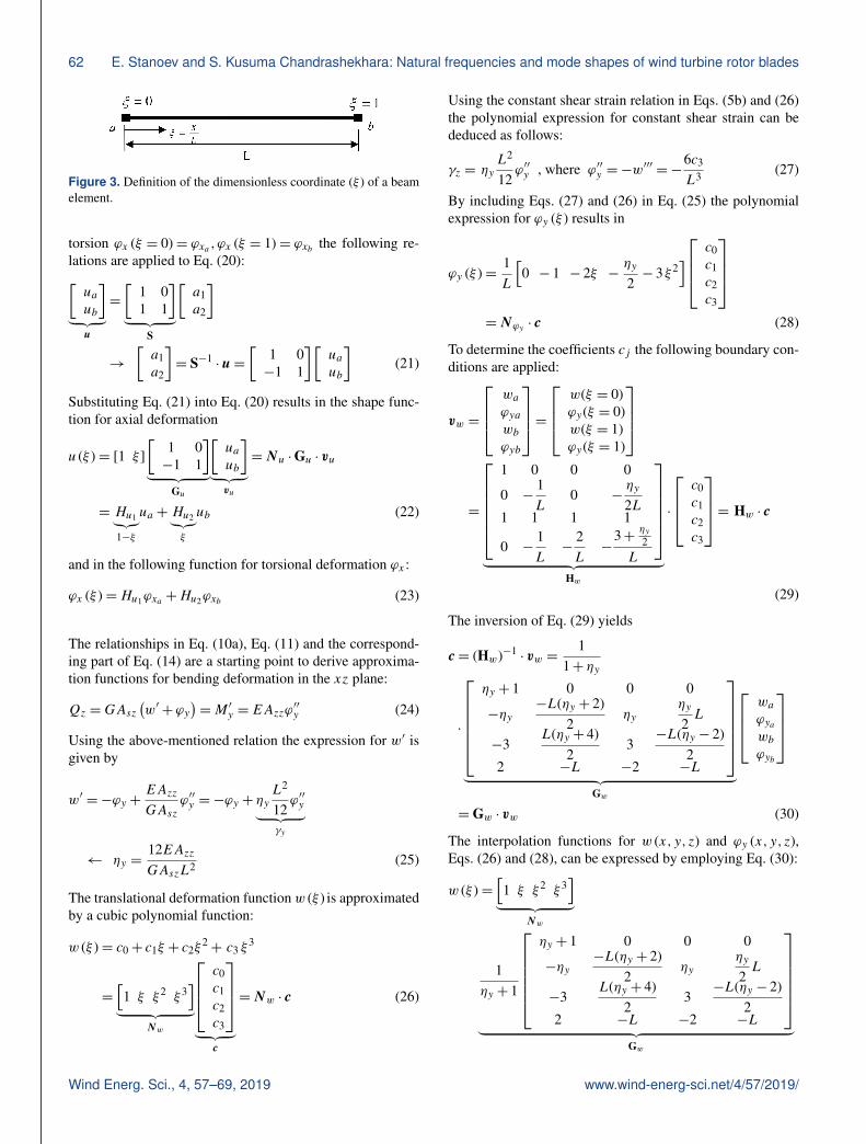
Figure 3. Definition of the dimensionless coordinate (ξ ) of a beamelement.

torsion ϕx (ξ = 0)= ϕxa ,ϕx (ξ = 1)= ϕxb the following re-lations are applied to Eq. (20):[uaub

]︸︷︷︸

u

=

[1 01 1

]︸︷︷︸

S

[a1a2

]

→

[a1a2

]= S−1

·u=

[1 0−1 1

][uaub

](21)

Substituting Eq. (21) into Eq. (20) results in the shape func-tion for axial deformation

u (ξ )= [1 ξ ][

1 0−1 1

]︸︷︷︸

Gu

[uaub

]︸︷︷︸vu

=Nu ·Gu · vu

= Hu1︸︷︷︸1−ξ

ua + Hu2︸︷︷︸ξ

ub (22)

and in the following function for torsional deformation ϕx :

ϕx (ξ )=Hu1ϕxa +Hu2ϕxb (23)

The relationships in Eq. (10a), Eq. (11) and the correspond-ing part of Eq. (14) are a starting point to derive approxima-tion functions for bending deformation in the xz plane:

Qz =GAsz(w′+ϕy

)=M ′y = EAzzϕ

′′y (24)

Using the above-mentioned relation the expression for w′ isgiven by

w′ =−ϕy +EAzz

GAszϕ′′y =−ϕy + ηy

L2

12ϕ′′y︸︷︷︸

γy

← ηy =12EAzzGAszL2 (25)

The translational deformation functionw (ξ ) is approximatedby a cubic polynomial function:

w (ξ )= c0+ c1ξ + c2ξ2+ c3 ξ

3

=

[1 ξ ξ2 ξ3

]︸︷︷︸

Nw

c0c1c2c3

︸︷︷︸

c

=Nw · c (26)

Using the constant shear strain relation in Eqs. (5b) and (26)the polynomial expression for constant shear strain can bededuced as follows:

γz = ηyL2

12ϕ′′y , where ϕ′′y =−w

′′′=−

6c3

L3 (27)

By including Eqs. (27) and (26) in Eq. (25) the polynomialexpression for ϕy (ξ ) results in

ϕy (ξ )=1L

[0 − 1 − 2ξ −

ηy

2− 3ξ2

]c0c1c2c3

=Nϕy · c (28)

To determine the coefficients cj the following boundary con-ditions are applied:

vw =

waϕyawbϕyb

=w(ξ = 0)ϕy(ξ = 0)w(ξ = 1)ϕy(ξ = 1)

=

1 0 0 0

0 −1L

0 −ηy

2L1 1 1 1

0 −1L−

2L−

3+ ηy2

L

︸︷︷︸

Hw

·

c0c1c2c3

= Hw · c

(29)

The inversion of Eq. (29) yields

c = (Hw)−1· vw =

11+ ηy

·

ηy + 1 0 0 0

−ηy−L(ηy + 2)

2ηy

ηy

2L

−3L(ηy + 4)

23−L(ηy − 2)

22 −L −2 −L

︸︷︷︸

Gw

waϕyawbϕyb

=Gw · vw (30)

The interpolation functions for w (x,y,z) and ϕy (x,y,z),Eqs. (26) and (28), can be expressed by employing Eq. (30):

w (ξ )=[1 ξ ξ2 ξ3

]︸︷︷︸

Nw

1ηy + 1

ηy + 1 0 0 0

−ηy−L(ηy + 2)

2ηy

ηy

2L

−3L(ηy + 4)

23−L(ηy − 2)

22 −L −2 −L

︸︷︷︸

Gw


E. Stanoev and S. Kusuma Chandrashekhara: Natural frequencies and mode shapes of wind turbine rotor blades 63waϕyawbϕyb

︸︷︷︸

vw

=Hw1wa +Hw2ϕya +Hw3wb+Hw4ϕyb , (31)

where the products of both matrices Nw and Gw are intro-duced as functions Hwj (j = 1, . . .,4).

ϕy (ξ )=1L

[0− 1− 2ξ −

ηy

2− 3ξ2

]︸︷︷︸

Nϕy

1ηy + 1

ηy + 1 0 0 0

−ηy−L(ηy + 2)

2ηy

ηy

2L

−3L(ηy + 4)

23−L(ηy − 2)

22 −L −2 −L

·waϕyawbϕyb

=Hϕy1

wa +Hϕy2ϕya +Hϕy3

wb+Hϕy4ϕyb (32)

In Eq. (32), the functions Hϕyj (j = 1, . . .,4) are introducedin an analogous manner.

A similar method is used for determining the approxima-tion functions v (ξ ) and ϕz (ξ ) for bending deformation in thexy plane.

Starting with Eqs. (10b), (11) and (14), the following isobtained:

Qy =GAsy(v′−ϕz

)=−M ′z =−EAyyϕ

′′z (33)

v′ = ϕz−EAyy

GAsyϕ′′z = ϕz+ ηz

L2

12ϕ′′z

← ηz =12EAyyGAsyL2 (34)

The approximations analogous to Eqs. (31) and (32) can bederived as follows:

v (ξ )=Hv1va +Hv2ϕza +Hv3vb+Hv4ϕzb (35)ϕz (ξ )=Hϕz1 va +Hϕz2ϕza +Hϕz3 vb+Hϕz4ϕzb (36)

TheH∗j functions developed in Eqs. (31), (32), (35) and (36)are “static” shape functions for the Timoshenko beam. Sup-posing dependence on time alone for the nodal displacementvectors V (a) and V (b), the matrix of the interpolation func-tions [81 (x) 82 (x)] in the inertia term Eq. (17) can be de-veloped using Eqs. (31), (32), (35) and (36) (see KusumaChandrashekhara, 2018):

81(x)=

Hu1 0 0 0 0 0

0 Hv1 0 0 0 Hv20 0 Hw1 0 Hw2 00 0 0 Hu1 0 00 0 Hϕy1

0 Hϕy20

0 Hϕz10 0 0 Hϕz2

,

82(x)=

Hu2 0 0 0 0 0

0 Hvs 0 0 0 Hv40 0 Hws 0 Hw4 00 0 0 Hu2 0 00 0 Hϕys 0 Hϕy4

00 Hϕzs 0 0 0 Hϕz4

, (37)

3.4 Numerical integration

The special form of the numerical Runge–Kutta fourth-orderintegration method applied here is described in detail inMüller and Wolf (1975) and Schenk (2012). The integrationoperator is applied to the equations of motion in Eq. (16), i.e.[z1,xz2,x

]= A ·

[z1z2

]+

[b1b2

]+

[0m

][81(x) 82(x)]︸︷︷︸

bm

· V R (e, t) (38)

In order to gain sufficient numerical precision the beam axisneeds to be divided into at least 20 integration intervals. Theintegration operator transfers the known state vector at be-ginning of the integration interval to the end of the interval.The integration procedure starts with the state vector at thefirst node a, i.e. at location (x = 0):[z1(x = 0)z2(x = 0)

]︸︷︷︸

z(a)

=

1· · ·

1

z (a) (39)

The integration operator is subsequently applied to the eval-uated coefficient matrix A at each interval by excluding theinitial state vector z (a). The result are static field matricesF (x,a), multiplicatively linked to z (a) see Eq. (40). There-fore, each F (x,a) matrix “transfers” the state vector at loca-tion (x = 0) to the end x of the integration interval considered(transfer matrix method). In the frame of the integration pro-cedure the actual field matrix F (x,a) serves column wise asan initial vector for the next interval, and the components ofthe state vector z (a) remain excluded. The beam “load” vec-

tor[b1b2

], Eq. (38), evaluated in the actual interval, yields

the

β1β21

column in the F (x,a) matrix after integration –

Eq. (40).The numerical integration of the inertia term bm in

Eq. (38) is carried out column wise analogously to the “load”vector, by excluding the nodal accelerations V R (e, t) – theresults are kinetic field matrices H (x,a) at the end of eachintegration interval (at location x) (see Eq. 40):[

z1(x)z2(x)

1

]︸︷︷︸=

[α11 α12 β1α21 α22 β20 0 1

]︸︷︷︸ ·

[z1(a)z2(a)

1

]

z(x)= F(x,a) · z(a)



Figure 4. Eccentrically applied mass mE at the xAE point of the beam in the 3-D case.

Figure 5. First flapwise eigenmode.

+

[H11 H12 0H21 H22 0

0 0 1

]︸︷︷︸ ·

V (a)V (b)

0

+H(x,a) · V R(e)

(40)

This type of numerical integration allows (slightly) varyingvalues of the coefficients of the A matrix, the bm inertia termand the b vector along the beam axis – i.e. all stiffness, massand external load values of the beam element may vary. Af-ter the last integration step at the second node b, at location(x = L), static L (e) and kinetic H (e) field matrices are ob-tained: z1(b)z2(b)

1

= L(e) ·

z1(a)z2(a)

1

+H(e) ·

V (a)V (b)

0

(41a)

Figure 6. First edgewise eigenmode.

where

L(e)=

L11 L12 f 1L21 L22 f 20 0 1

,H(e)=

H11 H12 0H21 H22 0

0 0 1

(41b)

According to Eqs. (13) and (14) the state variable z1 rep-resents six-component displacement vectors for V (a) andV (b), respectively, and the state variable z2 represents six-component internal forces vectors S (a) and S (b), at loca-tions (x = 0) and (x = L) respectively.



Figure 7. Second flapwise eigenmode.

3.5 The element stiffness and mass matrices

By solving the matrix equation in Eq. (41a) for S (a) andS (b), and accounting for the definitions of internal forces infinite element beam formulation (see Fig. 2),

F (a)=−S (a) , F (b)= S (b) , (42)

one can derive the element stiffness matrix K (e), the elementmass matrix M (e) and the element forces and moments F 0

using simple matrix operations as shown in Eq. (43). Thenthe beam element relationships for the internal forces can beformulated as[F (a)F (b)

]=

[F 0(a)F 0(b)

]+

[Kaa Kab

Kba Kbb

]︸︷︷︸

K(e)

·

[V (a)V (b)

]

+

[Maa Mab

Mba Mbb

]︸︷︷︸

M(e)

·

[V (a)V (b)

]=

[L−1

12 ·f 1f 2−L22 ·L−1

12 ·f 1

]︸︷︷︸

F0

+

[L−1

12 ·L11 −L−112

L21−L22 ·L−112 ·L11 L22 ·L−1

12

]︸︷︷︸

K(e)

·

[V (a)V (b)

]

+

[L−1

12 ·H11 −L−112 ·H12

H21−L22 ·L−112 ·H11 H22−L22 ·L−1

12 ·H12

]︸︷︷︸

M(e)

·

[V (a)V (b)

](43)

Figure 8. Mixed flap/edgewise eigenmode.

3.6 Single masses at eccentric positions

The numerical integration according to Runge–Kutta, de-scribed in Sec. 3.4, offers the possibility of including sin-gle load or mass quantities within a beam element. Singleeccentric masses can be taken into account at the integra-tion interval boundaries. In the local coordinate system of thebeam element, at a general position vector xAE =

[yE zE

]T,the eccentric mass and the vector representation of dynamicequilibrium, Eq. (44a)–(44b), is as shown in Fig. 4. The beamreference axis is at point A, and vector V E represents the ac-celeration vector at the point of application (x,xAE). Withthe help of the dynamic equilibrium conditions Eq. (44a)–(44b), additional inertia forces and moments due to eccentricmass can be determined (see Li, 2016):

−NL+NR =mEV E (44a)

ML+MR =

3∑i=1

(θEi ϕiei)+(xAE ×mEV E

), (44b)

where NL and NR are internal force vectors on the left andright in differential proximity to the point at location x, ML

and MR are internal moment vectors on the left and right indifferential proximity to the point at location x (see Fig. 4),mE is the eccentric single mass, 2Ei are the mass momentsof inertia of the single mass and ϕi are the angular accelera-tions at location x.



Figure 9. First torsional eigenmode.

The additional inertia matrix ME (mE,2Ei, x,xAE), de-rived from Eq. (44a)–(44b), is analogous to the inertia ma-trix due to distributed mass in Eq. (18). During the numer-ical integration within the beam element (see Sect. 3.4) anadditional eccentric inertia term has to be added to the ki-netic field matrix at the end x (the point of application ofeccentric mass) of the corresponding integration interval –see Eqs. (40) and (45). z1 (x)z2 (x)

1

= α11 α12 β1α21 α22 β20 0 1

· z1 (a)

z2 (a)1

+

H11 H12 0H21 H22 0

0 0 1

+ 0 0 0

ME81 ME82 00 0 1

·

V (a)V (b)

0

(45)

Single masses do not usually appear in a rotor blade model,but the same finite element may be used for the modelling ofwind turbine towers. In this case single masses within a finitebeam element could represent bolted ring flange connectionsor the mass of any equipment, such as lifts etc.

4 The eigenvalue problem

The system matrices for a rotor blade beam model are as-sembled in the usual finite element manner employing thedeveloped element matrices K (e) and M (e) from Eq. (43).In the case of free damped oscillation, the linear homoge-

Figure 10. Third flapwise eigenmode.

Figure 11. Second torsional eigenmode.



Table 1. First three calculated (bolded values) flapwise and edgewise eigenfrequencies.

Eigenmode type Percentage deviation [%]

FAST ADAMS f Tim FAST and ADAMS and[Hz] [Hz] [Hz] Timoshenko Timoshenko

First blade asymmetric flapwise yaw 0.6664 0.6296 0.60 6.48First asymmetric flapwise pitch 0.6675 0.6686 0.6704 0.43 0.27First blade collective flap 0.6993 0.7019 4.13 4.49

First blade asymmetric edgewise pitch 1.0793 1.0740 1.0958 1.53 2.03First blade asymmetric edgewise yaw 1.0898 1.0877 0.56 0.74

Second blade asymmetric flapwise yaw 1.9337 1.6507 1.78 15.05Second blade asymmetric flapwise pitch 1.9223 1.8558 1.8992 1.20 2.34Second blade collective flap 2.0205 1.9601 6.39 3.11

Table 2. Comparison between Timoshenko and Bernoulli beams with three variants for shear stiffness values.

Timoshenko beam Bernoulli beam

GAszEA

, GAsyEA

10 %, 20 % 20 %, 40 % 30 %, 60 %Eigenmode type f Tim (Hz) f Tim (Hz) f Tim (Hz) f Bern (Hz)

First flapwise bending mode 0.6704 0.6737 0.6749 0.6771First edgewise bending mode 1.0958 1.1035 1.1060 1.1113Second flapwise bending mode 1.8992 1.9227 1.9307 1.9472First mixed flap/edge mode 3.8357 3.9275 3.9596 4.0262Second mixed flap/edge mode 4.2922 4.4062 4.4462 4.5295First torsional mode 5.5181 5.5181 5.5181 5.5181Second torsional mode 9.6937 9.6937 9.6937 9.6937

nous differential equations of motion are given by

Mq (t)+Dq (t)+Kq(t)= 0, (46)

where MεR(n×n) is the system mass matrix, KεR(n×n) isthe system stiffness matrix, DεR(n×n) is the system damp-ing matrix and q(t)εR(n×1) is the nodal displacement vector.The system matrices are symmetric and positively definitefor finite element structures. For a free undamped system,the equation of motion is reduced to

Mq (t)+Kq(t)= 0 (47)

By introducing the following solution approach which isgiven by

q (t)= q eiω0t , q (t)= q (iω0)2eiω0t (48)

into the equation of motion (Eq. 47) the following eigenvalueproblem is obtained:(

M−1K−ω20kI)qk = 0, (49)

where I is a unity matrix. The condition for non-trivial solu-tion for Eq. (49) is given by

p(ω2

0k

)= det

(M−1K−ω2

0kI)= 0 (50)

The n-grade characteristic polynomial p(ω2

0k)

has n real so-lutions ω0k, (k = 1, . . .,n) (eigenfrequencies) and n associ-ated eigenvectors qk , calculated from Eq. (49). For real-lifetasks the solution is usually acquired by use of eigensolversoftware.

5 Numerical example

The programming code for the procedure and the graphicplots described/shown below was written in MuPAD, asymbolic math toolbox in MATLAB® (see Kusuma Chan-drashekhara, 2018). The code was verified using realisticdata for a wind turbine rotor blade. The blade structural databelong to a 5 MW reference wind turbine designed for off-shore development (Jonkman et al., 2009). The blade is 63 min length and is divided into 48 beam elements. The bladestructural data consist of distributed mass (mL), blade ex-tensional stiffness (EA), flapwise stiffness (EAzz), edgewisestiffness (EAzz), torsional stiffness (GIT), flapwise massmoment of inertia

(2y)

and edgewise mass moment of in-ertia (2z). Due to the lack of shear stiffness data in Jonkmanet al. (2009), the values of (GAsz) and (GAsy) (used for thecalculations in Table 1) – the respective edgewise and flap-wise shear stiffness – are estimated to be 10 % and 20 % of



extensional stiffness (EA), respectively. The values of theabove-mentioned stiffness and mass moment of inertias arespecified at spanwise locations along the blade pitch axis andabout the principal axes of each cross section as oriented bya twist angle (γ ) defined in the input data. The twist angleis incorporated using the rotational transformation of eachlocal element stiffness and mass matrices into the globalcoordinate system. The results of first three (flapwise andedgewise) eigenfrequencies calculated using the Timoshenkobeam model (see Kusuma Chandrashekhara, 2018), are com-pared with the proposed results from FAST and ADAMS inJonkman et al. (2009). The results are as shown in Table 1.

The mode shapes and the corresponding eigenfrequenciesfor the first flapwise and edgewise eigenmodes as well fortwo torsional eigenmodes are as shown in Figs. 5–11.

In Table 2 the calculated natural frequencies for three dif-ferent variants of the shear correction coefficients are shown,approximated as GAsz

EAor GAsy

EAratios. The comparison with

the frequencies calculated using the Bernoulli beam modeloutlines the tendency toward a stiffer structure due to the pre-supposed infinite shear stiffness in this case. Natural frequen-cies f Bern are 0.5 %–1.0 % higher on average than f Tim –in the (30 %, 60 %) case. The natural frequencies remain un-changed for both beam models for the purely torsional modesonly. The reason for this is that the equations for torsion andbending are uncoupled (for the case of the principal axes, seeEq. 14) and remain the same in both models.

6 Conclusion and outlook

The proposed Timoshenko beam element in the 3-D descrip-tion has been developed on the basis of the transfer matrixmethod. Both static and kinetic field matrices for the beamelement are derived by applying a Runge–Kutta fourth-ordernumerical integration procedure on the differential equationsof motion in a special way. Appropriate shape functions forthe Timoshenko beam have been used to approximate the in-ertia forces in the motion differential equation. The beamelement stiffness and mass matrices are assembled by ma-trix operations from the derived element field matrices. Theusual finite element equations of motion for the rotor blademodel are cast in the general case accounting for the struc-tural twist angle and possible pre-bending. Therefore, in thegeneral case the rotor blade beam model represents a polyg-onal approximated space curve.

For the sake of verification, the natural frequencies andassociated eigenmodes are calculated using real-life rotorblade data with the incorporation of realistic twist angle data.The first two edgewise and flapwise eigenfrequencies ob-tained are compared with the proposed results from FASTand ADAMS software given in Jonkman et al. (2009). It canbe observed that the deviation of the results of the Timo-shenko beam model from FAST is comparatively lower andis in good agreement with FAST; thus, it can be stated that

the approach presented regarding alternative finite elementformulation works well.

One key input parameter for the Timoshenko beam modelis the shear stiffness. As it was not the main goal of thepresent work to determine an appropriate shear correction co-efficient for realistic rotor blade data, the numerical examplewas performed with a very rough approximation for GAszand GAsy . This was done in order to simply demonstratethe performance and the differences to the Bernoulli beammodel. However, if detailed data for the complex multilayerdesign of a rotor blade were available, a more realistic esti-mation of the shear stiffness could be expected. A workablemethod for the determination of the shear correction coeffi-cient of a real-life rotor blade represents an important topicfor further research.

Data availability. Data used in this work as rotor blade struc-tural data for the numerical example are publicly available athttps://www.nrel.gov/docs/fy09osti/38060.pdf (last access: 25 Jan-uary 2019; Jonkman et al., 2009). The MATLAB® program codewritten to calculate the rotor blade is available upon request.

Author contributions. ES led the underlying master thesis(Kusuma Chandrashekhara, 2018) and developed the overallmethod theoretically by the use of the sources referenced. SKC de-veloped and wrote the code for the Timoshenko shape functionsused in the inertia term. He composed the MATLAB® code usingdifferent existent code parts and optimized many of the procedures.SKC also performed the calculation and the graphic plots of thenumerical example.

Competing interests. The authors declare that they have noconflict of interest.

Edited by: Lars Pilgaard MikkelsenReviewed by: two anonymous referees

References

Andersen, L. and Nielsen, S. R.: Elastic Beams in Three Dimen-sions, Department of Civil Engineering, Aalborg University, Aal-borg, 2008.

Bazoune, A. and Khulief, Y.: Shape Functions of Three-Dimensional Timoshenko Beam Element, J. Sound Vib., 12,473–480, 2003.

Graf, W. and Vassilev, T.: Einführung in computerorientierte Meth-oden der Baustatik, Verlag Ernst&Sohn, Berlin, 2006.

Jonkman, J., Butterfield, S., Musial, W., and Scott, G.: Definition ofa 5-MW Reference Wind Turbine for Offshore System Develop-ment, Technical Report NREL/TP-500-38060, National Renew-able Energy Laboratory, Colorado, 2009.

Jureczko, M., Pawlak, M., and Mezyk, A.: Optimisation of windturbine blades, J. Mater. Process. Tech., 463–471, 2005.


https://www.nrel.gov/docs/fy09osti/38060.pdf


Kaya, M. O.: Free vibration analysis of a rotating Timoshenko beamby differential transform method, Aircr. Eng. Aerosp. Tec., 78,194–203, 2006.

Kusuma Chandrashekhara, S.: Calculation of natural vibrations ofwind turbine rotor blades using Timoshenko beam elements inthe frame of MATLAB, Master Thesis, Chair of Wind EnergyTechnology, University of Rostock, Rostock, 2018.

Li, N.: Berechnung der 3D-Eigenschwingungen des Rotorblattseiner WEA durch FE-Balkenmodelle mit Hilfe von MATLAB,Masterarbeit, Stiftungslehrstuhl für Windenergietechnik, Univer-sität Rostock, 2016.

Manwell, J., McGowan, J., and Rogers, A.: Wind Energy Explained,Theory, Design and Application, Wiley, West Sussex, 2009.

Müller, H. and Wolf, C.: Stabtragwerke (STATRA) Berechnungdes Schnittkraft- und Verschiebungszustandes ebener Stabtrag-werke nach Theorie I. und II. Ordnung sowie Stabilitätsunter-suchung, Baustein 1 des Programmsystems STATRA, Grund-lagen, Bauakademie der DDR, Verlag Bauinformation, Berlin,1975.

Müller, K.: Untersuchungen zur Abschätzung von 3D-Schiffskörpereigenschwingungen durch Einsatz effizienterFE-Balkenmodelle mit Hilfe von MATLAB, Diplomarbeit,Lehrstuhl für Schiffstechnische Konstruktionen, UniversitätRostock, Rostock, 2012.

Schenk, S.: Entwicklung eines MATLAB-Programmtools zureffizienten Berechnung von Schiffskörpereigenschwingungendurch ein FE-Balkenmodell, Masterarbeit, Lehrstuhl für Schiff-stechnische Konstruktionen, Universität Rostock, Rostock, 2012.

Stanoev, E.: Eine alternative FE-Formulierung der kinetischen Ef-fekte beim räumlich belasteten Stab, Rostocker Berichte aus demInstitut für Bauingenieurwesen, Heft 17, Universität Rostock, In-stitut für Bauingenieurwesen, Rostock, 2007.

Stanoev, E.: Vorlesungsskript: Berechnung dünnwandiger Stabsys-teme, Lehrstuhl für Schiffstechnische Konstruktionen, Univer-sität Rostock, Rostock, 2013.

Wu, J.-S.: Analytical and Numerical Methods for Vibration Analy-ses, Wiley, Singapore, 2013.


determination of natural frequencies and mode shapes of a ... · timoshenko beam, the stiffness...

Documents