determination of kinetic parameters in laminar ﬂow ... · determination of kinetic parameters in...

Determination of kinetic parameters in laminarflow reactors. I. Theoretical aspects∗

T. Carraro1, V. Heuveline2, and R. Rannacher3

1 Institute for Applied Mathematics, University of Karlsruhe (TH),2 Computing Center and Institute for Applied Mathematics, University of

Karlsruhe (TH),3 Institute of Applied Mathematics, University of Heidelberg.

1 Abstract

This article describes the development of a numerical tool for the simulation,the estimation of parameters and the systematic experimental design opti-

mization of chemical flow reactors. The goal is the reliable determination ofunknown kinetic parameters of elementary reactions from measurements in awide range of (laminar) flow conditions, from low to high temperature andfrom low to high pressure. The corresponding experiments have been set-up inthe physical-chemistry group of J. Wolfrum at the PCI, Heidelberg; see the ar-ticle Hanf/Volpp/Wolfrum [24] in this volume. The underlying mathematicalmodel is the full set of the compressible Navier-Stokes equations accompaniedby the balance equations for the chemical species. This system is discretizedby a finite element method with mesh adaptivity driven by duality-based aposteriori error estimates (‘DWR method’); see the article Becker et al. [12]in this volume. The parameter estimation uses the Lagrangian formalism bywhich the problem is reformulated as a nonlinear saddle-point boundary valueproblem which is solved on the discrete level by the Newton or Gauß-Newtonmethod. The contents of this article is as follows:

- Introduction- Mathematical model- Numerical approach- The low-temperature flow reactor- The high-temperature flow reactor- A step towards optimal experimental design- Conclusion and outlook- References- Appendix

∗This work has been supported by the German Research Foundation (DFG)through SFB 359 (Project B1) at the University of Heidelberg.

2 Carraro, Heuveline, and Rannacher

2 Introduction

Subject of this article is the numerical evaluation of kinetic data, obtainedfrom controlled experiments in a flow reactor, and the modeling and opti-mization of the relevant complex reactive flow processes. The correspondingexperimental aspects are described in the article Hanf/Volpp/Wolfrum [24] inthis volume.

The basic principle of flow-tube reactors is always the same: mixing ofreactants takes place upstream in a ‘mixing section’ and their consumptionor the build-up of products is followed along a measurement section by somedetection methods for atoms, radicals, or molecules. A reaction rate constantis then deduced from measured axial concentration profiles. In order to fa-vor diffusive processes, which minimize radial concentration gradients, a flowtube is traditionally operated at low pressure. An assumed mean flow veloc-ity (‘plug flow’ assumption) allows to convert the axial coordinate (distancebetween the first point of mixing and the detection point) into reaction time.The reaction rate constants of interest can then be deduced by modeling thehomogeneous reaction system (0-dimensional approximation). However, thisapproach is known to bear systematic errors, since it is based on the approx-imation of a perfect decoupling of chemical and hydrodynamical processes inthe flow tube. Since the first complete description of the systematic errorsin a ‘plug flow’ evaluation of reaction kinetic measurements in flow reactorsby Kaufmann [29] much effort went into the incorporation of single aspectsof real reactive flows in form of corrections to the approximately evaluatedrate constants for idealized flow behavior. However, these approaches can-not take into account the mixing region with its complex hydrodynamics bywhich valuable reaction time for the observation is lost. Further, complexreaction mechanisms, such as occurring by including secondary reactions ofthe primary reaction products, cannot be implemented. This can result in asignificant underestimation of reaction rates. Hence, in order to carry out areliable evaluation of rate constants from experimental data, it is desirable totake into account all relevant physical and chemical processes occurring in thereactive flow.

This is done, on the modeling side, by a detailed numerical simulation ofthe reactive flow including convective and diffusive transport as well as hetero-geneous wall effects and detailed gas-phase chemistry. On the experimentalside, the flow reactor is specially designed to yield an almost undisturbedlaminar, cylindrically symmetric and mostly stationary flow pattern whichfacilitates a reliable numerical simulation. The latter has to deal with the fullsystem of conservation equations for mass, momentum, energy and speciesmass fractions (‘compressible Navier-Stokes equations’). Due to the particu-lar conditions of the experiments considered the flow is almost incompressible.This ‘low-Mach number’ condition with possibly strongly varying density dueto large temperature gradients poses particular numerical difficulties whichrequire a methodology oriented by the incompressible limit case.

Laminar flow reactors. I. Numerical aspects 3

At the start of the project, a decade ago, a simulation code was availablefor solving the two-dimensional laminar compressible Navier-Stokes equationsat low-Mach number based on a finite-difference discretization on staggeredtensor-product grids and semi-implicit operator splitting (see Segatz [38] andSegatz et al. [39]). Using this code systems with up to 18 elementary reac-tions in the flow reactor could be analyzed. The first system considered wasthe energy transfer between Hydrogen and Deuterium molecules (e.g., the walldeactivation reaction H2(v = 1) → H2(v = 0) , which as chemically simplestsubstances can also serve as a model system accessible to a quantum mechan-ical treatment. However, for more complex simulations and systematic multi-parameter estimation the finite difference code was not flexible and efficientenough. This motivated a completely new code development which resulted intwo PhD theses, Waguet [42] and Carraro [22]. This article gives an overviewof the numerical approaches used in these new codes and of some of the resultsobtained for the laminar flow reactor. The implementation was based, in thefirst step, on the finite element tool box DEAL (Becker/Kanschat/Suttmeier[10]), and, in the second step, on the solver package HiFlow (Heuveline [26]).

The numerical approach used in the new code is based on a detailed two-dimensional modeling of all relevant chemical and physical processes in aspecially designed flow system. The modeling is adapted to the special needsof this type of flow (laminar low-Mach number flow with variable density)by using a fully implicit adaptive finite element method with the pressure asa primal variable. The stationary solutions are computed by a Newton-typeiteration on the finest mesh with pseudo-time-stepping only on the coarsemeshes for generating appropriate starting values. This approach allows theaccurate and efficient simulation of the whole chemically reactive flow process,by which, in turn, a systematic parameter estimation becomes possible. Theinput data for this parameter estimation are supplied by laser-spectroscopicalmethods, such as CARS (Coherent Anti-Stokes Raman Spectroscopy) andLIF (Laser Induced Fluorescence) Spectroscopy. The following prototypicalsituations will be described in some detail below:

• Low-temperature reactor: The investigation of the energy transferfrom vibrationally excited hydrogen to deuterium molecules together withthe corresponding wall-deactivation process, for room temperature and lowpressure,

H2(v=1) + D2(v=0) → H2(v=0) + D2(v=1),

H2(v=1)wall→ H2(v=0),

in order to improve on the results of classical ‘plug flow’ methods whichtend to strongly underestimate the velocity parameters. The goal is todetermine the dependence of reaction velocities on vibrational excitationwhich is an important aspect in chemical kinetics.


• High-temperature reactor: Determination of the thermal reaction ratecoefficients of the model reaction

O(1D) + H2 → OH + H,

for high temperature in order to close the gap between earlier results ob-tained by the 0-dimensional evaluation of a measurement at 1200 K andstandard results for room temperature around 300 K. This reaction is ofbasic importance for the analysis of chemical processes in the atmosphere.

Other reaction systems have also been analyzed, for example, the reaction ofOH radicals with vibrationally excited hydrogen, OH+H2(v=1) → H2O+Hand the CA-CVD (Combustion Assisted - Chemical Vapour Deposition) ofdiamond in a low-pressure flow reactor (see Zumbach et al. [44]). For a discus-sion of the results and a detailed description of the experimental set-ups of theflow reactor experiments, we refer to the article Hanf/Volpp/Wolfrum [24] inthis volume and the literature cited therein. More complex combustion pro-cesses (involving fast chemistry) such as the ozone recombination or a rathercomplex chemical model of methane combustion (39 species and 302 elemen-tary reactions) have been treated by the same methods in Braack [18], seealso Braack/Rannacher [20], Becker et al. [6], and the article Braack/Richter[19] in this volume.

3 Mathematical model

We briefly describe the numerical methodology used in the simulation of theflow reactors. For more details, we refer to Braack/Rannacher [20], Becker etal. [6], Waguet [42], and the article Braack/Richter [19] in this volume. Thegoverning system of equations consists of the equation of mass, momentumand energy conservation, written in terms of the non-conservative variablesdensity ρ , pressure p , velocity v and temperature T , supplemented by theequations of conservation of species mass fractions y = (yi)i=1,...,ns

. Since inall cases considered, the inflow velocity is small, a low-Mach approximationof the compressible Navier-Stokes equations is used, i.e., the pressure is splitlike p(x, t) = Pth(t) + p(x, t) into a thermodynamical part Pth(t) which isconstant in space and used in the gas law, and a much smaller hydrodynamicalpart p(x, t) ≪ Pth(t) which occurs in the momentum equation.

3.1 Hydro- and thermodynamical model

The conservation of mass, momentum and energy implies the equations

∂tρ+ ∇ · (ρ v) = 0, (1)

ρ∂tv + ρv · ∇v −∇ · τ + ∇p = ρg, (2)

cpρ∂tT + cpρv · ∇T −∇ · (λ∇T ) + p∇ · v − τ : ∇v = fT (T, y), (3)


where the shear stress tensor for a Newtonian fluid has the form τ =µ(∇v+∇vT − 2

3∇· vI) . As usual, the diffusion term in the momentum equa-tion is rewritten in the form −∇ · (µ∇v) + ∇p with the modified pressurep := p− µ 1

3∇ · v . In the following, we will denote p again by p . In the caseof multi-component flows the dynamic viscosity µ is a function of the partialviscosities and the mass fractions of the participating species. The coefficientscp and λ are the specific heat capacity at constant pressure and the heatconductivity of the mixture, respectively. The terms p∇ · v and −τ : ∇vdescribing mechanical effects are neglected in the energy equation. The cor-responding source term has the form

fT (T, y) = −ns∑

i=1

hi(T )fi(T, y) (4)

with heat sources fi(T, y) , which are described in more detail in Section 3, andthe corresponding specific enthalpies hi(T ) which are empirically modeled(for details see Braack/Richter [19]).

According to the low-mach number approximation, the law of an ideal gasis used in the simplified form

ρ =Pthm

RT,

1

m=

n∑

i=1

yi

mi, (5)

with the thermodynamical pressure Pth = Pth(t) , the molar masses mi ofthe i-th species, the mean molar mass m , and the ideal gas constant R . Inthe present configuration of an ‘open’ system, Pth is given as the spatial meanvalue over the outflow boundary,

Pth(t) = |Γout|−1

∫

Γout

p(x, t) do,

and is to be prescribed.

3.2 Chemical model

Gas-phase reactions

For the description of the chemical conversions in the gas phase the chem-ical mechanisms are composed of elementary reactions. The nr elementaryreactions of ns species can be generally described by

ns∑

i=1

airχikr→

ns∑

i=1

airχi, r = 1, . . . , nr,

where the χi represent the i-th species and kr the reaction rate of the r-threaction. The air and air are the corresponding stoichiometric coefficients of


species i as educt and product in the reaction r . In order to conserve mass,these coefficients must satisfy the balance equation

ns∑

i=1

mi(air − air) = 0.

Then, the species mass conservation equations have the form

ρ∂tyi + ρv · ∇yi + ∇ · Fi = fi(T, y), i = 1, ..., ns, (6)

with the source terms

fi(T, y) = miωi(T, y), i = 1, . . . , ns.

The production rate ωi for species i is obtained by adding the participationof all the reactions considered to the reaction or destruction of species i ,

ωi(T, y) =

nr∑

r=1

(air − air)kr(T )

ns∏

j=1

cajr

j

,

with cj := ρyj/mj being the concentration of species j . The dependence ontemperature of the reaction rate is given in form of an Arrhenius law

kj(T ) = Aj

( T

300K

)βj

exp(

− Eaj

RT

)

, (7)

with constants Aj , βj and Eaj (activation energy) which have to be deter-mined by evaluating experimental data.

Surface reactions

The model for surface reactions introduces a reaction probability γ (so-called‘sticking coefficient’; see Warnatz/Maas/Dibble [43]) for particles in the gasphase which hit a wall surface. These particles can react (recombination, de-composition) or diffuse further unchanged in the gas phase. Here, the case ofsurface reactions is considered in which there is only one gas-phase reactant.These reactions are described by the scheme

ajrχjkr→

ns∑

i=1

airχi, j = 1, . . . , ns, r = 1, . . . , n0r.

The corresponding reaction rate per surface unit for species i over all the n0r

surface reactions is given by

ω0i (T, y) =

n0r∑

r=1

γr1

4

√

8RT

πmjcj(air − δijajr)

,


where j refers to the single educt species of the reaction r . In this wallreaction model there is exactly one educt species for each surface reaction.The deactivation probabilities are assumed to be of the form

γr = ar

( T

300K

)br

exp(

− crRT

)

, r = 1, . . . , n0r, (8)

where again the constants ar , br , and cr are to be determined by evaluatingexperimental data.

Diffusion models

In the considered flow reactor for the viscosity and heat conductivity theempirical laws from Warnatz/Maas/Dibble [43] are used. The viscosity µ ofa mixture can be modeled with an accuracy of about 10% by the partialviscosities µi and the mole fractions xi := yim/mi of the species:

µ(T, y) =1

2

(

ns∑

i=1

xiµi +(

ns∑

i=1

xi

µi

)−1)

,

where the µi = µi(T ) are nearly proportional to√T . For this polynomial fits

with experimentally determined coefficients are used (see Kee/Rupley/Miller[30]). The heat conductivity λ has a similar representation:

λ(T, y) =1

2

(

ns∑

i=1

xiλi +(

ns∑

i=1

xi

λi

)−1)

,

with λi the partial heat conductivities for which also a polynomial dependenceon the temperature is assumed.

The diffusive fluxes Fi(T, y) in the species conservation equations consistof three components, the ‘mass diffusion’ due to gradients in molar fractions(Fick’s law), ‘thermo-diffusion’ due to temperature gradients (Soret effect),and ‘pressure diffusion’ due to pressure gradients. Here, the simple Fick’slaw is used, in which the diffusive fluxes are expressed in terms of the molefractions xi := yimm

−1i :

Fi := −ρDimi

m∇xi = −ρDi∇yi − ρDi

yi

m∇m. (9)

with the specific diffusion coefficients Di of the different species which areobtained from chemical data banks. A further simplification is achieved byneglecting variations of the mean molar mass in the species diffusion,

Fi := −ρDi∇yi. (10)

This simplest model is used in the following discussion. A more detailed de-scription of this setting is given in the article Braack/Richter [19] in thisvolume within the context of more general methods for simulating reactiveflows.


Physical constraints

By definition, the mass fractions satisfy 0 ≤ yi ≤ 1 , their sum must be one,and the sum over the diffusive fluxes must vanish:

ns∑

i=1

yi = 1,

ns∑

i=1

Fi = 0. (11)

However, the approximations used in the diffusion model are not fully con-sistent and may lead to mass fractions which do not some up to one, i.e., donot obey mass conservation. In the computations described in this article, thefollowing ad-hoc correction is used:

yi :=

10−12, if yi ≤ 10−12,

yi, otherwise,yi :=

yi∑ns

j=1 yj.

In all computations the order of the corrections are locally at most 10% ofthe species mass fractions.

Geometry simplification

In view of the particular geometry of the flow reactors considered, the system(1) - (6) is written in cylinder coordinates and full rotational symmetry of allvariables is assumed. This assumption has to be checked a priori by compu-tations for realistic flow parameters. We summarize the set of conservationequations written in cylinder coordinates for the variables ρ, vr, vz , p, T, y :

m−1(

∂tm+ v · ∇m)

− T−1(

∂tT + v · ∇T)

+ ∇ · v = −P−1th ∂tPth, (12)

ρ∂tvr + ρv · ∇vr −∇ · (µ∇vr) −∇µ∂rv + µvrr−2 + ∂rp = 0, (13)

ρ∂tvz + ρ(v · ∇)vz −∇ · (µ∇vz) −∇µ∂zv + ∂zp = ρg, (14)

ρ∂tT + ρ(v · ∇)T − c−1p ∇ · (λ∇T ) = c−1

p fT (T, y), (15)

ρ∂ty + ρcp(v · ∇)y −∇ · (D∇y) = fy(T, y), (16)

with the abbreviations y := (y1, . . . , yns)T , fy := (f1, . . . , fns

)T , and D :=diag(Di) . The mean molar mass m and the density ρ are linked to the othervariables by the law of an ideal gas in the form (5).

Boundary conditions

The system (12) - (16) has to be supplemented by appropriate initial andboundary conditions. If the simulation of the reactor flow is started from rest,the corresponding initial conditions are

ρ|t=0 = const., v|t=0 = 0, T|t=0 = 0, yi|t=0 = 0.


The boundary of the flow domain Ω is decomposed like ∂Ω = Γin ∪ Γrigid ∪Γout ∪ Γsym into the ‘inflow part’, the ‘rigid part’, the ‘outflow part’, and theaxis of symmetry. Along the axis of symmetry the gradients of all variablevanish and the radial velocity is set to zero. At the inflow boundary Dirichletconditions are prescribed for all variables with values to be experimentally de-termined. At the reactor walls ‘no-slip’ is assumed for the velocity, and for thetemperature adiabatic or isothermal boundary conditions are used. For thespecies mass fractions a mixed boundary condition is used in which an equi-librium condition for diffusive transport and surface reaction rate (describingthe heterogeneous processes at the wall) determines the concentration gradi-ent. At the outflow boundary the usual ‘free stream’ condition is imposed,e.g., n · τ − pn|Γout

= 0 for the velocity. The total pressure is adjusted byprescribing the mean pressure Pout at the outflow boundary.

3.3 Goals of the numerical computation

The goals of the numerical computation for this model are as follows:

• Direct simulation: The computation of temperature and species densitiesfor known model parameters and comparison with measured data, for val-idating the code and calibrating the experimental set-up.

• Flow-model calibration: The computation of velocity and temperaturewithout chemistry and comparison with experimental data for determiningunknown temperature boundary conditions.

• Parameter estimation: The determination of unknown kinetic parametersfrom measured concentrations of some of the chemical species.

• Optimal experimental design: The determination of the sensitivities in theparameter estimation process and optimizing them by re-designing theexperimental set-up

Though most flow processes considered in this article are essentially station-ary, the nonstationary version of the model is used in cases of possible non-stationary effects, such as in the high-temperature reactor under gravity, andfor generating starting values for the Newton iteration.

Due to exponential dependence on temperature (Arrhenius law) and poly-nomial dependence on y , the source terms fi(T, y) are highly nonlinear. Ingeneral, these zero-order terms lead to a coupling between all chemical speciesmass fractions. For robustness the resulting system of equations is to be solvedimplicitly in a fully coupled manner on locally refined meshes.


4 Numerical approach

The finite element (FE) Galerkin discretization of the coupled system (12) -(16) is based on its variational formulation written in compact form as

A(u)(ϕ) = 0 ∀ϕ ∈ V, (17)

where V is a Hilbert space representing simultaneously the spatial as well asthe temporal dependence of functions. The solution u and the test functionϕ are vector-valued according to the underlying model, i.e., u = p, v, T, yand ϕ = ϕp, ϕv, ϕT , ϕy . The semi-linear form A(·)(·) is (in cartesian coor-dinates) given by

A(u)(ϕ) := (m−1∂tm+ m−1v · ∇m− T−1∂tT − T−1v · ∇T + ∇ · v, ϕp)

+ (ρ∂tv + ρv · ∇v, ϕv) + (µ∇v,∇ϕv) − (p,∇ · ϕv) − (ρg, ϕv)

+ (ρ∂tT + ρv · ∇T, ϕT ) + (c−1p λ∇T,∇ϕT ) − (c−1

p fT (T, y), ϕT )

+ (ρ∂ty + ρv · ∇y, ϕy) + (ρD∇y,∇ϕy) − (fy(T, y), ϕy),

where (·, ·) denotes the usual L2-inner product of scalar or vector-valuedfunctions on the space-time domain Ω × (0, T ) .

The spatial discretization by an FE method uses continuous piecewisepolynomial trial and test functions for all unknowns on general meshes Th =K consisting of non-degenerate quadrilaterals (‘cells’) K of width hK :=diam(K) . The ‘global mesh size’ is h := maxK∈Th

hK . These meshes areallowed to have ‘hanging nodes’ for local mesh refinement which is crucial foran accurate simulation of the models considered (see Fig. 1).

For pressure and transport stabilization standard least-squares techniquesare used. We do not state the corresponding discrete equations since theyhave the same abstract structure as the continuous variational equations andcan be found in the literature mentioned above. The basic ingredients of thisnumerical approach are listed below and will be described in the followingsubsections in more detail:

Fig. 1. Finite element mesh and scheme of error propagation.


- Second-order and third-order discretization in space by the finite elementGalerkin method using Q1/Q1 or Q2/Q1 (biquadratic/bilinear Taylor-Hood) “Stokes-elements” for the flow variables, Q2 elements for the tem-perature, and Q1 elements for the chemical species. This discretizaton is onlocally refined but hierarchically structured quadrilateral meshes utilizing“hanging nodes” for flexible mesh refinement or coarsening.

- Fully consistent ‘least-squares’ stabilization of pressure-velocity coupling(for the Q1/Q1 Stokes-element) and advective transport.

- Implicit first- or third-order discretization in time by the backward Eu-ler (“dG(0)” method) embedded in a “dG(2)” interation in time (blockstrategy in time).

- Automatic mesh adaptation based on a posteriori error estimates followingthe DWR (Dual Weighted Residual) approach. In the nonstationary case,the (linearized) dual problems are solved using a “check-pointing” strategyfor storage saving, as described in Heuveline/Walther [27].

- Parameter identification by a quasi-Newton method called “limited-memory”BFGS (Broyden, Fletcher, Goldfarb, and Shanno method).

- Fast computation of stationary solutions by Newton-type iterations avoid-ing pseudo-time stepping on fine meshes.

- Multigrid solution of linear subproblems on the hierarchies of locally re-fined meshes.

4.1 Duality-based mesh adaptation

The mesh adaptation aims at an efficient use of computer resources in termsof CPU time and memory requirements for computing the desired quantitiesin the reactive flow model. To this end, a posteriori estimates for the error inthese quantities are derived by duality arguments similar to the representationof the solution of an elliptic boundary value problem in terms of the associatedGreen function. In such an estimate the cell-residuals of the approximate solu-tion are multiplied by certain weights obtained from an associated linearized‘dual problem’ in which the given error functional acts as right-hand side.The solution of this ‘dual’ problem (generalized Green function) is usuallycomputed by the same method as used for solving the ‘primal’ problem. Thecell-weights are the ‘influence factors’ of the cell-residuals with respect to theerror in the target quantity. This principle is indicated in Fig. 1.

In the course of the adaptation process a hierarchy of meshes is generatedwhich are particularly tailored according to the prescribed goal of the com-putation. The use of locally adapted meshes yields an improved robustness ofthe computation compared to ad-hoc designed tensor-product meshes sincethe sensitivities of the single cells on the accuracy in the approximation of thetarget quantity are observed. This allows the computation of stationary solu-tions by ‘stationary methods’, such as the Newton method, which are moreeconomical than the common pseudo-time stepping procedures.


We present a unified description of this approach, called the ‘DWR (DualWeighted Residual) method’, which can be applied to the direct simulationfor computing certain quantities of physical interest as well as in the contextof parameter optimization and identification. To this end, we use a ratherabstract set-up which contains both situations, purely stationary or fully non-stationary, and refer to the articles Becker et al. [12] and Braack/Richter [19]in this volume for more details.

Let V be a Hilbert space and A(·)(·) a differentiable semi-linear form onV × V . We consider the variational equation

A(u)(ψ) = 0 ∀ψ ∈ V, (18)

which is assumed to posses a locally unique solution. We seek approximationsuh ∈ Vh in finite element subspaces Vh ⊂ V by solving the Galerkin equations

A(uh)(ψh) = 0 ∀ψh ∈ Vh. (19)

Let J(u) be a quantity of physical interest which is to be computed, whereJ(·) is a differentiable functional on V . Then, it makes sense to estimatethe error in this approximation with respect to this functional, i.e., in termsof J(u) − J(uh) . To the Galerkin equation (19), we associate the residualfunctional

ρ(·) := −A(uh)(·).Further, we introduce the ‘dual variable’ z ∈ V associated to the functionalJ(·) as the solution of the ‘dual problem’

A′u(u)(ϕ, z) = J ′

u(ϕ) ∀ϕ ∈ V, (20)

which is a linear evolution problem running from t = T backward in timeto t = 0 . ¿From Becker/Rannacher [14], we recall the following abstract aposteriori error representation

J(u) − J(uh) = ρ(z−ihz) + Rh, (21)

for arbitrary approximations ihz ∈ Vh , where the remainder Rh is quadraticin the error eu := u−uh .

For illustrating this abstract result, we state the strong form of the dualproblem in the stationary case (suppressing terms related to the least-squaresstabilization and those containing the mean molar mass m ) used in our com-putations. For economical reasons, we do not use the full Jacobian of thecoupled system in setting up the dual problem, but only include its dominantparts. The same simplification is used in the nonlinear iteration process. Ac-cordingly, an (approximate) dual solution z = (zp, zv, zT , zy) is determinedby the system (written in cartesian coordinates):


−∇ · zv = Jp,

∇(ρvzv) + ∇ · (µ∇zv) − ρ∇v · zv − T−1zp∇T −∇zp

+ρzT∇T + ρ∇y · zy = Jv,

T−2v · ∇Tzp −∇ · (T−1vzp) −∇ · (ρvzT ) −∇ · (c−1p λ∇zT )

−c−1p DT fT (T, y)zT −DT fy(T, y)z

y = JT ,

−∇ · (ρvzy) −∇ · (ρD∇zy) −Dyfy(T, y)zy − c−1p DyfT (T, y)zT = Jyi ,

(22)

where J = (Jp, Jv, JT , Jy)T represents the prescribed output functional. Insetting up the dual problem the nonlinear dependence of diffusion coefficientsas well as the stabilization terms are neglected. With this notation, and ne-glecting the remainder term Rh , the abstract a posteriori error representation(21) after cell-wise integration by parts and using Holder’s inequality resultsin the following concrete error estimate:

|J(u) − J(uh)| ≈∑

K∈Th

∑

α∈p,v,T,yi

h4Kρα

K + σαKωα

K . (23)

Here, the so-called cell residuals

ρpK := h−1

K ‖Rp(uh)‖K , ρvK := h−1

K ‖Rv(uh)‖K + j∂K(vh)ρT

K := h−1K ‖RT (uh)‖K + j∂K(Th), ρyi

K := h−1K ‖Rwi(uh)‖K + j∂K(yh,i),

are expressed in terms of the cell-wise equation residuals Rα(uh) and certainboundary terms j∂K(·) involving normal-jumps of the discrete solution uh =(ph, vh, Th, yh)T across inter-element boundaries. Further ingredients are thecontributions from the least-squares stabilization

σpK := δp

Kh−1K ‖Rv(uh)‖K , σv

K := δvK‖ρv‖∞;Kh

−1K ‖Rv(uh)‖K ,

σTK := δT

K‖ρv‖∞;Kh−1K ‖RT (uh)‖K , σyi

K := δyi

K‖ρv‖∞;Kh−1K ‖Ryi(uh)‖K .

and the weights

ωpK := h−3

K ‖zp − zph‖K , ωv

K := h−5/2K ‖zv − zv

h‖∂K ,

ωTK := h

−5/2K ‖zT − zT

h ‖∂K , ωyi

K := h−5/2K ‖zyi − zyi

h ‖∂K .

For a more detailed description of such a posteriori error estimates see thearticle Becker et al. [12] in this volume.

In the case of bilinear trial functions as used in these computations, thejump terms j∂K(·) in the cell residuals ρα

K are dominant and determinethe relevant size of the local error indicator. The weights in the a posteriorierror bound (23) are evaluated by solving the dual problem numerically onthe current mesh and approximating the exact dual solution z by patchwisehigher-order interpolation of the computed dual solution zh ,

(z−ihz)|K ≈ (i(2)2h zh−zh)|K ,


This technique shows sufficient robustness and does not require the determi-nation of any interpolation constant; see the articles Becker et al. [12] andBraack/Richter [19] in this volume.

Remark 1. The most important feature of the a posteriori error estimate (23)is that the local cell residuals related to the various physical effects govern-ing flow and transfer of temperature and chemical species are systematicallyweighted according to their impact on the error quantity to be controlled. Toillustrate this, let us consider control of the mean radial concentration of anyof the chemical species

J(p, v, T, y) = |Ω|−1

∫

Ω

yi dx .

Then, in the dual problem the right-hand-sides Jp , Jv , JT and Jyi (j 6= i)vanish, but because of the coupling of the variables all components of thedual solution z will be non-zero. Consequently, although the error term tobe controlled only enters the i-th species balance equation it is also affectedby the cell-residuals of the other equations. This sensitivity is quantitativelyrepresented by the weights involving the dual components zp , zT , zv andzyj (j 6= i) . This frees us from heuristic guessing in balancing the variousresidual terms in the error estimator.

4.2 Mesh adaptation and solution process

The strategy of mesh adaptation on the basis of the a posteriori error estimate(23) aims at the equilibration of the local ‘error indicators’ ηK correspondingto the mesh cells K ∈ Th . A heuristic but practically useful strategy proceedsas follows: The cells K of the current mesh Th are ordered with respect tothe size of the associated error indicators, i.e., ηK1

≤ · · · ≤ ηKNh. The so-

called ‘fixed fraction strategy’ splits the cells into two groups, according tothe conditions

N∗∑

i=1

ηKi≈ aη,

Nh∑

i=N∗

ηKi≈ bη,

with pre-assigned fractions 0 < a < b < 1 (say a = b = 0.2 ). Then, thecells K1, . . . ,KN∗

are refined and the cells KN∗ , . . .KNhare coarsened. This

process is continued until the prescribed error tolerance TOL or the maximalavailable number Nmax of cells are reached, i.e., η ≈ TOL or Nh ≈ Nmax .

This mesh adaptation step is successively used within an outer solutionprocess, e.g., an approximate Newton iteration, which starts from an initialcoarse mesh and converges on a sequence of locally adapted meshes to thesolution on the final ’optimized’ fine mesh. For a more detailed description ofthis process see Becker et al. [12] in this volume.


4.3 Parameter identification

Next, we describe the extension of the adaptive solution approach presentedso far for the ‘forward’ simulation of an reactive flow model to the estima-tion of kinetic parameters used in these models. Such a parameter estimationprocedure relies on the definition of a ‘merit-function’ which measures theagreement between the experimental data and the model with a particularchoice of parameters. This merit-function is usually chosen such that smallvalues represent close agreement. The parameters of the model are then cho-sen to achieve a minimum in the merit-function, yielding ‘best-fit parameters’.In our approach, we restrict ourselves to the case of least-squares type func-tionals for the merit-function. This choice offers a convenient set-up for thenumerical solution of parameter identification problems. However it relies onspecific statistical assumptions for the measurement errors which are of greatimportance in the context of optimum experimental design which will be dis-cussed below.

In the following, we outline the solution approach for (finite) parameteridentification problems based on the least-squares method. For more detailsand extensions we refer to the article Becker at al [12] in this volume; see alsoBecker/Vexler [15], Vexler [41].

Following the abstract setting from above, let V denote the state space,Q = R

np the control space, Z = Rnm the observation space with observation

operator C : V → Z , and observation c ∈ Z . Then, the correspondingoptimization problem seeks u ∈ V, q ∈ Q = R

np , such that

J(u, q) := 12‖C(u) − c‖2

Z → min. (24)

The connection between control and state variable is given by the equation

A(u, q)(ϕ) = 0 ∀ϕ ∈ V, (25)

with a parameter-dependent semi-linear form A(·, ·)(·) defined on (V ×Q)×Vdescribing the underlying model. The discrete problems are posed in finiteelement spaces Vh ⊂ V and Qh = Q and read

J(uh) = 12‖C(uh) − c‖2

Z → min, (26)

with the constraint

A(uh, qh)(ϕh) = 0 ∀ϕh ∈ Vh. (27)

If the form A(·, q)(·) is regular for any q ∈ Q , for sufficiently good approxi-mations Vh ⊂ V , we can define the discrete solution operator Sh : Q → Vh

and, setting uh := Sh(q) , obtain the following unconstrained equivalent ofthe discretized optimization problem (26, 27) posed in the space Q = R

np :

jh(q) := 12‖ch(q) − c‖2

Z → min, (28)


where ch(q) := C(Sh(q)), q ∈ Q . The partial derivatives

G(q)ij := ∂qjch,i(q) = C′

h,i(uh)(wjh), G(q) = (G(q)ij)

np

i,j=1,

are determined by the solutions wjh ∈ V of the tangent equations

A′u(uh, q)(w

jh, ϕh) = −A′

qj(uh, q)(1, ϕh) ∀ϕh ∈ Vh. (29)

Using this notation the necessary first-order optimality condition is

j′h(qh) = 0 ⇔ G(qh)(ch(qh) − c) = 0. (30)

This equation is solved by the standard Gauß-Newton algorithm (see, e.g.,Nocedal/Wright [31]),

qk+1h = qk

h + δqkh, (31)

where δqkh is determined by the least-squares property

12‖ch(qk

h) +G(gkh)δqk

h‖2 → min. (32)

This is equivalent to the normal equation

G(gkh)∗G(gk

h)δqkh = −G(gk

h)∗ch(qkh). (33)

A posteriori error estimation

For the finite element Galerkin approximation of the optimal control problem(24) a posteriori error estimates can be derived following very much the ap-proach described above for the case of a variational problem. For more detailson this we refer to the article Becker et al. [12] in this volume. The argumentstarts from the corresponding Lagrangian functional

L(u, q, λ) := J(u, q) −A(u, q)(λ),

where λ denotes the associated co-state (’adjoint’ or ‘dual’ variable). Thetriplet u, q, λ ∈ V ×Q×V is determined by the saddle-point system (first-order optimality condition)

A′u(u, q)(ϕ, λ) = J ′

u(u, q)(ϕ) ∀ϕ ∈ V,

A′q(u, q)(χ, λ) = J ′

q(u, q)(χ) ∀χ ∈ Q,

A(u, q)(ψ) = 0 ∀ψ ∈ V.

(34)

This is discretized by a standard Galerkin method using finite dimensionalsubspaces Vh×Qh ⊂ V ×Q which results in the discrete saddle-point system


A′u(uh, qh)(ϕh, λh) = J ′

u(uh, qh)(ϕh) ∀ϕh ∈ Vh,

A′q(uh, qh)(χh, λh) = J ′

q(uh, qh)(χh) ∀χh ∈ Qh,

A(uh, qh)(ψh) = 0 ∀ψh ∈ Vh,

(35)

for uh, qh, λh ∈ Vh ×Q×Vh . The idea is now to seek control of the error inthis discretization with respect to some functional E(·) defined on V ×Q×V .The simplest choice, namely the cost functional of the optimal control problemitself,

E(uh, qh) := J(uh, qh) = 12‖C(uh) − c‖2

Z .

makes sense in the case of a real optimization problem. For example in seekingthe stabilization of a nonstationary flow by boundary control, one is interestedin a control q for which J(u, q) is close to its minimum, but the ‘optimal’control itself is only of secondary interest. In this case the resulting a posteriorierror estimate is particularly simple since the corresponding ‘dual solution’turns out to coincide with the adjoint variable λ . However, in the case ofpure parameter identification this approach is not appropriate since here theerror in the control parameter q itself is of primary interest. In fact, for almostidentifiable parameters the cost functional E(·, ·) = J(·, ·) may vanish evenon coarse meshes, while the discrete control parameter qh is still far awayfrom the exact one, q . Hence, the error control functional should address theerror in the control more directly, for instance by setting

E(uh, qh) := 12‖q − qh‖2

Q.

Then, the systematic error control by the general approach described aboveapplied to the Galerkin approximation of the saddle-point system (34) employsan extra ‘outer’ (linearized) dual problem resulting in an a posteriori errorrepresentation of the form (see Becker/Vexler [15] and Vexler [41])

E(u, q) − E(uh, qh) = ηh + Rh + Ph. (36)

Here, the main part ηh of the estimator has the usual form

ηh = 12ρ(uh, qh)(z − ihz) + 1

2ρ∗(uh, qh, zh)(u − ihu),

with the ‘dual solution’ z ∈ V determined by the dual problem

A′u(u, q)(ϕ, z) = −〈G(G∗G)−1∇E(q), C′(u)(ϕ)〉Z ∀ϕ ∈ V, (37)

and the residuals

ρ(uh, qh)(ψ) := −A(uh, qh)(ψ),

ρ∗(uh, qh, zh)(ϕ) := 〈Gh(G∗hGh)−1∇E(qh), C′(uh)(ϕ)〉 −A′

u(uh, qh)(ϕ, zh).

The remainder Rh due to linearization is again cubic in the errors u−uh ,q−qh , and λ−λh , and the additional error term Ph is bounded like


|Ph| ≤ C ‖e‖V ‖C(u)− c‖Z . (38)

Due to the particular features of the parameter identification problem, wecan expect that ‖C(u)− c‖Z ≪ 1 for the optimal state. Hence, this term isneglected compared to the leading term η . Based on the a posteriori errorrepresentation (36) the mesh adaptation is organized as described above.

5 The low-temperature flow reactor (CARS experiment)

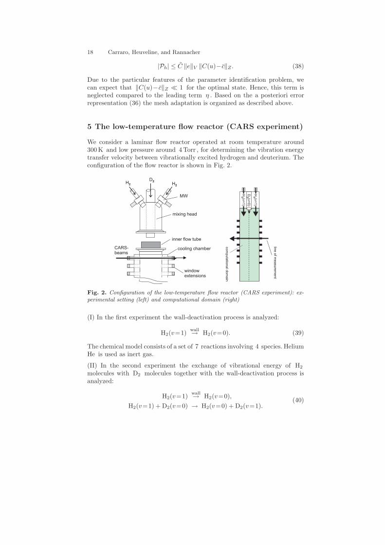
We consider a laminar flow reactor operated at room temperature around300 K and low pressure around 4 Torr , for determining the vibration energytransfer velocity between vibrationally excited hydrogen and deuterium. Theconfiguration of the flow reactor is shown in Fig. 2.

H2 H2

D2

MW

mixing head

inner flow tube

cooling chamber

windowextensions

CARS-beams

H(v

=1

)2

H(v

=1

)2

D2 (v

=0

)

co

mp

uta

tion

al d

om

ain

line

of m

ea

su

rem

en

t

Fig. 2. Configuration of the low-temperature flow reactor (CARS experiment): ex-perimental setting (left) and computational domain (right)

(I) In the first experiment the wall-deactivation process is analyzed:

H2(v=1)wall→ H2(v=0). (39)

The chemical model consists of a set of 7 reactions involving 4 species. HeliumHe is used as inert gas.

(II) In the second experiment the exchange of vibrational energy of H2

molecules with D2 molecules together with the wall-deactivation process isanalyzed:

H2(v=1)wall→ H2(v=0),

H2(v=1) + D2(v=0) → H2(v=0) + D2(v=1).(40)


Vibrationally excited species are treated ‘state-selective’, i.e., each species witha different vibrational level represents a new species with specific thermody-namic and physical properties for which enthalpies and transport coefficientsare changing correspondingly. Initially, close to 200 reaction steps were con-sidered for the present system. However, a sensitivity analysis using a zero-dimensional kinetic algorithm revealed that many of them were of marginalimportance. Therefore, to handle the present full reactive flow problem withreasonable computational work, including the optimization procedure, the re-action mechanism was reduced to the sequence listed in Tables 4 and 5 in theAppendix. The complete chemical model used consists of 29 gas-phase and5 wall reactions involving 8 species. Helium (He) is used as inert gas.

The concentrations of hydrogen and deuterium have been determined bylaser spectroscopical means, particularly a two-color CARS system (CoherentAnti-Stokes Raman Spectroscopy) at several fixed measurement points alongthe reactor axis; for details see the article Hanf/Volpp/Wolfrum [24] in thisvolume. The proportion in mole of the vibrationally excited H2 molecules atthe inlet is 0.5% , the proportion of H atoms is 0.3% , and the rest 99.2% arenot vibrationally excited H2 molecules. With an inflow velocity of 50 m/s theMach number is Ma = 0.018 , such that the low-Mach number approximationis justified. The thermodynamical pressure is set constant to Pth = 5.33 mbar .The assumption about the structure (rotationally symmetric and stationary)of the flow has been checked by an a priori calculation using the flow datarelevant for the reactive flow simulation to be done.

The goal is the determination of the kinetic constants Aj , βj and Eaj

in the temperature range between 180K and 300K from measured CARSsignals which are of the form

J(u) := Ias(p) =

∫

n(r)2f(r − p) dr,

where n(r) is the radial concentration profile of the measured species and pis the location of the beam focus along the beam axis. The accuracy of thesemeasurements is about 20% . The weighting function f(r − p) is equipmentdependent and has to be determined by experimental calibration.

5.1 Results

The wall-deactivation of vibrationally excited hydrogen is reflected by an de-crease of the H2(v = 1)-CARS signal. An optimal adjustment of the sim-ulated CARS signals to the experimental data is reached for a value ofγ = 1.49 · 10−3 for the wall deactivation probabilty for H2(v = 1). The vi-brational energy transfer of hydrogen to deuterium is reflected by an decreaseof the H2(v = 1)-CARS signal and the increase of the D2(v = 1)-CARS sig-nal. An optimal adjustment of the simulated CARS signals to the experi-mental data is reached for a value of k = 1.0 · 10−14 [cm3 molecule−1 s−1]


for the room-temperature rate constant for vibrational energy transfer ofhydrogen to deuterium. This value coincides well with the value k = 1.0 ·10−14 [cm3 molecule−1 s−1] given in Bott et al. [17], and the value k =9.8 · 10−15 [cm3 molecule−1 s−1] given by Pirkle et al. [33], which were ob-tained by other experimental methods. The ‘plug flow’ evaluation yields thesystematically too small value k = 7, 1 · 10−15 [cm3 molecule−1 s−1] . This isexplained by the strong hydrodynamical effects on the distribution of thereactants which are not taken into account by the 0-dimensional analysis.

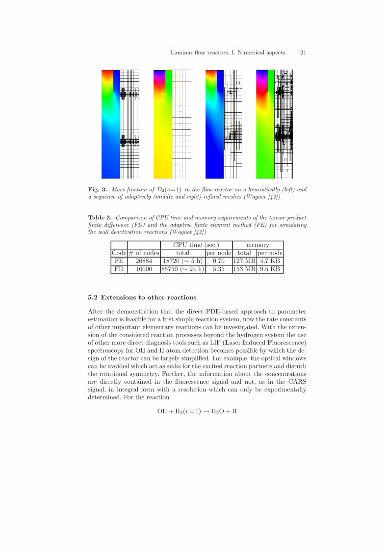
The mass fractions of H2(v=0/1) and D2(v=0/1) obtained by the sim-ulation of the full two-dimensional reactive-flow model are shown in Tables 1.The values obtained on the automatically adapted meshes have a significantlybetter accuracy compared to those on hand-adapted tensor-product meshesand show a monotonic behavior which allows for extrapolation to the limith = 0 . Corresponding species concentrations and adapted meshes are shownin Fig. 3. The increase of performance of the new adaptive finite element codecompared to the earlier (tensor-product) finite difference code is demonstratedin Table 2.

Table 1. Numerical results for the H2 and D2 mass fraction on hand-adapted (left)and on automatically adapted (right) meshes (Waguet [42])

Heuristic refinementL N H2(v=0) H2(v=1)

1 137 0.6556 0.0052942 481 0.7373 0.0066103 1793 0.7962 0.0070964 6913 0.8172 0.0074345 7042 0.8197 0.0074196 7494 0.8240 0.0074737 8492 0.8269 0.0075048 10482 0.8286 0.0075219 15993 0.82853 0.007545

Adaptive refinementL N H2(v=0) H2(v=1)

1 137 0.6556 0.0052942 282 0.7382 0.0060633 619 0.7958 0.0071324 1368 0.8149 0.0073235 3077 0.8257 0.0074576 6800 0.8295 0.0075347 15100 0.8317 0.0075648 33462 0.8328 0.0075879 - - -

Heuristic refinementL N D2(v=0) D2(v=1)

1 137 0.7761 0.0000002 481 0.7422 0.0025413 1793 0.7801 0.0025314 1923 0.7829 0.0027295 2378 0.7851 0.0017136 3380 0.7917 0.0011627 5374 0.7916 0.001436

Adaptive refinementL N D2(v=0) D2(v=1)

1 137 0.7761 0.0000002 244 0.7380 0.0040203 446 0.7450 0.0026004 860 0.7567 0.0020105 1723 0.7806 0.0013906 3427 0.7859 0.0011307 7053 0.7997 0.001090


Fig. 3. Mass fraction of D2(v=1) in the flow reactor on a heuristically (left) anda sequence of adaptively (middle and right) refined meshes (Waguet [42])

Table 2. Comparison of CPU time and memory requirements of the tensor-productfinite difference (FD) and the adaptive finite element method (FE) for simulatingthe wall deactivation reactions (Waguet [42])

CPU time (sec.) memoryCode # of nodes total per node total per nodeFE 26884 18720 (∼ 5 h) 0.70 127 MB 4,7 KBFD 16000 85750 (∼ 24 h) 5.35 153 MB 9.5 KB

5.2 Extensions to other reactions

After the demonstration that the direct PDE-based approach to parameterestimation is feasible for a first simple reaction system, now the rate constantsof other important elementary reactions can be investigated. With the exten-sion of the considered reaction processes beyond the hydrogen system the useof other more direct diagnosis tools such as LIF (Laser Induced Fluorescence)spectroscopy for OH and H atom detection becomes possible by which the de-sign of the reactor can be largely simplified. For example, the optical windowscan be avoided which act as sinks for the excited reaction partners and disturbthe rotational symmetry. Further, the information about the concentrationsare directly contained in the fluorescence signal and not, as in the CARSsignal, in integral form with a resolution which can only be experimentallydetermined. For the reaction

OH + H2(v=1) → H2O + H


the parameter estimation on the basis of the two-dimensional simulationyielded a value of 1.2 · 10−13 [cm3 molecule−1 s−1] for the room-temperaturerate constant, which is in good agreement with the results of full dimensionalquantum scattering calculations performed by Meyer and co-workers [40] (seealso Hanf/Volpp/Wolfrum [24] in this volume).

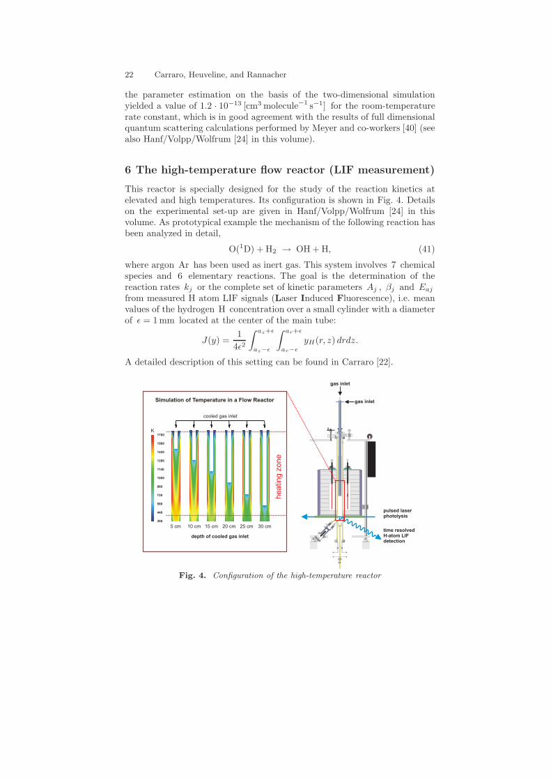
6 The high-temperature flow reactor (LIF measurement)

This reactor is specially designed for the study of the reaction kinetics atelevated and high temperatures. Its configuration is shown in Fig. 4. Detailson the experimental set-up are given in Hanf/Volpp/Wolfrum [24] in thisvolume. As prototypical example the mechanism of the following reaction hasbeen analyzed in detail,

O(1D) + H2 → OH + H, (41)

where argon Ar has been used as inert gas. This system involves 7 chemicalspecies and 6 elementary reactions. The goal is the determination of thereaction rates kj or the complete set of kinetic parameters Aj , βj and Eaj

from measured H atom LIF signals (Laser Induced Fluorescence), i.e. meanvalues of the hydrogen H concentration over a small cylinder with a diameterof ǫ = 1 mm located at the center of the main tube:

J(y) =1

4ǫ2

∫ az+ǫ

az−ǫ

∫ ar+ǫ

ar−ǫ

yH(r, z) drdz.

A detailed description of this setting can be found in Carraro [22].

250mm

1000mm

15mm

44,5/2

25/1

6/1

6/1

6/1

41mm

heating z

one

depth of cooled gas inlet

cooled gas inlet

Simulation of Temperature in a Flow Reactor

pulsed laserphotolysis

gas inlet

gas inlet

time resolvedH-atom LIFdetection

300

440

580

720

860

1000

1140

1280

1420

1560

1700K

5 cm 10 cm 15 cm 20 cm 25 cm 30 cm

Fig. 4. Configuration of the high-temperature reactor


Fig. 5. A time series of temperature plots in the case of non-zero gravity indicatingnonstationary behavior (Carraro [22])

The design of the reactor is largely based on a priori numerical simulation.Especially the question of the achievable temperature in the measurement areais crucial and has been systematically investigated. These computations haveshown that at high temperature and ‘high’ pressure (atmospheric pressure)the inclusion of gravity may result in persisting nonstationary flow behavior;see Fig. 5. This has enforced the restriction of the experiment to low pressureconditions (15 − 50 Torr), such as used in the CARS experiment discussedabove. In order to do controlled measurements in the reactor at high temper-ature and atmospheric pressure the flow needs to be stabilized. An approachto achieve this will be briefly described below.

6.1 Model calibration

The first step in preparing for the simulation of the reactive flow in the reactoris the determination of a complete set of initial and boundary conditions forwhich the model can be expected to be well-posed. For the initial concentra-tion of the species, their partial pressures are calculated from the values oftheir fluxes and the total pressure, and from the partial pressures the initialnumber of molecules per m3 is obtained. The in-flow profiles are calculatedfrom the geometry of the inflow and the fluxes measured experimentally bythe flux controllers. The out-flow boundary conditions, the no-slip conditionat rigid walls and the symmetry condition along the cylinder axis are imposedas usual. Only the temperature boundary condition at the outer wall is notso clearly defined. This is a typical difficulty for the simulation of real-lifeexperiments. The reactor is heated at the exterior wall in order to achievethe desired high temperature in the interior. However, due to constructionalconstraints the exact temperature distribution along the outer wall cannot bedirectly measured and is actually nonuniform due to the cold inflow at the


upper inlets. The only information available is the temperature profile alongthe inner reactor axis which is obtained from thermo-sensor measurements.This is taken as input data for the implicit determination of the unknown tem-perature boundary data by a parameter estimation process (see the geometrydescription in Fig. 6).

y5

y6

y7

y8

y2

y3

y4

y1

N2OH2 ArAr

mea

sure

d te

mpe

ratu

re

tem

pera

ture

’s b

ound

ary

cond

itio

n

Laser

Fig. 6. Geometry sketch of the experiment for the calibration of the temperatureboundary condition (left), computed temperature with 780 K in the measurementarea (middle), and an adapted mesh for the flow simulation (right) (Carraro [22])

- The temperature profile along the wall is assumed as a piecewise linearfunction described by 6 parameters, the temperature values at the posi-tions y2, . . . , y7 , to be determined.

- Input data for the parameter estimation are measured profiles Tmeas ofthe temperature along the symmetry axis.

- The parameters are determined by minimizing the least squares functional

F (T ) =1

2

∫

Γsym

|Tsim − Tmeas|2 dz

for the measured and computed temperature profile along the symmetryaxis subject to the flow equations.

Such a ‘model calibration’ has to be done within each measurement cycle inthe reactor. The result of this calibration of temperature boundary conditionsfor an experiment with 580K in the heating zone is shown in Fig. 7.


0

50

100

150

200

250

300

350

-20 -10 0 10 20 30 40 50 60

Tem

pera

ture

[C]

Position [cm]

Calibration of the temperature at the boundary

Experimental MeasurementsBoundary Temp.: result of param. estim.

Simulated Temperature

Fig. 7. Temperature profiles along the symmetry axis in the calibration of boundaryconditions (Carraro [22])

Experimentally the reaction starts with the photodissociation of N2O inN2 and O(1D) produced by an ArF (193 nm) excimer laser. The detectionof H atoms is done by the laser-induced fluorescence (LIF) technique. Inthe numerical case the photodissociation has been simulated by an ignitionmechanism and the detection is an integration in the measurement volumeof the mass fraction of the H atoms. The LIF signal is proportional to thenumber of H atoms that are in the measurement volume, so to compare thetwo signals (the experimental and the numerical one), we have to consider anadditional parameter, that is the unknown scaling factor of the LIF signal.

Fig. 8 shows zooms into the measurement area before and after ignition.The depicted distributions of H2 and N2O indicate that the inflow from theside tubes at the optical zone does not much affect the concentration at themeasurement point. Fig. 9 shows H mass fractions at different times (timestep 100 ns ) during the reaction process. Computed distributions of severalof the relevant quantities are shown in Fig. 10.


Fig. 8. H2 (left) and N2O distribution before ignition (left/middle) and duringignition (right) (Carraro [22])

Fig. 9. Computed H mass fractions at different times (time step 100 ns ) duringthe reaction process (Carraro [22])

Fig. 10. Computed H2, temperature, axial-velocity component, and N2O (from leftto right) in the stationary solution under zero gravity (Carraro [22])


6.2 Flow stabilization

At high temperature and atmospheric pressure the flow in the flow reactorshows fully nonstationary behavior caused by temperature-gradient drivenconvection. But for a reliable LIF measurement we need stationary flow con-ditions in the measurement zone. This can be achieved by artificial stabiliza-tion of the flow by optimal control techniques. The idea is to modulate theboundary heating in such a way that at least in the measurement zone Ωmeas

the nonstationary behavior is suppressed. To this end, we try to minimize thecost functional

J(u) =K

2

∫ T

0

‖∂tv(t)‖2Ωmeas

+ ‖∂tT (t)‖2Ωmeas

dt + ‘Regularization’,

where u = v, p, T, y is determined by the flow model (12) - (16), and q(t)is the prescribed time-dependent exterior heat distribution which is used tocontrol the dynamics of the flow behavior, T (·, t)|∂Ω = q(·, t), t ∈ [0, T ] . Theapplication of this approach to the high-temperature flow reactor is subjectof current work. It is expected that in this way the LIF measurements can beextended to atmospheric pressure.

6.3 Parameter estimation

Due to the limitations imposed by the flow conditions discussed above, theLIF measurements in the high-temperature flow reactor had to be restrictedto low pressure, 15 − 50 Torr, and intermediate temperature, 300 − 800 K .The quantity to be determined is the reaction rate

k(T ) = A( T

300K

)β

exp(

− Ea

RT

)

, (42)

of the reaction of interest, O(1D) + H2 → OH + H , while the rates of allthe other participating elementary reactions are supposed to be known withsufficient accuracy over the full temperature range. Since the experiment iscarried out for fixed known temperature and the activation energy Ea israther small the reaction rate k(T ) can directly be determined from measuredvalues of the concentration of hydrogen H at different temperature.

The experiments have been repeated with different initial conditions,changing the ratio of the concentration of the species at the inflow: H2 , N2Oand Ar . The number of molecules of each species is determined by the flowsin the cooled gas inlet and in the bathgas inlet, determined by flow regula-tors. In all cases the concentration of H2 can be considered in excess so thatduring the reaction it can be regarded as almost constant for the calculationof the reaction rate. For the determination of the reaction rate 6 differentsetups have been used, obtained by varying the inflow regulator of H2 from5 % to 50 % . From these 6 data sets a pseudo first order reaction rate canbe estimated and from this the ‘true’ reaction rate, for a given temperature.


With this technique the reaction rate has been determined ‘experimen-tally’; for more details, we refer to the article Hanf/Volpp/Wolfrum [24] inthis volume. For the numerical estimation of the reaction rates, we just needone experimental curve for one of the values of the initial concentration. Wedemonstrate this in the case of T = 300 K comparing the numerical resultsin two extreme cases: the first with the flow regulator for H2 at 50 % of themaximum value and the second at 5 % . The measured values shortly afterthe ignition time are most significant for the reaction parameter, while laterthe measured values are rather scattered.

Experiment 1: T = 300 K and 50% H2-inflow concentration

- Pressure p = 1866 Pa (14 Torr) .- Inflow mass fraction yH2

= 0.016 , yN2O = 0.0236 .- Inflow velocity in the main tube v = 0.86 m/s and in the optical cooling

system v = 0.55 m/s .

The parameter identification process determines the desired reaction rate as

k = 1.0 · 10−10 [cm3 molecule−1 s−1].

Fig. 11 gives the comparison between the corresponding computed and mea-sured H concentrations. The two curves for the parameter values k =0.9 · 10−10 [cm3 molecule−1 s−1] and k = 1.1 · 10−10 [cm3 molecule−1 s−1] areshown to demonstrate the sensitivity of the result with respect the value ofthe reaction rate.

-0.02

0

0.02

0.04

0.06

0.08

0.1

0.12

0.14

0.16

0.18

-400 -200 0 200 400 600 800

LIF

Sig

nal [

-]

Time [ns]

H Concentration: Simulation vs Experiment, 50% H2, 14 Torr, 300 K

k=1e-10

k=0.9e-10

k=1.1e-10

Experiment

Fig. 11. Computed H concentrations using estimated parameters versus experi-mental data ( H atom LIF signal) at room temperature 300 K (Carraro [22])



- Pressure p = 1866 Pa (14 Torr) .- Inflow mass fraction yH2




k = 1.0 · 10−10 [cm3 molecule−1 s−1].

Fig. 12 gives the comparison between the corresponding computed and mea-sured H concentrations.


- Pressure p = 5866 Pa (43.8 Torr) .- Inflow mass fraction yH2




k = 1.5 · 10−10 [cm3 molecule−1 s−1].

Fig. 13 shows the comparison between the corresponding computed and mea-sured H concentrations.

0

0.002

0.004

0.006

0.008

0.01

0.012

0.014

0.016

-400 -200 0 200 400 600 800

LIF

Sig

nal [

-]

Time [ns]

H Concentration: Simulation vs Experiment, 5% H2, 14 Torr, 300 K

Experiment

k=1.0e-10

Fig. 12. Computed H concentrations using estimated parameters versus experi-mental data ( H atom LIF signal) at room temperature 300 K (Carraro [22])


-0.02

0

0.02

0.04

0.06

0.08

0.1

0.12

0.14

0.16

0.18

-300 -200 -100 0 100 200 300 400 500

LIF

Sig

nal [

-]

Time [ns]

H Concentration: Simulation vs Experiment, 50% H2, 43.8 Torr, 780 K

k=1.5e-10

Experiment

Fig. 13. Computed H concentrations using estimated parameters versus experimen-tal data (H atom LIF signal) at higher temperature 780 K (Carraro [22])

7 A step towards optimal experimental design

For the high-temperature reactor also the question of systematic experimentoptimization (‘optimal experimental design’) has been considered. The vari-ances of parameter estimates and prediction depend upon this design. Un-necessarily large variances and imprecise predictions resulting from a poorlydesigned experiment largely wastes resources. Hence, the goal is to choose themodel parameters, e.g., the inflow velocity and the position of the inner pipe,in such a way that the sensitivity of the reaction parameter to be determinedis maximal. The proposed approach takes also into account the statisticalproperties of a random error in the measurements.

The parameter estimation procedure uses a merit-function of least-squarestype which is particularly convenient for its numerical solution. We assume aphysical model which is described by means of partial differential equationsdepending on a finite number of parameters q := (q1, · · · , qM ) ∈ Q ⊂ R

M . Intheir weak form the corresponding state equations can be formulated as

A(u, q)(ϕ) = 0 ∀ϕ ∈ V, (43)

where u is the state variable defined in an appropriate Hilbert space V . Asbefore, the semi-linear form A(·, ·)(·) which is defined on the Hilbert space(V × Q) × V may be nonlinear only with regard to its first two arguments,the state variable u and the control parameter q. We assume that each q ∈ Qdefines a unique solution uq ∈ V of the problem (43). Further, let the experi-

mental set-up be characterized by a set D ⊂ RN of so-called experiment ex-


planatory variables ξ = (ξ1, . . . , ξN ) . Then, in order to determine the correctparameters q∗ describing the considered physical problem, we suppose thatfor each parameter set ξ ∈ D and any given state u , we have measurementsof N observable quantities denoted by c(ξ, u) ∈ R

N . The measurements ob-tained by means of the experiment explanatory variable ξ which describes theexperimental design are denoted by c(ξ), where c : D → R

N . As depicted inFig. 14, the measurements are subject to random errors ǫ = (ǫ1, · · · , ǫN ) andc(ξ) should therefore be understood as an N -dimensional random variable.For simplifying notation, in the following we assume that N = N

One crucial assumption is that the underlying model is an exact descriptionof the physical process considered, i.e., modelling errors are negligibly smallcompared to measurement errors, and we have

c(ξ) = c(ξ, u) + ǫ. (44)

Further, the statistical assumptions are made that the random errors ǫ havea Gauß distribution,

var(ǫi) = σ2, (45)

and posses covariance and expectation value zero,

cov(ǫi, ǫj) = 0, E(ǫi) = 0. (46)

The formulation of the parameter identification problem as a least-squaresproblem is consistent with these statistical assumptions.

-

-

-

-

-

-

6 6 6,

,, @@@

ξ1

ξ2

ξN

c1

c2

cN

ǫ1 ǫ2 ǫN

ERRORS

INPUTS / RESPONSES

Fig. 14. Schematic representation of an experiment: The experiment explanatoryvariables (ξ1, · · · , ξ

N) describe the current experimental design. The measurement re-

sponses (c1, · · · , cN ) are random variables. Their dependence on the experiment ex-planatory variables (ξ1, · · · , ξ

N) is blurred by the uncontrollable errors (ǫ1, · · · , ǫN ).

As an example of this setting, we consider the case of point measurementsof the state variable u at certain points xi in the region Ω . Accordingly, weset D := Ωobs = xi, i = 1, . . . , xN ∈ R

N and


c(xi, u) :=1

|Bǫ(xi)|

∫

Bǫ(xi)

ω(|xi − x|)uq(x) dx,

where Bǫ(xi) ⊂ Rd denotes the ball centered in xi with radius ǫ > 0 ,

and ω(·) is an adequate weighting function. If well defined in the consideredfunctional analytical set-up, the mapping c(·, ·) could even reduce to sharppoint evaluations (Dirac functionals) c(xi, u) := uq(xi), i = 1, . . . , N .

The parameter identification problem aims at solving the following prob-lem for a given ξ ∈ H :

12‖C(u, ξ) − c(ξ)‖2

Z →q∈Q min,

A(u, q)(ϕ) = 0 ∀ϕ ∈ V.(47)

Now, the question is to determine ‘optimal’ explanatory variables ξ in order toimprove statistically the results of the parameter identification problem (47).This means that the covariance matrix coV := σ−2(G∗G)−1 of the parametersshould be optimized. Common optimization criteria are the maximization of

Φ(coV ) =

det(coV ) (determinant: Criterion D),

tr(coV ) (trace: Criterion A),

σ(coV ) (spectral radius: Criterion E),

with respect to the design parameter ξ ∈ D of the model, the mentionedposition of the inner pipe or the inflow velocity in the present case,

Φ(coV (ξ)) →ξ∈D min . (48)

7.1 Numerical experiment

To illustrate the principles of our approach to optimal experimental designin the context of the chemical flow reactor, as a model case, we consider thereaction between two chemical species, where the balance equation for themass fraction u of one species is our model,

µ(∇u,∇ϕ) + (b · ∇u, ϕ) = (mω,ϕ) in Ω, u = 0 on ∂Ω. (49)

The domain is the unit square Ω = (0, 1) × (0, 1) , and the mass fraction vof the other species is obtained by v := 1 − u . Here, µ is the correspondingdiffusion coefficient, b the velocity of the base flow, m the molecular mass,and ω the molar production rate of the species. The latter has the form ω =kc , with k the reaction rate and c the species concentration. An Arrheniuslaw is assumed for k ,

k = A( T

300K

)β

exp(

− Ea

RT

)

, (50)


where the factor A , the temperature T , the activation energy Ea , and thegas constant R are given parameters. We want to identify the rate constant kand the diffusion coefficient µ from given ‘measurement’ data of the solution.To this end, we assume 3 point measurements of u at 3 positions in the flowdomain. The first two measurement points are the same for all consideredcases, while the third measurement is determined as the result of the optimalexperimental design using the three different optimality criteria (D), (A) and(E), described above. In one case the measurement is taken at a position whichis not an optimal design point. To each measurement we have added the sameerror, that is given by the 10% of the maximum of the value u in the domain.The fixed system parameters are

b = (1.5, 0.3)T , xmeas1 = (0.4, 0.3)T , xmeas

2 = (0.6, 0.5)T ,

and the measurement error is ǫ = 10% umax = 0.016 .The results of the design optimization are shown in Table 3: the values of

the estimated parameters for all criteria D, A, and E, the values of the erroradded and the dimensions of the 95% confidence regions, that are the area ofthe ellipses (minimized by the D criterion), the length of the axes (minimizedby the E criterion) and the sum of the lengths of the axes (minimized by the Acriterion). The least squares functional is the distance between the measuredvalues of umeas and the approximated ones by the finite element model,

F = 12‖umeas − u‖2.

Fig. 17 shows corresponding confidence regions (ellipses). Obviously the con-fidence regions in the “non OED” case are much larger than in the othercases.

0 0.02 0.04 0.06 0.08 0.1 0.12 0.14 0.16 0.18

Solution

0 0.2 0.4 0.6 0.8 1

x 0

0.2 0.4

0.6 0.8 1

y

0 0.02 0.04 0.06 0.08

0.1 0.12 0.14 0.16 0.18

u

0 0.02 0.04 0.06 0.08 0.1 0.12 0.14 0.16 0.18

Solution

0 0.2 0.4 0.6 0.8 1

x 0

0.2 0.4

0.6 0.8 1

y

0 0.02 0.04 0.06 0.08

0.1 0.12 0.14 0.16 0.18

u

Fig. 15. Solution u for the nominal parameters (Carraro [22])


Table 3. Optimization results and 95%-confidence region (Carraro [22])

no OED D A E True Value

Meas 3 (0.9,0.5) (0.12,0.27) (0.11,0.2) (0.11,0.2) -Param 1: µ 0.236819 0.194105 0.184985 0.184985 0.2Param 2: k 8817.56 11654.1 12215.3 12215.3 15000Area Ellipse 1.0220e+04 2586.0 2655.6 2655.6 -Min Axis 0.068075 0.051487 0.054365 0.054365 -Max Axis 4.7788e+04 1.5988e+04 1.5549e+04 1.5549e+04 -Sum Axes 4.7788e+04 1.5988e+04 1.5549e+04 1.5549e+04 -

2e+11 4e+11 6e+11 8e+11 1e+12 1.2e+12 1.4e+12 1.6e+12 1.8e+12 2e+12 2.2e+12

A Criterion

0.1 0.2 0.3 0.4 0.5 0.6 0.7 0.8 0.9x 0.1

0.2 0.3

0.4 0.5

0.6 0.7

0.8 0.9

y

2e+11 4e+11 6e+11 8e+11 1e+12

1.2e+12 1.4e+12 1.6e+12 1.8e+12

2e+12 2.2e+12

Criterion

2e+11 4e+11 6e+11 8e+11 1e+12 1.2e+12 1.4e+12 1.6e+12 1.8e+12 2e+12 2.2e+12

A Criterion

0.1 0.2 0.3 0.4 0.5 0.6 0.7 0.8 0.9x 0.1

0.2 0.3

0.4 0.5

0.6 0.7

0.8 0.9

y

2e+11 4e+11 6e+11 8e+11 1e+12

1.2e+12 1.4e+12 1.6e+12 1.8e+12

2e+12 2.2e+12

Criterion

0 1e+12 2e+12 3e+12 4e+12 5e+12 6e+12 7e+12 8e+12 9e+12 1e+13 1.1e+13

D Criterion

0.1 0.2 0.3 0.4 0.5 0.6 0.7 0.8 0.9x 0.1

0.2 0.3

0.4 0.5

0.6 0.7

0.8 0.9

y

0 1e+12 2e+12 3e+12 4e+12 5e+12 6e+12 7e+12 8e+12 9e+12 1e+13

1.1e+13

Criterion

0 1e+12 2e+12 3e+12 4e+12 5e+12 6e+12 7e+12 8e+12 9e+12 1e+13 1.1e+13

D Criterion

0.1 0.2 0.3 0.4 0.5 0.6 0.7 0.8 0.9x 0.1

0.2 0.3

0.4 0.5

0.6 0.7

0.8 0.9

y

0 1e+12 2e+12 3e+12 4e+12 5e+12 6e+12 7e+12 8e+12 9e+12 1e+13

1.1e+13

Criterion

Fig. 16. Determinant (left) and trace (right) of the covariance matrix (Carraro [22])

-40000

-30000

-20000

-10000

0

10000

20000

30000

40000

50000

60000

-0.6 -0.4 -0.2 0 0.2 0.4 0.6 0.8 1

γ

α

95% Confidence Region

No Opt. Exp. Design

Meas 3 = [0.9,0.5]

A, E Criterion

Meas 3 = [0.11,0.2]

D Criterion

Meas 3 = [0.12,0.27]

D Criterion

A Criterion

E Criterion

No Criterion

-40000

-30000

-20000

-10000

0

10000

20000

30000

40000

50000

60000

-0.6 -0.4 -0.2 0 0.2 0.4 0.6 0.8 1

γ

α

95% Confidence Region

No Opt. Exp. Design

Meas 3 = [0.9,0.5]

A, E Criterion

Meas 3 = [0.11,0.2]

D Criterion

Meas 3 = [0.12,0.27]

D Criterion

A Criterion

E Criterion

No Criterion

Fig. 17. Confidence regions for criteria (A), (D) and “non OED” (Carraro [22])


8 Conclusion and outlook

In this project it has been demonstrated that experiments combined with nu-merical evaluation can be an effective tool for determining kinetic parametersof elementary reactions in flow reactors in a wide temperature range. Theapproach is currently extended into various directions:

• Other reaction mechanisms: After the setting up of the high-temperatureflow-reactor system and its first successful application in kinetics studiesof the O(1D)+H2 reaction(41), more complex systems, such as NH+NO ,NH + O2 , NH2 + NO , CH2 + NO , and CH + N2 which have multiplereaction product channels can be studied over an extended range of tem-perature.

• Optimal experimental design: The approach to optimal experimental de-sign described in this article has to be developed further in order to beapplied to the high-temperature reactor as well as to other types of flowreactors which contain more control parameters.

• Optimal experimental control: In the case of higher, i.e., atmospheric pres-sure, the flow in the reactor is nonstationary due to temperature-drivenconvection. It should be possible to stabilize this flow by nonstationarymodulation of the wall heating such that it becomes (almost) stationaryat least in the measurement area. This would allow the extension of thekinetics studies to atmospheric pressure conditions.

9 Appendix

In the following, we list the detailed reaction systems used in the simulationsof the flow reactors described in this article.

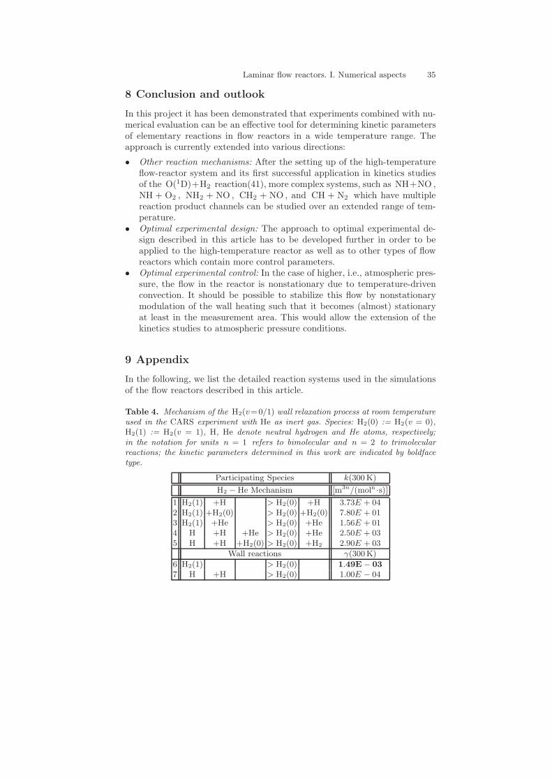
Table 4. Mechanism of the H2(v=0/1) wall relaxation process at room temperatureused in the CARS experiment with He as inert gas. Species: H2(0) := H2(v = 0),H2(1) := H2(v = 1), H, He denote neutral hydrogen and He atoms, respectively;in the notation for units n = 1 refers to bimolecular and n = 2 to trimolecularreactions; the kinetic parameters determined in this work are indicated by boldfacetype.

Participating Species k(300 K)

H2 − He Mechanism [m3n/(moln ·s)]

1 H2(1) +H > H2(0) +H 3.73E + 042 H2(1) +H2(0) > H2(0) +H2(0) 7.80E + 013 H2(1) +He > H2(0) +He 1.56E + 014 H +H +He > H2(0) +He 2.50E + 035 H +H +H2(0) > H2(0) +H2 2.90E + 03

Wall reactions γ(300K)

6 H2(1) > H2(0) 1.49E − 03

7 H +H > H2(0) 1.00E − 04


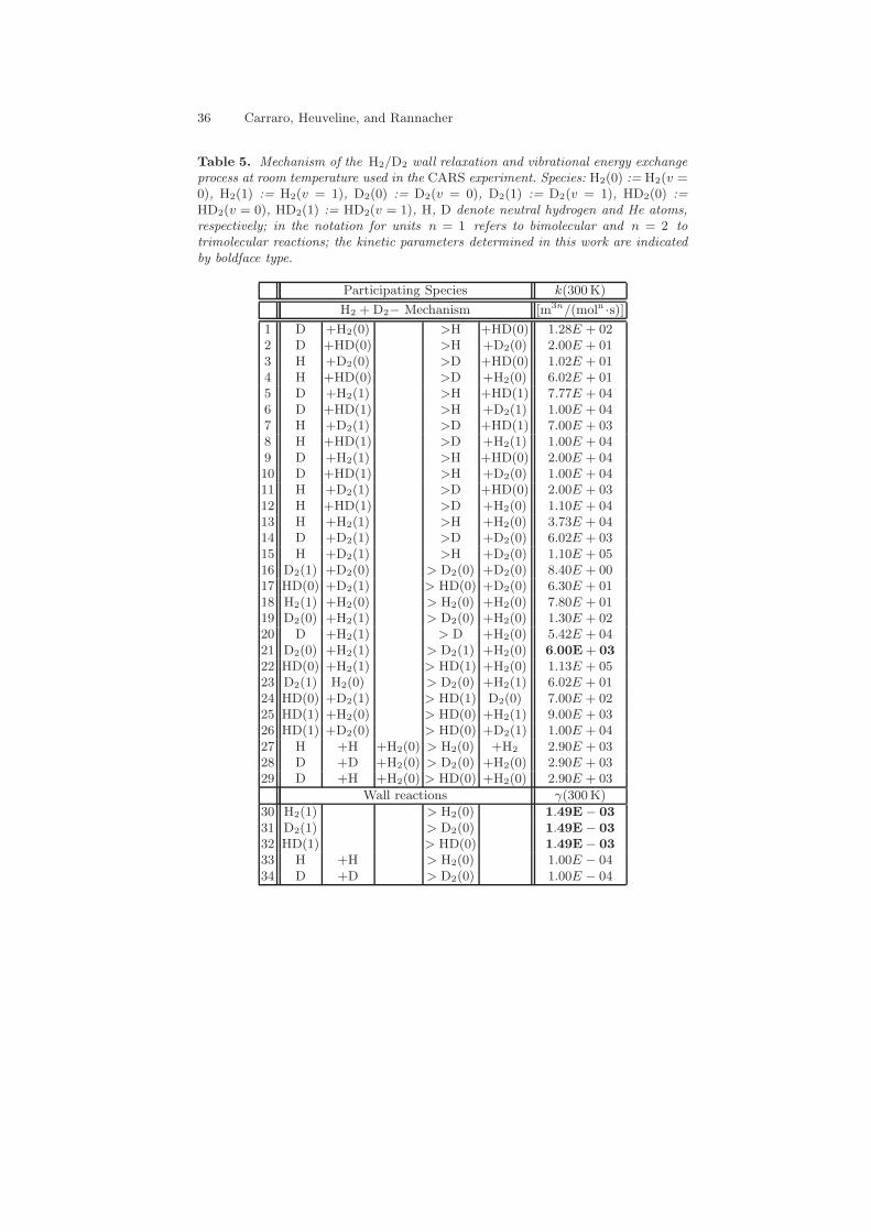
Table 5. Mechanism of the H2/D2 wall relaxation and vibrational energy exchangeprocess at room temperature used in the CARS experiment. Species: H2(0) := H2(v =0), H2(1) := H2(v = 1), D2(0) := D2(v = 0), D2(1) := D2(v = 1), HD2(0) :=HD2(v = 0), HD2(1) := HD2(v = 1), H, D denote neutral hydrogen and He atoms,respectively; in the notation for units n = 1 refers to bimolecular and n = 2 totrimolecular reactions; the kinetic parameters determined in this work are indicatedby boldface type.

Participating Species k(300 K)

H2 + D2− Mechanism [m3n/(moln ·s)]

1 D +H2(0) >H +HD(0) 1.28E + 022 D +HD(0) >H +D2(0) 2.00E + 013 H +D2(0) >D +HD(0) 1.02E + 014 H +HD(0) >D +H2(0) 6.02E + 015 D +H2(1) >H +HD(1) 7.77E + 046 D +HD(1) >H +D2(1) 1.00E + 047 H +D2(1) >D +HD(1) 7.00E + 038 H +HD(1) >D +H2(1) 1.00E + 049 D +H2(1) >H +HD(0) 2.00E + 0410 D +HD(1) >H +D2(0) 1.00E + 0411 H +D2(1) >D +HD(0) 2.00E + 0312 H +HD(1) >D +H2(0) 1.10E + 0413 H +H2(1) >H +H2(0) 3.73E + 0414 D +D2(1) >D +D2(0) 6.02E + 0315 H +D2(1) >H +D2(0) 1.10E + 0516 D2(1) +D2(0) > D2(0) +D2(0) 8.40E + 0017 HD(0) +D2(1) > HD(0) +D2(0) 6.30E + 0118 H2(1) +H2(0) > H2(0) +H2(0) 7.80E + 0119 D2(0) +H2(1) > D2(0) +H2(0) 1.30E + 0220 D +H2(1) > D +H2(0) 5.42E + 0421 D2(0) +H2(1) > D2(1) +H2(0) 6.00E + 03

22 HD(0) +H2(1) > HD(1) +H2(0) 1.13E + 0523 D2(1) H2(0) > D2(0) +H2(1) 6.02E + 0124 HD(0) +D2(1) > HD(1) D2(0) 7.00E + 0225 HD(1) +H2(0) > HD(0) +H2(1) 9.00E + 0326 HD(1) +D2(0) > HD(0) +D2(1) 1.00E + 0427 H +H +H2(0) > H2(0) +H2 2.90E + 0328 D +D +H2(0) > D2(0) +H2(0) 2.90E + 0329 D +H +H2(0) > HD(0) +H2(0) 2.90E + 03

Wall reactions γ(300 K)

30 H2(1) > H2(0) 1.49E − 03

31 D2(1) > D2(0) 1.49E − 03

32 HD(1) > HD(0) 1.49E − 03

33 H +H > H2(0) 1.00E − 0434 D +D > D2(0) 1.00E − 04


Table 6. Mechanism of the O(1D) + H2 reaction with Ar as inert gas used inthe high-temperature LIF experiment: primary, secondary and tertiary reactions; theabbreviations O := O(3P ) and O∗ := O(1D) are used; the = sign means that thebackward reaction is included; in the notation for units n = 1 refers to bimolecularand n = 2 to trimolecular reactions; the kinetic parameters determined in this workare indicated by boldface type.

Participating Species A β Ea

[m3n/(moln ·s)] [kJ/mol]

1 O∗ +Ar >O +Ar 3.011E + 05 0.0 0.000

Primary and secondary reactions (48 species)

2 O∗ +H2 >OH +H 6.020E + 06 1.96 −5.7503 O∗ +N2O >O +N2O 6.022E + 05 0.0 0.0004 O∗ +N2O >NO +NO 4.336E + 07 0.0 0.0005 O∗ +N2O >N2 +O2 2.650E + 07 0.0 0.0006 N2O +H2 >H2O +N2 3.451E + 06 0.5 0.0007 OH +N2O >N2 +HO2 8.431E + 06 0.0 41.5728 OH +N2O =HNO +NO 6.082E + 00 4.3 104.7629 OH +H2 >H +H2O 9.334E + 05 1.6 13.80210 O +N2O =NO +NO 6.624E + 07 0.0 111.41411 O +N2O >N2 +O2 1.018E + 08 0.0 117.23412 O +H2 >H +OH 2.072E + 05 2.7 26.27413 NO +N2O >NO2 +N2 1.728E + 05 2.2 193.72714 NO +O∗ >O +NO 2.409E + 07 0.0 0.00015 NO +O∗ >N +O2 5.119E + 07 0.0 0.00016 NO +H2 =HNO +H 1.078E + 06 2.3 212.01917 H2O +O∗ >OH +OH 1.319E + 08 0.0 0.00018 H +N2O >N2 +OH 9.635E + 07 0.0 63.19019 H +N2O =NH +NO 3.029E + 11 −2.2 155.481

Tertiary reactions (16 species)

20 OH +OH >H2O +O 3.101E + 04 2.4 −8.81321 O +OH =H +O2 2.608E + 07 −0.5 0.24922 O +O +Ar >O2 +Ar 4.098E + 01 0.0 −4.40723 NO +OH =HNO2 1.499E + 06 −0.1 3.01824 NO +OH +Ar =HNO2 +Ar 3.130E + 05 −2.5 0.28325 NO +O =N +O2 5.378E + 05 1.0 162.13226 NO +O =NO2 1.813E + 07 0.3 0.00027 NO +O +Ar > NO2 +Ar 2.430E + 04 −1.4 0.00028 NO +NO >N2 +O2 3.071E + 06 0.5 253.59129 H2O +OH = H2O +OH 1.391E + 05 0.0 17.46030 H2O +O >OH +OH 7.528E + 06 1.3 71.50431 H +OH > H2O 1.620E + 08 0.0 0.62432 H +OH +Ar >H2O +Ar 9.393E + 04 −2.0 0.00033 H +OH >O +H2 4.131E + 04 2.8 16.21334 H +O >O +H 1.581E + 04 −1.0 0.00035 H +NO =N +OH 2.168E + 08 0.0 207.03036 H +NO =O +NH 5.600E + 08 −0.1 292.03037 H +NO =HNO 1.469E + 08 −0.4 0.00038 H +NO +Ar =HNO +Ar 4.859E + 04 −1.3 3.07639 H +H2O >OH +H2 4.107E + 06 1.6 80.81740 H +H +Ar >H2 +Ar 2.190E + 04 −1.0 0.000


References

1. J. P. D. Abbatt, K. L. Demerjian, and J. G. Anderson: A new approach tofree-radical kinetics: radially and axially resolved high-pressure discharge flowwith results for OH+(C2H6, C3H8, n-C4H10, n-C5H12)→ products at 297 K,J. Chem. Phys. 94, 4566-4575 (1990).

2. J. Arnold, T. Bouche, T. Dreier, J. Wichmann, J. Wolfrum: CARS studies onthe heterogeneous relaxation of vibrationally excited hydrogen and deuterium,Chem. Phys. Lett. 203, 283 (1993).

3. W. Bangerth and R. Rannacher: Adaptive Finite Element Methods for Differen-tial Equations, Lectures in Mathematics, ETH Zurich, Birkhauser, Basel 2003.

4. R. Becker: An optimal control approach to a posteriori error estimation for fi-nite element discretizations of the Navier-Stokes equations, East-West J. Nu-mer. Math. 8, 257-274 (2000).

5. R. Becker: Adaptive Finite Elements for Optimal Control Problems, Habilita-tionsschrift, Institut fur Angewandte Mathematik, Universitat Heidelberg, 2001.

6. R. Becker, M. Braack, R .Rannacher, and C. Waguet: Fast and reliable solutionsof the Navier-Stokes equations including chemistry, Comput. Visual. Sci. 2, 107–122 (1999).

7. R. Becker, M. Braack, and B. Vexler: Numerical parameter estimation for chem-ical models in multidimensional reactive flows, to appear in Combustion Theoryand Modelling 8, 661–682 (2004).

8. R. Becker, M. Braack, and B. Vexler: Parameter identification for chemical mod-els in combustion problems, to appear in Appl. Numer. Math. (2004).

9. R. Becker, V. Heuveline, and R. Rannacher: An optimal control approach toadaptivity in computational fluid mechanics, Int. J. Numer. Meth. Fluids. 40,105-120 (2002).

10. R. Becker, G. Kanschat, F.-T. Suttmeier: DEAL, Differential Equations Anal-ysis Library, Release 1.0, Technical Report, University of Heidelberg 1995.

11. R. Becker, H. Kapp, and R. Rannacher: Adaptive finite element methods foroptimal control of partial differential equations: basic concepts, SIAM J. Opti-mization Control 39, 113-132 (2000).

12. R. Becker, H. Kapp, D. Meidner, R. Rannacher, and B. Vexler: Adaptive finiteelement methods for PDE-constrained optimal control problems, Reactive Flows,Diffusion and Transport, (R. Rannacher et al., eds), Springer, Berlin-Heidelberg,2005.

13. R. Becker and R. Rannacher: Weighted a-posteriori error estimates in FE meth-ods, Lecture ENUMATH-95, Paris, Sept. 18-22, 1995, in: Proc. ENUMATH-97,Heidelberg, Sept. 28 - Oct.3, 1997 (H.G. Bock, et al., eds), pp. 621-637, WorldScientific Publ., Singapore, 1998.

14. R. Becker and R. Rannacher: An optimal control approach to error estimationand mesh adaptation in finite element methods, Acta Numerica 2000 (A. Iserles,ed.), pp. 1-102, Cambridge University Press, 2001.

15. R. Becker and B. Vexler: A Posteriori error estimation for finite elementdiscretization of parameter identification problems, Numer. Math. 96, 435–459(2004).

16. G. D. Billing, R. E. Kolesnik: Chem. Phys. Lett. 215, 571 (1993).17. J. F. Bott: Vibrational energy exchange between H2(v=1) and D2, N2, HCl, and

CO2, J. Chem. Phys. 65, 3921 (1976).


18. M. Braack: An Adaptive Finite Element Method for Combustion Problems, Dis-sertation, Institut fur Angewandte Mathematik, Universitat Heidelberg, 1998.

19. M. Braack and T. Richter: Solving multidimensional reactive flow problems withadaptive finite elements, Reactive Flows, Diffusion and Transport, (R. Rannacheret al., eds), Springer, Berlin-Heidelberg, 2005.

20. M. Braack and R. Rannacher: Adaptive finite element methods for low-mach-number flows with chemical reactions, 30th Computational Fluid Dynamics(H. Deconinck, ed.), Volume 1999-03 of Lecture Series von Karman Institutefor Fluid Dynamics, 1999.

21. M. Cacciatore and G. D. Billing: State-to-state vibration-translation andvibration-vibration rate constants in H2-H2 and HD-HD collisions, J. Phys.Chem. 96, 217 (1992).

22. T. Carraro: Parameter estimation and experimental design in flow reactors, Dis-sertation, Institut fur Angewandte Mathematik, Universitat Heidelberg, 2005.

23. A. Hanf: Konstruktion eines Hochtemperaturstrmungsreaktors und Unter-suchung der Reaktion O(1D)+H2 → OH +H bei hohen Temperaturen, Dis-sertation, Physikalisch-Chemisches Institut, Universitat Heidelberg, 2005.

24. A. Hanf, H.-R. Volpp, and J. Wolfrum: Determination of kinetic parameters inlaminar flow reactors. II. Experimental aspects, Reactive Flows, Diffusion andTransport, (R. Rannacher et al., eds), Springer, Berlin-Heidelberg, 2005.

25. F.-K. Hebeker and R. Rannacher: An adaptive finite element method for un-steady convection-dominated flows with stiff source terms, SIAM J. Sci. Comput.21, 799–818 (1999).

26. V. Heuveline: HiFlow: A finite element solver package, http://www.hiflow.de/.27. V. Heuveline and A. Walther: Online checkpointing for adjoint computation in

PDEs: Application to goal-oriented adaptivity and flow control, Preprint, Com-puter Center, University of Karlsruhe, accepted for publication.

28. P. Houston, R. Rannacher, and E. Suli: A posteriori error analysis for sta-bilized finite element approximations of transport problems, Comput. MethodsAppl. Mech. Engrg 190, 1483–1508 (2000).

29. F. Kaufman: Progress in Reaction Kinetics, Vol. 1, Pergamon Press, 1961.30. R. J. Kee, F. M. Rupley, and J. A. Miller: The chemkin thermodynamical data

base, Report SAND87-8215.UC4, Sandia National Laboratories, USA, 198731. J. Nocedal and S. J. Wright: Numerical Optimization, Springer Series in Oper-

ations Research, Springer, New York, 1999.32. R. J. Pirkle and T. A. Cool: Vibrational energy transfer for H2-D2 and H2-HCl

mixtures from 220-450 K, Chem. Phys. Lett. 42, 58 (1976).33. R. V. Poirier and R. W. Carr, Jr.: The Use of tubular flow reactors for kinetic

studies over extended pressure ranges, J. Phys. Chem. 75, 1593-1601 (1971).34. R. Rannacher: Adaptive finite element discretization of optimization problems,

Proc. Conf. Numer. Analysis 1999 (D.F. Griffiths and G.A. Watson, eds), pp.21-42, Chapman&Hall CRC, London, 2000.

35. R. Rannacher: Finite element methods for the incompressible Navier-Stokesequations, in Fundamental Directions in Mathematical Fluid Mechanics (P.Galdi, J. Heywood and R. Rannacher, eds), pp. 191-293, Birkhauser, Basel, 2000.

36. R. Rannacher: Incompressible Viscous Flow, in Encyclopedia of ComputationalMechanics (E. Stein, et al., eds), John Wiley, Chichester, 2004.

37. Y. Schneider-Kuhnle, T. Dreier, and J. Wolfrum: Vibrational relaxation andenergy transfer in the Hydrogen system at temperatures between 110 and 300 K,Chem. Phys. Lett. 294, 191–196 (1998).


38. J. Segatz: Simulation und Optimierung von reaktiven Innenstromungen, Disser-tation, Physikalisch-Chemisches Institut, Universitat Heidelberg, 1995.

39. J. Segatz, J. Wichmann, K. Orlemann, T. Dreier, R. Rannacher, J. Wolfrum:Detailed numerical simulations in flow reactors - a new approach in measuringabsolute rate constants, J. Phys. Chem. 100, 9323-9333 (1996).

40. S. Sukiasyan: Investigation of three- and four-atomic reactive scattering prob-lems with the help of the multiconfiguration time-dependent Hartree method, PhDthesis, Physikalisch-Chemisches Institut, University of Heidelberg, 2005.

41. B. Vexler: Adaptive Finite Element Methods for Parameter Identification Prob-lems, Dissertation, Institut fur Angewandte Mathematik, Univ. Heidelberg, 2004.

42. C. Waguet: Adaptive Finite Element Computation of Chemical Flow Reactors,Dissertation, Institut fur Angewandte Mathematik, Univ. Heidelberg, 2001.

43. J. Warnatz, U. Maas, R. W. Dibble: Combustion: Physical and Chemical Funda-mentals, Modeling and Simulation, Experiments, Pollutant Formation, Springer(3rd edition): Berlin-Heidelberg-New York, 2005.

44. V. Zumbach, J. Schafer, J. Tobai, M. Ridder, Th. Dreier, Th. Schaich, andJ. Wolfrum: Experimental investigation and computationalk modeling of hot fil-ament diamond chemical vapour deposition, J. Chem. Phys. 107, 5918–5928(1997).

determination of kinetic parameters in laminar ﬂow ... · determination of kinetic parameters in...

Documents