determination of hydrogen peroxide concentration in … · determination of hydrogen peroxide...

Determination of Hydrogen Peroxide Concentration in

Water-Hydrogen Peroxide Aerosols

Alexander James Porkovich

PhD Thesis

Faculty of Science, University of Technology, Sydney

Institute for Nanoscale Technology

2012

i

Certificate of Authorship

I certify that the work in this thesis has not previously been submitted for a degree, nor

has it been submitted as part of requirements for a degree fully acknowledged within the

text.

I certify that the thesis has been written by me. Any help that I have received in my

research work and the preparation of the thesis itself has been acknowledged. I certify

that all information sources and literature used are indicated in the thesis.

Signature:

ii

Acknowledgements

I would first like to express my sincere gratitude to my principle supervisor Prof.

Michael Cortie for the opportunity to work on this project and the guidance he provided

through it. I would also like to extend my sincerest thanks to my co-supervisor Dr.

Matthew Arnold for his guidance and input throughout, including his assistance with the

matrix algebra developed for the optical absorption measurements.

Funding and generous material support of this project was provided by Nanosonics

Limited, and I am grateful to them for this and for providing data on droplet sizes of

hydrogen peroxide produced by their nebuliser. Two individuals at Nansonics Limited,

Dr. Galina Kouzmina and Mr. Brian Hingley, were key to the successful

implementation of this project and I wish to specifically thank them for their

involvement and assistance. Mr Hingley’s deep knowledge of practical electronics was

a major factor in this project as was Dr Kouzmina’s chemical engineering expertise.

Several people at the University of Technology Sydney helped me during the course of

this project. I would like to thank Mr. Geoff McCredie and Dr. Angus Gentle for their

invaluable assistance with the RTD coating, Mr. Mark Berkahn and Dr. Annette Dowd

for their invaluable assistance in obtaining X-ray diffraction patterns of my samples, Dr.

Ric Wuhrer for his assistance in obtaining scanning electron microscope images, Dr.

Catherine Kealley for her insights on the prospect of a monochromatic refractometric

sensor, and Dr. Andrew McDonagh for general ideas and discussion. My fellow PhD

students, particularly Michael Coutts, Jonathan Mak, Jonathon Edgar, Pew Supitcha and

Amir Moezzi, have been supportive too, providing both an exchange of ideas and

encouragement.

Finally, I would like to thank the Australian Synchrotron for access to the Powder

Diffraction beamline at the Australian Synchrotron, Victoria, Australia.

At a personal level, I also wish to take this opportunity to sincerely thank my family for

the support, encouragement and guidance that they have provided both in life and

through my studies. My sincerest thanks to my mother Marie Anne, my father Boris, my

iii

step-mother Susan, my grandparents Helen and Peter and my auntie Sonja and uncle Joe

for all your support, encouragement and guidance in reaching this point.

iv

List of Publications Produced

A.J. Porkovich, M.D. Arnold, G. Kouzmina, B. Hingley, A.Dowd, M.B. Cortie,

Calorimetric sensor for use in hydrogen peroxide aqueous solutions, Sensors Letters, 9

(2011) 695-697.

A.J. Porkovich, M.D. Arnold, G. Kouzmina, B. Hingley, M.B. Cortie, Calorimetric

Sensor for H2O2/H2O Mist Streams, IEEE Sensors Journal, 12 (2012) 2392-2398.

C.S. Kealley, M.D. Arnold, A. Porkovich, M.B. Cortie, Sensors based on

monochromatic interrogation of a localised surface plasmon resonance, Sensors and

Actuators, B, 148 (2010) 34-40.

v

Table of Contents

Certificate of Authorship.................................................................................................... i

Acknowledgements ........................................................................................................... ii

List of Publications Produced .......................................................................................... iv

List of Figures ................................................................................................................ viii

List of Tables................................................................................................................. xxii

Abstract ........................................................................................................................ xxiv

Chapter 1 Introduction ...................................................................................................... 1

Chapter 2 Chemical Hydrogen Peroxide Sensors ............................................................. 6

2.1 Amperometric Sensors........................................................................................................ 6

2.2 Pontentiometric Sensors ..................................................................................................... 8

2.3 Optochemical Sensors......................................................................................................... 9

2.4 Calorimetric Sensors ......................................................................................................... 11

2.5 Catalysts for the Decomposition of Hydrogen Peroxide ................................................... 13

Chapter 3 Physical Chemical Sensors ............................................................................. 17

3.1 Refractometric Sensors ..................................................................................................... 17

3.1.1 Angular Refractometric Sensors ................................................................................ 17

3.1.2 Waveguide Sensors .................................................................................................... 19

3.1.3 Standing Wave Resonators ........................................................................................ 30

3.2 Electroluminescence Sensors ............................................................................................ 38

3.3 Spectroscopic Sensors ....................................................................................................... 38

Chapter 4 General Experimental ..................................................................................... 44

4.1 Data Analysis ..................................................................................................................... 44

4.1.1 Linear Regression ....................................................................................................... 44

4.1.2 Non-Linear Regression ............................................................................................... 45

4.1.3 Multiple Linear Regression ........................................................................................ 45

4.1.4 Analysis of Variance ................................................................................................... 45

4.2 Determination of Concentration of Hydrogen Peroxide .................................................. 46

4.3 Porous Platinum Films ...................................................................................................... 47

4.3.1 Method of Deposition and Analysis ........................................................................... 47

vi

4.3.2 Results of Platinum Alloy and Porous Platinum Analysis ........................................... 49

4.3.3 Summary of Porous Platinum Films ........................................................................... 56

4.4 Construction of Calorimetric Sensors ............................................................................... 57

4.4.1 Porous Pt-coated RTD Construction .......................................................................... 57

4.4.2 MnO2-coated RTD Construction ................................................................................. 59

4.4.3 Uncoated RTD Construction ....................................................................................... 60

4.4.4 Summary of Sensor Construction .............................................................................. 60

4.5 Measurement of Pt-coated, MnO2-coated and uncoated RTD behaviour in air, liquid

water and water mist .............................................................................................................. 61

4.5.1 Heat Transfer in Air .................................................................................................... 62

4.5.2 Heat Transfer in Other Fluids ..................................................................................... 65

Chapter 5 Response of the Calorimetric Sensor in Bulk Liquids and Non-mist Droplets

......................................................................................................................................... 69

5.1 Sensor Behaviour during Immersion in Aqueous Hydrogen Peroxide .............................. 69

5.1.1 Method ...................................................................................................................... 69

5.1.2 Results and Discussion ............................................................................................... 73

5.1.3 Concentration determination during the immersion period ..................................... 78

5.1.4 Concentration determination during the post immersion period ............................. 80

5.1.5 Summary of immersion testing .................................................................................. 87

5.2 Sensor Behaviour Due to Hydrogen Peroxide Droplets on the Sensor in the Test Rig ..... 88

5.2.1 Method for Ambient Investigation ............................................................................ 88

5.2.2 Results from Ambient Investigation .......................................................................... 89

5.2.3 Ambient Droplet Investigation Summary .................................................................. 97

5.2.4 Method for Heated Investigation .............................................................................. 98

5.2.5 Results from Heated Investigation ............................................................................. 99

5.2.6 Heated RTD Investigation Summary ........................................................................ 104

5.3 Summary of Immersion Experiments ............................................................................. 105

Chapter 6 Testing of the Calorimetric Sensor in Mist .................................................. 108

6.1 Characterisation of the Mist ........................................................................................... 110

6.1.1 Method for Determination of Mist Flux .................................................................. 111

6.1.2 Results for the Determination of Mist Flux .............................................................. 111

6.1.3 The Size of Mist Droplets ......................................................................................... 113

6.2 Detection of Hydrogen Peroxide Concentration in Mist Using Unheated RTDs............. 114

vii

6.2.1 Method for Detection of Hydrogen Peroxide in Mist Using Unheated RTDs .......... 114

6.2.2 Results for Detection of Hydrogen Peroxide in Mist Using Unheated RTDs for 2

Minute Mist Cycles ............................................................................................................ 116

6.2.3 Determining a Signal from Data During the Mist Cycle (‘On-Line’) ......................... 120

6.2.4 Determining a Signal from Data During the Drying Cycle (‘Off-Line’) ...................... 123

6.2.5 Results for Detection of Hydrogen Peroxide in Mist Using Unheated RTDs for 3

Minute Mist Cycles ............................................................................................................ 126

6.2.6 Determining a Signal from Data During the Mist Cycle (‘On-Line’) ......................... 127

6.2.7 Determining a Signal from Data During the Drying Cycle (‘Off-Line’) ...................... 129

6.2.8 Comparison of 2 and 3 Minute Cycles to Shorter and Longer Cycles ...................... 133

6.2.9 Summary of Experiments Using Unheated RTDs ..................................................... 134

6.3 Detection of Hydrogen Peroxide Concentration in Mist Using Heated RTDs ................. 137

6.3.1 Method of Detection of Hydrogen Peroxide Concentration in Mist Using Heated

RTDs .................................................................................................................................. 137

6.3.2 Results of Detection of Hydrogen Peroxide Concentration in Mist Using Heated RTDs

.......................................................................................................................................... 138

6.3.3 Summary of experiments using Heated RTDs .......................................................... 144

6.4 Overall Summary of Mist Sensor Experiment ................................................................. 146

Chapter 7 Physical Optical Sensor ................................................................................ 150

7.1 Refractometric Sensor .................................................................................................... 150

7.1.1 Theoretical Refractometric Nanoparticle LSPR Response to Hydrogen Peroxide ... 150

7.1.2 Method of Investigation of Refractometric Nanoparticle Sensor ........................... 151

7.1.3 Results of Investigation of Refractometic Nanoparticle Sensor .............................. 152

7.1.4 Summary of Refractometic Hydrogen Peroxide Sensor .......................................... 158

7.2 Hydrogen Peroxide Sensor Based on Absorption Spectroscopy .................................... 159

7.2.1 Method of Investigation of Hydrogen Peroxide Liquid Absorption ......................... 164

7.2.2 Results of Investigation of Hydrogen Peroxide Liquid Absorption .......................... 167

7.2.3 Investigation of spectroscopic specificity against other compounds ...................... 181

7.2.4 Absorption of Mist ................................................................................................... 185

7.2.5 Summary of Hydrogen Peroxide Absorption ........................................................... 192

7.3 Summary of Physical Optical Sensor Investigation ......................................................... 194

Chapter 8 Conclusions and Future Work ...................................................................... 197

References ..................................................................................................................... 201

Appendix ....................................................................................................................... A-1

viii

List of Figures

Figure 2-1 Redrawn from Study on a hydrogen peroxide biosensor based on

horseradish peroxidase/GNPs-thionine/chitosan[13]. Illustration of how the mediator is

oxidised not the HRP. ....................................................................................................... 7

Figure 3-1 Redrawn from NIR spectroscopic application of a refractometric sensor[92].

The schematic view of the U-bend waveguide sensor in measuring position, with an

arbitrary ray trace. ........................................................................................................... 20

Figure 3-2 Redrawn from ARROW optical waveguides based sensors[89]. The structure

of an ARROW, n refers to refractive index and subscript to the n refers to the layer of

the waveguide.................................................................................................................. 21

Figure 3-3 Redrawn from ARROW optical waveguides based sensors[89]. Hollow core

ARROW waveguide structure, n refers to refractive index. ........................................... 22

Figure 3-4 Redrawn from An intrinsic fibre optic chemical sensor based on light

coupling phenomenon[87]. The schematic diagram of hollow core waveguide. ............ 23

Figure 3-5 Redrawn from An embedded optical nanowire loop resonator refractometric

sensor[75].The structure of an embedded optical nanowire loop resonator (ENLR)

refractometric sensor. ...................................................................................................... 24

Figure 3-6 Redrawn from Optical microfiber coil resonator refractometric sensor[82].

The structure of the coated all-coupling nanowire microcoil resonator (CANMR). ...... 25

Figure 3-7 Redrawn from Interferometric biosensor based on planar optical waveguide

sensor chips for label-free detection of surface bound bioreactions[79]. The set-up of a

Young interferometer refractive index sensor, and an example of the resultant

interferogram. .................................................................................................................. 26

Figure 3-8 Redrawn from Long-period grating Michelson refractometric sensor[90].

The a) complete set-up of the sensor and b) the structure of the Michelson

interferometer. ................................................................................................................. 27

Figure 3-9 Redrawn from Label-free highly sensitive detection of (small) molecules by

wavelength interrogation of integrated optical chips[91]. The basic structure of the

wavelength interrogated optical sensor (WIOS). The refractive index being measured is

nc...................................................................................................................................... 28

Figure 3-10 Redrawn from Micro-fluidic analysis based on total internal light

reflection[83]. The schematic of a micro-fluidic analysis system based on total internal

ix

light reflection (TIR), with the following aspects highlighted 1-incident light beam, 2-

TIR prism, 3-diffraction grating, 4-micro-fluidic channel, 5-inlet and outlet nozzles to

the channel and 6-diffraction orders. .............................................................................. 29

Figure 3-11 Redrawn from Integrated photonic glucose biosensor using a vertically

coupled microring resonator in polymers[73]. A cross section of a schematic of a

microring and bus in the pedestal type conformation. .................................................... 31

Figure 3-12 Redrawn from Refractometric sensors for Lab-on-a-Chip based on optical

ring resonators[81]. Schematic of liquid core optical ring resonator (LCORR) a) the set-

up of capillaries and fibres and b) the inside of a capillary that has been functionalised

for sensing biomolecules. ................................................................................................ 32


ring resonators[81]. A schematic of a microsphere WGM resonator functionalised as a

sensor for biomolecules................................................................................................... 33


ring resonators[81]. The set-up of a sensor based on microsphere WGM resonantors. 34

Figure 3-15 Redrawn from Liquid-infiltrated photonic crystals-enhanced light-matter

interactions for lab-on-a-chip applications[69]. Schematic of the dielectric function

variations in a photonic crystal. High refractive index material is labelled as εd (grey)

and the liquid analyte is labelled as εl (blue). .................................................................. 35

Figure 4-1 The X-ray diffraction patterns of alloyed samples with differing power

applied to the aluminium target. Also shown are the known or calculated JC-PDF cards

that appear to match up with some parts of the patterns. CuKα radiation was used for

this data. Data obtained with assistance of Mr Mark Berkahn, UTS. ............................. 50

Figure 4-2 SEM micrographs of porous platinum samples. The left column is a view of

the surface structure while the right hand column is a close-up on the pores of the

sample. ............................................................................................................................ 52

Figure 4-3 Phase diagram of Pt-Al. Diagram is from Building a thermodynamic

database for platinum-based superalloys: Part I, in Platinum Metals Rev., by L.A.

Cornish et. al.[165] .......................................................................................................... 53

Figure 4-4 The X-ray diffraction patterns taken by the synchrotron of porous Pt from

alloy samples. Power applied to aluminium target during deposition is shown.

Synchrotron radiation was used for this data. Data obtained with the assistance of the Dr

Catherine Kealley and Dr Annette Dowd, UTS. ............................................................. 54

x

Figure 4-5 The X-ray diffraction patterns taken by the synchrotron of alloy samples

made at different substrate temperatures, which are shown with label. ALPT20,

ALPT17 and the glass substrate are also shown together in a “zoomed” comparison in

the figure on the right. Data obtained with the assistance of the Dr Catherine Kealley

and Dr Annette Dowd, UTS. ........................................................................................... 55

Figure 4-6 The X-ray diffraction patterns taken by the synchrotron of porous Pt from

alloy samples made at different substrate temperatures which are shown in the figure.

Data obtained with the assistance of the Dr Catherine Kealley and Dr Annette Dowd,

UTS. ................................................................................................................................ 56

Figure 4-7 A picture of a) the rotor and the radiant heater and b) a close-up of the

sample holder .................................................................................................................. 57

Figure 4-8 RTDs in metal housing .................................................................................. 58

Figure 4-9 SEM micrograph of the Coated RTD that covered in a) Al2Pt and b) porous-

Pt ..................................................................................................................................... 59

Figure 4-10 The XRD pattern of MnO2 powder and the lines for the JC-PDF card 00-

024-0735 β-MnO2 (‘pyrolusite’). CuKα radiation was used. Data obtained with

assistance of Mr Mark Berkahn, UTS. ............................................................................ 60

Figure 4-11 An example of the calculation heat transfer coefficient, h, for RTDs A and

B in still air. The dotted line represents the point at which the RTD temperature was

stable and is the point that h is taken from. Each chart represents a different input power

of a) 9 mW b) 75 mW c) 180 mW and d) 310 mW. ....................................................... 62

Figure 4-12 The average heat transfer coefficient of RTD A (●) and RTD B (♦) for

different temperatures of the RTD in air. Error bars represent 1 standard deviation...... 63

Figure 4-13 The average heat transfer coefficient of RTD C (●) and RTD D (♦) for

different temperatures of the RTD in a) still air and b) in flowing air. Error bars

represent one standard deviation. .................................................................................... 64

Figure 4-14 The average heat transfer coefficient of RTD A (●) and RTD B (♦) for

different temperatures of the RTD in water. Error bars represent 1 standard deviation. 65

Figure 4-15 The average heat transfer coefficient of RTD C (●) and RTD D (♦) for

different temperatures of the RTD in 20% duty cycle water mist with an air flow of

7.5L/min. Error bars represent one standard deviation. .................................................. 66

Figure 4-16 Example of mist experiment at 82ºC showing drop of h during period that is

typically stable ................................................................................................................ 67

xi

Figure 5-1 a) Picture of the sensor set-up showing the test tube rack holding the sensors

in place; b) Picture showing the sensors in hydrogen peroxide. Bubbles are visible on

the Pt coated RTD (top, circled), while there is no reaction on the uncoated (bottom). . 72

Figure 5-2 The mass of hydrogen peroxide loss due to decomposition using Pt-coated

catalyst over time for 10% (×), 20% (▲) and 35% (●) hydrogen peroxide. .................. 74

Figure 5-3 The power of hydrogen peroxide decomposition from a Pt coated RTD vs

the concentration of hydrogen peroxide with regression line. Dotted lines are upper and

lower limits of 2-sigma confidence interval. Note that the regression is constrained to

pass through (0,0). ........................................................................................................... 75

Figure 5-4 The calculated maximum change in temperature of the coated sensor based

on the empirically calculated h for water and the calculated heat of decomposition of

hydrogen peroxide assuming all heat generated in the boundary layer goes into the

sensor. The dotted lines represent the calculation of temperature change using a sigma

confidence interval for h. ................................................................................................ 76

Figure 5-5 Recorded temperature of the coated (solid line) and uncoated (dotted line)

RTDs plotted against time for, a) MilliQ water, b) 10% hydrogen peroxide, c) 25%

hydrogen peroxide, d) 35% hydrogen peroxide, e) 42% hydrogen peroxide and f) 50%

hydrogen peroxide. .......................................................................................................... 77

Figure 5-6 The difference in temperature between the Pt-coated and uncoated RTDs.

The line represents the linear regression, while the dotted lines represent the upper and

lower values of the 2-sigma confidence interval............................................................. 78

Figure 5-7 The expected concentration from measured temperature difference in

temperature between Pt-coated and uncoated RTDs during immersion vs the

concentration of hydrogen peroxide (%(w/w)). The dotted lines indicated a 2-sigma

confidence interval. ......................................................................................................... 80

Figure 5-8 The heat energy of decomposition of hydrogen peroxide (solid black line)

and vaporisation of water (dotted black line) and hydrogen peroxide (solid grey line) for

each concentration of hydrogen peroxide from 0% to 50% (w/w). These values were

determined from hydrogen peroxide’s molar heat of decomposition (shown in Equation

1-1) and the boiling point heat of vaporisation for hydrogen peroxide and water from

Table 1-1. ........................................................................................................................ 81

Figure 5-9 Graphical representation of heat flows of catalyst surface and hydrogen

peroxide droplets. This graph is not to any scale, just a qualitative representation of the

xii

magnitude of heat flows during decomposition. The size of the arrow describes the

magnitude of the heat flow. ............................................................................................. 82

Figure 5-10 The difference between temperature of the Pt-coated RTD at its “peak”

post-immersion and the Pt-coated sensor during immersion. ......................................... 82

Figure 5-11 The time the taken for the reaction to reach a maximum temperature for

each concentration of hydrogen peroxide (time started from 0) ..................................... 83

Figure 5-12 The regression line of the peak temperature vs the concentration of

hydrogen peroxide, with 2-sigma confidence interval shown as the dotted line. Raw data

points (•) are also shown................................................................................................. 84

Figure 5-13 The regression line of the time to peak temperature vs the concentration of

hydrogen peroxide, with 2-sigma confidence interval shown as a dotted line. Raw data

points (•) are also shown................................................................................................. 85

Figure 5-14 The calculated concentration from the regression vs the experimental

concentration used, with raw data (•) shown .................................................................. 86

Figure 5-15 Picture of the mist test rig focused on the test chamber .............................. 89

Figure 5-16 The mass loss of hydrogen peroxide due to decomposition using MnO2

catalyst over time for 10% (×), 20% (▲) and 35% (●) hydrogen peroxide. .................. 90

Figure 5-17 The power of hydrogen peroxide decomposition from a MnO2 coated RTD

vs the concentration of hydrogen peroxide with regression line. Dotted lines are upper

and lower limits of 2-sigma confidence interval. ............................................................ 91

Figure 5-18 The change in temperature of the a) MnO2 coated RTD and the b) uncoated

RTD in response to droplets of MilliQ water deposited on the RTDs in the presence of

no airflow (dotted lines), 7.5 L/min airflow (solid black line) and 12.2 L/min airflow

(solid grey line). Droplets were deposited every 100 seconds. ....................................... 92

Figure 5-19 Average final temperature of each water droplet run for coated (■) and

uncoated (•). Error bars represent 1 standard deviation ................................................. 93

Figure 5-20 The temperature difference between RTDs over time for each droplet of a)

MilliQ water b) 10% hydrogen peroxide c) 22.5% hydrogen peroxide d) 35% hydrogen

peroxide and e) 45% hydrogen peroxide. The different colours are different runs and all

first runs have been omitted. All graphs are zeroed, however, there is a negative

temperature spike when the droplet is added which overwhelms this. ........................... 94

xiii

Figure 5-21 The average temperature difference between the peak-initial temperature

(temperature change) of the MnO2-coated (●) and the uncoated (×) RTDs. Error bars

represent 1 standard deviation. ........................................................................................ 96

Figure 5-22 Concentration of hydrogen peroxide against the difference between peak

temperature with linear regression line and 2-sigma confidence interval (dotted lines) 97

Figure 5-23 An example of the output data converted to watts from the LabVIEW

program for the heated RTD experiment. Samples are a) water and b) 30% hydrogen

peroxide, with RTDs heated to 105°C. The dotted lines represent the uncoated RTD,

while the solid lines represent the coated RTD. The hydrogen peroxide pulses took

longer to vaporise, therefore requiring longer runs and later pulses. The droplets were

loaded onto each RTD by hand, and the delay between the pulses is the result of the

time taken to load each one individually......................................................................... 99

Figure 5-24 The energy drawn over time of experiment when each RTD was set to

80°C. Graphs show a) water, b) 10% hydrogen peroxide, c) 20% hydrogen peroxide, d)

30% hydrogen peroxide, e) 35% hydrogen peroxide and f) 40% hydrogen peroxide.

Solid lines are coated RTD, dotted lines are uncoated.................................................. 101

Figure 5-25 The average energy drawn per droplet against concentration for sensors

held at 80°C. Symbols represent coated RTD response (◊) and uncoated RTD response

(♦) .................................................................................................................................. 102

Figure 5-26 The average energy drawn per droplet against concentration for a) 105°C

and b) 130°C. Symbols represent coated RTD response (◊) and uncoated RTD response

(♦) .................................................................................................................................. 103

Figure 6-1 Flow process diagram of calorimetric mist sensor test rig .......................... 109

Figure 6-2 Photo of the mist chamber during operation ............................................... 110

Figure 6-3 The mist flux of water (●), 35% (■), 45% (○) and 50% (×) hydrogen

peroxide determined as the slopes of each regression of mass lost from the bottle of

hydrogen peroxide, and the quadratic regression calculated values of water (blue), 35%,

(red), 45% (green) and 50% (black). The error bars represent the 2-sigma error of the

mist flux. ....................................................................................................................... 111

Figure 6-4 The actual mist flux vs the calculated mist flux, with linear regression (solid

line) and the 2-sigma confidence interval (dotted lines). .............................................. 112

xiv

Figure 6-5 The size distribution of 35% hydrogen peroxide mist droplets produced

using a voltage of 26V applied to the transducer. Study was commissioned by

Nanosonics in collaboration with Sydney University. .................................................. 113

Figure 6-6 An example of the response of the bare (dotted line) and coated (solid line)

RTD to hydrogen peroxide of concentrations a) 0%, b) 5% , c) 10%, d) 15%, e) 20%, f)

25%, g) 30% and h) 35%. Temperature measurements of the liquid in the cup (●) and

air entering the fan (○) is also presented. Steps in the solid straight line at the bottom of

each graph represents the period that the nebuliser was on for. .................................... 117

Figure 6-7 A typical response of the coated (red line) and uncoated (blue line) RTDs to

mist. The ambient temperature of the air entering the fan (■) and of the liquid in the cup

(♦) are also shown connected with a dotted line (this was not measured but is included

to show the overall trend of increasing and decreasing ambient temperatures). The solid

steps indicate when the mist pulse was on. Specific times are marked on the graph

where something important has occurred, t1 is when the nebuliser is turned on and the

mist pulse starts, t2 is when the mist reaches the RTDs, t3 is when the temperature of the

RTDs reach the temperatures of the RTDs are the same, while t4 is when the coated

RTD begins to reach an thermal equilibrium with the mist, and t5 is when the nebuliser

is turned off and the mist pulse ended. At t6 the coated RTD reaches a temperature

minimum, at which point the energy of vaporisation is overcome by the decomposition

of hydrogen peroxide and the temperature of the RTD begins to increase, as the RTD

“dries”. At t7, the temperature of the uncoated RTD is also slightly increasing, however

much slower than the coated as there is no decomposition to drive vaporisation, and at t8

it can be seen that the coated RTD is almost back to the temperature it was before the

mist cycle. Finally, at t9 the next mist pulse starts, and the process repeats. The example

given is from 15% hydrogen peroxide. ......................................................................... 118

Figure 6-8 The difference in temperature of the a) uncoated (○) and coated (●) RTDs

from before the mist was turned on to after the mist was turned off and b) is only the

hydrogen peroxide measurements on the coated RTD. ................................................ 121

Figure 6-9 The concentration of hydrogen peroxide compared to the temperature

response of the RTD. Line of linear regression predicts concentration from temperature

response and dotted lines represent 2-sigma confidence interval. ................................ 122

Figure 6-10 The linear section of the concentration of hydrogen peroxide against the

difference between uncoated and coated RTD response signal. Solid line represents the

xv

linear regression of the data and the dotted lines represent a 2-sigma confidence interval.

....................................................................................................................................... 122

Figure 6-11 a) The difference between the temperature of the coated RTD at the

minimum temperature after the mist cycle and the temperature at the end of the mist

cycle, b) the time that the coated RTD temperature is at a minimum after the mist cycle.

Solid lines are 3rd

order polynomial regressions and dotted lines are the 2-sigma

confidence intervals. ..................................................................................................... 123

Figure 6-12 Concentration of hydrogen peroxide as a function of temperature difference

between the end of the mist cycle and minimum temperature reached after the mist.

Solid line represents cubic regression and dotted lines represent 2-sigma confidence

interval........................................................................................................................... 124

Figure 6-13 Concentration of hydrogen peroxide as a function of the time the minimum

temperature was reached. Solid line represents cubic regression and dotted lines

represent 2-sigma confidence interval. ......................................................................... 125

Figure 6-14 The actual concentration of hydrogen peroxide as a function of the average

calculated hydrogen peroxide using the regressions for time to minimum temperature

and difference between end of cycle temperature and minimum temperature. ............ 125

Figure 6-15 The difference in temperature of the a) uncoated (○) and coated (●) RTDs

from before the mist was turned on to after the mist was turned off and b) is only the

hydrogen peroxide measurements on the coated RTD, for three-minute mist pulses. . 127

Figure 6-16 The concentration of hydrogen peroxide compared to the temperature

response of the coated RTD exposed to three-minute mist pulses. Line of linear

regression predicts concentration from temperature response and dotted lines represent

2-sigma confidence interval. ......................................................................................... 128

Figure 6-17 The difference between uncoated and coated RTD temperatures for

different concentrations of hydrogen peroxide exposed to three minute mist pulses. .. 129

Figure 6-18 a) The difference between the temperature of the coated RTD at the

minimum temperature after the mist cycle and the temperature at the end of the mist

cycle, b) the time that the coated RTD temperature is at a minimum after a 3 minute

mist cycle. Solid lines are 3rd

order polynomial regressions and dotted lines are the 2-

sigma confidence intervals. ........................................................................................... 130

Figure 6-19 The mist flux of the hydrogen peroxide calculated from the calibration

curve (○) and the corresponding calculated power predicted to be released due to

xvi

vaporisation of mist droplets (●). Decomposition of hydrogen peroxide is assumed to

increase vaporisation of droplets. .................................................................................. 130

Figure 6-20 Concentration of hydrogen peroxide as a function of the time the minimum

temperature was reached for 3 minute mist cycle. Solid line represents cubic regression

and dotted lines represent 2-sigma confidence interval. ............................................... 131

Figure 6-21 Concentration of hydrogen peroxide as a function of temperature difference

between the end of the mist cycle and minimum temperature reached after 3 minute mist

cycle. Solid line represents cubic regression and dotted lines represent 2-sigma

confidence interval. ....................................................................................................... 132

Figure 6-22 The actual concentration of hydrogen peroxide as a function of the average

calculated hydrogen peroxide using the regressions for time to minimum temperature

and difference between end of cycle temperature and minimum temperature for 3

minute mist cycles. ........................................................................................................ 133

Figure 6-23 The RTD response to 20% mist cycle for 35% hydrogen peroxide with mist

cycle length lasting a) 30 seconds and b) 4 minutes. Solid lines denote coated RTD and

dotted lines denote uncoated RTD. ............................................................................... 133

Figure 6-24 The difference in response between uncoated and coated RTDs at the end of

the mist cycle for 35% hydrogen peroxide for different mist cycle times. ................... 134

Figure 6-25 The response of coated (blue line) and uncoated (red line) RTDs in a mist

of a) water and b) 40% hydrogen peroxide. The black line shows the mist pulse (the step

is when the mist is on). The mist duty cycle is set to 20%. .......................................... 138

Figure 6-26 The average response of the uncoated (○) and coated (●) RTDs to different

concentrations of hydrogen peroxide at duty cycles a) 7.5, b) 10%, c) 15%, d) 20%, e)

25% and f) 30%. Error bars represent 1 standard deviation. ........................................ 139

Figure 6-27 The average energy drawn against the mist flux by the a) uncoated and b)

coated RTDs at different concentrations of hydrogen peroxide. The error bars represent

1 standard deviation. ..................................................................................................... 140

Figure 6-28 The actual mist flux from the calibration against the mist flux calculated

from the regression of the energy drawn and hydrogen peroxide concentration for the a)

uncoated and b) coated RTDs. Solid line represents the regression and the dotted lines

represent a 2-sigma confidence interval. ....................................................................... 141

Figure 6-29 The average difference between energy drawn by the uncoated-coated

RTDs for different concentrations of hydrogen peroxide for duty cycles of a) 7.5%, b)

xvii

10%, c) 15%, d) 20%, e) 25% and f) 30%. The error bars represent 1 standard deviation.

Solid lines are the polynomial regressions of the concentration of hydrogen peroxide

and difference in energy drawn and the dotted lines represent the 2-sigma confidence

interval of the regression. .............................................................................................. 142

Figure 6-30 The average drawn energy difference between uncoated and coated RTDs

against the mist flux at different concentrations of hydrogen peroxide. The error bars

represent 1 standard deviation. ...................................................................................... 143

Figure 7-1 The absorbance spectrum of the gold nanorods used. ................................. 153

Figure 7-2 The absorbance spectra of gold nanorods transverse peak (589) and

surrounding area in different concentrations of a) sucrose and b) glycerol. ................. 153

Figure 7-3 The relationship between the position of the gold nanorods’ longitudinal

peak and the concentration of a) sucrose and b) glycerol. Solid line denotes linear

regression while 2-sigma confidence interval is described by the dotted lines. ........... 154

Figure 7-4 The recorded peak shift for different refractive indices of both sucrose and

glycerol. Solid line represents linear regression, while dotted lines represent 2-sigma

confidence interval. ....................................................................................................... 155

Figure 7-5 The absorbance measured at a wavelength of 621 nm for differing

concentrations of a) sucrose and b) glycerol. ................................................................ 156

Figure 7-6 The recorded absorbance for different refractive indices of both sucrose and

glycerol at a wavelength of 621 nm. Solid line represents linear regression, while dotted

lines represent 2-sigma confidence interval. ................................................................. 156

Figure 7-7 The absorbance spectrum of gold nanorods and 35% hydrogen peroxide in

1:1 ratio. ........................................................................................................................ 157

Figure 7-8 The absorbance spectra of a) 35% hydrogen peroxide b) 35% hydrogen

peroxide and CTAB in a ratio of 1:1. ............................................................................ 158

Figure 7-9 The absorbance of gold seed solution. ........................................................ 158

Figure 7-10 The calculated transmission profile of water (dotted line), 10% hydrogen

peroxide (solid line) and 20% hydrogen peroxide (grey line) for a thickness of a) 10 μm

and b) 100 μm. Water data is calculated using Hale refractive index data while

hydrogen peroxide mixtures are calculated from Voraberger data. .............................. 163

Figure 7-11 The experimental set-up of the IR spectrometer. ...................................... 164

xviii

Figure 7-12 The calculated reflection from normal incidence from a) an air-fused silica

interface and b) a water-fused silica interface using the Fresnel equations and the real

refractive index data for water (hale) and fused silica (Kitamura[172]). ...................... 166

Figure 7-13 The estimated reflection term when a cuvette containing analyte is base-

lined against an empty cuvette. ..................................................................................... 167

Figure 7-14 The transmission of the 10 micron cuvette (black line) and the 100 micron

cuvette (grey line). These spectra are base-lined against air ......................................... 168

Figure 7-15 Raw a) transmission and b) noise in transmission spectra from all runs of

water(H2O)-hydrogen(H2O2) peroxide in the 10 micron cuvette. Spectra run from water

to 35% hydrogen peroxide. ........................................................................................... 168

Figure 7-16 Raw a) transmission and b) noise in transmission spectra from all runs of

water(H2O)-hydrogen(H2O2) peroxide mixtures in the 100 micron cuvette. Spectra run

from water to 35% hydrogen peroxide.......................................................................... 169

Figure 7-17 Absorbance (natural log) spectra of water-hydrogen peroxide mixtures for a

thickness of a) 10 microns and b) 100 microns. Also shown is the noise in the

absorbance signal for a thickness of c) 10 microns and d) 100 microns spectra run from

35% hydrogen peroxide to water. ................................................................................. 169

Figure 7-18 The concentration of hydrogen peroxide in solution (v/v) against the optical

absorbance of the solution for a) 10 μm thickness at a wavelength of 3520 nm and b)

100 μm thickness at a wavelength of 3860 nm. Solid lines are quadratic regression and

dotted lines represent 2-sigma confidence interval. ...................................................... 170

Figure 7-19 The transmission spectra of a) the 10 micron cuvette, b) a close up of 10

micron cuvette spectrum, c) the 100 micron cuvette spectrum and d) a close up of 100

micron cuvette spectrum. .............................................................................................. 172

Figure 7-20 The refractive index, κ, of hydrogen peroxide (black solid lines) and water

(black dotted lines) calculated from K matrix for a thickness of a) 10 microns and b)

100 microns. Also shown are 20% hydrogen peroxide data (grey solid lines) and water

(grey dotted lines) values of refractive index, κ, published in Voraberger and Hale

papers respectively. ....................................................................................................... 173

Figure 7-21 The effect of 0.08 micron broadening on the refractive index, κ, of water of

thickness a) 10 micron and b) 100 micron The solid grey line represents the tabulated

refractive index from Hale, the solid black line is the simulated refractive index with

xix

broadening, and the black dotted line represents the calculated refractive index from our

experimental water data. ............................................................................................... 174

Figure 7-22 The effect of 0.08 micron broadening on the refractive index, κ, of 20%

hydrogen peroxide of thickness a) 10 micron and b) 100 micron. The solid grey line

represents the tabulated 20% hydrogen peroxide refractive index from Vorabeger , the

solid black line is the simulated refractive index with broadening and the black dotted

line represents the measured refractive index from 20% hydrogen peroxide. .............. 175

Figure 7-23 The concentration of hydrogen peroxide and the average total cuvette

thickness calculated (with error bars of one standard deviation) from the 10 thickness

data using a) & c) the full wavelength range and b) & d) the 3.4-3.68 micron range.

Dotted line represents a 1:1 linear line. ......................................................................... 177

Figure 7-24 The a) concentration of hydrogen peroxide and b) average total cuvette

thickness calculated (with error bars of 1 standard deviation) using the data from 3.9-

4.08 microns for the 10 thickness mixture. The concentration of hydrogen peroxide

includes a linear regression (solid line) with a 2-sigma confidence interval (dotted

lines). ............................................................................................................................. 178


thickness calculated (with error bars of 1 standard deviation) using the data from 4-4.18

microns for the 100 thickness mixture. ......................................................................... 179

Figure 7-26 The refractive index, κ, of hydrogen peroxide (black solid lines) and water

(black dotted lines) calculated from K matrix for both 10 and 100 micron data

combined. Also shown are 20% hydrogen peroxide data (grey solid lines) and water

(grey dotted lines) values of refractive index, κ, published in Voraberger and Hale

papers respectively. ....................................................................................................... 180


thickness calculated (with error bars of 1 standard deviation) using the data from 3.74-

3.92 microns for the combined 10 and 100 micron data set. Solid line represents linear

regression, while dotted line represents 2-sigma confidence interval........................... 181

Figure 7-28 The optical a) transmission, b) noise in transmission, c) absorbance (natural

log) and d) noise in absorbance of 95% ethanol. The black line describes the 10 micron

thickness and the grey line describes the 100 micron thickness. .................................. 182

Figure 7-29 The theoretical transmission of water at different effective path lengths. 186

xx

Figure 7-30 The scattering (dotted line) and extinction coefficient (solid line) of

different radius spheres of water. .................................................................................. 187

Figure 7-31 The predicted extinction coefficient (solid black line), absorbance (grey

line) and scattering (dotted black line) of mist droplets produced by the nebuliser. .... 188

Figure 7-32 The detector and source are held outside the mist chamber using retort

stands. ............................................................................................................................ 188

Figure 7-33 The transmission of spectra of water mist at different duty cycles, 5%

(black solid lines), 7.5% (black dotted lines), 10% (grey solid lines) and 15% (grey

dotted lines). .................................................................................................................. 189

Figure 7-34 The average attenuation of light of the mist (solid line) and the theoretical

absorbance of water (dotted line) for a duty cycle of a) 5%, b) 7.5%, c) 10% and d)

15%. .............................................................................................................................. 190

Figure 7-35 The attenuation of light at a wavelength of 3 microns for a theoretical water

path length (◊) and for the water mist (■). Lines show linear regression of each data set.

....................................................................................................................................... 190

Figure 7-36 The transmission of MilliQ water (dotted line) and the 35% hydrogen

peroxide (solid line). ..................................................................................................... 192

Figure A-1 An example of the calculation heat transfer coefficient, h, for RTDs A and B

in still water. The dotted line represents the point at which the RTD temperature was

stable and is the point that h is taken from. Each chart represents a different input power

of a) 9 mW b) 75 mW c) 180 mW and d) 310 mW. ..................................................... A-1

Figure A-2 An example of the calculation heat transfer coefficient, h, for RTDs C and D

in still air. The dotted line represents the point at which the RTD temperature was stable

and is the point that h is taken from. Each chart represents a different input power of a)

9 mW b) 75 mW c) 180 mW and d) 310 mW ............................................................... A-2


in 7.5 L/min flowing air. The dotted line represents the point at which the RTD

temperature was stable and is the point that h is taken from. Each chart represents a

different input power of a) 9 mW b) 75 mW c) 180 mW and d) 310 mW. .................. A-3


in water mist with and airflow of 7.5 L/min. The dotted line represents the point at

which the RTD temperature was stable and is the point that h is taken from. Each chart

xxi

represents a different input power of a) 9 mW b) 75 mW c) 180 mW and d) 310 mW...

....................................................................................................................................... A-4

Figure A-5 The energy drawn over time of experiment when the each RTD was set to



Solid lines are coated RTD, dotted lines are uncoated................................................ A-12

Figure A-6 The energy drawn over time of experiment when the each RTD was set to



Solid lines are coated RTD, dotted lines are uncoated................................................ A-13

Figure A-7 The typical response of the coated (blue line) and uncoated RTDs (red line)

in 3 minute mist streams of hydrogen peroxide with concentrations of a) water, b) 4.8%,

c) 8.6%, d) 11%, e) 16%, f) 20%, g) 25%, h) 30%, i) 31.5%, j) 33%, k) 34%, l) 35%, m)

40%, n) 45% and o) 45.7% hydrogen peroxide. ......................................................... A-16

Figure A-8 The Ccal-1

for each concentration of hydrogen peroxide for thicknesses of a)

10 μm and b) 100 μm. The solid line represents the hydrogen peroxide values while the

dotted line represents the water values. ...................................................................... A-25

Figure A-9 The concentration of hydrogen peroxide and the total cuvette thickness

calculated from the 100 thickness data using a) & c) the full range and b) & d) the 3.6-

3.78 micron range. Dotted line represents a 1:1 linear line. ....................................... A-26

Figure A-10 The Ccal-1

values using the combined 10 μm and 100 μm thickness data sets

for different concentrations of hydrogen peroxide. Hydrogen peroxide data is

represented by (♦) and water data is represented by (◊).............................................. A-26

Figure A-11 The concentration of hydrogen peroxide and total mixture thickness

estimated using the combined data set using a) & b) the whole range, c) & d) 3.4-3.58

microns and e) & f) 3.6-3.78 microns. ........................................................................ A-27

xxii

List of Tables

Table 1-1 Key physiochemical properties of water and hydrogen peroxide. The values

come from Applications of hydrogen peroxide and derivatives: Rsc clean technology

monographs[6]. ................................................................................................................. 1

Table 4-1 Power applied to Al target with substrate temperature fixed at 400ºC .......... 48

Table 4-2 Al-Pt samples deposited with varying substrate temperature and power fixed

at 27.5 W ......................................................................................................................... 49

Table 4-3 Summary of RTDs used for calorimetric sensors ........................................... 60

Table 4-4 A summary of the heat transfer coefficients of RTDs A, B, C and D at a

temperature of 29ºC. The uncertainty given is one standard deviation. ......................... 68

Table 5-1 The regression statistics of the mass loss curves and the subsequently

calculated mass loss rates ................................................................................................ 75

Table 5-2 Analysis of variance of concentration ............................................................ 86

Table 5-3 The regression statistics of the mass loss curves and the subsequently

calculated mass loss rates ................................................................................................ 90

Table 5-4 Summary of calorimetric RTD performance as immersion and drop sensor105

Table 6-1 Summary of calorimetric RTD performance as a mist sensor ...................... 146

Table 7-1 Terms and symbols describing variables related to absorption spectroscopy

....................................................................................................................................... 160

Table 7-2 The calculated ethanol thickness and concentrations for 10 micron thickness

of 95% ethanol/5% water (v/v) (three repeat measurements). The spurious H2O2 signal

calculated from these spectra using the calibration matrices is also shown. ................ 183

Table 7-3 The calculated ethanol thickness and concentrations for 100 micron thickness

of 95% ethanol/5% water (v/v) (three repeat measurements). The spurious H2O2 signal

calculated from these spectra using the calibration matrices is also shown. ................ 183

Table 7-4 The calculated ethanol thickness and concentrations for the combined

thickness data sets of 95% ethanol/5% water (v/v) (three repeat measurements). The

spurious H2O2 signal calculated from these spectra using the calibration matrices is also

shown. ........................................................................................................................... 184

Table 7-5 The concentrations of hydrogen peroxide, water and ethanol calculated from

the 10micron calibration matrix, using a sample containing 95% ethanol and 5% water.

....................................................................................................................................... 185

xxiii

Table 7-6 The concentrations of hydrogen peroxide, water and ethanol calculated from

the 100micron calibration matrix, using a sample containing 95% ethanol and 5% water.

....................................................................................................................................... 185

Table 7-7 The estimated effective path length of water for each duty cycle. ............... 186

Table 7-8 Summary of Optical Sensor Performance .................................................... 194

Table A-1 The h values for RTDs A and B in air at a stable value (approx. 400s) for

each run at each heated power ...................................................................................... A-5

Table A-2 The h values for RTDs A and B in water at a stable value (approx. 110s) for


Table A-3 The h values for RTDs C and D in still air at a stable value (approx. 400s) for


Table A-4 The h values for RTDs C and D in air flowing at 7.5L/min at a stable value

(approx. 400s) for each run at each heated power ........................................................ A-8

Table A-5 The h values for RTDs C and D in mist produced with 20% duty cycle at

7.5L/min at a stable value (approx. 140s) for each run at each heated power .............. A-9


7.5L/min at a stable value (approx. 150s) for each run at each heated power ............ A-10


7.5L/min at a stable value (approx. 175s) for each run at each heated power ............ A-11

Table A-8 Matrix K for 10 micron thickness shown with the wavelengths to which it

corresponds ................................................................................................................. A-17

Table A-9 Matrix K for 100 micron thickness shown with the wavelengths to which it

corresponds ................................................................................................................. A-20

Table A-10 Matrix K for both 10 micron and 100 micron thickness shown with the

wavelengths to which it corresponds .......................................................................... A-23

xxiv

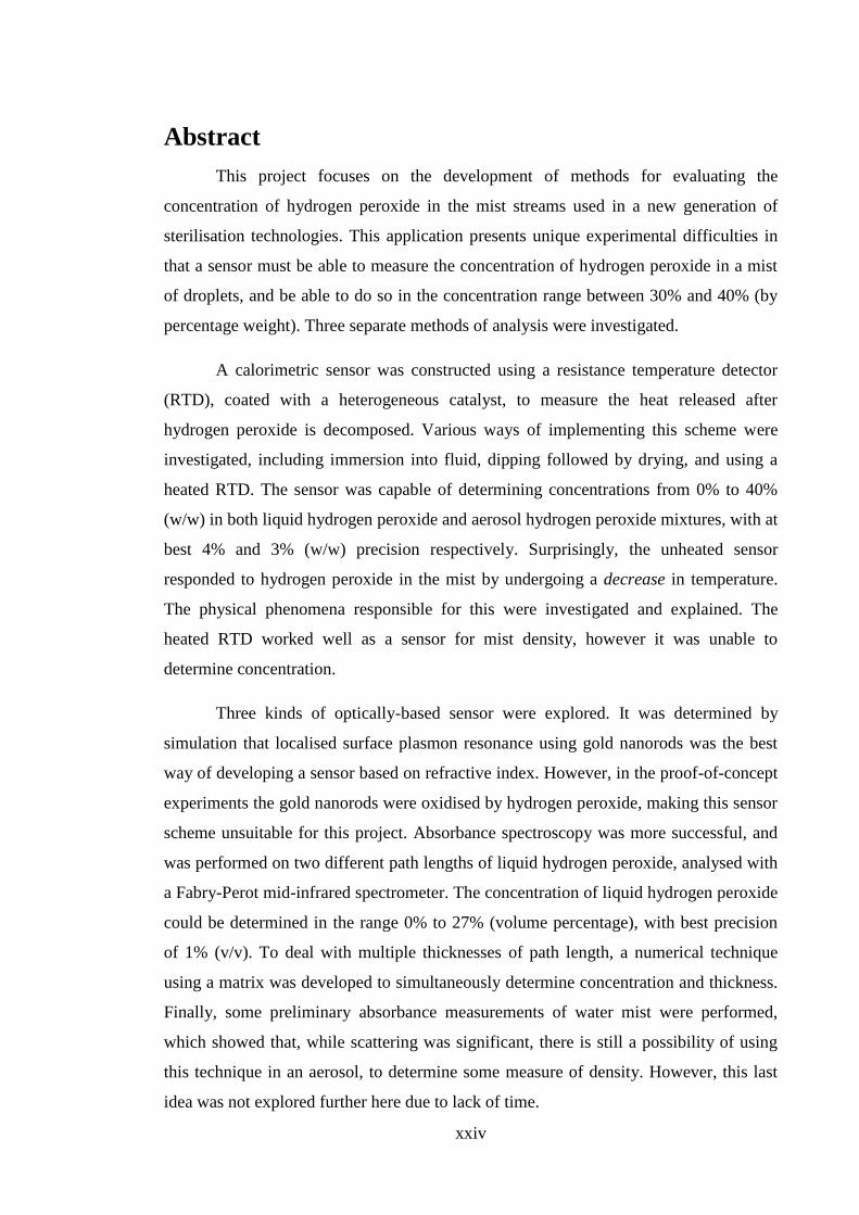
Abstract

This project focuses on the development of methods for evaluating the

concentration of hydrogen peroxide in the mist streams used in a new generation of

sterilisation technologies. This application presents unique experimental difficulties in

that a sensor must be able to measure the concentration of hydrogen peroxide in a mist

of droplets, and be able to do so in the concentration range between 30% and 40% (by

percentage weight). Three separate methods of analysis were investigated.

A calorimetric sensor was constructed using a resistance temperature detector

(RTD), coated with a heterogeneous catalyst, to measure the heat released after

hydrogen peroxide is decomposed. Various ways of implementing this scheme were

investigated, including immersion into fluid, dipping followed by drying, and using a

heated RTD. The sensor was capable of determining concentrations from 0% to 40%

(w/w) in both liquid hydrogen peroxide and aerosol hydrogen peroxide mixtures, with at

best 4% and 3% (w/w) precision respectively. Surprisingly, the unheated sensor

responded to hydrogen peroxide in the mist by undergoing a decrease in temperature.

The physical phenomena responsible for this were investigated and explained. The

heated RTD worked well as a sensor for mist density, however it was unable to

determine concentration.

Three kinds of optically-based sensor were explored. It was determined by

simulation that localised surface plasmon resonance using gold nanorods was the best

way of developing a sensor based on refractive index. However, in the proof-of-concept

experiments the gold nanorods were oxidised by hydrogen peroxide, making this sensor

scheme unsuitable for this project. Absorbance spectroscopy was more successful, and

was performed on two different path lengths of liquid hydrogen peroxide, analysed with

a Fabry-Perot mid-infrared spectrometer. The concentration of liquid hydrogen peroxide

could be determined in the range 0% to 27% (volume percentage), with best precision

of 1% (v/v). To deal with multiple thicknesses of path length, a numerical technique

using a matrix was developed to simultaneously determine concentration and thickness.

Finally, some preliminary absorbance measurements of water mist were performed,

which showed that, while scattering was significant, there is still a possibility of using

this technique in an aerosol, to determine some measure of density. However, this last

idea was not explored further here due to lack of time.

determination of hydrogen peroxide concentration in … · determination of hydrogen peroxide...

Documents