determinants of precautionary savings: elasticity of intertemporal substitution … · ·...

Determinants of Precautionary Savings: Elasticity of

Intertemporal Substitution vs. Risk Aversion

Arif Oduncu

Research and Monetary Policy Department

Central Bank of the Republic of Turkey

E-mail: [email protected]

Abstract

The purpose of this paper is to understand the effects of the elasticity of

intertemporal substitution (EIS), the percentage change in intertemporal consumption in

response to a given percentage change in the intertemporal price, and risk aversion on

savings separately and determine which coefficient is more important factor for

precautionary savings. This paper is an extension of Weil (1993)’ paper where the

determinants of precautionary savings can be studied analytically by assuming

exponential risk utility function in Epstein-Zin (1989) preferences. In my model, the

exponential risk utility function is not assumed in order to look at more general model.

Thus, the problem is not analytically solvable anymore. Instead, the problem is solved

numerically in order to determine which coefficient is more important factor for

precautionary savings. The result is saving increases as EIS increases. Similarly, saving

increases as the coefficient of risk aversion increases. More importantly, it is observed

that EIS is a more important factor for precautionary savings than risk aversion because

saving is more sensitive to changes in EIS than changes in risk aversion.

JEL classification: C61, C63, E21, E27

Keywords: Precautionary Savings, Epstein-Zin Utility, Risk Aversion, Household

Dynamic Decision Problem

1

1 Introduction

The main question that this paper tries to answer is whether the elasticity of

intertemporal substitution (EIS), the percentage change in intertemporal consumption in

response to a given percentage change in the intertemporal price, or risk aversion is more

important determinant of precautionary savings. This is an important question since a

significant fraction of the capital accumulation that occurs in the United States is due to

precautionary savings according to Zeldes (1989a), Skinner (1988) and Caballero (1990).

Thus, knowing the important determinant of precautionary savings will be helpful to

understand the capital accumulation mechanism in the U.S.

Zeldes (1989a) calculates the optimal amount of precautionary savings under

uncertain income environment for the agents who have constant relative risk aversion

utility. He finds that agents optimally choose to save more in an uncertain environment

than they would have done in a certain environment when there is no borrowing or

lending constraints. He uses numerical methods to closely approximate the optimal

saving. In Deaton (1991)’s paper, the agents are restricted in their ability to borrow to

finance consumption. However, nothing prevents these agents from saving and

accumulating assets in order to smooth their consumption in bad states. In this

environment, he shows that the behavior of saving and asset accumulation is quite

sensitive to what agents believe about the stochastic process generating their income.

Aiyagari (1994) modifies the standard growth model of Brock and Mirman (1972)

to include a role for uninsured idiosyncratic risk and borrowing constraints. In his model,

there are a large number of agents who receive idiosyncratic labor endowment shocks

that are uninsured. He analyzes its qualitative and quantitative implications for the

2

contribution of precautionary saving to aggregate saving, importance of asset trading, and

income and wealth distributions. He shows that aggregate saving is larger under

idiosyncratic risk than certainty. Therefore, he demonstrates that two household with

identical preferences over present and future consumption will under certainty save the

same, but this does not necessarily imply that these two households will save the same in

uncertain environments. In a recent work, Guvenen (2006) shows that aggregate

investment is mostly determined by wealthy people who have high EIS and aggregate

consumption is mostly determined by non-wealthy people who have low EIS. In his

model, there are two different types of agents who differ in elasticity of intertemporal

substitution and limited participation in the stock market. Limited participation is only

used to create substantial wealth inequality similar to the data. Thus, difference in the

elasticities is an important factor for determining savings.

My paper is an extension of Weil (1993)’ paper where the determinants of

precautionary savings can be studied analytically by assuming exponential risk utility

function in Epstein-Zin (1989) preferences. This assumption makes the problem

analytically solvable. Weil (1993) shows that savings increase in each of these cases:

• when persistence of income shocks increases

• when the coefficient of risk aversion increases

• when EIS increases

However, Weil does not rank the importance of these determinants in saving decisions.

The purpose of this paper is to understand the effects of the elasticity of

intertemporal substitution (EIS) and risk aversion on savings separately and determine

which coefficient is more important factor for precautionary savings. The numerical

3

calculations are performed for the more general form of the Epstein-Zin utility function

in order to calculate savings for different EIS and risk aversion, RA, coefficients to see

which one is the more important determinant of precautionary savings. In this paper, I

first look at the savings for different values of EIS by keeping the risk aversion

coefficient constant. Then, savings are calculated by changing the risk aversion

coefficients and keeping EIS constant. As a result, I obtained graph of savings for

different EIS and risk aversion coefficients.

According to Chatterjee, Giuliano and Turnovsky (2004), most of the existing

literature assumes that the preferences of the representative agent are represented by a

constant elasticity utility function. While this specification of preferences is convenient, it

is also restrictive in that two key parameters, the elasticity of intertemporal substitution

and the coefficient of relative risk aversion, become directly linked to one another and

cannot vary independently. This is a significant limitation and one that can lead to

seriously misleading impressions of the effects that each parameter plays in determining

the precautionary savings.

Arrow (1965) and Pratt (1964) introduced the concept of the coefficient of

relative risk aversion and it is well defined in the absence of any intertemporal

dimension. Hall (1978, 1988) and Mankiw, Rotemberg, and Summers (1985) established

the concept of the elasticity of intertemporal substitution and it is well defined in the

absence of risk. The standard constant elasticity utility function has the property that both

parameters EIS and RA are constant, though it imposes the restriction EIS*RA = 1 with

the widely employed logarithmic utility function corresponding to EIS=RA=1. Thus it is

important to realize that in imposing this constraint the constant elasticity utility function

4

is also invoking these separability assumptions according to Giuliano and Turnovsky

(2003).

Although there are empirical studies about the value of the elasticity of

intertemporal substitution, the results are different from each other. Hall (1988) and

Campbell and Mankiw (1989) estimate EIS 0.1 based on macro data. Epstein and Zin

(1991) provide estimates spanning the range 0.05 to 1, with clusters around 0.25 and 0.7.

Attanasio and Weber (1993, 1995) find that their estimate of EIS is 0.3 using aggregate

data and is 0.8 using cohort data. They propose that the aggregation implicit in the macro

data may cause a significant downward bias in the estimate of EIS. Beaudry and van

Wincoop (1995) estimate EIS near 1. More recent estimates by Ogaki and Reinhart

(1999) suggest values of around 0.4. Moreover, Atkeson and Ogaki (1996) and Ogaki and

Atkeson (1997) find evidence to suggest that the EIS increases with household wealth. As

a result of these findings, the variation of EIS from 0.04 to 0.99 is used in the numerical

calculations.

Similar to the elasticity of intertemporal substitution, the value the coefficient of

risk aversion shows a discrepancy in the literature. Epstein and Zin (1991) conclude that

their estimate of RA is near 1. In contrast, Kandel and Stambaugh (1991) take RA as 30

and Obstfeld (1994a) takes RA as 18. More recent study by Constantinides, Donaldson,

and Mehra (2002) present that empirical evidence suggests that RA is most plausibly

around 5. According to these findings, the variation of RA from 1.01 to 25 is used in the

numerical calculations.

Zeldes (1989a), Deaton (1991) and Aiyagari (1994) use expected value of a

discounted sum of time-additive utilities in the model, thus the motion of risk aversion

5

and EIS is confused. As a result, it is not possible to look at the effects of EIS and risk

aversion separately. According to Giuliano and Turnovsky (2003), this is important for

two reasons. First, conceptually, EIS and RA impinge on the economy in quite

independent, and in often conflicting ways. They therefore need to be decoupled if the

true effects of each are to be determined. Risk aversion impinges on the equilibrium

through the portfolio allocation process, and thus through the equilibrium risk that the

economy is willing to sustain. It also determines the discounting of risk in deriving the

certainty equivalent level of income. The intertemporal elasticity of substitution then

determines the allocation of this certainty equivalent income between current

consumption and future consumption. Second, the biases introduced by imposing the

compatibility condition EIS*RA=1 for the constant elasticity utility function can be quite

large, even for relatively weak violations of this relationship. According to Chatterjee,

Giuliano and Turnovsky (2004), while one certainly cannot rule out using the constant

elasticity utility function, as a practical matter, their results suggest that it should be

employed with caution, recognizing that if the condition for its valid use is not met, very

different implications may be drawn.

This paper follows Weil (1993) by using an Epstein-Zin utility function that

permits risk attitudes to be disentangled from the degree of intertemporal substitutability.

This facilitates the study of the effects of EIS and risk aversion separately. It is shown

saving increases as EIS increases. Similarly, saving increases as the coefficient of risk

aversion increases. More importantly, it is observed that EIS is a more important factor

for precautionary savings than risk aversion because saving is more responsive to

changes in EIS than changes in risk aversion. For example, starting from the benchmark

6

preference parameters RA= 5 and EIS = 0.2, the constant elasticity utility function

implies that doubling RA to 10 (and thus simultaneously halving EIS to 0.1 so that

EIS*RA=1) would reduce the savings to 0.9148 when the savings in benchmark case is

normalized to 1. On the other hand, when the EIS is doubled to 0.4 and RA is halved to

2.5, the savings increases to 1.4074. In the unrestricted utility function, if RA increases

two times, RA=10, and EIS stays the same, the savings become 1.3838 whereas if EIS

increases twice, EIS=0.4, and RA stays the same, the savings become 1.9083. Thus, the

change in savings is much less sensitive to the degree of risk aversion than to the

intertemporal elasticity of substitution.

The paper is structured as follows. Section 2 describes the model, by explaining

the preferences and the optimization problem faced by individuals in the economy. The

numerical results are presented and discussed in Section 3. Section 4 concludes the paper

by outlining some directions for future research. The appendix describes the numerical

solution of the model.

2 Model

Our model is the standard problem of a representative agent who lives for many

periods and chooses optimal current consumption and next period’s bond holding in order

to maximize the utility function. The source of uncertainty considered is in exogenous

future income and there exist no markets in which agents can insure against this

uncertainty. Although agents can save by holding bonds, they are not able to borrow, i.e.

there is a borrowing constraint.

7

Preferences

Following Weil’s (1993) terminology, a representative agent whose preferences

over deterministic consumption stream exhibit a constant elasticity of intertemporal

substitution:

W(c�, c��, c��, … ) = �(1 − �) ∑ ��

�� (1)

where 1

(1 )ρ

ϕ=

−> 0 is the elasticity of intertemporal substitution, EIS, and β ϵ (0,1) is

the constant exogenous discount factor. These preferences can be represented recursively

as:

W(c�, c��, c��, … ) = �[c�, W(c��, c��, c��, … )] (2)

= �(1 − �)�� + � {W(c��, c��, c��, … )}��

�� (3)

where U(.,.) is an aggregator function. Behavior towards risk is summarized by a constant

coefficient of risk aversion, denoted by the parameter α >1.

#$ = (%#′�'∝)�

�)* (4)

Equation 4 defines the utility certainty equivalent of a lottery yielding a random

utility level #+ is #$ for the representative agent where E is expectation operator.

W$ (c��, , c��, , c��, , … ) represents the certainty equivalent, conditional on time t

information, of time t+1 utility. It is assumed that preferences over random consumption

lotteries have the recursive representation with the aggregator function. Therefore,

current utility becomes the aggregate of current consumption and the certainty equivalent

of future utility as seen in Equation 5.

W(c�, c��, , c��, , … ) = �[c�, W$ (c��, , c��, , c��, , … )] (5)

8

This utility function has both a constant elasticity of intertemporal substitution,

1

(1 )ρ

ϕ=

−, and a constant coefficient of risk aversion, α. This utility function

distinguishes EIS and RA explicitly. This facilitates the study of the effects of EIS and

risk aversion separately.

Utility Function

This utility function is used to calculate the determinants of precautionary

savings:

11 1

1[ (1 ) ( ) ( ( ) ) ]t t t tU C E Uϕ

ϕ ϕα αβ β − −+= − +

where β is time discount factor, Ct is consumption today, 1

(1 )ρ

ϕ=

− is the EIS and α is

the coefficient of risk aversion. This type of utility preference allows us to disentangle the

EIS and the risk aversion and examine their effects independently. Also, being third

derivative of utility function is positive, �+++ > 0, introduces prudence into the decisions

of the consumer.

Weil (1993) assumes the exponential risk utility function in Epstein-Zin (1989)

preferences and so the determinants of precautionary savings can be studied analytically.

In other words, this assumption makes the problem analytically solvable.

However, in my model, the exponential risk utility function is not assumed in

order to look at more general model. Thus, the problem is not analytically solvable

anymore. Instead, the problem is solved numerically for the model that is more general

than the model of Weil (1993).

9

Budget Set

When y denotes today’s income, b denotes today’s bond holding, C denotes

today’s consumption, -+ tomorrow’s bond holding and R denotes the interest rate, the

budget constraint of the representative agent for each period becomes as seen in Equation

6 below.

. + -+ ≤ 0- + 1 (6)

Household Dynamic Decision Problem

The agent solves her problem recursively in a given state. The optimal solution to

this problem is characterized most simply in terms of a value function, V(y,b). The agent

knows today’s income, y, and bond holding, b, and chooses today’s consumption, c, and

tomorrow’s bond holding, -+, in order to maximize the utility function as a dynamic

programming problem:

1

1

, '

( , ) [ (1 )( ) ( ( ( ', ') | ) ]m a xC b

V y b C E V y b yϕ

ϕ ϕαβ β −= − +

s.t

. + -+ ≤ 0- + 1 (7)

1+= ( )yΓ (8)

-+ ≥ 0 (9)

C ≥ 0 (10)

where E denotes the mathematical expectation operator conditional on information

available today. As said earlier, Equation 7 is the budget constraint. Equation 8 is the law

of motion for income and it is a Markov Process getting two different income values,

10

income low and income high, in the numerical calculations. Equation 9 shows the

borrowing constraint and shows that asset holding or saving cannot be negative. Equation

10 shows that consumption cannot be negative. The time discount factor, β is chosen

smaller than 1/R in order to prevent agents to save infinitely which is proved in Aiyagari

(1994) that if β is larger than 1/R, agents save infinitely. Furthermore, the coefficient of

risk aversion, α , is greater than 1 and the coefficient of EIS,1

(1 )ρ

ϕ=

− , is between

0.04 and 0.99.

3 Results

In the model, the law of motion for income is a Markov Process in which agents

can get only two different amounts of exogenous income, income low and income high.

There is an assignment of the probability of getting the same income that defines the

persistence of income shocks. As discussed in the introduction section, the EIS varies

from 0.04 to 0.99 and the risk aversion (RA) varies from 1.01 to 25 as according to the

estimates of these coefficients in the literature.

The model is simulated for 1000 periods in order to make the bond holdings

converge to a stochastic steady state. Then, the agent’s savings are summed from period

300 to 1000 and divided by 701. As a result, the findings are the average savings of the

agent. The numerical solution of the model is explained explicitly in the Appendix.

For the time discount factor, β = 0.955 and the probability of getting the same

income, persistence of income shocks, is 0.7, the savings are shown in Table 1 below:

11

Table 1: Savings when persistence is 0.7

Probability=0.7 EIS

0.05 0.1 0.2 0.4 0.8 0.99

Risk Aversion

20

0.8795 1.1607 1.6916 2.7664 5.8416 9.7270

10

0.4863 0.9148 1.3838 2.3787 5.2578 9.0545

5

0.4057 0.8258 1.0000 1.9083 4.6570 8.2933

2.5

0.2903 0.4699 0.6960 1.4074 4.0172 7.4701

1.25

0.2279 0.3220 0.5079 1.0249 3.3490 6.5828

1.01

0.2010 0.2839 0.4476 0.8789 3.0111 6.2032

The benchmark preference parameters are RA= 5, EIS = 0.2 and the probability of

getting the same income is 0.7. The savings in benchmark case is normalized to 1 and the

savings for various parameters are proportions to the savings of benchmark case. For

instance, if RA is doubled to 10 by implying the constant elasticity utility function (thus

simultaneously halving EIS to 0.1 so that EIS*RA=1), the savings reduces to 0.9148. On

the other hand, when the EIS is doubled to 0.4 and RA is halved to 2.5, the savings

increases to 1.4074. In the unrestricted utility function, if RA increases two times,

RA=10, and EIS stays the same, the savings become 1.3838 whereas if EIS increases

twice, EIS=0.4, and RA stays the same, the savings become 1.9083. Thus, the change in

savings is much less sensitive to the degree of risk aversion than to the intertemporal

elasticity of substitution.

12

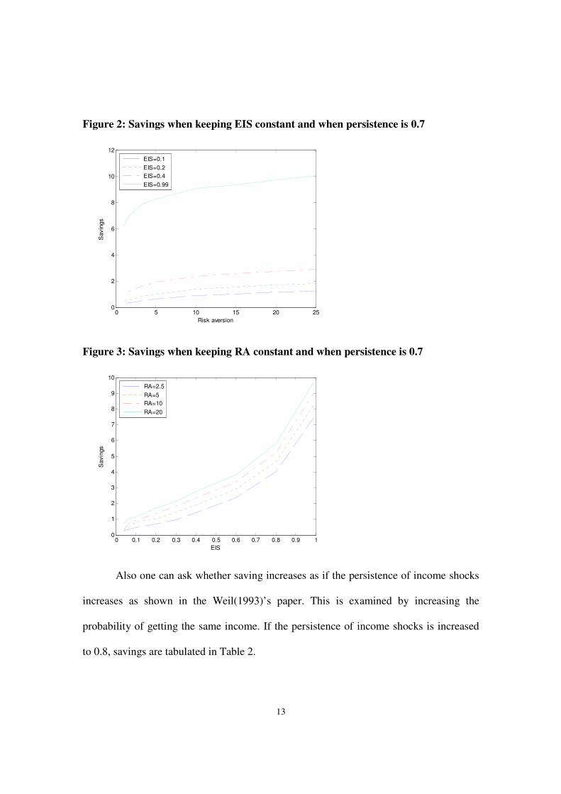
The three dimensional graph of savings according to different parameters of the

elasticity of intertemporal substitution and risk averse is depicted in Figure 1. The figure

demonstrates that, as similar to the results in the Weil(1993)’s paper , saving increases

when the parameter of EIS increases by keeping risk aversion constant because an

increase in the elasticity of intertemporal substitution increases the propensity to consume

out of wealth and out of current income. Also, saving increases when the parameter of

risk aversion increases by keeping EIS constant as expected since the more risk averse

the agent is, the stronger his precautionary saving motive. More prominently, I observe

that EIS is more important in precautionary saving decision than risk aversion since

saving is more responsive to changes in EIS than changes in risk aversion as portrayed in

Figure 2 and Figure 3.

Figure 1: 3-D graph of savings when persistence is 0.7

00.2

0.40.6

0.81

0

10

20

300

2

4

6

8

10

12

EISRisk Aversion

Savin

gs

13

Figure 2: Savings when keeping EIS constant and when persistence is 0.7

Figure 3: Savings when keeping RA constant and when persistence is 0.7

Also one can ask whether saving increases as if the persistence of income shocks

increases as shown in the Weil(1993)’s paper. This is examined by increasing the

probability of getting the same income. If the persistence of income shocks is increased

to 0.8, savings are tabulated in Table 2.

0 5 10 15 20 250

2

4

6

8

10

12

Risk aversion

Savin

gs

EIS=0.1

EIS=0.2

EIS=0.4

EIS=0.99

0 0.1 0.2 0.3 0.4 0.5 0.6 0.7 0.8 0.9 10

1

2

3

4

5

6

7

8

9

10

EIS

Savin

gs

RA=2.5

RA=5

RA=10

RA=20

14

Table 2: Savings when persistence is 0.8

Probability=0.7 EIS

0.05 0.1 0.2 0.4 0.8 0.99

Risk Aversion

20

1.1238 1.5943 2.3077 3.6695 7.6213 12.5308

10

0.6277 1.1794 1.8532 3.0868 6.7874 11.6185

5

0.5128 0.8944 1.2281 2.3364 5.7818 10.4551

2.5

0.3268 0.5706 0.7397 1.5477 5.8636 9.0654

1.25

0.2195 0.3768 0.5013 1.0132 3.5628 7.4995

1.01

0.1911 0.2767 0.4350 0.8577 3.0529 6.7754

For the parameters RA=5 and EIS=0.2, the savings is 1.2281. It means there is

about 22.8 % increase if the persistence increases from 0.7 to 0.8 since the savings in the

benchmark case is normalized to 1 and in the benchmark case preference parameters are

RA= 5, EIS = 0.2 and the probability of getting the same income is 0.7. In the constant

elasticity utility function, if RA is multiplied by 4 and RA becomes 20 (thus

simultaneously halving EIS to 0.05 so that EIS*RA=1), the savings reduces to 1.1238

from 1.2281. The percentage reduction is 8.5 %. On the other hand, when the EIS is

multiplied by 4 to make EIS=0.8 and RA becomes to 1.25, the savings increases to

3.5628 and the percentage raise is 190.1 %. In the unrestricted utility function, if RA

increases four times, RA=20, and EIS stays the same, the savings become 2.3077

whereas if EIS increases four times, EIS=0.8, and RA stays the same, the savings become

15

5.7818. As seen from percentages, it is clear that saving is much more responsive to

changes in EIS than to changes in risk aversion.

The persistence of income shocks is a determinant of the strength of precautionary

savings motive. The more persistent the income process, the more responsive current

consumption to fluctuations in current income. Therefore, the more persistence in income

shocks leads to a stronger precautionary savings motive as seen in Table 2.

The three dimensional graph of savings according to different parameters of the

elasticity of intertemporal substitution and risk aversion when the persistence of income

shocks is 0.8 is depicted in Figure 4 below. Also, the savings when keeping EIS constant

and when keeping RA constant portrayed in Figure 5 and Figure 6 respectively.

Figure 3: 3-D graph of savings when persistence is 0.8

0 0.2 0.4 0.60.8 1

0

1020

300

2

4

6

8

10

12

14

EISRisk Aversion

Savin

gs

16



It is explained that savings increase when persistence of income shocks increases

in Weil(1993)’s paper. It is shown in the figures below that the savings when probability

is 0.8 is larger than the savings when probability is 0.7. It is also observed the same result

that EIS is a more significant determinant of savings than risk aversion for each

probability.

0 5 10 15 20 250

2

4

6

8

10

12

14

Risk aversion

Savin

gs

EIS=0.1

EIS=0.2

EIS=0.4

EIS=0.99

0 0.1 0.2 0.3 0.4 0.5 0.6 0.7 0.8 0.9 10

2

4

6

8

10

12

14

EIS

Savin

gs

RA=2.5

RA=5

RA=10

RA=20

17

Figure 7: Savings when EIS=0.2 for persistence 0.7 and 0.8

Figure 8: Savings when Risk Aversion=5 for persistence 0.7 and 0.8

The savings are calculated also when persistence of income shock is 0.5. When

the persistence is 0.5, the savings for the benchmark parameters, EIS=5 and RA=1, is

0.55 and so there is 45 % decrease if the persistence decreases from 0.7 to 0.5. In the

constant elasticity utility function, if RA is multiplied by 5 and RA becomes 25 (thus

simultaneously halving EIS to 0.04 so that EIS*RA=1), the savings reduces to 0.41 from

0.55 and so the percentage reduction becomes 25 %. On the other hand, when the EIS is

0 5 10 15 20 250

0.5

1

1.5

2

2.5

Risk Aversion

Savin

gs

Prob=0.7

Prob=0.8

0 0.1 0.2 0.3 0.4 0.5 0.6 0.7 0.8 0.9 10

2

4

6

8

10

12

EIS

Savin

gs

Prob=0.7

Prob=0.8

18

multiplied by 5 to make EIS=0.99 and RA becomes to 1.01, the savings increases to 4.26

and the percentage raise is 675 %. The similar results are obtained that EIS is more

important determinant of precautionary savings as shown in the figures below.



0 5 10 15 20 250

1

2

3

4

5

6

Risk aversion

Savin

gs

EIS=0.1

EIS=0.2

EIS=0.4

EIS=0.99

0 0.1 0.2 0.3 0.4 0.5 0.6 0.7 0.8 0.9 10

1

2

3

4

5

6

EIS

Savin

gs

RA=2.5

RA=5

RA=10

RA=20

19

If the persistence decreases from 0.7 to 0.6, there is 31 % decrease in the savings

for the benchmark parameters since the savings 0.69 in this case. In the constant elasticity

utility function, if EIS is multiplied by 2 and EIS becomes 0.4 (thus simultaneously

halving RA to 2.5 so that EIS*RA=1), the savings rise to 1.02 from 0.69 and so the

percentage raise becomes 48 %. On the other hand, when the RA is multiplied by 2 to

make RA= 10 and EIS becomes to 0.1, the savings shrinks to 0.62 and the percentage

reduction is 10 %. In the unrestricted utility function, if EIS increases two times,

EIS=0.4, and RA stays the same, the savings become 1.35 whereas if RA increases two

times, RA=10, and EIS stays the same, the savings become 0.95. The increase is 96 % in

the first case and 38 % in the second case. As seen from percentages, it is clear that

saving is much more responsive to changes in EIS than to changes in risk aversion. The

results are as portrayed in the Figure 11 and Figure 12 below.


0 5 10 15 20 250

1

2

3

4

5

6

7

8

Risk aversion

Savin

gs

EIS=0.1

EIS=0.2

EIS=0.4

EIS=0.99

20


As mentioned earlier, the persistence of income shocks is a determinant of the

strength of precautionary savings motive. The more persistence in income shocks leads to

a stronger precautionary savings. It is shown in the Figure 13 and Figure 14 below that

the savings when the persistence of income shocks is 0.6 is larger than the savings when

persistence is 0.5. The ratio of the savings when persistence is 0.5 to the savings when

persistence is 0.6 ranges from 0.70 to 0.89 by comparing the savings with the same

parameter values for the coefficients of elasticity of intertemporal substitution and risk

aversion. The range is wider when keeping the EIS=0.2 constant and changing the

coefficient of risk aversion than when keeping the RA=5 constant and changing the

coefficient of elasticity of intertemporal substitution as seen in Figure 13 and Figure 14

below.

Moreover, it is also observed the same result that EIS is a more crucial

determinant of savings than risk aversion for each persistence of income shocks since

saving is more sensitive to changes in EIS than in risk aversion.

0 0.1 0.2 0.3 0.4 0.5 0.6 0.7 0.8 0.9 10

1

2

3

4

5

6

7

8

EIS

Savin

gs

RA=2.5

RA=5

RA=10

RA=20

21

Figure 13: Savings when EIS=0.2 for persistence 0.5 and 0.6

Figure 14: Savings when Risk Aversion=5 for persistence 0.5 and 0.6

0 5 10 15 20 250.2

0.4

0.6

0.8

1

1.2

1.4

1.6

Risk Aversion

Savin

gs

Prob=0.5

Prob=0.6

0 0.1 0.2 0.3 0.4 0.5 0.6 0.7 0.8 0.9 10

1

2

3

4

5

6

7

EIS

Savin

gs

Prob=0.5

Prob=0.6

22

4 Conclusion and Discussion

In this paper, I attempt to determine the important factors of precautionary saving.

Saving under temporal risk aversion and intertemporal substitution usually exceeds the

certainty-equivalent level of saving and this type of prudent behavior is called the

precautionary motive for saving. Precautionary saving arises when consumers are risk

averse and have elastic intertemporal preferences and so hedge against unanticipated

future declines in income. The precautionary motive induces individuals to save in order

to provide insurance against future periods in which their incomes are low or their needs

are high according to Van der Ploeg (1993). I look at the effects of EIS and risk aversion

to savings separately by using Epstein-Zin (1989) recursive utility function. I use

Epstein-Zin (1989) utility since this utility permit risk attitudes to be disentangled from

the degree of intertemporal substitutability and provides a motive for precautionary

saving.

According to Chatterjee, Giuliano and Turnovsky (2004), most of the existing

literature assumes that the preferences of the representative agent are represented by a

constant elasticity utility function. While this specification of preferences is convenient, it

is also restrictive in that two key parameters, the elasticity of intertemporal substitution

and the coefficient of risk aversion, become directly linked to one another and cannot

vary independently. This is a significant limitation and one that can lead to seriously

misleading impressions of the effects that each parameter plays in determining the

precautionary savings. With the diversity of empirical evidence suggesting that this

constraint, EIS*RA=1, may or may not be met, it is important that studies of these two

parameters impinges on the equilibrium in very distinct and in some respects conflicting

23

ways. Therefore, the general conclusion to be drawn is that errors committed by using the

constant elasticity utility function, even for small violations of the compatibility condition

within the empirically plausible range of the parameter values, can be quite substantial.

While one certainly cannot rule out using the constant elasticity utility function, as a

practical matter, their results suggest that it should be employed with caution, recognizing

that if the condition for its valid use is not met, very different implications may be drawn.

Hall (1988) points out that intertemporal substitution by consumers is a central

element of most modern macroeconomic models. Weil (1993) shows that when the

coefficient of elasticity of intertemporal substitution increases savings increase. Atkeson

and Ogaki (1996) develop and estimate a model of preferences which formalizes the

intuition that poor consumers have a lower intertemporal elasticity of substitution than do

rich consumers because expenditure inelastic goods (necessary goods) are less

substitutable over time than are expenditure-elastic goods. Guvenen (2006) shows that

aggregate saving is mostly determined by wealthy people who have high EIS and

aggregate consumption is mostly determined by non-wealthy people who have low EIS.

Weil (1993) and Van der Ploeg (1993) show that when the coefficient of risk aversion

increases savings increase. The saving increases as EIS increases and as the coefficient of

risk aversion increases is observed in this paper. More importantly, it is examined that

EIS is a more important factor for precautionary savings than risk aversion because

saving is more responsive to changes in EIS than changes in risk aversion. This finding

sheds new light on precautionary savings. Knowing that EIS is more significant

contributor to the precautionary savings is important since a significant fraction of the

24

capital accumulation that occurs in the United States is due to precautionary savings

according to Zeldes (1989a).

The main limitation of the model of precautionary savings I have introduced in

this paper is in future income process. The Markov process is used in the paper where the

future income takes only two different values, high income and low income, for

simplicity. Investigating other income processes would be a good improvement and

future research for giving more representation of the precautionary savings motive. Yet,

this model sheds new light on the determinant of precautionary savings in multi-period

economics and determines the coefficient of elasticity of intertemporal substitution is a

more important factor for precautionary savings than the coefficient of risk aversion

because saving is more responsive to changes in the coefficient of elasticity of

intertemporal substitution than changes in the coefficient of risk aversion.

25

Appendix: Numerical Solution

This section describes the numerical solution of the model. The state values of the

agent are today’s income and bond holding. Then, agent chooses the today’s consumption

and tomorrow’s bond holding, none of them can be negative. Tomorrow’s income is

determined as a law of motion.

Step1: Initialization

• The interest rate, discount factor, coefficient vectors of EIS and risk aversion are

determined. There are two different income values, income low and income high,

and different probabilities ranging from 0.5 to 0.8 for the Markov process of

income so uncertainty in income in the model comes from this process. EIS

changes from 0.04 to 0.99 and Risk aversion changes from 1.01 to 25.The interest

rate can be two different values, either 1.03 or 1.04. Thus, calculations are

performed for these each different values of income, EIS, risk aversion, interest

rate and probabilities.

• There are 100 grid points for the initial bond holdings. I execute value function

iteration and determine tomorrow’s bond holding for each case by initially

assuming -+=b. I am able to use the linear interpolation to evaluate tomorrow’s

bond holding and the value function for off the grid points since the value

function is linear in individual wealth in Epstein-Zin preferences .

Step 2: Household Dynamic Decision Problem

• I start with a household who has an initial income and zero bond at first period

and the household decides for current consumption and bond holding of second

26

period. I iterate the process unless the bond holding process converges to a

stochastic steady state. I observe 1000 iterations are adequate for the convergence.

• For the income process, I generate pseudo random process for each probabilities

of the Markov Process by using “randsrc” function in MATLAB. I generate two

different pseudo random processes for two different income values according to

probabilities and then produce the real income process that the agent faces in the

iteration from those random processes.

27

References

Aiyagari, R., 1994. Uninsured idiosyncratic shock and aggregate saving, Quarterly

Journal of Economics, 109, 659-84.

Arrow, K., 1965. Aspects of the theory of risk-bearing. Yrjö Jahnsson Foundation,

Helsinki.

Atkeson, A. and Ogaki, M., 1995. Wealth-varying intertemporal elasticities of

substitution: evidence from panel and aggregate data. Journal of Monetary Economics,

38, 507-34.

Attanasio, O. and Weber, G., 1993. Consumption growth, the interest rate, and

aggregation. Review of Economic Studies, 60, 631-49.

Attanasio, O. and Weber, G., 1995. Is consumption growth consistent with intertemporal

optimization? Evidence from the consumer expenditure survey. Journal of Political

Economy, 103, 1121-57.

Beaudry, P. and van Wincoop, E., 1995. The intertemporal elasticity of substitution: an

exploration using US panel of state data. Economica, 63, 495-512.

Brock, W. and Mirman, L., 1972. Optimal economic growth and uncertainty: The

discounted case. Journal of Economic Theory, 4, 479-513.

Caballero, R., 1990. Consumption puzzles and precautionary savings. Journal of

Monetary Economics, 25, 113-36.

Campbell, J. and Mankiw, N., 1989. Consumption, income, and interest rates:

reinterpreting the time series evidence. In: Blanchard, O., Fischer,S., (Eds.), NBER

Macroeconomic Annual, MIT Cambridge MA, 185-216.

Chatterjee, S., Giuliano, P. and Turnovsky, S., 2004. Capital Income Taxes and Growth

in a Stochastic Economy: A Numerical Analysis of the Role of Risk Aversion and

Intertemporal Substitution. Journal of Public Economic Theory, 6, 277-310.

Chou, R., Engle R. and Kane A., 1992. Measuring risk aversion on excess returns on a

stock index. Journal of Econometrics, 52, 210-24.

Constantinides, G.M., Donaldson, J.B. and Mehra, R., 2002. Junior can't borrow: a new

perspective on the equity premium puzzle. Quarterly Journal of Economics, 117, 269-96.

Deaton, A., 1991. Saving and liquidity constraints. Econometrica, 59, 1221-48.

28

Giuliano, P. and Turnovsky, S., 2003. Intertemporal Substitution, Risk Aversion, and

Economic Performance in a Stochastically Growing Open Economy. Journal of

International Money and Finance, 22, 529-56.

Guvenen, F., 2006. Reconciling conflicting evidence on the elasticity of

intertemporal substitution: A Macroeconomic perspective. Journal of Monetary

Economics, 53, 1451-72.

Eichenbaum, M. and Hansen, L., 1990. Estimating models with intertemporal substitution

Using aggregate time series data. Journal of Business, Economics and Statistics, 8, 53–

69.

Epstein, L. and Zin, S., 1989. Substitution, risk aversion, and the temporal behavior of

consumption and asset returns: A theoretical framework. Econometrica, 57, 937-69.

Epstein, L., and Zin S., 1991. Substitution, risk aversion, and the temporal behavior of

consumption and asset returns: An empirical analysis. Journal of Political Economy, 99,

263-86.

Fauvel, Y. and Samson, L., 1991. Intertemporal substitution and durable goods: An

empirical analysis. Canadian Journal of Economics, 24, 192–205.

Hall, R., 1978. Stochastic implications of the life-cycle permanent income hypothesis:

theory and evidence. Journal of Political Economy, 86, 971-87.

Hall, R., 1988. Intertemporal substitution in consumption. Journal of Political Economy,

96, 339-57.

Kandel, S. and Stambaugh, R., 1991. Asset returns and intertemporal preferences.

Journal of Monetary Economics, 27, 39-71.

Kreps, D. and Porteus, E., 1978. Temporal resolution of uncertainty and dynamic choice

theory. Econometrica, 96, 185-200.

Kreps, D. and Porteus, E., 1979. Dymanic choice theory and dynamic programming.

Econometrica, 97, 91-100.

Mankiw, N., Rotemberg, J. and Summers, L., 1985. Intertemporal substitution in

macroeconomics. Quarterly Journal of Economics, 100, 225-51.

McLaughlin, K., 1995. Intertemporal substitution and λ−constant comparative statics.


Meghir, C. and Weber, G., 1991. Intertemporal non-separability or borrowing

eestrictions? Manuscript. London: Inst. Fiscal Studies.

29

Obstfeld, M., 1994a. Risk-taking, global diversification, and growth. American Economic

Review, 84, 1310-29.

Obstfeld, M., 1994b. Evaluating risky consumption paths: the role of intertemporal

substitutability. European Economic Review, 38, 1471-86.

Ogaki, M. and Atkeson, A., 1997. Rate of time preference, intertemporal substitution, and

the level of wealth. Review of Economics and Statistics, 79, 564-72.

Ogaki, M. and Reinhart, C.M., 1998. Measuring intertemporal substitution: the role of

durable goods. Journal of Political Economy, 106, 1078-98.

Ogaki, M. and Zhang, Q., 2001. Decreasing relative risk aversion and tests of risk

sharing. Econometrica, 69, 515-26.

Pratt, J., 1964. Risk aversion in the small and in the large. Econometrica, 32, 122-36.

Runkle, D., 1991. Liquidity constraints and the permanent-income hypothesis: evidence

from panel data. Journal of Monetary Economics, 27, 73-98.

Skinner, J., 1988. Risky income life cycle consumption and precautionary savings.


Van der Ploeg, F., 1993. A closed-form solution for a model of precautionary saving.

Review of Economic Studies, 60, 385-95.

Vissing-Jørgensen, A. 2002. Limited asset market participation and the elasticity of

intertemporal substitution. Journal of Political Economy, 110, 825-853.

Weil, P. 1990. Non-expected utility in Macroeconomics. Quarterly Journal of

Economics, 24, 401-21.

Weil, P. 1993. Precautionary savings and the permanent income hypothesis. Review of

Economic Studies, 60, 367-83.

Zeldes, S.,1989a. Optimal consumption with stochastic income: Deviations from

equivalence. Quarterly Journal of Economics, 104, 275-98.

determinants of precautionary savings: elasticity of intertemporal substitution … · ·...

Documents